new approaches for urban and regional air pollution ...cdn.intechweb.org/pdfs/17393.pdf · new...

22

New Approaches for Urban and Regional Air Pollution Modelling and Management

Salvador Enrique Puliafito, David Allende, Rafael Fernández, Fernando Castro and Pablo Cremades

Grupo de Estudios Atmosféricos y Ambientales (GEAA) Universidad Tecnológica Nacional – Facultad Regional Mendoza

Consejo Nacional de Investigaciones Científicas y Técnicas (CONICET) Argentina

1. Introduction

Air pollution is a complex problem that plays a key role in human well-being, environment

and climate change. Since cities are, by nature, concentrations of humans, materials and

activities, air pollution is clearly a typical phenomenon associated with urban centres and

industrialized regions (Fenger, 1999; de Leeuw et al., 2001). Since approximately half the

population of the world lives in medium to large cities, it is essential to evaluate the air quality

levels of the atmosphere in order to assess the possible health impact from exposition to

pollutants (World Health Organization [WHO], 2002; Brunekreef & Holgate, 2002).

Additionally, air pollution is not only a human health problem: the effects of pollution in

ecosystems and materials are well identified and documented (Fowler et al., 2009); economic

costs can also be associated with poor air quality, and with political/governmental measures

taken in order to prevent or reduce pollution (Muller & Mendelsohn (2007)).

The simplest technique for evaluating patterns of local-scale urban air pollution

concentration involves the interpolation of ambient concentrations from existing monitoring

networks (Ballesta et al., 2008; Ferretti et al., 2008). However, the measured data from these

stations are not necessarily representative of areas beyond their immediate vicinity, since

concentrations of pollutants in urban areas may greatly vary on spatial scales that range

from tens to hundreds of metres. At the same time, the temporal behaviour of primary and

secondary pollutants changes considerably between day and night due to solar radiation, so

that daily average measurements become unsatisfactory in determining or explaining high

pollution episodes.

Air Quality Models (AQMs) are mathematical tools that simulate the physical and chemical processes that involve air pollutant dispersion and reaction in the atmosphere. Furthermore, they improve the limitations of monitoring networks by providing prediction of the temporal and spatial distribution of actual pollution levels. Modelling studies, in combination with air quality monitoring, are then essential and complementary tools for long and short term air pollution control strategies. A well calibrated model is a unique tool that allows the representation of the atmospheric dynamics and chemistry. Thus, AQMs have become a valid instrument for environmental managers in many activities, such as

www.intechopen.com

Advanced Air Pollution

430

a) setting emission control regulations, b) testing the compliance of actual pollution levels, c) predicting the impact of new facilities on human health, d) selecting the best location for monitoring stations, and e) assessing the impact of different emissions scenarios on Global Climate Change. This Chapter presents an overview of several techniques and available codes applied to urban modelling, plus describing three study cases from different approaches that we have selected according to the magnitude of the simulated problem.

2. Air Quality Models (AQMs)

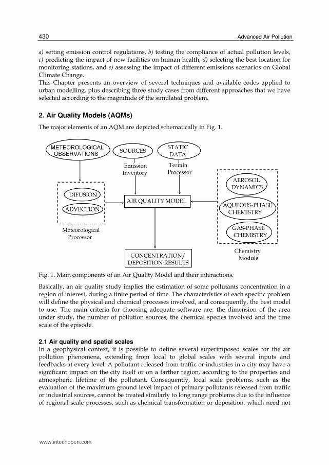
The major elements of an AQM are depicted schematically in Fig. 1.

Fig. 1. Main components of an Air Quality Model and their interactions.

Basically, an air quality study implies the estimation of some pollutants concentration in a region of interest, during a finite period of time. The characteristics of each specific problem will define the physical and chemical processes involved, and consequently, the best model to use. The main criteria for choosing adequate software are: the dimension of the area under study, the number of pollution sources, the chemical species involved and the time scale of the episode.

2.1 Air quality and spatial scales In a geophysical context, it is possible to define several superimposed scales for the air pollution phenomena, extending from local to global scales with several inputs and feedbacks at every level. A pollutant released from traffic or industries in a city may have a significant impact on the city itself or on a farther region, according to the properties and atmospheric lifetime of the pollutant. Consequently, local scale problems, such as the evaluation of the maximum ground level impact of primary pollutants released from traffic or industrial sources, cannot be treated similarly to long range problems due to the influence of regional scale processes, such as chemical transformation or deposition, which need not

www.intechopen.com


431

to be taken into account on a smaller scale. Therefore, following Zannetti (1990), five types of scales can be distinguished, depending on the distance from the emitting source: a) near-field phenomena (< 1 km from the source); b) short range transport (< 10 km from the source); c) intermediate range transport (between 10 and 100 km from the source); d) long range transport (> 100 km from the source); and e) global effects. Recently, Air Quality Models have been extended to consider the interactions between processes at different scales, by including nesting capabilities to work with different grid resolutions simultaneously, or by integrating several models designed for a specific problem. Examples of the first approach are CMAQ (Binkowski & Roselle, 2003) and WRF/Chem (Grell et al., 2005) models. The BRUTAL model (Oxley et al., 2009) and the modelling system proposed by Jiménez-Guerrero et al. (2008) are examples of the second approach.

2.2 Emission inventories Emission inventories have long been fundamental tools for air quality management. Emission estimates are important for developing emission control strategies, determining applicability to permit and control programs, ascertaining the effects of sources and appropriate mitigation strategies; and a number of other related applications by an array of users, including federal, state, and local agencies, consultants and industries. Emission inventories are also a key input for AQMs and therefore must match their requirements, namely the spatial and temporal distribution of emissions in accordance with the model setup. Spatial and temporal emissions distribution of individual chemical compounds may not be available in emission inventories compiled at national, regional or local levels for regulatory purposes. Consequently, besides emission estimation itself, emission inventory preparation is a critical stage in air quality modelling. Many authors have clearly shown that emission input to AQMs is one of the main sources of uncertainty (Russell & Dennis, 2000; Hanna et al., 2001). Data from source-specific emission tests or continuous emission monitors are usually preferred for estimating pollutant releases because those data provide the best representation of emissions from tested sources. However, test data from individual sources are not always available, and may not even reflect the variability of actual emissions over time. Thus, emission factors are frequently the best or only method available for estimating emissions, in spite of their limitations. The general methodology to estimate emissions from emission factors has the form:

ER

E = A EF 1100

⎛ ⎞× × −⎜ ⎟⎝ ⎠ (1)

in which E represents the emissions (mass of pollutant), A is the activity rate in hours/year, EF is the emissions factor and ER defines the overall emission reduction efficiency, %. The emission factors are usually expressed as the weight of pollutant divided by a unit weight, volume, distance, or activity duration that releases the pollutant (e.g., kilograms of particulate emitted per megagram of coal burned). Such factors facilitate estimation of emissions from various sources of air pollution. In most cases, these factors are simply averages of all acceptable quality data available, and are generally assumed to be representative of long-term averages for all facilities in the source category (i.e., a population average).

www.intechopen.com


432

The estimations of primary pollutants from numerous types of sources are generally performed by following well established methodologies, such as the Intergovernmental Panel on Climate Change (IPCC) Guidelines for National Greenhouse Inventories (IPCC, 2006), the EMEP Air Pollutant Emission Inventory Guidebook of the European Environmental Agency (EMEP/EEA, 2009), or the U.S. Environmental Protection Agency (U.S. EPA) AP-42 Compilation of Air Pollutant Emission Factors (U.S. EPA, 2010). Even when the general methodology of estimation is similar, emissions from a specific type of sources have their own characteristics and must be treated by AQMs in a different way. Emissions from point sources are estimated for individual sources. Besides the amount of pollutants emitted (usually in g/s) and a precise geographic location, a few physical parameters are used in AQMs to characterise the emission, such as stack height and diameter, emission escape velocity and exit temperature. Area (e.g., due to residential heating) or mobile sources are not treated individually and their emissions can be estimated by following one of two major approaches, namely top-down and bottom-up. The first one uses aggregated activity data and general EF to calculate the amount of emissions from all sources, often giving little spatial and temporal detail. Bottom-up approaches use detailed activity and source-specific data to calculate the emissions with high temporal and spatial resolution. Top-down approach is usually chosen because it needs a reduced amount of input parameters compared to bottom-up methods, therefore being more cost-efficient and easier to implement. Emissions from area and mobiles sources are incorporated into an AQM as a regular grid with a resolution that depends on the modelling setup and the scope of the study. In order to spatially distribute emissions obtained through a top-down method, a series of simplified approaches of spatial disaggregation based on surrogate data (e.g. population density, principal road network density) and Geographical Information System (GIS) tools are generally used (Puliafito et al, 2003; Tuia et al, 2007). Fig. 2 shows a scheme for the spatial distribution of traffic emissions obtained from different approaches.

Fig. 2. Distribution of mobile emissions with bottom-up (left) and top-down (right) approach (adapted from Tuia et al, 2007).

www.intechopen.com


433

Due to the intrinsic complexity of some sources, emission models are generally used in

order to obtain total emissions and to evaluate different emission scenarios. For example,

mobile emission can be estimated by using several models like COPERT (Ntziachristos et al,

2009), MOVES (U.S. EPA, 2009a) and IVE (Davis et al., 2005).

Temporal distribution of emission is another issue that needs to be addressed in order to

generate acceptable inputs to AQMs. Time-resolved emissions are needed to properly

simulate air quality through deterministic Eulerian models like WRF/Chem. Generally,

emissions are expressed in annual or daily bases and temporal profiles are used to break

them down to the temporal resolution expected by AQMs (usually 1 hour). These profiles

are obtained by evaluating the temporal activity patterns from each type of source.

Emission inventories are built and reported for a variety of compounds or chemical classes

such as CO, NOX, NMVOC, PM10, and SO2. However, photochemical mechanisms, included

in some AQMs like WRF/Chem, contain a simplified set of equations that use

representative ‘‘model species’’ to simulate atmospheric chemistry (Dodge, 2000).

Consequently, when chemical transformations are going to be considered in the AQMs,

‘‘inventory species’’ must be converted to ‘‘model species’’ through the use of speciation

profiles. Among the most popular chemical mechanisms are CBIV (Gery et al., 1989),

SAPRC-99 (Carter et al., 2000) and RADM-2 (Stockwell et al., 1990). Most of the speciation

profiles are derived from North-American references (SPECIATE database, U.S. EPA, 2009b).

As described above, compiling and adapting emission inventories to meet the requirements

of AQMs are demanding tasks. In order to simplify this process, a series of emission

processing systems have been developed. These are capable of processing national or local

inventories and global emission databases, as GFED (van der Werf et al., 2010), GEIA

(GEIA/ACCENT, 2005) or RETRO (Schultz et al., 2008). For biogenic or mobile sources,

some processing systems can be used to directly estimate the emissions. SMOKE is one of

them and has been designed to create gridded, speciated and hourly disaggregated

emissions inputs for a variety of AQMs in the United States. Adaptations of this model

to non U.S. cases have been made for Spain (Borge et al., 2008) and for Europe (Bieser

et al., 2010). Another example of emission pre-processor is the Prep_chem_sources code

(Freitas et al., 2010) designed to work mainly with WRF/Chem, but adaptable to other

AQMs.

2.3 Selection of the proper AQM The complexity of the study case (meteorological effects, terrain interactions) and the scale

and significance of potential effects (sensitivity of the receiving environment, human health)

must be considered in order to determine which modelling tool is more appropriate for a

particular problem. For short-range transport, models with a Gaussian approach like ISC3

and AERMOD, are used to study the interaction of emissions and concentrations of criteria

pollutants in urban streets and surrounding urban neighbourhoods. CALPUFF, a non

steady-state puff dispersion model, is best fitted for urban scales, with meteorological inputs

provided by either on-site measurements and/or a separate meteorological model

simulation. The development of the new WRF/Chem model (WRF with Chemistry)

constitutes an adaptable and useful tool intended to perform the “on-line” modelling of the

chemistry and meteorology over a wide range of scales. Its main applications are the study

of secondary pollutants and formation of aerosols in an urban and regional context.

www.intechopen.com


434

2.3.1 Short-range transport models ISC3 (Industrial Source Complex; U.S. EPA, 1995) is a steady-state Gaussian plume model appropriate for assessing gas and particle pollutant concentrations from a wide variety of sources associated with an industrial zone. The model includes point, area, line, and volume sources; it can account for settling and dry deposition of particles, building downwash, and includes a limited terrain adjustment. ISC3 operates in both long-term and short-term modes (ISCLT3, ISCST3). The U.S. EPA, recently changed the model status to “alternative model” for regulatory applications, and it suggests using the AERMOD model instead. AERMOD (American Meteorology Society/EPA Regulatory Model; Cimorelli et al., 2003) is a steady-state plume model. The concentration distribution function differs for the Stable Boundary Layer (SBL) and the Convective Boundary Layer (CBL): a vertical and horizontal Gaussian concentration distribution is considered into the SBL, while a vertical bi-Gaussian probability density function is included for the CBL. The model includes a boundary-layer similarity theory to define turbulence, including a variable altitude treatment for emissions released at different heights. Dispersion coefficients are treated as a continuum rather than as a discrete set of stability classes, including a non-Gaussian representation for unstable conditions, like those observed close to a stack under convective conditions. Variation of turbulence with height allows a better treatment of dispersion for different release heights. The model also uses a simple approach to incorporate terrain interactions. The modelling system consists of one main program (AERMOD) and two pre-processors (AERMET and AERMAP). The main purpose of AERMET is to incorporate all meteorological observations (from surface and upper air stations) and to calculate boundary layer parameters to be used by AERMOD. AERMAP is a terrain pre-processor used to create receptor grids and to generate gridded terrain data from several Digital Elevation Models datasets. In general, ISC3 and AERMOD do not require significant computational resources, they are easy to use and have simple meteorological requirements. ISC3 is principally designed for calculating impacts on flat terrain regions. The more advanced AERMOD is designed for use with a complex terrain. In any case, Gaussian-plume models are best used for near-field applications where the steady-state meteorology assumption is most likely to apply.

2.3.2 CALPUFF The CALPUFF modelling system (Scire et al., 2000a) is a multi-layer, multi-species non-steady-state Gaussian puff dispersion model capable of simulating time and space effects of varying meteorological conditions on pollutant transport. The model accounts for a variety of effects such as spatial variability of meteorological conditions, causality effects, dry deposition and dispersion over different types of land surfaces, plume fumigation, low wind-speed dispersion, primary pollutant transformation and wet removal. Recently, an improved chemical module has been included but it is still under evaluation. CALPUFF has various algorithms to include the use of turbulence-based dispersion coefficients derived from a similarity theory or observations. The system has three components: CALMET, a meteorological model that generates three dimensional hourly gridded fields of winds and temperatures, and two dimensional parameters such as mixing height, surface characteristics and dispersion parameters. CALPUFF is the transport and dispersion model that computes the advection of “puffs” containing the material emitted from modelled sources, using the fields generated from the meteorological model. CALPOST is the post-processing tool designed to summarize the results of the simulations (hourly concentrations or deposition fluxes) of CALPUFF.

www.intechopen.com


435

The model is usually recommended by the U. S. EPA to simulate the effects of pollutant dispersion in long range transport, typically between 50 and 200 km, but contains algorithms which apply to much shorter distances (U.S. EPA, 2008). Advanced models like CALPUFF are more sophisticated than Gaussian models and are aimed at producing more realistic results. However, the potential benefits of using this advanced tool must be compared to the costs of producing more detailed meteorology, complete source inventories and terrain datasets, configuring and running the code.

2.3.4 WRF/Chem The modelling of the chemical processes in AQMs is usually performed after and

independently of the meteorological modelling. This is often called “off-line” integration of the

chemical mechanisms, and computes the reactivity differential equations into an external grid

containing the information of mass transport and meteorological fields. The development of

the novel model WRF/Chem (WRF with Chemistry) allows performing a coupled modelling

of the chemistry and the meteorology into a unique coordinate system (Grell et al., 2005; Wang

et al., 2010). In this way, a wide range of chemical and physical parameterizations can be used

without the need of interpolating them into different spatial and temporal domains. Of all

WRF dynamic cores, the mass coordinate version, named Advanced Research WRF (ARW;

Wang et al., 2009) possesses the ideal properties to perform the “on-line” modelling of the

atmospheric chemistry. The WRF/Chem model has a modular structure which allows

considering a variety of coupled physical-chemistry processes such as: transport, deposition,

emission, homogeneous and heterogeneous chemistry, aerosol interaction, photolysis, long-

wave and short-wave radiative transfer, etc. (Peckham et al., 2010). WRF/Chem application in

different fields can explain past episodes, evaluate the potential effects of emission reduction

strategies and perform air quality forecasting, always considering the interaction between high

resolution chemistry and 3–D meteorology.

Besides the meteorological physical parameterizations (see Section 2.4.3), WRF/Chem

model offers a wide range of chemical parameterizations which must be selected in order to

perform a forecasting simulation. These include: i) the chemical mechanism and the

chemical speciation; ii) the type of photolysis rate constant computation; iii) the aerosol

optical properties, iv) the biogenic emissions; v) the inclusion of biomass and/or plume rise

options; vi) the dust, gas and aerosol initial and boundary conditions (Grell et al., 2005;

Peckham et al., 2010).

One of the most user-dependent features of WRF/Chem is the inclusion of pollutant

emission inventories: because of its wide applicability, a time-dependent and high-

resolution local inventory must be constructed and adapted by the user to fit the area of

interest. By default, the WRF/Chem global configuration includes the implementation of the

RETRO (Schultz, 2008) and EDGAR (Oliver & Berdowsky, 2001) emission inventories, which

is performed by using the Prep_chem_sources application (see Section 2.2). This methodology

is limited to very low resolution databases (~1º × 1º ≈ 100 km × 100 km) with monthly

average values of pollutants. Then, the spatial and temporal resolution must be improved if

a local or regional air quality forecasting system is to be implemented. Only in the case of

spatial domains located inside the U. S., the National Emissions Inventory (NEI) can be used

to include high resolution pollutant emissions by means of the emiss_v3 application. For all

other countries, a detailed emission inventory must be developed as described in section 2.2.

www.intechopen.com


436

2.4 Meteorological data Meteorological data is a critical input for AQMs, as it is necessary to obtain accurate description of winds, turbulence fields and radiation in order to correctly describe transport, dispersion, deposition and chemical reactions of a released pollutant (Seaman, 2003; Gilliland et al., 2008; Schürmann et al., 2009; Demuzere et al., 2009; Pearce et al., 2011). The meteorological data requirements for local scale models (i.e., steady-state Gaussian, Puff-models) and more complex models vary considerably.

2.4.1 Meteorological data for Gaussian models Steady-state Gaussian plume models, like ISCST3 (U.S. EPA, 1995) and AERMOD (Cimorelli et al., 2003), need data only from a single station, since they assume that meteorological conditions do not vary throughout the domain up to the top of the boundary layer. Although both codes can be used with screening options generally available from the model website, this is only suggested to generate first conservative guess estimates of ground level concentrations. The most appropriate practice is the use of existing data sets available in the study area providing enough accuracy to meet the local environmental authority criteria. National and local weather services and private consultants usually produce site-specific meteorological data sets and provide advice on its applicability for specific modelling studies. Also, the existing data are supplemented by new measurements from meteorological automatic stations collected on the site of interest. This approach is fully covered in U.S. EPA (2000).

2.4.2 Meteorological data for advanced models More advanced models (both puff and grid models), allow meteorological conditions to

vary across the modelling domain and up through the atmosphere, requiring thus more

complex meteorological data. An example is the CALPUFF modelling system (Scire et al.,

2000a). Since there are no meteorological measurements at every point of the domain, these

models use pre-processed data for analysis. The CALMET meteorological model (Scire et al.,

2000b) is a diagnostic model developed as a component of the CALPUFF modelling system

for its use in air quality applications. CALMET in its basic form is designed to produce

hourly fields of three-dimensional winds and various micro-meteorological variables based

on the input of routinely available surface and upper air meteorological observations.

2.4.3 Mesoscale meteorological models: WRF All prognostic models contain realistic dynamic and physical formulations, and can produce

the most realistic meteorological simulations for regions where data are sparse or non

existent. If local meteorological data is unavailable, the use of a prognostic modelling system

could be a sensible option as part of a regulatory assessment.

The Weather Research and Forecasting Model, WRF (Skamarock et al., 2008) is now the most commonly used prognostic meteorological model. The WRF model is a state-of-the-art model developed and maintained by NCAR, NOAA/NCEP and other research centers (Michalakes et al., 2005). It is an open source code originally conceived as a next-generation mesoscale model oriented to cover both atmospheric research studies and operational forecasting. The model can be run in a nested way with the outer domain on a regional scale, covering distances usually in the order of 500–1,000 km. All domains are initialised using analyses from global models, like the NCEP Global Forecasting System (NCEP-GFS),

www.intechopen.com


437

which describe the three-dimensional fields of temperature, wind speed and direction, and moisture in global 1.0 x 1.0 degree grids prepared operationally every six hours for the whole world. The WRF model can be easily configured to select and define the size and resolution of the

computational domain. Moreover, it allows introducing “nested” domains, where smaller or

child domains with higher resolution are inserted into bigger or parent domains. The

resolution ratio between child and parent domains is usually a factor of three, which is a

compromise between improving the spatial resolution and increasing the computing time.

In order to configure a WRF simulation, it is necessary to define the modeled domain and its

properties, as well as to determine the initial and boundary conditions for the selected case.

This is usually performed by the WRF Pre-processing System (WPS). This tool allows setting

up the model by including: a) static databases like terrain elevation (with different spatial

resolutions), Land Use Land Cover (LULC) fields and surface levels; and b) initial values for

boundary meteorological conditions (with temporal resolution), the number of vertical

levels, among others.

Before the forward forecasting is performed, a number of physical and dynamic

parameterization must be selected. This includes a wide range of options from simple and

efficient modules (used for operational purposes) to sophisticated and computationally

expensive routines (for atmospheric research purposes). The physical parameterizations are

classified in: i) micro-physic schemes; ii) long-wave and short-wave radiative modules;

iii) surface layer models; iv) land surface models; v) Planetary Boundary Layer (PBL)

schemes; and vi) cumulus parameterizations; among others.

2.4.4 CALWRF When modelling a large domain with complex geography or when there is a lack of

meteorological data, it is possible to use the outputs of any mesoscale meteorological model

as input to the AQM. That is the case of CALWRF, an external tool developed to perform a

CALPUFF simulation including WRF output data. CALWRF is basically a data filter and

format converter code, which produces an intermediate three dimensional data file which is

used by CALMET as a “first-guess” meteorological field. Then, CALMET merges these

initial and boundary conditions with the terrain elevation data and land-use, and CALPUFF

is run in its usual diagnostic mode. This approach not only increases the horizontal

resolution of the meteorological fields, but also reduces the computational time that running

the WRF/Chem model with a greater resolution would require.

2.5 Geophysical data Terrain features around a pollutant source can significantly affect the pattern of dispersion.

Steady-state Gaussian models like ISC3 contain limited algorithms to include terrain effects.

Advanced models like CALPUFF contain more sophisticated procedures for modelling the

effects of terrain, with a correspondingly greater effort required by the user to specify the

static data. Since terrain data will be required for every receptor on the grid, there are

several pre-processing tools that extract and format the Digital Elevation Model (DEM) data.

The most common global data sets are: the United States Geological Service (USGS)

GTOPO30 with a horizontal grid spacing of 30 arc-seconds (approximately 1km); USGS

SRTM30, with the same horizontal grid spacing, but covering the globe only from 60° N

www.intechopen.com


438

latitude to 56° S latitude, with a seamless and uniform representation; and SRTM3 data with

a horizontal grid spacing of 3 arc-seconds (about 90 m). Advanced models also need surface

parameters, generally as gridded fields, to compute properly the dispersion of pollutants.

These include surface roughness length, albedo, Bowen ratio, soil heat flux parameter,

vegetation leaf area index and anthropogenic heat flux. Land Use and Land Cover (LULC)

data are also available from the USGS, at the 1:250,000 scale, or in some cases at the 1:100,000

scale. The USGS Global Land Cover Characterization (GLCC) Database (GLCC; U.S.

Geological Survey (USGS), 2010) is developed in a continent basis for land use, while land

cover maps are classified into 37 categories, with a spatial resolution of 1 km.

2.6 Model evaluation Evaluation of an AQM is the process of assessing its performance in simulating spatial-

temporal features embedded in the air quality observations. The Atmospheric Modelling

and Analysis Division of U.S. EPA classifies the different aspects of model evaluation under

four general categories: operational, dynamic, diagnostic, and probabilistic: a) Operational

performance evaluation is accomplished by comparing model simulated values, against

observed data. The concept applies not only to air quality parameters, but also to

meteorological variables in the case of advanced coupled models like WRF; b) Dynamic

evaluation focuses on assessing the AQM response to changes in emissions and

meteorology, which is central to applications in air quality management. This type of

analysis can help in determining the key factors governing air pollution; c) Diagnostic

evaluation investigates the processes and input drivers that affect model performance in

order to find possible improvements to the algorithms; and d) Probabilistic evaluation

generally requires a set of tools that helps addressing the model response to statistically

varying inputs, without having to run the simulation for every case, which is very time

consuming.

When evaluating air quality management strategies, policy-makers need information about relative risk and likelihood of success of different options. In these cases, a range of values reflecting the model uncertainties is more important than the model best guess, or actual output. End users are more likely to work with operational and dynamic evaluation tools, while the other two categories of evaluation are more related to model development. The kind of data needed for verifying model output, will depend on the model itself and the

user’s needs. For models with meteorological pre-processors, like CALMET, or coupled

meteorological/chemical models like WRF/Chem, atmospheric variables observation in

some points of the domain would be required in order to validate results. Observations can

be made at ground level or with a vertical profile, in the case of three dimensional

simulations. In the case of chemical species concentration, monitoring stations could supply

data needed to check model results. Some ground or satellite instruments can also provide

vertical profile for chemical species (Martin, 2008). In any case, a consistent procedure

should be applied in order to evaluate the model performance.

The most usual practice is to use the information content shown between the observed and

the model-predicted values. In this respect, Willmott (1982) and Seigneur et al. (2000)

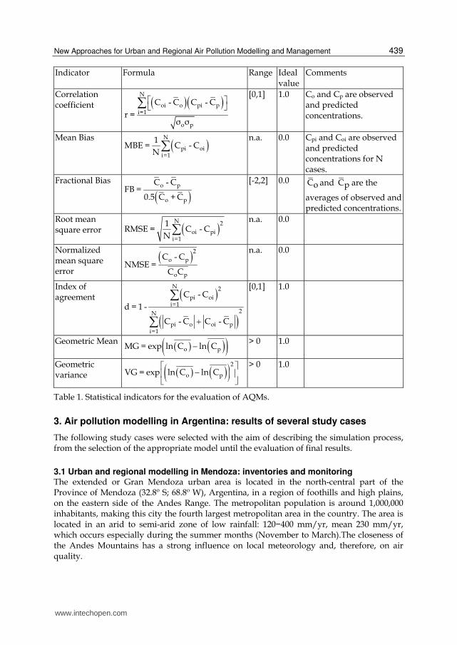
propose some statistical performance measures. Table 1 summarizes these commonly used

statistical tools for analysing and comparing model results versus measurements.

www.intechopen.com


439

Indicator Formula Range Ideal value

Comments

Correlation coefficient ( )( )N

oi o pi pi=1

o p

C - C C - C

r =σ σ

⎡ ⎤⎣ ⎦∑

[0,1] 1.0 Co and Cp are observed and predicted concentrations.

Mean Bias ( )N

pi oii=1

1MBE = C - C

N∑

n.a. 0.0 Cpi and Coi are observed and predicted concentrations for N cases.

Fractional Bias ( )o p

o p

C - CFB =

0.5 C + C

[-2,2] 0.0 Co and Cp are the

averages of observed and predicted concentrations.

Root mean square error ( )N 2

oi pii=1

1RMSE = C - C

N∑

n.a. 0.0

Normalized mean square error

( )2o p

o p

C - CNMSE =

C C

n.a. 0.0

Index of agreement ( )

( )N 2

pi oii=1

2N

pi o oi pi=1

C - C

d = 1 -

C - C C - C+∑

∑[0,1] 1.0

Geometric Mean ( ) ( )( )o pMG = exp ln C ln C− > 0 1.0

Geometric variance ( ) ( )( )2

o pVG = exp ln C ln C⎡ ⎤−⎢ ⎥⎣ ⎦

> 0 1.0

Table 1. Statistical indicators for the evaluation of AQMs.

3. Air pollution modelling in Argentina: results of several study cases

The following study cases were selected with the aim of describing the simulation process, from the selection of the appropriate model until the evaluation of final results.

3.1 Urban and regional modelling in Mendoza: inventories and monitoring The extended or Gran Mendoza urban area is located in the north-central part of the Province of Mendoza (32.8º S; 68.8º W), Argentina, in a region of foothills and high plains, on the eastern side of the Andes Range. The metropolitan population is around 1,000,000 inhabitants, making this city the fourth largest metropolitan area in the country. The area is located in an arid to semi-arid zone of low rainfall: 120−400 mm/yr, mean 230 mm/yr, which occurs especially during the summer months (November to March).The closeness of the Andes Mountains has a strong influence on local meteorology and, therefore, on air quality.

www.intechopen.com


440

Air quality in the area under study is affected by intensive and intermediate industrial

activities, emissions due to transportation, residential sources and, to a lesser degree,

agriculture and animal husbandry (Puliafito et al., 2003). Food and wine industry are very

low energy consumers, but alloys, cement and petrochemical industries are relevant to

energy consumption and their contribution to total emissions is important. Transportation is

the second most important source of pollutants in the emission inventory, but the main

concern in the downtown area. The emissions by the residential sector are mainly due to the

use of natural gas for heating. Animal husbandry is concentrated in the South East of the

Province and its contribution to total emission is low.

3.1.1 Modelling approaches The impact of all anthropogenic sources in the air quality of the urban centre was evaluated

using two different approaches: a) to reproduce the pollutant dispersion in the metropolitan

area, we chose CALPUFF modelling system, setting the modelling domain in the urban area

of Gran Mendoza; and b) to evaluate the impact of regional circulation in tropospheric

chemistry, we used WRF/Chem in a greater modelling domain.

3.1.2 Urban pollutant dispersion The modelling domain covers an area of 41×36 km2 (32.8° S to 33.1° S and 68.8° W to 69.0° W)

including the urban zone and part of the Andes. Because of the complex topography,

detailed terrain features were incorporated using the USGS global 3 arc-sec SRTM3 data

(~ 90m resolution). The LULC data was obtained from the Global Land Cover

Characterization (GLCC) database captured by a 1-km resolution. Finer features of land use

were obtained using the soil classification from the EcoAtlas Program from Mendoza’s

Rural Development Institute (IDR), which includes the interpretation and classification of

Landsat images during the year 2006. Surface and upper meteorological data was obtained

from the National Weather Service at the local airport station El Plumerillo (32.78° S, 68.78°

W, 704 m above sea level) located at 6 km North-East of the urban center. Fig. 3 shows a

view of the modelling domain. Industrial sources are located in two industrial areas in the

periphery of the city. The position and emission rates for the industrial stacks are known,

measured and compiled by the local environmental authority. Twenty one fixed (point)

sources at constant rates for the modelling period were considered. Emissions from

residential and commercial sources were estimated using data of natural gas consumption

in the city and spatially distributed according to the land-use maps of the urban center.

A top-down approach (macro scale) associated to GIS was used to calculate mobile source

emissions and their spatial distribution. The COPERT III model (Ntziachristos et al., 2000)

was selected to estimate road transport emissions because of the similarities between the

Argentinean and the European fleets (D'Angiola et al., 2010). Emission factors for Natural

Gas Vehicles (NGV) were derived from local studies (ARPEL, 2005). The vehicle fleet was

arranged into 4 vehicle classes and 28 technology categories depending on fuel type, vehicle

size, fuel delivery system and exhaust control system; 19 of these categories, belong to light

duty vehicles and passenger cars, 6 to heavy duty vehicles and 3 to urban buses.

Information from the National Vehicle Registration Directory (DNRPA) and the Automobile

Manufacturers Association (ADEFA) was used to determine the fleet composition. To derive

www.intechopen.com


441

Fig. 3. Geographical location of the City of Mendoza (left) and terrain elevations (metres a.s.l.) in the modelling domain (right).

emission rates, the model considers different average speeds for different types of driving

conditions. Three driving conditions were associated with specific road hierarchies:

a) Highways: roads characterized as main intra-county, suburban areas or inter-regional

highways connecting main town poles in the metropolitan area, with high traffic, no traffic

lights and high average speed (70-100 km/h); b) Primary roads: roads that are main streets

connecting important urban districts, with a high vehicle density, with most intersections

regulated by traffic lights, and a low average speed (20-30 km/h); c) Secondary roads: roads

that are mainly residential streets with a low vehicle density, very few or no traffic lights

regulating intersections, although, in some cases, with the presence of speed limiters and a

low–medium average speed (25-35 km/h). Average speed on each road hierarchy and

annual average kilometres traveled (VKT) were estimated from information collected on a

set of vehicles equipped with a Global Positioning Satellite (GPS) unit. The total amount of

emissions estimated for highways, primary roads and secondary roads was distributed in

the road network proportionally to the length of segments. Then, these emissions were

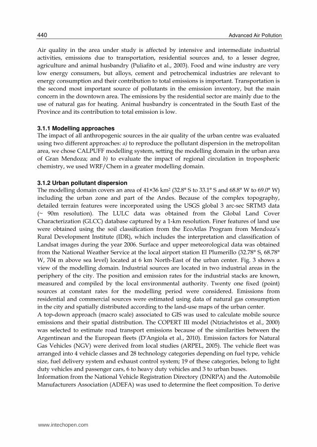
geographically distributed into a gridded map with cells of 500 m x 500 m (Fig. 4, left).

Fig. 4 (right) depicts the daily mean ambient PM10 concentration modeled with CALPUFF. It

shows concentrations of (70−80 µg/m3) in downtown area, mainly produced by mobile

sources. These values reduce towards the periphery of the city. The south-western area of

the modelling domain is greatly influenced by the industrial complex located in the south

western area of the city. PM10 emissions from dust sources were estimated according to

OAQPS (1977) and modeled as area sources in CALPUFF. The emissions were incorporated

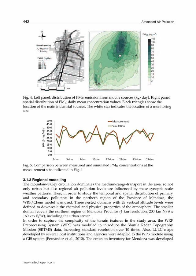
as a discontinuous process when wind speeds were above a threshold of 6.8 m/s. Fig. 5

shows a time series comparison of the modeled results versus the PM10 measurements at the

monitoring station in downtown for June 2009. Despite some peak values due to high traffic

density the results show a good correlation between modelled concentration and measured

data. A more detailed analysis of pollutant distribution in the metropolitan area of Mendoza

can be found in Puliafito & Allende (2007) and Puliafito et al. (2011).

www.intechopen.com


442

Fig. 4. Left panel: distribution of PM10 emission from mobile sources (kg/day). Right panel: spatial distribution of PM10 daily mean concentration values. Black triangles show the location of the main industrial sources. The white star indicates the location of a monitoring site.

0.0

5.0

10.0

15.0

20.0

25.0

30.0

35.0

40.0

45.0

50.0

1-Jun 5-Jun 9-Jun 13-Jun 17-Jun 21-Jun 25-Jun 29-Jun

PM

10

(u

g/m

3)

Measurement

Simulation

Fig. 5. Comparison between measured and simulated PM10 concentrations at the measurement site, indicated in Fig. 4.

3.1.3 Regional modelling The mountain-valley circulation dominates the medium-range-transport in the area, so not only urban but also regional air pollution levels are influenced by these synoptic scale weather patterns. Then, in order to study the temporal and spatial distribution of primary and secondary pollutants in the northern region of the Province of Mendoza, the WRF/Chem model was used. Three nested domains with 28 vertical altitude levels were defined to downscale the chemical and physical properties of the atmosphere. The smaller domain covers the northern region of Mendoza Province (4 km resolution, 200 km N/S x 160 km E/W), including the urban center. In order to capture the complexity of the terrain features in the study area, the WRF Preprocessing System (WPS) was modified to introduce the Shuttle Radar Topography Mission (SRTM3) data, increasing standard resolution over 10 times. Also, LULC maps developed by several local institutions and agencies were adapted to the WPS module using a GIS system (Fernandez et al., 2010). The emission inventory for Mendoza was developed

www.intechopen.com


443

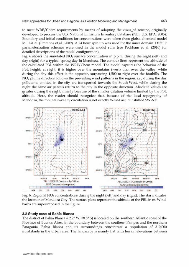
to meet WRF/Chem requirements by means of adapting the emiss_v3 routine, originally developed to process the U.S. National Emissions Inventory database (NEI; U.S. EPA, 2005). Boundary and initial conditions for concentrations were taken from global chemical model MOZART (Emmons et al., 2009). A 24 hour spin up was used for the inner domain. Default parameterization schemes were used in the model runs (see Peckham et al. (2010) for detailed descriptions of the model configuration). Fig. 6 shows the simulated NO2 surface concentration in p.p.m. during the night (left) and day (right) for a typical spring day in Mendoza. The contour lines represent the altitude of the calculated PBL within the WRF/Chem model. The model captures the behavior of the PBL height: at night, it is higher over the mountains (west) than over the valley, while during the day this effect is the opposite, surpassing 1,500 m right over the foothills. The NO2 plume direction follows the prevailing wind patterns in the region, i.e., during the day pollutants emitted in the city are transported towards the South-West, while during the night the same air parcels return to the city in the opposite direction. Absolute values are greater during the night, mainly because of the smaller dilution volume limited by the PBL altitude. Here, the reader should recognize that, because of the local topography of Mendoza, the mountain-valley circulation is not exactly West-East, but shifted SW-NE.

Fig. 6. Regional NO2 concentrations during the night (left) and day (right). The star indicates the location of Mendoza City. The surface plots represent the altitude of the PBL in m. Wind barbs are superimposed in the figure.

3.2 Study case of Bahía Blanca The district of Bahía Blanca (62.2° W; 38.5° S) is located on the southern Atlantic coast of the Province of Buenos Aires, in the boundary between the southern Pampas and the northern Patagonia. Bahía Blanca and its surroundings concentrate a population of 310,000 inhabitants in the urban area. The landscape is mainly flat with terrain elevations between

www.intechopen.com


444

200 m and 500 m, except for the low mountain system of “Sierra de la Ventana”, which reaches an altitude of 1,200 m. The area is located in a temperate zone with warm continental type weather. Its annual precipitation is about 600 mm, with high monthly variations. March, September, October and November are the months with higher probability of rainfall episodes. Winds are generally moderate, with predominant direction from North or Northwest. Mean wind speed is 5.3 m/s, with 3 % calms. Bahía Blanca has an important seaport system handling intense industrial and commercial activities. The city has a highly developed oil refinery and petrochemical industries, producing ethanol, naphtha, gasoline, asphalt GLP, ethylene, PVC, polyethylene, urea, ammonia, chlorine and caustic soda. An important power station is located outside the industrial zone, SW of the urban centre, in the port area, which may operate with natural gas or heavy–oil, producing the main contribution of SO2 emissions in the zone. Along the north-eastern shore of the bay, there are several small seaports dedicated to grains and containers. The ambient concentration of gases like NOx, CO, NH3 and SO2 and concentrations of particulate matter have been measured by the local environmental authority since 1997.

Fig. 7. Map of Argentina showing location of the modelling domain. To the right, a detail of the urban area of Bahia Blanca, major highways, the industrial complex, and the port area.

In order to complement the information provided by the monitoring data, pollutant dispersion was simulated with the CALPUFF modeling system. The modelling domain covered an area of 1,600 km2 between 38.5º and 39.0º S latitude and 62.0º and 62.5 W longitude in a flat region with elevations up to 150 m, increasing to the NE. A view of the modelling domain is presented in Fig. 7. All industrial sources are located on a Petrochemical Pole, an Industrial Park and the port sector and were treated as point sources in CALPUFF. Emissions of NOx, SO2 and NH3 due to transportation (including road, railway and ships) were estimated following the top-down emission model COPERT III similarly to the Mendoza study case. Cargo oriented railway transportation emissions were estimated using specific fuel consumption factors and a number of train operations, while maritime activity emissions were calculated using a number of operations, port waiting time and bulk

www.intechopen.com


445

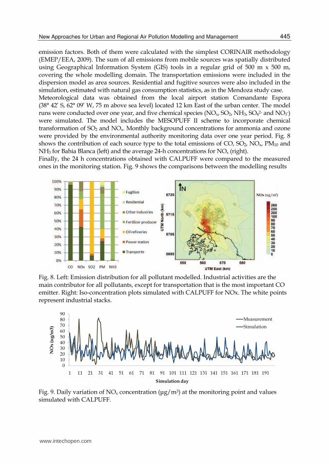
emission factors. Both of them were calculated with the simplest CORINAIR methodology (EMEP/EEA, 2009). The sum of all emissions from mobile sources was spatially distributed using Geographical Information System (GIS) tools in a regular grid of 500 m x 500 m, covering the whole modelling domain. The transportation emissions were included in the dispersion model as area sources. Residential and fugitive sources were also included in the simulation, estimated with natural gas consumption statistics, as in the Mendoza study case. Meteorological data was obtained from the local airport station Comandante Espora (38° 42’ S, 62° 09’ W, 75 m above sea level) located 12 km East of the urban center. The model runs were conducted over one year, and five chemical species (NOx, SO2, NH3, SO42- and NO3-) were simulated. The model includes the MESOPUFF II scheme to incorporate chemical transformation of SO2 and NOx. Monthly background concentrations for ammonia and ozone were provided by the environmental authority monitoring data over one year period. Fig. 8 shows the contribution of each source type to the total emissions of CO, SO2, NOx, PM10 and NH3 for Bahia Blanca (left) and the average 24-h concentrations for NOx (right). Finally, the 24 h concentrations obtained with CALPUFF were compared to the measured ones in the monitoring station. Fig. 9 shows the comparisons between the modelling results

Fig. 8. Left: Emission distribution for all pollutant modelled. Industrial activities are the main contributor for all pollutants, except for transportation that is the most important CO emitter. Right: Iso-concentration plots simulated with CALPUFF for NOx. The white points represent industrial stacks.

0102030405060708090

1 11 21 31 41 51 61 71 81 91 101 111 121 131 141 151 161 171 181 191

NO

x (u

g/m

3)

Simulation day

Measurement

Simulation

Fig. 9. Daily variation of NOx concentration (μg/m3) at the monitoring point and values simulated with CALPUFF.

www.intechopen.com


446

and the observations near the industrial complex. Although the model is unable to reproduce the concentration peaks exactly, the values of the statistical measures (MBE: -2.02; FB: -0.04; Willmott’s d: 0.97) suggest that the dispersion simulation approaches the concentrations patterns with acceptable accuracy. The modelling results showed that the most polluted region is the town of Ingeniero White, located to the SE of the metropolitan area, and very close to the Petrochemical Pole (see detailed analysis in Puliafito & Allende (2007) and Allende et al. (2010a)). The fair agreement between concentrations measured by the environmental authority over one year and the simulated ones with CALPUFF validated the proposed emissions and dispersion models.

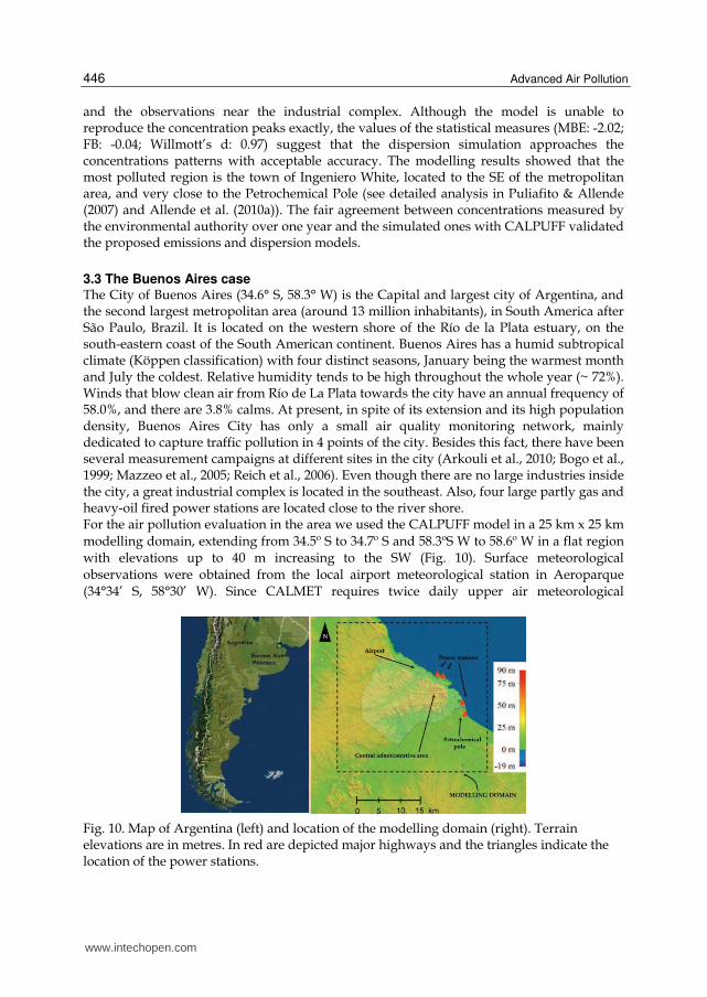
3.3 The Buenos Aires case The City of Buenos Aires (34.6° S, 58.3° W) is the Capital and largest city of Argentina, and the second largest metropolitan area (around 13 million inhabitants), in South America after São Paulo, Brazil. It is located on the western shore of the Río de la Plata estuary, on the south-eastern coast of the South American continent. Buenos Aires has a humid subtropical climate (Köppen classification) with four distinct seasons, January being the warmest month and July the coldest. Relative humidity tends to be high throughout the whole year (~ 72%). Winds that blow clean air from Río de La Plata towards the city have an annual frequency of 58.0%, and there are 3.8% calms. At present, in spite of its extension and its high population density, Buenos Aires City has only a small air quality monitoring network, mainly dedicated to capture traffic pollution in 4 points of the city. Besides this fact, there have been several measurement campaigns at different sites in the city (Arkouli et al., 2010; Bogo et al., 1999; Mazzeo et al., 2005; Reich et al., 2006). Even though there are no large industries inside the city, a great industrial complex is located in the southeast. Also, four large partly gas and heavy-oil fired power stations are located close to the river shore. For the air pollution evaluation in the area we used the CALPUFF model in a 25 km x 25 km

modelling domain, extending from 34.5º S to 34.7º S and 58.3ºS W to 58.6º W in a flat region with elevations up to 40 m increasing to the SW (Fig. 10). Surface meteorological observations were obtained from the local airport meteorological station in Aeroparque (34°34’ S, 58°30’ W). Since CALMET requires twice daily upper air meteorological

Fig. 10. Map of Argentina (left) and location of the modelling domain (right). Terrain elevations are in metres. In red are depicted major highways and the triangles indicate the location of the power stations.

www.intechopen.com


447

observations for dispersion simulating, and since observations with such frequency are not

available for this site, the required meteorological parameters were derived from the

Weather Research and Forecasting model. The CALWRF off-line preprocessor was used to

generate an intermediate three dimensional data file to be used by CALMET as a “first-

guess” meteorological field. The WRF model was run with nested domains, reaching a

resolution of 3 km, high enough to resolve the important meteorological features which can

only be simulated by the prognostic WRF model, such as land and sea breezes.

Emissions from the power stations were estimated using emission factors of CORINAIR

(EMEP/EEA, 2009) for most pollutants and IPCC (IPCC, 2006) for greenhouse gases,

according to their thermal capacity and use of fuel. The emissions from oil refineries,

chemical industries and storage tanks located very close to the city, near the SE border, were

previously measured and included directly in the CALPUFF model. All these emissions

were associated to 54 point sources. Temporal allocation of emissions was estimated using

statistical data from the local Electricity Regulation Office and gross domestic product

evolution for the industrial sector.

Emissions of NOx, SO2 and CO due to transportation were estimated following the

top-down emission model COPERT III similar to the study cases of Mendoza and Bahía

Blanca (Perez Gunella et al., 2009). Daily and monthly variation of road traffic in the city is

often measured, with traffic rush hours during working days being from 08:00 to 09:00 a.m.

and from 07:00 to 09:00 p.m. These emissions were geographically distributed into a gridded

map with cells of 300 m x 300 m (Fig. 11, right).

Fig. 11. Left: Emission contributions for all pollutants simulated in the study area. Right: Spatial allocation for NOx traffic emissions in the city of Buenos Aires.

Residential emissions were associated with natural gas and LPG consumption, and

estimated using emission factors from CORINAIR. Spatial allocation of the emissions was

made proportional to the population density in the city districts and further weighted with

the Unsatisfied Basic Needs index (NBI) to account for the population socioeconomic levels.

The emission distribution from all sources is shown in Fig. 11 (left), and concentration

patterns obtained with CALPUFF are shown in Fig. 12.

SO2 concentration maxima are clearly located near the power stations. The road traffic

appears to be responsible for high NOx values near major roadways (Puliafito et al., 2010;

Allende et al., 2010b). Monitoring values obtained in a toll gate located in the south of the

city were compared to simulated ones. For CO, the comparison is shown in Fig. 13.

www.intechopen.com


448

Fig. 12. 24 h average iso-concentration plots simulated with CALPUFF for NOx and SO2.

0

0.5

1

1.5

2

2.5

1 6 11 16 21 26 31 36 41 46 51 56 61 66 71 76 81 86 91 96

CO

(p

pm

)

Hours

Measurement

Simulation

Fig. 13. Hourly variation of CO concentration (p.p.m.) at the monitoring point and values simulated with CALPUFF.

4. Summary and concluding remarks

The purpose of this chapter was to provide an overview of several modelling tools available for air quality evaluation, providing general and prescriptive but also flexible recommendations toward the adoption of best practice. Air Quality Models (AQMs) are mathematical tools that simulate the physical and chemical processes that involve air pollutants as they disperse and react in the atmosphere. The use of AQMs improve the limitations faced by the use of the monitoring network approach by providing prediction of the temporal and spatial distribution of actual pollution levels. Modelling studies, in combination with air quality monitoring are essential and complementary tools for long and short term air pollution control strategies. A well calibrated model is a unique tool that allows the representation of the atmosphere dynamics and chemistry, including real conditions and atmospheric disturbances. From a theoretical standpoint, AQMs were divided in short-range Gaussian models (ISC3, AERMOD), advanced urban models (CALPUFF) and complex Chemical Transport Models coupled to mesoscale atmospheric models (WRF/Chem). The greatest differences between the model types are the meteorological input required, computer resources and user experience. For each of these models, we have discussed the configurations, data requirements, applicability and some physical and chemical formulations. We have identified several important aspects for selecting the proper AQM model: a) identification of

www.intechopen.com


449

the proper scale problem; b) the availability of meteorological data; c) the preparation of emission inventories; d) the inclusion of land use and topographical information; e) the integration of results in an adequate geographical information system; and finally f) a comparison of the simulated data to existing monitoring information, if any. From a practical point of view, and following the above scheme, the three study cases presented at the end of this chapter give practical implications for the selection of an AQM applied to different data availability, scale, topography and meteorology. We have described how to prepare the emission inventories for each case, and used local and regional AQMs to calculate the pollutant concentration. The acceptable accordance between the simulated concentrations and the monitored data confirms the proposed methodology described in this chapter. Finally, we hope, this chapter encourages readers to use “state of the art” models since they provide the most realistic representation of the phenomena involved in the fate of pollutants released to the atmosphere.

4. Acknowledgements

We thank the authorities of the National Technological University of Argentina (UTN) and the Argentine Research Council (CONICET) for their support in our research activities. We further thank the Argentine National Weather Service (Servicio Meteorológico Nacional, SMN) for the availability of the meteorological data. This research was supported partially by grant PICT2005 # 23-32686 from the National Science Agency (Agencia Nacional de Promoción Científica y Tecnológica, ANPCyT).

5. References

Allende, D. G., Castro, F. H., & Puliafito, S. E. (2010a). Air Pollution Characterization and

Modeling of an Industrial Intermediate City. International Journal of Applied

Environmental Sciences, 5(2), 275-296.

Allende, D. G., Cremades, P., Puliafito, Enrique, Fernandez, R. P., & Perez Gunella, F.

(2010b). Estimación de un Factor de Riesgo de Exposición a la Contaminación

Urbana par ala población de la Ciudad de Buenos Aires. Avances en Energías

Renovables y Medio Ambiente, 14, 127-134.

Arkouli, M., Ulke, A. G., Endlicher, W., Baumbach, G., Schultz, Eckart, Vogt, U., et al. (2010).

Distribution and temporal behavior of particulate matter over the urban area of

Buenos Aires. Atmospheric Pollution Research, 1(1), 1-8.

ARPEL. (2005). Medición de emisiones de vehículos en servicio en San Pablo, Santiago y

Buenos Aires. Informe Ambiental ARPEL Número 25-2005.

Ballesta, P. P., Field, R. A., Fernandez-Patier, R., Madruga, D. G., Connolly, R., Caracena, A.

B., et al. (2008). An approach for the evaluation of exposure patterns of urban

populations to air pollution. Atmospheric Environment, 42(21), 5350-5364.

Bieser,J., Aulinger,A., Matthias,V., Quante, M., & Builtjes,P. (2010). SMOKE for Europe -

adaptation, modification and evaluation of a comprehensive emission model for

Europe. Geoscientific Model Development Discussions., 3, 949-1007.

www.intechopen.com


450

Binkowski, F. S., & Roselle, S. J. (2003). Models-3 Community Multiscale Air Quality

(CMAQ) model aerosol component 1. Model description. Journal of Geophysical

Research - Atmospheres, 108(D6), 4183.

Bogo, H., Negri, R. M., & Roman, E. S. (1999). Continuous measurement of gaseous

pollutants in Buenos Aires city. Atmospheric Environment, 33(16), 2587-2598.

Borge, R., Lumbreras, J., & Rodriguez, E., 2008, Development of a high-resolution emission

inventory for Spain using the SMOKE modelling system: A case study for the years

2000 and 2010. Environmental Modelling and Software, 23, 1026–1044.

Brunekreef, B., & Holgate, S. T. (2002). Air pollution and health. Lancet, 360(9341), 1233-42.

Carter, W. P. L. (2000).Documentation of the SAPRC-99 Chemical Mechanism for VOC

Reactivity Assessment. Report to the California Air Resources Board, Available at

http://cert.ucr.edu/~carter/absts.htm#saprc99

Cimorelli, A. J., Venkatram, A., Weil, J. C., Paine, R., Wilson, R., Lee, R., et al. (2003).

AERMOD : Description of model formulation. Environmental Protection Agency.

Davis, N., Lents, J., Osses, M., Nikkila, N., & Barth, M. (2005). Development and Application

of an International Vehicle Emissions Model. Transportation Research Record, 51-59.

Demuzere, M., Trigo, R. M., Arellano, J. V.-guerau D., & Lipzig, N. P. M. V. (2009). The

impact of weather and atmospheric circulation on O3 and PM10 levels at a rural

mid-latitude site. Atmospheric Chemistry and Physics, 9, 2695-2714.

Dodge, M. C. (2000). Chemical oxidant mechanisms for air quality modeling: critical review.

Atmospheric Environment, 34(12-14), 2103-2130.

D’Angiola, A., Dawidowski, L. E., Gomez, D. R., & Osses, M. (2010). On-road traffic

emissions in a megacity. Atmospheric Environment, 44(4), 483-493.

EMEP/EEA. (2009). EMEP/EEA Air Pollutant Emission Inventory Guidebook — 2009.

Technical guidance to prepare national emission inventories. Copenhagen.

Available from: www.eea.europa.eu/help/infocentre/enquiries

Emmons, L., Walters, S., Hess, P. G., Lamarque, J., Pfister, G. G., Fillmore, D., et al. (2009).

Description and evaluation of the Model for Ozone and Related chemical Tracers,

version 4 (MOZART-4). Geosci. Model Dev. Discuss., 2, 1157-1213. Max-Planck-

Institute for Meteorology, Hamburg, Germany.

Endlicher, W., Zahnen, B., Schultz, E., Alessandro, M., Mikkan, R., & Polimeni, M. (1998).

Clima Urbano y Contaminación Atmosférica en Mendoza/Argentina. In : Clima y

Ambiente Urbano en Ciudades Ibéricas e Iberoamericanas (pp. 115-134). Madrid.

Fenger, J. (1999). Urban air quality. Atmospheric Environment, 33(29), 4877-4900.

Fernandez, R., Allende, D., Castro, F., Cremades, P., Puliafito, E. (2010). Modelado regional

de la calidad de aire utilizando el modelo WRF/Chem : implementación de datos

globales y locales para Mendoza. Avances en Energías Renovables y Medio Ambiente,

14, 01.43-01.50.

Ferretti, M., Andrei, S., Caldini, G., Grechi, D., Mazzali, C., Galanti, E., et al. (2008).

Integrating monitoring networks to obtain estimates of ground-level ozone

concentrations -- A proof of concept in Tuscany (central Italy). Science of the Total

Environment, 396(2-3), 180-192.

Fowler, D., Pilegaard, K., Sutton, M. A., Ambus, P., Raivonen, M., Duyzer, J., et al. (2009).

Atmospheric composition change: Ecosystems-Atmosphere interactions.

Atmospheric Environment, 43(33), 5193-5267.

www.intechopen.com


451

Freitas, S.R., Longo, K.M., Alonso,M.F., Pirre, M., Marecal, V., Grell, G., Stockler,R., Mello,

R.F., & Sánchez Gácita,M.. (2010). A pre-processor of trace gases and aerosols

emission fields for regional and global atmospheric chemistry models. Geoscientific

Model Development Discussions, 3, 855-888.

GEIA/ACCENT. (2005). GEIA-ACCENT database, an international cooperative activity of

AIMES/IGBP. ACCENT EU Network of Excellence. http://www.geiacenter.org

Gery, M.W., Whitten, G.Z., Killus, J.P. & Dodge, M.C. (1989). A photochemical kinetics

mechanism for urban and regional scale computer modeling. Journal of Geophysical

Research, 94, 1292-12956.

Gilliland, A. B., Hogrefe, C., Pinder, R. W., Godowitch, J. M., Foley, K. L., & Rao, S. T. (2008).

Dynamic evaluation of regional air quality models: Assessing changes in O3

stemming from changes in emissions and meteorology. Atmospheric Environment,

42(20), 5110-5123.

Grell, G. A, Peckham, S. E., Schmitz, Rainer, McKeen, S. a, Frost, G., Skamarock, W. C., et al.

(2005). Fully coupled “online” chemistry within the WRF model. Atmospheric

Environment, 39(37), 6957-6975.

Hanna, S. R., Lu, Z., Frey, H. C., Wheeler, N., Vukovich, J., Arunachalam, S., et al. (2001).

Uncertainties in predicted ozone concentrations due to input uncertainties for the

UAM-V photochemical grid model applied to the July 1995 OTAG domain.


IPCC. (2006). 2006 IPCC Guidelines for National Greenhouse Gas Inventories. Hayama,

Kanagawa, Japan. Available from http://ipcc-nggip.iges.or.jp

Jiménez-Guerrero, P., Jorba, O., Baldasano, J. M., & Gassó, S. (2008). The use of a modelling

system as a tool for air quality management: annual high-resolution simulations

and evaluation. The Science of the Total Environment, 390(2-3), 323-40.

Leeuw, F. A. A. M. de, Moussiopoulos, N., Sahm, P., & Bartonova, A. (2001). Urban air

quality in larger conurbations in the European Union. Environmental Modelling &

Software, 16(4), 399-414.

Martin, R. V. (2008). Satellite remote sensing of surface air quality. Atmospheric Environment,

42(34), 7823-7843.

Mazzeo, N. A., Venegas, L. E., & Choren, H. (2005). Analysis of NO, NO2, O3 and NOx

concentrations measured at a green area of Buenos Aires City during wintertime.


Michalakes, J., Dudhia, J., Gill, D., Henderson, T., Klemp, J., Skamarock, W., et al. (2005). the

Weather Research and Forecast Model: Software Architecture and Performance. Use of High Performance Computing in Meteorology - Proceedings of the Eleventh

ECMWF Workshop, (June), 156-168. Singapore: World Scientific Publishing Co.

Muller, N. Z., & Mendelsohn, R. (2007). Measuring the damages of air pollution in the

United States. Journal of Environmental Economics and Management, 54(1), 1-14.

Ntziachristos, L., Samaras, Z., & Kouridis, C. (2000). COPERT III Computer programme to

calculate emissions from road transport. Copenhagen.

OAQPS. (1977). Guideline for development of control strategies in areas with fugitive dust

problems. EPA-405/2- 77-029.

www.intechopen.com


452

Olivier, J. G. J., & Berdowski, J. J. M. (2001). Global emissions sources and sinks. Berdowski, J.,

Guicherit, R. and B.J. Heij (eds.) "The Climate System" (pp. 33-78). Lisse, The

Netherlands. A.A. Balkema Publishers/Swets & Zeitlinger Publishers.

Oxley, T., Valiantis, M., Elshkaki, a, & ApSimon, H. M. (2009). Background, Road and Urban

Transport modelling of Air quality Limit values (The BRUTAL model).

Environmental Modelling & Software, 24(9), 1036-1050.

Pearce, J. L., Beringer, J., Nicholls, N., Hyndman, R. J., Uotila, P., & Tapper, N. J. (2011).

Investigating the influence of synoptic-scale meteorology on air quality using self-

organizing maps and generalized additive modelling. Atmospheric Environment,

45(1), 128-136.

Peckham, S., Grell, G., McKeen, S., Fast, J., Gustafson, W., Ghan, S., et al. (2010). WRF/Chem

Version 3.2 User’s Guide. Available from

http://ruc.noaa.gov/wrf/WG11/Users_guide.pdf

Perez Gunella, F., Puliafito, S.E., & Pirani, K. (2009). Calculo de las emisiones del transporte

para la Ciudad de Buenos Aires usando un Sistema de Informacion Geografico.

Avances en Energías Renovables y Medio Ambiente, 13, 57-64.

Puliafito, E, Guevara, M., & Puliafito, C. (2003). Characterization of urban air quality using

GIS as a management system. Environmental pollution, 122(1), 105-17.

Puliafito, E., & Allende, D. G. (2007). Emission patterns of urban air pollution. Revista

Facultad de Ingeniería Universidad de Antioquia, 42, 38-56.

Puliafito, E., Castro, F., & Allende, D. G. (2011). Air quality impact of PM10 emission in

urban centers. International Journal of Environment and Pollution, (in press).

Puliafito, E., Perez Gunella, F., & Allende, D. G. (2010). Modelo de Calidad del Aire para la

Ciudad de Buenos Aires. World Congress & Exhibition ENGINEERING 2010-

ARGENTINA. Buenos Aires, Argentina.

Reich, S., Magallanes, J., Dawidowski, L., Gómez, D., Grošelj, N., & Zupan, J. (2006). An

Analysis of Secondary Pollutants in Buenos Aires City. Environmental Monitoring

and Assessment, 119(1), 441-457. Springer Netherlands.

Russell, A., & Dennis, R. (2000). NARSTO critical review of photochemical models and

modeling. Atmospheric Environment, 34(12-14), 2283-2324.

Schlink, U., Herbarth, O., Richter, M., Rehwagen, M., Puliafito, J. L., Puliafito, S. E., et al.

(1999). Ozone-monitoring in Mendoza, Argentina : Initial results. Journal of the Air

& Waste Management Association, 49(1), 82-87.

Schürmann, G. J., Algieri, A., Hedgecock, I. M., Manna, G., Pirrone, N., & Sprovieri, F.

(2009). Modelling local and synoptic scale influences on ozone concentrations in a

topographically complex region of Southern Italy. Atmospheric Environment, 43(29),

4424-4434.

Schultz, M. G., Backman, L., Balkanski, Y., Bjoerndalsaeter, S., Brand, R., Burrows, J. P., et al.

(2008). REanalysis of the TROpospheric chemical composition over the past 40

years. A long-term global modeling study of tropospheric chemistry funded under

the 5th EU framework programme. Final Report. (Vol. 30, pp. 281-8). Hamburg.

Scire, J. S., Strimaitis, D. G., & Yamartino, R. J. (2000a). A User’s Guide for the CALPUFF

Dispersion Model. Concord, MA.

Scire, J. S., Robe, F. R., Fernau, M. E., & Yamartino, R. J. (2000b). A User’s Guide for the

CALMET Meteorological Model. Concord, MA.

www.intechopen.com


453

Seaman, N. L. (2003). Future directions of meteorology related to air-quality research.

Environment International, 29(2-3), 245-252.

Seigneur, C., Pun, B., Pai, P., Louis, J., Solomon, P. A., Emery, C., et al. (2000). Guidance for

the Performance Evaluation of Three-Dimensional Air Quality Modeling Systems

for Particulate Matter and Visibility. Journal of the Air & Waste Management

Association, 50(4), 588-599.

Skamarock, W. C., Klemp, J. B., Gill, D. O., Barker, D. M., Wang, W., & Powers, J. G. (2008).

A Description of the Advanced Research WRF Version 3. Mesoscale and Microscale

Meteorology Division, National Center for Atmospheric Research.

Stockwell, W. R., Middleton, P., & Chang, J. S. (1990). The second generation regional acid

deposition model chemical mechanism for regional air quality modeling. Journal of

Geophysical Research, 95, 16343-16367.

Stockwell, William R, Kirchner, F., Kuhn, M., & Seefeld, S. (1997). A new mechanism for

regional atmospheric chemistry modeling. Journal of Geophysical Research., 102(D22),

25847-25879.

Tuia D., Ossés de Eicker M., Zah R., Osses M., Zarate E., Clappier A. (200). Evaluation of a

simplified top-down model for the spatial assessment of hot traffic emissions in

mid-sized cities. Atmospheric Environment, 41, 3658–3671.

U.S. EPA. (1995). User’s Guide for the Industrial Source Complex (ISC3) Dispersion Model.

Description of model algorithms. Research Triangle Park, NC 27711.

U.S. EPA. (2000). Meteorological Monitoring Guidance for Regulatory Modeling

Applications (p. 171). Research Triangle Park, NC 27711.

U.S. EPA. (2005). 2005 National Emissions Inventory Data & Documentation. Retrieved

January 1, 2010, from http://www.epa.gov/ttn/chief/net/2005inventory.html

U.S. EPA. (2008). Technical Issues Related to use of the CALPUFF Modeling System for

Near-field Applications. Research Triangle Park, NC 27711.

U.S. EPA. (2009a). Motor Vehicle Emission Simulator (MOVES) 2010 User Guide (p. 150).

U.S. EPA. (2009a). SPECIATE 4.2 Speciation Database Development Documentation.

EPA600-R-09/038. Available at: http:/www.epa.gov/ttn/chief/software/speciate

U.S. EPA. (2010). AP 42, Fifth Edition Compilation of Air Pollutant Emission Factors.

Retrieved January 1, 2010, from http://www.epa.gov/ttnchie1/ap42/

U.S. Geological Survey (USGS). (2010). The Global Land Cover Characterization (GLCC)

Database. Available from: http://www.src.com/datasets/GLCC_Info_Page.html

Van der Werf, G. R., Randerson, J. T., Giglio, L., Collatz, G. J., Mu, M., Kasibhatla, P. S.,

Morton, D. C., DeFries, R. S., Jin, Y., & van Leeuwen, T. T. (2010). Global fire

emissions and the contribution of deforestation, savanna, forest, agricultural, and

peat fires (1997–2009), Atmospheric Chemistry and Physics Discussions., 10, 11707-

11735.

Wang, Xuemei, Wu, Z., & Liang, G. (2009). WRF/CHEM modeling of impacts of weather

conditions modified by urban expansion on secondary organic aerosol formation

over Pearl River Delta. Particuology, 7(5), 384-391.

Wang, Xueyuan, Liang, X.-Z., Jiang, W., Tao, Z., Wang, J. X. L., Liu, H., et al. (2010). WRF-

Chem simulation of East Asian air quality: Sensitivity to temporal and vertical

emissions distributions. Atmospheric Environment, 44(5), 660-669.

www.intechopen.com


454

WHO. (2002). The World Health Report 2002: Reducing Risks, Promoting Healthy Life. World

Health (p. 13). Geneva.

Willmott, C. (1982). Some Comments on the Evaluation of Model Performance. Bulletin of the

American Meteorological Society, 63, 1309-1369.

Zannetti, P. (1990). Air Pollution Modelling. Van Nostrand Reinhold. New York.

www.intechopen.com

Advanced Air PollutionEdited by Dr. Farhad Nejadkoorki

ISBN 978-953-307-511-2Hard cover, 584 pagesPublisher InTechPublished online 17, August, 2011Published in print edition August, 2011

InTech EuropeUniversity Campus STeP Ri Slavka Krautzeka 83/A 51000 Rijeka, Croatia Phone: +385 (51) 770 447 Fax: +385 (51) 686 166www.intechopen.com

InTech ChinaUnit 405, Office Block, Hotel Equatorial Shanghai No.65, Yan An Road (West), Shanghai, 200040, China

Phone: +86-21-62489820 Fax: +86-21-62489821

Leading air quality professionals describe different aspects of air pollution. The book presents information onfour broad areas of interest in the air pollution field; the air pollution monitoring; air quality modeling; the GIStechniques to manage air quality; the new approaches to manage air quality. This book fulfills the need on thelatest concepts of air pollution science and provides comprehensive information on all relevant componentsrelating to air pollution issues in urban areas and industries. The book is suitable for a variety of scientists whowish to follow application of the theory in practice in air pollution. Known for its broad case studies, the bookemphasizes an insightful of the connection between sources and control of air pollution, rather than being asimple manual on the subject.

How to referenceIn order to correctly reference this scholarly work, feel free to copy and paste the following:

Salvador Enrique Puliafito, David Allende, Rafael Ferna ́ndez, Fernando Castro and Pablo Cremades (2011).New Approaches for Urban and Regional Air Pollution Modelling and Management, Advanced Air Pollution, Dr.Farhad Nejadkoorki (Ed.), ISBN: 978-953-307-511-2, InTech, Available from:http://www.intechopen.com/books/advanced-air-pollution/new-approaches-for-urban-and-regional-air-pollution-modelling-and-management

new approaches for urban and regional air pollution ...cdn.intechweb.org/pdfs/17393.pdf · new...

Documents