new approaches to the dynamics, measurement and economic
TRANSCRIPT

Philipp Kolo
New Approachesto the Dynamics,
Measurement and EconomicImplications
of Ethnic Diversity
LA
NG
P.
Kol
o · D
ynam
ics,
Mea
sure
men
t an
d E
cono
mic
Imp
licat
ions
of E
thni
c D
iver
sity
PETER LANGInternationaler Verlag der Wissenschaften
Göttinger Studien zur EntwicklungsökonomikGöttingen Studies in Development EconomicsHerausgegeben von/ Edited by Hermann Sautter und/and Stephan Klasen
Bd./Vol. 36
36This book examines the measurement and econometric effects of ethnic di-versity. This issue is of great relevance to research and policy and is currently being discussed a great deal in the literature. In particular, a sizable literature has suggested that ethnic diversity constitutes a significant barrier to economic development. The precise measurement and interpretation of these results are a matter of substantial controversy. In this book, the dynamics of ethnic diversity are being empirically analyzed for the first time. Furthermore, it develops and applies a new measure of ethnic diversity which takes the distance between groups into account, thus focusing on diversity rather than mere fragmentation. This book convincingly confronts theoretical considerations with (new) data and thereby provides a good mix of theory and empirics, making significant contributions to the current debates.
Philipp Kolo started his studies of economics in 2001 at the Ludwig Maximilian University of Munich. After a year at the Université de Lausanne he received his diploma in 2006. After working three years in strategy consulting, the author started working on his dissertation in 2010 at the University of Göttingen. In 2012 he successfully received his doctor degree.
www.peterlang.de ISBN 978-3-631-63821-7
GSEW 36_263821_Kolo_TP_A5HC.indd 1 04.10.12 12:02:49 Uhr
Philipp Kolo - 978-3-653-02395-4Downloaded from PubFactory at 01/11/2019 11:11:06AM
via free access

Göttinger Studien zur EntwicklungsökonomikGöttingen Studies in Development Economics
Herausgegeben von/ Edited by Hermann Sautter und/and Stephan Klasen
Bd./Vol. 36
PETER LANGFrankfurt am Main · Berlin · Bern · Bruxelles · New York · Oxford · Wien
Philipp Kolo - 978-3-653-02395-4Downloaded from PubFactory at 01/11/2019 11:11:06AM
via free access

Philipp Kolo
New Approachesto the Dynamics,
Measurement and EconomicImplications
of Ethnic Diversity
PETER LANGInternationaler Verlag der Wissenschaften
Philipp Kolo - 978-3-653-02395-4Downloaded from PubFactory at 01/11/2019 11:11:06AM
via free access

Bibliographic Information published by the Deutsche Nationalbibliothek
Cover design:© Olaf Glöckler, Atelier Platen, Friedberg
D 7ISSN 1439-3395
ISBN 978-3-631-63821-7
© Peter Lang GmbHInternationaler Verlag der Wissenschaften
Frankfurt am Main 2012
www.peterlang.de
Bibliographic Information published by the Deutsche Nationalbibliothek
Cover design:© Olaf Glöckler, Atelier Platen, Friedberg
D 7ISSN 1439-3395
ISBN 978-3-631-63821-7
© Peter Lang GmbHInternationaler Verlag der Wissenschaften
Frankfurt am Main 2012
www.peterlang.de
Bibliographic Information published by the Deutsche Nationalbibliothek
Cover design:© Olaf Glöckler, Atelier Platen, Friedberg
D 7ISSN 1439-3395
ISBN 978-3-631-63821-7
© Peter Lang GmbHInternationaler Verlag der Wissenschaften
Frankfurt am Main 2012
www.peterlang.de
Bibliographic Information published by the Deutsche Nationalbibliothek
Cover design:© Olaf Glöckler, Atelier Platen, Friedberg
D 7ISSN 1439-3395
ISBN 978-3-631-63821-7
© Peter Lang GmbHInternationaler Verlag der Wissenschaften
Frankfurt am Main 2012
www.peterlang.de
The Deutsche Nationalbibliothek lists this publication in the DeutscheNationalbibliografie; detailed bibliographic data is available in the internetat http://dnb.d-nb.de.
Open Access: The online version of this publication is published on www.peterlang.com and www.econstor.eu under the international Creative Commons License CC-BY 4.0. Learn more on how you can use and share this work: http://creativecommons.org/licenses/by/4.0.
All versions of this work may contain content reproduced under license from third parties.Permission to reproduce this third-party content must be obtained from these third-parties directly.
This book is available Open Access thanks to the kind support of ZBW – Leibniz-Informationszentrum Wirtschaft.
Bibliografische Information der Deutschen Nationalbibliothek
Gedruckt mit Unterstützung der Helmut Schmidt Universität Hamburg
D 705
ISSN 1433-1519 ISBN 978-3-631-63445-5 (Print)
E-ISBN 978-3-653-05213-8 (E-Book) DOI 10.3726/978-3-653-05213-8
© Peter Lang GmbH
Internationaler Verlag der Wissenschaften Frankfurt am Main 2015
PL Academic Research ist ein Imprint der Peter Lang GmbH.
Peter Lang – Frankfurt am Main · Bern · Bruxelles · New York · Oxford · Warszawa · Wien
Diese Publikation wurde begutachtet.
www.peterlang.com
ISBN 978-3-653-02395-4 (E-Book)
(Print)DOI 10.3726/978-3-653-02395-4
Philipp Kolo - 978-3-653-02395-4Downloaded from PubFactory at 01/11/2019 11:11:06AM
via free access

Editor’s Preface
In his dissertation, Philipp Kolo examines the measurement and econometric effects ofethnic diversity. This issue is of great relevance to research and policy and is currentlybeing discussed a great deal in the literature. In particular, a sizable literature has sug-gested that ethnic diversity constitutes a significant barrier to economic development. Theprecise measurement and interpretation of these results are a matter of substantial contro-versy. This book makes significant contributions to these debates. First, the dynamics ofethnic diversity are being empirically analyzed for the first time. Second, it develops andapplies a new measure of ethnic diversity which takes the distance between groups into ac-count, thus focusing on diversity rather than mere fragmentation. Mr. Kolo convincinglyconfronts theoretical considerations with (new) data and thereby provides a good mix oftheory and empirics and valuable input to this field. These two aspects are new to thisextremely diverse area of literature and Mr. Kolo shows that he is well-aware of recentdevelopments in the field and is able to significantly contribute to it.
Chapter 1 provides the theoretical basis for the following empirical chapter 2, present-ing the first substantial analysis. Here the development of ethnic diversity over time isexplained within a model framework. Above all, the influences of education, development,trade and immigration are theoretically examined, illustrating how these factors can havean influence on the development of ethnic diversity.
In the second chapter, the level of ethnic diversity and its trends is empirically ana-lyzed. Initially, the factors influencing ethnic diversity are derived from the literature andregressions are then run. The results show that there is a ’base level’ of heterogeneity,determined by geography and evolutionary factors. Additionally, it is found that the na-ture of colonization has a particularly strong influence, while urbanization, education andimmigration are the most influential factors regarding changes in ethnic fractionalizationover time. Showing the dynamics of ethnic fractionalization empirically is a major contri-bution of this dissertation. The results here are based on the data on diversity that Mr.Kolo has discovered over the last two years and these will certainly be received with greatinterest.
In the third chapter, a new measure of ethnic diversity is then generated, which,as mentioned, takes the distance between groups into account. The so-called distanceadjusted ethno-linguistic fractionalization index (DELF) builds on an impressive amount
Philipp Kolo - 978-3-653-02395-4Downloaded from PubFactory at 01/11/2019 11:11:06AM
via free access

vi
of new data to address this issue. Mr. Kolo calculates three indices of religious, ethno-racial, and linguistic diversity, and an overall index based on these three components. Themain analysis weights the three components equally. However, the appendix reports asubstantial amount of detail on different possible weighting schemes, showing the resultsto be robust. Again, this is very well derived and almost solely based on new data. Inturn, yet another important desideratum is tackled in the literature.
Finally, in the last chapter, this measure is employed in order to replicate a numberof different analyses from the literature. In particular, the influence of ethnic diversityon conflict, growth, trust, trade and the mutual opinions of different populations towardstheir counterparts are applied. In these cases, it is shown that this measure portrays justas well, and sometimes even better effects. A genuine contribution to the literature isalso achieved here, and it is impressive to see how many studies are replicated and furtherenriched through this new measure.
Altogether this thesis provides a highly interesting and sophisticated theoretical aswell as empirical evaluation of the measurement, determinants, and consequences of eth-nic fragmentation and diversity. The fact that all four pieces break new ground in termsof methodical and empirical analysis is particularly commendable, and with this, PhilippKolo has succeeded in providing several important contributions to the literature.
Prof. Stephan Klasen (Ph.D.)Göttingen, April 2012
Philipp Kolo - 978-3-653-02395-4Downloaded from PubFactory at 01/11/2019 11:11:06AM
via free access

Acknowledgements
Bringing this dissertation to a successful end is hardly possible without the help andsupport of many people, colleagues, and friends. My deepest thanks go to my supervisors,first and foremost Prof. Stephan Klasen. Coming back to the university after several yearsworking in a business environment, I am indebted to him for giving me the opportunityto work on this dissertation, researching in a particular fascinating field. I am especiallygrateful for his continuous support and all the inspiring inputs I received. There wasnot a single point when I didn’t have the impression he had advice or a new idea readybefore I even finished my question. This agility and his diversity of knowledge was alwaysintriguing. The trust in giving me the freedom to work from long distance during mostof my research topped off his diligent supervision. I would also like to thank Prof. AxelDreher for his willingness to supervise my dissertation although he left Göttingen forHeidelberg. I benefited enormously from his inspiring comments and his responsivenesseasily compensated for the distance between us. Finally, my thanks go to Prof. WalterZucchini, who accepted the supervision, taking up his free time after retiring from activeteaching, actively engaging in further improving this dissertation.
Although I was not continuously in Göttingen, I benefited a lot from all my colleaguesat the Chair of Development Economics, and all other chairs that filled our staff seminarwith life and stimulating contributions. Even more importantly, colleagues turned intofriends, supporting me with advice and encouraging words, especially during the finalstretch. Additionally, I gained new insights from seminar participants’ helpful suggestionsand valuable comments at the DIW (Berlin) and the University of Hannover, who haddifferent perspectives on my research. The exchange and discussions with Joan Esteban,Olaf de Groot and Laura Mayoral helped to excel my results. I am especially thankful toChristian Bjørnskov, Anne-Célia Disdier, Eliana La Ferrara and Gabriel Felbermayr forsharing their data and making some of my empirical analysis possible.
Finally, sincere thanks go to my family and my friends, who always trusted and en-couraged me along this journey. Without their persistent support, successfully finishingthis project would have been much, much harder!
Philipp KoloMunich, April 2012
Philipp Kolo - 978-3-653-02395-4Downloaded from PubFactory at 01/11/2019 11:11:06AM
via free access

Philipp Kolo - 978-3-653-02395-4Downloaded from PubFactory at 01/11/2019 11:11:06AM
via free access
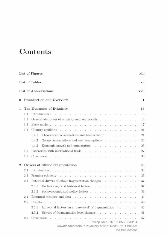
Contents
List of Figures xiii
List of Tables xv
List of Abbreviations xvii
0 Introduction and Overview 1
1 The Dynamics of Ethnicity 131.1 Introduction . . . . . . . . . . . . . . . . . . . . . . . . . . . . . . . . . . . . 131.2 General attributes of ethnicity and key models . . . . . . . . . . . . . . . . 141.3 Basic model . . . . . . . . . . . . . . . . . . . . . . . . . . . . . . . . . . . . 171.4 Country equilibria . . . . . . . . . . . . . . . . . . . . . . . . . . . . . . . . 21
1.4.1 Theoretical considerations and base scenario . . . . . . . . . . . . . 211.4.2 Group constellations and cost assumptions . . . . . . . . . . . . . . 241.4.3 Economic growth and immigration . . . . . . . . . . . . . . . . . . . 25
1.5 Extensions with international trade . . . . . . . . . . . . . . . . . . . . . . . 271.6 Conclusion . . . . . . . . . . . . . . . . . . . . . . . . . . . . . . . . . . . . 30
2 Drivers of Ethnic Fragmentation 332.1 Introduction . . . . . . . . . . . . . . . . . . . . . . . . . . . . . . . . . . . . 332.2 Framing ethnicity . . . . . . . . . . . . . . . . . . . . . . . . . . . . . . . . . 352.3 Potential drivers of ethnic fragmentation changes . . . . . . . . . . . . . . . 37
2.3.1 Evolutionary and historical factors . . . . . . . . . . . . . . . . . . . 372.3.2 Socioeconomic and policy factors . . . . . . . . . . . . . . . . . . . . 39
2.4 Empirical strategy and data . . . . . . . . . . . . . . . . . . . . . . . . . . . 432.5 Results . . . . . . . . . . . . . . . . . . . . . . . . . . . . . . . . . . . . . . . 46
2.5.1 Influential factors on a ‘base-level’ of fragmentation . . . . . . . . . 462.5.2 Drivers of fragmentation level changes . . . . . . . . . . . . . . . . . 51
2.6 Conclusion . . . . . . . . . . . . . . . . . . . . . . . . . . . . . . . . . . . . 57Philipp Kolo - 978-3-653-02395-4
Downloaded from PubFactory at 01/11/2019 11:11:06AMvia free access
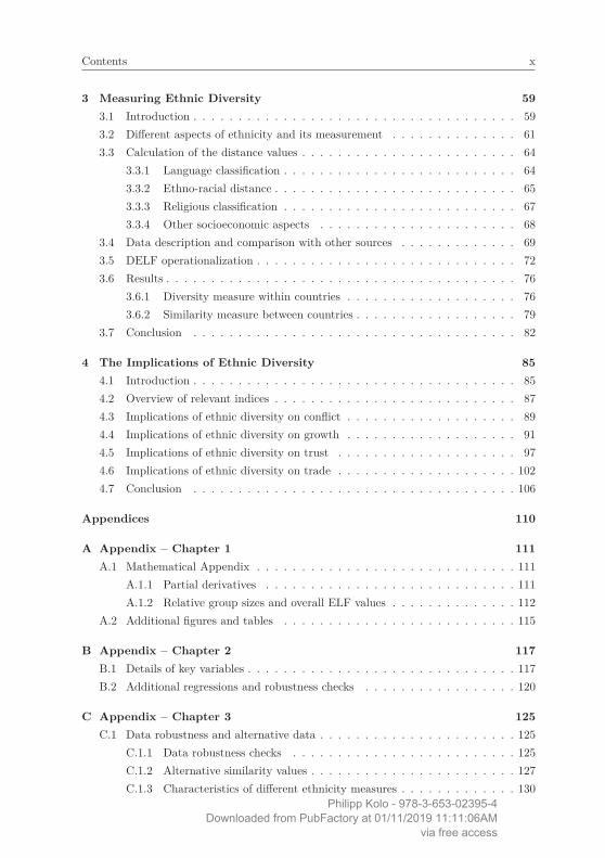
Contents x
3 Measuring Ethnic Diversity 593.1 Introduction . . . . . . . . . . . . . . . . . . . . . . . . . . . . . . . . . . . . 593.2 Different aspects of ethnicity and its measurement . . . . . . . . . . . . . . 613.3 Calculation of the distance values . . . . . . . . . . . . . . . . . . . . . . . . 64
3.3.1 Language classification . . . . . . . . . . . . . . . . . . . . . . . . . . 643.3.2 Ethno-racial distance . . . . . . . . . . . . . . . . . . . . . . . . . . . 653.3.3 Religious classification . . . . . . . . . . . . . . . . . . . . . . . . . . 673.3.4 Other socioeconomic aspects . . . . . . . . . . . . . . . . . . . . . . 68
3.4 Data description and comparison with other sources . . . . . . . . . . . . . 693.5 DELF operationalization . . . . . . . . . . . . . . . . . . . . . . . . . . . . . 723.6 Results . . . . . . . . . . . . . . . . . . . . . . . . . . . . . . . . . . . . . . . 76
3.6.1 Diversity measure within countries . . . . . . . . . . . . . . . . . . . 763.6.2 Similarity measure between countries . . . . . . . . . . . . . . . . . . 79
3.7 Conclusion . . . . . . . . . . . . . . . . . . . . . . . . . . . . . . . . . . . . 82
4 The Implications of Ethnic Diversity 854.1 Introduction . . . . . . . . . . . . . . . . . . . . . . . . . . . . . . . . . . . . 854.2 Overview of relevant indices . . . . . . . . . . . . . . . . . . . . . . . . . . . 874.3 Implications of ethnic diversity on conflict . . . . . . . . . . . . . . . . . . . 894.4 Implications of ethnic diversity on growth . . . . . . . . . . . . . . . . . . . 914.5 Implications of ethnic diversity on trust . . . . . . . . . . . . . . . . . . . . 974.6 Implications of ethnic diversity on trade . . . . . . . . . . . . . . . . . . . . 1024.7 Conclusion . . . . . . . . . . . . . . . . . . . . . . . . . . . . . . . . . . . . 106
Appendices 110
A Appendix – Chapter 1 111A.1 Mathematical Appendix . . . . . . . . . . . . . . . . . . . . . . . . . . . . . 111
A.1.1 Partial derivatives . . . . . . . . . . . . . . . . . . . . . . . . . . . . 111A.1.2 Relative group sizes and overall ELF values . . . . . . . . . . . . . . 112
A.2 Additional figures and tables . . . . . . . . . . . . . . . . . . . . . . . . . . 115
B Appendix – Chapter 2 117B.1 Details of key variables . . . . . . . . . . . . . . . . . . . . . . . . . . . . . . 117B.2 Additional regressions and robustness checks . . . . . . . . . . . . . . . . . 120
C Appendix – Chapter 3 125C.1 Data robustness and alternative data . . . . . . . . . . . . . . . . . . . . . . 125
C.1.1 Data robustness checks . . . . . . . . . . . . . . . . . . . . . . . . . 125C.1.2 Alternative similarity values . . . . . . . . . . . . . . . . . . . . . . . 127C.1.3 Characteristics of different ethnicity measures . . . . . . . . . . . . . 130
Philipp Kolo - 978-3-653-02395-4Downloaded from PubFactory at 01/11/2019 11:11:06AM
via free access

Contents xi
C.2 Details on similarity calculations, weighting and its implication for the in-terpretation of results . . . . . . . . . . . . . . . . . . . . . . . . . . . . . . 131C.2.1 Similarity matrix calculations . . . . . . . . . . . . . . . . . . . . . . 131C.2.2 Arithmetic mean . . . . . . . . . . . . . . . . . . . . . . . . . . . . . 133C.2.3 Geometric mean and partly compensating methods . . . . . . . . . . 134C.2.4 Principal component analysis . . . . . . . . . . . . . . . . . . . . . . 136C.2.5 Implications of similarity value construction . . . . . . . . . . . . . . 138C.2.6 Details of similarity interpretation between countries . . . . . . . . . 140C.2.7 Details of population weighting for regional means . . . . . . . . . . 141
C.3 Detailed DELF data per country . . . . . . . . . . . . . . . . . . . . . . . . 143
D Appendix – Chapter 4 151D.1 Summary statistics for all replications . . . . . . . . . . . . . . . . . . . . . 151D.2 Marginal effects of DELF . . . . . . . . . . . . . . . . . . . . . . . . . . . . 154
Bibliography 155
Philipp Kolo - 978-3-653-02395-4Downloaded from PubFactory at 01/11/2019 11:11:06AM
via free access

Philipp Kolo - 978-3-653-02395-4Downloaded from PubFactory at 01/11/2019 11:11:06AM
via free access

List of Figures
0.1 Difference of fragmentation and diversity measure . . . . . . . . . . . . . . . 50.2 Overview of ethnicity’s role in the economic context . . . . . . . . . . . . . 60.3 Structure of the dissertation . . . . . . . . . . . . . . . . . . . . . . . . . . . 7
1.1 Density and cost functions . . . . . . . . . . . . . . . . . . . . . . . . . . . . 231.2 Results of dynamic modeling . . . . . . . . . . . . . . . . . . . . . . . . . . 241.3 ELF values for different group constellations . . . . . . . . . . . . . . . . . . 241.4 ELF values after 15 rounds depending on θ values . . . . . . . . . . . . . . 251.5 ELF values for different growth rates . . . . . . . . . . . . . . . . . . . . . . 261.6 Overall country ELF values for different immigration rates . . . . . . . . . . 27
3.1 ELF and POL values depending on the number of groups . . . . . . . . . . 623.2 Comparison of DELF and ELF values . . . . . . . . . . . . . . . . . . . . . 763.3 Average DELF values of the EU per enlargement wave . . . . . . . . . . . 81
4.1 Scatter plot of ELF and DELF rank values . . . . . . . . . . . . . . . . . . 89
A.1 Different relative group sizes with a constant ELF . . . . . . . . . . . . . . 114A.2 Density functions for selected B(α,β) distributions . . . . . . . . . . . . . . 115A.3 Cost functions for selected levels of θ . . . . . . . . . . . . . . . . . . . . . . 115
C.1 DELF values based on random data sets . . . . . . . . . . . . . . . . . . . 126C.2 DELF values based on reduced data set . . . . . . . . . . . . . . . . . . . . 126C.3 Single characteristic skl versus linear similarity levels . . . . . . . . . . . . . 127C.4 Comparison of WCE and linear similarity values . . . . . . . . . . . . . . . 128C.5 Similarity functions depending on different concavity assumptions . . . . . . 129C.6 ELF and POL values against number of groups . . . . . . . . . . . . . . . . 130C.7 Fitted ELF and DELF values against number of groups . . . . . . . . . . . 130C.8 Scatter plots of the differently weighted DELF values . . . . . . . . . . . . 136C.9 Scatter plot for BODI and DELF values . . . . . . . . . . . . . . . . . . . 139
D.1 Average marginal effects of DELF dependent on HDI level . . . . . . . . . 154
Philipp Kolo - 978-3-653-02395-4Downloaded from PubFactory at 01/11/2019 11:11:06AM
via free access

Philipp Kolo - 978-3-653-02395-4Downloaded from PubFactory at 01/11/2019 11:11:06AM
via free access
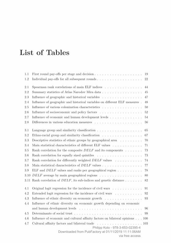
List of Tables
1.1 First round pay-offs per stage and decision . . . . . . . . . . . . . . . . . . . 191.2 Individual pay-offs for all subsequent rounds . . . . . . . . . . . . . . . . . . 22
2.1 Spearman rank correlations of main ELF indices . . . . . . . . . . . . . . . 442.2 Summary statistics of Atlas Narodov Mira data . . . . . . . . . . . . . . . . 452.3 Influence of geographic and historical variables . . . . . . . . . . . . . . . . 472.4 Influence of geographic and historical variables on different ELF measures . 482.5 Influence of various colonization characteristics . . . . . . . . . . . . . . . . 502.6 Influence of socioeconomic and policy factors . . . . . . . . . . . . . . . . . 522.7 Influence of economic and human development levels . . . . . . . . . . . . . 542.8 Differences in various education measures . . . . . . . . . . . . . . . . . . . 56
3.1 Language group and similarity classification . . . . . . . . . . . . . . . . . . 653.2 Ethno-racial group and similarity classification . . . . . . . . . . . . . . . . 673.3 Descriptive statistics of ethnic groups by geographical area . . . . . . . . . 703.4 Main statistical characteristics of different ELF values . . . . . . . . . . . . 713.5 Rank correlation for the composite DELF and its components . . . . . . . 733.6 Rank correlation for equally sized quintiles . . . . . . . . . . . . . . . . . . 733.7 Rank correlation for differently weighted DELF values . . . . . . . . . . . 743.8 Main statistical characteristics of DELF values . . . . . . . . . . . . . . . . 773.9 ELF and DELF values and ranks per geographical region . . . . . . . . . . 783.10 DELF average by main geographical regions . . . . . . . . . . . . . . . . . 803.11 Rank correlation of DELF , its sub-indices and genetic distance . . . . . . . 82
4.1 Original logit regression for the incidence of civil wars . . . . . . . . . . . . 914.2 Extended logit regression for the incidence of civil wars . . . . . . . . . . . 924.3 Influence of ethnic diversity on economic growth . . . . . . . . . . . . . . . 934.4 Influence of ethnic diversity on economic growth depending on economic
and human development levels . . . . . . . . . . . . . . . . . . . . . . . . . 964.5 Determinants of social trust . . . . . . . . . . . . . . . . . . . . . . . . . . . 994.6 Influence of economic and cultural affinity factors on bilateral opinions . . . 1004.7 Cultural affinity factors and bilateral trade . . . . . . . . . . . . . . . . . . 103
Philipp Kolo - 978-3-653-02395-4Downloaded from PubFactory at 01/11/2019 11:11:06AM
via free access

List of Tables xvi
4.8 Influence of cultural affinity factors on EU imports . . . . . . . . . . . . . . 105
B.1 Overview of variables, definitions and sources . . . . . . . . . . . . . . . . . 117B.2 Summary statistics of geographic and historical variables . . . . . . . . . . . 119B.3 Summary statistics of change variables (1960/65–1975/80) . . . . . . . . . . 119B.4 Influence of geographic and historical variables - replication for 1961 data . 120B.5 Role of static factors on ELF changes . . . . . . . . . . . . . . . . . . . . . 121B.6 Test of different model specifications . . . . . . . . . . . . . . . . . . . . . . 122B.7 Alternative time frame 1960/65–1980/85 . . . . . . . . . . . . . . . . . . . . 123
C.1 Specifications of characteristics per group . . . . . . . . . . . . . . . . . . . 131C.2 Exemplary similarity matrices - general case . . . . . . . . . . . . . . . . . . 132C.3 Exemplary similarity matrices - with further assumptions . . . . . . . . . . 132C.4 Similarity matrix for composite DELF calculation . . . . . . . . . . . . . . 133C.5 Similarity matrix for the exemplary DELF calculation . . . . . . . . . . . . 134C.6 Results of the principal component analysis (PCA) . . . . . . . . . . . . . . 137C.7 ELF and DELF values and ranks for 210 countries . . . . . . . . . . . . . . 143C.8 Country-pairs with highest mutual (dis)similarities . . . . . . . . . . . . . . 148C.9 Details of EU enlargement waves . . . . . . . . . . . . . . . . . . . . . . . . 149
D.1 Summary statistics for replications of Garcia-Montalvo and Reynal-Querol(2005b) . . . . . . . . . . . . . . . . . . . . . . . . . . . . . . . . . . . . . . 151
D.2 Summary statistics for replications of Schüler and Weisbrod (2010) . . . . . 152D.3 Summary statistics for replications of Bjørnskov (2008) . . . . . . . . . . . . 152D.4 Summary statistics for replications of Disdier and Mayer (2007) . . . . . . . 153D.5 Summary statistics for replications of Felbermayr and Toubal (2010) . . . . 153
Philipp Kolo - 978-3-653-02395-4Downloaded from PubFactory at 01/11/2019 11:11:06AM
via free access

List of Abbreviations
A.D. Anno DominiANM Atlas Narodov MiraBODI Balance of diversity indexCEEC Central and Eastern European countriesCI Confidence intervallCIA Central Intelligence AgencyComp. Single components of principal component analysisCoW Correlates of WarDELF Distance adjusted ethno-linguistic fractionalization indexDELFE Ethno-racial DELF
DELFGeo DELF with geometric averaged similarity valuesDELFL Language DELF
DELFP c DELF with partly compensated similarity valuesDELFP CA DELF with principal component analysis averaged similarity valuesDELFR Religion DELF
E. Europe Eastern EuropeEC European CommunityELA Ethno-linguistic affinity indexELF Ethno-linguistic fractionalization indexESC Eurovision Song ContestEU European UnionEU15 Group of the 15 European Union member countries until 2004FE Fixed effectsFTA Free trade areaGDP Gross domestic productGDP/cap. GDP per capitaGELF Generalized ethno-linguistic fractionalization indexHDI Human Development IndexL. America Latin AmericaLn Natural logarithmLogit Logistic estimator
Philipp Kolo - 978-3-653-02395-4Downloaded from PubFactory at 01/11/2019 11:11:06AM
via free access

List of Abbreviations xviii
Max. Maximum valueMENA Middle East and North AfricaMin. Minimum valueObs. ObservationsOLS Ordinary least squaresOpin. Bilateral opinionPCA Principal component analysisPOL Polarization indexPop. PopulationPRIO Peace Research Institute of OsloRE Random effectsSIGI Social Institutions and Gender IndexSUR Seemingly unrelated regressionsSSA Sub-Saharan AfricaStd. Dev. Standard deviationUN United NationsUNDP United Nations Development ProgramUS United States of AmericaW. Count. Western countriesWCE World Christian EcyclopediaWVS World Values Survey
Philipp Kolo - 978-3-653-02395-4Downloaded from PubFactory at 01/11/2019 11:11:06AM
via free access

Chapter 0
Introduction and Overview
Sed Angelus est melior quam lapis. Ergo duo Angeli sunt aliquid meliusquam Angelus et lapis. (...) Quod quamvis Angelus absolute sit melior quamlapis, tamen utraque natura est melior quam altera tantum: et ideo melius estuniversum in quo sunt Angeli et aliae res, quam ubi essent Angeli tantum.
Thomas D’Aquinas - Scriptum super Sententiarum1
The valuation of two different things and assigning a personal hierarchy to them is oftenfeasible. The valuation of a combination of these things is, however, more complicated.Not only the values of the single objects are important; the specific combination of these(dis)similar elements is also essential and the reason why any valuation cannot be a simpleaddition of its elements. This fundamental concept is well illustrated by the openingcitation by Thomas D’Aquinas some 750 years ago, and must have been the essentialconsiderations of Noah when he boarded his ark. The quantity of any single specieswas of less importance than having the highest possible diversity. In 1992, more than150 countries ratified the Rio Convention, aiming towards the ‘‘conservation of biologicaldiversity’’.2 Furthermore, at the end of 2010 the United Nations General Assembly declaredthe decade 2011–2020 would be the ‘United Nations Decade on Biodiversity’. Despite allefforts towards, and challenges of safeguarding biodiversity there is at least a commonunderstanding that this diversity is something exceptional and deserves to be protectedand conserved.3
When writing his essay, Thomas D’Aquinas certainly did not exclusively refer to thediversity of animals and plants, but to the different natures of human kind. So, what is it
1‘‘Since an angel is better than a stone, therefore two angels are better than one angel and a stone. (...)Although an angel, considered absolutely, is better than a stone, nevertheless two natures are better thanone only; and therefore a universe containing angles and other things is better than one containing angelsonly.’’ - Thomas d’Aquinas, Scriptum super Sententiarum, lib. 1 d. 44 q. 1 a. 2, 6 and lib. 1 d. 44 q. 1 a.2, ad 6 (D’Aquinas, 1873, Vol. VII, p.527–528). Translation taken from (Lovejoy, 1957, p.77).
2Article 1 of the Convention on Biological Diversity (http://www.cbd.int/convention/text/).3Besides biodiversity’s instrumental value, one ascribes a high intrinsic value to it. Its instrumental
value, for example, arises from its potential agricultural or pharmaceutical applications. In contrast, theintrinsic value of biodiversity originates from its mere existence.
Philipp Kolo - 978-3-653-02395-4Downloaded from PubFactory at 01/11/2019 11:11:06AM
via free access

2 Chapter 0. Introduction and Overview
about their (ethnic) diversity? Is the agglomeration of different cultural, religious or lan-guage groups just as unequivocally seen as something exceptional, deserving of protectionand conservation? Dalby (2003) believes that 2,500 languages are likely to be lost overthis century. With less than 7,000 living languages in the world listed by the Ethnologueproject (Lewis, 2009), this heavily impacts the diversity of global languages. However, toassess the values of any of these lost languages is equally hard to assess as the loss of anyspecies to biodiversity.4 So, is ethnic diversity as threatened as biodiversity?5
Until the 20th century, the ethnic composition of countries was more associated withestablished nation states. In this regard, ethnicity was more a unifying factor than onethat posed any threat of conflict. Over the course of history, however, the concepts ofnation states and ethnic diversity became diametrical ones. Since then, there have beenmany negative, despotic, nationalistic eras in history, but also constant positive examplesof coexistence. These alleged opposing extremes culminated when Huntington (1993)proclaimed the ‘clashes of civilizations’. In his view of a post Cold War era, the ideologydriven conflict of that time is replaced by cultural and religious clashes between globalcivilizations. The rather random division of the world into eight civilizations on whoseborders conflicts are supposed to arise, has drawn a lot of criticism.6
Having eight civilizations is indeed a very superficial classification that fails to takethe ethnic setup and internal dynamics within these civilizations into account. What’smore, not only are these civilizations diverse, but also the countries within them, whichall differ in their levels of diversity. Increased mobility, economically and socially, hasfueled ethnic diversity, for example, in Europe. If these dynamics stretch the European
4Admittedly, the extinction of languages, even major ones, is anything but new. Latin, the language ofthe Roman Empire, is one of the most prominent examples. On the contrary, the evolution of languagesalso created new ones. The Romance languages that evolved from the common Latin origin and variousCreole languages, through mixing with the languages of colonizers, are such examples. If one does notassign, for example, language diversity any intrinsic value, the disappearance of a language is just theresult of its instrumental value dropping insofar as it no longer fulfills its speaker’s socioeconomic needs(Mufwene, 2005).
5For an approach to reconcile biodiversity and cultural diversity, see Loh and Harmon (2005). Theyconstruct a combined biocultural diversity index. Equally, Evers et al. (2010) apply methods of biodiversityresearch on analyses of Malaysia’s multicultural society.
6The eight civilizations are meant to be the ‘‘Western, Confucian, Japanese, Islamic, Hindu, Slavic-Orthodox, Latin American and possibly African civilization’’ (Huntington, 1993, p. 25). Although thestrong differences between civilizations are the key motivation for his claim, it lacks a consistent logicexplaining the reason behind selecting exactly these eight civilizations. The fact that the number of distinctcivilizations is not even clearly defined is covered well in the versed critique of Tipson (1997). Additionally,there are several other lines of critique. Whereas Huntington (1993) gives the idea that democracy was,and still is a unique Western value, Sen (1999) refers to the significantly different democratic traditionsbetween Western countries and democratic traditions found in other regions of the world historically. Thecategorization of roots of conflicts is another line of critique. Huntington (1993) claims that before theFrench Revolution, conflicts were between princes and emperors over influence and territory. The periodfollowing this is exemplified by the fight between people and nations, until the root of confrontation wasreplaced by ideology after both World Wars. This simplification fails to cover earlier cultural or ideologicalconflicts during the Reformation, the Thirty Years War, or the period of Enlightenment. A final line ofcritique is that ethnic grouping may also arise only due to ideological mobilization by elites contendingfor political influence and unfulfilled socioeconomic needs, especially within countries. This will be brieflydiscussed in Chapter 1.
Philipp Kolo - 978-3-653-02395-4Downloaded from PubFactory at 01/11/2019 11:11:06AM
via free access

Chapter 0. Introduction and Overview 3
community too far, or if they are even the base for Europe’s future success, remains de-batable. This dissertation will go about improving the understanding of ethnicity and itspotential implications. However, to not lose oneself in equally arbitrary or vague charac-terizations, a clear as possible definition of the main concepts, ethnicity and diversity, aswell as the extent of the economic implications on whose backdrop both will be examined,seems necessary.
Ethnicity Economists mostly fail to give a more thorough definition of ethnicity, andthere is wide agreement that it is a ‘‘rather vague and amorphous concept’’ (Alesina et al.,2003, p. 160). Although a clear cut definition is indeed difficult, at least a commonunderstanding is crucial. The Encyclopædia Britannica defines an ethnic group as ‘‘asocial group or category of the population that (...) is set apart and bound together bycommon ties of race, language, nationality, or culture.’’ (Encyclopædia Britannica, 2007,Vol. IV, p. 582). Thus, these groups need to be distinguishable from each other along adefined characteristic. According to the above definition, these are mainly:7
• LanguageLanguage is a fundamental mechanism through which people create social life andthe means for any interaction. Anyone who has ever learnt another language isconscious of their differences. For an Italian, it is in generally easier to learn Spanishthan Japanese, for example. Thus, language is probably the clearest characteristicand their differences rather well defined.
• RaceThe racial part of the definition inherits some biological classification. It may bedescribed as a population with a common ancestry and shared habits that representa common genetic pool (Barrett et al., 2001, Vol. II). These physical characteristicsneed to be understood in light of evolutionary processes as an adaptation to differentenvironments and should not be confused with any racist categorization.8
• CultureThe aspect of culture is probably the least clear due to the ambiguous nature of itsroots and the fact that it is mutually influenced by the previous aspects. Culture issupposed to consist of ‘‘languages, ideas, beliefs, customs, taboos, codes, institutions,tools, techniques, works of art, rituals, ceremonies and other related components’’(Encyclopædia Britannica, 2007, Vol. III, p. 784). Beliefs and all forms of religioninfluence many components of this definition. Thus, it seems obvious to includereligion as an important pillar of one’s culture.9 As there is also strong interplay
7Many sources use very comparable sets of characteristics. See, for example, Barrett et al. (2001),Alesina et al. (2003), Okediji (2005) or de Groot (2009).
8In this regard, skin pigmentation is a good example. For the above characterization, it is seen asreflecting an adaptation to geographic particularities, i.e., in reaction to different intensities of UV light.
9This not only includes the main ‘institutionalized’ religions, but all animist- and ethno-religions thatexisted long before the religions we know of today.
Philipp Kolo - 978-3-653-02395-4Downloaded from PubFactory at 01/11/2019 11:11:06AM
via free access

4 Chapter 0. Introduction and Overview
between languages and cultural behavior, ethnolinguists have termed groups definedalong this double identification as ethno-linguistic groups.10
• NationalityNationality originates from the historic unity idea of a national state. This charac-teristic is less important for describing modern, ethnically diverse countries and isprobably the one which is the easiest to change. One does not necessarily need tolearn a new language or adapt to a new culture to obtain a passport.
These aspects defining an ethnic group, according to the Encyclopædia Britannica, areobviously not clear cut concepts, often overlapping and depending especially on the selfassignment of its individuals.11 It is important, however, for any social or economicinterpretation, that these aspects may be observed by individuals, and are used to deter-mine any form of ‘otherness’ between two individuals or groups. Only if this (socially)constructed ‘otherness’ has an impact on social interactions does it subsequently affecteconomic outcomes.12 Predominantly aligned with most of the economic literature, forthe remainder of this dissertation, diversity will focus on the three ‘clearer’ aspects oflanguage, race and religion.13
Diversity Although one generally speaks of an ethnically heterogeneous country, thereare two very distinct concepts used in the economic literature for its measurement, thesebeing ethnic fragmentation and ethnic diversity. The fragmentation or fractionalizationof countries assesses the multitude of different groups. This is the most widely used indexin the economic literature and was introduced by Taylor and Hudson (1972) as the ethno-linguistic fractionalization index (ELF).14 It is based solely on the relative group sizes ofgroups defined along any of the above characteristics.15
Diversity, in contrast, is a more elaborate measure of ethnicity as it takes the dissimi-larities between groups into account. To assess a country’s fragmentation, it is sufficient toknow that there exists, say, two angels and one stone. To assess the diversity of this smallcountry, one needs to assess distances between both groups that are ‘‘such an absolutelyfundamental concept in the measurement of dissimilarity that it must play an essential
10A classic example is the multitude of words the Inuit culture has for snow, underlining the closerelationship of both concepts (Encyclopædia Britannica, 2007, Vol. IV).
11Besides the definition of what ethnicity comprises, why ethnic groups emerge and change are equallyimportant questions. This will be addressed in more detail in Chapter 1 and 2. A related problem isthe situational or contextual identification with one or the other group. For a distinction between ethnicstructure (descent based attributes) and ethnic practice (activation of these attributes), see Chandra andWilkinson (2008). This distinction is, however, not in the scope of this dissertation.
12With this important point, a difference between ethnic diversity and biodiversity becomes obvious.13A more detailed definition of these three pillars as they are defined for the purpose of this dissertation,
is found in Chapter 3.14The data source Taylor and Hudson (1972) based their first ELF on, the Atlas Narodov Mira (Bruk,
1964), is mainly defined along ethno-linguistic criteria, which explains the name. However, the ELF is nowalso calculated based entirely on linguistic, ethnic or religious groups.
15The mathematical attributes of all of the index calculations will be discussed in the respective chapters.Philipp Kolo - 978-3-653-02395-4
Downloaded from PubFactory at 01/11/2019 11:11:06AMvia free access

Chapter 0. Introduction and Overview 5
role in any meaningful theory of diversity or classification’’ (Weitzman, 1992, p. 365). Toarrive at these distances, one needs to know more about the characteristics of both groups,which makes the clear definition of groups based on any of the above concepts even moreimportant. The introduction of an index covering ethnicity’s diversity in contrast to itsmere fragmentation is the main focus of Chapter 3.16 As countries can be heterogeneousin both ways, i.e., being fragmented or being diverse, heterogeneity is used as the generalterm for both.
Figure 0.1: Difference of fragmentation and diversity measure
Economic implications Economists only started to engage in discussions surroundingthe ‘Noah’s Ark Problem’ (Weitzman, 1992, 1998) in the 1990s. Today, a wide range ofsocioeconomic problems are supposed to be linked to a country’s ethnic heterogeneity.17
Mauro (1995) is considered to be the first to assess the role of ethnicity on economicoutcomes empirically. He linked a higher level of ethnic fragmentation to higher levels ofcorruption. Soon after, Easterly and Levine (1997) believed the apparent higher ethnicfractionalization of Africa to be responsible for its ‘growth tragedy’. The focus on GDP percapita levels became subsequently one of the major strands of the literature.18 Departingfrom the outcome, mirrored in higher income levels (GDP per capita), the focus moved tovarious socioeconomic factors that are supposed to affect different income levels.Alesina et al. (1999) showed that public goods provision is lower in ethnically more het-erogeneous communities, with communal participation equally being reduced (Alesina andLa Ferrara, 2000). La Porta et al. (1999) and Alesina and Zhuravskaya (2011) documentthe negative impact ethnic heterogeneity has on the general quality of government. Thus,in general, higher ethnic diversity is associated with poorer institutions and governance.Bjørnskov (2007, 2008) searches for a correlation between ethnically more fragmented
16Despite these two major concepts, which will be the focus of this dissertation, an index of polarizationhas drawn more attention. This measure will be discussed in the essays whenever deemed necessary tooffer a broader picture, or when it is of equal importance for specific questions.
17These analyses rely almost entirely on the measure of ethno-linguistic fractionalization (ELF).18See, for example, Collier (1998), La Porta et al. (1999), Alesina et al. (2003), Alesina and La Ferrara
(2005) or Garcia-Montalvo and Reynal-Querol (2005a).Philipp Kolo - 978-3-653-02395-4
Downloaded from PubFactory at 01/11/2019 11:11:06AMvia free access

6 Chapter 0. Introduction and Overview
Figure 0.2: Overview of ethnicity’s role in the economic context
countries and its impact on the general level of trust.19 Equally, the level of redistri-bution is supposed to be lower for more heterogeneous countries (Desmet et al., 2009).Finally, Felbermayr and Toubal (2010) show a trade increasing effect for countries thatare ethnically closer.20 Collier and Hoeffler (2002) initiated the second most prominentstrand of literature by exploring the role ethnicity plays in the incidence, onset or dura-tion of conflicts, which was subsequently extended by Collier and Hoeffler (2004), Collieret al. (2009), and Garcia-Montalvo and Reynal-Querol (2002, 2005b, 2008, 2010). Ad-ditional conflict leads to even lower institutional quality. This is often compensated forby higher ethnic identification, making any interaction possible in the absence of codifiedlaws and proper governance structures, starting a vicious cycle.21 A more salient ethnicidentification leads, in line with the above literature, to worse economic performance undsuboptimal institutional structures.22
Surprisingly, most results hint to a negative effect and thus document the societal costsof ethnic diversity. Only a few articles question this biased analysis of ethnic heterogeneity.Alesina and La Ferrara (2005), for example, posit that its impact may well be positive
19This is inspired by earlier work of Zak and Knack (2001).20This result, which is confirmed in Chapter 4, does not, however, mean that two countries need to be
more homogeneous. The contrary may be the case. When sizeable diasporas are present in countries theymay be internally more diverse. These groups, in turn, exhibit closer (ethnic) ties to their home countries,being one reason for an increased trade volume between these two countries. Thus, expelling an ethnicgroup may make a country internally more homogeneous but would reduce the ethnic ties to the expelledgroups’ home country, limiting the trade volume.
21See, for example, Greif (1993) for historic examples of where kinship ties replaced codified laws andinstitutions, or Akerlof and Kranton (2000) on how identity associated with different (social) categoriesinfluences economic outcomes.
22Based on these results, one would assume that every country would strive for higher homogenizationor assimilation. This is not a necessary result, as demonstrated in Chapter 1 and 2.
Philipp Kolo - 978-3-653-02395-4Downloaded from PubFactory at 01/11/2019 11:11:06AM
via free access

Chapter 0. Introduction and Overview 7
but depends on the level of development in a country.23 Thus, does ethnic diversityonly have positive effects for countries that can afford it? There might indeed be highsocietal costs in order to achieve proper communication, education, and higher quality ofsociety’s institutions in general, and thus to overcome all the documented evils of a moreheterogeneous community.
A better understanding of the roots of ethnicity, what drives its changes and a dif-ferent method of measurement might help to bridge the gap between the very differentperceptions of biodiversity and cultural diversity.
Figure 0.3: Structure of the dissertation
Structure of the dissertation This dissertation consists of four distinct essays, eachcovered in a chapter of their own. Two essays mutually complement each other, thusforming two main parts. Both parts are based on a strong theoretical foundation andare subsequently empirically tested. The first strand adds new insights into a more pro-found understanding of ethnic fragmentation. It is extended by modeling its dynamicsand a subsequent empirical analysis of the drivers for any change in a country’s ethnicfragmentation. The second part offers a new index measuring the important aspect ofethnic diversity in contrast with the standard indices. Due to this additional aspect of
23Schüler and Weisbrod (2010) show that the effect for countries whose ethnic fragmentation is mainlydue to high immigration (e.g., Australia) is less detrimental. Similarly, with well established institutionsthe negative effect can equally be mitigated (Alesina and La Ferrara, 2005; Easterly, 2001). Contrary tothe above literature based on cross-country analyses, there are some articles focused on (metropolitan)regions and companies that document positive effects of diversity. This is mainly attributed to the impactof ethnic diversity on the degree of innovation and consequent increase in productivity. Ottaviano and Peri(2005), Ozgen et al. (2011a,b) and Sparber (2010) confirm productivity increases at the regional level andfor selected countries. Regarding companies, Prat (2002) shows, in a game theoretical analysis, that thepositive impact of a heterogeneous versus a homogeneous team depends on the complementary nature oftheir tasks. A comparable result is also found in Hong and Page (1998).
Philipp Kolo - 978-3-653-02395-4Downloaded from PubFactory at 01/11/2019 11:11:06AM
via free access

8 Chapter 0. Introduction and Overview
ethnic diversity covered in the new index, it performs differently in explaining a range ofthe aforementioned economic implications.
Dynamics and drivers of ethnic fragmentation
Chapter 1 Contrary to biodiversity, where the dissimilarities between its elements arecrucial, most of the economic literature uses the measure of ethno-linguistic fractionaliza-tion (ELF). Starting out with this concept, the first chapter summarizes the theoreticaldiscussions on the dynamics of ethnicity. Obviously, ethnicity is not a static concept asethnic identification and its translation into ethnic groups is subject to change. This istransferred into a theoretical model that provides a close connection to the index of ethno-linguistic fractionalization (ELF). It shows that countries are generally not faced with acontinuous trend to become more homogeneous, instead illustrating that they may wellretain their level of ethnic fragmentation or even become more heterogeneous.
The main contribution of this chapter is twofold. The present literature almost com-pletely excludes the dynamics of ethnicity from analysis, treating it as exogenously given.Introducing a clear motivation within this framework of the dynamic nature of a coun-try’s ethnic setup challenges this basic assumption. The model is constructed in a waythat simulates the adaptation of the ELF index. This offers a better understanding ofthe applicability and possible interpretation of the ELF index, especially regarding endo-geneity problems. Secondly, it outlines specific drivers responsible for these adaptations.Beginning with a specific group constellation, economic development and education drivehomogenization. In contrast, migration and a more profound integration into the interna-tional economy through trade at least retains, or increases the given level of heterogeneity.
Chapter 2 Building on the theoretical foundation of the previous chapter, the secondchapter proofs the drivers of ethnic fragmentation empirically. It is in line with recentcontributions outlining initial ideas as to why different levels of ethnic fragmentation haveevolved. These are mainly based on biodiversity and evolutionary theories and show againthe close connection between both kinds of diversity. It confirms the results that a ‘base-level’ of fragmentation evolved due to geographical and evolutionary factors.
A new contribution is the closer examination of the role colonization plays in in-fluencing the levels of fragmentation, especially regarding how a country was colonized.Countries where colonial powers did not have any incentive to settle and build good in-stitutions, instead exploiting the country’s resources, show a significantly higher level ofethnic fragmentation.
The most important contribution of this chapter is to highlight the changes in theethnic setup over a rather short time frame. Although migration is the most obviousfactor, urbanization and education in particular play an even more important role ininfluencing a country’s ethnic setup.
Philipp Kolo - 978-3-653-02395-4Downloaded from PubFactory at 01/11/2019 11:11:06AM
via free access

Chapter 0. Introduction and Overview 9
Measuring ethnic diversity and assessment of its implications
Because the ELF index is the most widely used measure, it was used for a closer analysisof the dynamics of ethnicity and directly applies to the broad range of papers buildingon it. Its selection is driven additionally by data availability, as consistent data for twopoints in time was uniquely available for ethnic fractionalization. However, the dynamicsof ethnic fractionalization can be easily transferred to the case of ethnic diversity. Theidentification with a specific group, affecting the relative group sizes and thus the level offragmentation is also a key building block of any diversity measure. Refraining now fromthe more limited concept of ethnic fractionalization presented in the first two chapters,the second part of the dissertation is dedicated to ethnic diversity.
Chapter 3 For any diversity index the introduction of distances between groups isessential. For an appropriate diversity index, a combination of different characteristicsmeasured in a consistent way is used. Language, ethno-racial and religious characteristicsare combined for a composite similarity value. The resulting distance adjusted ethno-linguistic fractionalization index (DELF ) is based on an extensive amount of group data,covering a wide range of countries. Whereas ethnic fragmentation (ELF) only containedmeaningful information for single countries, the DELF index can also assess differencesbetween countries, where it fills an even bigger gap.
The new diversity index, DELF , contributes in various ways. It uses a very detaileddata source, containing more than 12,000 groups defined along all three characteristics.Finally it offers, by applying the equivalent approach as that of the diversity measure forsingle countries, an assessment of cultural differences between countries. As the new indexmeasures a country’s ethnic diversity, it is a good starting point to review some of theexisting approaches linking ethnicity to economic outcomes.
Chapter 4 Developing a new index without testing its applicability is of limited merit.That is why this last chapter offers a range of applications for the DELF index. For manyeconomic problems, it is not the pure quantity of (relative) groups which is of interest, butthe difficulty of coordination or instrumentalization between these various groups. This iscrucially dependent on the differences between those groups and not only on their mereexistence.
By replicating some established analyses, the DELF shows good applicability forconflict incidence compared to the often used index of polarization (POL). For growth,it confirms the commonly found detrimental effect. In an extension of the analysis ofAlesina and La Ferrara (2005), a positive effect of the DELF , dependent on a country’sgeneral level of development, is found – which is not the case for the ethno-linguisticfractionalization (ELF) index. Therefore, it is not about being able to ‘afford’ diversityin money terms; a broader level of development with higher education and health levels
Philipp Kolo - 978-3-653-02395-4Downloaded from PubFactory at 01/11/2019 11:11:06AM
via free access

10 Chapter 0. Introduction and Overview
seems to be a prerequisite to harvest the positive implications of diversity and to breakaway from the vicious cycle most of the previous literature alluded to.
Furthermore, the DELF is tested on its applicability as a measure of cultural distancebetween countries. It can be shown that higher ethnic diversity between countries reducesthe positive relationship between them. The general trust within countries, however, is notaffected by a higher ethnic diversity. Finally, the DELF is a valuable measure for culturalaffinity between countries, which affects trade flows positively. Overall, it substitutes abroad range of affinity proxies very well and its broad global coverage asks for a wideradoption.
Outlook The results of the first two chapters on the roots and dynamics of ethnicity,have two implications for further research. It is a strong basis to refute the common as-sumption of its static nature. This raises the problem of ethnicity’s endogeneity, at leastfor studies spanning several decades. In general, this does not question their results butadds a caveat for their interpretation. Secondly, it offers a deeper understanding of thenature of ethnic heterogeneity – a variable that has rightly become more and more impor-tant in economic analyses. Understanding the roots and driving factors of the dynamicsof ethnicity is crucial for any meaningful further research
The second part of this dissertation has an even stronger implication. The introductionof the DELF index allows one to assess ethnic diversity based on multiple characteristicswithin, and between countries covering nearly the entire globe. The mere quantity ofcultural backgrounds is of less importance than their diversity, and thus higher comple-mentarity to fuel innovations and productivity.
The call for a rising awareness of ethnic diversity does not originate from a romanticizedview of the world which is disconnected from further development and globalization. Therewill be a further loss of languages and traditions, reducing ethnic diversity – just like theextinction of a species reduces biodiversity. Evolution will bring about new languages andtraditions – as new species develop adapting to a changing environment. Equally, societalcosts in preserving a higher level of diversity will always accrue – as they do for biodiversity.This, however, does not call for more assimilation in order to avoid these costs, but for thestrengthening of institutions and improvement of prerequisites encouraging the reductionof the costs of diversity, and capitalizing earlier on the positive returns it can bring.
Having a better understanding of ethnicity’s impacts and a better set of tools forits analysis is an important step for putting the claim of a clash of civilizations intoperspective. This is even more important during the current times of economic downturn,with nationalistic parties on the rise globally. They refer to and exploit the potentialsocietal costs of cultural diversity without balancing it out with its prospective benefits.
Endowed with a deeper understanding of the dynamics of ethnicity and a crucial newmeasure of ethnic diversity, I encourage more research in this field to gain more insightinto its implications on economics and the broader development of countries, thus offering
Philipp Kolo - 978-3-653-02395-4Downloaded from PubFactory at 01/11/2019 11:11:06AM
via free access
Chapter 0. Introduction and Overview 11
better coverage of its full impact. Ethnic diversity, as is the case with biodiversity, is nota necessary evil constraining the development of countries by burdening them with highsocietal costs, but something worth preserving, with its benefits eventually outweighingits costs.
Philipp Kolo - 978-3-653-02395-4Downloaded from PubFactory at 01/11/2019 11:11:06AM
via free access

Philipp Kolo - 978-3-653-02395-4Downloaded from PubFactory at 01/11/2019 11:11:06AM
via free access

Chapter 1
The Dynamics of Ethnicity
1.1 Introduction
In the empirical literature, the role of culture and ethnicity in the economic context is at-tracting more and more attention.24 This literature, however, almost completely excludesthe dynamics of ethnicity from the analysis, instead treating it as exogenously given. Thisis largely due to data constraints that impede tracking the dynamics of ethnicity. Still,as ethnicity is increasingly becoming a key variable for many current research strands, abetter understanding of its dynamics is fundamental for the interpretation of the results.
Despite the understandable limitations of the empirical literature, there are also onlylimited efforts by economists to approach these dynamics on theoretical grounds. A fewexceptions offer some motivation for the dynamics of changing ethnic boundaries.25 Al-though these models try to offer a better understanding of decision processes to migrate, tooffer differentiated public goods or to fully assimilate, they lack a clear link to the growingempirical literature. In particular, there is no link to the applicability of the dynamicsfound in the models to the empirical operationalization of ethnicity. However, for empiricalanalyses and the interpretation of their results, it is crucial to have a clear understandingof if, and why ethnicity should be subject to changes, and what its potential drivers are.Based on an extension of the model by Lazear (1999), this essay shall provide this link,as well as providing a starting point to test these dynamics empirically. The model shows
24For a more detailed overview, see, for example, Alesina and La Ferrara (2005) and Garcia-Montalvoand Reynal-Querol (2003). For a broader discussion on the different concepts of ethnicity and its opera-tionalization, see Brown and Langer (2010).
25Constant and Zimmermann (2007) discuss in a simple framework the main assimilation strategies ofimmigrants. Bodenhorn and Ruebeck (2003) model and analyze the emergence of mixed ethnic groups inthe United States in order to improve their economic position. Darity et al. (2006) use an evolutionarygame theory model to show different ‘acculturation’ outcomes and Caselli and Coleman (2008) analyze thedecision to change group membership within a model of ethnic conflict. Ahlerup and Olsson (2007) buildtheir model on kinship-based social organization providing public goods. Finally, Lazear (1999) modelsassimilation processes of language groups to sustain or ameliorate trade. Subsequently, Kónya (2005)discusses the implication of multiculturalism versus a melting pot.
Philipp Kolo - 978-3-653-02395-4Downloaded from PubFactory at 01/11/2019 11:11:06AM
via free access

14 Chapter 1. The Dynamics of Ethnicity
that the group constellation, the costs of learning another language, economic growth, andimmigration rates all significantly influence a country’s heterogeneity.
The remainder of this chapter is organized as follows. In section 1.2, a general discus-sion of the definition of ethnicity is carried out, as well as describing the key aspects of themain theoretical models. Section 1.3 extends the language assimilation model of Lazear(1999) and describes the individual strategies in a state of autarky. In section 1.4, indi-vidual behavior is aggregated to the overall society, and the resulting dynamics towardspossible equilibria are analyzed. Here, the link to the broadly used ethno-linguistic frac-tionalization index (ELF) is discussed. Section 1.5 outlines some basic further extensions ofthe model predictions in relation to globalization and international trade. Finally, section1.6 summarizes the key findings, concludes and gives an outlook for further research.
1.2 General attributes of ethnicity and key models
For interaction to occur between different individuals, a common factor, like origin orlanguage, is assumed to be necessary to signal and establish a certain level of commonground (Leeson, 2005). This is less important in countries, where institutions and codifiedlaws replace this signaling. In discussing these common markers, the economic literaturemainly focuses on three characteristics: ethnicity, language and religion. They offer ratherclear (observable) definitions that involve certain costs in order to be changed or adapted.26
This, however, does not answer the question about what has shaped or constantly shapesethnic identities and groups. Three main approaches are discussed in the literature toexplain these dynamics: the primordial, the instrumentalist and the constructivist.27
Primordialism views ethnic identities, and thus their group structure, as rather fixed,showing a long historical continuity. Smith (1986) summarizes the primordialist view bymaintaining that ‘‘ethnic communities are the natural and integral elements of the humanexperience,’’ and he regards ‘‘language, religion, race, ethnicity and territory as the basicorganizing principles and bonds of human association throughout history’’ (Smith, 1986,p. 12). Similarly, Young (1998) describes the primordial dimension of ethnicity as an ‘‘in-ternal gyroscope, [a] cognitive map and dialogic library through which the social worldis perceived’’ (Young, 1998, p. 6). Likewise, van den Berghe (1981) sees ethnic groups asnothing but an extension of the concept of kinship. The nepotistic behavior can be ob-served in all mammal species and is the result of an evolutionary survival strategy. Livingin an environment with only limited resources, sticking with your kin leads to ‘‘greaterreproductive success and tend[s] to dominate all populations’’ (Ahlerup and Olsson, 2007,
26See, for example, Bruk (1964), Alesina et al. (2003), and Fearon (2003), who build their measures onthe combined taxonomy of ethno-linguistic groups combined with other characteristics such as language,ethno-racial belonging or religion.
27For an extensive overview of these three analytical approaches, see Brown and Langer (2010) andLe Vine (1997) for a more critical review.
Philipp Kolo - 978-3-653-02395-4Downloaded from PubFactory at 01/11/2019 11:11:06AM
via free access

Chapter 1. The Dynamics of Ethnicity 15
p. 6). As these kinship groups grew, they developed common (cultural) traits or markersto sustain the structure for a more extended group.
Instrumentalists basically build on the primordial structures but emphasize that sev-eral of these aspects might be differently and selectively activated in different situations.Ethnic groupings thus emerge around an identity causing characteristic, which then in-creases collective interest. This holds true for social and political interactions especially.Consequently, the idea of social stratification and the emergence of political elites thatleverage ethnic identifications to mobilize supporters at a rather low cost are closely linked(Bates, 2006).28 Young (1998) concludes that ethnicity is shaped ‘‘in everyday politicaland social interaction, ethnicity often appears in instrumental guise, as a group weaponin the pursuit of material advantage’’ (Young, 1998, p. 6).
On the other hand, more recent factors and the emergence of nations have also lefttheir traces on the development of ethnic groups. According to this constructivist view,major changes in the structure of human interaction arose through the development ofmodern nation states. Subsequently, the formation of nations and modern states shapedand changed group construction and identification drastically.29 Finally, Young (1998)summarizes that ethnic ‘‘identities are socially constructed, a collective product of the hu-man imagination’’ (Young, 1998, p. 6) and are constantly reshaped in the mutual exchangebetween the various groups and identities within a globalized world. Thus, constructivistsbelieve external forces and the interaction with other groups to be responsible for thedefinition and attribution of one’s ethnic group, which finally becomes a social constructof a society itself.30
Fenton (2010) combines all three aspects excellent, thus painting a more accurate pic-ture of the complex nature of ethnicity.31 In his view ethnicities are ‘‘grounded as well asconstructed. Ethnic identities take shape around real, shared material experience, sharedsocial space, commonalties of socialization and communities of language and culture. Si-multaneously, these identities have a public presence; they are socially defined in a seriesof presentations (...) by ethnic group members and non-members alike’’ (Fenton, 2010, p.201). Thus, ethnicity as such contains some irrevocable core characteristics that representthe most essential characteristics of a group, whereas other parts of the ethnic identitymight be subject to change. Having combined the different views of ethnic emergence,according to Fenton its activation is due to ‘‘the degree of collective self-consciousness andthus in the extent to which individual and collective action is calculated or instrumental inthe pursuit of ethnic ends’’ (Fenton, 2010, p. 201). So not every ethnic identity is activated
28For some African case studies and an empirical investigation of how political competition affects ethnicidentification, see Eifert et al. (2007).
29Miguel (2004) shows, using an African example, how nation building changed the affiliation to tribes.30For an effort to predict the social construction of ethnic identities, see Chai (2005).31A comparable approach is taken by Wimmer (2008), who develops a framework to explain which of
these theories are activated and, to a lesser extent, to explain the superiority of a single one.Philipp Kolo - 978-3-653-02395-4
Downloaded from PubFactory at 01/11/2019 11:11:06AMvia free access

16 Chapter 1. The Dynamics of Ethnicity
in the political or societal arena, and this might differ due to a wide range of (contextual)reasons.
Despite these discussions on what brings humans to identify along ethnic structuresmostly led by non-economists, some theoretical discussions in economic models have re-cently emerged. The major models shall be briefly discussed here to give an overview ofthe current status of this strand of research, and also to make the differences compared tothe model outlined in this chapter more clear.
Bodenhorn and Ruebeck (2003) model and empirically test the changing assimilationof blacks with lighter complexion into mixed ethnic groups in the mid-nineteenth centuryin the US. They balance the improved economic opportunities emerging from a higherdegree of acceptance by the economically dominant white group with the (implicit) costsof adopting and maintaining white culture. Additionally, the lighter complexed blacksoften faced punishment by abandoning one’s former group. To differentiate themselvesand to exclusively retain the monetary gains, they formed a comparable parochial groupof ‘mulattos’.32
Darity et al. (2006) and Caselli and Coleman (2008) build their models on the exclud-ability of individuals from a group based on phenotypical attributes. Darity et al. (2006)use an evolutionary game theory model. The decision to follow either an racialist or anindividualist strategy form different ‘acculturation’ outcomes.33 Finally, they argue thatthe construction of rigid racial identities and the cumulative effects of racial exclusionlead to a wealth differential between different ethnic groups (mainly between blacks andwhites in the US). Whereas Darity et al. (2006) try to explain the general adoption andausterity of cultural traits, Caselli and Coleman (2008) analyze the decision of individualsto change group membership. If several groups quarrel over some expropriable resourcesof a country, the identification of group membership plays a crucial role in the incidenceand severity of conflicts. The decision to start a conflict or war is for a considerable partbased on the possibility to exclude the adversary group from future gains, e.g., a country’snatural resources setup.34 This not only introduces potential group change as a strategicthought but as a direct possible incentive for an individual to pursue such a change.
Ahlerup and Olsson (2007) outline a model of endogenous group formation. They builda model on kinship-based social organizations providing public goods. Differences betweenthe main types of living in ancient times (hunter-gatherers versus sedentary agriculture),the role of statehood, and differences between core and periphery influence secession andfractionalization tendencies are all analyzed. In contrast to the other models, the key
32For an additional model on restrictive cultures strongly regulating members’ behavior and specificallylimiting social deference, see Carvalho (2010).
33According to the notion of Darity et al. (2006), an individualist is a person who does not identify andcomply with the expected behavior of one’s ethnic group.
34In their empirical analysis, Collier and Hoeffler (2004) and Collier et al. (2009) follow the modelpredictions of Caselli and Coleman (2008), according to which greed and thus opportunity is responsiblefor the incidence of ethnic conflict rather than grievance.
Philipp Kolo - 978-3-653-02395-4Downloaded from PubFactory at 01/11/2019 11:11:06AM
via free access

Chapter 1. The Dynamics of Ethnicity 17
contribution here is that it covers the emergence of new groups, instead of the changesbetween existing groups and assimilation looked at in most of the other models.
Lazear (1999) uses a single stage trade model to analyze language assimilation betweenminority groups and the majority group. The more a country is split into one clearmajority and one or several small minorities, the faster one observes the assimilationprocess, because their value from assimilation is higher.35 The model outlined in thisessay is based on this basic trade model.
Kónya (2005) builds on Lazear (1999) and offers two interesting extensions. In hismodel, a social planner is introduced to answer the question of whether multiculturalismor a melting pot was the best solution. Additionally, Kónya (2005) introduces the role ofdifferent population growth rates, internally or externally through migration. Differencesin these rates can lead to stabilization in the assimilation of the (immigrant) minoritygroup, and even to the displacement of the host’s majority group. Both aspects will alsobe treated by the model outlined here.
1.3 Basic model
The following model captures when and why language assimilation takes place within acountry. It consists of two stages instead of only a single one, as is the case in the orig-inal model of Lazear (1999).36 For interpretation and discussion, Lazear’s interpretationof ‘language assimilation’, i.e., learning of an additional language, is consistently used.Although the model considers linguistic groups, a broader applicability of the model toethnic or cultural groups is obvious.37
First of all, the focus is on the decision of an individual in a single country, who speaksonly one language. In the first stage, every individual can decide either to search for atrading partner or to invest his time into learning another language. Trade will only takeplace if two individuals meet who speak the same language. Learning a new language doesnot result in any trade in the first period, but increases the possibility of meeting a tradingpartner in the second period, because the individual now speaks an additional language.
The respective relative population shares of the k language groups within this countryare given by pg with g ∈ {1, ...,k}, pg ∈ [0;1] and ∑k
i=1 pg = 1. Any trade is assumed toyield the same value for all individuals and is normalized to a value of one. If individualsdecide to engage in trade, the random matching process of monolingual individuals leads
35The same dynamics were modeled by Church and King (1993) and Selten and Pool (1991) on gametheoretic grounds. Whereas the first is more similar to the approach followed here, the second opens upthe possibility of bilingualism but remains more general in its conclusions.
36This extended approach is drawn exemplarily from Galor and Zeira (1993). In their model, an indi-vidual has the choice to pursue unskilled work in both periods or to invest in education in the first periodand to pursue skilled labor in the second stage. The resemblance to my model is obvious.
37For a discussion on the congruency of language and culture, see Chong et al. (2010). Falck et al. (2010)also conclude that ‘‘language differences are probably the best measurable indicator of cultural differences’’(Falck et al., 2010, p. 30). In the following, it becomes clear that the processes and dynamics found forlanguage can easily be transferred to other characteristics of ethnicity.
Philipp Kolo - 978-3-653-02395-4Downloaded from PubFactory at 01/11/2019 11:11:06AM
via free access

18 Chapter 1. The Dynamics of Ethnicity
to a probability of trade equal to pg – the expected probability to meet another individualof its own group.38 The expected revenue (Rg) of all individuals of group g is then:
E [Rg] = pg ·1 = pg for all i ∈ {1, ...,k} (1.1)
Consider the groups g and h, where pg ≤ ph. It follows that E [Rg] ≤ E [Rh]. Individualsof smaller groups thus have a general incentive to assimilate into bigger groups in orderto increase the probability of trade.39
The effort an individual needs to make in order to learn another language is definedas a function of learning costs b(θ,ai). The costs depend on a general costs parameter θ
and on the ability level ai of each individual i.40
θ defines the general cost function for each group member to learn another language,depending on the differences between one’s own language and the one to be learnt.41 Themore similar two languages are, the more straightforward it is to learn them. This isreflected in a lower θ, and ∂bg(θ,ai)/∂θ > 0 applies. Lazear (1999) describes the costsb(θ,ai) as the efficiency to learn another language.42 This can easily be linked to theeducation level of each group. With no education, it is much harder to learn anotherlanguage than with a certain level of education already attained. More specifically, θgh
affects the cost function of all individuals of group g who learn the language of group h,given by bg(θgh,ai).
Finally, each group consists of individuals with different levels of ability ai. From∂b(θ,ai)/∂ai < 0 follows that higher individual ability lowers the costs of learning. Thisimplies that it is not equally wise for all individuals to learn a new language.43 However,the ones with the highest ability would decide in favor. The distribution function of ai
within the respective group g is given by Pg(ai). Consequently, the proportion of group g
that learns the language of group h is then given through P ∗h .
38A more general characterization of ‘communication benefits’ is used by Selten and Pool (1991). Theyare directly influenced by the size of the language community.
39This can also be interpreted as access to the bigger market and to higher possible revenues. A compa-rable result is found by Christofides and Swidinsky (2010). They show for Canada that the wage premiumfor learning an additional official language is much higher for the minority French-speaking group than forthe majority English-speaking group. Chiswick and Miller (2007, Ch. 3) discuss the decision of immigrantsin multi-language country surroundings which language to acquire, proving a general preference for themajority language. A broader overview of studies that assess wage premiums of additional languages upto 20% is found in Ginsburgh and Weber (2011, Ch. 5).
40The same split into these two factors influencing an individual’s cost function is applied by Selten andPool (1991).
41Chiswick and Miller (2007, Ch. 20) assess the distance between two languages for a broad set oflanguages in accordance with the difficulty to learn English. For a broader overview of different methodsto assess the distance between languages, see Ginsburgh and Weber (2011, Ch. 3).
42If θgh covers only the differences between languages, the symmetry assumption θgh = θhg is reasonableto use. If it represents the overall efficiency or ease to learn another language, it is obvious that it mightbe easier for group g to learn h than the other way round and θgh �= θhg, for example, due to differencesin the educational level between both groups.
43Based on these insights Ginsburgh et al. (2007) subsequently construct demand functions for languageswithin the European Union based on individual second-language learning costs (Gabszewicz et al., 2008).
Philipp Kolo - 978-3-653-02395-4Downloaded from PubFactory at 01/11/2019 11:11:06AM
via free access

Chapter 1. The Dynamics of Ethnicity 19
Table 1.1 summarizes the potential pay-off in the first round for an individual of groupg depending on the choice whether or not to learn the new language of group h withpg < ph.
No new language New languageFirst stage pg −bg(θgh,ai)
⇓ ⇓Second stage pg +P ∗
g
(pg +P ∗
g
)+(ph+P ∗
h )
Table 1.1: First round pay-offs per stage and depending on the decision taken
In the first stage, not learning a new language and deciding to trade leads to an expectedpay-off of E [Rg] = pg. Learning the language of group h for an individual i of group g,accrues costs of bg(θgh,ai). In the second stage, some adaptations in the group compositionarise due to the decisions in the first stage. P ∗
g is the proportion of individuals of all othergroups that assimilated into group g. Therefore, the potential for trade for an individualof group g might increase by the amount P ∗
g .44 The individual of group g who learntthe language of group h can now communicate in the second stage with individuals fromgroup h. The share of all other individuals that learnt either the language of group g
or group h, indicated by P ∗g and P ∗
h , additionally applies. The choice to learn anotherlanguage is always an individual one, i.e., collusive action within a group is not possiblein this model.45 An individual i of group g will decide to assimilate into another group h
with pg < ph if:
(pg +P ∗g )+(ph+P ∗
h )− bg(θgh,ai) ≥ pg +(pg +P ∗g ) (1.2)
⇔ (ph+P ∗h )− bg(θgh,ai) ≥ pg
⇔ f(pg,ph, b) := (ph −pg +P ∗h )− bg(θgh,ai) ≥ 0 (1.3)
Without making any additional assumptions, this already leads to some insights. Fora given and equal level of ai and θ across all groups, individuals in the smallest grouphave the highest incentive for assimilation. The bigger a minority group gets, the lowerthe probability of assimilation of its members becomes. When the first wave of migrantworkers arrived in Europe, they represented a very small minority and had high incentivesto assimilate in the respective new country’s main group. As these groups grew over theyears, the need and incentive to do this decreases.46 Upon approaching close to an evensplit of the two groups, it is highly unlikely that any assimilation will take place, but the
44However, with the definition pg < ph this is rather a theoretical possibility.45Additionally, to already include the outcome of the second stage in the considerations of the first, one
normally needs to discount the second stage. Since it will not change the general outcome, it is abstainedfrom doing this for the sake of simplicity.
46Danzer and Yaman (2010) find a negative effect of the size of the immigrants groups on the hostcountry’s language proficiency in Germany. Additionally, immigrants with high learning costs prefer tomove to enclaves of their own descent.
Philipp Kolo - 978-3-653-02395-4Downloaded from PubFactory at 01/11/2019 11:11:06AM
via free access

20 Chapter 1. The Dynamics of Ethnicity
status quo will persist. On the other hand, the higher the share ph of the bigger groupis, the more individuals from minority groups will assimilate. This tendency is intensifiedeven more if other individuals learn the language of group h, P ∗
h . The harder it is to learnthe other language, bg(θgh,ai), the lower the potential for assimilation. These dynamicscan easily be seen by differentiating (1.3):
∂f/∂pg < 0
∂f/∂ph > 0
∂f/∂P ∗h > 0
∂f/∂bg < 0
In highly fragmented countries, the revenue differential (ph −pg) between two groups mightbe too small for any group to assimilate, and no changes would take place. Thus, there isno general trend to more homogeneity, with very fragmented countries possibly persistingas well.
For any country, its development level and economic growth is highly important. Thatis why the parameter s(y)≥ 1 is introduced. It covers more generally the country-specificspecialization or level of development.47 Depending on its stage of economic developmenty, a higher s(y) describes a more developed country. If only a few goods are traded ina country and all groups rely on subsistence farming, there is no need to conduct tradeamongst each other, let alone with other groups. With an increasing trade volume, it ismore interesting to participate, as more is at stake. A higher s(y) thus describes the overalltrade volume that is available in each round. We may therefore expect ∂s(y)/∂y > 0.Introducing s(y) in Equation (1.2), leads to:48
s(y) ·[(pg +P ∗
g )+(ph+P ∗h )
]− bg(θgh,ai) ≥ s(y) ·
[pg +(pg +P ∗
g )]
⇔ s(y) · (ph −pg +P ∗h )− bg(θ,ai) ≥ 0 (1.4)
Comparing (1.3) and (1.4), one can clearly see that with a rising level of development,the return split would increase, and assimilation into the majority becomes more likely.Starting with a very fragmented country (small pg and ph), potentially no group has anincentive to assimilate, as the return split is still too low. With an increasing level ofdevelopment, assimilation would become more likely, and countries should tend to homog-enize in this process. Very fragmented countries, paired with lower levels of development,
47Lazear (1999) points out that it is not entirely random for individuals to meet in a country, but onecan normally observe a grouping of peers or a segregation of groups. Lazear (1999) describes this asspecialization. A very remote tribe living in autarky, would produce all that it needs and one would notfind any specialization between groups. In less developed countries the contact between various groups isoften additionally constrained due to poorer infrastructure, which fortifies the remoteness of these groupsor tribes. For more developed countries, specialization and thus trade possibilities increase in importance.
48Additionally, it is assumed that the costs bg(θ,ai) are independent of a country’s specialization levels(y).
Philipp Kolo - 978-3-653-02395-4Downloaded from PubFactory at 01/11/2019 11:11:06AM
via free access

Chapter 1. The Dynamics of Ethnicity 21
would, however, be expected to remain in a very fragmented equilibrium. With risingdevelopment, a continuous process of assimilation into the majority group is expected totake place.
1.4 Country equilibria
Having discussed the decisions of individuals regarding assimilation into a new languagegroup, we can proceed to analyze the country equilibria. This is necessary to answer themain question as to whether, and how a country’s heterogeneity is changing. Before wecan draw these conclusions, some additional assumptions need to be discussed and befurther specified.
1.4.1 Theoretical considerations and base scenario
The processes outlined in the previous section will be repeated for several rounds. Afterthe first two stages, the group sizes change, and therefore decisions in a new round facechanged revenue and cost considerations. After each round, i.e., the two stages, eachindividual has to decide which of the two languages he will use in the next round, so thatat the beginning of each round only monolingual groups exist. Although that is a stronglimitation, it has some obvious arguments to follow. The ethno-linguistic fractionalizationindex (ELF) commonly used in the econometric literature does not allow for bilingualism,with an individual only able to belong to one specific group. The ELF index is calculatedlike a Herfindahl-Hirschman concentration index, with:
ELF = 1−k∑
g=1p2
g (1.5)
Its value moves between zero and one and represents the probability that two randomlyselected individuals from a population come from different groups. A higher value thusindicates a more fragmented country. As this essay aims to provide a model interpretationof the expected dynamics of the ELF index, it seems fair to adopt the above assumption.An even more plausible interpretation seems to be that parents need to decide in whichculture or language they want to raise their children, because learning a language andsettling in a new group takes time and effort.49 As every round represents a new generation,this correlates with a certain inertia towards assimilation processes in this regard. In themodel, as well as in reality, adaption processes to change one’s culture or language are
49In an extension of his model, Lazear (1999) also discusses the decision of parents of which language orculture will be passed on to their children. For a more detailed discussion on the vertical transmission ofculture and language, and an explicit model of these decisions, see Bisin and Verdier (2001) and Ashrafand Galor (2007). Additionally, Aspachs-Bracons et al. (2007b) show in a case study for Catalonia thatirrespective of the parents’ origin school children identify with the Catalonian identity the more intensethey were taught in Catalan. This is carried forward in their political behavior (Aspachs-Bracons et al.,2007a).
Philipp Kolo - 978-3-653-02395-4Downloaded from PubFactory at 01/11/2019 11:11:06AM
via free access

22 Chapter 1. The Dynamics of Ethnicity
not subject to instantaneous changes.50 This assumption therefore has an additionalimplication. By deciding what language to activate in the next round, each individualwould decide to follow the bigger group.51
Since we are now in the dynamic process, all individuals that learnt another languageand decided to no longer be in the original group need to be accounted for. These areindicated by P
′g, which is the net change of individuals speaking language g. Thus, P
′g
can be positive or negative. With g < h, P′g is assumed to be negative as one expects that
more individuals of group g decide to assimilate into group h than vice versa. Coveringthe discussion above, the adapted pay-offs for all subsequent rounds are outlined in Table1.2:
No new language New languageFirst stage pg +P
′g −bg(θgh,ai)
⇓ ⇓Second stage pg +P
′g +P ∗
g
(pg +P
′g +P ∗
g
)+
(ph+P
′h+P ∗
h
)Table 1.2: Individual pay-offs for all subsequent rounds
In order to keep the modeling as simple as possible, a small restriction is taken intoaccount, i.e., only assimilation into the majority group m is further discussed and pm =ph =max{pg}. This is, however, not too restrictive. Learning a new language incurs costsof bm(θ,ai)≥ 0 for a member of the majority group m. However, the major additional pay-off in the second stage does not present a big increase in pm but only in the smaller group pg.Thus, it would not be reasonable for a member of pm to assimilate into a smaller group, ascosts accrue and the additional revenue pg is by definition lower than pm as pm =max{pg}.Thus, majority members do not learn a new language and receive a potential pay-off of2 ·(pm+P
′m)+P m∗ , benefiting from all other individuals that assimilated into the majority
group.52
The distribution functions Gg(ai) of ai within the respective group g might be similaracross all groups but they can also be different. The distribution function for the modelis given by a Beta distribution. The advantage of this distribution is that it offers acontinuous probability distribution over the ability interval ai ∈ [0, ...,1].
50Belloc and Bowles (2009) explicitly model this inertia in their game theoretic analysis of the impact ofcultural conventions on the production and trade of products, where complete contracts are not feasible.Guiso et al. (2007) offer some examples as to how historical events and institutions due to this inertiaaffect trust between countries.
51This directly follows from Equation (1.1) and the discussions in the previous section.52Although the majority group pm would by definition lead to the highest possible revenue, individuals of
group g might decide to assimilate into another group h with pm > ph > pg. Despite the lower additionalrevenue pm > ph, θgh might be sufficiently lower than θgm, and some individuals of g might decide toassimilate into h instead of m. In the base analysis below, θ is assumed to be equal for all groups, thusthis option will not apply.
Philipp Kolo - 978-3-653-02395-4Downloaded from PubFactory at 01/11/2019 11:11:06AM
via free access

Chapter 1. The Dynamics of Ethnicity 23
Additionally, some further specifications regarding the costs function bg(θ,ai) are taken.In the following, the cost function for an individual of group g who wants to learn thelanguage of group h is given through:
bg(θgh,ai) = logθgh(ai) (1.6)
This cost function is defined over the whole range of ability levels and fulfills all major as-sumptions.53 For higher ability levels, the costs are decreasing (∂b/∂ai < 0). Additionally,it holds that ∂b/∂θgh > 0. The more different two languages are, the higher the costs areto learn another language for all ability levels.54
Figure 1.1: Density function for selected B(2,3) distribution and cost function with θ = 0.2
The modeling is exemplarily based on three groups with pA =0.20, pB =0.30 and pC =0.50,corresponding to an ELF value of 0.62. The ability levels are distributed in all groups witha Beta (2,3) distribution. For simplicity, θ is similarly assumed to be equal for all groups,with θ = 0.20. The density function of ability levels and the corresponding cost functionare depicted in Figure 1.1.
In every round, the individuals of each group make the decision whether or not to learna new language as outlined in Table 1.2. At the start of every new round, the ELF valueof the new constellation is calculated.The relative group sizes and the ELF value are shown for 15 rounds (or generations) inFigure 1.2. Both smaller groups assimilate more and more into the majority group, raisingthe majority’s share as a result. The revenue split (pm −pg) is constantly increasing. Thusit will become more and more reasonable for lower ability levels ai to cover the individuallyincreasing costs of learning. After 15 rounds, the group split levels out for pA = 0.08,
53To be precise, it must hold that ai ∈]0, ...,1] and θgh ∈]0, ...,1[ for the cost function to be defined. Asthe definition boundaries would lead to either no costs at all or infinite costs regardless of the ability levels,excluding these two values does not constrain the model.
54Mathematical details and some graphical examples of the cost function are given in Appendix A.1 andA.2.
Philipp Kolo - 978-3-653-02395-4Downloaded from PubFactory at 01/11/2019 11:11:06AM
via free access

24 Chapter 1. The Dynamics of Ethnicity
Figure 1.2: Results of dynamic modeling per round
pB = 0.13 and pC = 0.80 as for some individuals costs always exceed the revenues of anadditional language.55 This leads to a significantly lower ELF value of 0.34. On the pathto the equilibrium, the smaller group A shows a faster assimilation process, due to thehigher revenue differential (pC −pA), than the medium sized group B.
1.4.2 Implications of group constellations and cost assumptions
The previous section made it clear that the respective group constellation is relevant tothe achieved equilibrium. From the construction of the ELF, it is obvious that differentgroup constellations can lead to the same ELF value.56 Figure 1.3 shows the equilibriumpath for three different group constellations with equal ELF levels at the beginning.
Figure 1.3: ELF values for different group constellations
55The relative group sizes do not add up to 1 due to rounding.56This is also one of the main criticisms of the ELF, as its value does not entirely reflect the distribution
of the groups. For more details, see Appendix A.1.2.Philipp Kolo - 978-3-653-02395-4
Downloaded from PubFactory at 01/11/2019 11:11:06AMvia free access

Chapter 1. The Dynamics of Ethnicity 25
All trajectories start with an ELF of 0.5. In the first case, with two groups of thesame size and one majority group (pA = 0.15, pB = 0.18, pC = 0.67), individuals from bothsmaller groups have an equal incentive to assimilate. After a fast assimilation process,an ELF of 0.16 is approached. In the second case (pA = 0.07, pB = 0.29, pC = 0.64),most of the individuals from the smallest group assimilate. The medium-sized group isalready quite large, so fewer individuals decide in favor of assimilating into the majoritygroup. Only after an increase of pC , due to the assimilation of pA, do more individualsof pB assimilate. This leads to a slower assimilation process. The ELF value reachedafter 15 rounds is 0.19. In the final case, where a high polarization of two big groups isfound (pA = 0.43, pB = 0.01, pC = 0.56), there is not much movement between the groups,leading only to an marginally decreased ELF of 0.49.
Turning back to the initial group constellation with pA =0.20, pB =0.30 and pC =0.50,the influence of a changing θ is shown in Figure 1.4.
Figure 1.4: ELF values after 15 rounds depending on θ values
Obviously, with θ tending to zero there are literally no costs at all in learning anotherlanguage, and all individuals, irrespective of their ability level, would assimilate into themajority. The ELF value thus becomes zero, indicating a completely homogeneous country.With a rising θ, the costs increase rather quickly.57 For higher values of θ, the final ELFvalue tends to the start value – in the example, tending to an ELF value of 0.62. In thiscase, it is not feasible for any individual to change groups, as the costs are always toohigh.
1.4.3 Implications of economic growth and immigration
So far, the role of a growing economy, as covered in the s(y), was neglected. In thefollowing, it constant economic growth is assumed, i.e., a continuous increase in overalleconomic activity. This scenario is depicted in Figure 1.5.
57For the mathematical details of ∂b/∂θ, see Appendix A.1.1.Philipp Kolo - 978-3-653-02395-4
Downloaded from PubFactory at 01/11/2019 11:11:06AMvia free access

26 Chapter 1. The Dynamics of Ethnicity
Figure 1.5: ELF values for different growth rates
Growth clearly increases the speed and scale of the assimilation process. In the employedexample, the first case is the same as that above without growth. The equilibrium ELFvalue approaches 0.34 after 15 rounds. For the growth cases, the final ELF value signifi-cantly drops to 0.11 and 0.03, respectively. Combined with the previously found results,one can see that growth can make the homogenization process possible although theremight be rather high costs, e.g., due to a low level of education or poor infrastructure.
Finally, one would expect immigration to be a major driver of a country’s diversity. Avery rough extension of the model above captures these dynamics. To account for this, afourth group – the immigrant group – is introduced. Their relative population share atthe beginning is zero. After that, the country experiences a steady immigration inflow of2% into this group.58 This leads to the effect that, even without covering the assimilationprocesses initially, one will find changes in the group setup. By introducing the immigrantsgroup, the other relative group sizes decrease. All other dynamics discussed above remaincomparable.59 As immigrants incur higher costs in learning the language of the hostcountry, it is assumed that immigrants have a higher cost function, with θ = 0.40. For all
58The immigration rate is a net rate, i.e., it is designed as the immigration rate exceeding the country’sresidents population growth rate.
59There is one additional assumption to ensure that the dynamics remain constant. The reduction ofthe resident group proportion due to an increasing share of immigrants can, in some constellations, lead toa decreasing revenue split (pm −pg) for the smaller resident groups. This means for some individuals whoalready assimilated, the decision would no longer be viable in retrospect. In this case, no re-assimilationinto one’s old group is assumed.
Philipp Kolo - 978-3-653-02395-4Downloaded from PubFactory at 01/11/2019 11:11:06AM
via free access

Chapter 1. The Dynamics of Ethnicity 27
other groups, the previous assumption of θ = 0.20 still applies.60 The differences from thebase example of Figure 1.2 are shown in Figure 1.6.
Figure 1.6: Overall country ELF values for different immigration rates
Besides the case without migration, two additional cases include a 2% and a 4% immigra-tion inflow. In the 2% case, the ELF values still decrease, showing a constant homoge-nization of the country, but the scale is significantly lower, and the ELF value eventuallytends to 0.40. With a high immigration rate, however, the fragmentation is increasing,resulting in a more heterogeneous country with an ELF value of 0.67.61
The dynamic part of the model shows, in a simple manner, how the group constellation,the costs of assimilation, economic growth, and immigration affect a country’s languageheterogeneity. The important result to note is that there is no uniform dynamics evidentleading to more homogeneous countries, but the initial heterogeneity might well persist,or even increase due to immigration.
1.5 Extensions with international trade
In a globalized world, considering a country in autarky will not tell the whole story. In thissection, the additional dynamics through an extension of the model covering internationaltrade is outlined, and a second country is included. This extension shall only roughlysketch the additional implications and does not take all the dynamics of the previous
60Higher social and cultural cohesion within the country’s resident groups make it more costly forimmigrants to assimilate. See, for example, Carvalho (2010). For empirical evidence of quite lethargicprocesses of assimilation by immigrants into their host country’s culture, see Fernandez and Fogli (2005) andFernandez (2010). Additionally, if the immigrant groups are easily excludable and the host country groupsdevelop a racialist strategy, the costs of integration will further increase. These points are theoreticallydiscussed in the models of Caselli and Coleman (2008) and Darity et al. (2006). On the contrary, a risingshare of immigrants may reduce the costs of migration and it becomes feasible for more people to takethis step, reducing the marginal needed ability level. Beine et al. (2011) confirms this empirically, showingthat the average educational level is significantly negatively correlated with the size of existing diasporas.
61Besides immigration, differences in fertility rates across residents groups may equally lead to moreheterogeneous countries.
Philipp Kolo - 978-3-653-02395-4Downloaded from PubFactory at 01/11/2019 11:11:06AM
via free access

28 Chapter 1. The Dynamics of Ethnicity
section into account. However, the main implications are easily visible. The two countriesA and B are of equal size, and within the countries the pay-off incentives are similar. Theincentive constraints now only carry a country indicator. In line with Equation (1.4), theyare now given through:
s(yA) · (pAm −pA
g )− bAg (θ,ai) ≥ 0
s(yB) · (pBm −pB
g )− bBg (θ,ai) ≥ 0
Now, all individuals can also engage in trade with the other country. Again, to facilitatetrade, the individual would need to learn the language of the group he wants to trade with.Learning the language of another country bears the cost of cA
g (θ,ai), and it is assumedthat pointwise cA
g ≥ bAg holds and thus:62
cAg (θ,ai) = g · bA
g (θ,ai) , with g ≥ 1 (1.7)
This is indeed plausible, as learning a foreign language makes it likely that the two lan-guages are more distant than within a country. Additional costs might arise, becauselearning possibilities are more limited due to geographical distance. In order to trade withanother country, trading costs of τ , with (0 ≤ τ ≤ 1) accrue. For an individual of countryA to engage in trade with country B, the following equation needs to hold:
[(1− τ) ·s(yB) ·pB
m+s(yA) ·pAg
]− cA
g (θ,ai) ≥ 2 ·s(yA) ·pAg
⇔[(1− τ) ·s(yB) ·pB
m −s(yA) ·pAg
]− cA
g (θ,ai) ≥ 0 (1.8)
Comparing now (1.4) and (1.8), one can see that if the countries’ structures are compara-ble, international trade is not pursued. If both countries have a comparable developmentstructure (s(yA) ≈ s(yB)) and the majority groups are the same size (pA
m ≈ pBm), it is
rather unlikely to see international trade emerge, as higher costs (cAg ≥ bA
g ) and trade costsτ apply. If the structures are different, international trade might emerge.
Individuals of a certain group i in country A have three possibilities: remain in autarky,assimilate into the majority group of their own country, or engage in international tradewith the other country. The sum of pay-offs over both stages in autarky is easily given by:
2 ·s(yA) ·pAg (1.9)
The two other options involve some learning costs but also the possibility of higher revenue.For these choices, the following constraints need to be satisfied:
62For cAg (θ,ai), ∂cA
g (θ,ai)/∂ai < 0 and ∂cAg (θ,ai)/∂θ > 0 also applies.
Philipp Kolo - 978-3-653-02395-4Downloaded from PubFactory at 01/11/2019 11:11:06AM
via free access

Chapter 1. The Dynamics of Ethnicity 29
Assimilation (national trade):
s(yA) · (pAm+pA
g )− bAg (θ,ai) ≥ 2 ·s(yA) ·pA
g
⇔ s(yA) · (pAm −pA
g )− bAg (θ,ai) ≥ 0 (1.10)
International trade:
[(1− τ) ·s(yB) ·pB
m+s(yA) ·pAg
]− cA
g (θ,ai) ≥ 2 ·s(yA) ·pAg
⇔[(1− τ) ·s(yB) ·pB
m −s(yA) ·pAg
]− cA
g (θ,ai) ≥ 0 (1.11)
As a prerequisite for an alternative decision to autarky, the Equations (1.10) or (1.11)need to hold in order to be chosen by any individual of a minority group in country A.In addition, to make a decision in favor of international trade, Equation (1.11) needs todeliver a higher pay-off than (1.10) and thus:
(1− τ) ·s(yB) ·pBm −s(yA) ·pA
g − cAg (θ,ai) ≥
s(yA) · (pAm −pA
g )− bAg (θ,ai)
⇔[(1− τ) ·s(yB) ·pB
m −s(yA) ·pAm
]−
[cA
g (θ,ai)− bAg (θ,ai)
]≥ 0
⇔[(1− τ) ·s(yB) ·pB
m −s(yA) ·pAm
]−
[(g −1) · bA
g (θ,ai)]
≥ 0 (1.12)
For high costs, the autarky option delivers the highest expected revenue. Furthermore,the dynamics of the previous sections still apply. Lowering the costs bA
g (θ,ai) or increasings(y) makes assimilation more probable as a result. Decreasing transportation costs τ (orcloser integration in the international trade) increases the value of the international tradeoption and would thus also make it more probable. With further increased educationand better integration into the global economy, the international trade option offers thehighest pay-off. Having more opportunities to engage in international trade, a single groupwould have a greater possibility of finding an international trading pair that minimizesits assimilation costs. With more developed and integrated international trade, there aremany incentives not to assimilate into the majority group of their own country, but topursue international trade.
This dynamic might even increase if the assumption of two countries of equal size isabandoned, and the second country is interpreted as the access to global trade. If thiswere the case, relatively smaller groups would still be big enough to be interesting for asmall group in country A from an absolute size perspective. In the single country case, theassimilation decision was only relevant for all pg ≤ pm. However, the international tradedecision might even be relevant for a majority group, as long as pB
m is sufficiently largerthan pA
m. This is certainly the case in the global trade interpretation. Introducing thePhilipp Kolo - 978-3-653-02395-4
Downloaded from PubFactory at 01/11/2019 11:11:06AMvia free access

30 Chapter 1. The Dynamics of Ethnicity
second country thus clearly opens up the possibility for heterogenization dynamics thatwere not possible in the single country case.
In terms of regional trade integration, it is even more relevant. One often finds thesame ethnic or language group in two neighboring countries. In the case that this groupis a majority in the one country but a minority in the other, the costs of assimilationtend to zero and only the transportation costs τ apply. In such a setting, the minoritywould not assimilate into the majority group of its country but would pursue further tradeintegration with the brother group in the neighboring country.63
1.6 Conclusion
Following the basic outline of Lazear (1999), his trade model is extended to better un-derstand the dynamics of changes in a country’s heterogeneity. The basic model showsthat depending on the group split, the assimilation costs, and economic growth, com-plete assimilation is not a necessary equilibrium and a certain level of heterogeneity couldwell exist. The highest incentive lies with the minority group(s) to assimilate into themajority group. The larger the difference between the minority and majority group, thefaster assimilation will take place. A country that is fragmented into rather equally sizedgroups, however, will not experience major changes in its group setup, retaining its levelof heterogeneity.
In analyzing the changes in dynamics over some generations, the core dynamics of thebasic model are confirmed. However, a close link to the changes in ELF values is alsoevident. Due to these analyses, one can see that countries with different group setups,but with the same level of ELF, might experience quite different changes, leading todifferent equilibrium ELF values. This clearly questions the general applicability of theELF index. Although it measures fragmentation to some extent, it might not be theadequate measure of ethnicity in all analytical setups. With high costs of learning anotherlanguage, for example due to a generally lower level of education in a country, or becauseof the fundamental differences between two languages, the heterogeneity of a country isretained. Thus, raising a country’s level of education and reducing the assimilation costsfor all ability levels should go hand in hand with a steady process of homogenization. Thisprocess is strengthened by higher economic growth. Thus, over its economic developmentpath, one should find many more homogeneous countries. Besides the main drivers alreadylooked at, migration can, as expected, retard the process of homogenization and, above
63This additional option is probably the reason for the persistence of a high heterogeneity in Sub-SaharanAfrica. In the nation building process, as part of the colonization of Africa, the colonial powers seldom drewborders along group lines, often bisecting the territory of ethnic groups with a border between two newcountries. See Alesina et al. (2011) for an assessment of ‘artificial’ states and a new measure of how borderssplit ethnic territories between neighboring countries. Michalopoulos and Papaioannou (2011) analyze theeffects of dividing these ethnic groups on their contemporary economic performance. For African casestudies on how different relative group sizes affect the political salience of conflict between these groups,see Posner (2004b), and for resulting differences in public goods provision, see Miguel (2004).
Philipp Kolo - 978-3-653-02395-4Downloaded from PubFactory at 01/11/2019 11:11:06AM
via free access
Chapter 1. The Dynamics of Ethnicity 31
a certain threshold, even lead to more heterogeneous countries. The important result tonote is that there is no uniform dynamic in more homogeneous countries, but that theinitial level of heterogeneity might well persist, or even increase due to immigration.
A rough extension covering two countries, i.e., providing for the possibility of inter-national trade, gives some insights as to how changes in the dynamics of ethnic groupsplits might be altered. In this case, one might expect more languages and thus a moreheterogeneous country. This is especially clear in the case where ethnic groups were splitup, having to live in different countries and represent different shares of their respectivecountry’s populations. The incentive of assimilation for the minority group fades here asit can pursue trade with their neighboring relatives with higher trading costs, but withoutthe high costs of assimilation.
The extended model outlined in this essay gives a better understanding of ethnicity’sdynamics and its endogenous formation. Furthermore, the results call for an empiricalverification and for more profound analyses of specific case studies to better understandthe dynamics of ethnicity, as it can hardly be assumed to be static anymore. This isespecially important for the growing strand of empirical literature on the role of ethnicity.Using the ELF index for these analyses, one should be cautious in the interpretation ofits role and discuss the results in the light of the dynamics found in this essay.
Philipp Kolo - 978-3-653-02395-4Downloaded from PubFactory at 01/11/2019 11:11:06AM
via free access

Philipp Kolo - 978-3-653-02395-4Downloaded from PubFactory at 01/11/2019 11:11:06AM
via free access

Chapter 2
Drivers of Ethnic Fragmentation
2.1 Introduction
‘‘Every valley is still a little world that differs from neighboring world as Mercury doesfrom Uranus’’ (Weber, 1976, p. 47). In this quote, Weber is not referring to a developingcountry in the heart of the African continent where ethnic heterogeneity is claimed to beat the roots of its growth problems.64 Instead, it is a citation of an economist describingFrance in the second half of the 19th century. Only 36 out of 89 départments were fullyFrench-speaking, and ‘‘French was a foreign language for a substantial number of French-men, including almost half the children who would reach adulthood in the last quarterof the century’’ (Weber, 1976, p. 67). In addition to the language’s heterogeneity, Weberdescribes in great detail how diversity was persistent in every part of life, from culturaltraits, measurement systems, currencies, and various beliefs which were in contrast to theofficially proclaimed Christianity. Several decades later, in the middle of the 20th cen-tury, demographic estimates already showed the more common picture of France beingthe homogeneous ‘grande nation’.65
This paves the way to investigate the dynamics of a country’s ethnic heterogeneity andto question the static nature in which most of the economic literature bases its analyseson the role of ethnic heterogeneity.66 Although most authors admit that there is someendogeneity involved, they do not pursue this fact further and proclaim that fragmentation,at least, is not changing over a short period of time.67 However, in a time where conflicts,
64See the influential paper of Easterly and Levine (1997) about ‘Africa’s growth tragedy’.65Héran et al. (2002) assess that less than 10% of parents did not speak French with their children in
1950.66For a more detailed overview of the ways in which ethnic fragmentation is affecting the economic
outcome of a country, via its influence on institutional and policy drivers of growth, see, for example, Alesinaand La Ferrara (2005). For a good overview of ethnic fragmentation’s influence on conflict incidence, typeand duration, see additionally Garcia-Montalvo and Reynal-Querol (2003).
67A rare exception is Fedderke et al. (2008), with a case study on South Africa. They employ changingvalues of racial fragmentation for each decade in their analysis on its role in economic growth. Everset al. (2010) offer a rough overview of a newly developed index for Malaysia, intended to better analyzeMalaysia’s ethnically heterogeneous society and to track its changes.
Philipp Kolo - 978-3-653-02395-4Downloaded from PubFactory at 01/11/2019 11:11:06AM
via free access

34 Chapter 2. Drivers of Ethnic Fragmentation
migration and globalized trade are shaping countries and their populations, shouldn’t onebe able to observe shifts in a country’s ethnic setup over several decades?
In contrast to this literature, some recent publications try to shed some more lighton what roots ethnic heterogeneity might have and why it developed so differently acrossthe globe. In contrast to the previous essay, where the dynamics of ethnic fragmentationwere modeled theoretically, the focus of this essay is to empirically test what drives thesedynamics. Ahlerup and Olsson (2007) analyze the influence of human settlement, findingthat the duration of uninterrupted settlement leaves more time to diverge into differentgroups, leading to an increased fragmentation. The existence of modern states and theirinstitutions lowered a country’s fractionalization.68 Additionally, policies might directlyor indirectly promote ‘assimilation’.
Michalopoulos (2011) bases his article on Darwin’s theory of evolution. He argues thatvarious geographical conditions are ‘‘the ultimate cause of the emergence and persistenceof ethnic diversity’’ (Michalopoulos, 2011, p. 2). These different settings in turn lead tothe emergence of different species, adapted to their specific niche, which is also true of themodern human being.
Whereas both Michalopoulos (2011) and Ahlerup and Olsson (2007) explore ratherlong-term historical and geographical determinants of ethnic fragmentation, Campos andKuzeyev (2007) analyze changes in heterogeneity in the former Soviet republics after thefall of the Iron Curtain. Their approach thus comes closest to the intention of this essay.They show that over the decade that followed 1989, ethnic fractionalization decreasedin most countries, language heterogeneity did not change significantly, and religious het-erogeneity demonstrated a slight increase.69 Unfortunately, Campos and Kuzeyev (2007)conclude with these findings and stop short of empirically analyzing the reasons for theadaptations.70
Using data for the 1960’s and 1980’s, this essay supports the above findings that a ‘base-level’ of ethnic fragmentation evolved due to a set of geographical and historical variables.Furthermore, it offers a new interpretation of colonization’s impact on shaping a country’sethnic fragmentation. The approach the colonial powers followed in their pursuit playsan important role. The main finding of this essay is that ethnic heterogeneity is changingover a rather short period of twenty years. Migration is the most obvious factor in a moreintegrated and globalized world, which is confirmed by this study. However, it also shows
68See also Ranis (2011), who argues that kinship relationships are a mere compensation for nom existentofficial social security networks.
69For a discussion of the interrelations between various forms of fractionalization and various social,political and institutional dimensions in a case study of South Africa, see Fedderke and Luiz (2007).
70In an independent, but simultaneous contribution, Green (2011) follows an approach comparable tothe one followed here. He uses the same data set, but follows a different empirical strategy and does notdifferentiate between drivers for a ‘base-level’ of fragmentation and more short term influential factors. Themain driver for a country’s homogenization in Green (2011), urbanization, is found to be equally influentialhere. However, the results of this essay show that it is not only one driver, but additional important onesthat have an influence, which are either not identified or deemed less influential by Green (2011).
Philipp Kolo - 978-3-653-02395-4Downloaded from PubFactory at 01/11/2019 11:11:06AM
via free access

Chapter 2. Drivers of Ethnic Fragmentation 35
that urbanization and education in particular play a significant, and even more importantrole.
The remainder of this chapter is organized as follows. In section 2.2, ethnicity isbriefly framed and the key views on its dynamics are introduced. Section 2.3 structuresand discusses the various drivers that might be responsible for changes in a country’sethnic setup. Section 2.4 outlines the empirical strategy and discusses the data sourcesused, their coverage, limitations and first insights into the descriptive statistics. Section2.5 then discusses the empirical significance of the drivers for a wide range of countries.Finally, section 2.6 summarizes the key findings, concludes and gives an outlook for furtherresearch.
2.2 Framing ethnicity
Ethnicity is sometimes described as a ‘‘rather vague and amorphous concept’’ (Alesinaet al., 2003, p. 160). Despite the lack of a clear cut definition, economic literature focusesmainly on three characteristics when discussing a country’s cultural fragmentation: itsethnic, language and religious fragmentation. The combination of ethnic and languagecharacteristics leads to the widely used taxonomy of ethno-linguistic groups.71 Based onrelative group sizes defined along these characteristics, Taylor and Hudson (1972) built theethno-linguistic fractionalization index (ELF) as a measure of a country’s ethnic setup.Although other forms of operationalization have recently emerged to go about answeringspecific questions, the ELF is still the most commonly used measure whenever ethnicity isincluded in economic analyses.72 The ELF is calculated based on a Herfindahl-Hirschmanconcentration index:
ELF = 1−K∑
i=1p2
i , i = 1, ...K (2.1)
where pi are the relative group sizes of the K groups in a given country. The measureranges between zero (only one group and thus complete homogeneity) and one (completeheterogeneity). It reflects the probability that two randomly selected individuals from apopulation come from different groups and generally increases with the number of groups.
However, to define ethnic heterogeneity and its measurement does not yet explainwhat led to the emergence of ethnic groups and what shaped, or constantly shapes ethnicidentities and their group identification. Three schools of thought have emerged to provide
71See, for example, Alesina et al. (2003), and Fearon (2003), who build their measures based on thiscombined taxonomy. For more details on language groups and the mutual differences, see Lewis (2009)and Fearon (2003). For some specific analysis on the role of religion, see, for example, Guiso et al. (2009)or Barro and McCleary (2003) and Garcia-Montalvo and Reynal-Querol (2003) for the role of religiouspolarization.
72The seminal articles of Mauro (1995), Easterly and Levine (1997), Collier (1998, 2001), Alesina et al.(2003) and Alesina and La Ferrara (2005) all rely on the ELF index. For details on other measures, seeGarcia-Montalvo and Reynal-Querol (2003, 2005a, 2008) for an index of polarization, Posner (2004a) onhis restricted index of politically relevant ethnic groups, and Fearon (2003) for the idea of ethnic distancethat is further explored in Chapter 3.
Philipp Kolo - 978-3-653-02395-4Downloaded from PubFactory at 01/11/2019 11:11:06AM
via free access

36 Chapter 2. Drivers of Ethnic Fragmentation
an answer to these questions. The primordial, the instrumentalist and the constructivistapproach differ in their interpretation of origin, persistence and shaping forces of ethnicgroups. Fenton (2010) combines the three concepts and aspects very well, offering acomprehensible argumentation for the main argument of this essay, i.e., ethnic boundariesare indeed subject to change. In his view ethnicities are ‘‘grounded as well as constructed.Ethnic identities take shape around real, shared material experience, shared social space,commonalties of socialization and communities of language and culture. Simultaneously,these identities have a public presence; they are socially defined in a series of presentations(...) by ethnic group members and non-members alike’’ (Fenton, 2010, p. 201). Ethnicity,as such, therefore contains some irrevocable core characteristics that represent the mostessential characteristics of a group, whereas other parts of the ethnic identity might besubject to change. Thus, identification of ethnic groups can either be driven by selfidentification of its members around a common marker, or at least partly driven andshaped by the political or societal arena in which their identities are activated, and inwhich the ethnic group identification is formed. In analyzing drivers of changes in acountry’s ethnic setup, all three approaches subsequently deliver potential explanationsand influential factors.
Some theoretical frameworks and mathematical models offer additional motivation forthe dynamics of changing ethnic boundaries. Constant and Zimmermann (2007) discuss,in a simple framework, the main strategies of immigrants with respect to their ethnicheritage, following either an assimilation, integration, marginalization or separation strat-egy. Depending on the strategy chosen, different effects on the ethnic composition inthe destination country would emerge. Bodenhorn and Ruebeck (2003) model and ana-lyze the emergence of mixed ethnic group in the United States in order to improve theireconomic position. Darity et al. (2006) use an evolutionary game theory model to showdifferent ‘acculturation’ outcomes, and Caselli and Coleman (2008) analyze the decision tochange group membership within a model of ethnic conflict. Ahlerup and Olsson (2007)build their model on kinship-based social organizations providing public goods.73 Finally,Lazear (1999) models the assimilation processes of language groups in order to sustainor ameliorate trade. Chapter 1 extended this approach and covered the main dynamicsthis essay tries to prove empirically. It balances the gains of increased trade possibilitiesfrom learning a new language with the costs of doing so. The costs are strongly influencedby the proximity of the two languages and the infrastructure available, both for learningas well as trading. Trading gains in turn are defined by the size of trade partners, i.e.,the size of the respective language groups. The extended model shows that with risingdevelopment, a continuous process of assimilation into the majority group is expected.Increasing education lowers the costs of learning and more individuals would decide infavor of assimilation. Higher transportation costs (or less integration or infrastructure)decrease the value of the trade option and would thus make assimilation less probable.
73The aforementioned models were already described in more detail in Chapter 1.Philipp Kolo - 978-3-653-02395-4
Downloaded from PubFactory at 01/11/2019 11:11:06AMvia free access

Chapter 2. Drivers of Ethnic Fragmentation 37
Migration can impede the homogenizing path of a developing country and might evenincrease a country’s heterogeneity in some cases. Thus, the model of Chapter 1 gives someinitial points of reference for the subsequent discussion of potential drivers for a changingethnic setup.
2.3 Potential drivers of ethnic fragmentation changes
Ethnic boundaries that are based on tradition, ancestry and conveyed habits, are certainlynot subject to instant changes. However, the environment in which a generation is areraised, be it economically, socially or educationally, should leave its mark, thus leadingto a changed ethnic identification; especially in an increasingly globalized world. A keydifference between the prospective drivers of change might be their time dimension. Thegeographic properties of a country are, for all intents and purposes, fixed.74 Other factorscan change rather quickly and are susceptible to political influence. Depending on the easeof change, the variables can be categorized into two groups: evolutionary and historicalfactors, and socioeconomic and policy factors.
2.3.1 Evolutionary and historical factors
Location and geographical conditions One of the most basic location characteris-tics of a country is its latitude. Michalopoulos (2011) points to the fact that biodiversitydecreases with an increasing distance from the equator. The high amount of biodiversityaround the equatorial region is rooted to its tropical climate, the associated habitat het-erogeneity, and its higher pathogen load (Cashdan, 2001). The lack of climatic variabilityin tropical areas leads to specialization in a very specific environment or niche. Areaswith high climatic variability (e.g., hot summer, cold winter) require a more generalizedapproach to manage this variability, subsequently leading to a lower species variation. Ad-ditionally, a country that has a large proportion of mountainous areas offers more nichesand at the same time makes an exchange between these areas much more difficult. Forboth reasons, one would expect more mountainous countries to be more diverse. Largecountries that cover a huge area should encompass more bio-geographic niches and shouldthus demonstrate greater heterogeneity.75
Human development The historical duration of uninterrupted human settlement formillennia has allowed more time for humans to diverge into different groups. Ahlerup andOlsson (2007) rebuild the way in which the modern human migrated from its birthplacein East Africa to all other parts of the world. In doing so, the development follows a
74The access to remote areas can be alleviated, but this is a policy decision regarding infrastructure,rather than a change in geographical conditions per se.
75Ashraf and Galor (2007) model explicitly how geography affects cultural assimilation and culturaldiffusion. They conclude that these two modes of influence are responsible for different timing and speedof industrialization, which affects the economic performance of nations today.
Philipp Kolo - 978-3-653-02395-4Downloaded from PubFactory at 01/11/2019 11:11:06AM
via free access

38 Chapter 2. Drivers of Ethnic Fragmentation
constant process of genetic fractionalization. Geographical conditions are an importantdriver in the emergence of different human groups. Whereas the vast amount of time sincethe emergence of the modern human has already led to diversification solely based ongenetic mutations, geographical conditions help to shape and maintain heterogeneity invarious locations.76 Ahlerup and Olsson (2007) direct attention to Papua New Guinea asan example of how both aspects jointly affect ethnic heterogeneity. Its special geographyspans a wide array of bio-geographic niches, and with humans known to have lived theresince 65,000 years ago, this has led to many isolated and distinct ethnic and languagegroups. Some 860 indigenous languages, spoken within a total population of only aroundfour million, are still reported today.77
State history and colonization Institutions can play a decisive role in homogenizingcountries. Well functioning institutions that include codified laws, security and militaryprotection have rendered ethnic and cultural forms of interaction less important and thisshould have led to an assimilation process into the major group.78 For Olsson and Hibbs(2005), the transformation from a hunter-gatherer economy to sedentary agricultural pro-duction was one of the most important events in shaping societies.79 This transition led toa very basic set of institutions. A subsequent increase in productivity promoted the devel-opment of a non-producing class. Freeing this class from production obligations left roomfor the development and organization of knowledge, leading to the expansion of science,technology, and state formation. The time since the agricultural transition is thereforeassumed to be a factor influencing civilizations and their respective heterogeneity.80
In many developing countries, the arrival of colonizers had a lasting influence on exist-ing structures and was a significant factor in creating and shaping countries and societies.Colonizers tried to introduce their legal and political systems, as well as often forcingtheir own language on occupied countries. From a language point of view, Latin Americadisplays a strong homogeneity as Spanish was widely adopted. The same is true of manyFrench-speaking countries in Africa. The identity of the colonizer and the time span ofcolonization might be crucial factors for changes in ethnic boundaries. Depending on theinterest of the colonial power, they either pursued the ‘divide-and-rule’ approach and justexploited the country without any long term interest (mainly in Africa), or actually es-tablished institutions to sustain a long term development and settlements (e.g., Canadaor Australia). Acemoglu et al. (2001) attribute these two contrasting approaches to the
76For an additional discussion of the similarity between biocultural heterogeneity and ethnic fragmenta-tion, see Loh and Harmon (2005) and Evers et al. (2010).
77The 860 languages represent over one tenth of the world’s total (Lewis, 2009).78See, for example, Greif (1993) on an example of ancient trade relationships in the Maghreb region.
For a broader overview, see Rauch (2001).79In their argumentation, Olsson and Hibbs (2005) follow Diamond (1997) who roots the Neolithic
Revolution in different biogeographical endowments, leading to differences in resource surpluses.80Ahlerup and Olsson (2007) explore how experiences with a modern state over the last hundred years
significantly reduced fragmentation. Yet they admit that causality in this aspect is not clear, and morehomogeneous countries might have developed a modern state more easily and thus earlier in history.
Philipp Kolo - 978-3-653-02395-4Downloaded from PubFactory at 01/11/2019 11:11:06AM
via free access

Chapter 2. Drivers of Ethnic Fragmentation 39
differences in living conditions the colonizer came across at that time. They measurethese conditions as the mortality rate amongst the Europeans arriving in their respectivecolonies. In countries with higher mortality rates, the colonizers did not want to createlasting structures and institutions intended for long term settlements. A more extrac-tionary approach specifically exploited differences between groups, deepened them andturned the groups against each other. This was pursued by the Belgians in Rwanda withthe Hutu-Tutsi split, which was still salient in the twentieth century.81 In countries withhigher mortality rates, which were subsequently exploited and experienced lower levels ofinstitutional development, one might find a higher degree of ethnic fragmentation.
2.3.2 Socioeconomic and policy factors
Demographic factors The global international migrant stock rose from 72 million to213 million people between 1960 and 2010 (World Bank, 2011). Immigration is seen as theprimary reason responsible for increasing heterogeneity with respect to ancestry, ethnicorigins, and religions, bringing long-term changes to the population make-up (Coleman,2009).
Schüler and Weisbrod (2010) analyze whether the effect of ethnic heterogeneity oneconomic performance changes for countries with a higher stock of immigrants. They con-clude that migrants increase trade as they import information about their home country,thereby reducing transaction costs and simultaneously increasing trade due to their prefer-ences for home country products. However, they do not analyze what impact immigrationhas on the level of heterogeneity in a country.82
Fertility rates and population growth are affected by a wide range of factors. Ulti-mately, not only a woman’s personal experience but also her heritage plays a decisiverole.83 Different preferences in fertility rates between a country’s historic population andimmigrant groups might be important. Most host countries (mainly developed countries)experienced their fertility transition earlier than most less developed countries (wheremany immigrants originate from), significantly lowering the number of births per woman.This should have a significant impact on destination countries.84
A rising population density will mainly affect very small countries. The growth ofmetropolitan regions is more susceptible to changes in a broader set of countries. Thepopulation density in urban areas might even increase when the country density remainsconstant due to high rural-urban migration flows. In her work on biodiversity, Cashdan(2001) showed that an increased density of species leads to a higher degree of specialization
81For a broader discussion of a ‘divide-and-rule’ strategy as a principle of mere exploitation, see Ahlerupand Olsson (2007). For the Rwandan case, see also Caselli and Coleman (2008), who discuss their theo-retical model in light of this conflict.
82Especially their heterogeneity measure does not change even for high immigration countries.83Fernandez and Fogli (2009) find that heritage-induced fertility is a significant and persistent factor
within second generation immigrant mothers in the United States.84Hispanic and Asian ‘minority’ groups in the United States are projected to account for around 36% of
the total population by 2050 (Coleman, 2009).Philipp Kolo - 978-3-653-02395-4
Downloaded from PubFactory at 01/11/2019 11:11:06AMvia free access

40 Chapter 2. Drivers of Ethnic Fragmentation
in a smaller area and thus eventually to a higher level of heterogeneity. Urban areas arean agglomeration of people all struggling over limited resources. Thus, coordination alongethnic ties to better sustain economic or social development can be expected. However,as the newly arrived population needs to interact with the existing masses, an integrationinto this mainstream is also expectable. One can maintain the argument that urbaniza-tion erodes cultural foundations and replaces ethnic ties with more interest-based liaisons(Bates, 2006). This could have an effect on the ethnic differences between groups. Ethnicborders become less pronounced, leading to a more homogeneous civilization. The impactof urbanization is thus, a priori, not clear.
Conflicts A wide set of literature tries to link an increased incidence of conflict withhigher ethnic fragmentation.85 The reverse causal chain has yet to be addressed in em-pirical papers, but some theoretical models capture this dynamic.86 What remains un-questioned is that the various forms of conflict have a significant impact on a country’spopulation. Presumably, death from prosecution or combat has a direct impact on thepopulation, whereas indirectly it is affected by refugee-induced migration. This is true inboth the country where the conflict is rooted and neighboring countries. The violent con-struction of ethnic identities, ethnic cleansing and genocides are the most brutal form ofthis. In line with the constructivist view, additionally, the question arises, whether ethnicidentities arise or are shaped upon the onset of ethnic conflicts. Elites might agitate theirpeers and strategically use potentially salient ethnic divisions for their ambitions. Fearonand Laitin (2000) analyze a wide range of case studies concluding that elites systematicallyconstruct ethnic identities in order to strengthen. maintain or seek power.87
Economic factors and trade There is a growing literature on factors benefiting theeconomic growth of a country, including various measures of institutions, financial indi-cators, trade, education or infrastructure.88 Thus, it would be obvious to include GDPfigures in the regressions. However, it is hard to see why the economic development level,per se should have altering effects on the ethnic heterogeneity of a country, if this is notthe case with various variables highly linked to it. Thus, to better elaborate upon whichof these variables affect heterogeneity, a set of variables highly linked to GDP per capitameasures is included.
85The first to analyze the effect of ethnic fragmentation on conflicts were Collier and Hoeffler (1998).Fearon and Laitin (1999) then analyzed the question with a focus on minority groups, Collier (1998) witha focus on democratic institutions, and Fearon (2003) with a more general approach.
86See, for example, Caselli and Coleman (2008) or Darity et al. (2006) and more generally Ahlerup andOlsson (2007).
87Fearon and Laitin (2000) also give a general overview of the theory on social construction of ethnicidentities.
88An exemplary selection of papers analyzing economic growth factors that also deal with ethnic frag-mentation include Easterly and Levine (1997), Mauro (1995), Alesina and La Ferrara (2005), Bellini et al.(2009), Collier (2000) and Sachs (2001).
Philipp Kolo - 978-3-653-02395-4Downloaded from PubFactory at 01/11/2019 11:11:06AM
via free access

Chapter 2. Drivers of Ethnic Fragmentation 41
Olsson and Hibbs (2005) discuss the structural changes within an economy over itsdevelopment path. A different economic structure could be more susceptible to differentvalues regarding ethnic heterogeneity. Gellner (1983) reasons that the industrial revolutionand the accompanying higher division of stages in production led to a need for higherhomogenization. To face the new division of labor and to efficiently work together, therewas a need for a certain level of assimilation or homogeneity.
Assimilation does not necessarily take place within one economy only, but can alsohave the effect of a mutual rapprochement between two different countries. For Janeba(2004), imported Western products are responsible for crowding out locally manufacturedgoods and might even marginalize local culture. In general, trade makes a higher varietyof (foreign) products available and normally also reduces the price of these goods. Theincreased access and lower relative price decrease the overall cost of non-conformity withthe individual’s own culture and paves the way for a more globalized, or generalized,culture.89 In some constellations of his model, this might even outweigh the gain of trade.
Institutions and policy factors Institutions in general and their underlying ideologymight play an important role. The development of state structures, codified law, govern-ing institutions and common military protection have changed the way we live together.Ethnic identity might always be a point of tension in a nation state promoting culturalsimilarity and integration. The relationship between ethnic fragmentation, the emergenceof institutions and vice versa is not a priori clear. Institutions can grant equality, humanrights and freedom to pursue cultural expressions. They can also be used as an excessiveform of nationalism, excluding culturally deviant citizens with various forms of pressure,or even brutality.90 This kind of uniforming policy can be present in all forms of stateactivities, always with the intention of considerably altering the ethnic composition into amore nationalistic, homogeneous country. In forming a French identity, as outlined in theintroduction, the modus operandi was rather peaceful. In the last century, however, somecases exhibited unimaginable brutality.
Linked to institutions is the inevitable question of the role of democracy. Both Alesinaand La Ferrara (2005), and Collier (1998) show that more democratic regimes moderate thepotentially detrimental effect of ethnic fractionalization on economic development. Thiscould indicate a more tolerant environment in democratic countries in which more diverseviews are accepted. Campos and Kuzeyev (2007) hold the more tolerant environment ofdemocratization after the fall of the Iron Curtain in the former Soviet republics responsiblefor an increased religious heterogeneity. However, this might have been a special case, asreligious activity was especially disregarded under the communist regime. More autocraticor dictatorial regimes that are built around a very nationalistic ideology might display
89Dreher (2006), for example, proxies social globalization inter alia with the number of McDonald’srestaurants.
90For a discussion of the blurred transition between ethnicity and nationalism, see Eriksen (1991).Philipp Kolo - 978-3-653-02395-4
Downloaded from PubFactory at 01/11/2019 11:11:06AMvia free access

42 Chapter 2. Drivers of Ethnic Fragmentation
significantly lower heterogeneity. Again, the role of democratic regimes and the directionof causality is not clear.91 However, there is some indication that this kind of politicalregime at least leaves more room for cultural activity, which might be represented in amore diverse religious or ethnic identification.
Education plays a key role in the development of a country (Barro, 1999; Knack andKeefer, 1997) and its democratization (Akdede, 2010; Barro, 1999). Bolt and Bezemer(2009) describe well the different effects education might have. In a general interpreta-tion, education increases one’s human capital. Being endowed with higher human capital,one’s social and economic vulnerability declines. Less vulnerable groups are less relianton ethnic differentiation or identification to pursue their (economic) activities. It also in-creases tolerance and leads to more rational decisions. Both effects back up the argumentthat ethnic identification becomes less important with an increasing level of education.Transporting a common history and culture can lead to a better mutual understandingbut can also be used as a form of exerting an influence over young citizens. In the contextof this Chapter, education is also interpreted as a strong expression of state power withthe ‘‘purpose of cultural repression’’ (Bolt and Bezemer, 2009, p. 28). For minorities, ed-ucation often includes language education, as they might have been raised in their nativelanguage.92 It seems that early education has the most significant effects, as it is the firsttime in many countries that a young citizen is confronted with the influence of state insti-tutions. Thus, the shift from no schooling to primary schooling is thus probably the mostimportant one. A country with a higher primary enrollment rate or educational coveragemight be more homogeneous as a result. The impact and role of higher (secondary ortertiary) education is, however, less obvious.93
Despite geographical hurdles, modern forms of infrastructure and communication makean exchange between remote areas possible. Roads, on which goods and services maytravel, are crucial to starting business with the periphery. Infrastructure can counter-balance geographical disadvantages by enabling participation in national or internationaltrade.94 Accordingly, Cashdan (2001) shows that ethnic fragmentation is indeed lowerwhere land and water transportation are more efficient.95
91Collier (1998), for example, discusses, how more democratic regimes might only emerge (or at leastmore easily) in countries where ethnic differences are less problematic.
92Turkey, for example, still partly prohibits the native Kurdish language and promotes an educationsystem exclusively in Turkish. Aimed at marginalizing this culture and to repress its minorities, it still usesdiscriminatory language in school books (European Commission, 2006). Aspachs-Bracons et al. (2007b)show in a case study for Catalonia that the identification with the Catalonian identity significantly increasedafter the introduction of Catalan as the compulsory educational language in schools. This effect was foundirrespective of the parents’ origin (Spanish versus Catalan).
93Barro (1999) also finds differences in terms of explanatory power of the various education levels ondemocratization. Whereas average years of attainment and the gender gap at the primary level have highexplanatory power, secondary and higher levels of education do not.
94For a detailed survey of infrastructure and their impact on trade flows, see Limao and Venables (2001).95For recent studies on how the ‘modernization’ theory of nationalism (economic, infrastructural and
political development) affects ethnic identification in Africa, see Eifert et al. (2007) and Robinson (2009).Philipp Kolo - 978-3-653-02395-4
Downloaded from PubFactory at 01/11/2019 11:11:06AMvia free access

Chapter 2. Drivers of Ethnic Fragmentation 43
2.4 Empirical strategy and data
In order to relate to the existing literature, some of the key results of Ahlerup and Ols-son (2007) and Michalopoulos (2011) regarding a ‘base-level’ of ethnic heterogeneity arereplicated. This analysis takes on the effects of the evolutionary and historical factorsdiscussed in section 2.3, which will stay constant or not change over long periods of time.The corresponding ordinary least square (OLS) regressions are for:
ELFi = β0+βi ·Zi+ εi (2.2)
where ELFi is the ELF level in country i. Zi is a vector of the various independent vari-ables, and εi is a random error term. The model uses heteroskedasticity robust estimators.
Having analyzed the static variables influencing ELF levels, some new insights in tohow fragmentation is changing over a rather short period is the focus of the second step.An adjusted growth model, taking into account level data that do not change over theperiod, and the relevant variables that should be responsible for the change of ELF levelsis used here. The linear regression model is specified as follows:
ΔELFi = β0+βi ·Zi+γi ·ΔXi+ εi (2.3)
where ΔELFi is the change of the ELF value of country i between the two points intime. Vector Zi contains level data that are static (e.g., country size). These factors arecontrolled for, as the timing or magnitude of changes could be influenced by their presence.In a very mountainous country, ethnic fragmentation might be much more stable than ina small country that does not have any geographical barriers. ΔXi instead contains therelevant changes in the socioeconomic and policy variables over the period covered. εi isa random error term, and again, the model uses heteroskedasticity robust estimators.
The key question for the empirical operationalization is which source should be appliedfor the ELF values. Defining ethnic groups is very much liable to the subjective decisionof the respective authors. Combining two sources over different points in time is highlydifficult. A distinction between differences in definitions and real changes in a country’sethnic setup is all but impossible. The only data source that offers ethnic heterogeneitydata on two points in time is the Atlas Narodov Mira (ANM ), compiled by Russian ethno-graphers (Bruk, 1964; Bruk and Pučkov, 1986). Although only the first edition of theAtlas Narodov Mira (Bruk, 1964) is widely used in the literature, there is a second editionfrom the mid-1980s (Bruk and Pučkov, 1986).96 Some later critique centered around theANM ’s bias towards a higher linguistic than ethnic split of groups. This underestimates
96As both are only published in Russian, this essay relies on Roeder (2001), who calculated and publishedELF values based on these two editions. Roeder (2001) also calculates ELF values in three different ways,depending on the aggregation levels of sub-groups reported in the original data. Following the approachof Alesina et al. (2003), this analysis is based on the most disaggregated values that use all sub-groupsreported.
Philipp Kolo - 978-3-653-02395-4Downloaded from PubFactory at 01/11/2019 11:11:06AM
via free access

44 Chapter 2. Drivers of Ethnic Fragmentation
the fractionalization in regions like Latin America, where Spanish is widely spoken byminority populations. More important for this essay is that the definition of the groupsfollows the same lines in both points in time and less whether the chosen group charac-terization is the correct one.97 Despite the critique on the ANM data, when comparingthem with the two main alternatives, Alesina et al. (2003) and Fearon (2003) yield highcorrelations, as displayed in Table 2.1.98
ANM ’61 ANM ’85 Alesina FearonANM ’61 1ANM ’85 0.949 1Alesina 0.843 0.786 1Fearon 0.814 0.839 0.858 1
Table 2.1: Spearman rank correlations of main ELF indices
Additionally, one might argue that the data have been assembled under the auspices of theSoviet Union, with a significant bias between Eastern and Western countries. Taylor andHudson (1972) tested for this potential problem but did not find anything to support thisargument.99 Finally, Weidmann et al. (2010) conclude that the ANM data ‘‘is completeand carefully researched, it relies on a uniform group list that is valid across state borders’’(Weidmann et al., 2010, p. 5). The last point is probably the most important for this essay.
Based on the sources used to calculate the ELF values, Roeder (2001) reports the datato be for the years 1961 and 1985. As yearly data on most of the covariates used to explainethnic heterogeneity and its trends is scarcely available, average values for 1960–65 (thefirst point in time) and for 1975–80 (the second) are used.100 An important reason fortaking the average of several years, instead of single ones, is to avoid, or at least reduce,the impact of cyclical deviations. For the later time span, one could alternatively use1980–85 instead of 1975–80. The period from 1975–80 is preferable for two reasons. First,if ethnic fragmentation adjusts in reaction to policy changes, as is argued in this essay,it needs time to adapt and will not change immediately. Taking a lag of five years givessome room for these adjustments to occur.101 Second, with time having elapsed betweenchanges in policy variables and the ELF adaptations, this limits the suspicions of reversecausality that ELF changes are responsible for policy adjustments.
97For more information on the data offered in the Atlas Narodov Mira and a high level comparison toother sources, see Weidmann et al. (2010).
98For their ELF indices both combine different sources, mainly the CIA Factbook (CIA, 2011) and theEncyclopædia Britannica (2007). Whereas Alesina et al. (2003) intend to always select the most granularsource, Fearon (2003) limits the data on groups that at least constitute 1% of a country’s population.
99The same conclusion is drawn by Ginsburgh and Weber (2011) in comparing the ANM data with othersources of this time, namely Roberts (1962) and Muller (1964). The data of both sources were also foundin Roeder (2001).
100In the early 1960s, data were often only available in five-year spans. Taking six-year averages increasesthe data availability for many countries for the first point in time.
101Analyzing the adjustment times between policy changes and ELF value changes, which might differconsiderably between variables, exhibits an interesting area for future research.
Philipp Kolo - 978-3-653-02395-4Downloaded from PubFactory at 01/11/2019 11:11:06AM
via free access

Chapter 2. Drivers of Ethnic Fragmentation 45
ANM 1961 ANM 1985 Delta (’85-’61)Region Obs. Mean Std.Dev. Obs. Mean Std.Dev. Obs. Mean Std.Dev.World 138 0.463 0.278 168 0.461 0.272 138 0.006 0.086Asia 22 0.483 0.295 27 0.467 0.306 22 -0.035 0.053E. Europe 5 0.138 0.094 26 0.371 0.207 5 -0.029 0.038L. America 25 0.446 0.194 26 0.443 0.213 25 0.012 0.061MENA 19 0.318 0.165 20 0.342 0.222 19 0.040 0.177SSA 45 0.674 0.226 46 0.663 0.235 45 -0.011 0.037W. Count. 22 0.231 0.210 23 0.273 0.227 22 0.050 0.076
Table 2.2: Summary statistics of Atlas Narodov Mira data for 1961, 1985 and its change between1961 and 1985
Roeder (2001) reports data for 138 countries at both points in time based on therespective edition of the Atlas Narodov Mira.102 Table 2.2 displays the distribution ofELF values across regions for both years. The highest median level is found, as expected,in Sub-Saharan Africa (SSA) and the lowest in Western countries.103 This picture isconsistent in both years. The same is true of the intermediate ELF values for Asia, LatinAmerica and the Middle East and North Africa (MENA). The huge change in ELF valuesin Eastern Europe between the 1961 values and those of 1985 comes entirely from anincrease in the number of countries under observation, from five in 1961 to 26 in 1985.104
Regions that became more homogeneous (a decreasing ELF value) display negativevalues, whereas regions that became more heterogeneous (an increasing ELF value) showpositive values. Although the median country per region did not change much, all bar33 countries report a change in their respective ELF value.105 The biggest changes wereexperienced in the MENA region, where countries moved significantly in both directions.Nevertheless, some tendencies of regional drift can be noted. Whereas Asia experienced ahomogenization, Latin America and the Western countries displayed some heterogeniza-tion. On average, Sub-Saharan Africa did not experience much variation over the 20 yearsin question.
102In total, data are reported for 151 countries for the two points in time. However, some (former)countries where no additional data were available and countries that changed considerably over the timedue to secession (e.g., Pakistan/Bangladesh) or union (e.g., Vietnam) were excluded.
103Besides the European Countries, this includes developed nations like Australia, Canada, Japan, NewZealand and the United States. Categorization is taken from Fearon (2003).
104The countries for which values are available for both points in time are Albania, Bulgaria, Hungary,Poland and Romania. Their mean ANM value for 1985 is 0.109.
105This includes countries that only exhibited a marginal change of ± 0.01 or less.Philipp Kolo - 978-3-653-02395-4
Downloaded from PubFactory at 01/11/2019 11:11:06AMvia free access

46 Chapter 2. Drivers of Ethnic Fragmentation
2.5 Results
2.5.1 Influential factors on a ‘base-level’ of ethnic fragmentation
The regressions from Table 2.3 are based on Equation (2.2) and include the major ge-ographical variables already discussed. Latitude reflects the distance from the equator,Altitude measures the altitude variation that is found within a country, and Area is itssurface area106. The further away a country is located from the equator, the more onewould expect decreasing biodiversity and, in turn, lower ethnic fragmentation. Latitudehas the expected negative sign and is highly significant (at the 1% level). The location ofSweden compared to Uganda would explain nearly half of their ELF difference for exam-ple.107 Larger and more mountainous countries have a higher probability of encompassingdifferent habitats. This allows for more solitary areas that facilitate the development ofdifferent species and ethnic groups, also acting as a barrier which ensures their sustainabil-ity. Altitude does not have a significant impact at conventional levels in the first regressionbut Area again exhibits a highly significant, positive impact on a country’s heterogeneityat the 1% level.
The fourth variable included in the first regression is Agritime. It captures the timeelapsed since the transition from a hunter-gatherer economy to agricultural production,covering the historical development of institutions. The earliest countries transitionedaround 8500 B.C. and the latest only around 1600 A.D.108 Countries that made the tran-sition earlier in time should then exhibit a lower level of fragmentation as they had moretime to develop into more advanced civilizations. Indeed, Agritime displays a negativesign that is significant at the 10% level. The different transition times between the firstand the last countries (approx. 10,000 years) lead to 0.15 lower ELF values.
In regression (2), another variable used by Ahlerup and Olsson (2007) is included.The experience of a modern state captures how many years a country had power overits territory in the time between 1800 and 1950. It has a comparable interpretationto Agritime, but captures to some extent the final result, or how well early civilizationsdeveloped into modern civilizations. Therefore, it comes as no surprise that both variablespoint in the same direction.109
Regression (3) controls for more specific geographical characteristics, including a Trop-ics variable and regional dummies. The Tropics variable measures the percentage of acountry’s total area classified as being exposed to a tropical climate. As expected, onefinds a positive and significant (10%) correlation between tropical climate and fragmenta-
106For a detailed description of the variables and their sources, see Table B.1 of Appendix B.1107Latitude additionally functions as a proxy for migration distance or genetic fission. As the birthplaceof the modern human is supposed to be near today’s Ethiopia, the distance from the equator also partlycovers the idea of human origin (Ahlerup and Olsson, 2007).
108The first were Israel, Jordan, Lebanon and the Syrian Arab Republic, whereas Mauritius and Australiawere the last.
109Both variables show a rather low correlation of 0.11.Philipp Kolo - 978-3-653-02395-4
Downloaded from PubFactory at 01/11/2019 11:11:06AMvia free access

Chapter 2. Drivers of Ethnic Fragmentation 47
(1) (2) (3) (4)ANM ’85 ANM ’85 ANM ’85 ANM ’85
Latitude -0.611*** -0.460*** -0.378 -0.696***(-5.65) (-4.12) (-1.44) (-4.96)
Altitude 0.066 0.143** 0.137*** 0.191**(1.30) (2.35) (2.68) (2.42)
Ln (Area) 0.024*** 0.041*** 0.023* 0.034*(2.66) (4.16) (1.92) (1.82)
Agritime -0.015* -0.021** -0.006 -0.009(-1.76) (-2.56) (-0.49) (-0.73)
Modern -0.027*** -0.017*(-4.93) (-1.69)
Tropics 0.174*(1.87)
Asia -0.051(-0.51)
E. Europe 0.099(1.58)
L. America -0.114(-1.16)
MENA -0.001(-0.01)
SSA 0.133(1.30)
Democratic trad. 0.009**(2.39)
Constant 0.575*** 0.715*** 0.356* 0.606***(8.93) (10.62) (1.79) (3.14)
Observations 158 142 151 66Adjusted R2 0.279 0.384 0.349 0.357F-Test 17.779 20.983 12.200 10.320Heteroscedasticity robust standard errors used;t statistics in parentheses* p < 0.10, ** p < 0.05, *** p < 0.01
Table 2.3: Influence of geographic and historical variables on Atlas Narodov Mira ELF scores.
tion. None of the regional dummies are significant at conventional levels. Latitude, whichwas highly significant in all previous regressions, loses its significant explanatory powerwhen the regional dummies are included. This is not too surprising as the regional divisionpartly reflects the distance from the equator. Additionally, Tropics seem to better capturethe idea of a different habitat around the equator. Nevertheless, the major geographicalvariables, Altitude and Area, actually maintain their significance at the 10% and 1%level.Thus, latitude, per se, is not the driver of a different level of heterogeneity but the differentgeographical and climatic conditions found along the latitudinal stretch.
More democratic regimes are considered to give their citizens more freedom of personalexpression and therefore might also exhibit a higher level of heterogeneity. Democratic
Philipp Kolo - 978-3-653-02395-4Downloaded from PubFactory at 01/11/2019 11:11:06AM
via free access

48 Chapter 2. Drivers of Ethnic Fragmentation
tradition is measured by the average Polity score after World War II (1945–1960)110 devel-oped by Marshall and Jaggers (2008), ranging between -10 and 10. Democratic Traditiondisplays the expected positive sign at the 5% level.111
As the covariates did not change between the first and the second ANM data, thereshould be no different result in using the latter. As expected, there is no qualitativedifference between the two data sets and the results remain very much comparable.112 Allresults so far are in line with the results of Ahlerup and Olsson (2007) and Michalopoulos(2011). As these authors do not test their hypotheses using the ANM data, but on theELF indices from Alesina et al. (2003) and Fearon (2003), regressions (1) and (2) fromTable 2.3 are replicated for both alternative sources. The results are reported in Table 2.4and generally support all findings discussed so far. These results give additional credibilityto the ANM data.113
(1) (2) (3) (4) (5) (6)ANM ’85 ANM’85 Alesina Alesina Fearon Fearon
Latitude -0.611*** -0.460*** -0.691*** -0.566*** -0.739*** -0.548***(-5.65) (-4.12) (-6.72) (-5.56) (-7.07) (-5.37)
Altitude 0.066 0.143** 0.037 0.099 0.068 0.163***(1.30) (2.35) (0.68) (1.51) (1.46) (2.86)
Ln (Area) 0.024*** 0.041*** 0.025*** 0.041*** 0.018* 0.032***(2.66) (4.16) (2.87) (4.62) (1.82) (3.15)
Agritime -0.015* -0.021** -0.005 -0.009 0.003 -0.009(-1.76) (-2.56) (-0.55) (-1.00) (0.37) (-0.98)
Modern -0.027*** -0.025*** -0.029***(-4.93) (-4.26) (-5.65)
Constant 0.575*** 0.715*** 0.550*** 0.670*** 0.569*** 0.746***(8.93) (10.62) (9.62) (10.23) (7.63) (9.87)
Observations 158 142 160 143 150 139Adjusted R2 0.279 0.384 0.305 0.407 0.282 0.410F-Test 17.779 20.983 21.762 21.484 18.554 24.314Heteroscedasticity robust standard errors used; t statistics in parentheses* p < 0.10, ** p < 0.05, *** p < 0.01
Table 2.4: Comparison between various ELF measures – influence of geographic and historicalvariables
Exceeding the scope of the studies by Ahlerup and Olsson (2007) and Michalopou-los (2011), this essay investigates more deeply on the grounds of colonization. Table 2.5shows the main results. Regression (1) is the aforementioned setup for the full set of
110Alesina and Zhuravskaya (2011) use a comparable time frame to assess a democratic tradition variable.If the time frame for the Democratic Tradition variable is extended to 1900–1960, the results do not change,but the observations are further reduced.
111A caveat is that the inclusion of the Democratic Tradition variable nearly halves the number of ob-servations. Using alternative data sources (e.g., Vanhanen (2000)) have the same limitations. That is alsowhy these variables are not included in coming regressions, unless if explicitly controlling for the role ofdemocracy.
112Results are reported in Table B.4 of Appendix B.2.113If not otherwise stated, the data of 1985 is subsequently used for the regressions as it contains moreobservations than the data from 1961.
Philipp Kolo - 978-3-653-02395-4Downloaded from PubFactory at 01/11/2019 11:11:06AM
via free access

Chapter 2. Drivers of Ethnic Fragmentation 49
countries. In regression (2), a Colony dummy is included to control for the possibilityof former colonies generally exhibiting differences in their ethnic fragmentation from noncolonial countries. Former colonies are attributed with an approximately 17% lower levelof heterogeneity, whereas the regional dummies for Sub-Saharan Africa and Latin Americaare not significant. This result could be driven by the linguistic bias of the heterogeneitydata. Especially in Latin America, the colonial regime left a common language. Regres-sion (3) tries to prove this by entering interaction terms for the colony and the regionaldummies for Latin America and Sub Saharan Africa.114 Although they have the expectedsign, Latin America negative and Sub-Saharan Africa positive, both are not significant atconventional levels. The result of the Colony variable is not altered greatly.115 The longerthe colonial powers stayed the more settlers might have domiciliated in the new countriespermanently. Aligned with earlier findings of Ahlerup and Olsson (2007), the colonialduration (Duration) has a positive, but barely significant, impact on fragmentation asdisplayed in regression (4). Controlling for the colonizer’s homeland in regression (5), onefinds no significant correlation for Spanish and British colonizers, and a barely significantone for former French colonies.
In regressions (6) and (7), the idea of Acemoglu et al. (2001) is picked up upon, ex-ploring the implication of how, rather than by whom, countries were colonized. The’divide-and-rule’ approach simply exploited the country without any long term interest.In other countries, however, colonizers established institutions to sustain a long termdevelopment and settlements. Acemoglu et al. (2001) attribute differences in these twoapproaches to the differences in living conditions the colonizer came upon at that time, i.e.,the mortality rate amongst the Europeans arriving in their respective colonies. In coun-tries with higher mortality rates, the colonizers did not want to create lasting structuresand institutions intended for long term settlements. In the absence of good institutions,ethnic identification is more important to sustain group cohesion and economic activities.A more extractionary colonization approach, additionally, exploited differences betweengroups, deepening them and turning the groups against each other, leading to a higheror deepened heterogeneity. Higher mortality rates, leading to worse institutions and moreethnically motivated turmoil, should be attributed with more heterogeneous countries. In-deed, Mortality displays a significant positive correlation with the level of fragmentation.Including the Mortality estimate also affects the colonizer homeland dummies, renderingthe British dummy significant at the 5% level.116
114The dummy for Latin America drops out due to perfect collinearity with the Colony dummy.115An additional caveat is that it is hard to distinguish whether the effect reflects a reverse causality, andcolonial powers just chose more homogeneous countries for their colonization efforts.
116Including the mortality variable increases the explanatory power of the model, increasing the adjustedR2 from 0.39 to 0.52 between regressions (1) and (5). However, the number of observations decreases againsignificantly. Alternatively using the extended data on early disease environment compiled by Auer (2009)increases the number of observations slightly but does not yield significant results for this variable andagain reduces the level of the adjusted R2.
Philipp Kolo - 978-3-653-02395-4Downloaded from PubFactory at 01/11/2019 11:11:06AM
via free access

50 Chapter 2. Drivers of Ethnic Fragmentation
(1) (2) (3) (4) (5) (6) (7)Full sample Full sample Full sample Colonies Colonies Colonies Colonies
Latitude -0.460*** -0.639*** -0.668*** -0.839*** -0.868*** -0.769*** -0.923***(-4.12) (-3.84) (-3.60) (-4.12) (-3.69) (-3.82) (-4.46)
Altitude 0.143** 0.158*** 0.160** 0.147* 0.184* 0.201** 0.317***(2.35) (2.69) (2.30) (1.69) (1.83) (2.23) (2.91)
Ln(Area) 0.041*** 0.045*** 0.046*** 0.068*** 0.063*** 0.063*** 0.049***(4.16) (4.65) (4.04) (6.08) (5.13) (4.62) (3.65)
Agritime -0.021** -0.032*** -0.033*** -0.045** -0.053*** -0.042** -0.053**(-2.56) (-2.67) (-2.64) (-2.64) (-2.91) (-2.05) (-2.44)
Modern -0.027*** -0.026*** -0.025*** -0.037*** -0.032*** -0.038*** -0.007(-4.93) (-4.03) (-3.80) (-5.36) (-3.43) (-4.30) (-0.73)
L. America -0.009(-0.15)
SSA 0.088 -0.039(1.48) (-0.17)
Colony -0.171** -0.187**(-2.11) (-2.27)
Colony*LA -0.009(-0.13)
Colony*SSA 0.129(0.57)
Duration 0.003 0.000(1.65) (0.14)
Spanish colony 0.069 -0.119(0.92) (-1.47)
French colony 0.100* 0.069(1.87) (0.90)
British colony 0.062 0.155**(0.95) (2.19)
Ln(Mortality) 0.034* 0.052***(1.99) (3.34)
Constant 0.715*** 0.855*** 0.870*** 0.733*** 0.722*** 0.658*** 0.327*(10.62) (6.43) (5.78) (9.11) (7.09) (4.42) (1.95)
Observations 142 142 142 86 85 59 58Adjusted R2 0.384 0.417 0.414 0.415 0.381 0.515 0.545F 20.983 15.811 12.088 15.825 10.368 11.656 8.661Heteroscedasticity robust standard errors used; t statistics in parentheses* p < 0.10, ** p < 0.05, *** p < 0.01
Table 2.5: Influence of various colonization characteristics on Atlas Narodov Mira ELF scores
Analyzing the influence of evolutionary and historical factors, two important insightsbecome clear. First, earlier findings with different data sets, showing that geographicalattributes (especially Altitude, Area and Latitude) are highly responsible for the ‘base level’of heterogeneity, are confirmed. Second, attention is drawn to the role of colonization. Thisessay argues that the homeland of the colonizers is less important for a former colony’sheterogeneity than how the colonial powers actually pursued their endeavors.
Philipp Kolo - 978-3-653-02395-4Downloaded from PubFactory at 01/11/2019 11:11:06AM
via free access

Chapter 2. Drivers of Ethnic Fragmentation 51
2.5.2 Drivers of fragmentation level changes over a short period
Table 2.6 reports the first results of the regressions based on Equation (2.3). It containsall variables that display a change over the period covered, i.e., variables of the vectorΔXi. Latitude, Altitude, Area, Agritime and the ANM values in 1961 are included asstatic variables of vector Zi. Although the variables of vector Zi do not show any changesover time, they might have a mediating role for any adaptations. This is why they arecontrolled for in all regressions in this table. However, almost none of the variables aresignificant at conventional levels.117
As discussed earlier, data availability in the early 1960’s poses a major limitation tothe regressions. This essay tries to make the best possible trade-off between includingadditional variables and thereby reducing the risk of omitted variables by not downsizingthe number of observations available too much.
Regression (1) controls for the most important changes in developing countries regard-ing their settlement and population patterns. Metropolitan areas attract people from thecountryside with the prospect of a better economic future. Many old traditions are left be-hind, and one tries to merge into the more mainstream culture of major cities. The changein Urbanization, measured as the percentage of the population living in urban areas doesindeed have a significant negative impact on the level of heterogeneity.118 As expected,the most obvious effect of Immigration on heterogeneity is positive. Both are significantat the 5% level. Comparing both effects, immigration plays a bigger role. An increase ofone standard deviation in the change in immigration increases the change in heterogeneityby 0.44 standard deviations, whereas the same change in urbanization leads to a decreaseof -0.19 standard deviations. Population growth (Population) shows no significant impactat conventional levels in this initial regression.
In regression (2), primary schooling rates (Primary Schooling) are included.119 Thisvariable not only covers educational attainment, and, to a large extent, the overall levelof education in a country, but can also be understood as a proxy for state influence onan increasing part of the population. It shows a significant negative impact and lowersthe size and significance level of both Urbanization and Immigration. Primary School-ing and Immigration display the highest impact with beta-coefficients of -0.26 and 0.41,respectively.120
Controlling for various other variables in regressions (3)–(6), the significant influence ofUrbanization, Immigration and Primary Schooling persists, at least at the 5% level. Nei-
117Results are reported in Table B.5 of Appendix B.2.118A recent survey on Africa also found that a higher degree of urbanization alters ethnic identificationin favor of national identification (Robinson, 2009).
119Primary Schooling is measured as the average years of primary school attainment, provided by Barroand Lee (2010).
120Green (2011) does not apply level variables and use different time frames with comparable time framesallowing adaptation in the ethnic fragmentation. He finds an equally important influence of urbanization.However, migration is in his analysis only relevant in highly urbanized countries. In contrast to the findingshere, education is no focus in Green (2011).
Philipp Kolo - 978-3-653-02395-4Downloaded from PubFactory at 01/11/2019 11:11:06AM
via free access

52 Chapter 2. Drivers of Ethnic Fragmentation
(1)
(2)
(3)
(4)
(5)
(6)
(7)
(8)
AN
Mch
ange
AN
Mch
ange
AN
Mch
ange
AN
Mch
ange
AN
Mch
ange
AN
Mch
ange
AN
Mch
ange
AN
Mch
ange
Ln(U
rban
izat
ion)
-0.0
60**
-0.0
48*
-0.1
04**
*-0
.048
**-0
.098
***
-0.0
80**
*-0
.062
**-0
.060
*(-
2.53
)(-
1.98
)(-
3.21
)(-
2.01
)(-
4.19
)(-
3.27
)(-
2.43
)(-
1.82
)Im
mig
ratio
n0.
006*
*0.
005*
0.01
2***
0.00
5*0.
011*
**0.
012*
**0.
005
0.00
5*(2
.00)
(1.8
5)(3
.60)
(1.8
2)(3
.35)
(3.8
2)(1
.26)
(1.7
8)Ln
(Pop
ulat
ion)
-0.0
29-0
.006
0.12
4*-0
.006
0.18
8***
0.07
7-0
.017
-0.0
10(-
0.41
)(-
0.09
)(1
.92)
(-0.
08)
(2.8
6)(1
.27)
(-0.
29)
(-0.
14)
Pri
mar
ySc
hool
ing
-0.0
56**
-0.0
42**
-0.0
56**
-0.0
56**
*-0
.041
**-0
.031
*-0
.053
**(-
2.36
)(-
2.15
)(-
2.34
)(-
2.77
)(-
2.18
)(-
1.77
)(-
2.30
)Po
lity
IV-0
.000
(-0.
43)
Con
flict
-0.0
00(-
0.08
)Ln
(Tra
de)
-0.0
04(-
0.17
)Ln
(Tel
epho
nes)
0.01
3(0
.93)
Ln(G
DP
/cap
.)-0
.020
(-0.
94)
SSA
0.01
7(0
.44)
L.A
mer
ica
0.01
4(0
.45)
Asi
a-0
.034
(-1.
23)
Con
stan
t0.
014
0.06
9**
0.04
20.
069*
*0.
043
0.03
00.
066*
*0.
054
(0.4
7)(2
.10)
(1.0
9)(2
.08)
(0.9
7)(0
.73)
(2.1
6)(1
.12)
Leve
lvar
.in
clud
edye
sye
sye
sye
sye
sye
sye
sye
sO
bser
vatio
ns13
011
610
194
8689
9111
6A
djus
ted
R2
0.20
70.
254
0.46
80.
550
0.56
20.
590
0.16
00.
263
F-Te
st2.
947
2.75
33.
127
2.38
39.
871
4.40
33.
162
2.36
5Included
levelvariables
(Zi):
Latit
ude,
Alti
tude
,Are
a,A
griti
meandthe
AN
Mvalues
in1961
Heteroscedasticity
robuststandard
errorsused;t
statisticsin
parentheses
*p
<0.10,**
p<0.05,***
p<0.01
Tabl
e2.
6:Influence
ofsocioeconomicandpolicyfactors–dependentvaria
ble,change
inAtla
sNarodov
Mira
ELFscores
Philipp Kolo - 978-3-653-02395-4Downloaded from PubFactory at 01/11/2019 11:11:06AM
via free access

Chapter 2. Drivers of Ethnic Fragmentation 53
ther a change in the level of democracy (Polity IV ), the number of conflict years (Conflicts)nor Trade and Infrastructure (Telephones) show any significant impact.121 Countries withhigher population growth rates demonstrate a significant positive impact in two regressions(3)/(5). By including changes in logged GDP per capita levels (GDP/capita) in regression(7), this makes all variables, except for Primary Schooling and Urbanization, insignificant.Although the variable carries the expected negative sign, it is also insignificant at con-ventional levels. Most of the socioeconomic policy variables are very strongly associatedwith higher wealth levels of a country, reflected in growing GDP per capita levels. Thefact that Primary Schooling and Urbanization remain significant, although the GDP percapita increase is included, confirms that they are no transmission channel leading to ahigher GDP. Regression (7) is also the only one where Immigration loses its significance.As immigrants are attracted to prosperous countries, i.e., countries with high GDP percapita growth rates, a high correlation with immigration is inevitable. Controlling forregions in regression (8), does not alter the results, although the significance levels arelower. In addition, because none of the regional dummies are significant at conventionallevels, the results are not driven by regional differences.
As has already been pointed out in the discussion of the economic and policy factors,it is hard to see why GDP per capita levels should have a direct impact on heterogeneity.The regressions in Table 2.6 already showed some influential factors that all are highlylinked to GDP per capita its rate of growth. However, as the overall economic developmentof a country plays a crucial role, it is also controlled for here. This is done more so as anadditional robustness check, rather than to generate new insights than. Taking selectedregressions from Table 2.6, in Table 2.7 various measures of (economic) development areincluded. Regressions (1) and (2) are those already known. In regressions (3) and (4), theGDP per capita level in 1960, based on the Penn World Tables (Heston et al., 2009), isadded to the otherwise unchanged setup.122 Urbanization and Immigration, which showthe highest correlation with the GDP per capita level become insignificant. Instead, theGDP per capita level at the beginning of the period is positive in all regressions, at leastat the 10% level. Primary Schooling shows lower, but still significant values if the GDPper capita level is included. If GDP growth (change in GDP per capita levels) is included,the significance fades. This has two important interpretations. First, the results forPrimary Schooling are robust. Although the GDP per capita level variable absorbs someof its influence, its significance does not change considerably. Countries that are richeralready have much higher primary schooling figures, so changes would be expected to besmaller. Still, the influence persists. Second, countries that already have a higher level
121That conflicts have no impact on the ethnic heterogeneity is rather surprising. However, if one usesdifferent conflict data sources (PRIO data (Gleditsch et al., 2002), Genocides and Political Instability TaskForce (PITF) data (Marshall et al., 2010)) the non-significant result is confirmed.
122The results displayed are based on the Laspeyres index of the Penn World Tables. The regressionswith the Chain index yield the same results.
Philipp Kolo - 978-3-653-02395-4Downloaded from PubFactory at 01/11/2019 11:11:06AM
via free access

54 Chapter 2. Drivers of Ethnic Fragmentation
of development seem to move in the other direction, thus becoming more heterogeneous.Most of the highly developed countries are classic immigration countries, like the US,Australia and Canada. This hints to a curvilinear relationship of ethnic identification anddevelopment or ‘modernization’, discussed in Bannon et al. (2004). Ethnic fragmentationis not necessarily a sign of backwardness.
(1) (2) (3) (4) (5) (6)ANM ch. ANM ch. ANM ch. ANM ch. ANM ch. ANM ch.
Ln (Urbanization) -0.048* -0.062** -0.030 -0.022 0.022 0.027(-1.98) (-2.43) (-1.02) (-0.74) (0.63) (0.75)
Immigration 0.005* 0.005 0.004 0.004 0.002 0.001(1.85) (1.26) (1.16) (1.17) (1.19) (1.13)
Ln (Population) -0.006 -0.017 0.002 -0.016 -0.024 -0.023(-0.09) (-0.29) (0.03) (-0.27) (-0.64) (-0.64)
Primary Schooling -0.056** -0.031* -0.031* -0.025 -0.036** -0.025(-2.36) (-1.77) (-1.94) (-1.57) (-2.12) (-1.53)
Ln (GDP/cap.) ’61 0.020* 0.022**(1.85) (1.99)
Ln (GDP/cap.) -0.020 -0.028(-0.94) (-1.37)
HDI level 0.142*** 0.155***(3.40) (3.66)
HDI -0.366**(-2.43)
Constant 0.069** 0.066** -0.113 -0.115 -0.021 -0.004(2.10) (2.16) (-1.24) (-1.27) (-0.55) (-0.11)
Level var. included yes yes yes yes yes yesObservations 116 91 91 91 98 98Adjusted R2 0.254 0.160 0.194 0.196 0.180 0.219F-Test 2.753 3.162 2.904 3.024 3.258 3.191Included level variables (Zi): Latitude, Altitude, Area, Agritime and the ANM values in 1961t statistics in parentheses* p < 0.10, ** p < 0.05, *** p < 0.01
Table 2.7: Influence of various economic and human development levels at the beginning of theperiod (average 1960-65) – dependent variable, change in Atlas Narodov Mira ELF scores
Regressions (5) and (6) use Human Development Indicator (HDI) levels (UNDP - UnitedNations Development Programme, 1994). This is a broader indicator of development, notonly taking into account GDP per capita levels, but also health and education figures. Ingeneral, the results are very much comparable to the results discussed above. The broaderconstruction of the HDI, especially the inclusion of education variables, explains why theHDI variable is the only one where the change variable also has a significant and negativeimpact, taking over the influence of the Primary Schooling variable.
As further robustness checks, the key regressions of Table 2.6 are run again with dif-ferent model specifications. Both fixed-effect (FE) and random-effect (RE) models aretested. The results are reported in Table B.6 of Appendix B.2. Using the FE model, acorrelation between the entity specific error term and the explanatory variables is allowed.
Philipp Kolo - 978-3-653-02395-4Downloaded from PubFactory at 01/11/2019 11:11:06AM
via free access

Chapter 2. Drivers of Ethnic Fragmentation 55
Furthermore, all level variables that are time-invariant are removed from the regressions.The RE model, in contrast, assumes independence between the entity error term and theexplanatory variables. From the discussion above, the superior suitability of the FE modelis clear.123 Although the values of the coefficients vary, the significant positive or nega-tive effects of the main variables, Urbanization, Immigration and Primary Schooling, areclearly confirmed.
Because Primary Schooling seems to play a crucial role, Table 2.8 depicts the influence ofdifferent measures of education, as well as various education levels, to test for the robust-ness of the finding.124 Regression (1) corresponds to the second regression in Table 2.6.Immigration and Primary Schooling are both significant. In regression (2), SecondarySchooling and Tertiary Schooling are included in addition. The coefficient of PrimarySchooling remains significant and increases in size. Looking at the role of higher educa-tion, reveals another interesting insight. Secondary Schooling enters the regression with asignificant and positive sign. Higher education apparently has a different effect on frag-mentation than primary education.125 While the effect of primary education is uniformlynegative, secondary education is mostly positive.
Regressions (3)–(7) confirm the findings with different measures of education, offeredby Barro and Lee (2010). The total sum of all years of schooling (Schooling total) does notshow any significant impact. This is not surprising. As primary and higher educationallevels enter the regression with opposite signs, they seem to cancel each other out. Allother regressions confirm the homogenizing impact of primary education. In most cases,the positive impact of higher education is also confirmed. However, the coefficients are nolonger significant. These robustness checks confirm the apparent importance of primaryschooling for a country’s homogenization and do not depend on the definition or measureof primary education.
In section 2.4, the time frame chosen was discussed. For endogeneity reasons, as wellas the time needed for potential adjustments in heterogeneity, the time frame 1960/65–1975/80 was chosen. Nevertheless, the results should not entirely depend on the choice ofthe time frame. As an additional robustness check, the time frame for all policy variableswas changed from 1960/65–1975/80 to 1960/65–1980/85. The results are reported in TableB.7 of Appendix B.2. Although the coefficient sizes vary slightly, the significance levels ofall variables discussed only change marginally.
123However, the Hausman test supports the FE model in only half of the regression pairs. This is thecase for the regression pairs (2/6) and (3/7). Results of the Hausman test are not reported here.
124Indeed, Bossuroy (2011) also identifies lower educational levels to have the most robust and sizeablepositive impact on one’s ethnic identification. The higher the level of educational attainment, the moreindividuals from surveys in West Africa identified with the nation instead of one’s ethnic group. Thisconsequently lead to lower ELF levels.
125In their analysis of education’s role on trust, Knack and Keefer (1997) find a comparable differentiatedresult for primary and secondary education. Additionally, in an analysis of ethnic identification for a smallset of African states, Bannon et al. (2004) find that students identify themselves more along ethnic linesthan farmers.
Philipp Kolo - 978-3-653-02395-4Downloaded from PubFactory at 01/11/2019 11:11:06AM
via free access

56 Chapter 2. Drivers of Ethnic Fragmentation
(1)
(2)
(3)
(4)
(5)
(6)
(7)
AN
Mch
ange
AN
Mch
ange
AN
Mch
ange
AN
Mch
ange
AN
Mch
ange
AN
Mch
ange
AN
Mch
ange
Ln(U
rban
izat
ion)
-0.0
48*
-0.0
23-0
.056
**-0
.038
-0.0
36-0
.026
-0.0
25(-
1.98
)(-
0.90
)(-
2.20
)(-
1.57
)(-
1.45
)(-
0.97
)(-
0.96
)Im
mig
ratio
n0.
005*
0.00
5*0.
006*
0.00
6**
0.00
6*0.
005*
0.00
5*(1
.85)
(1.8
1)(1
.90)
(2.0
4)(1
.97)
(1.7
7)(1
.74)
Ln(P
opul
atio
n)-0
.006
0.00
3-0
.023
-0.0
33-0
.030
0.00
20.
018
(-0.
09)
(0.0
4)(-
0.32
)(-
0.48
)(-
0.43
)(0
.03)
(0.2
4)P
rim
ary
Scho
olin
g-0
.056
**-0
.070
***
(-2.
36)
(-2.
64)
Seco
ndar
ySc
hool
ing
0.05
4**
(2.2
2)Te
rtia
rySc
hool
ing
0.05
7(0
.73)
Scho
olin
gTo
tal
-0.0
06(-
0.49
)P
rim
ary
Com
plet
ion
-0.0
03**
*-0
.003
**(-
2.96
)(-
2.58
)Se
cond
ary
Com
plet
ion
0.00
0(0
.02)
Tert
iary
Com
plet
ion
0.00
3(0
.51)
Pri
mar
yE
nrol
lmen
t-0
.003
**-0
.004
**(-
2.24
)(-
2.05
)Se
cond
ary
Enr
ollm
ent
-0.0
02(-
1.35
)Te
rtia
ryE
nrol
lmen
t0.
001
(0.1
9)C
onst
ant
0.06
9**
0.04
80.
028
0.04
20.
038
0.01
40.
031
(2.1
0)(1
.48)
(0.7
8)(1
.49)
(1.1
9)(0
.50)
(1.0
3)Le
velv
ar.
incl
uded
yes
yes
yes
yes
yes
yes
yes
Obs
erva
tions
116
116
116
116
116
116
116
Adj
uste
dR
20.
254
0.29
80.
195
0.25
30.
240
0.26
80.
279
F-Te
st2.
753
4.34
12.
153
2.94
02.
647
2.86
34.
711
Included
levelvariables
(Zi):
Latit
ude,
Alti
tude
,Are
a,A
griti
meandthe
AN
Mvalues
in1961
Heteroscedasticity
robuststandard
errorsused;t
statisticsin
parentheses
*p
<0.10,**
p<0.05,***
p<0.01
Tabl
e2.
8:Differencesin
vario
useducationmeasures–dependentvaria
ble,change
inAtla
sNarodov
Mira
ELFscores
Philipp Kolo - 978-3-653-02395-4Downloaded from PubFactory at 01/11/2019 11:11:06AM
via free access

Chapter 2. Drivers of Ethnic Fragmentation 57
2.6 Conclusion
In line with the recent publications of Ahlerup and Olsson (2007) and Michalopoulos(2011) on the roots of ethnically diverse countries, the major results are confirmed. Al-though different data and data sources were used, the results remain robust. Geographicalcharacteristics, like a country’s surface and altitude variation, and evolutionary factors,like the transition from sedentary farming, are major drivers of a ‘base-level’ of ethnicfragmentation. A more detailed view on colonization is also added to the analysis of geo-graphical and historical factors. Whereas the homeland of the colonizer seems to play nomajor role, the way a country was colonized does show a significant impact. Countries,where colonial powers did not have any incentive to settle and build good institutions,instead exploiting the country’s resources, show a significantly higher level of ethnic frag-mentation. The manipulation of ethnic boundaries seemed to be an easy way to play onegroup off against the other. Mistrust and rifts between ethnic groups seem to persist afterindependence – mirrored in higher fragmentation levels.
What this chapter mainly wants to add to the recent discussion is that ethnic frag-mentation cannot be treated as being exogenous, or only being rooted in geographic andhistorical factors. Especially since the beginning of the 20th century, various policy andeconomic factors significantly changed the dynamics between ethnic groups, their inter-change and assimilation, as well as migration patterns. Migration proves to be the mostimportant factor in changing a country’s fragmentation. Gulf countries, relying heavilyon immigrants, show this trend most clearly. Doubtlessly, migration plays an even big-ger role in the globalized world after the 1960–1985 period analyzed in this essay. Itsimpact might therefore be even more pronounced today. The same is true for the othervariables shown to have a significant impact on a country’s ethnic fragmentation. Morepolicy-induced variables, like urbanization and especially primary education, leave theirmarks on a country’s heterogeneity. Urbanization and the growth of metropolitan areas,attracting huge parts of the population, lead to an erosion of old habits and to an assim-ilation into, or the emergence of a ‘mainstream’ culture. Education is, according to thefindings of this chapter, not only a measure of a higher educational level attained. Becauseprimary education is, in general, the first point of contact with the state authorities, it isalso a good proxy for the government’s influence. By expanding the government’s reachfor more remote areas, more and more people are exposed to its influence. In line withrecent findings of other authors, education does not influence heterogeneity uniformly.The empirical results suggest that higher educational levels lead to a more heterogeneoussociety.
Nevertheless, this essay also faces some limitations. The range of possible variables tobe tested in this analysis is rather confined due to data limitation in the early 1960s. Onlydata on ethno-linguistic fragmentation, and not on other concepts regarding languageor religion, were available. In line with Campos and Kuzeyev (2007), the distinction
Philipp Kolo - 978-3-653-02395-4Downloaded from PubFactory at 01/11/2019 11:11:06AM
via free access

58 Chapter 2. Drivers of Ethnic Fragmentation
between ethnic, linguistic and religious fragmentation could be an interesting field forfuture research. Not only could these different characteristics be driven by different factors,the time span in which changes occur and their direction might also be different. BothCampos and Kuzeyev (2007) and Fedderke and Luiz (2007) find more significant changesin the ethnic and racial setup than for the linguistic and religious characteristics. As theANM data is mainly defined along linguistic characteristics, limited changes in its datamay mask some results.
Admitting that a country’s ethnic setup changes and can be influenced, turns oneback to the growing literature on the effects of ethnic fragmentation. Having seen thatethnic composition is changing with variables that are highly linked to the developmentlevel of a country, using a fixed measure of ethnicity for economic growth analysis seemsrather unreasonable. This would attach greater importance to older measures of theex-ante ethno-linguistic composition of a country in the analysis of economic outcomes,because the ethnic setup may have been endogenously determined by the factors underinvestigation. This is exactly what Campos and Kuzeyev (2007) find for their data seton former Soviet republics. Whereas the effect of an exogenous heterogeneity measure ongrowth is limited, the dynamic measure illustrates a significantly negative effect.
Despite its limitations, the set of variables and data used for this essay show clearand very robust results. They are a very good basis to refute the assumption of staticethnic heterogeneity. More than a caveat, this essay offers a first attempt to venture intothe dynamics of ethnic heterogeneity and gives a better understanding in to how policy,intentionally or unwittingly, can shape a country’s ethnic setup.
Philipp Kolo - 978-3-653-02395-4Downloaded from PubFactory at 01/11/2019 11:11:06AM
via free access

Chapter 3
Measuring Ethnic Diversity
3.1 Introduction
There is a fast growing literature on ethnicity and its role in the economic developmentof a country or the incidence of conflicts.126 To advance the research in this area, currentapproaches try to improve data sources, to increase its coverage, and to construct indicesto better measure its complexity. Because ethnicity is not a clear cut concept it containsvarious aspects. Therefore, better indices in this regard do not mean more accurateindices but rather those that reflect the different aspects more adequately. Starting withthe ethno-linguistic fractionalization index (ELF) by Taylor and Hudson (1972), an indexon polarization (Garcia-Montalvo and Reynal-Querol, 2002), the reduction to politicallyrelevant groups (Posner, 2004a) or the role of regional segregation of ethnicity (Alesinaand Zhuravskaya, 2011) have been studied more intensively.127
All these indices, however, are based on pre-defined groups within a country or principalregion. This gives rise to an important problem. All calculations rely on a rather arbitrarydefinition of groups that do not necessarily share a comparable line of differentiation.128
Fearon (2003) summarizes the absence of a clear-cut definition of ethnic groups and states,maintaining ‘‘that in many cases there is no single right answer to the question ‘Whatare the ethnic groups in this country?’.”(Fearon, 2003, p. 197). To be less arbitrary, acommon differentiator, be it on the grounds of ethnicity, language, religion, or any othercharacteristic need to exist. So, an assessment of distances between groups ‘‘is such an
126Ethnic fractionalization is supposed to negatively affect corruption (Mauro, 1995), economic growth(Alesina et al., 2003; Easterly and Levine, 1997), public goods provision (Alesina et al., 1999), communalparticipation (Alesina and La Ferrara, 2000), general quality of government (Alesina and Zhuravskaya,2011; La Porta et al., 1999) and democracy (Akdede, 2010). Collier (1998) initiated a new, and nowbroad strand of literature exploring ethnicity’s impacts on the incidence, onset or severity of conflicts thatwas furthered by the introduction of an index of polarization (Garcia-Montalvo and Reynal-Querol, 2003,2005a, 2008).
127For a broad overview of the literature on conflict, see Blattman and Miguel (2010). A good descriptionof concepts and measures of ethnicity is found in Brown and Langer (2010). A new approach to betterstudy ethnic distribution at the micro-economic level is to geo-reference ethnic groups (Weidmann et al.,2010).
128For a similar line of critique, see Lind (2007).Philipp Kolo - 978-3-653-02395-4
Downloaded from PubFactory at 01/11/2019 11:11:06AMvia free access

60 Chapter 3. Measuring Ethnic Diversity
absolutely fundamental concept in the measurement of dissimilarity that it must play anessential role in any meaningful theory of diversity or classification’’ (Weitzman, 1992, p.365).129 This, however, requires more detailed information on the groups so that theyshow a comparable level of distinction in any of the characteristics. Nearly all authorstreat these attributes equally irrespective of the differences between the groups, i.e., howbig the distance is. This is mainly because data on the different similarity levels areeither hardly available, or quite complex. Thereby, it is obvious that two groups whoserespective members speak two completely different languages, follow different religionsand have different physiognomic attributes, are more distant than two groups that sharesimilarities in their languages, follow the same religion and have a similar appearance.This underlines the key difference between the diversity concept and the fragmentationand polarization indices. For many economic problems, it is not the pure number ofgroups that is of interest, but rather how difficult coordination or instrumentalizationbetween the various groups is. In more diverse countries, agreement on public goods (e.g.,infrastructure or social security systems) is more difficult (Alesina et al., 1999), the level ofgeneralized trust lower (Bjørnskov, 2008) and the incidence of conflicts higher (Collier andHoeffler, 2002).130 The main aim of this essay is to fill this gap and to offer an index takingthese aspects into account. The global data set offers the possibility to construct an indexcovering the degree of diversity between groups within countries, as well as the cultural orethnic (dis)similarity between countries. A measure of cultural affinity which extends therather crude measure of genetic distance should affect international trade flows. Assessingthis new multi-faceted index is thus the base to further expand current research on theimplication of ethnicity with a new aspect of cultural distance, i.e., its diversity.
The remainder of this chapter is structured as follows. Section 3.2 briefly summarizesthe current discussion surrounding the conceptual und measurement problems. In section3.3, the theoretical background of the new similarity parameters is outlined. Section 3.4introduces the data sources used. Section 3.5 discusses the operationalization of the newdistance adjusted ethno-linguistic fractionalization index (DELF ), and compares it withexisting measures. Section 3.6 outlines the resulting new diversity values for a rangeof countries. In a second step, a (dis)similarity measure between countries, based oncomparable premises, is set up and discussed. Finally, section 3.7 summarizes the keyfindings, concludes and gives an outlook for further research.
129For a good, yet methodological-technical discussion of the prerequisites to measure diversity, see Bossertet al. (2003) and Nehring and Puppe (2002). Both rely on the earlier concept developed by Weitzman(1992).
130To be precise, ethnic fragmentation or diversity per se is not the cause of the various (negative)socio-economic outcomes. However, both settings offer more possibilities to exploit these distinctions.
Philipp Kolo - 978-3-653-02395-4Downloaded from PubFactory at 01/11/2019 11:11:06AM
via free access

Chapter 3. Measuring Ethnic Diversity 61
3.2 Different aspects of ethnicity and its measurement
Alesina et al. (2003) describe ethnicity as a ‘‘rather vague and amorphous concept’’ (Alesinaet al., 2003, p. 160) that makes any measurement hard to grasp.131 To better operationalizeethnicity, this essay follows Chandra and Wilkinson (2008). According to them, ethnicstructure comprises a set of ethnic identities that includes all phenotypical attributes (skinpigmentation or body figure), as well as religion, language and the traditions one was raisedin. This is very much in line with Barrett et al. (2001), whose data is used later on in thischapter.132 Following these authors, ethnicity is defined in this chapter along language,ethno-racial (ethnic origin, skin pigmentation and race) and religious aspects.
Defining the characteristics of ethnicity in detail, which is already more diligent thanmost papers in this field, is not sufficient for what this essay strives for. Within each ofthe defining criteria a (dis)similarity level between two distinct groups must be assignable.Information on the degree of (dis)similarity is the crucial starting point in any assessmentof diversity (Bossert et al., 2003). Despite the reluctance of many authors to define thecharacteristics of ethnicity, a more thorough examination of similarity differences has notbeen discussed at all. Distance between groups neither influenced the decision of how todraw the line between groups, nor the interpretation of the fractionalization found. Takinglanguage groups as an example, one could divide groups based on mere dialects, differentlanguages or even different language families. Depending on the level of similarity betweengroups, different group setups would then emerge.133 In this case, the amount of commonvocabulary would define their distance.
Based on the defined number of ethnic groups, the question of its mathematical op-erationalization arises.134 The most common measure for ethnicity is its fractionaliza-tion, known as the ethno-linguistic fractionalization index (ELF). It is calculated as anHerfindahl-Hirschman concentration index:
ELF = 1−K∑
i=1p2
i , i = 1, ...K (3.1)
where K is the number of groups i and pi their relative group sizes. Its value moves betweenzero and one and represents the probability that two randomly selected individuals from apopulation come from different groups. A higher value thus indicates a more fragmentedcountry, i.e., a country with a higher number of distinct ethnic groups. A value close to
131Brown and Langer (2010) offer a broad summary of the recent discussion surrounding the definitionsof ethnicity as well as its measurement problems.
132They include language, ethnic origin, skin pigmentation, race, culture or religion, and nationality ascharacteristics to describe ethnicity.
133For a discussion on how different levels of aggregation of linguistic fragmentation affect the outcomesin the analysis of ethnic conflicts, see Desmet et al. (2012).
134Ginsburgh and Weber (2011, Ch. 6) offer a good overview of the different classes of indices used, theirhistorical development and recent applications. Desmet et al. (2009) compare the effect of most of thesedifferent indices on the level of redistribution.
Philipp Kolo - 978-3-653-02395-4Downloaded from PubFactory at 01/11/2019 11:11:06AM
via free access

62 Chapter 3. Measuring Ethnic Diversity
one indicates high fragmentation within countries. After the introduction of the ELF byTaylor and Hudson (1972), based on the data of the Atlas Narodov Mira (Bruk, 1964),several additional indices were developed. The second most prominent of these is themeasure of polarization introduced by Garcia-Montalvo and Reynal-Querol (2002).135 Itshows a completely different aspect of a country’s ethnic setup, and underlines that foreach economic problem under analysis, the adequate index needs to be applied. Assessingthe variation away from an even 50/50 split of two groups, Garcia-Montalvo and Reynal-Querol (2002) find that this index is a much better predictor of conflict incidence than theELF measure. It apparently better measures the ethnic constellations responsible for anuprising. The polarization index (POL) is defined as:
POL = 1−K∑
i=1
(0.5−pi
0.5
)2· pi, i = 1, ...K (3.2)
pi are again the relative group sizes of groups i. The POL index is also tending towardszero for very homogeneous countries, i.e., with only one group. However, with increasinggroup numbers, ELF and POL show clearly different courses. Figure 3.1 shows thesedifferences based on equally sized groups. While ELF is an increasing function of thenumber of groups, POL reaches its maximum with two equally sized groups and decreasesafterwards. This clearly underlines that the indices do in fact measure two different thingsalthough they are based on the same data.
Figure 3.1: ELF and POL values depending on the number of equally sized groups
Bossert et al. (2011) introduce a more flexible version of the ELF, the generalized ethno-linguistic fractionalization index (GELF). The technical side of the index brings two impor-tant improvements. Firstly, it does not rely on pre-defined groups but takes the individual
135Their approach goes back to earlier work of Esteban and Ray (1994).Philipp Kolo - 978-3-653-02395-4
Downloaded from PubFactory at 01/11/2019 11:11:06AMvia free access

Chapter 3. Measuring Ethnic Diversity 63
and its specific characteristics as a starting point.136 Based on the specific characteristics,a mutual similarity matrix between individuals takes the distance between them into ac-count. Hereby the groups emerge ‘endogenously’ from the matrix. The similarity valuebetween two individuals i and j for all i, j ∈ {1, ...,N} is given through sij , with:
1 ≥ sij ≥ 0 (3.3)
sii = 1 (3.4)
sij = sji (3.5)
A similarity value of one indicates perfect similarity, whereas a value of zero would indicatetwo individuals that do not share any characteristics. For a society with N individuals,all {sij} are contained in a N ×N matrix, labeled similarity matrix SN , which is the mainbuilding block of the GELF. Based on this matrix, the corresponding GELF value for acountry with N individuals is given through:
G(SN ) = 1− 1N2
N∑i=1
N∑j=1
sij (3.6)
GELF is then the expected dissimilarity between two randomly drawn individuals. As dataon individuals are seldom available, the transfer to group-specific data on the smallestaggregation level is needed. The adaptations are, however, rather small. In a societywith N individuals, K groups exist with respective populations of mk individuals for allk ∈ {1, ...,K}. It holds that ∑K
k=1 mk =N and pk =mk/N is the respective relative groupsize. The individuals in each group are all perfectly similar, i.e., their mutual individualsimilarity values would be one. By grouping all individuals together that share similarityvalues of one, groups emerge ‘endogenously’. The similarity between two groups, k and l,is denoted as skl and is equivalent to the individual similarity value sij for any i ∈ mk andj ∈ ml. In rearranging Equation (3.6), it follows that:
G(Sn) = 1− 1N2
K∑k=1
K∑l=1
mk ml skl
= 1−K∑
k=1
K∑l=1
mk
N
ml
Nskl
= 1−K∑
k=1
K∑l=1
pk pl skl = DELF (3.7)
The relation between the DELF and the ELF index is quite obvious. The ELF is basedon groups that either have a similarity value of one, given both belong to the identicalgroup, and zero otherwise. Thus, the products are always zero if two different groups
136This, however, is the main drawback of its operationalization, as reliable data on individuals are seldomavailable, especially in developing countries.
Philipp Kolo - 978-3-653-02395-4Downloaded from PubFactory at 01/11/2019 11:11:06AM
via free access

64 Chapter 3. Measuring Ethnic Diversity
are matched. A value of one is only assigned if the groups are matched with themselves,leading to a value of (pk · pk ·1) = p2
k and (pk · pl ·0) = 0, respectively. The sum over all K
groups then directly leads to Equation (3.1), where the ELF is specified.137 The importantimprovement in this approach is that it does not rely on pre-defined groups, thus avoidingto treat groups as equal that actually have very large distances between them.138
Finally, de Groot (2009) assessed the ethnic affinity between African nations.139 Indoing so, he also draws on the articles of Fearon (2003) and an earlier version of Bossertet al. (2011), and is closest to the approach of this essay. De Groot (2009), however, onlyoffers data on ethnic affinity between countries and limits his assessment to Africa. Thisessay consequently extends the work of all three studies.
3.3 Calculation of the distance values
For the calculation of the distance values, this essay draws on Fearon (2003). His approachis adapted for three ethnicity characteristics: language, ethno-racial and religious identifi-cation. Taking a broader set of characteristics and similarity measures into account offersa more multifaceted picture.140
3.3.1 Language classification
Language is probably the most researched and operationalized characteristic.141 As is thecase with a family tree, languages can be ordered in accordance with their mutual related-ness. The distance between the branches gives a measure of their degree of (dis)similarity.This is well analyzed and operationalized by the Ethnologue project (Lewis, 2009). Touniquely identify each language, it assigns each one with a three letter code. The de-
137Note that due to the construction of Equation (3.7), DELF values take into account mutual similarityvalues between groups that are not fully identical and will therefore always be lower than the ELF values.The DELF delivers the same result as a monolingual weighted index proposed by Greenberg (1956) andused by Fearon (2003) in his calculation of ‘cultural fractionalization’. Further attributes of the new indexand its relation to the other indices (ELF and POL) are discussed in Garcia-Montalvo and Reynal-Querol(2005a, 2008) and Esteban and Ray (2011). In the latter, the index is labeled as the ‘Greenberg-Gini’index.
138The superior theoretical explanatory power of such an index is also discussed in Ginsburgh and Weber(2011).
139The ethnic linguistic affinity (ELA) of de Groot (2009) measures, in contrast to the ELF, the amountof characteristics shared between two countries and thus follows an inverse logic. Because it is the mostwidely propagated, this essay follows the logic of the ELF, where higher values denote more fragmentedcountries.
140Ginsburgh (2005) and Ginsburgh and Weber (2011, Ch. 3) offer an introduction into alternative meth-ods to assess the distances between groups, especially genetic and cultural distances. Genetic distance canbe traced back to Cavalli-Sforza and Feldmann (1981). In contrast, Hofstede (2000) assesses differencesbetween cultures and nations along four dimensions: power distance, individualism, masculinity and uncer-tainty avoidance. Comparable, but slightly different approaches, use answers from the World Value Survey(Desmet et al., 2011) or the voting behavior in the Eurovision Song Contest (Felbermayr and Toubal, 2010)to construct cultural differences between nations.
141Ginsburgh and Weber (2011, Ch. 3) offer a good overview of the different approaches to assess thedistances between languages.
Philipp Kolo - 978-3-653-02395-4Downloaded from PubFactory at 01/11/2019 11:11:06AM
via free access

Chapter 3. Measuring Ethnic Diversity 65
cision and categorization as a separate language (instead of a dialect) not only followspure linguistic and lexical similarities, but also considers how a mutual understanding incommunication is possible.
This essay relies on a very closely related approach used in the World Christian En-cyclopedia (Barrett et al., 2001). A wide congruency of both sources exists, as the WorldChristian Encyclopedia (henceforth WCE) is one of the sources for the Ethnologue data.Here, a seven character code is assigned to each distinct language. A distinct language isdefined as ‘‘the mother tongue of a distinct, uniform speech community with its own iden-tity’’ (Barrett et al., 2001, V.II, p. 245). It comprises all dialects that share at least 85%of their vocabulary and grammar to ensure adequate communication.142 In total, 6,656distinct languages are contained in the data analyzed. Two persons speaking one languageare treated as completely similar (sij = 1).143 The more characters of the assigned codetwo languages share, the more similar they are. The structure is depicted in Table 3.1.
Glossocode Description Minimalsimilarity level
Number ofdistinct groups sL
kl
0 Macrozone 0% 10 0.0101 Glosso-zone 5% 100 0.0601-A Glosso-set 30% 594 0.3501-AA Glosso-chain 50% 1,213 0.5901-AAA Glosso-net 70% 2,388 0.8201-AAAA Glosso-cluster 80% 4,241 0.9401-AAAA-a Language 85% 6,656 1.00
Table 3.1: Language similarity classification according to Barrett et al. (2001)
The Afghan Persian (58-AACC-b) and Southern Pathan (58-ABDA-b) group share thefirst three digits and thus belong to one Glosso-set, sharing between 30% and 50% of theirvocabulary and grammar. Subsequently, both groups are assigned a similarity value sL
kl.The assigned values are normalized on a scale between zero and one, and are matched todemonstrate the same decreasing slope as the lexical similarity levels. Belonging to onelanguage group and thus sharing 85% lexical similarity corresponds to the highest sL
kl withsL
kl = 1.144 In the case of the example sLkl takes a value of 0.35.
3.3.2 Ethno-racial distance
Fragmentation that is derived from a biological taxonomy of species is mainly based ongenealogical relatedness between different people in modern humanity. The long evolu-
142The same threshold is used by the Ethnologue project (Lewis, 2009), which is one of the main sourcesfor the assignment of language similarity levels. The second source is Dalby and Williams (1999). Thedata and classification can also be found online under: http://www.linguasphere.info.
143For a different way taking language differences into account, see Desmet et al. (2012). Depending onthe similarity level defined (e.g., dialects vs. languages), different numbers of groups and thus differentlevels of fragmentation, eventually emerge. This follows on from the discussion in the introduction thatthe (arbitrary) group definition significantly impacts ELF levels.
144For a discussion on alternative similarity values, see Appendix C.1.2.Philipp Kolo - 978-3-653-02395-4
Downloaded from PubFactory at 01/11/2019 11:11:06AMvia free access

66 Chapter 3. Measuring Ethnic Diversity
tionary process is described by Ahlerup and Olsson (2007) as ‘genetic drift’. This meansthat the human species developed quite differently in various parts of the world, with onebeing able to map a genealogical tree based on the genetic congruence of the resultingraces. Cavalli-Sforza and Feldmann (1981) created these phylographic trees by mappingthe differences in special sections of the human DNA. Cavalli-Sforza et al. (1993) assesseddyadic distances between 42 world populations computed from 120 alleles in the humangenome.145
This was certainly a pioneering piece of work but also demonstrates some limitations.The first one is the small number of groups (42) for the global classification. For Europe,Spolaore and Wacziarg (2009) only refer to four different genetic groups in their analysisof innovation and development diffusion across countries.146 It is quite obvious that thismight not be sufficient to describe the diversity of Europe. The second caveat is broughtforward by Giuliano et al. (2006), who discuss in detail the use of genetic distance dataand conclude that it is a proxy for geographical distances, rather than a proxy for cul-tural distances.147 The genes used to assess the genetic distance in Cavalli-Sforza et al.(1993) are only in a very limited way responsible for the phenotypical or anthropometricdifferences. The part of the DNA used is located on neutral points only subject to ran-dom drift, and less to evolutionary selection.148 However, to assess the distance betweentwo human beings, with respect to their ease or willingness to cooperate, phenotypical oranthropometric markers should be relevant.149
In order to combine these views and caveats, this essay follows an ethno-racial tax-onomy outlined by Barrett et al. (2001). Each unique group is assigned a six charactercode based on differences of race, skin pigmentation and ethnic origin.150 Although thosecharacteristics are closely linked in their development, their role for mutual understandingdiffers and is treated as cumulative in the subsequent analysis.151
145Due to the special location of the DNA compared, differences are caused only by a constant randomdrift. This allows one to calculate when two populations split up genetically during the course of thepeopling of the world.
146For Europe, a more precise split of genetically different groups is available, but it is not possible tocombine this with the global structures, because these data are based on a different set of genes. Ashrafand Galor (2011) use an extended version of genetic distance data covering 53 ethnic groups and theirmutual heterozygosity based on Ramachandran et al. (2005).
147Ramachandran et al. (2005) confirm this hypothesis in an analysis of their extended set of 53 popula-tions. They show that correlation values between different measures of genetic distance and the geograph-ical distance from Ethiopia is at least 0.76.
148However, evolutionary selection is strongly driven by the appearance of species (e.g., mating) or theirbetter adaptability to the surroundings; that is mainly due to differences in their physical shape.
149Caselli and Coleman (2008), for example, attribute the emergence of the conflict in Rwanda to thepossible distinction between Hutus and Tutsis according to their body sizes.
150This also includes some major similarities between languages to define distinct cultural groups, whichis due to the very closely linked development of genetical and language evolution (Cavalli-Sforza et al.,1988).
151This approach is also followed by de Groot (2009).Philipp Kolo - 978-3-653-02395-4
Downloaded from PubFactory at 01/11/2019 11:11:06AMvia free access

Chapter 3. Measuring Ethnic Diversity 67
Analogous to the pure language case, the different levels of ethno-racial classificationare summarized in Table 3.2.152 The broadest classification is along racial lines, withfive different races existing. The next level adds a geographical marker (e.g., African orEuropean) to the race distinction. The major culture area adds an additional physiologicalcharacteristic, mainly driven by skin pigmentation. The first three characters of the codeare thus driven by phenotypical differences. Local races are characterized as a ‘‘culturearea, local breeding population/reproductive isolate and genetically distinct population’’(Barrett et al., 2001, V.II, p. 19). To differentiate between larger ethno-racial families andto characterize distinct ethnic groups or ‘microraces’, a final character is assigned as anidentifier. On the global scale, the data contains 393 such ethno-racial families.153
E-L-Code Description Similaritylevel
Number ofdistinct groups sE
kl
A Race 1 5 0.01AU Geographical race 2 13 0.21AUG Major culture area 3 18 0.59AUG-03 Local race 4 72 0.88AUG-03-b Ethno-racial family 5 393 1.00
Table 3.2: Ethno-racial group and similarity classification according to Barrett et al. (2001)
For the ethno-racial classification, Barrett et al. (2001) do not clearly develop a similaritymeasure, instead measuring the distance on integer values. The different similarity levels(sE
kl) are calculated with the same decrease in slope of the similarity values being foundas that of the language characteristic.154
Taking the same two groups in Afghanistan and comparing their ethno-racial classifi-cation, allows one to derive their similarity value of this characteristic. Accordingly, thePersians (CNT-24-f) and Southern Pathans (CNT-24-a) belong to one ethno-racial familyand are eventually assigned a mutual similarity value sE
kl of 0.88.
3.3.3 Religious classification
Religion is undoubtedly a major factor in shaping cultural habits and practices. Theexistence of different religions is often seen as an important reason for conflicts or generalmisunderstandings between different groups.155 Religious identification is in a certainway, an especially potent, but easily implemented instrument to expand ones political
152Whenever it is not the unique contribution of Barrett et al. (2001), the ethno-racial classificationclosely follows the Encyclopædia Britannica.
153Barrett et al. (2001) caution that these racial classification only act as a mere indicator as there ‘‘existalmost imperceptible gradations of genetic character from one group of people to the next’’ (Barrett et al.,2001, V.II, p. 15). In general, this allows for mixtures between the outlined races.
154Therefore the values of sEkl clearly differ, because only five levels are assigned for the ethno-racial
classification, instead of seven, as is the case for language.155See, for example, Garcia-Montalvo and Reynal-Querol (2003) for the increased incidence of conflictsand de Groot (2009) for its spillover effects between neighboring states. For a more general discussion onthe effect of religious beliefs on economic growth, see Barro and McCleary (2003).
Philipp Kolo - 978-3-653-02395-4Downloaded from PubFactory at 01/11/2019 11:11:06AM
via free access

68 Chapter 3. Measuring Ethnic Diversity
power through mobilizing one’s followers. Religious inspiration may then be used totrade loyal following in this life, for rewards in an afterlife. The commonalty of religion,however, can also be a major driver of trust, enhancing trade between nations with thesame denomination (Guiso et al., 2009). This underlines the importance of this specificcharacteristic in assessing the differences between groups.
The major problem with religion is the assessment of their differences. How to treatthe differences between different denominations, i.e., between Catholics and Protestants,or between Shias and Sunnis, is quite hard to answer. One could try to pursue thesame method as that of language and race to assess mutual commonalties. For religion,one could rely on shared festivities, common holy books, common saints/prophets, tra-ditions or values (e.g., mercy). However, there is no known source offering a discussionof this, let alone a structured assessment of the religions of the world. The WCE lists14 major religions in the data: Agnostics, Buddhists, Chinese folk-religionists, Christians,Confucianists, Daoists, Ethnoreligionists, Hindus, Jews, Muslims, New religionists, Sikhs,Spiritists and Zoroastrians. This essay follows the approach that Bossert et al. (2011)applied in their study. For their partition along ethnic lines, they apply a purely categor-ical assessment, i.e., the mutual similarity values are either one or zero.156 This approachshould be adjusted as better data become available.
3.3.4 Other socioeconomic aspects
An interesting idea championed by Bossert et al. (2011) is that for the distance people feelbetween each other, not only does their ethnicity play a role, but also their similaritiesin other dimensions. Bossert et al. (2011) use educational and income similarities inaddition to ethnic diversity, arguing that these variables are relevant for a ‘felt’ distancebetween individuals or groups.157 Bossert et al. (2011) conclude that in states where onefinds economic homogeneity, ethnic diversity might be less important than in economicallymore heterogeneous states, where both show comparable levels of ELF.
As for this essay, one faces two problems. Most socioeconomic variables are not avail-able to the same level of granularity as the data used here, and data might not be matchedto the ethnic groups. The more serious problem is that most economic literature finds asignificant impact of ethnicity on various socioeconomic variables. Additionally, in manycountries, the wealth or education stratification is closely linked to ethnic descent. Thus,with a high certainty there exists endogeneity of these socioeconomic variables with regardto ethnicity.158 As this cannot be ruled out – and there is no adequate data to match thelevel of detail for ethnicity employed hereafter – further analysis into this aspect is notpursued.
156Guiso et al. (2009) use the same approach but with a slightly smaller amount of denominations.157In this regard, Bjørnskov (2008) points toward social trust and income inequalities. Another interestingapproach for the US is that of Lind (2007). He tries to assess the inter-group distance through measuringdifferences in stated preferences on policy questions.
158The same might be true for religion and languages, or even dialects.Philipp Kolo - 978-3-653-02395-4
Downloaded from PubFactory at 01/11/2019 11:11:06AMvia free access

Chapter 3. Measuring Ethnic Diversity 69
3.4 Data description and comparison with other sources
There are various sources for religious, ethnic and language data that are widely usedin the literature. Besides the wide range of ethno-linguistic groups in the Atlas NarodovMira (Bruk, 1964), Alesina et al. (2003) mainly use data from the Encyclopædia Britannica(Encyclopædia Britannica, 2007) and from the CIA World Fact Book (CIA, 2011) for theirdata on ethnicity. For languages, the Ethnologue project (Lewis, 2009) offers very detaileddata of nearly 7,000 languages. Finally, L’Etat des Religions dans le Monde (Clévenot,1987) offers very exhaustive data on religious affiliation for a wide range of countries.159
All these sources have their advantages and are certainly applicable for the intention ofthe respective authors. They, however, lack an important aspect, which is relevant for theanalysis here. To build the similarity matrix based on all three traits (language, ethno-racial, religion), each group needs to be defined in accordance with all three of them. Thisis not possible with the above sources as the groups found in the sources vary dependingon the defining criteria.
The source offering the required data is the World Christian Encyclopaedia (Barrettet al., 2001).160 It contains data for over 12,000 groups in 210 countries, classified accordingto language, ethno-racial group and religion.161 The data are based on various sourcesincluding official reports, national censuses, statistical questionnaires, field surveys andinterviews. as well as several other published and unpublished sources. The level ofdetail and the vast coverage of countries is a strong advantage of this source. The data onlanguages and ethno-racial affiliation are widely used.162 Due to the Christian backgroundof the publishing institutions, one could argue (at least for the data on religion), that thenumbers might be biased. Their very detailed assessment of Christian denomination,however, is an indication of a real interest to survey Christianity, drawing an unbiasedpicture of their faith.163 The high granularity of data might still raise some questions
159Akdede (2010) gives a good overview of the data sources used in a broad set of influential articles anddiscusses their differences.
160For all calculations the online version, The World Christian Database (Johnson, 2010), is used. Itreflects the data in the printed version of Barrett et al. (2001) but includes significant updates and refersto the 2005 – 2010 time period.
161In total, over 13,500 groups for 239 countries are included in the data. Groups that differ only throughdialects or, in some cases, geographical specifics, like, for example, the Bedouin tribes in Algeria, wereexcluded. Additionally, very small islands and constituencies with an unclear legal status (e.g., WesternSahara) were excluded.
162See, for example, Annett (2001), Barro (1999), Barro and McCleary (2003), Collier and Hoeffler (2002,2004), Collier et al. (2004), Garcia-Montalvo and Reynal-Querol (2005a, 2008, 2010), Loh and Harmon(2005), or Okediji (2005).
163Additionally, Barrett et al. (2001) explicitly mention the United Nations’ Universal Declaration ofHuman Rights in their preface, which grants the freedom to choose one’s religion, including not having areligion at all. De Groot (2009) uses a similar, unorthodox evangelical source, the Joshua Project (2007).He also concludes that the ‘‘religious fervency with which this organization collects data works in ouradvantage’’ (de Groot, 2009, p. 14). Collier and Hoeffler (2002, 2004) and Collier et al. (2004) used it fortheir index on religious fractionalization. However, Garcia-Montalvo and Reynal-Querol (2005a) discusssome bias towards Christianity at the expense of Animist cults in Latin American countries. Althoughthere is no evidence of a general bias in religious affiliation, it can’t be ruled out completely.
Philipp Kolo - 978-3-653-02395-4Downloaded from PubFactory at 01/11/2019 11:11:06AM
via free access

70 Chapter 3. Measuring Ethnic Diversity
Tabl
e3.
3:Descriptiv
estatisticsofethnicgroups
bygeographicalarea
Wor
ldW
este
rnC
oun-
trie
saM
EN
ALa
tin
Am
eric
abA
siac
Eas
tern
Eur
ope
SSA
Num
berofcountriesd
210
3321
3840
2949
Frac
tion
ofto
tal
16%
10%
18%
19%
14%
23%
Num
berofgroups
12,4
321,716
625
1,405
4,143
1,019
3,524
Frac
tion
ofto
tal
14%
5%11
%33
%8%
28%
Averagegroups
percountry
5952
3037
104
3572
Max.numberofgroups
884
300
71255
884
156
513
Min.numberofgroups
33
146
38
6
Averagepop.
shareoflargestgroup
57%
68%
60%
64%
52%
75%
39%
Num
berofcountrieswith
agroup
≥50%
123
2514
2719
2612
Frac
tion
ofal
lcou
ntri
es59
%76
%67
%71
%48
%90
%24
%
a Western
Europe
andAustralia,C
anada,Greenland,Japan,N
ewZealandandUnitedStates.
b IncludestheCaribbean.
c IncludesthePacific
islands.
d Intotaldatafor239countriesandconstituenciesareprovided.Dataon
smallisla
ndsandlegally
unclearconstituencieswereexcluded:Anguilla,B
ougainville,
British
Indian
Ocean,British
Virg
inIslands,Christmas
Island,Cocos
(Keeling)
Islands,CookIslands,Falkland
Islands,French
Guiana,
Gibraltar,Guadeloupe,
HolySee,
Martin
ique,Montserrat,Niue,
Norfolk
Island,NorthernCyprus,Pitcairn
Islands,Reunion,Western
Sahara,SaintHelena,
SaintPierre
&Miquelon,
Somaliland,S
panish
North
Africa,Svalbard
&JanMayen,T
aiwan,T
okelau
Islands,Tu
rks&CaicosIslands,Wallis
&Futuna
Islands.
Philipp Kolo - 978-3-653-02395-4Downloaded from PubFactory at 01/11/2019 11:11:06AM
via free access

Chapter 3. Measuring Ethnic Diversity 71
about its accuracy. To test the robustness of the base data, two additional data sets withsome noise based on a normal randomization are created. Additionally, the consistency ofthe data was tested if very small groups in the data were excluded. For both robustnesschecks, no significant deviation from the results employing the base data set occur.164
Below, the most granular group data is used to offer the best possibility of endogenousgroup formation. Although data at the individual level is not available, this very granulardata is very close to the desired approach outlined earlier. Table 3.3 gives an overview ofthe data, which is structured according to Alesina et al. (2003) and Fearon (2003).
The WCE data clearly show much more groups. Alesina et al. (2003) have, on average,less than six groups per country. While 59 groups are counted in the present data set, onaverage. Besides the higher number of groups in general, the pattern of fractionalizationacross the regions is quite similar, with one exception. In contrast to the previous sources,this data show that most groups are located in Asia.165 This is nearly exclusively drivenby three countries that contribute half of all groups in this region: Papua New Guineawith 884 groups, Indonesia 762 and India 428.166 Excluding these three countries, Sub-Saharan Africa is again the region with the most fragmented countries.167 This becomeseven clearer when one compares the other figures in Table 3.3. The average populationshare of the largest group is only 39% of the population’s total in Sub-Saharan Africa,whereas it is at least 50% in all other regions. Also, the number of countries that have amajority group of 50% is significantly lower.
Source Obs. Mean Std. Dev. Min. Max.
ELF
ANM 169 0.458 0.273 0.000 0.984Alesina 186 0.440 0.257 0.000 0.930Annett 144 0.479 0.275 0.010 0.950Fearon 153 0.471 0.270 0.002 0.953WCE 210 0.563 0.270 0.019 0.982
Table 3.4: Main statistical characteristics of ELF values for different sources
The higher amount of small groups also has an effect on the ELF values based on theWCE data, reflected in a noticeably higher mean value. A higher number of groups willincrease the ELF index by design.168 Table 3.4 confirms this by showing the summarystatistics of the ELF values for the various sources described earlier.
164For more details on these robustness checks, see Appendix C.1.1.165The Asian region includes the Pacific countries and islands.166Although this number seems to be high, it is very much in line with other very detailed sources. Lewis(2009) lists 860 languages for Papua New Guinea, over 10% of the world’s total in his data set.
167Excluding these three countries, the average number of groups per country in Asia would only amountto 56.
168The theoretical attributes of the ELF and POL are nicely met by the WCE data. Figure C.6 ofAppendix C.1.3 shows the increasing ELF values in conjunction with a rising number of groups within acountry.
Philipp Kolo - 978-3-653-02395-4Downloaded from PubFactory at 01/11/2019 11:11:06AM
via free access

72 Chapter 3. Measuring Ethnic Diversity
3.5 DELF operationalization
For the construction of the new composite distance adjusted ethno-linguistic fractional-ization index (DELF ), two major, partly interconnected, questions arise. The first is,whether the single components are redundant when compared to each other. The secondis the assignment of weights and the way of combining the single characteristics.
Based on theoretical considerations, no single characteristic out of the three is deemedto be superior or more sound than the others, with all of them seeming to be of equalrelevance.169 For the same reason, Okediji (2005) proposes including ethnic differentiationalongside racial and religious characteristics.170 Finally, one can argue that the distancebetween the groups increases, if more differences are in place, which would be in line withthe cumulative statement of de Groot (2009).171
The most common approach when incorporating different characteristics into a com-bined index is to assign equal weights to all of its components.172 Following this approach,the DELF is calculated according to Equation (3.7) as:
DELF = 1−K∑
k=1
K∑l=1
pk pl skl (3.8)
where the combined skl is the equally weighted average of the similarity values of eachethnicity characteristic.
skl =13
[sL
kl + sEkl + sR
kl
](3.9)
where sLkl, sE
kl and sRkl are the respective similarity values for the language, ethno-racial
and religious classification.173 The single characteristic DELF s are equally calculated169See, for example, Chandra and Wilkinson (2008) and Barrett et al. (2001). Hofstede (2000) concludessimilarly that ‘‘the world population has diversified in three ways: in genes, in languages, and in cultures’’(Hofstede, 2000, p. 3)
170Okediji (2005) constructs his social diversity index based on the complementary nature of the threecharacteristics and also uses WCE data. However, he does not take into account the mutual (dis)similaritiesbetween the groups.
171One could argue that by design, the language and ethno-racial classification is not without overlaps.This is why one should weight their sum less. On the other hand, the religious classification is less accurateand would, in contrast, argue for a lower weighting of this characteristic. If there is no strong reason fordeviating from the equal weighting, Haq (2006) argues strongly for this principle.
172The most well-known index calculated utilizing this approach is the UNDP’s Human DevelopmentIndex (HDI). More recent examples are the SIGI index on gender equality (Branisa et al., 2009) or the 3Pindex on trafficking policies (Cho et al., 2011). For an analysis of different operationalization strategies fora broad set of composite development indicators, see Booysen (2002).
173The main focus of this essay is to assess the diversity of a country, which is well reflected by the DELF .However, from the discussion above, one can easily apply the similarity values skl to an adapted versionof the polarization index found in Equation (3.2). This would then transform to a distance adjusted POLindex with: D-POL =
∑Kk=1
∑Kl=1 p2
k ·pl · skl (Esteban and Ray, 1994). For further theoretical discussionson this kind of index, see Esteban and Ray (2008) and Esteban and Ray (2011). For rare examples ofan empirical application of this index, see Desmet et al. (2009), Esteban et al. (2010), Esteban and Ray(2011) and Esteban and Mayoral (2011). The data for the D-POL index based on the WCE data can beobtained from the author upon request.
Philipp Kolo - 978-3-653-02395-4Downloaded from PubFactory at 01/11/2019 11:11:06AM
via free access

Chapter 3. Measuring Ethnic Diversity 73
using Equation (3.9). Instead of the composite similarity measure (skl) the characteristicsspecific similarity values (sL
kl, sEkl, sR
kl) are used. To decide on the redundancy of thecomposite index and its components, McGillivray andWhite (1993) propose two thresholdsof correlation values between the components: 0.90 and 0.70.174 The Spearman’s rankcorrelations of the DELF values based on the components (labeled with a respectivesubscript for (L)anguage, (E)thno-culture and (R)eligion) and the composite DELF indexare shown in Table 3.5.175
DELF DELFL DELFE DELFR
DELF 1DELFL 0.904 1DELFE 0.714 0.537 1DELFR 0.665 0.529 0.195 1
Table 3.5: Rank correlation for the composite DELF and its components
The correlations between the single components are no higher than 0.54, falling clearlybelow both thresholds. Thus, any form of double counting by using collinear indicators canbe neglected. As the composite index is partly matched to its components, the resultingcorrelations are naturally higher. By correlating the components with reduced forms ofthe DELF (by excluding the respective component), most correlations again fall belowboth thresholds (McGillivray and White, 1993; Ogwang and Abdou, 2003).176 In additionto the overall correlations, Noorbakhsh (1998) proposes to split the total observations intodifferent groups. A high correlation overall might hide differences within groups, e.g., splitinto quintiles. Table 3.6 shows the correlations seen in Table 3.5, split between equallysized quintiles.
QuintilesAll obs. 1 2 3 4 5DELF DELF DELF DELF DELF DELF
DELFL 0.904* 0.282 0.483* 0.401* 0.556* 0.814*DELFE 0.714* 0.056 0.156 0.050 0.141 0.815*DELFR 0.665* 0.569* 0.142 0.004 0.276 0.372** indicate rank correlations that are significant at the 5% level
Table 3.6: Rank correlation for equally sized quintiles (according to their DELF values)
Indeed this shows that the higher correlations between the components and the com-posite DELF vanish completely, or are at least far below both thresholds, except for the
174Cahill (2005), McGillivray and Noorbakhsh (2004), Branisa et al. (2009) and Cho et al. (2011) subse-quently used this decision rule.
175Because all conditions are fulfilled, Pearson’s correlation coefficients can also be used. The results arecomparable throughout, but slightly lower. As, in the following, the focus is mainly on ranking comparison,Spearman’s rank correlations are consequently used.
176The correlation between DELFL and the reduced DELF by excluding DELFL shows a value of0.69. The respective values for excluding DELFE and DELFR are 0.48 and 0.43, all falling below boththresholds.
Philipp Kolo - 978-3-653-02395-4Downloaded from PubFactory at 01/11/2019 11:11:06AM
via free access
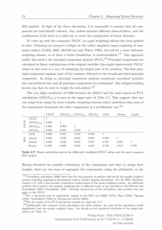
74 Chapter 3. Measuring Ethnic Diversity
fifth quintile. In light of the above discussion, it is reasonable to assume that all com-ponents are individually relevant, they indeed measure different characteristics, and thecombination of all three is a valid way to cover the complexities of ethnic diversity.
To come up with the composite DELF , an equal weighting scheme has been appliedto date. Following an extensive critique on the rather simplistic equal weighting of com-posite indices (Cahill, 2005; McGillivray and White, 1993), the call for a more elaborateweighting scheme, or at least a better foundation, is understandable.177 One approachwidely discussed is the principal component analysis (PCA).178 Principal components arecalculated as linear combinations of the original variables (the single characteristic DELF
values in this case) in a way of explaining the largest part of its variation. The first prin-cipal component explains most of the variance, followed by the second and third principalcomponent. In doing so, principal component analysis transforms correlated variablesinto uncorrelated ones and all principal components are orthogonal. The assigned loadingfactors can then be used to weight the sub-indices.179
The very high correlation of 0.999 between the DELF and the index based on PCAcalculations (DELFP CA) is seen in the upper part of Table 3.7. This suggests that onecan resign from using the more complex weighting schemes and it underlines that none ofthe components dominates the other components in a problematic way.180
DELF DELFP CA DELFGeo DELFP c ANM Alesina Annett
DE
LF
DELF 1DELFP CA 0.999 1DELFGeo 0.963 0.963 1DELFP c 0.994 0.994 0.959 1
ELF
ANM 0.698 0.697 0.707 0.736 1Alesina 0.628 0.630 0.632 0.662 0.800 1Annett 0.630 0.630 0.651 0.671 0.874 0.883 1Fearon 0.607 0.606 0.626 0.621 0.748 0.817 0.795
Table 3.7: Rank correlation matrix for differently weighted DELF values and the most commonELF indices
Having discussed the possible redundancy of the components and ways to assign theirweights, there are two ways to aggregate the components; using the arithmetic, or the
177Chowdhury and Squire (2006) show that the vast majority of scholars still opt for the equally weightedaverage regarding aggregated development indices, despite ongoing discussions. For the HDI, Nguefack-Tsague et al. (2011) also provide a statistical reinforcement of the equal weighting scheme. An additionalproblem often raised is the implicit weighting due to different scales of the sub-indices (McGillivray andNoorbakhsh, 2004; Noorbakhsh, 1998). Through construction of the sub-indices, this problem does notapply to the DELF .
178For a discussion and its application, mainly to the HDI, see Jolliffe (1973), Ram (1982), Ogwang(1994), Noorbakhsh (1998) or Ogwang and Abdou (2003).
179For the results of the PCA and further details, see Appendix C.2.180Additionally, the variances of the sub-indices are rather similar. So, none of the sub-indices wouldsignificantly bias the equally weighted index. For details on key statistical attributes of the single sub-indices, see Table 3.8.
Philipp Kolo - 978-3-653-02395-4Downloaded from PubFactory at 01/11/2019 11:11:06AM
via free access

Chapter 3. Measuring Ethnic Diversity 75
geometric mean.181 Using a geometric mean does ‘penalize’ high dissimilarity in one ofthe components, however. This is often used in composite indices on various inequalitymeasures, e.g., poverty, where the direct compensation of one component through anotheris not desired.182 Two individuals from the same ethno-racial and language backgrounds,who adhere to different religions, would be completely different in the case of a geometricmean because the religious component would be zero.183 That a certain similarity stillprevails between both individuals/groups is obvious. Thus, for the application here, aform of compensation between components seems reasonable. In connection with thediscussion above, the interpretation of the cumulative nature of the characteristics is moreperspicuous and, additionally, argues in favor of an arithmetic mean. Due to these verydifferent attributes, it is not surprising that the DELFGeo has a lower, yet still very highcorrelation to all the other DELF values.
As an alternative, the introduction of a certain non-linearity of compensation betweencharacteristics might be reasonable. This is, for example, promoted by Branisa et al.(2009). To allow for a certain compensation, one squares the components before thecalculation of the arithmetic mean. This leads to an adjusted value of DELFP c. In linewith Nardo et al. (2005), in this approach the weights are interpreted as trade-offs andnot as importance coefficients.184
Finally, the DELF index should contain different information than other indices thattry to measure ethnic fragmentation or diversity. Thus, the redundancy considerationsregarding the components can be applied as a comparison to existing ELF indices. Theresults are found in the lower part of Table 3.7. All rank correlations between the mostcommon ELF indices and the new DELF fall below both redundancy thresholds.185 Al-though already alluded to the theoretical discussion, where it was apparent that bothindices measure different things (fragmentation versus diversity), the statistical resultsprovide additional confirmation.
181An additional aggregation for the DELFP CA index is not necessary because, by construction, thedistance vector of the first principal components contains the weights and aggregation implicitly.
182The HDI just recently switched from an arithmetic mean to a geometric one. To advance a country’sdevelopment it now needs to advance much more equally across the sub-indices than before, where onecould compensate for one index with another. A geometric mean for an index would also imply a clearassignment of both a bad and good state for the values of zero and one. This is possible for povertyand development indices but not for the DELF , which describes a state between two extremes withoutvaluation.
183Collier and Hoeffler (2002), Collier and Hoeffler (2004) and Collier et al. (2004) use a multiplicativecombination of the ethnic and religious fractionalization measure to assess ‘social fractionalization’. Toavoid the dominance of one characteristic, where two groups are completely different, they add the indexwhich is the greater to the product of both indices.
184Thus, an individual can reduce the distance between another individual that does not adhere to thesame religion by learning his language. For further theoretical discussions on weighting and differencesbetween compensatory and non-compensatory approaches, see Munda and Nardo (2005). Branisa et al.(2009) offer a functional operationalization.
185Note that the number of observations varies across the correlation values with the ELF indices due totheir more limited observations.
Philipp Kolo - 978-3-653-02395-4Downloaded from PubFactory at 01/11/2019 11:11:06AM
via free access

76 Chapter 3. Measuring Ethnic Diversity
The arithmetical average between the single characteristics is therefore the easiest wayto operationalize the composite DELF index. Furthermore, it has the compensatoryattributes between the characteristics that reflects their complementarity. This is notgiven by using the geometric mean, for example. By using the part compensation methodand principal components, comparably adequate results are found to those of the simplearithmetic mean. As their correlation is rather high, the method used here follows theprinciple of keeping it as simple as possible.186
3.6 Results
For each country, a similarity matrix is calculated, containing all skl for the weighting ofmutual group similarities. Tables C.2 and C.3 of Appendix C.2 detail the general similaritymatrix calculation. The group similarity calculations are comparable to the ones within acountry and for the difference between countries.
3.6.1 Diversity measure within countries
The size of the respective K × K matrices for each country is defined by the number ofgroups found in it, ranging from 3 to 884.
0.2
.4.6
.81
DE
LF v
alue
s
0 .2 .4 .6 .8 1ELF values
DELF − Composite
0.2
.4.6
.81
DE
LF v
alue
s
0 .2 .4 .6 .8 1ELF values
DELF − Language
0.2
.4.6
.81
DE
LF v
alue
s
0 .2 .4 .6 .8 1ELF values
DELF − Ethno−racial
0.2
.4.6
.81
DE
LF v
alue
s
0 .2 .4 .6 .8 1ELF values
DELF − Religion
Figure 3.2: Combined and single characteristic DELF values against ELF values.
186For further details on all weighting schemes, see Appendix C.2. A detailed discussion of the superiorityof the equal weighting scheme is found in McGillivray and Noorbakhsh (2004), who conclude that moreelaborate weighting schemes ‘‘produce values which are generally indistinguishable from values of theequally weights index’’ (McGillivray and Noorbakhsh, 2004, p. 15). Comparably, de Groot (2009) uses thesame approach in his ethno-linguistic affinity index.
Philipp Kolo - 978-3-653-02395-4Downloaded from PubFactory at 01/11/2019 11:11:06AM
via free access

Chapter 3. Measuring Ethnic Diversity 77
To make the differences between the ELF and DELF values clear, Figure 3.2 showsthe influence of the various characteristics.187 By adjusting for the language differencesonly, reduces the values by less than when all three characteristics are considered. Themost influential changes emerge if religion is taken into account, since in many countries amajority religion is present, which acts as a unifying characteristic. The combined DELF ,weighting all three characteristics, yields more consistent values, which is confirmed inTable 3.8. The standard deviation of the composite DELF is considerably lower thanthose of the decomposed indices.
Religious and language homogeneity, in particular, are spread differently across regions.This is why the adjustments also vary significantly between regions. In Latin-America,188
Spanish is the dominant language, although there are different ethno-racial and/or religiousgroups. The language similarities add to a higher affinity between the groups and, in turn,lower the DELF values. Table 3.9 summarizes the mean values for different ELF andDELF specifications across regions. Additionally, it compares the average ranks of thecountries in the respective groups. A rank of one is assigned to the most heterogeneouscountries, i.e., the countries with the highest ELF or DELF values. Comparing bothranks gives a good indication of how large the adjustments in the DELF calculation arecompared to the standard ELF values.
Index Observations Mean Std. Dev. Min. Max.ELF 210 0.563 0.270 0.019 0.982DELF 210 0.252 0.157 0.006 0.636DELFL 210 0.353 0.243 0.008 0.942DELFE 210 0.255 0.176 0.002 0.708DELFR 210 0.148 0.188 0.000 0.648
Table 3.8: Main statistical characteristics of DELF values, decomposed for all ethnicity charac-teristics
Sub-Saharan Africa (SSA) demonstrates a much higher value when measured by the ELFcompared to the DELF , resulting in a negative rank delta. As seen earlier, this re-gion includes countries with the highest number of groups, mirrored by high ELF values.However, if one takes the similarity between the groups into account, the ranks decrease.Eastern Europe, in contrast, shows much more diversity when considering the DELF valuerather than the ELF value.
More interesting is the decomposition of the DELF into its single characteristics. Forthe language characteristic, Latin America hosts the most homogeneous countries, whereasSub-Saharan Africa again shows the most heterogeneous ones. Taking into account onlythe ethno-racial aspect, Latin America shows the highest diversity. This might come fromthe interbreeding of the native Indian population with the high number of descendantsfrom the Western colonial powers and the resulting Mestizo progeny. The region with
187Both indices are based on WCE data.188Includes the Caribbean.
Philipp Kolo - 978-3-653-02395-4Downloaded from PubFactory at 01/11/2019 11:11:06AM
via free access

78 Chapter 3. Measuring Ethnic Diversity
the most homogeneous countries in this regard is Eastern Europe, a region where outsidepowers have interfered less. The religious characteristic again demonstrates the expecteddistribution. Sub-Saharan Africa has the most religiously heterogeneous countries andWestern and Latin American countries, with high numbers of Christians, host the mosthomogeneous ones. Not surprisingly, the Middle East and Northern African (MENA)countries also show values indicating rather homogeneous religious characteristics, whichis not surprising considering the high proportion of Muslims in these areas. Most countriesthat have a majority religion, i.e., more than 60% of the population either adhere toChristianity (133 countries) or to Islam (43 countries), exhibit rather low religious DELF
values. For all other countries, where there is either no majority religion or it is madeup of another denomination, show significantly higher religious DELF values. Also, theiraverage overall DELF rank is substantially higher than when only taking the number ofgroups in the ELF value into account.
Mean valuesObs. ELF DELF DELFL DELFE DELFR Rank
ELFRankDELF
DeltaRank
Asia 40 0.608 0.290 0.435 0.240 0.194 93.3 90.8 2.5E. Europe 29 0.389 0.197 0.261 0.204 0.126 145.9 125.0 20.8L. America 38 0.509 0.227 0.220 0.386 0.075 121.3 114.5 6.8MENA 21 0.558 0.249 0.358 0.275 0.114 108.1 107.0 1.2SSA 49 0.741 0.319 0.490 0.219 0.248 62.6 81.2 -18.6W. Count. 33 0.465 0.184 0.279 0.206 0.066 128.7 130.9 -2.2World 210 0.563 0.252 0.353 0.255 0.148 – – –Muslim 43 0.571 0.262 0.389 0.271 0.127 105.6 100.7 4.9Christian 133 0.519 0.208 0.299 0.251 0.076 115.7 121.2 -5.7Other 34 0.729 0.407 0.519 0.249 0.454 65.6 50.1 15.5
Table 3.9: Mean ELF and DELF values and ranks for all regions and countries with mainmajority religions
The single country perspective shows even more considerable adjustments. The ELF andDELF values of each country are listed in Table C.7 of Appendix C.3. The countries areordered according to their ELF values in descending order, from the most heterogeneouscountry to the most homogeneous country. The third column depicts their correspondingDELF values and DELF ranks. The difference between the ELF and DELF ranks isshown in column four. The next column outlines the DELF values, decomposed for eachcharacteristic, which helps to better illustrate the adjustments.189 An adjustment of over40 places is seen by half of the 10 most diverse countries. Looking at the lower end, one seesonly marginal adjustments, as expected. The 15 most homogeneous countries are, withthree exceptions, the same for both indices. For the other countries, however, significantadjustments are found. For example, Zambia, the Republic of Congo, Zimbabwe, Angola
189From Figure C.7 of Appendix C.1.3, one can see that the adjustments will tend to be more significantfor higher values of ELF than for lower ones, where both indices are much closer. This is clearly visiblefor the higher ELF values at the top of Table C.7.
Philipp Kolo - 978-3-653-02395-4Downloaded from PubFactory at 01/11/2019 11:11:06AM
via free access

Chapter 3. Measuring Ethnic Diversity 79
and Italy, which are treated as much more homogeneous by the DELF compared to theELF, show difference in ranking of more than 100 places are. Nevertheless, one also findsadjustments in the opposite direction, i.e., countries that have a higher diversity rank basedon DELF values. The countries with the most significant adjustments in this regard – allmore than sixty places – are Kazakhstan, Bahrain, Macedonia, Lebanon, Sudan and theRussian Federation. These upward changes are mainly driven by relatively high languagediversity.
3.6.2 Similarity measure between countries
To date, most authors have focused on the assessment of ethnicity within a country, ashas this essay. This has also been the case in analyzing a country’s growth or conflictincidence. De Groot (2009) expands upon this and proposes his index of ethno-linguisticaffinity (ELA) to measure the similarities between two neighboring countries. He showsthat conflict spillovers are more likely between contiguous countries sharing stronger ethnicsimilarities. The extended calculation for the DELF between countries is nearly identicalto Equation 3.7, and is defined through:
DELFij = 1−K∑
k=1
M∑m=1
pik pjm skm (3.10)
where country i hosts groups k = 1, ...,K, and country j groups m= 1, ...,M , respectively.The distance between the two groups k and m is given through skm. The result is theexpected dissimilarity between two individuals randomly drawn from each country.
The 210 countries analyzed here give a matrix containing over 150 million similarityvalues and nearly 44,000 dyadic relations between countries.190 Due to the amount ofcountry-pairs, only a discussion of averages and some tuples with the highest discrepancyis offered here.191 Naturally, all DELF values are much higher than those for individualcountries. Table C.8 of Appendix C.3 lists the mutually most similar and dissimilar coun-tries at the single country level.192 Many of the mutually most similar countries come fromthe MENA region. The religious homogeneity of this region plays an important role intheir overall similarity level. It is not surprising that the most dissimilar pairs are matchesbetween Asian and African countries. Except for some minority migrant groups, one does
190This significantly exceeds the 2,809 dyadic relations offered by de Groot (2009) for the 53 Africancountries.
191The complete data set can be received upon request.192In general the interpretation of the DELF value between countries ranging between zero and one iscomparable to the case of DELF values within countries. Two countries that consist of groups that sharenot a single characteristic show a mutual DELF value of one, being completly different. Lower values ofDELF correctly indicate countries that share more characteristics and thus are more ‘similar’. However,the theoretical country setup maximizing the similarity between two countries (minimizing the DELFvalue) deviates in its limit from the generally understood meaning of the word ’similar’. This is discussedin more detail in Appendix C.2.6. I would like to thank Walter Zucchini for this important comment.
Philipp Kolo - 978-3-653-02395-4Downloaded from PubFactory at 01/11/2019 11:11:06AM
via free access

80 Chapter 3. Measuring Ethnic Diversity
not find many shared ethnic characteristics between these countries and all their valuesare close to one.
A regional aggregation also offers come interesting insights. For the calculation ofthe regional averages, the DELF values between countries are adjusted for the differentpopulation sizes of the respective country pairs.193 Table 3.10 summarizes the regionaland global averages.
Regional DELF Country pairsAsia 0.719 1,600Eastern Europe 0.479 841Latin America 0.340 1,444North Africa & Middle East 0.430 441Sub-Saharan Africa 0.643 2,401Western Countries 0.572 1,089World 0.841 44,100
Table 3.10: DELF average by main geographical regions
The global cultural diversity measured by the DELF displays an average of 0.84. Asiaexhibits the highest diversity level compared to all other regions. Thus, from a regionalperspective, Asia seems to be the most diverse region, and not SSA.194 Latin America, incontrast, displays the least interregional diversity.
The regional level of diversity plays an important role in the European Union (EU). Thesuccess of European integration is often questioned by the high level of cultural diversity.This was debated before the last enlargement in particular, when the EU grew from 15 to25 and shortly after to 27 member states. It will eventually lead to even more controversialdebates regarding future enlargement plans. With the above approach, the developmentsin the level of diversity through language, ethno-racial, and religious characteristics, caneasily be traced.
Figure 3.3 shows the diversity level of the EU for each wave of enlargement.195 Thepredecessor of today’s EU was initiated in 1952, including Belgium, France, Germany,Italy, Luxembourg and the Netherlands. This ‘core Europe’, which it is often referredto, displayed a regional DELF value of 0.37. The next two enlargement waves addednearly 25% to the total population. However, these countries were not overly differentfrom the existing group and were internally rather homogeneous. Hence, the DELF onlyslightly increased. The addition of Portugal and Spain in 1986, two populous and veryhomogeneous countries, slightly decreased the overall level of European diversity, whereas
193For the weighting, population data averages for 2005–2010 from the World Development IndicatorsWorld Bank (2011) were used. For more details on how regional averages are calculated and the differencesin the calculation of DELF values between countries, see Appendix C.2.7.
194Note that from the single country perspective, SSA still has the countries with the highest internalheterogeneity. This is an indication that the drawing up of borders in Asia proceeded more ‘endogenously’than the method used in SSA by the colonial powers.
195For more details on the different waves of enlargement in the EU, and the respective diversity levels,see Table C.9 of Appendix C.3.
Philipp Kolo - 978-3-653-02395-4Downloaded from PubFactory at 01/11/2019 11:11:06AM
via free access

Chapter 3. Measuring Ethnic Diversity 81
Figure 3.3: Average DELF values of the EU per enlargement wave
the huge enlargement of 10 countries in 2004, and of two more in 2007, again increasedthe DELF level significantly.196 Looking at potential future enlargements, the admissionof mainly Balkan states, as well as Iceland (EU+B), would not change the status quogreatly. The highest increase in diversity within the EU would result from admittingTurkey (EU+T). The increased cultural diversity Turkey would bring to the EU can’tbe judged as good or bad, per se – however, it offers an easy target for exploitation ofthese differences and political agitation. This was already the case during earlier waves ofenlargement which only displayed marginal increases in the EU’s diversity. The increaseTurkey would bring, as stated, would be far greater, thus the potential for exploitationand political agitation could be far greater.
Finally, the DELF values between countries are compared with the most widely usedmeasure of cultural distance between countries, its genetic distance. By matching thesewith the detailed data on genetic diversity compiled by Spolaore and Wacziarg (2009),yields only a very limited correlation (Table 3.11).197 The rank correlation of genetic dis-tance and the composite DELF is only 0.25, and thus fail to meet both of the redundancythresholds discussed above.198 This comparison underlines that the genetic distance datais hardly a good proxy for the ‘cultural’ differences between countries.
196One important caveat applies for this. As essay 2 outlined, cultural heterogeneity levels are subjectto change. As the underlying data for the DELF calculation is dated for the years 2005–2010, using itfor time frames of over 50 years ago will lead to distorted values. Thus, the DELF values for the EUenlargement for the earlier years can only be taken as an indication. The changing DELF values are onlyattributable to compositional changes of the European Union and not to expectable changes over time.
197Spolaore and Wacziarg (2009) construct two measures of genetic relatedness between countries. Oneis based only on the genetic distances between the plurality ethnic groups of each country. The second isa measure of weighted genetic distance of all groups. The latter construction is more comparable to theone employed in this essay.
198As expected from the characteristic definition, the highest correlation of the genetic data is with theethno-racial DELF values at 0.7. Both are correlated but still seem to measure different things.
Philipp Kolo - 978-3-653-02395-4Downloaded from PubFactory at 01/11/2019 11:11:06AM
via free access
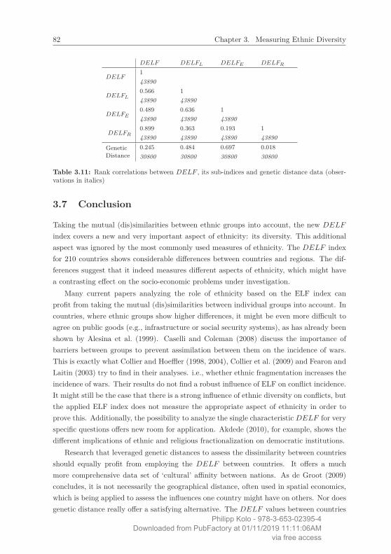
82 Chapter 3. Measuring Ethnic Diversity
DELF DELFL DELFE DELFR
DELF143890
DELFL0.566 143890 43890
DELFE0.489 0.636 143890 43890 43890
DELFR0.899 0.363 0.193 143890 43890 43890 43890
GeneticDistance
0.245 0.484 0.697 0.01830800 30800 30800 30800
Table 3.11: Rank correlations between DELF , its sub-indices and genetic distance data (obser-vations in italics)
3.7 Conclusion
Taking the mutual (dis)similarities between ethnic groups into account, the new DELF
index covers a new and very important aspect of ethnicity: its diversity. This additionalaspect was ignored by the most commonly used measures of ethnicity. The DELF indexfor 210 countries shows considerable differences between countries and regions. The dif-ferences suggest that it indeed measures different aspects of ethnicity, which might havea contrasting effect on the socio-economic problems under investigation.
Many current papers analyzing the role of ethnicity based on the ELF index canprofit from taking the mutual (dis)similarities between individual groups into account. Incountries, where ethnic groups show higher differences, it might be even more difficult toagree on public goods (e.g., infrastructure or social security systems), as has already beenshown by Alesina et al. (1999). Caselli and Coleman (2008) discuss the importance ofbarriers between groups to prevent assimilation between them on the incidence of wars.This is exactly what Collier and Hoeffler (1998, 2004), Collier et al. (2009) and Fearon andLaitin (2003) try to find in their analyses. i.e., whether ethnic fragmentation increases theincidence of wars. Their results do not find a robust influence of ELF on conflict incidence.It might still be the case that there is a strong influence of ethnic diversity on conflicts, butthe applied ELF index does not measure the appropriate aspect of ethnicity in order toprove this. Additionally, the possibility to analyze the single characteristic DELF for veryspecific questions offers new room for application. Akdede (2010), for example, shows thedifferent implications of ethnic and religious fractionalization on democratic institutions.
Research that leveraged genetic distances to assess the dissimilarity between countriesshould equally profit from employing the DELF between countries. It offers a muchmore comprehensive data set of ‘cultural’ affinity between nations. As de Groot (2009)concludes, it is not necessarily the geographical distance, often used in spatial economics,which is being applied to assess the influences one country might have on others. Nor doesgenetic distance really offer a satisfying alternative. The DELF values between countries
Philipp Kolo - 978-3-653-02395-4Downloaded from PubFactory at 01/11/2019 11:11:06AM
via free access

Chapter 3. Measuring Ethnic Diversity 83
offer an excellent and valid extension of the analysis into spillover effects between countries.De Groot (2009) shows the role cultural affinity between neighboring countries plays inthe spillover of conflicts.
Trust is associated closely with more homogeneous and similar country setups. Geneticdistance only covers trust in a very limited way. Trust is seldom hidden in the genetic code,evolving out of the interaction between individuals whose cultural backgrounds play animportant role.199 Leveraging genetic distance is even more problematic in Spolaore andWacziarg’s (2009) analysis on the spillover effect of innovations and development betweencountries. Imitation and adaptation costs of innovations rely significantly more on the‘cultural’ barriers (different language, ethno-racial background and beliefs) than on thebiological ones (genes).
Nevertheless, there are some caveats that one cannot overlook. As the data sourceused is somewhat unique in its combination of all characteristics, only limited robustnesschecks with other sources on the combination of the characteristics are possible. Secondly,the weighting of the three sub-indices is debatable, as is the case for most composite indexcalculations. Here, the most general approach is used. For specific questions, differentemphasis might be given to specific characteristics. The clear discussion and overview ofthe single sub-indices should encourage every researcher to do so. Finally, there mightbe country or region-specific characteristics influencing cultural diversity not covered inthe (globally comparable) three characteristics treated in this essay. The caste system inIndia would be one example. Thus, for a country or region-specific analysis, the diversitydata offered might have restricted relevance. Nevertheless, the approach discussed herecan still be applied.
In the above cases the DELF index should be more appropriate than the ELF indexas it incorporates the fundamental concept of diversity. The extension to measure culturaldissimilarities between nations offers a good alternative to the applied genetic distancedata. The broad foundation and the detailed new data set should be a call to criticallyreview the usage of the ELF index and the genetic distance data. Additionally, it providesa starting point for new research on the specific role of the diversity of countries.
199For an indication of how a common language increases trust and common identification in a case studyfor the US, see Chong et al. (2010). Falck et al. (2010) show that German cross-regional migration andeconomic exchange can be attributed to dialect similarities from the 19th century that remain today.
Philipp Kolo - 978-3-653-02395-4Downloaded from PubFactory at 01/11/2019 11:11:06AM
via free access

Philipp Kolo - 978-3-653-02395-4Downloaded from PubFactory at 01/11/2019 11:11:06AM
via free access

Chapter 4
The Implications of EthnicDiversity
4.1 Introduction
Recent literature on the role of ethnicity in socioeconomic contexts has strived to finddifferent ways of measuring its various aspects. Most papers rely on an index coveringthe fragmentation (ELF) or the polarization (POL) of a country’s ethnic groups.200 Ingeneral, the ELF is an increasing function of the number of groups. A country with more,and thus smaller relative groups, is more fragmented. On the contrary, the POL measuresthe deviation from a situation of two equally sized groups. For such a setup, the POLreaches its maximum value and decreases afterwards. Already from their construction onecan see that both measures cover different ethnic setups and are therefore supposed toexplain different problems. The distance adjusted ethno-linguistic fractionalization indexDELF now adds a third aspect, a country’s ethnic diversity.
For many economic problems, it is not the pure quantity of (relative) groups which isof interest, but the difficulty of coordination or instrumentalization between them. Thisis crucially dependent on the differences between these groups and not only on their mereexistence. Thus, one expects the DELF to exhibit a different performance on a range ofeconomic questions compared to the ELF and POL. This chapter shows the applicabilityof the DELF index in different fields, selected as to cover a broad range of economicproblems.201
The mere quantity of groups might demonstrate more divisions through which conflictsmay ignite, arguing for the ELF index. To the contrary, in very heterogeneous countries,
200See, for example, Mauro (1995), Easterly and Levine (1997), Collier (2001), Alesina et al. (2003) andAlesina and La Ferrara (2005) for different applications of the ELF concept and Duclos et al. (2004),Garcia-Montalvo and Reynal-Querol (2002, 2005b, 2010) and Ranis (2011) for the application of the POLindex.
201Additionally, limited access to the underlying data of some relevant articles in the respective fields hin-dered a broader testing of the applicability of the index, therefore affecting the selection of the replications.Again, a sincere thank you to all authors who generously shared their data for this study.
Philipp Kolo - 978-3-653-02395-4Downloaded from PubFactory at 01/11/2019 11:11:06AM
via free access
86 Chapter 4. The Implications of Ethnic Diversity
with many small groups, coalition building to create a strong enough power base becomesmore difficult. This is why others argue that it is the specific quantitative constellationof groups, i.e., their polarization (POL), that impacts the incidence of conflicts (Garcia-Montalvo and Reynal-Querol, 2005b). Caselli and Coleman (2008) point to obvious barri-ers between groups that are important regarding the decision to enter conflicts. If a groupcan easily exclude another (potentially the defeated group) from the resources gained (dueto an obvious ethnic identifier existing between both groups), it raises the incentives tostart a conflict. This would argue for an important role of the diversity measure DELF .Thus, it is difficult to decide a priori which ethnicity index better explains conflicts.
A high ethnic fragmentation is associated with lower growth rates, mainly through itseffect on other socioeconomic variables (e.g., corruption or public goods provision).202 Themore groups that exist, the more visions regarding the realization of education, locationand forms of infrastructure, or the design and extent of institutions, differ. Because everygroups wants at least some of its wishes to be met, the government’s difficulty in achievinga consensus, and the distribution of its available funds might indeed depend on the merequantity of groups, reflected in a higher fragmentation (ELF). In contrast, the differentbackgrounds and experiences of a country’s working population may be an asset to sustainmore complementary production procedures and drive innovation. For this, not only themere quantity of groups, but also their differences seem to be relevant. This potentialmight, however, only unfold in more developed countries.203 Whether, and how the ELFor the DELF may impact on economic growth is, again, not completely clear.
Trust is an important precondition for nearly any transaction. Different groups shouldequally influence the general trust level in a country. Bjørnskov (2008), however, finds nosignificant impact of fractionalization (ELF) on trust. This might be true due to the factthat the quantity of groups in a country are less relevant to the emergence of trust, thanthe differences between them (which only the DELF takes into account). Unfortunatelythis can’t be confirmed by the following analyses.
The DELF has an additional huge advantage, in that it can be used to assess thecultural differences between countries. For both the ELF and POL, this is not possible.Thus far, bilateral differences between cultures were assessed by data based on quitelimited differences (e.g., genetic distance) or a broad set of proxy variables that are oftenregionally bounded (e.g., mutual voting behavior at regional song contests). The globalDELF data shall offer some escape from these limitations. Again, taking the level of trustas an important prerequisite for any economic activity, cultural diversity affects the levelof positive opinions between countries (Disdier and Mayer, 2007). More specifically, the
202The most prominent are Easterly and Levine (1997), Alesina et al. (2003) and Alesina and La Ferrara(2005).
203One can, however, also argue that with a rising difference between the groups a consensus becomeseven more difficult and thus a high diversity should also have a negative impact on growth. For thesepotentially different effects, the development level of a country seems to be especially crucial and will befurther discussed in section 4.4.
Philipp Kolo - 978-3-653-02395-4Downloaded from PubFactory at 01/11/2019 11:11:06AM
via free access

Chapter 4. The Implications of Ethnic Diversity 87
DELF shows a significant impact on trade volumes in two analyses with an Europeanfocus. It substitutes a list of various cultural affinity proxies very well, thus paving theway to expand these trade analyses on to a global scale.
The remainder of this chapter is organized as follows. Section 4.2 gives a short overviewof the main indices commonly used and outlines the clear distinction between them andthe DELF index. In section 4.3, the DELF is tested based on its implications for conflictincidence. The differing impact of ethnic diversity on economic growth is analyzed insection 4.4. Section 4.5 discusses the potential improvements of the diversity measureagainst the fractionalization measure for the level of trust within and between countries.Section 4.6 again uses DELF values between countries to identify its role on bilateraltrade. Finally, section 4.7 summarizes the key findings, concludes, and gives an outlookfor further research.
4.2 Overview of relevant indices
The most commonly used index to cover ethnicity in the economic context is the ethno-linguistic fractionalization index (ELF). It was first published for a broad range of countriesby Taylor and Hudson (1972).204 The ELF is calculated as an Herfindahl-Hirschmanconcentration index:
ELF = 1−K∑
i=1p2
i , for all i ∈ {1, ...,K} (4.1)
where K is the number of groups i, and pi represents their relative group sizes. Its valuemoves between zero and one and represents the probability that two randomly selectedindividuals from a population come from different groups. A higher value indicates a morefragmented country, i.e., a country with a higher number of distinct ethnic groups.
The second prominent measure is an index of polarization, introduced by Garcia-Montalvo and Reynal-Querol (2002).205 Assessing the variation outside of an even 50/50split of two groups, Garcia-Montalvo and Reynal-Querol (2002) find that this index isa much better predictor for conflict incidence than the ELF measure. The polarizationindex (POL) is defined as:
POL = 1−K∑
i=1
(0.5−pi
0.5
)2·pi, for all i ∈ {1, ...,K} (4.2)
The POL index also tends towards zero for very homogeneous countries, i.e., with onlyone group. However, with increasing group numbers, ELF and POL show clearly different
204Ginsburgh and Weber (2011, Ch. 6) offer a good overview of the different classes of indices used, theirhistorical development and recent applications. For a broad overview on general concepts and measures ofethnicity, see Brown and Langer (2010).
205Their work is considerably based on Esteban and Ray (1994).Philipp Kolo - 978-3-653-02395-4
Downloaded from PubFactory at 01/11/2019 11:11:06AMvia free access

88 Chapter 4. The Implications of Ethnic Diversity
courses. While ELF is an increasing function of the number of groups, POL reaches itsmaximum with two equally sized groups and decreases afterwards.
The DELF now takes the distance between these groups into account. The idea datesback to Greenberg (1956), and later Fearon (2003), who both proposed using linguisticsimilarities between language groups to cover the distance aspect. In addition to thelanguage characteristic, the DELF includes information on the ethno-racial and religiouscharacteristics of all groups.206 The three characteristics are weighted to arrive at thecomposite DELF values.207 Aligned with the ELF index, the DELF index is calculatedas:
DELF = 1−K∑
k=1
K∑l=1
pk pl skl, for all k, l ∈ {1, ...,K} (4.3)
where the combined skl is the equally weighted average of the similarity values of eachethnicity characteristic between all groups k, l ∈ {1, ...,K}. This new global data set isbased on data from the World Christian Encyclopedia (Barrett et al., 2001) and offersethnic diversity data for 210 countries. By construction, a close relationship to the ELFmeasure is evident. Both are influenced by the number of groups, which in a way determinethe relative groups sizes – a key building block for both. Based on this additional aspect,accounting for the differences between groups, the DELF leads to significant differencesbetween a country’s ELF and its DELF values. Figure 4.1 shows the ranks of all countriesdepending on its ELF and DELF values, where the highest values correspond with therank of one.208 Changes in the heterogeneity ranking of more than 30 places (indicatedby the dotted lines) are quite common. Countries such as Zambia, the Republic of Congo,and Zimbabwe seem to be more homogeneous when using the DELF compared to theirELF values. Contrarily, Kazakhstan, Bahrain or the Sudan turn out to be more diversethan fragmented.
In addition to the diversity data of single countries, the index offers information onnearly 44,000 dyadic relations between countries and their respective cultural distance.This is a key advantage of the DELF as the ELF and POL do not allow for any assessmentof ethnic differences between countries. For this reason, an index of genetic distance wasoften used, although one may raise some reasonable objection to its applicability.209 It isbased on a rather limited number of 42 distinct world populations for its calculation and
206Two other recent approaches consider a set of characteristics to assess the differences between groups.Bossert et al. (2011) combine ethnic and various socioeconomic differences between citizens to constructELF values comprising of diversity for US counties. De Groot (2009) measures a broad set of culturalcharacteristics (e.g., language, religion) to assess the ethno-linguistic affinity between countries in Africa.
207For more details on the distance calculations for each characteristic and the different weighting possi-bilities, see the Appendix C.2.
208More details on the ELF and DELF values are found in Table C.7 of Appendix C.3.209The assessment of genetic distance can be traced back to the pioneering work of Cavalli-Sforza andFeldmann (1981), who created phylographic trees by mapping the differences in special sections of thehuman DNA.
Philipp Kolo - 978-3-653-02395-4Downloaded from PubFactory at 01/11/2019 11:11:06AM
via free access

Chapter 4. The Implications of Ethnic Diversity 89
Figure 4.1: Scatter plot of ELF and DELF rank values
turns out to be a predictor for geographic distance from a common place within Africa(Giuliano et al., 2006; Ramachandran et al., 2005). The global DELF values betweencountries offer a good option to escape from these limitations.
4.3 Implications of ethnic diversity on conflict
The relationship between ethnic division and conflict is probably the most researched fieldregarding a possible impact of ethnicity. Due to this, different aspects of conflict have beenhighlighted. The analyses of its roots and influencing factors differ for the incidence, onsetand duration of conflicts. While incidence measures if any form of conflict is currentlyoccurring in a given country, its onset measures whether a specific conflict starts at agiven time. For example, a country that experiences a two year conflict, exhibits a conflictincidence for both years, but conflict onset only in the first year. Finally, the durationmeasures the overall length of a given conflict. In the aforementioned example, this wouldbe two years.210
For conflicts in general, greed, rather than grievance is held responsible (Collier andHoeffler, 2004). More opportunities to hide in mountainous regions, the possibility of gain-ing higher amounts of natural resources, and lower opportunity costs for an impoverishedpopulation are brought forward as arguments. However, the more ethnic groups that areoppressed by the ruling regime raises the probability of revolts. Not only oppression, butmarginalization and the intentional underdevelopment of groups not belonging to the rul-ing clan may raise tensions, which may develop into conflicts. In line with the greed andopportunity theories, a broad strand of literature relying on the ELF index has not found
210For more details on the different conflict measures, see Bleaney and Dimico (2009).Philipp Kolo - 978-3-653-02395-4
Downloaded from PubFactory at 01/11/2019 11:11:06AMvia free access

90 Chapter 4. The Implications of Ethnic Diversity
strong empirical evidence for a relationship between ethnic fragmentation and any of theconflict measures (Fearon and Laitin, 2003).211 Apparently the mere number of groups isnot that relevant for conflict.212
These arguments led Garcia-Montalvo and Reynal-Querol (2002) to develop a polar-ization index (POL) as a more relevant measure of relationship between ethnic divisionand conflict.213 They argue that deviation from the situation of two equally strong groups,that might both seize power over the whole country, is more relevant for the incidence ofconflicts than the fractionalization of a country. In general, polarization is indeed morerobustly associated with the conflict measures.
In a theoretical contribution, Caselli and Coleman (2008) stress the importance ofpotential excludability of the defeated party from economic or political gains. The possi-bility to exclude another group based on obvious barriers (physiognomic, language, ethnic)between them, raises the incentives to start a conflict. The distance between groups, mir-rored in the DELF index, should be a relevant factor for the consideration of whether ornot to start a war.
Garcia-Montalvo and Reynal-Querol (2005b) test the applicability of ethnic and reli-gious polarization against the respective fractionalization indices in the incidence of wars.They use data from the Peace Research Institute of Oslo (PRIO), which include intermedi-ate and high-intensity armed conflicts. A range of standard control variables (GDP/capita,Population, Primary exports, Mountains, Contingency, and Democracy) are included inall regressions. The regressions in Table 4.1 are replications from the ones in the originalarticle and use a logit model for the incidence of civil wars based on five-year periods.The ethnic polarization variable (Ethnic pol.) clearly outperforms the fractionalizationvariable (Ethnic frac.) in regards to the level of significance.214 All control variables carrythe expected sign.
The regressions in Table 4.2 now rebuild the approach of Garcia-Montalvo and Reynal-Querol (2005b). However, the fractionalization indices are replaced by the compositeDELF and the DELFR.215 The higher significance of the polarization measure (Ethnicpol.) fades and gives way to the composite DELF . The coefficients for the controlvariables and their significances remain more or less unchanged. It is apparent that theDELF , covering the differences between groups, contains important information regarding
211See also Collier and Hoeffler (2004) and Collier et al. (2009).212Furthermore, the quantity of groups, demonstrating more divisions through which conflicts may arise,may make coalition building in order to create a strong enough power base more difficult. This mayadditionally impede a linear relationship of ELF and conflicts.
213This is based on earlier work of Esteban and Ray (1994). Garcia-Montalvo and Reynal-Querol (2005b,2010) further develop the polarization index and its application. See Blattman and Miguel (2010) for abroad literature overview.
214The ethnic variables are also based on data from the World Christian Encyclopedia (Barrett et al.,2001), whereas the religious measures are mainly built based on data from the L’ Etat des Religions dansle Monde (Clévenot, 1987).
215To be consistent, the fractionalization indices were also taken from the same data source as the DELFis calculated, i.e., the WCE.
Philipp Kolo - 978-3-653-02395-4Downloaded from PubFactory at 01/11/2019 11:11:06AM
via free access

Chapter 4. The Implications of Ethnic Diversity 91
(1) (2) (3) (4) (5)Conf. Conf. Conf. Conf. Conf.
Ethnic frac. 1.19* 0.18 0.05(1.89) (0.19) (0.05)
Ethnic pol. 2.38*** 2.29** 2.09**(2.97) (2.23) (2.03)
Rel. frac. -4.97* -4.45(-1.65) (-1.39)
Rel. pol. 3.90** 3.29(1.97) (1.59)
Ln (GDP/capita) -0.29 -0.44** -0.42* -0.33 -0.38(-1.27) (-1.99) (-1.79) (-1.13) (-1.33)
Ln (Population) 0.35** 0.41** 0.40** 0.44*** 0.44***(2.18) (2.40) (2.21) (3.01) (2.72)
Primary exp. -0.91 -1.01 -1.07 -0.35 -0.90(-0.52) (-0.54) (-0.57) (-0.21) (-0.48)
Mountains 0.00 -0.00 -0.00 0.00 -0.00(0.49) (-0.25) (-0.19) (0.29) (-0.16)
Non contiguous 0.08 0.30 0.29 0.31 0.48(0.13) (0.49) (0.48) (0.49) (0.79)
Democracy 0.08 0.03 0.03 0.02 -0.03(0.21) (0.09) (0.09) (0.05) (-0.09)
Constant -5.82** -6.23* -6.30** -6.90** -7.47**(-2.06) (-1.93) (-2.01) (-2.26) (-2.32)
Observations 846 846 846 846 846Pseudo R2 0.101 0.122 0.122 0.110 0.134Cluster robust t statistics in parentheses* p < 0.10, ** p < 0.05, *** p < 0.01
Table 4.1: Original logit regression for the incidence of civil wars as found in Garcia-Montalvoand Reynal-Querol (2005b)
the incidence of conflicts. In line with the contribution of Caselli and Coleman (2008),obvious barriers should play a role in this decision. That the composite DELF , coveringall characteristics, has a significant impact compared to the DELF solely based on religion,confirms their theoretical arguments. In most cases, religious identification may not be anobvious enough characteristic to rule out future assimilation.
Having found a significant impact of DELF on the incidence of conflicts does not,however, allow one to infer its applicability onto other conflict measures, namely its onsetand duration. Further research deems necessary to fully understand the dynamics as tohow the different aspects of a country’s ethnic composition affects the different phases ofconflict.
4.4 Implications of ethnic diversity on growth
The second most prominent question of ethnicity’s role is whether, and how it affectseconomic growth. This was the starting point for the seminal paper of Easterly and
Philipp Kolo - 978-3-653-02395-4Downloaded from PubFactory at 01/11/2019 11:11:06AM
via free access

92 Chapter 4. The Implications of Ethnic Diversity
(1) (2) (3) (4) (5)Conf. Conf. Conf. Conf. Conf.
DELF 2.40* 2.55** 4.25**(1.87) (2.05) (2.31)
Ethnic pol. (WCE) 0.45 0.74 0.28(0.39) (0.64) (0.22)
DELFR -9.59 -12.48(-1.38) (-1.53)
Rel. pol. (WCE) 5.98 6.43(1.35) (1.30)
Ln (GDP/capita) -0.35 -0.47* -0.40 -0.42* -0.47(-1.48) (-1.87) (-1.50) (-1.75) (-1.64)
Ln (Population) 0.39*** 0.40** 0.39** 0.42*** 0.45***(2.59) (2.56) (2.54) (2.75) (3.37)
Primary exp. -0.96 -0.27 -1.00 0.07 -0.46(-0.48) (-0.16) (-0.50) (0.04) (-0.26)
Mountains 0.00 0.00 0.00 0.00 0.00(0.54) (0.30) (0.41) (0.34) (0.17)
Non contiguous 0.10 0.12 0.21 0.05 0.13(0.16) (0.18) (0.31) (0.08) (0.18)
Democracy 0.03 0.08 0.02 0.06 -0.02(0.09) (0.22) (0.05) (0.16) (-0.07)
Constant -6.17** -4.94* -6.10** -5.58* -6.52**(-2.15) (-1.70) (-2.09) (-1.92) (-2.35)
Observations 833 833 833 833 833Pseudo R2 0.108 0.092 0.110 0.101 0.128Cluster robust t statistics in parentheses* p < 0.10, ** p < 0.05, *** p < 0.01
Table 4.2: Logit regression for the incidence of civil wars, based on Garcia-Montalvo and Reynal-Querol (2005b)
Levine (1997), who concluded that Africa’s lower growth rate can be explained to a largeextent by its higher ethnic fragmentation. Their approach was extended and updatedwith new ELF data by Alesina et al. (2003). Subsequently, Schüler and Weisbrod (2010)added an additional decade of observation and thus based their analysis on a broaderfoundation.216 They all very much confirm the negative effect of the ELF on a country’sgrowth rate. For more developed countries with better education and infrastructure, thiseffect is found to be less detrimental (Alesina and La Ferrara, 2005). Ethnic diversitymight even be a driver of innovation for these countries and should thus affect growth in apositive way. Nevertheless, cooperation is apparently more difficult in more heterogeneouscountries so it is natural to question the DELF ’s role in economic growth. As the datacompiled by Schüler and Weisbrod (2010) offers the most observations, it seems obviousto replicate their analyses.
216Whereas Alesina et al. (2003) covered the period from 1960 to 1989, Schüler and Weisbrod (2010)expand the data to cover the period 1960 to 1999.
Philipp Kolo - 978-3-653-02395-4Downloaded from PubFactory at 01/11/2019 11:11:06AM
via free access

Chapter 4. The Implications of Ethnic Diversity 93
(1) (2) (3) (4)Growth Growth Growth Growth
Africa -0.009** -0.014*** -0.012*** -0.016***(-2.66) (-3.47) (-3.67) (-4.27)
La. America -0.016*** -0.014*** -0.018*** -0.016***(-5.93) (-4.63) (-6.60) (-5.08)
Ln (GDP/cap.) 0.041*** 0.027 0.045*** 0.030(2.71) (1.46) (2.89) (1.59)
(Ln (GDP/cap.))2 -0.003*** -0.003** -0.003*** -0.003***(-2.99) (-2.47) (-3.08) (-2.61)
Ln (Schooling) 0.011*** 0.003 0.011*** 0.003(3.40) (0.66) (3.36) (0.66)
Assassinations -21.103** -19.766**(-3.48) (-2.18)
Financial depth 0.009** 0.010**(2.14) (2.00)
Black market premium -0.021*** -0.021***(-5.34) (-5.31)
Fiscal surplus/GDP -0.000** -0.000*(-1.81) (-1.91)
Ln (Telephones/worker) 0.016*** 0.017***(3.15) (3.34)
ELF (Alesina) -0.019*** -0.012**(-3.86) (-2.20)
DELF -0.017** -0.005(-2.34) (-0.58)
Observations 82/88/ 38/67/ 81/87/ 38/67/94/92 74/80 93/91 74/79
R2 0.24/0.24/ 0.46/0.45/ 0.21/0.20/ 0.46/0.44/0.36/0.16 0.49/0.30 0.35/0.12 0.48/0.27
Robust t statistics in parentheses; observation and R2 values are decade specific* p < 0.10, ** p < 0.05, *** p < 0.01Growth is measured as annual growth rate of per capita GDP
Table 4.3: Influence of ethnic diversity on economic growth, based on Schüler and Weisbrod(2010)
Table 4.3 shows, in regressions (1) and (2), replications of the original growth regres-sions of Schüler and Weisbrod (2010).217 Regression (1) contains only limited controlvariables that are supposed to influence the economic development of countries. Bothregional dummies, for Africa and Latin America, are negative and significant at the 5%and 1% levels. The income level (GDP/cap.) at the beginning of each decade shows acatch-up effect, at a slightly diminishing rate as its squared term is negative but witha very small coefficient. As one expects, Schooling has a significant effect on increasing
217The regressions here are run, in line with Schüler and Weisbrod (2010), using seemingly unrelatedregressions (SUR). SUR is used to allow for country random effects to be correlated across decades, inorder to increase the efficiency of the estimators. However, comparing the results to a model run withrobust OLS regressions and decade dummies displays nearly no differences. Thus, the decade correlationsseem to be very limited.
Philipp Kolo - 978-3-653-02395-4Downloaded from PubFactory at 01/11/2019 11:11:06AM
via free access

94 Chapter 4. The Implications of Ethnic Diversity
growth.218 Finally, ethnic fractionalization (ELF), based on the data compiled by Alesinaet al. (2003), reveals a detrimental growth effect. A completely homogeneous countrywould expect an almost 2% higher rate of annual growth compared to a completely frac-tionalized country. The different level of ethnic fractionalization between Korea and Côted’Ivoire is thus responsible for roughly 1.6% of their growth rate differential.219 Regression(2) mow includes a broad set of variables affecting growth. The number of Assassinations,the Black market premium and the Fiscal surplus all negatively affect growth at highlysignificant levels of 1%. Financial depth and the number of Telephones per worker areused as proxies for the level of infrastructure in a country, with both showing a growthenhancing potential and being highly significant. As ethnic fractionalization per se canhardly impact upon growth, all of these variables are meant to be channels through whichethnic fragmentation affects growth. This is supported by a high correlation between theELF and those variables. Indeed, Easterly and Levine (1997) and Alesina et al. (2003)find a vanishing effect of the ELF as the number of covariates included in the regressionsincreases, until it becomes equally insignificant. By including data from the 1990s, Schülerand Weisbrod (2010) find a robust, albeit smaller, negative effect of the ELF on growth,controlling for all other variables. This, therefore, still confirms that the ELF potentiallyworks through affecting these variables.220
Regression (3) now exchanges the ELF values with DELF values. Nearly all of the co-efficients and significance levels remain relatively unchanged and, interestingly, the DELF
displays nearly the same coefficient as the ELF. However, it loses its significant impactwhen all controls are included in regression (4), as in the articles of Easterly and Levine(1997) and Alesina et al. (2003). Although the coefficients look similar their economicimpact differs. Whereas an increase of one standard deviation in the ELF reduces growthby 0.56 percentage points, the same increase in the DELF would only lead to a reductionin growth of 0.29 percentage points.221 Again comparing Korea and Côte d’Ivoire, the dif-ference in their respective DELF levels is responsible for slightly less than one percentagepoint of their growth rate differential.222 Thus, ethnic diversity seems to be less detrimen-tal to economic growth than the ELF. As both affect growth through different variables(channels), a more detailed analysis on ELF and DELF effects is deemed necessary here.
218Measured as the average years of total school attainment at the start of the decade.219In the data of Alesina et al. (2003) Korea has an ELF of 0.002, whereas Côte d’Ivoire has an ELF of0.82.
220If one uses the ELF index based on the same data as the DELF (WCE data), its effect remains highlysignificant in regression (1) but fades again in regression (2).
221The standard deviation of ELF is 0.27, whereas it is only 0.16 for the DELF . For the annual growthrate the standard deviation is 0.027.
222Korea has a DELF of 0.032, whereas Côte d’Ivoire has a DELF of 0.586.Philipp Kolo - 978-3-653-02395-4
Downloaded from PubFactory at 01/11/2019 11:11:06AMvia free access

Chapter 4. The Implications of Ethnic Diversity 95
However, for these basic regressions, the sheer number of groups are more robust thantaking their differences additionally into account.223
Despite the finding that heterogeneity negatively affects economic growth, one canquestion if this relation changes in different country settings. The reasoning for this ispromoted mainly by articles analyzing metropolitan regions and companies.224 They oftenfind that ethnic heterogeneity has a positive effect on innovation and productivity. Withvery comparable data to that above, Alesina and La Ferrara (2005) try to prove thispositive effect in a large scale cross country analysis. They show that the detrimentaleffect of ethnic heterogeneity does indeed fade for more economically developed countries.The original paper, however, relies on the limited dataset from 1960–1989.
Table 4.4 replicates the analysis of Alesina and La Ferrara (2005) with the extendeddata of Schüler and Weisbrod (2010).225 Following the argumentation of Alesina andLa Ferrara (2005) that richer countries are less prone to the ELF’s detrimental effect, theheterogeneity measures (ELF and DELF ) are both interacted with the countries’ incomelevels (GDP/cap.). The negative effects for ELF and DELF remain in regressions (1) and(2), although they are no longer or only marginally significant at conventional levels. Thesame is true for the interaction terms of the heterogeneity measures (ELF/DELF ) andthe level of initial income (GDP/cap.). Thus, the finding of Alesina and La Ferrara (2005)cannot be confirmed for the extended time period. However, it is questionable whether amere higher income level is the basis for diversity to deliver benefits to a country. Countriesneed instead to establish a common base that allows the different groups to interact ina productive way.226 An indicator reflecting a broader perspective of development is theHuman Development Indicator (HDI). Regression (3) and (4) include the HDI level and aninteraction term with the heterogeneity indices, replacing the income level used before.227
The ELF and DELF again enter the regression with the familiar significant negativeeffect, although the DELF is slightly less significant. More interestingly, the interaction
223The static nature of both the ELF and the DELF calls for an important caveat. Chapter 2 showedthat the level of ethnic heterogeneity in a country is changing and makes inter alia education responsiblefor this. Although the ethnic setup of a country does not change quickly, an analysis covering four decades,with a single static ethnic measure, requires some caution.
224Ottaviano and Peri (2005) show that native US citizens receive higher wages in metropolitan areaswhere ethnic heterogeneity is increasing. Again for the US, Sparber (2010) confirms a productivity in-creasing effect of racial diversity for cities, but less so at the state level. Florida (2004) argues that a morediverse agglomeration of creative capital increases innovations and ultimately economic growth. Equally,Niebuhr (2010) finds that cultural diversity raises innovative activity, positively affecting the performanceof regional research and development (R&D) sectors in Germany. Ozgen et al. (2011a) show a comparableresult for European regions. Watson et al. (1993) show empirically that more diverse teams need longerto establish a common understanding, but if that is reached they outperform more homogeneous groups.Similarly, Prat (2002) shows, in a game theoretical analysis, that the positive impact of a heterogeneousversus a homogeneous team depends on the complementarity of their tasks. A comparable result is alsofound in Hong and Page (1998).
225The regressions are again run with robust OLS and decade dummies that are not explicitly reported.226This is comparable to multicultural companies that need to enforce a common understanding betweenits diverse employees to profit from their different backgrounds.
227Besides purely economic measures, the HDI includes differences in its educational and health levels.The data is taken from UNDP - United Nations Development Programme (1994).
Philipp Kolo - 978-3-653-02395-4Downloaded from PubFactory at 01/11/2019 11:11:06AM
via free access

96 Chapter 4. The Implications of Ethnic Diversity
(1) (2) (3) (4) (5)Growth Growth Growth Growth Growth
Africa -0.012*** -0.016*** -0.010** -0.015*** -0.012***(-2.66) (-4.02) (-2.32) (-3.83) (-2.66)
La. America -0.017*** -0.018*** -0.017*** -0.018*** -0.016***(-5.25) (-5.78) (-5.32) (-5.79) (-4.80)
Ln (GDP/cap.) 0.017 0.026 0.023 0.033* 0.031(0.79) (1.37) (1.19) (1.73) (1.58)
(Ln (GDP/cap.))2 -0.002** -0.003*** -0.003** -0.003*** -0.003***(-1.99) (-2.73) (-2.27) (-2.89) (-2.68)
Ln (Schooling) 0.002 0.002 -0.000 -0.002 -0.003(0.32) (0.35) (-0.03) (-0.43) (-0.55)
Assassinations -18.945** -17.614* -19.129** -17.434* -20.922**(-1.99) (-1.83) (-2.02) (-1.82) (-2.19)
Financial depth 0.008* 0.007* 0.008 0.007 0.008*(1.65) (1.52) (1.65) (1.55) (1.80)
Black market premium -0.020*** -0.020*** -0.021*** -0.020*** -0.020***(-5.02) (-4.90) (-5.08) (-4.99) (-4.98)
Fiscal surplus/GDP -0.000* -0.000* -0.000* -0.000* -0.000*(-1.85) (-1.93) (-1.93) (-1.95) (-1.74)
Ln (Telephones per worker) 0.014** 0.014*** 0.014*** 0.014*** 0.013***(2.44) (2.41) (2.50) (2.48) (2.25)
HDI 0.025 0.033 0.009 0.015 0.011(1.19) (1.55) (0.38) (0.69) (0.51)
ELF (Alesina) -0.066 -0.034** -0.011(-1.56) (-2.70) (-0.61)
ELF * Ln (GDP/cap.) 0.006(1.31)
ELF * HDI 0.038** -0.016(1.74) (-0.52)
DELF -0.125* -0.042** -0.044(-1.84) (-2.01) (-1.64)
DELF * Ln (GDP/cap.) 0.015*(1.82)
DELF * HDI 0.070** 0.109**(2.10) (2.22)
Observations 38/65/ 38/65/ 38/65/ 38/65/ 38/65/71/76 71/75 71/76 71/75 71/75
R2 0.44/0.43/ 0.46/0.41/ 0.43/0.43/ 0.44/0.41/ 0.44/0.42/0.51/0.34 0.49/0.34 0.51/0.34 0.50/0.35 0.50/0.40
Robust t statistics in parentheses; observation and R2 values are decade specific* p < 0.10, ** p < 0.05, *** p < 0.01Growth is measured as annual growth rate of per capita GDP
Table 4.4: Influence of ethnic diversity on economic growth depending on economic and humandevelopment levels, based on Alesina and La Ferrara (2005)
terms reveal a new result. Both the ethnic fractionalization and ethnic diversity indicesshow a positive impact for more developed countries. Regression (5) includes both theELF and the DELF indices, as well as their interaction terms. Whereas most ethnicity
Philipp Kolo - 978-3-653-02395-4Downloaded from PubFactory at 01/11/2019 11:11:06AM
via free access
Chapter 4. The Implications of Ethnic Diversity 97
variables are now insignificant, the interaction term of DELF with the HDI level remainspositive and significant, albeit at a reduced level of 10%. Figure D.1 of Appendix D.1shows the average marginal effect of the DELF dependent on the HDI level for both lastregressions. In the case of regression (4) the DELF exhibits a positive impact for a HDIlevel of 0.6 and above. This corresponds with countries like Indonesia or the Philippines.228
for regression (5) the threshold for a positive implication is already at 0.4. A positive andsignificant effect (at the 5% level) is found for HDI level of 0.7 and above. For example,Paraguay, Tunisia, and Turkey exhibited such a level of development for the 1990s. Thisresult confirms the expectation that ethnic diversity, in contrast to its mere heterogeneity,has a positive impact on the economic growth of a country.
Using the broader data from Schüler and Weisbrod (2010), Alesina and La Ferrara’s(2005) result of a positive impact of ethnic heterogeneity depending on a country’s incomelevel, cannot be confirmed. However, a new insight is generated by using a broaderapproach related to a country’s level of development. Countries that rank higher in theHDI may well harvest the positive effects of ethnic diversity. This is an important findingas it is a good basis for challenging the common understanding that ethnic diversity, inthe economic context, has negative consequences. If the right conditions are in place, itseems that it can support a country’s economic success. However, the potential innovativepower of ethnic diversity only unfolds in countries that can cope with its adversary effects.
4.5 Implications of ethnic diversity on trust
Trust between citizens or between countries can be an influential factor in various economicfields. It can be the root of the difficulty to agree on public goods (Alesina et al., 1999;Desmet et al., 2009), or be responsible for conflicts between countries (de Groot, 2009).As trust, shared values or opinions are generally hard to measure, and data are seldomreadily available, a growing literature is devoted to discovering the roots of these factors.Alesina and La Ferrara (2002) look for factors associated with trust between citizens inthe US, and Bjørnskov (2007, 2008) does this for a large set of countries.229 Both articlesfind that economic and political opportunities play an important role, as well as culturalaspects. For a set of 100 countries, Bjørnskov (2008) finds that countries with a predomi-nantly Catholic or Muslim population are less trusting, while ethnic fractionalization doesnot affect trust.230 Comparable to the discussion on conflict, employing the appropriatemeasure of ethnicity or culture also seems to be crucial in identifying an effect in thisstrand of the literature. Diversity in this respect, again, offers an interesting new facet.
228These HDI values correspond to the latest decade in the data, starting with 1990.229For a related, yet somewhat different, approach to assessing differences between countries (instead ofwithin countries), see Desmet et al. (2011). They use a broad range of responses on cultural values fromthe World Value Survey, for countries in the European Union, to construct a measure of cultural distance.
230Equally, La Porta et al. (1999) associate countries with mainly Catholic and Muslim populations withinferior government performance.
Philipp Kolo - 978-3-653-02395-4Downloaded from PubFactory at 01/11/2019 11:11:06AM
via free access
98 Chapter 4. The Implications of Ethnic Diversity
That one does not find an influence of ethnic diversity on trust is arguably due to thefact that the fractionalization measure (ELF) does not measure diversity correctly, as itneglects the group differences.231 The varying distances between groups should be morerelevant for the level of trust than the mere number of groups. Hence, regressions (1)–(3)in Table 4.5 replicate the major regressions of Bjørnskov (2008).232 The regressions areperformed using simple OLS with robust standard errors, with a ten year average since2000 being employed for most of the variables. Social trust within countries is basedmainly on the results of the World Value Survey (Inglehart et al., 2004).233 Having ahigher level of Income inequality, as well as being a Post communist country, reduces trust,whereas Monarchies (Monarchy) and Nordic countries are, in general, more trusting.234
High political diversity is associated with a significantly lower level of trust. Politicalcompetition, however, does not seem to play a major role.235 The dummies for countriesthat have a dominant religion, exhibit a negative impact for Catholic and Muslim countries,albeit slightly less for the latter. Regressions (4)–(6) now re-run the first three, thistime replacing the fractionalization measure (ELF) with the diversity measure (DELF ).Contrary to expectations, the DELF regressions remain equally insignificant. The impacton all other variables is also very limited.
One must consider that ethnic fractions may be salient under one condition, and lessso under another. In addition, these conditions might not been included in the originalregressions. Bjørnskov (2008) reasons on the same grounds, arguing that changes in cit-izens’ sensitivity towards ethnic diversity changes over the course of development in acountry. Better institutions and social systems improve trust between groups, whereasrising income inequality causes more frictions. Another explanation might be differencesin the segregation of ethnic communities. The trust one has in fellow citizens depends onthe people that individual is surrounded by. In the case of highly segregated communitieswithin a country, the group an individual trusts in is very homogeneous. Thus, a highamount of trust in ones fellow (homogeneous) community can coexist with high diversityin a country as long as the different ethnic groups are segregated. As it stands, the roleof ethnicity cannot be answered on the grounds of the above findings.
In a comparable approach, Disdier and Mayer (2007) try to analyze the roots of bilat-eral opinions. Although trust and opinions are not exactly the same, they are often used
231Bjørnskov (2008) applies the ELF measure compiled by Alesina et al. (2003). If one uses the ELFbased on WCE data, the results remain relatively unchanged
232The coefficients and significance levels slightly differ from the original paper as the data used for thereplication are based on an updated version covering additional countries. The outcomes are, however, notaffected.
233Trust is measured on a scale between zero and 100, and reflects the percentage of the populationanswering positive to the question: ‘In general, do you think that most people can be trusted?’. For somecountries, the social trust value is derived from the Afrobarometer and the Latinobarometro surveys witha comparable question.
234These include Denmark, Finland, Iceland, Norway and Sweden.235Political diversity is defined as the variance of political self-placement based on WVS data. Politicalcompetition is the Herfindahl-Hirschman index of legislature based on the Database of Political Institutionsfrom the World Bank.
Philipp Kolo - 978-3-653-02395-4Downloaded from PubFactory at 01/11/2019 11:11:06AM
via free access

Chapter 4. The Implications of Ethnic Diversity 99
(1) (2) (3) (4) (5) (6)Trust Trust Trust Trust Trust Trust
Income inequality -0.47*** -0.30*** -0.51*** -0.51*** -0.34*** -0.52***(-5.33) (-3.23) (-5.50) (-5.92) (-3.67) (-5.48)
Post communist -6.16** -6.00** -8.09*** -7.11*** -6.95*** -7.98**(-2.43) (-2.63) (-2.77) (-2.66) (-2.82) (-2.31)
Monarchy 8.33*** 7.38** 8.71*** 8.66*** 7.13** 9.01***(3.33) (2.61) (3.27) (3.19) (2.33) (3.23)
Nordic country 16.01*** 15.59** 16.59*** 16.77*** 15.96** 17.65***(2.96) (2.54) (2.72) (3.20) (2.57) (2.90)
Political diversity -2.02*** -1.99***(-3.87) (-3.76)
Political comp. (’80-’05) 3.58 2.87(0.51) (0.36)
Protestant 0.08 0.08 0.07 0.08 0.07 0.07(1.33) (1.15) (1.15) (1.22) (1.07) (1.05)
Muslim -0.06 -0.07** -0.07* -0.06 -0.07** -0.06(-1.60) (-2.17) (-1.86) (-1.61) (-2.14) (-1.65)
Catholic -0.06** -0.08*** -0.06* -0.06* -0.08** -0.05*(-2.28) (-2.82) (-1.94) (-1.97) (-2.43) (-1.71)
Eastern -0.02 0.01 -0.03 -0.03 0.02 -0.03(-0.38) (0.24) (-0.50) (-0.40) (0.40) (-0.45)
ELF (Alesina) -2.97 -2.00 -3.49(-0.77) (-0.49) (-0.90)
DELF -1.30 -0.94 -1.37(-0.18) (-0.11) (-0.20)
Constant 47.41*** 51.56*** 47.46*** 47.94*** 52.70*** 46.89***(9.62) (10.27) (8.49) (9.02) (9.40) (8.41)
Observations 113 89 110 109 85 107Adjusted R2 0.565 0.675 0.571 0.572 0.675 0.567F-Test 30.65 31.86 28.68 31.22 30.19 28.66Robust t statistics in parentheses* p < 0.10, ** p < 0.05, *** p < 0.01
Table 4.5: Determinants of social trust, based on Bjørnskov (2008)
in an equivalent manner. Disdier and Mayer (2007) use the opinions of EU member coun-tries (EU15) towards the Central and Eastern European Countries (CEEC) before theiradmission to the EU in 2004.236 A link between opinions and trust is clearly detectablehere. The more positive the opinion of an EU member is towards an accession country, thehigher their trust of this country will be. Disdier and Mayer (2007) also try to separateeconomic effects from the cultural affinity factors influencing the positive public opinionstowards the accession of the respective countries.The dependant variable is the percentage of respondents that support the enlargement toa given CEEC country in a Eurobarometer survey of the EU15 countries. The regressionsuse robust OLS estimators with country and time fixed effects. Table 4.6 contains the
236The countries covered were Bulgaria, the Czech Republic, Estonia, Hungary, Latvia, Lithuania, Poland,Romania, the Slovak Republic and Slovenia. Romania and Bulgaria only joined in 2007.
Philipp Kolo - 978-3-653-02395-4Downloaded from PubFactory at 01/11/2019 11:11:06AM
via free access

100 Chapter 4. The Implications of Ethnic Diversity
(1) (2) (3) (4) (5) (6) (7) (8)Opin. Opin. Opin. Opin. Opin. Opin. Opin. Opin.
Lang. prox. 0.54*** 0.59***(4.64) (5.22)
Relig. prox. -0.30*** -0.35***(-2.90) (-3.26)
Asylum seekers 0.04** 0.04** 0.03** 0.04** 0.03* 0.03*(2.14) (2.21) (2.06) (2.14) (1.66) (1.70)
Book imports -0.00 -0.00 -0.00 -0.00 -0.00 -0.00(-1.29) (-1.32) (-0.86) (-0.83) (-1.21) (-1.19)
Conflict years -0.02*** -0.01*** -0.01*** -0.01** -0.01** -0.01**(-3.04) (-2.89) (-2.60) (-2.39) (-2.58) (-2.41)
UN voting 3.71*** 3.46*** 3.73*** 3.45*** 3.42*** 3.17***(5.75) (5.37) (5.72) (5.29) (5.42) (5.06)
DELFL -0.46*** -0.51***(-4.13) (-4.60)
DELFR 7.02 7.38(1.20) (1.24)
DELF -0.92*** -0.99*** -0.98*** -1.01***(-5.29) (-5.85) (-6.08) (-6.59)
Ln (Imports) 0.06*** 0.06*** 0.05*** 0.03*(3.15) (3.52) (2.93) (1.79)
Ln (Exports) 0.05*** 0.05*** 0.04** 0.05***(2.67) (2.69) (2.26) (2.69)
GDP/cap. diff. -0.11* -0.11* -0.11* -0.11* -0.09 -0.09 -0.14*** -0.15***(-1.82) (-1.92) (-1.80) (-1.87) (-1.51) (-1.54) (-3.59) (-3.89)
EU budget cont. 0.24*** 0.24*** 0.24*** 0.24*** 0.24*** 0.24*** 0.17*** 0.16***(6.09) (6.19) (6.03) (6.13) (6.20) (6.30) (5.79) (5.61)
EC benefits 0.66*** 0.66*** 0.66*** 0.66*** 0.66*** 0.66*** 0.57*** 0.55***(6.32) (6.36) (6.29) (6.33) (6.41) (6.46) (6.40) (6.28)
Ln (Distance) -0.32*** -0.34*** -0.26*** -0.28*** -0.27*** -0.29*** -0.36*** -0.32***(-5.35) (-5.74) (-4.27) (-4.57) (-4.55) (-4.87) (-7.85) (-6.06)
Constant -16.93 -20.82 -16.01 -19.00 -14.28 -16.74 64.22*** 60.85***(-0.65) (-0.80) (-0.63) (-0.74) (-0.56) (-0.66) (3.70) (3.53)
Observations 677 677 677 677 677 677 860 860Adjusted R2 0.825 0.824 0.822 0.821 0.826 0.825 0.808 0.809F-Test 104.03 102.11 100.47 98.52 103.76 102.42 126.38 124.89Country and year fixed effects were used; robust t statistics in parentheses* p < 0.10, ** p < 0.05, *** p < 0.01
Table 4.6: Influence of economic and cultural affinity factors on bilateral opinions, based onDisdier and Mayer (2007)
replicated and extended regressions of Disdier and Mayer (2007). The first two regressionsare those replicated without any changes. As cultural affinity factors, Disdier and Mayer(2007) include Language proximity and Religious proximity,237 as well as the share of
237For the continuous language proximity measure, Disdier and Mayer (2007) use Ethnologue data (Lewis,2009) with language distances calculated comparable to Fearon (2003). For the religious proximity, datafrom the Encyclopædia Britannica (2007) are used.
Philipp Kolo - 978-3-653-02395-4Downloaded from PubFactory at 01/11/2019 11:11:06AM
via free access
Chapter 4. The Implications of Ethnic Diversity 101
Asylum seekers and the volume of Book imports from the accession country. The Languageproximity index shows a significant, positive sign, as one would expect. The Religiousproximity index, however, displays a significant negative impact on bilateral opinion. Thisis rather surprising and upon inquiry, unfortunately, also the authors could not offer anexplanation for this finding. The higher share of Asylum seekers shows the expectedpositive sign and is significant at the 5% level. The final proxy for affinity between twocountries, the amount of Book imports, is, in contrast, never significant. To assess historicalfrictions between countries, the number of military incidents in the period 1870–1989(Conflict years) were included and show a negative impact. Recent political proximityis accounted for through correlation in voting behavior in the General Assembly of theUnited Nations (UN voting). Political cooperation on global topics influences opinion ina positive way, and all economic factors display the expected direction of influence.238
In regressions (3) and (4), the indices of language and religion proximity are replacedby the language and religion DELF values. This substitution leaves all other variablesand the overall fit of the model nearly unchanged. A higher language distance deterioratesbilateral opinion as language differences probably reduce the information one has aboutthe other country, for example, due to less news coverage.239 The religious distance, how-ever, has no significant impact.240 Regressions (5) and (6) include the composite DELF ,instead of the ones with single characteristics. The DELF coefficient is higher than thelanguage proximity and DELFL index. Again, all other variables are only impacted uponmarginally. As the DELF is supposed to be a good proxy for the cultural affinity betweennations, all the affinity factors of Disdier and Mayer (2007) are replaced by the compositeDELF index in the last two regressions. This leads to a noticeably increased number ofobservations. The coefficients for the DELF variable increase in size, remaining highlysignificant. A higher cultural distance between two countries is associated with a morenegative opinion towards the accession of the other respective country. This effect isrobust and enters the regression with a higher value than the other cultural affinity prox-ies.241 The overall fit of the model is more or less unaffected.242 Based on these results,the DELF index is a very good proxy for trust or opinions between countries and maysubstitute a whole range of affinity factors deemed relevant for bilateral opinions.
238Other than the displayed variables in the regression table, variables for population, unemployment ratedifferences, common border and imports of newspapers were included. Because they were not significantin any of the regressions, they are not displayed here.
239Note that the proximity measures and the DELF index enter the regression with opposite signs,because the former measures affinity and the latter, distance.
240This finding points to a possible mismeasurement in the religious proximity index of Disdier andMayer (2007), and thus, the potential source of the unexpected negative influence found in the originaltwo regressions.
241The beta coefficient of the DELF is at least twice the size of that for asylum seekers.242The biggest change is found for the differences in GDP per capita levels, which is now significant,even at the 1% level. The share of asylum seekers in the former regression probably absorbed most of thisinfluence.
Philipp Kolo - 978-3-653-02395-4Downloaded from PubFactory at 01/11/2019 11:11:06AM
via free access

102 Chapter 4. The Implications of Ethnic Diversity
4.6 Implications of ethnic diversity on trade
There are two main channels through which cultural affinity between nations is supposedto promote trade (Combes et al., 2005). Higher cultural affinity is aligned with bettermutual understanding and knowledge. For trade, this translates into reduced transactioncosts. Both agents better understand the conditions in the other country, and dealing withjudgment on legal matters, for instance, as well as activity planning, is somewhat easier.Access to information on legal restrictions, consumer behavior or the practices of theirlocal business partners is less costly. The second channel promotes trade via preferences,i.e., migrants often entrain their preferences for goods and services from their home coun-try. Spreading these new products throughout their new host countries expands demandbeyond their own migrant group, and intensifies mutual trade flows. Both channels areboosted by a higher stock of immigrants, as well as generally higher cultural affinity andunderstanding between respective nations.243
The trade increasing effect of cultural proximity is the focus of Felbermayr and Toubal(2010). In a standard gravity trade model, they show that trade volumes are increasedby a higher cultural affinity between both nations. Their sample consists of 32, mainlyEuropean, countries and covers the period from 1965 to 2003. Felbermayr and Toubal(2010) proxy cultural affinity by using the mutual voting behavior from the EurovisionSong Contest (ESC).244 The major advantage of using ESC voting, as a cultural affinitymeasure is that it does not necessarily need to be symmetric between two countries.Indeed, it seldom is. Additionally, it may vary over time, as the contest is held on ayearly basis. Basically, all conventional measures lack these features. Felbermayr andToubal (2010) find that the trade increasing effect of cultural proximity is much higher fordifferentiated goods than for homogeneous goods, where essentially no significant effect isfound.
Again, the main findings of Felbermayr and Toubal (2010) are reproduced in Table4.7. As the ESC data are time variant and not symmetric between countries, Felbermayrand Toubal (2010) can apply more elaborate econometric models to take advantage of thisadditional information. As the DELF lacks this additional information, all regressions inTable 4.7 are performed in a slightly limited way by using cluster robust OLS models withimporter and year fixed effects.245
243In general, most papers find a positive correlation between migration and trade. See, for example,Rauch (2001) or Combes et al. (2005). Wagner et al. (2002) compare a broader set of articles and outlinetheir different approaches, leading to different elasticities of migration regarding trade. The Economist justrecently chose the role diasporas play economic activities across borders as its cover story (The Economist,2011).
244The ESC is an annual song competition, where each country casts votes for the song from othercountries to determine the winner of the competition.
245In their gravity models, Felbermayr and Toubal (2010) use a complete set of interaction terms for im-porter/exporter and year fixed effects. Indeed, they show that standard OLS regression would significantlyunderestimate the effect of cultural proximity. If anything, applying more standard econometric strategiesis likely to underestimate the results. As a consequence, the discussed results here are thus not an exactreplication, but adapted regressions.
Philipp Kolo - 978-3-653-02395-4Downloaded from PubFactory at 01/11/2019 11:11:06AM
via free access

Chapter 4. The Implications of Ethnic Diversity 103
Agg
rega
teim
port
sH
omog
eneo
usgo
ods
Diff
eren
tiate
dgo
ods
(1)
(2)
(3)
(4)
(5)
(6)
(7)
(8)
(9)
(10)
Ln(D
ista
nce)
-0.5
78**
*-0
.570
***
-0.5
22**
*-0
.517
***
-0.8
35**
*-0
.824
***
-0.8
22**
*-0
.606
***
-0.5
44**
*-0
.540
***
(-6.
33)
(-6.
19)
(-4.
87)
(-4.
79)
(-6.
92)
(-6.
69)
(-6.
65)
(-8.
76)
(-7.
26)
(-7.
18)
Com
mon
bord
er-0
.175
-0.1
62-0
.266
-0.2
530.
184
0.17
80.
187
-0.2
72-0
.275
-0.2
62(-
0.88
)(-
0.82
)(-
1.27
)(-
1.21
)(0
.73)
(0.7
1)(0
.74)
(-1.
45)
(-1.
47)
(-1.
41)
Com
mon
FTA
0.45
4***
0.45
4***
0.39
2***
0.39
6***
0.53
1***
0.51
7***
0.51
8***
0.25
4***
0.18
7**
0.19
0**
(5.3
4)(5
.34)
(4.7
3)(4
.78)
(4.7
1)(4
.54)
(4.5
5)(3
.05)
(2.2
6)(2
.30)
Com
mon
lega
lori
gin
-0.0
21-0
.023
-0.0
72-0
.076
0.39
3**
0.39
7**
0.39
6**
0.08
00.
095
0.08
9(-
0.17
)(-
0.19
)(-
0.58
)(-
0.62
)(2
.51)
(2.5
4)(2
.53)
(0.7
9)(0
.93)
(0.8
7)
Com
mon
lang
uage
-0.1
15-0
.134
-0.2
16-0
.237
0.25
20.
267
0.25
40.
002
0.03
10.
013
(-0.
46)
(-0.
53)
(-0.
85)
(-0.
93)
(0.9
8)(1
.03)
(0.9
9)(0
.01)
(0.1
8)(0
.07)
Eth
nic
ties
(Mig
ratio
nst
ock)
0.62
3***
0.62
1***
0.63
1***
0.62
9***
0.44
2***
0.44
3***
0.44
2***
0.54
1***
0.54
1***
0.54
0***
(34.
02)
(33.
73)
(33.
35)
(33.
14)
(15.
06)
(15.
09)
(15.
06)
(28.
57)
(28.
55)
(28.
53)
Rel
igio
uspr
oxim
ity0.
283
0.27
00.
019
0.01
1-0
.421
-0.4
54*
-0.4
59*
0.02
2-0
.148
-0.1
57(1
.52)
(1.4
5)(0
.10)
(0.0
6)(-
1.59
)(-
1.67
)(-
1.69
)(0
.13)
(-0.
86)
(-0.
91)
ESC
ij0.
163*
**0.
146*
**0.
088
0.08
30.
107*
*0.
083*
(2.8
3)(2
.65)
(1.1
7)(1
.12)
(2.0
7)(1
.69)
ESC
ji-0
.000
0.01
7-0
.007
-0.0
100.
082*
*0.
069*
(-0.
01)
(0.3
3)(-
0.12
)(-
0.17
)(2
.00)
(1.7
5)
DE
LF
-0.8
44**
-0.8
25**
-0.1
79-0
.168
-0.8
73**
*-0
.856
***
(-2.
45)
(-2.
43)
(-0.
48)
(-0.
45)
(-3.
28)
(-3.
25)
Con
stan
t14
.738
***
14.6
58**
*14
.885
***
14.8
03**
*13
.942
***
14.0
12**
*13
.975
***
15.3
66**
*15
.431
***
15.3
85**
*(1
8.46
)(1
8.17
)(1
8.24
)(1
7.96
)(1
2.61
)(1
2.76
)(1
2.66
)(2
3.68
)(2
3.94
)(2
3.70
)O
bser
vatio
ns10
457
1045
795
4795
4771
3571
3571
3577
9277
9277
92A
djus
ted
R2
0.77
20.
773
0.77
70.
777
0.63
40.
634
0.63
40.
826
0.82
80.
828
RM
SE1.
191.
191.
171.
171.
451.
451.
451.
001.
001.
00Dependent
varia
bleismeasuredas
Ln(Value
ofbilateralimports)
Cluster
robust
tstatisticsin
parentheses
*p
<0.10,**
p<0.05,***
p<0.01
Tabl
e4.
7:Culturalaffinity
factorsandbilateraltrade
volumes
(imports)basedon
FelbermayrandToubal(2010)
Philipp Kolo - 978-3-653-02395-4Downloaded from PubFactory at 01/11/2019 11:11:06AM
via free access

104 Chapter 4. The Implications of Ethnic Diversity
The first four regressions use aggregate imports as the dependent variable. Regres-sion (1) includes standard control variables for trade costs and a set of cultural affinityvariables. Transportation costs are covered in the controls for geographical proximity (Dis-tance between main cities and a Common border dummy), and the formal trade policy iscovered by the joint participation in a free trade area (Common FTA). A higher distancelowers the volume of the bilateral trade, but this is not to say that two nearby countriesnecessarily trade more. FTA membership shows a significant effect on aggregate imports,whereas a Common legal origin does not. The included standard set of cultural affinityvariables is meant to account for the reduced transaction costs in more proximal countries.A Common language is not significant, whereas Ethnic ties, as expected, promote tradeat the 1% level of significance. Religious proximity does not exhibit any impact.
Regression (2) then includes the core measure for cultural affinity used by Felbermayrand Toubal (2010), the ESC scores. As they are not symmetric, both voting behaviorsare included. ESCij is thus the voting behavior of the importing country towards theexporting country and ESCji depicts the reverse situation. In contrast to the set ofcultural affinity variables in regression (1), the mutual ESC scores are attributed to thesecond channel influencing trade volume, i.e., in the form of higher preferences (Felbermayrand Toubal, 2010).246 Due to the standard regression methods used, the ESC variablesemerge less significant than in the original regressions of Felbermayr and Toubal (2010) andonly ESCij is significant at the 1% level. Still, a higher affinity, measured by the higherESCij voting behavior, increases aggregate trade volumes. All other variables are onlymarginally affected. Finally, regression (3) includes the DELF measure. As the DELF
measures the cultural distance between countries instead of affinity, the fact that theresulting sign is the opposite is in line with what is expected. A higher cultural distancelowers aggregated imports. The DELF and the ESC scores are conjointly included inregression (4). The coefficients and significance levels are only marginally affected, if at all.Both variables measuring cultural affinity are jointly relevant, whereas neither Commonlanguage nor Religious proximity are significant. The stock of migrants, however, is stillhighly significant and remains so throughout all regressions. The trade reducing effect ofa higher diversity between two countries is sizeable. A by one standard deviation higherDELF values (0.22) is associated with nearly 30% lower imports.247
Regressions (5)–(7) and (9)–(11) re-run the estimations (2)–(4), this time splittingimports between homogeneous and differentiated goods. Trade of homogeneous goods isexecuted through organized exchanges that partly overcome the information and trans-action costs, with differences in preferences being irrelevant for these kinds of goods. ACommon FTA remains highly significant. For homogeneous goods, a Common legal originturns out to increase imports. This suggests that these variables have an influence on the
246At least for the ethnic ties and religious proximity variables, one could argue that they promote bothchannels.
247For example, is the DELF between Germany and Switzerland 0.31, whereas it is between Germanyand Cyprus 0.50.
Philipp Kolo - 978-3-653-02395-4Downloaded from PubFactory at 01/11/2019 11:11:06AM
via free access

Chapter 4. The Implications of Ethnic Diversity 105
transaction cost channel (translating/ contracting) rather than the channel based on pref-erences (Felbermayr and Toubal, 2010). The DELF index, in contrast, has no significantinfluence on trade of homogeneous goods at conventional levels; nor do the ESC scores.For differentiated goods, the DELF becomes highly significant at the 1 % level. Also,both ESC variables impact imports significantly, although at a lower significance level of5%. Additionally, the beta coefficient for the DELF variable is more than seven times thesize of any of the two ESC variables. The Common legal origin variable again becomesinsignificant at conventional levels. This performance of the DELF underlines that itindeed seems to be a more accurate measure of cultural proximity, in the form of commonpreferences, compared to the other applied variables. In addition, the DELF data havethe considerable advantage that they allow researchers to expand their analyses onto aglobal scale, going beyond the small set of countries participating in the Eurovision SongContest.
(1) (2) (3) (4)Imports Imports Imports Imports
Ln (Distance) -2.18*** -2.09*** -2.21*** -2.20***(-21.76) (-18.30) (-25.63) (-22.08)
Common border 0.01 -0.01 0.08 0.06(0.10) (-0.09) (0.87) (0.59)
Asylum seekers 0.07** 0.08**(2.24) (2.43)
Language proximity 1.18*** 0.94***(4.10) (2.80)
Book imports 0.01** 0.01(2.07) (1.35)
Newspaper imports -0.01* -0.01(-1.73) (-1.33)
Ln (Bilateral opinion) - lagged 0.38** 0.23(2.23) (1.22)
DELF -2.03*** -1.97***(-5.24) (-4.41)
Constant -10.09*** -11.85*** -9.11*** -9.71***(-14.35) (-10.71) (-14.98) (-8.57)
Observations 679 585 864 747Adjusted R2 0.773 0.770 0.710 0.726F-Test 117.95 101.54 121.58 108.67Robust t statistics in parentheses* p < 0.10, ** p < 0.05, *** p < 0.01Imports are measured as Imports / product of GDPs
Table 4.8: Influence of cultural affinity factors on EU imports, based on Disdier and Mayer (2007)
A comparable result is found in Disdier and Mayer (2007). Besides the determinantsof bilateral opinions, they also analyze trade between EU member countries and the 10prospective CEEC accession countries over the period 1988–2001. The aim of their studyis to identify the role potential affinity variables between countries play on their trade
Philipp Kolo - 978-3-653-02395-4Downloaded from PubFactory at 01/11/2019 11:11:06AM
via free access

106 Chapter 4. The Implications of Ethnic Diversity
volume. Their OLS regressions are replicated in Table 4.8. Imports are regressed on aset of geographical and cultural distance variables.248 Distance between the major citiesagain has a large, and significant influence, because most trade between the countries inthe data set is handled on the road. Having a Common border has no impact, however.Comparable to Felbermayr and Toubal (2010), the share of Asylum seekers, a Languageproximity index and Book imports are intended to proxy for bilateral affinity. Newspaperimports are seen as a proxy for information access (reduced transaction costs). Asylumseekers and Language proximity have the expected significant positive sign. Book importsand Newspaper imports are only significant when the opinion variable is not included.Except for the opinion variable, all affinity factors (share of Asylum seekers, the Languageproximity index, Book imports) are substituted in regressions (3) and (4) by the compositeDELF . The DELF covers all the cultural affinity factors excellently, leaving the othereconomic and distance factors unchanged. What’s more, bilateral opinion, used by Disdierand Mayer (2007) as their main variable of interest, becomes insignificant at conventionallevels when the DELF is included.249
The results of the replication of Felbermayr and Toubal (2010) and Disdier and Mayer(2007), show that the DELF index indeed covers the cultural distance between two coun-tries extremely well, in a way that reflects its influence on preferences. These preferences,in turn, are one of the main reasons why cultural proximity increases trade volumes.
4.7 Conclusion
The DELF is constructed to overcome two limiting factors in the analysis of ethnicity inthe economic context. It covers a rather new, but important aspect of ethnicity, that beingits diversity. In doing so, it is not intended to render all previous indices and measuresirrelevant, but to improve economic analysis in fields where diversity is more importantthan fractionalization and polarization. Additionally, it offers the possibility to measurecultural affinity between nations, which is not covered by the ELF and POL indices.
Concerning the incidence, onset and duration of conflicts, it is obvious to assumethat, besides the sheer number of groups (fractionalization), the differences between thesegroups also play a role. The DELF was tested on the incidence of conflict, in a replicationof Garcia-Montalvo and Reynal-Querol (2005b). It shows a stronger significance for theassertion of conflict onset in Garcia-Montalvo and Reynal-Querol (2005b), than the po-larization index. The possible discrimination of outside groups, during and after the war,decisively determines the size of the potential gains in economic and political power. Thisinformation, included in the DELF , seems to affect the decision to start a civil conflict.
248All regressions use country and time fixed effects.249Disdier and Mayer (2007) include also a non-lagged opinion. Using this alternative delivers comparableresults.
Philipp Kolo - 978-3-653-02395-4Downloaded from PubFactory at 01/11/2019 11:11:06AM
via free access

Chapter 4. The Implications of Ethnic Diversity 107
For economic growth, ethnic fractionalization and diversity reveal a quite comparablenegative effect. This effect, however, greatly disappears when a whole set of other controlvariables are included. A deeper analysis into how heterogeneity affects these channelsand the subsequent effects on economic growth seems necessary. A new extension of theestablished analyses show that this negative effect is not universal, but depends on thelevel of development in a country. Countries with a higher level of human development(HDI) are not negatively affected. As this effect is solely for the DELF and not forthe ELF, those countries can apparently harvest the innovation of productivity increasingpositive effects of ethnic diversity.
Trust, opinions and well-being are the basis for a wide set of analyses. In determiningtheir drivers, many authors find that, besides economic, institutional and political factors,a range of cultural aspects are equally important. The study of Bjørnskov (2008) on socialtrust is used to assess the DELF ’s performance in this field within countries. In contrast,in the analysis of Disdier and Mayer (2007) the opinions between countries were the fo-cus of the research. For its application in the regressions on social trust, the DELF isnot significant at conventional levels, which is no improvement upon the original settingusing the ELF measure. Nevertheless, it is surprising that these factors do not show anyimpact and it appears that either a specific factor rendering the ethnic measures salientwas omitted, or the appropriate aspect of ethnicity was not included in the regressions(Bjørnskov, 2008). Regarding the opinion of EU member states towards the new acces-sion countries during the Eastern enlargement, the DELF shows a significant influence(Disdier and Mayer, 2007). Countries that have a lower cultural distance, measured bythe composite DELF , are more open to the accession of these countries. Therefore, theDELF shows some indication that it can be used as a good proxy for opinions and trustbetween countries. Its influence on trust within countries remains unsupported.
To distinguish between the channels (transaction costs versus preferences) throughwhich cultural proximity is meant to impact trade, the last section employs studies byFelbermayr and Toubal (2010) and Disdier and Mayer (2007). In both replications theDELF index reveals a significant positive effect on imports. The study of Felbermayr andToubal (2010) additionally showed that this effect is more prominent for heterogeneousgoods than for homogeneous goods. A higher cultural proximity is reflected in morealigned preferences, increasing the trade volume between these countries, especially formore differentiated goods. Overall, the DELF is a good substitute for a range of culturalaffinity factors, without altering the regression performances. As both studies focused onEuropean trade flows, its validity for global trade flows needs to be proved. In contrast tomost of the other cultural affinity factors tested by the above articles, the DELF offersglobal coverage and is thus well suited for these extensions.
This chapter shows the applicability of the DELF index in fields where ethnic diversityis meant to play an important role: conflict, growth, trust and trade. It does not renderthe ELF and POL indices irrelevant, but advocates for the additional importance of the
Philipp Kolo - 978-3-653-02395-4Downloaded from PubFactory at 01/11/2019 11:11:06AM
via free access

108 Chapter 4. The Implications of Ethnic Diversity
diversity aspect in many settings. The considerable advantage of the DELF data set isits wide coverage of countries, allowing one to expand analyses onto a global scale, thusgoing far beyond the limited scope of most recent papers. Future research is especiallyencouraged to follow this route, expanding these analyses to examine their broader externalvalidity.
Philipp Kolo - 978-3-653-02395-4Downloaded from PubFactory at 01/11/2019 11:11:06AM
via free access

Appendices
Philipp Kolo - 978-3-653-02395-4Downloaded from PubFactory at 01/11/2019 11:11:06AM
via free access

Philipp Kolo - 978-3-653-02395-4Downloaded from PubFactory at 01/11/2019 11:11:06AM
via free access

Appendix A
Appendix – Chapter 1
A.1 Mathematical Appendix
A.1.1 Partial derivatives
As in Equation (1.6), the cost function is given through:250
b(θ,ai) = logθ(ai) =ln(ai)ln(θ)
For the defined range of 1 ≥ ai > 0 and 1θ > 0, it follows that ln(ai) ≤ 0 and ln(θ) < 0.Subsequently, the partial derivates for the ability level ai are given through:
∂b/∂ai = 1ai · ln(θ) < 0
∂b/∂2ai = (−1) · 1a2
i · ln(θ) > 0
θ influences the overall cost function for all individuals of group g who want to learn thelanguage of group h. From the above definition it follows that:
∂b/∂θ = ln(ai) · (−1) · ln(θ)−2 · 1θ
= − ln(ai)︸ ︷︷ ︸>0
· 1θ︸︷︷︸
>0· ln(θ)2︸ ︷︷ ︸
>0
> 0
250For simplification purposes, the subscript gh of θgh is dropped, and only θ is used as a result.Philipp Kolo - 978-3-653-02395-4
Downloaded from PubFactory at 01/11/2019 11:11:06AMvia free access

112 Appendix A. Appendix – Chapter 1
For the sake of completeness, the second derivative for θ is additionally given through:
∂b/∂2θ = − ln(ai) ·[(−1) · 1
θ2 · 1ln(θ)2 + · 1
θ2 · (−2) · 1ln(θ)3
]
= ln(ai) ·[ 1
θ2 · ln(θ)2 +2
θ · ln(θ)3]
= ln(ai) · 1θ · ln(θ)2 ·
[1θ+ 2ln(θ)
]
= ln(ai)︸ ︷︷ ︸<0
· 1θ︸︷︷︸
>0· ln(θ)2︸ ︷︷ ︸
>0
·
⎡⎢⎢⎢⎣ 1
θ︸︷︷︸>0
+ 2ln(θ)︸ ︷︷ ︸
<0
⎤⎥⎥⎥⎦
Thus, the sign of the second derivative is dependent on the expression in brackets. Forthis expression, it holds over the defined range of θ ∈ ] 0, ...,1 [ that:
limθ→0
(1θ+ 2ln(θ)
)=+∞
limθ→1
(1θ+ 2ln(θ)
)= −∞
The internal solution for change in sign is given through:
1θ= − 2
ln(θ)ln(θ) = −2θ
ln(θ)+2θ = 0
θ ∼= 0.426
Finally, the second derivative of the cost function regarding θ is defined through:
∂b/∂2θ ={
> 0 for θ ∈ ] 0, ..., θ ]< 0 for θ ∈ ] θ, ...,1 [
A graphical representation of cost functions for various levels of θ is given in Figure A.3of Appendix A.2.
A.1.2 Implication of relative group sizes for overall ELF values
The ethno-linguistic fractionalization index (ELF) is based on a Herfindahl-Hirschmanconcentration index:
ELF = 1−k∑
g=1p2
g, g = 1, ...,k (A.1)
Philipp Kolo - 978-3-653-02395-4Downloaded from PubFactory at 01/11/2019 11:11:06AM
via free access

Appendix A. Appendix – Chapter 1 113
where k is the number of groups and pg their relative group sizes. Its value moves betweenzero and one and represents the probability that two randomly selected individuals from apopulation come from different groups. A higher value thus indicates a more fragmentedcountry. With the definition that all pg represent the relative group sizes of a given country,it also holds that:
1 =k∑
g=1pg, g = 1, ...,k (A.2)
For the case of three groups, which has mainly been used in this essay, it follows from theabove equations that:
ELF = 1−p21 −p2
2 −p23 (A.3)
1 = p1+p2+p3 (A.4)
Introducing Equation (A.4) into Equation (A.3) leads to:
ELF = −2p21 −2p2
2+2p1+2p2 −2p1p2
0 = −2p21 −2p2
2+2p1+2p2 −2p1p2 −ELF (A.5)
The group size of p1 dependent on a given ELF level and on the relative size of p2 is giventhrough:
p1 =(1−p2)+
√1−2ELF +2p2 −3p2
2
2 (A.6)
In order for Equation (A.6) to deliver a solution, it must hold that:
1−2ELF +2p2 −3p22 ≥ 0 (A.7)
This, in turn, leads to the following requirement for p2:
p2 ≤ 1+√4−6ELF
3 (A.8)
Finally, for this to hold, it additionally needs to satisfy:
4−6ELF ≥ 0
ELF ≤ 23 (A.9)
For the example in this essay, the above equation leads to some range limitation betweenwhich the respective group constellation can vary, delivering a given ELF value. For an
Philipp Kolo - 978-3-653-02395-4Downloaded from PubFactory at 01/11/2019 11:11:06AM
via free access

114 Appendix A. Appendix – Chapter 1
ELF value of 0.5 which satisfies Equation (A.9), the range is limited to p2 ≤ 23 . Figure
A.1 shows the combinations of p1 and p3 depending on a range of possible values for p2,leading to an equal ELF value of 0.5:
Figure A.1: Values of p2 and p3 for any a given value of p1, delivering a constant ELF value of0.5
Philipp Kolo - 978-3-653-02395-4Downloaded from PubFactory at 01/11/2019 11:11:06AM
via free access

Appendix A. Appendix – Chapter 1 115
A.2 Additional figures and tables
Figure A.2: Density functions for selected B(α,β) distributions
Figure A.3: Cost functions for selected levels of θ
Philipp Kolo - 978-3-653-02395-4Downloaded from PubFactory at 01/11/2019 11:11:06AM
via free access

Philipp Kolo - 978-3-653-02395-4Downloaded from PubFactory at 01/11/2019 11:11:06AM
via free access

Appendix B
Appendix – Chapter 2
B.1 Details of key variables
Table B.1: Overview of variables, definitions and sources
Variable name Description SourceANM Atlas Narodov Mira (ANM) Ethno-linguistic fraction-
alization index (ELF)Roeder (2001)
Alesina Ethno-linguistic fractionalization index (ELF) ofAlesina
Alesina et al.(2003)
Fearon Ethno-linguistic fractionalization index (ELF) ofFearon
Fearon (2003)
Latitude Absolute value of the latitude of a country’s capital,scaled to take values between 0 and 1, where 0 is theequator
Cepii (2011)
Altitude Average absolute deviation of single grid and countrymean altitudes (in 1,000m)
Based on G-Econ(2006)
Ln(Area) Log of country area in square kilometers World Bank (2009)Agritime Years since transition to agriculture (in 1,000 years)
in relation to the base year 2000 A.D.Putterman (2008)
Modern State power over territory between 1800 and 1950 inyears∗
Putterman andWeil (2010)
Democratictradition
Average Polity 2 score (ranging from -10 to 10), withlower values indicating less democratic, or autocratic(negative values) regimes for the years after WWIIup until 1960. Only countries with observation for atleast half of the years included
Marshall and Jag-gers (2008)
Tropics % land area in Koeppen-Geiger tropics and subtropics(Af+Am+Aw+Cw)
Sachs (2001)
Regionaldummies
Dummy for Eastern Europe, Latin America, NorthAfrica and Middle East, Sub-Saharan Africa, Westerncountries and Asia
Based on Fearon(2003)
Colony Dummy variable that takes a value of one if a countrywas colonized and 0 if not
Based on data inOlsson (2007)
Continued on next pagePhilipp Kolo - 978-3-653-02395-4
Downloaded from PubFactory at 01/11/2019 11:11:06AMvia free access

118 Appendix B. Appendix – Chapter 2
Table B.1 – continued from previous pageVariable name Description SourceDuration Total number of years under colonial rule∗ Olsson (2007)Colonial origindummy
Dummy variable for Spanish, French, British or Por-tuguese colonization of the country
Cepii (2011)
Ln(Mortality) Log of potential settler mortality, measured in termsof deaths per annum per 1.000 ‘mean strength’ of set-tlers
Acemoglu et al.(2001)
Ln(Urbanization) Log of % of population living in urban areas World Bank (2009)Immigration International migrant stock (% of population) World Bank (2009)Ln(Population) Log of total population World Bank (2009)Polity IV Average Polity 2 score (ranging from -10 to 10), with
lower values indicating a less democratic, or auto-cratic regimes (negative values)
Marshall and Jag-gers (2008)
Conflicts Years with summed magnitudes of all major events ofpolitical violence (MEPV) higher than 1
Marshall (2006)
Ln(Trade) Log of trade (% of GDP) World Bank (2009)Ln(Telephones) Log of mobile and fixed-line telephone subscribers
(per 100 people)World Bank (2009)
Ln(GDP/capita) Log of real GDP per capita in constant internationaldollars (Laspeyres index) - Penn World Tables
Heston et al.(2009)
HDI Human Development Indicator, measures develop-ment along three dimensions: healthy life, GDP percapita and education
UNDP - UnitedNations Develop-ment Programme(1994)
Prim., Sec., Tert.Enrollment
% of population aged 15 and over that attained re-spective level of schooling
Barro and Lee(2010)
Prim., Sec., Tert.Completion
% of population aged 15 and over that completed re-spective level of schooling
Barro and Lee(2010)
Prim., Sec., Tert.Schooling
Average years of respective school attainment of pop-ulation aged 15 and over
Barro and Lee(2010)
∗ For better readability in regression tables, variables were rescaled to decades.
Philipp Kolo - 978-3-653-02395-4Downloaded from PubFactory at 01/11/2019 11:11:06AM
via free access

Appendix B. Appendix – Chapter 2 119
Table B.2: Summary statistics of geographic and historical variables
Variable Obs. Mean Std. Dev. Min. Max.ANM ’61 138 0.463 0.278 0.000 0.909ANM ’85 168 0.461 0.272 0.000 0.984Fearon ELF 153 0.479 0.260 0.002 1.000Alesina ELF 187 0.432 0.263 0.000 0.930Latitude 187 0.280 0.185 0.002 0.668Altitude 176 0.256 0.292 0.000 1.767Ln (Area) 192 4.340 2.788 -6.215 9.747Agritime 161 4.769 2.473 0.000 10.500Modern 145 10.002 3.193 1.875 15.000Democratic 72 0.354 7.257 -10.000 10.000Tropics 156 0.367 0.433 0.000 1.000Colony 192 0.641 0.481 0.000 1.000Colonial duration 123 18.701 13.139 2.300 50.300Ln (Mortality) 63 4.678 1.238 2.146 7.986
Table B.3: Summary statistics of change variables (1960/65–1975/80)
Variable Obs. Mean Std. Dev. Min. Max.Ln (Urbanization) 191 0.287 0.259 -0.454 1.415Immigration 163 0.534 6.039 -13.850 54.650Ln (Population) 183 0.325 0.223 -0.154 1.895Primary Schooling 141 0.697 0.407 -0.150 1.860Secondary Schooling 141 0.597 0.443 -0.450 2.160Tertiary Schooling 141 0.072 0.080 -0.200 0.520Polity IV 112 -1.245 4.812 -15.500 17.000Conflict 192 1.552 4.319 0.000 21.000Ln (Trade) 96 0.273 0.340 -0.770 1.203Ln (Telephones) 110 0.830 0.485 -0.182 2.028Ln (GDP/cap.) 106 0.390 0.271 -0.213 1.169HDI 112 0.068 0.042 0.009 0.189
Philipp Kolo - 978-3-653-02395-4Downloaded from PubFactory at 01/11/2019 11:11:06AM
via free access

120 Appendix B. Appendix – Chapter 2
B.2 Additional regressions and robustness checks
Table B.4: Influence of geographic and historical variables on Atlas Narodov Mira ELF scores.Replication for 1961 data
(1) (2) (3) (4)ANM ’61 ANM ’61 ANM ’61 ANM ’61
Latitude -0.880*** -0.701*** -0.373 -0.713***(-8.46) (-5.88) (-1.40) (-5.24)
Altitude 0.101* 0.148** 0.149*** 0.203**(1.82) (2.01) (2.71) (2.56)
Ln (Area) 0.027*** 0.041*** 0.031** 0.037**(3.13) (4.05) (2.57) (2.01)
Agritime -0.016** -0.013 -0.004 -0.007(-2.10) (-1.65) (-0.36) (-0.60)
Modern -0.027*** -0.023**(-4.45) (-2.43)
Tropics 0.211**(2.40)
Asia 0.016(0.15)
E. Europe -0.074(-1.33)
L. America -0.097(-0.97)
MENA 0.033(0.43)
SSA 0.173*(1.71)
Democratic 0.006*(1.69)
Constant 0.609*** 0.736*** 0.257 0.651***(9.41) (10.77) (1.27) (3.46)
Observations 130 114 124 66Adjusted R2 0.461 0.515 0.543 0.425F-Test 38.464 25.091 32.019 12.886Heteroscedasticity robust standard errors used;t statistics in parentheses* p < 0.10, ** p < 0.05, *** p < 0.01
Philipp Kolo - 978-3-653-02395-4Downloaded from PubFactory at 01/11/2019 11:11:06AM
via free access

Appendix B. Appendix – Chapter 2 121
Tabl
eB
.5:Roleofstaticfactorson
changes–dependentvaria
ble,change
inAtla
sNarodov
Mira
ELFscores
(1)
(2)
(3)
(4)
(5)
(6)
(7)
(8)
AN
Mch
ange
AN
Mch
ange
AN
Mch
ange
AN
Mch
ange
AN
Mch
ange
AN
Mch
ange
AN
Mch
ange
AN
Mch
ange
Latit
ude
0.04
6-0
.003
0.01
6-0
.004
0.06
70.
049
0.02
40.
004
(0.9
2)(-
0.06
)(0
.27)
(-0.
07)
(1.2
0)(0
.91)
(0.4
6)(0
.06)
Alti
tude
-0.0
31**
-0.0
10-0
.009
-0.0
10-0
.026
-0.0
19-0
.012
-0.0
04(-
2.09
)(-
0.59
)(-
0.56
)(-
0.58
)(-
1.45
)(-
0.77
)(-
0.73
)(-
0.21
)
Ln(A
rea)
-0.0
03-0
.006
-0.0
06-0
.006
-0.0
10**
-0.0
04-0
.004
-0.0
06(-
0.71
)(-
1.17
)(-
1.55
)(-
1.15
)(-
2.07
)(-
1.15
)(-
0.77
)(-
1.23
)
Agr
itim
e0.
003
0.00
40.
002
0.00
40.
001
-0.0
020.
001
0.00
6(0
.99)
(1.2
7)(0
.50)
(1.1
6)(0
.28)
(-0.
76)
(0.3
4)(1
.46)
AN
M’6
10.
033
0.01
20.
012
0.01
20.
024
0.03
20.
018
0.01
9(1
.27)
(0.4
0)(0
.50)
(0.4
0)(0
.89)
(1.0
2)(0
.77)
(0.5
7)O
bser
vatio
ns13
011
610
111
686
8991
116
Adj
uste
dR
20.
207
0.25
40.
468
0.24
70.
562
0.59
00.
160
0.26
3F-
Test
2.94
72.
753
3.12
72.
515
9.87
14.
403
3.16
22.
365
Heteroscedasticity
robuststandard
errorsused;t
statisticsin
parentheses
*p
<0.10,**
p<0.05,***
p<0.01
Philipp Kolo - 978-3-653-02395-4Downloaded from PubFactory at 01/11/2019 11:11:06AM
via free access

122 Appendix B. Appendix – Chapter 2
Tabl
eB
.6:Testofvario
usothermodelspecificatio
ns(fixedeffects,random
effects)–dependentvaria
ble,Atla
sNarodov
Mira
ELFscores
(1)
(2)
(3)
(4)
(5)
(6)
(7)
(8)
Fixe
deff
ects
Fixe
deff
ects
Fixe
deff
ects
Fixe
deff
ects
Ran
dom
effec
tsR
ando
meff
ects
Ran
dom
effec
tsR
ando
meff
ects
Ln(U
rban
izat
ion)
-0.0
61**
-0.1
08**
*-0
.074
***
-0.0
61**
*-0
.061
***
-0.0
91**
*-0
.077
***
-0.0
59**
*(-
2.57
)(-
4.15
)(-
3.61
)(-
2.71
)(-
3.09
)(-
3.71
)(-
4.21
)(-
3.44
)
Imm
igra
tion
0.00
6*0.
013*
**0.
012*
**0.
005
0.00
5*0.
010*
*0.
012*
**0.
005*
(1.9
1)(3
.57)
(4.2
2)(1
.15)
(1.6
6)(2
.55)
(4.8
4)(1
.86)
Ln(P
opul
atio
n)-0
.006
0.13
9**
0.05
9-0
.035
0.01
00.
042
0.03
2*0.
006
(-0.
10)
(2.3
1)(1
.22)
(-0.
81)
(0.6
1)(1
.62)
(1.8
8)(0
.38)
D75
0.05
9***
0.03
10.
032*
0.06
8***
0.05
3***
0.05
0***
0.05
2***
0.05
8***
(3.1
6)(1
.50)
(1.6
9)(3
.78)
(4.9
1)(3
.68)
(4.7
1)(4
.94)
Pri
mar
ySc
hool
ing
-0.0
50**
-0.0
52**
*-0
.040
**-0
.034
**-0
.049
***
-0.0
46**
*-0
.037
***
-0.0
44**
*(-
2.27
)(-
2.90
)(-
2.43
)(-
2.05
)(-
4.90
)(-
4.69
)(-
3.63
)(-
4.21
)
Ln(T
rade
)0.
005
0.01
5(0
.18)
(0.5
6)
Ln(T
elep
hone
s)0.
008
-0.0
08(0
.58)
(-0.
67)
Ln(G
DP
/cap
.)-0
.019
-0.0
13(-
0.98
)(-
0.69
)
Con
stan
t0.
841
-1.2
88-0
.172
1.41
9**
0.59
3**
0.11
10.
242
0.75
2***
(0.9
5)(-
1.41
)(-
0.24
)(2
.09)
(2.5
2)(0
.26)
(0.9
6)(2
.71)
Obs
erva
tions
243
198
206
210
243
198
206
210
Ove
rall
R2
0.18
00.
098
0.17
50.
141
0.19
50.
171
0.23
10.
193
F-Te
st4.
186
11.0
926.
480
4.72
1W
ald
Ch
i246
.506
64.9
2377
.681
57.2
04Cluster
robuststandard
errorsused;t
statisticsin
parentheses
*p
<0.10,**
p<0.05,***
p<0.01
Philipp Kolo - 978-3-653-02395-4Downloaded from PubFactory at 01/11/2019 11:11:06AM
via free access

Appendix B. Appendix – Chapter 2 123
Tabl
eB
.7:Alternativetim
efra
me1960/65-1980/85–dependentvaria
ble,change
inANM
ELFscores
(1)
(2)
(3)
(4)
(5)
(6)
(7)
(8)
AN
Mch
ange
AN
Mch
ange
AN
Mch
ange
AN
Mch
ange
AN
Mch
ange
AN
Mch
ange
AN
Mch
ange
AN
Mch
ange
Ln(U
rban
izat
ion)
-0.0
50**
-0.0
38*
-0.0
90**
*-0
.038
*-0
.083
***
-0.0
59**
*-0
.045
**-0
.045
*(-
2.55
)(-
1.96
)(-
3.12
)(-
1.96
)(-
4.14
)(-
2.74
)(-
2.23
)(-
1.71
)Im
mig
ratio
n0.
005*
*0.
005*
*0.
010*
**0.
005*
*0.
010*
**0.
011*
**0.
005
0.00
5*(2
.22)
(2.0
1)(3
.46)
(1.9
9)(3
.36)
(4.4
3)(1
.38)
(1.9
6)Ln
(Pop
ulat
ion)
-0.0
29-0
.003
0.09
7*-0
.003
0.15
9***
0.03
6-0
.012
-0.0
09(-
0.55
)(-
0.06
)(1
.81)
(-0.
06)
(3.0
4)(0
.79)
(-0.
27)
(-0.
16)
Pri
mar
ySc
hool
ing
-0.0
45**
-0.0
39**
-0.0
45**
-0.0
50**
*-0
.042
***
-0.0
29**
-0.0
44**
(-2.
59)
(-2.
48)
(-2.
56)
(-3.
27)
(-2.
67)
(-2.
16)
(-2.
59)
Polit
yIV
-0.0
01(-
0.51
)C
onfli
ct-0
.000
(-0.
05)
Ln(T
rade
)-0
.001
(-0.
03)
Ln(T
elep
hone
s)-0
.006
(-0.
46)
Ln(G
DP
/cap
.)-0
.020
(-0.
89)
SSA
0.01
8(0
.49)
L.A
mer
ica
0.01
6(0
.53)
Asi
a-0
.033
(-1.
22)
Con
stan
t0.
016
0.07
3**
0.05
40.
073*
*0.
051
0.08
6*0.
070*
*0.
058
(0.5
1)(2
.33)
(1.4
1)(2
.32)
(1.1
8)(1
.78)
(2.4
0)(1
.25)
Leve
lvar
.in
clud
edye
sye
sye
sye
sye
sye
sye
sye
sO
bser
vatio
ns13
011
610
111
685
9091
116
Adj
uste
dR
20.
218
0.27
50.
468
0.26
80.
578
0.58
30.
197
0.28
5F-
Test
3.39
13.
441
2.59
73.
114
8.28
04.
957
3.88
72.
684
Included
levelvariables
(Zi):
Latit
ude,
Alti
tude
,Are
a,A
griti
meandthe
AN
Mvalues
in1961
Heteroscedasticity
robuststandard
errorsused;t
statisticsin
parentheses
*p
<0.10,**
p<0.05,***
p<0.01
Philipp Kolo - 978-3-653-02395-4Downloaded from PubFactory at 01/11/2019 11:11:06AM
via free access

Philipp Kolo - 978-3-653-02395-4Downloaded from PubFactory at 01/11/2019 11:11:06AM
via free access

Appendix C
Appendix – Chapter 3
C.1 Data robustness and alternative data
C.1.1 Data robustness checks
Although the discussion in this chapter already showed the general strength of the WCEdata, some additional robustness check shall be applied. Two new data sets are createdthat add some noise to the original data. If all three datasets do not differ in a significantway, it should be reasonable to use the original data. In doing so, one accepts errors inthe range of the noise added to the original data set. The noise data is created by alteringthe original group size pi to the new size pi with a normal distributed random variable ina way that:
pi = pi · (1+e) ,with e ∼ N(0;σ) (C.1)
For σ two different values are assumed; σ1 uses the standard deviation of the groupdistribution over all observations, and is thus equal for all countries. In contrast, σ2 usesa country specific standard deviation. The scatter plot of Figure C.1 shows DELF valuesfor both alternative data sets against the original data.
The Spearman rank correlation is over 0.99 for both data sets and confirms their highcongruency. For the new data based on country specific variations, some small outliersare identifiable. These are rather homogeneous countries with a limited number of groupsand a clear majority group. By construction, they have a much higher probability of beingdistant from the original data.
The granularity of the data, which is one of its major advantages, leads to a sizeablenumber of very small groups. The data quality, especially for these groups, might bedebatable. Following Fearon (2003), a reduced data set is constructed excluding thesevery small groups.251 Doing this reduces the number of groups from 12,432 down to 5,674.
251In contrast to Fearon (2003), who limits his ELF calculation to groups greater than 1%, here a lowerthreshold of 0.1% is used.
Philipp Kolo - 978-3-653-02395-4Downloaded from PubFactory at 01/11/2019 11:11:06AM
via free access

126 Appendix C. Appendix – Chapter 3
0.2
.4.6
DE
LF v
alue
s (s
igm
a_1)
0 .2 .4 .6DELF values (orig.)
0.2
.4.6
DE
LF v
alue
s (s
igm
a_2)
0 .2 .4 .6DELF values (orig.)
Figure C.1: Original DELF values against newly created random data sets
Excluding groups would either alter the group shares of all groups, because one would needto rescale them, or one can alternatively create new groups that differ from all existinggroups. Subsequently the second approach is followed. Although the groups are small,they represent some part of the population that seems to be different from the rest. Insome countries, that new group corresponds to a rather sizeable one. Thus, to not accountfor them at all would be incorrect. Combining them into one group lowers the potentialindividual data inaccuracies. Analogous to the figure above, Figure C.2 compares theDELF values of the reduced data set against the full data.
0.2
.4.6
DE
LF v
alue
s (r
educ
ed d
ata
set)
0 .2 .4 .6DELF values (full data)
Figure C.2: Original DELF values against reduced data set
In this case, the most heterogeneous countries show an increased difference compared tothe base data. Papua New Guinea is the most apparent outlier. Because Papua NewGuinea has a huge number of small groups that are now combined into one group thatdiffers completely from all other groups, it appears more diverse than when accountingfor the mutual similarities of all the small groups. However, the similarity between bothdata sets is still very high.
Philipp Kolo - 978-3-653-02395-4Downloaded from PubFactory at 01/11/2019 11:11:06AM
via free access

Appendix C. Appendix – Chapter 3 127
C.1.2 Alternative similarity values
The assignment of the similarity values according to the language classification is ratherclear. Here, one can easily leverage the lexical congruency between two languages andtransfer these similarity levels to the assigned skl values. When the skl were differentlyassigned to correspond directly with the similarity levels and the values of 1, 0.85, 0.80,0.70, 0.50, 0.30 and 0.05 for skl were used, the overall results show only marginal changes.However, for single countries, some slightly larger adjustments in their rank order accrue.
For the ethno-racial classification, however, the congruency is more ordinal in nature.In the essay, the assigned skl follow the same decreasing slope as that of the languageclassification. Nevertheless, one could also argue in favor of a linear assignment of theskl values to mirror the ordinal similarity levels. For both classifications, both similarityslopes are pictured in Figure C.3.
(a) Language classification (b) Ethno-racial classification
Figure C.3: Used similarity values skl vs. linear similarity levels
From the differences in the slopes, one can easily see that for both classifications, lessdistant groups are assigned higher skl values under the WCE method than under a linearassignment. For more distant groups, the opposite is the case. Countries with groupsthat speak more distant languages would exhibit lower DELF values in the WCE casethan under a linear skl allocation. Figure C.4 contrasts the DELF values used in theessay with the corresponding values calculated with a linear scale for the language andthe ethno-racial classification.
The impact differs between both characteristics. Whereas the Spearman rank correla-tion between both scales is again over 0.99 for the ethno-racial values, it is slightly less, at0.94, for the language classification. The countries with the highest downward adjustmentsare Papua New Guinea, Solomon Islands, Senegal, Vanuatu, Northern Mariana Islands,Niger, Uganda, Nigeria, Switzerland and Sierra Leone. The country with a significantupward adjustment is Trinidad and Tobago. Due to the high correlation values whichremain, the results should not be significantly impacted.
Philipp Kolo - 978-3-653-02395-4Downloaded from PubFactory at 01/11/2019 11:11:06AM
via free access

128 Appendix C. Appendix – Chapter 3
0.2
.4.6
.8D
ELF
_Lan
guag
e (li
near
)
0 .2 .4 .6 .8 1DELF_Language (WCE)
0.2
.4.6
.8D
ELF
_Eth
no−r
ac. (
linea
r)
0 .2 .4 .6 .8DELF_Ethno−rac. (WCE)
Figure C.4: DELF values based on WCE similarity values against linear scale DELF valuesper characteristic
Extending the discussion above, Fearon (2003) defines his measure of cultural diversitywith:
rkl =(
n
m
)α
(C.2)
where m are the highest number of classifications two groups may share and n the numberthey actual share. This naturally leads to linear similarity values. The parameter α ∈[0, ...,1] then influences the course of the similarity value function to give it a concaveshape.252 For the application here, this would translate into:
f(skl) = (skl)α (C.3)
The idea behind assigning such a function is that early divergence between two groupsmight signify more differences than small differences at a later stage. In other words, witha rising α, more severe differences are proportionally less important and small differencesincrease in importance. Desmet et al. (2012) assume that more severe splits (i.e., com-pletely different languages) are more relevant for more drastic conflicts of interest (e.g.,incidence of civil wars). More nuanced differences (i.e., different dialects), in contrast,affect the transaction costs of coordination for any economic activity and are relevant, forexample, in explaining differences in economic growth. As a consequence, the choice of α
might depend on the problem under scrutiny. The final selection of a value for α, however,remains completely arbitrary. Fearon (2003) uses a value of α= 0.5, whereas Desmet et al.
252This is at least the range within which Fearon (2003) limits α. However, much larger values could stillapply and for α=∞ any continuous distance measure fades and the indices merge with their dichotomousforms.
Philipp Kolo - 978-3-653-02395-4Downloaded from PubFactory at 01/11/2019 11:11:06AM
via free access

Appendix C. Appendix – Chapter 3 129
(2009) and Esteban et al. (2010) use a value of α = 0.05.253 Figure C.5 shows the coursesof the applied similarity values for different concavity assumptions.
Figure C.5: Similarity functions depending on different concavity assumptions
For the three highest similarity levels, the course for a linear similarity function withα=0.5 (Fearon, 2003) and assigned values of the WCE are quite comparable, yet somewhatdistinct from the linear values. Thereafter, the WCE drops faster. With the assumptionthat α=0.05, the similarity between two groups stays very high for quite a while, droppingsteeply afterwards. The latter thus assigns rather extreme (dis)similarity values, whereasthe other functions are more continuous. As the WCE similarity classification has aninbuilt non-linearity of similarity measures, assigning values of α is less important herethan it is for Fearon (2003), Desmet et al. (2009) and Esteban et al. (2010). In addition,as the similarity values assigned by Barrett et al. (2001) in the WCE seem to be moregrounded in the real difficulties between two individuals to communicate, this essay refrainsfrom assigning an arbitrary value to α.254
253Indeed, Desmet et al. (2009) vary the values of α and conclude that these low levels show the bestperformance in their analysis of redistribution.
254Nevertheless, DELF and D − P OL values with the commonly used values of 0.05 and 0.5 for α, maybe obtained from the author.
Philipp Kolo - 978-3-653-02395-4Downloaded from PubFactory at 01/11/2019 11:11:06AM
via free access

130 Appendix C. Appendix – Chapter 3
C.1.3 Characteristics of different ethnicity measures depending on thenumber of groups
Figure C.6: ELF and POL values against number of groups for 210 countries based on WCEdata
0.2
.4.6
.81
ELF
val
ues
0 200 400 600 800Number of groups
ELF Fitted values
(a) ELF values
0.2
.4.6
.81
PO
L va
lues
0 200 400 600 800Number of groups
POL Fitted values
(b) Polarization (POL) values
Figure C.7: Fitted ELF and DELF values against number of groups for all 210 countries
0.2
.4.6
.81
ELF
/DE
LF v
alue
s
0 200 400 600 800Number of groups
ELF DELF_Language DELF
Philipp Kolo - 978-3-653-02395-4Downloaded from PubFactory at 01/11/2019 11:11:06AM
via free access

Appendix C. Appendix – Chapter 3 131
C.2 Details on similarity calculations, weighting and its im-plication for the interpretation of results
C.2.1 Similarity matrix calculations
Groups, the integral component of all ELF, POL and DELF calculations, can generallybe defined for each single characteristic or by all three at the same time.255 For all210 countries, he WCE data consists of 11,657 groups defined by language, 4,625 groupsdefined by culture, and 883 groups defined by religion. If the groups are defined by allthree characteristics at the same time, more groups can emerge as characteristics mightbe combined. The definition of a group is the most granular possible, i.e., along all threecharacteristics, and results in 12,432 groups in the data set used. This means that anytwo groups differ slightly in at least one of the characteristics.
The following example shall illustrate the calculation of the similarity values per char-acteristic and the combination to arrive at the composite DELF values. The exemplarycountry consists of three groups. Thus, for the example, it follows that the number ofK groups within this country is given by K = {A;B;C}. There exist two languages, L1and L2, two ethno-racial groups, E1 and E2, and only one religion, R1. Combining thesecharacteristics results in three groups with the specifications below:
Group Language Ethno-racial ReligionA L1 E1 R1B L2 E1 R1C L2 E2 R1
Table C.1: Specifications of characteristics per group
For each characteristic, language, ethno-racial, and religion, similarity values (sLkl, sE
kl,and sR
kl), with k, l ∈ K = {A;B;C} between two groups can be assigned. Based on thesespecifications, one can calculate a DELF value for each of the characteristics:
DELFL = 1−∑k∈K
∑l∈K
pkplsLkl (C.4)
DELFE = 1−∑k∈K
∑l∈K
pkplsEkl (C.5)
DELFR = 1−∑k∈K
∑l∈K
pkplsRkl (C.6)
with k, l ∈ {A;B;C} and pk and pl the relative group sizes. To arrive at the similarityvalues, one can set up a similarity matrix for each characteristic. For the above example,these matrices are shown in Table C.2.
255Naturally, one could also combine any two of the characteristics if such a combination was recommendedfor the research problem at hand.
Philipp Kolo - 978-3-653-02395-4Downloaded from PubFactory at 01/11/2019 11:11:06AM
via free access

132 Appendix C. Appendix – Chapter 3
(a)
A B C
A sLAA sL
AB sLAC
B sLBA sL
BB sLBC
C sLCA sL
CB sLCC
(b)
A B C
A sEAA sE
AB sEAC
B sEBA sE
BB sEBC
C sECA sE
CB sECC
(c)
A B C
A sRAA sR
AB sRAC
B sRBA sR
BB sRBC
C sRCA sR
CB sRCC
Table C.2: Exemplary similarity matrices for the three groups (a) with mutual language sLkl
values, (b) with mutual ethno-racial sEkl values and (c) with mutual religion sR
kl values
The assumptions that skk = 1 and skl = slk for all k, l ∈ {A;B;C} hold, and for all groupsthat belong to one language or ethno-racial group, a respective similarity value of one isassigned. In the case of the religious classification, all belong to one religion, i.e., one group.Based on the characteristic definitions in Table C.1, it follows that sE
AC = sEBC = sE
CA = sECB.
The distance is labeled in the following simplified sE . This analogously holds for thelanguage similarity values. The matrices of Table C.2 can be further defined with:
(a)
A B C
A 1 sL sL
B sL 1 1
C sL 1 1
(b)
A B C
A 1 1 sE
B 1 1 sE
C sE sE 1
(c)
A B C
A 1 1 1
B 1 1 1
C 1 1 1
Table C.3: Similarity matrices for the three groups, taking into account the specifications of their(a) language, (b) ethno-racial and (c) religious characteristic
With the relative group sizes pA, pB and pC , one obtains an exemplary DELFE index forthe ethno-racial characteristic:
DELFE = 1−∑k∈K
∑k∈K
pkplsEkl =
= 1− (pA ·pA ·1+pA ·pB ·1+pA ·pC · sE +
+pB ·pA ·1+pB ·pB ·1+pB ·pC · sE +
+pC ·pA · sE +pC ·pB · sE +pC ·pC ·1) == 1−
((pA+pB)2 ·1+2 · (pA+pB) ·pC · sE +p2
C ·1)
One can clearly see that for the single characteristics DELF , the respective most granularsplit per characteristic is decisive. The group definition at a more detailed level does notadd additional information. In the above example, this would lead to a reduced 2× 2matrix of the one found in Table C.2(b) with one group (A+B), and the remaining group
Philipp Kolo - 978-3-653-02395-4Downloaded from PubFactory at 01/11/2019 11:11:06AM
via free access

Appendix C. Appendix – Chapter 3 133
C with the respective relative group sizes (pA+pB) and pC .256 However, for the compositeDELF , combining all three characteristics into a composite similarity measure skl is key.The general matrix for the composite DELF calculation is then given in Table C.4.
A B C
A sAA sAB sAC
B sBA sBB sBC
C sCA sCB sCC
Table C.4: Similarity matrix for composite DELF calculation
The calculation of the skl depends on the mode of weighting and combining the threecharacteristics. The averaging of the characteristics has important implications for theinterpretation of the resulting DELF values.257 Extending the discussions in section3.5, especially their mathematical attributes, is discussed in the following. In contrastto the exemplary case used here to demonstrate the similarity calculation, the followingdiscussions apply to the general case.
C.2.2 Arithmetic mean
In the case of an arithmetic mean, as discussed in section 3.5, the composite DELF valueis calculated as:
DELF = 1−K∑
k=1
K∑l=1
pkplskl (C.7)
with
skl =13
[sL
kl + sEkl + sR
kl
](C.8)
where sLkl, sE
kl and sRkl for all k, l ∈ K are again the respective similarity values for the
language, ethno-racial and religious classification. In the general case, K is again the totalnumber of groups in the given country. For the specifications of the above example, thematrix in Table C.4 transforms, with k, l ∈ K = {A;B;C}, to Table C.5.For the arithmetic mean, there exists an identity between the calculation of the compositesimilarity value skl, as in Equation (C.8), to arrive at the composite DELF values andthe arithmetic mean of the single DELF indices. With Equations (C.4)–(C.6), for the
256This is equivalent to the discussion in section 3.2. Only perfectly similar individuals are groupedtogether and groups are meant to emerge ‘endogenously’. Here, two identical groups merge into one group.
257All approaches portrayed here share a common, implicit assumption. They all assume that a combi-nation follows the same pattern, independent of the specific combination of the single characteristics, andthat the combination is equivalent in all countries. This assumption is further discussed in Appendix C.2.5.
Philipp Kolo - 978-3-653-02395-4Downloaded from PubFactory at 01/11/2019 11:11:06AM
via free access

134 Appendix C. Appendix – Chapter 3
A B C
A 13 (1+1+1) 1
3 (1+ sL+1) 13 (s
E + sL+1)
B 13 (1+ sL+1) 1
3 (1+1+1) 13 (s
E +1+1)
C 13 (s
E + sL+1) 13 (s
E +1+1) 13 (1+1+1)
Table C.5: Similarity matrix for the exemplary DELF calculation
general case, one obtains :
DELF = 13(DELFL+DELFE +DELFR) =
= 13
[(1−
K∑k=1
K∑l=1
pkplsLkl
)+
(1−
K∑k=1
K∑l=1
pkplsEkl
)+
(1−
K∑k=1
K∑l=1
pkplsRkl
)]=
= 13
[3−
(K∑
k=1
K∑l=1
pkplsLkl+
K∑k=1
K∑l=1
pkplsEkl+
K∑k=1
K∑l=1
pkplsRkl)
)]=
= 1− 13
[K∑
k=1
K∑l=1
pkplsLkl+
K∑k=1
K∑l=1
pkplsEkl+
K∑k=1
K∑l=1
pkplsRkl
]=
= 1− 13
[K∑
k=1
K∑l=1
pkpl
(sL
kl+ sEkl+ sR
kl
)]=
= 1−[
K∑k=1
K∑l=1
pkpl13
(sL
kl+ sEkl+ sR
kl
)]=
= 1−K∑
k=1
K∑l=1
pkplskl =
= DELF
Thus, in the case of the arithmetic mean, there is no difference between the DELF
calculation following Equations (C.7) and (C.8), and an arithmetic mean over the singleDELF values. The arithmetic mean is therefore the most practical way of combiningthe single indices. Besides the arguments discussed in section 3.5, this is one of the mainreasons why this approach is used.
C.2.3 Geometric mean and partly compensating methods
In the case of the geometric mean, there is no complementarity between the three charac-teristics. If two groups differ completely in one characteristic, which is quite often the casefor religion, they are also classified to be completely different overall. For the geometricmean, the skl calculation follows:
sGeokl =
[sL
kl · sEkl · sR
kl
] 13 (C.9)
Philipp Kolo - 978-3-653-02395-4Downloaded from PubFactory at 01/11/2019 11:11:06AM
via free access

Appendix C. Appendix – Chapter 3 135
Although the calculation of sGeokl is not much more difficult than the standard skl, it implies
a further limitation. In contrast to the arithmetic mean, where one finds equality in thecalculation of the skl and averaging the single DELF values, this is not possible for thegeometric mean. Relying on Equation (C.9), one obtains:
DELFGeo = 1−K∑
k=1
K∑l=1
pkplsGeokl
= 1−K∑
k=1
K∑l=1
pkpl
(sL
kl sEkl sR
kl
) 13
= 1−[
K∑k=1
K∑l=1
pkpl(sLkl)
13 ·
K∑k=1
K∑l=1
pkpl(sEkl)
13 ·
K∑k=1
K∑l=1
pkpl(sRkl)
13
](C.10)
In contrast, calculating the geometric average of the single indices under the considerationof Equations (C.4)–(C.6) leads to:
DELFGeo2 = (DELFL ·DELFE ·DELFR)13
= (DELFL)13 · (DELFE)
13 · (DELFR)
13
=(1−
K∑k=1
K∑l=1
pkplsLkl
) 13
(1−
K∑k=1
K∑l=1
pkplsEkl
) 13
(1−
K∑k=1
K∑l=1
pkplsRkl
) 13
(C.11)
That Equations (C.10) and (C.11) are not equivalent is straightforward to see.
Between the geometric mean, which does not mirror the complementarity of the char-acteristics at all, and the arithmetic mean, which does reflect this, Branisa et al. (2009)suggest a third alternative. They square the components before the calculation of thearithmetic mean. This leads to an adjusted skl with:
sP ckl = 1
3[(sL
kl)2 + (sEkl)2 + (sR
kl)2]
(C.12)
Analogously one obtains:
DELFP c = 1−K∑
k=1
K∑l=1
pkplsP ckl =
= 1−K∑
k=1
K∑l=1
pkpl
(13
[(sL
kl)2 + (sEkl)2 + (sR
kl)2])
=
= 1− 13
[K∑
k=1
K∑l=1
pkpl (sLkl)2 +
K∑k=1
K∑l=1
pkpl (sEkl)2 +
K∑k=1
K∑l=1
pkpl (sRkl)2
]=
= 13
[3−
(K∑
k=1
K∑l=1
pkpl (sLkl)2 +
K∑k=1
K∑l=1
pkpl (sEkl)2 +
K∑k=1
K∑l=1
pkpl (sRkl)2
)]=
Philipp Kolo - 978-3-653-02395-4Downloaded from PubFactory at 01/11/2019 11:11:06AM
via free access

136 Appendix C. Appendix – Chapter 3
= 13
⎡⎢⎢⎢⎢⎢⎣(1−
K∑k=1
K∑l=1
pkpl(sLkl)2)︸ ︷︷ ︸
�=(DELFL)2
+(1−K∑
k=1
K∑l=1
pkpl(sEkl)2)︸ ︷︷ ︸
�=(DELFE)2
+(1−K∑
k=1
K∑l=1
pkpl(sRkl)2)︸ ︷︷ ︸
�=(DELFR)2
⎤⎥⎥⎥⎥⎥⎦
(C.13)
As is the case with the geometric mean, one first needs to calculate the respective compositeskl values on the most granular group setting and then follow Equation (C.7) to arriveat the composite DELF values. Figure C.8 shows a matrix scatter plot of the differentweighting schemes. Their high correlation is again confirmed by the scatter outline:
DELF
DELF_Geo
DELF_Pc
0
.2
.4
.6
0 .2 .4 .6
0
.5
1
0 .5 1
0
.2
.4
.6
0 .2 .4 .6
Figure C.8: Scatter plots of the differently weighted DELF values
C.2.4 Principal component analysis
Principal component analysis (PCA) is becoming a more and more utilized approachto assess weights, not on theoretical grounds, but based on the data itself. Wheneverone deals with continuous data, the PCA approach is indeed a promising one. Bossertet al. (2011) also use this approach to calculate the composite GELF values for differentdiversity characteristics in the US. However, they also used predominantly continuous datalike income, for example. For categorical data, the PCA is much more difficult to apply(Kolenikov and Angeles, 2009). For a PCA calculation, the data need to be in a numberformat and not in categories. A possible solution for this is to turn the categories in
Philipp Kolo - 978-3-653-02395-4Downloaded from PubFactory at 01/11/2019 11:11:06AM
via free access

Appendix C. Appendix – Chapter 3 137
dummy variables and use them for the PCA calculation.258 To apply this procedure, onewould need to define fixed categories of groups, which would work against the credo of thisessay to refrain from such an approach. Additionally, the granularity of the data would,in any case, yield a significant number of groups and thus subsequent dummy variables.259
To bypass these problems, a more straightforward approach is used. In contrast to theprevious weighting methods between the characteristics, the single DELF values for eachindividual characteristic are used as the starting point for the PCA. Thus, the principalcomponents are calculated as linear combinations of the three single DELF values percountry. They are combined in a way that explains the largest part of their variation.The first principal component explains most of the variance (62%), followed by the second(27%), and third (11%) principal component. The assigned loading factors can then beused to weight the sub-indices. The results of the PCA based on the three componentsare displayed in Table C.6.
Components/Factors Comp. 1 Comp. 2 Comp. 3DELFL 0.658 -0.018 -0.753DELFE 0.541 -0.684 0.490DELFR 0.523 0.730 0.441Eigenvalue 1.860 0.798 0.342Proportion of explained variance 0.620 0.266 0.114Cumulative explained variance 0.620 0.886 1.000
Table C.6: Results of the principal component analysis and factor loadings for the componentsof DELF sub-indices
The loading factors found for the components of 0.66 for DELFL, 0.54 for DELFE and0.52 for DELFR, confirm the equal weighting rather strongly.260 Nevertheless, two slightlydifferent ways of using the loading factors can be applied in order to utilize the detailedinformation of the PCA. For both indices, only the first principal component is used as itexplains most of the variance (Ogwang and Abdou, 2003).261 The approaches differ in theway they apply the loading factors. The first uses the calculated principal components ofeach observation and follows the approach of Noorbakhsh (1998). It is calculated as:
DELFP CA = 1−(
di
d+2sd
)(C.14)
258This procedure was raised by Filmer and Pritchett (2001). If the categories can be transferred into anordinal scale, then there exist procedures that improve the results (Kolenikov and Angeles, 2009). This,however, is not the case for the detailed group information on which the DELF is build.
259For example, Bossert et al. (2011) only used five racial, and four unemployment categories in theirGELF calculation.
260Nguefack-Tsague et al. (2011) show that PCA leads to a rather equal weighting scheme if its componentsmore or less demonstrate comparable correlation values. Only when these values deviate significantly doesPCA not deliver results near to an equal weighting.
261Additionally, the negative loading factors of the second principal component complicate the interpre-tation
Philipp Kolo - 978-3-653-02395-4Downloaded from PubFactory at 01/11/2019 11:11:06AM
via free access

138 Appendix C. Appendix – Chapter 3
with d and sd representing the mean and the standard deviation of all di. di is the distancevector of country i from the most diverse country and is calculated as:
di = |zi −zmax|
where zi are the calculated principal components for each country i.A simpler alternative multiplies the components by the PCA loading factors, and
divides them by their sum (Ogwang and Abdou, 2003). As the first approach is the moreaccurate one, and the results do not differ significantly, it is used here.
C.2.5 Implications of similarity value construction and possible futureextensions
One problem that all outlined methods share is the loss of information. The WCE datastick out because of their granularity and the advantage that all groups are defined alongthe three characteristics. In constructing the composite (average) index, one loses twopieces of information in the case of the DELF .
Firstly, information pertaining to the spread of groups and their mutual similaritiesis lost. This is a problem for any mean construction. Average values might emerge fromvery different base data setups. The mutual similarities might scatter only slightly aroundthe mean, or be quite far apart. In the case of the DELF , one averages not only thegroup sizes, but also the similarity values. Covering the spread of similarity values is animportant piece of information, but is hard to include in the DELF index.262
To include this information, the most straightforward statistical measure would beto leverage the variance of the similarity values. A more elaborate method is found inNguefack-Tsague et al. (2011), who, regarding the HDI, assess whether development isequal across all sub-indices, or if one or the other index deviates strongly from the overallmean of the composite index. For this, Nguefack-Tsague et al. (2011) suggest, calculatinga balance of development index (BODI).263 When adjusted for the DELF , it follows:
BODI = 1−1.5 · ((DELFL −DELF )2+(DELFE −DELF )2+(DELFR −DELF )2)
(C.15)
A BODI of one indicates that all components and the composite index are rather equal,whereas a BODI of zero characterizes countries where the sub-indices differ as much aspossible from the composite index. Figure C.9 displays the DELF values versus theirrespective BODI values.The most significant imbalance is for Papua New Guinea, which has a low BODI valuedue to the deviation in its language and religious diversity from the composite mean.
262A comparable thought was behind the introduction of the POL measure. Compared to the ELF, itcovers other information about group size spread away from a equally sized duopoly.
263The acronym is adopted as it may very well stand for a ‘balance of diversity index’.Philipp Kolo - 978-3-653-02395-4
Downloaded from PubFactory at 01/11/2019 11:11:06AMvia free access

Appendix C. Appendix – Chapter 3 139
Figure C.9: Scatter plots of BODI and DELF values. For countries with highest deviations,responsible characteristics marked
Equally imbalanced are some other small islands, where some differences in the setup ofone characteristic have a large impact. The other most imbalanced countries are Boliviaand Belize (due to religion), Senegal and Mali (due to language), and Togo (due to theethno-racial classification). On the other side of the coin, there are some countries thatshow remarkably equal values across all the single characteristics despite a high DELF
overall. These are Nepal, Kazakhstan, Mauritius, and Suriname. The BODI thus analyzeshow differently the diversity of countries is spread, depending on the single characteristics.
The more serious problem is the second piece of information lost. By using any of theabove methods, one does not utilize the complete granularity of the data. This is easiestseen in the case for the arithmetic mean. There is mathematically no difference betweenusing the average per characteristic, and the calculation of the composite similarity valuesat the most granular level. This equally applies for all other methods. To use this levelof detail, one would like to assign similarity values not only per characteristic, but also totake the specific combination of the characteristics into account. Thus, one would need toassign specific complementarity factors between the characteristics to answer the question,whether a Christian, German speaking, Austrian is more distant for a Muslim, Englishspeaking, Brit than for a Muslim, Urdu speaking, Brit. Based on these combinations,their mutual similarities might be less similar than only defined by the difference in theirlanguages. It is obvious that these differences might also vary between cultural areas.Differences in religions might affect (dis)similarities between groups more in the Middle
Philipp Kolo - 978-3-653-02395-4Downloaded from PubFactory at 01/11/2019 11:11:06AM
via free access

140 Appendix C. Appendix – Chapter 3
East than in Europe, whereas language differences are more important in the latter.264
The mutual distance between an Christian, English speaking, American and a Muslim,Punjabi speaking Pakistani might be more profound in Pakistan than in the US. This iscertainly a very important and interesting field of research. For the time being, however,the data to assess these differences are not available. Thus, for now it is assumed thatthe way of combining different characteristics is independent of the specific combinationof single characteristics, and that it is comparable in all countries. Assessing the role ofspecific characteristic combinations in different cultural areas, and subsequently takingthem into account, is a crucial step in improving the DELF in the future.
C.2.6 Details of similarity interpretation between countries
Considering the DELF between countries, it is obvious to explore how a theoretical coun-try would look like to maximize (or minimize) this similarity measure with respect to agiven country. Following its definition in chapter 3.6, the DELF measures the expecteddissimilarity between two individuals randomly drawn from each country. Thus, the simi-larity between two countries, as measured by the DELF , results not from the comparablestructure of their respective people but from the consideration how similar two individualsare when they randomly meet.265
How would one expect a country j, whose group constellation (profile q) would makeit most similar to country i, given its group profile p? Simplifying Equation (3.10) using p
instead of pi and q instead of pj , p and q are row vectors of length K and M representingthe respective group sizes/structures. Their elements range between zero and one and addup to a total of one. S is the K ×M symmetric distance matrix with its elements equallyranging between zero and one. The DELF between two countries is then given through:
DELFij = 1−pSq′ (C.16)
As outlined earlier the key building bloc for the DELF is the similarity vector S. If allits elements are zero (no group exist in both countries) the resulting DELF is equal toone, attributed with two countries that are completely different. This is in line with whatone would expect for two countries whose groups do not share any characteristic.266 Forthe case when the groups in both countries share some characteristics (and more elementsof S are non-zero) their group profiles p and q are relevant. If the group sizes pik and pjm
264These group distances might even be problem specific. Some combinations might be more prone toconflicts (e.g., religion), whereas other combinations might be more important in the field of trade (e.g.,language).
265This directly follows from the general construction of the GELF (Bossert et al., 2011) and takingthe individual as the starting point of all considerations. However, the interpretation is slightly counter-intuitive as one would spontaneously regard two countries i and j as being ‘similar’ if their group profilesare similar, i.e., if pik ≈ pjm and the corresponding skm ≈ 1 for all k = 1,2, ...,K and m = 1,2, ...,M .
266Note that the respective group constellations p and q for both countries are irrelevant in this case.Philipp Kolo - 978-3-653-02395-4
Downloaded from PubFactory at 01/11/2019 11:11:06AMvia free access

Appendix C. Appendix – Chapter 3 141
with a corresponding similarity value of skm > 0 are small enough both countries are stillapproximately completely different with a DELF tending to one.
On the contrary, a DELF value of zero between two countries is attained if bothcountries consist of only one, completely similar group in both countries. For any countryi with more than one group (K,M > 1), which is the case in all countries covered by theWCE data, the extreme value of zero is not attained. The more elements of the similaritymatrix S are non-zero the lower will be the resulting DELF value. Thus, lower valuesof DELF correctly indicate country pairs where the expected dissimilarity between twoindividuals is lower. However, given two countries have the identical groups (skm ≈ 1),not the identical group constellations minimizes the DELF value. Equation (C.16) isminimized with respect to the group constellation of the second country q when
pSq′ =K∑
k=1akqk (C.17)
is maximized, where am is the m-th element of the vector pS. Now
K∑k=1
akqk ≤ an
K∑k=1
qk = an (C.18)
where an is the largest entry of the vector (a1,a2, ...,aK), and this maximum is attainedby setting qn = 1 and qm = 0 for all m �= n. A country j would be most similar to countryi is one in which the entire population of country j belongs to a single group, namely thegroup n, where n is the subscript of the largest entry of the vector (a1,a2, ...,aK).
Despite the maximization result, the general interpretation of lower levels of DELF
reflecting countries that share more groups with similar characteristics is still valid. Asmost countries have a high number of groups the result of the theoretical maximizationprocess leading to a single group maximizing the similarity level between both is lessrelevant than the similarity values between those groups. However, one has to considerthat the way the DELF measures ‘similarity’ between two countries slightly deviates fromones general expectation of two ‘similar’ countries.
C.2.7 Details of population weighting for regional means
The DELF values between countries represent the expected dissimilarity between twoindividuals randomly drawn, each from a different country. Thus, one individual is ran-domly drawn from country A and the other from country B, and their mutual diversity isthen assessed. For this assessment different population sizes of the two countries do notmatter, as only the relative group sizes determine the probabilities to be matched. Thisconcept is thus only applicable for tuples.
As soon as an expected level of diversity between more than two countries is concerned,for example, in the case of regional averages, a different calculation applies and population
Philipp Kolo - 978-3-653-02395-4Downloaded from PubFactory at 01/11/2019 11:11:06AM
via free access

142 Appendix C. Appendix – Chapter 3
size matters. The two individuals are no longer drawn randomly from each country, insteadtwo individuals are randomly drawn out of the region. To be drawn from one country orthe other depends on the relative sizes of their population in relation to the region’s overallpopulation. The expected (average) diversity between any two individuals drawn is theneasily given by the DELF value between those two countries. Mathematically, the formulafor the regional average of region r is given through:
DELFr =R∑
i=1
R∑j=1
ni
Nr· nj
Nr·DELFij
= 1N2
r
·R∑
i=1
R∑j=1
ni ·nj ·DELFij (C.19)
where region r consists of countries i, j ∈ {1, ...R}. Their between country DELF s aregiven by DELFij for all i, j ∈ {1, ...,R}. ni and nj are the respective populations ofcountry i and j and Nr =
∑Ri=1 ni ∈ {1, ...,R} the region’s total population size.
In contrast to the DELF formula in Equation (3.8), the sum does not need to besubtracted from one. In Equation (3.8), skl is a measure of similarity, whereas the DELF
in Equation (C.19) is already a measure of dissimilarity or diversity.For dynamic regions it does, however, have an important implication when new coun-
tries join or members secede. When an additional country joins a specific region (e.g., theEU) it brings two different types of diversity into this region. First, it enters the new re-gion with its internal (rather homogeneous) diversity. Secondly, it has its external (ratherheterogeneous) diversity towards all members of the region. Depending on population sizedifferences and the two types of diversity values, the additional country can either increaseor decrease the diversity in the region.
Philipp Kolo - 978-3-653-02395-4Downloaded from PubFactory at 01/11/2019 11:11:06AM
via free access
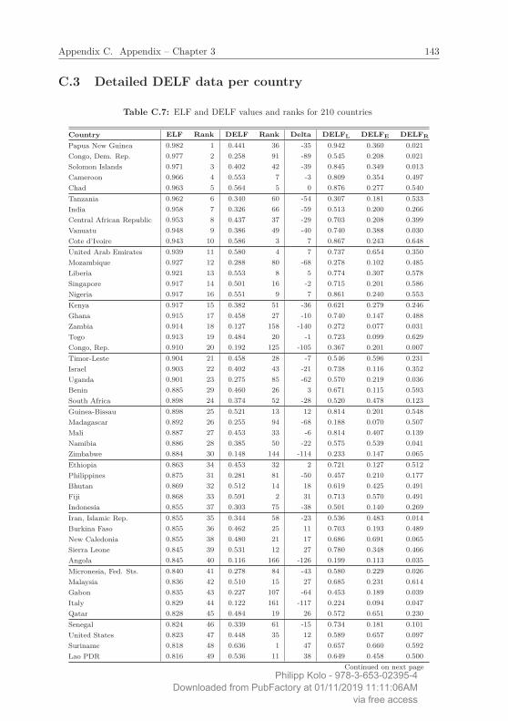
Appendix C. Appendix – Chapter 3 143
C.3 Detailed DELF data per country
Table C.7: ELF and DELF values and ranks for 210 countries
Country ELF Rank DELF Rank Delta DELFL DELFE DELFR
Papua New Guinea 0.982 1 0.441 36 -35 0.942 0.360 0.021Congo, Dem. Rep. 0.977 2 0.258 91 -89 0.545 0.208 0.021Solomon Islands 0.971 3 0.402 42 -39 0.845 0.349 0.013Cameroon 0.966 4 0.553 7 -3 0.809 0.354 0.497Chad 0.963 5 0.564 5 0 0.876 0.277 0.540Tanzania 0.962 6 0.340 60 -54 0.307 0.181 0.533India 0.958 7 0.326 66 -59 0.513 0.200 0.266Central African Republic 0.953 8 0.437 37 -29 0.703 0.208 0.399Vanuatu 0.948 9 0.386 49 -40 0.740 0.388 0.030Cote d’Ivoire 0.943 10 0.586 3 7 0.867 0.243 0.648United Arab Emirates 0.939 11 0.580 4 7 0.737 0.654 0.350Mozambique 0.927 12 0.288 80 -68 0.278 0.102 0.485Liberia 0.921 13 0.553 8 5 0.774 0.307 0.578Singapore 0.917 14 0.501 16 -2 0.715 0.201 0.586Nigeria 0.917 16 0.551 9 7 0.861 0.240 0.553Kenya 0.917 15 0.382 51 -36 0.621 0.279 0.246Ghana 0.915 17 0.458 27 -10 0.740 0.147 0.488Zambia 0.914 18 0.127 158 -140 0.272 0.077 0.031Togo 0.913 19 0.484 20 -1 0.723 0.099 0.629Congo, Rep. 0.910 20 0.192 125 -105 0.367 0.201 0.007Timor-Leste 0.904 21 0.458 28 -7 0.546 0.596 0.231Israel 0.903 22 0.402 43 -21 0.738 0.116 0.352Uganda 0.901 23 0.275 85 -62 0.570 0.219 0.036Benin 0.885 29 0.460 26 3 0.671 0.115 0.593South Africa 0.898 24 0.374 52 -28 0.520 0.478 0.123Guinea-Bissau 0.898 25 0.521 13 12 0.814 0.201 0.548Madagascar 0.892 26 0.255 94 -68 0.188 0.070 0.507Mali 0.887 27 0.453 33 -6 0.814 0.407 0.139Namibia 0.886 28 0.385 50 -22 0.575 0.539 0.041Zimbabwe 0.884 30 0.148 144 -114 0.233 0.147 0.065Ethiopia 0.863 34 0.453 32 2 0.721 0.127 0.512Philippines 0.875 31 0.281 81 -50 0.457 0.210 0.177Bhutan 0.869 32 0.512 14 18 0.619 0.425 0.491Fiji 0.868 33 0.591 2 31 0.713 0.570 0.491Indonesia 0.855 37 0.303 75 -38 0.501 0.140 0.269Iran, Islamic Rep. 0.855 35 0.344 58 -23 0.536 0.483 0.014Burkina Faso 0.855 36 0.462 25 11 0.703 0.193 0.489New Caledonia 0.855 38 0.480 21 17 0.686 0.691 0.065Sierra Leone 0.845 39 0.531 12 27 0.780 0.348 0.466Angola 0.845 40 0.116 166 -126 0.199 0.113 0.035Micronesia, Fed. Sts. 0.840 41 0.278 84 -43 0.580 0.229 0.026Malaysia 0.836 42 0.510 15 27 0.685 0.231 0.614Gabon 0.835 43 0.227 107 -64 0.453 0.189 0.039Italy 0.829 44 0.122 161 -117 0.224 0.094 0.047Qatar 0.828 45 0.484 19 26 0.572 0.651 0.230Senegal 0.824 46 0.339 61 -15 0.734 0.181 0.101United States 0.823 47 0.448 35 12 0.589 0.657 0.097Suriname 0.818 48 0.636 1 47 0.657 0.660 0.592Lao PDR 0.816 49 0.536 11 38 0.649 0.458 0.500
Continued on next pagePhilipp Kolo - 978-3-653-02395-4
Downloaded from PubFactory at 01/11/2019 11:11:06AMvia free access

144 Appendix C. Appendix – Chapter 3
Table C.7 – continued from previous pageCountry ELF Rank DELF Rank Delta DELFL DELFE DELFR
Niger 0.782 58 0.396 45 13 0.728 0.353 0.108Brunei Darussalam 0.809 50 0.480 22 28 0.679 0.143 0.620Malawi 0.807 51 0.138 148 -97 0.154 0.062 0.197Mauritius 0.807 52 0.560 6 46 0.609 0.518 0.551Peru 0.803 53 0.336 63 -10 0.421 0.576 0.010France 0.802 54 0.336 62 -8 0.453 0.355 0.202N. Mariana Islands 0.798 55 0.396 46 9 0.775 0.385 0.028Thailand 0.793 56 0.216 113 -57 0.304 0.155 0.189Belgium 0.782 57 0.314 69 -12 0.560 0.290 0.091Belize 0.779 59 0.494 18 41 0.677 0.708 0.096Kuwait 0.777 60 0.363 56 4 0.446 0.434 0.209Pakistan 0.777 61 0.243 102 -41 0.410 0.299 0.021Gambia, The 0.774 62 0.390 48 14 0.745 0.311 0.113Afghanistan 0.774 63 0.297 78 -15 0.500 0.388 0.003Morocco 0.770 64 0.187 128 -64 0.464 0.097 0.002Monaco 0.765 65 0.190 127 -62 0.296 0.228 0.045Oman 0.759 66 0.474 23 43 0.634 0.574 0.212Guinea 0.753 67 0.464 24 43 0.647 0.233 0.512Canada 0.751 68 0.419 40 28 0.632 0.455 0.171Mauritania 0.750 69 0.265 90 -21 0.412 0.378 0.004Bolivia 0.749 70 0.431 38 32 0.678 0.572 0.043Spain 0.745 71 0.195 120 -49 0.313 0.240 0.032Nepal 0.744 72 0.390 47 25 0.446 0.388 0.336Sudan 0.738 73 0.538 10 63 0.664 0.534 0.417Ecuador 0.737 74 0.307 73 1 0.282 0.627 0.013Latvia 0.728 75 0.250 97 -22 0.510 0.226 0.014Eritrea 0.721 76 0.398 44 32 0.508 0.189 0.498Guyana 0.707 77 0.457 29 48 0.248 0.600 0.522Nauru 0.705 78 0.449 34 44 0.690 0.432 0.226Myanmar 0.699 79 0.420 39 40 0.589 0.264 0.408Trinidad and Tobago 0.698 80 0.410 41 39 0.188 0.559 0.483Andorra 0.693 81 0.137 149 -68 0.213 0.164 0.034Cayman Islands 0.686 82 0.253 96 -14 0.237 0.480 0.043Bosnia and Herzegovina 0.686 83 0.351 57 26 0.273 0.281 0.499Guam 0.679 84 0.343 59 25 0.645 0.325 0.061Switzerland 0.677 85 0.317 68 17 0.572 0.274 0.106Colombia 0.677 86 0.224 109 -23 0.050 0.609 0.012Montenegro 0.671 87 0.223 110 -23 0.219 0.167 0.283Guatemala 0.668 88 0.364 55 33 0.571 0.522 0.000New Zealand 0.667 89 0.366 53 36 0.505 0.491 0.103French Polynesia 0.661 90 0.258 93 -3 0.447 0.325 0.001Brazil 0.660 91 0.216 114 -23 0.048 0.591 0.008Mexico 0.658 92 0.249 98 -6 0.168 0.575 0.005Equatorial Guinea 0.655 93 0.266 88 5 0.543 0.214 0.042Djibouti 0.644 94 0.279 83 11 0.619 0.180 0.037Algeria 0.635 95 0.156 139 -44 0.401 0.065 0.003Iraq 0.633 96 0.326 65 31 0.454 0.489 0.036Estonia 0.631 97 0.299 77 20 0.449 0.437 0.010Luxembourg 0.620 98 0.248 101 -3 0.468 0.250 0.028Panama 0.616 99 0.366 54 45 0.465 0.584 0.048Macedonia, FYR 0.613 100 0.456 30 70 0.578 0.332 0.459Grenada 0.611 101 0.116 165 -64 0.156 0.193 0.000
Continued on next page
Philipp Kolo - 978-3-653-02395-4Downloaded from PubFactory at 01/11/2019 11:11:06AM
via free access

Appendix C. Appendix – Chapter 3 145
Table C.7 – continued from previous pageCountry ELF Rank DELF Rank Delta DELFL DELFE DELFR
Kazakhstan 0.603 102 0.499 17 85 0.513 0.487 0.498St. Lucia 0.600 103 0.133 154 -51 0.197 0.168 0.033China 0.594 104 0.234 105 -1 0.223 0.035 0.445Egypt, Arab Rep. 0.589 105 0.065 185 -80 0.086 0.099 0.008Georgia 0.586 106 0.311 71 35 0.506 0.272 0.155Greenland 0.581 107 0.241 103 4 0.385 0.338 0.000Bahrain 0.576 108 0.455 31 77 0.548 0.522 0.296Nicaragua 0.575 109 0.301 76 33 0.371 0.524 0.008Bermuda 0.574 110 0.192 124 -14 0.138 0.438 0.001Virgin Islands (U.S.) 0.570 111 0.309 72 39 0.437 0.470 0.020Comoros 0.567 112 0.041 192 -80 0.057 0.025 0.042Mongolia 0.506 125 0.266 89 36 0.191 0.083 0.523Turkey 0.560 113 0.255 95 18 0.328 0.430 0.006Mayotte 0.545 114 0.335 64 50 0.495 0.492 0.019Netherlands 0.542 115 0.215 115 0 0.261 0.237 0.147Venezuela, RB 0.542 116 0.194 122 -6 0.059 0.484 0.040Kyrgyz Republic 0.539 117 0.291 79 38 0.334 0.297 0.242Albania 0.539 118 0.248 100 18 0.334 0.140 0.272Ireland 0.539 119 0.194 123 -4 0.488 0.073 0.020Australia 0.534 120 0.305 74 46 0.381 0.354 0.178Sri Lanka 0.503 126 0.312 70 56 0.440 0.060 0.437Bahamas, The 0.523 121 0.146 145 -24 0.220 0.215 0.002Germany 0.518 122 0.165 135 -13 0.242 0.156 0.096Tajikistan 0.510 123 0.325 67 56 0.467 0.449 0.058St. Vincent & the Gr. 0.508 124 0.199 117 7 0.210 0.272 0.113Sweden 0.503 127 0.179 130 -3 0.255 0.207 0.074Chile 0.500 128 0.219 112 16 0.213 0.439 0.004Norway 0.492 129 0.133 152 -23 0.202 0.124 0.072Cape Verde 0.488 130 0.270 87 43 0.446 0.364 0.000Liechtenstein 0.485 131 0.225 108 23 0.300 0.211 0.165Dominican Republic 0.481 132 0.130 156 -24 0.048 0.340 0.003Tuvalu 0.471 133 0.058 187 -54 0.141 0.033 0.000United Kingdom 0.470 134 0.176 132 2 0.244 0.183 0.101Bangladesh 0.341 153 0.098 172 -19 0.050 0.039 0.204Botswana 0.462 136 0.158 137 -1 0.175 0.137 0.162Tunisia 0.464 135 0.038 194 -59 0.107 0.006 0.002Cuba 0.449 137 0.281 82 55 0.018 0.417 0.407Puerto Rico 0.446 138 0.157 138 0 0.048 0.419 0.005Argentina 0.444 139 0.249 99 40 0.245 0.412 0.089Moldova 0.444 140 0.198 118 22 0.395 0.173 0.027Palau 0.437 141 0.258 92 49 0.401 0.373 0.000Netherlands Antilles 0.426 142 0.200 116 26 0.337 0.233 0.029Saudi Arabia 0.420 143 0.197 119 24 0.263 0.243 0.086Libya 0.415 144 0.117 164 -20 0.172 0.139 0.039Ukraine 0.403 145 0.094 174 -29 0.115 0.110 0.057Aruba 0.399 146 0.191 126 20 0.222 0.337 0.013Uzbekistan 0.375 147 0.155 140 7 0.207 0.180 0.078Russian Federation 0.374 148 0.271 86 62 0.328 0.272 0.215Somalia 0.372 149 0.079 178 -29 0.147 0.063 0.026Jamaica 0.364 150 0.087 176 -26 0.081 0.130 0.050Costa Rica 0.363 151 0.136 150 1 0.083 0.308 0.018Bulgaria 0.337 156 0.232 106 50 0.228 0.278 0.190Turkmenistan 0.344 152 0.121 162 -10 0.151 0.136 0.076
Continued on next pagePhilipp Kolo - 978-3-653-02395-4
Downloaded from PubFactory at 01/11/2019 11:11:06AMvia free access

146 Appendix C. Appendix – Chapter 3
Table C.7 – continued from previous pageCountry ELF Rank DELF Rank Delta DELFL DELFE DELFR
Syrian Arab Republic 0.340 154 0.152 141 13 0.217 0.204 0.033Dominica 0.337 155 0.110 169 -14 0.199 0.129 0.002Austria 0.332 157 0.151 142 15 0.221 0.145 0.085Belarus 0.329 158 0.041 193 -35 0.053 0.057 0.013Barbados 0.324 159 0.122 160 -1 0.107 0.236 0.024Jordan 0.321 160 0.057 188 -28 0.082 0.066 0.023Serbia 0.318 161 0.171 133 28 0.214 0.194 0.106Vietnam 0.309 162 0.221 111 51 0.265 0.149 0.250Paraguay 0.308 163 0.179 129 34 0.269 0.252 0.016Lesotho 0.308 164 0.034 195 -31 0.061 0.039 0.002American Samoa 0.307 165 0.135 151 14 0.277 0.115 0.014Uruguay 0.305 166 0.133 153 13 0.085 0.279 0.034Greece 0.304 167 0.166 134 33 0.261 0.132 0.104Swaziland 0.304 168 0.064 186 -18 0.098 0.078 0.016Lebanon 0.302 169 0.239 104 65 0.276 0.259 0.183Hungary 0.290 170 0.178 131 39 0.223 0.285 0.026Lithuania 0.284 171 0.132 155 16 0.269 0.120 0.008Honduras 0.270 172 0.129 157 15 0.124 0.257 0.006West Bank and Gaza 0.266 173 0.150 143 30 0.155 0.052 0.243Antigua and Barbuda 0.262 174 0.093 175 -1 0.072 0.198 0.008Croatia 0.248 175 0.097 173 2 0.150 0.121 0.021Slovak Republic 0.247 176 0.142 147 29 0.207 0.217 0.001Azerbaijan 0.244 177 0.145 146 31 0.177 0.173 0.086Cambodia 0.233 178 0.195 121 57 0.219 0.203 0.163Isle of Man 0.222 179 0.027 204 -25 0.015 0.064 0.002Kosovo 0.220 180 0.163 136 44 0.214 0.099 0.175Romania 0.216 181 0.124 159 22 0.173 0.191 0.008El Salvador 0.215 182 0.104 170 12 0.106 0.204 0.001Marshall Islands 0.210 183 0.111 168 15 0.122 0.210 0.000Samoa 0.210 184 0.086 177 7 0.207 0.051 0.000Yemen, Rep. 0.195 185 0.074 180 5 0.137 0.063 0.023Slovenia 0.192 186 0.054 190 -4 0.079 0.046 0.037Finland 0.177 187 0.101 171 16 0.146 0.142 0.015Cyprus 0.173 188 0.112 167 21 0.170 0.123 0.042Portugal 0.173 189 0.074 181 8 0.056 0.144 0.023Denmark 0.165 190 0.117 163 27 0.144 0.122 0.086San Marino 0.164 191 0.010 207 -16 0.029 0.002 0.000St. Kitts and Nevis 0.153 192 0.073 182 10 0.066 0.105 0.049Sao Tome and Principe 0.153 193 0.052 191 2 0.058 0.098 0.000Rwanda 0.147 194 0.032 198 -4 0.013 0.044 0.039Iceland 0.141 195 0.054 189 6 0.107 0.052 0.004Malta 0.119 196 0.073 183 13 0.110 0.108 0.001Seychelles 0.117 197 0.070 184 13 0.087 0.110 0.014Czech Republic 0.109 198 0.033 197 1 0.050 0.042 0.006Haiti 0.108 199 0.010 208 -9 0.008 0.021 0.001Poland 0.102 200 0.033 196 4 0.065 0.035 0.001Armenia 0.100 201 0.077 179 22 0.099 0.090 0.042Burundi 0.099 202 0.028 202 0 0.022 0.038 0.025Tonga 0.094 203 0.031 200 3 0.055 0.035 0.004Korea, Rep. 0.059 204 0.032 199 5 0.045 0.009 0.041Maldives 0.059 205 0.028 203 2 0.043 0.018 0.022Faeroe Islands 0.058 206 0.006 210 -4 0.010 0.009 0.000
Continued on next page
Philipp Kolo - 978-3-653-02395-4Downloaded from PubFactory at 01/11/2019 11:11:06AM
via free access

Appendix C. Appendix – Chapter 3 147
Table C.7 – continued from previous pageCountry ELF Rank DELF Rank Delta DELFL DELFE DELFR
Channel Islands 0.055 207 0.029 201 6 0.053 0.029 0.005Kiribati 0.050 208 0.021 205 3 0.050 0.014 0.000Japan 0.048 209 0.019 206 3 0.032 0.011 0.014Korea, Dem. Rep. 0.019 210 0.007 209 1 0.015 0.006 0.000
Philipp Kolo - 978-3-653-02395-4Downloaded from PubFactory at 01/11/2019 11:11:06AM
via free access
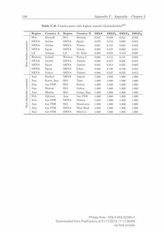
148 Appendix C. Appendix – Chapter 3
Table C.8: Country-pairs with highest mutual (dis)similarities267
Region Country A Region Country B DELF DELFL DELFE DELFR
Mostsim
ilarcountries
SSA Burundi SSA Rwanda 0.047 0.068 0.041 0.032MENA Jordan MENA Egypt 0.072 0.118 0.083 0.015MENA Jordan MENA Yemen. 0.081 0.155 0.065 0.023MENA Egypt MENA Yemen 0.083 0.151 0.082 0.015LA Antigua LA St. Kitts 0.085 0.070 0.155 0.029Western Iceland Western Faeroe I. 0.086 0.115 0.141 0.002MENA Jordan MENA Tunisia 0.089 0.217 0.037 0.012MENA Egypt MENA Tunisia 0.091 0.214 0.055 0.005MENA Egypt MENA Libya 0.093 0.136 0.120 0.024MENA Yemen MENA Tunisia 0.098 0.247 0.035 0.012
Mostdissimilarcountries
Asia Kiribati MENA Algeria 1.000 1.000 1.000 1.000Asia Korea, Rep. SSA Niger 1.000 1.000 1.000 1.000Asia Lao PDR SSA Eritrea 1.000 1.000 1.000 1.000Asia Bhutan SSA Gabon 1.000 1.000 1.000 1.000Asia Bhutan SSA Congo, Rep. 1.000 1.000 1.000 1.000SSA Djibouti Asia Lao PDR 1.000 1.000 1.000 1.000Asia Lao PDR MENA Tunisia 1.000 1.000 1.000 1.000Asia Lao PDR SSA Mauritania 1.000 1.000 1.000 1.000Asia Lao PDR MENA West Bank 1.000 1.000 1.000 1.000Asia Lao PDR MENA Morocco 1.000 1.000 1.000 1.000
Philipp Kolo - 978-3-653-02395-4Downloaded from PubFactory at 01/11/2019 11:11:06AM
via free access

Appendix C. Appendix – Chapter 3 149
Tabl
eC
.9:DetailsofEU
enlargem
entwa
vesandrespectiv
eD
EL
Faverages
Enl
arge
men
tw
aves
Pot
enti
alfu
ture
enla
rgem
ent
EU
grou
pE
U6
EU
9E
U10
EU
12E
U15
EU
25E
U27
EU
+B
EU
+T
EU
+B
+T
Year
1952
1973
1981
1986
1995
2004
2007
––
–
Countries
Belgium
Denmark
Greece
Portugal
Austria
Cyprus
Bulgaria
Albania
Turkey
Albania
France
Ireland
Spain
Finland
Czech
Rep.
Rom
ania
Croatia
Croatia
Germany
Britain
Sweden
Estonia
Iceland
Iceland
Italy
Hungary
Macedonia
Macedonia
Luxembourg
Latvia
Montenegro
Montenegro
Netherla
nds
Lithuania
Serbia
Serbia
Malta
Turkey
Poland
Slovak
Rep.
Slovenia
DEL
F0.3685
0.3875
0.3940
0.3893
0.3987
0.4196
0.4206
0.4263
0.5383
0.5393
Del
ta0.
019
0.00
6-0
.005
0.00
90.
021
0.00
10.
006
0.11
80.
119
Philipp Kolo - 978-3-653-02395-4Downloaded from PubFactory at 01/11/2019 11:11:06AM
via free access

Philipp Kolo - 978-3-653-02395-4Downloaded from PubFactory at 01/11/2019 11:11:06AM
via free access

Appendix D
Appendix – Chapter 4
D.1 Summary statistics for all replications
Table D.1: Summary statistics for replications of Garcia-Montalvo and Reynal-Querol (2005b)
Variable Obs. Mean Std. Dev. Min. Max.Conflict 1,096 0.145 0.352 0.000 1.000Ethnic fractionalization 1,096 0.442 0.277 0.010 0.959Ethnic polarization 1,096 0.516 0.248 0.017 0.982Religious fractionalization 1,096 0.284 0.235 0.001 0.782Religious polarization 1,096 0.468 0.356 0.001 1.000Ln (GDP/capita) 1,016 7.733 1.046 5.416 10.710Ln (Population) 1,092 15.390 1.951 10.638 20.908Primary exports 1,039 0.166 0.185 0.002 2.139Mountains 1,088 15.311 20.074 0.000 82.200Non contiguous 1,096 0.155 0.361 0.000 1.000Democracy 896 0.459 0.499 0.000 1.000
Philipp Kolo - 978-3-653-02395-4Downloaded from PubFactory at 01/11/2019 11:11:06AM
via free access

152 Appendix D. Appendix – Chapter 4
Table D.2: Summary statistics for replications of Schüler and Weisbrod (2010)
Variable Obs. Mean Std. Dev. Min. Max.Growth 476 0.018 0.027 -0.085 0.173Africa 640 0.294 0.456 0.000 1.000Latin America 640 0.238 0.426 0.000 1.000Ln (GDP/cap.) 460 7.741 1.035 5.438 10.053(Ln (GDP/cap.))2 460 60.995 16.269 29.573 101.056Ln (Schooling) 399 1.518 0.588 0.039 2.576Assassinations 476 0.000 0.000 0.000 0.001Financial depth 445 0.395 0.322 0.002 2.977Black market premium 505 0.236 0.406 -0.064 3.181Fiscal surplus/GDP 413 -0.234 4.102 -83.393 0.112Ln (Telephones/worker) 553 1.266 0.898 -1.398 2.860ELF (Alesina) 584 0.439 0.274 0.000 0.930
Table D.3: Summary statistics for replications of Bjørnskov (2008)
Variable Obs. Mean Std. Dev. Min. Max.Trust 116 25.483 13.466 3.400 68.076Income inequality 113 41.391 11.371 21.500 70.700Post communist 116 0.216 0.413 0.000 1.000Monarchy 116 0.164 0.372 0.000 1.000Nordic country 116 0.043 0.204 0.000 1.000Politial diversity 89 5.149 1.860 2.074 12.066Political competition (’80–’05) 112 0.542 0.211 0.132 1.000Protestant 116 15.022 23.779 0.000 95.000Muslim 214 10.672 25.250 0.000 100.000Catholic 116 30.266 36.561 0.000 98.000Eastern 116 5.776 19.733 0.000 95.100ELF (Alesina) 116 0.397 0.240 0.002 0.930
Philipp Kolo - 978-3-653-02395-4Downloaded from PubFactory at 01/11/2019 11:11:06AM
via free access

Appendix D. Appendix – Chapter 4 153
Table D.4: Summary statistics for replications of Disdier and Mayer (2007)
Variable Obs. Mean Std. Dev. Min. Max.Opinion 887 -0.239 0.529 -1.992 1.208Language proximity 1,960 0.179 0.097 0.000 0.456Religion proximity 1,960 0.373 0.202 0.073 0.843Asylum seekers 1,540 1.443 1.403 0.000 4.615Book imports 1,960 2.225 8.057 -4.605 16.872Conflict years 1,960 2.064 3.248 0.000 12.000UN voting 1,960 4.438 0.088 4.193 4.585Ln (Exports) 1,287 -24.720 1.253 -31.859 -19.884Ln (Imports) 1,287 -24.932 1.233 -32.797 -20.240GDP/cap. differences 1,400 9.695 0.505 6.844 10.402EU budget contribution 1,310 -0.757 1.615 -5.826 0.641EC benefits 1,750 3.971 0.329 2.890 4.500Ln (Distance) 1,960 7.164 0.527 5.479 8.106Common border 1,960 0.057 0.232 0.000 1.000Newspaper imports 1,960 -2.807 4.966 -4.605 16.396
Table D.5: Summary statistics for replications of Felbermayr and Toubal (2010)
Variable Obs. Mean Std. Dev. Min. Max.Aggregate imports 10,560 19.096 2.540 7.084 25.081Aggregate imports (hom. goods) 7,161 16.609 2.398 6.908 23.066Aggregate imports (diff. goods) 7,826 18.490 2.409 8.006 24.282Common law 10,560 0.183 0.387 0.000 1.000Common language 10,560 0.061 0.240 0.000 1.000Religion proximity 10,560 0.210 0.248 0.001 0.854Ethnic ties 10,457 7.816 2.742 0.000 15.433Common FTA 10,560 0.308 0.462 0.000 1.000Ln (Distance) 10,560 7.306 0.627 4.394 8.565Common border 10,560 0.091 0.287 0.000 1.000ESCij 12,356 0.259 0.330 0.000 1.000ESCji 12,356 0.259 0.330 0.000 1.000
Philipp Kolo - 978-3-653-02395-4Downloaded from PubFactory at 01/11/2019 11:11:06AM
via free access

154 Appendix D. Appendix – Chapter 4
D.2 Marginal effects of DELF
Figure D.1: Average marginal effects of DELF dependent on HDI levels with 90% confidenceintervalls for regressions (4) and (5) of Table 4.4
(a) Regression (4)
(b) Regression (5)
Philipp Kolo - 978-3-653-02395-4Downloaded from PubFactory at 01/11/2019 11:11:06AM
via free access

Bibliography
Acemoglu, D., Johnson, S. and Robinson, J. A. (2001). The Colonial Origins of Compar-ative Development: An Empirical Investigation. The American Economic Review 91:1369–1401.
Ahlerup, P. and Olsson, O. (2007). The Roots of Ethnic Diversity. Working Papers inEconomics 281, Department of Economics, Göteborg University.
Akdede, S. H. (2010). Do more Ethnically and Religiously Diverse Countries have LowerDemocratization? Economics Letters 106: 101–104.
Akerlof, G. A. and Kranton, R. E. (2000). Economics and Identity. The Quarterly Journalof Economics 115: 715–753.
Alesina, A., Baqir, R. and Easterly, W. (1999). Public Goods and Ethnic Divisions. TheQuarterly Journal of Economics 114: 1243–1284.
Alesina, A., Devleeschauwer, A., Easterly, W., Kurlat, S. and Wacziarg, R. (2003). Frac-tionalization. Journal of Economic Growth 8: 155–194.
Alesina, A., Easterly, W. and Matuszeski, J. (2011). Artificial States. Journal of the Eu-ropean Economic Association 9: 246–277.
Alesina, A. and La Ferrara, E. (2000). Participation in Heterogeneous Communities. TheQuarterly Journal of Economics 115: 847–904.
Alesina, A. and La Ferrara, E. (2002). Who Trusts Others? Journal of Public Economics85: 207–234.
Alesina, A. and La Ferrara, E. (2005). Ethnic Diversity and Economic Performance. Jour-nal of Economic Literature 43: 762–800.
Alesina, A. and Zhuravskaya, E. (2011). Segregation and the Quality of Government in aCross-Section of Countries. The American Economic Review 101: 1872–1911.
Annett, A. (2001). Social Fractionalization, Political Instability, and the Size of Govern-ment. IMF Staff Papers 48: 561–592.
Ashraf, Q. and Galor, O. (2007). Cultural Assimilation, Cultural Diffusion and the Originof the Wealth of Nations. CEPR Discussion Papers 6444, Center for Economic PolicyResearch.
Ashraf, Q. and Galor, O. (2011). The ”Out of Africa” Hypothesis, Human Genetic Diver-sity, and Comparative Economic Development. NBER Working Papers 17216, NationalBureau of Economic Research (NBER).
Philipp Kolo - 978-3-653-02395-4Downloaded from PubFactory at 01/11/2019 11:11:06AM
via free access

156 Bibliography
Aspachs-Bracons, O., Clots-Figueras, I. and Masella, P. (2007a). Education and PoliticalBehaviour: Evidence from the Catalan Linguistic Reform. Economics Working Papers07-78, Universidad Carlos III de Madrid.
Aspachs-Bracons, O., Clots-Figueras, I. and Masella, P. (2007b). Identity and LanguagePolicies. Economics Working Papers 07-78, Universidad Carlos III de Madrid.
Auer, R. (2009). The Colonial and Geographic Origins of Comparative Development.Working Papers 09.03, Swiss National Bank, Study Center Gerzensee.
Bannon, A., Miguel, E. and Posner, D. N. (2004). Sources of Ethnic Identification inAfrica. Afrobarometer Working Papers 44, Afrobarometer.
Barrett, D. B., Kurian, G. T. and Johnson, T. M. (2001). World Christian Encyclopedia;A Comparative Survey of Churches and Religions in the Modern World. Oxford: OxfordUniversity Press, 2nd ed.
Barro, R. J. (1999). Determinants of Democracy. Journal of Political Economy 107: 158–183.
Barro, R. J. and Lee, J.-W. (2010). A New Data Set of Educational Attainment in theWorld, 1950-2010. NBER Working Papers 15902, National Bureau of Economic Re-search (NBER).
Barro, R. J. and McCleary, R. M. (2003). Religion and Economic Growth. NBER WorkingPapers 9682, National Bureau of Economic Research (NBER).
Bates, R. H. (2006). Ethnicity. In Clark, D. A. (ed.), The Elgar Companion to DevelopmentStudies. Cheltenham: Edward Elgar Publishing, 167–173.
Beine, M., Docquier, F. and Özden, C. (2011). Diasporas. Journal of Development Eco-nomics 95: 30–41.
Bellini, E., Ottaviano, G. I. P., Pinelli, D. and Prarolo, G. (2009). Cultural Diversity andEconomic Performance: Evidence from European Regions. Working Papers 2009.63,Fondazione Eni Enrico Mattei.
Belloc, M. and Bowles, S. (2009). International Trade, Factor Mobility and the Persistenceof Cultural-Institutional Diversity. CESifo Working Paper Series 2762, CESifo GroupMunich.
Berghe, P. L. van den (1981). The Ethnic Phenomenon. New York: Elsevier.
Bisin, A. and Verdier, T. (2001). The Economics of Cultural Transmission and the Dy-namics of Preferences. Journal of Economic Theory 97: 298–319.
Bjørnskov, C. (2007). Determinants of Generalized Trust: A Cross-country Comparison.Public Choice 130: 1–21.
Bjørnskov, C. (2008). Social Trust and Fractionalization: A Possible Reinterpretation.European Sociological Review 24: 271–283.
Blattman, C. and Miguel, E. (2010). Civil War. Journal of Economic Literature 48: 3–57.Philipp Kolo - 978-3-653-02395-4
Downloaded from PubFactory at 01/11/2019 11:11:06AMvia free access

Bibliography 157
Bleaney, M. and Dimico, A. (2009). Incidence, Onset and Duration of Civil Wars: AReview of the Evidence. CREDIT Research Paper 09/08, University of Nottingham.
Bodenhorn, H. and Ruebeck, C. S. (2003). The Economics of Identity and the Endogeneityof Race. NBER Working Papers 9962, National Bureau of Economic Research (NBER).
Bolt, J. and Bezemer, D. (2009). Understanding Long-Run African Growth: ColonialInstitutions or Colonial Education? The Journal of Development Studies 45: 24–54.
Booysen, F. (2002). An Overview and Evaluation of Composite Indices of Development.Social Indicators Research 59: 115–151.
Bossert, W., D’Ambrosio, C. and La Ferrara, E. (2011). A Generalized Index of Fraction-alization. Economica 78: 723–750.
Bossert, W., Pattanaik, P. K. and Xu, Y. (2003). Similarity of Options and the Measure-ment of Diversity. Journal of Theoretical Politics 15: 405–421.
Bossuroy, T. (2011). Ethnic Solidarity and the Individual Determinants of Ethnic Identi-fication. Economic Research Southern Africa Working Papers 242, University of CapeTown.
Branisa, B., Klasen, S. and Ziegler, M. (2009). The Construction of the Social Institutionsand Gender Index (SIGI). Discussion Papers 184, Ibero America Institute for EconomicResearch (IAI), Georg-August-Universität Göttingen.
Brown, G. K. and Langer, A. (2010). Conceptualizing and Measuring Ethnicity. OxfordDevelopment Studies 38: 411–436.
Bruk, S. I. (1964). Atlas Narodov Mira. Moskva: N. N. Miklucho-Maklaja, Institut Etno-grafii Imeni.
Bruk, S. I. and Pučkov, P. I. (1986). Naselenie Mira. Moskva: Nauka, 2nd ed., Etnode-mografičeskij Spravočnik.
Cahill, M. B. (2005). Is the Human Development Index Redundant? Social IndicatorsResearch 31: 1–5.
Campos, N. F. and Kuzeyev, V. S. (2007). On the Dynamics of Ethnic Fractionalization.American Journal of Political Science 51: 620–639.
Carvalho, J.-P. (2010). Coordination and Culture. Economics Series Working Papers 489,Department of Economics, University of Oxford.
Caselli, F. and Coleman, W. J. (2008). On the Theory of Ethnic Conflict. CEDI Dis-cussion Paper Series 08-08, Centre for Economic Development and Institutions, BrunelUniversity West London.
Cashdan, E. (2001). Ethnic Diversity and its Environmental Determinants: Effects ofClimate, Pathogens, and Habitat Diversity. American Anthropologist 103: 968–991.
Cavalli-Sforza, L. L. and Feldmann, M. W. (1981). Cultural Transmission and Evolution;A Quantitative Approach. Princeton, NJ: Princeton University Press.
Philipp Kolo - 978-3-653-02395-4Downloaded from PubFactory at 01/11/2019 11:11:06AM
via free access

158 Bibliography
Cavalli-Sforza, L. L., Menozzi, P. and Piazza, A. (1993). The History and Geography ofHuman Genes. Princeton, NJ: Princeton University Press.
Cavalli-Sforza, L. L., Piazza, A., Menozzi, P. and Mountain, J. (1988). Reconstructionof Human Evolution: Bringing Together Genetic, Archaeological, and Linguistic Data.Proceedings of the National Academy of Sciences of the United States of America 85:6002–6006.
Chai, S.-K. (2005). Predicting Ethnic Boundaries. European Sociological Review 21: 375–391.
Chandra, K. and Wilkinson, S. (2008). Measuring the Effect of ‘Ethnicity’. ComparativePolitical Studies 41: 515–563.
Chiswick, B. R. and Miller, P. W. (2007). The Economics of Language: InternationalAnalyses, Routledge Studies in the Modern World Economy 65 . London: Routledge.
Cho, S.-Y., Dreher, A. and Neumayer, E. (2011). The Spread of Anti-Trafficking Policies -Evidence from a New Index. CESifo Working Paper Series 3376, CESifo Group Munich.
Chong, A., Guillen, J. and Rios, V. (2010). Language Nuances, Trust and EconomicGrowth. Public Choice 143: 191–208.
Chowdhury, S. and Squire, L. (2006). Setting Weights for Aggregate Indices: An Appli-cation to the Commitment to Development Index and Human Development Index. TheJournal of Development Studies 42: 761–771.
Christofides, L. N. and Swidinsky, R. (2010). The Economic Returns to the Knowledgeand Use of a Second Official Language: English in Quebec and French in the Rest-of-Canada. Working Papers in Economics 04-2010, University of Cyprus.
Church, J. and King, I. (1993). Bilingualism and Network Externalities. Canadian Journalof Economics 26: 337–345.
CIA (2011). The World Factbook. https://www.cia.gov/library/publications/the-world-factbook/.
Clévenot, M. (1987). L’ Etat des Religions dans le Monde. Paris: La Découverte.
Coleman, D. (2009). Divergent Patterns in the Ethnic Transformation of Societies. Popu-lation and Development Review 35: 449–478.
Collier, P. (1998). The Political Economy of Ethnicity. Working Paper Series 98-8, Centrefor the Study of African Economies, University of Oxford.
Collier, P. (2000). Ethnicity, Politics and Economic Performance. Economics and Politics12: 225–245.
Collier, P. (2001). Implications of Ethnic Diversity. Economic Policy 16: 129–155.
Collier, P. and Hoeffler, A. (1998). On Economic Causes of Civil War. Oxford EconomicPapers 50: 563–573.
Collier, P. and Hoeffler, A. (2002). On the Incidence of Civil War in Africa. The Journalof Conflict Resolution 46: 13–28.
Philipp Kolo - 978-3-653-02395-4Downloaded from PubFactory at 01/11/2019 11:11:06AM
via free access

Bibliography 159
Collier, P. and Hoeffler, A. (2004). Greed and Grievance in Civil War. Oxford EconomicPapers 56: 563–595.
Collier, P., Hoeffler, A. and Rohner, D. (2009). Beyond Greed and Grievance: Feasibilityand Civil War. Oxford Economic Papers 61: 1–27.
Collier, P., Hoeffler, A. and Söderbom, M. (2004). On the Duration of Civil War. Journalof Peace Research 41: 253–273.
Combes, P.-P., Lafourcade, M. and Mayer, T. (2005). The Trade-creating Effects of Busi-ness and Social Networks: Evidence from France. Journal of International Economics66: 1–29.
Constant, A. F. and Zimmermann, K. F. (2007). Measuring Ethnic Identity and Its Impacton Economic Behavior. IZA Discussion Papers 3063, Institute for the Study of Labor(IZA).
Dalby, A. (2003). Language in Danger; the Loss of Linguistic Diversity and the Threat toour Future. New York: Columbia University Press.
Dalby, D. and Williams, C. (1999). The Linguasphere Register of the World’s Languagesand Speech Communities. Hebron, Wales: Linguasphere Press.
Danzer, A. M. and Yaman, F. (2010). Ethnic Concentration and Language Fluency ofImmigrants in Germany. SOEPpapers on Multidisciplinary Panel Data Research 277,DIW Berlin, German Institute for Economic Research.
D’Aquinas, T. (1873). Opera Omnia. Paris: Vivès.
Darity, W. A., JR., Mason, P. L. and Stewart, J. B. (2006). The Economics of Identity:The Origin and Persistence of Racial Identity Norms. Journal of Economic Behaviorand Organization 60: 283–305.
Desmet, K., Le Breton, M., Ortín, I. Ortuño and Weber, S. (2011). The Stability andBreakup of Nations: A Quantitative Analysis. Journal of Economic Growth 16: 183–213.
Desmet, K., Ortín, I. Ortuño and Wacziarg, R. (2012). The Political Economy of Ethno-linguistic Cleavages. Journal of Development Economics 97: 322–332.
Desmet, K., Ortín, I. Ortuño and Weber, S. (2009). Linguistic Diversity and Redistribu-tion. Journal of the European Economic Association 7: 1291–1318.
Diamond, J. M. (1997). Guns, Germs and Steel; The Fates of Human Societies. New York:W. W. Norton.
Disdier, A.-C. and Mayer, T. (2007). Je t’aime, moi non plus: Bilateral Opinions andInternational Trade. European Journal of Political Economy 23: 1140–1159.
Dreher, A. (2006). Does Globalization Affect Growth? Evidence from a New Index ofGlobalization. Applied Economics 38: 1091–1110.
Duclos, J.-Y., Esteban, J. and Ray, D. (2004). Polarization: Concepts, Measurement,Estimation. Econometrica 72: 1737–1772.
Philipp Kolo - 978-3-653-02395-4Downloaded from PubFactory at 01/11/2019 11:11:06AM
via free access

160 Bibliography
Easterly, W. (2001). Can Institutions Resolve Ethnic Conflict? Economic Developmentand Cultural Change 49: 687–706.
Easterly, W. and Levine, R. (1997). Africa’s Growth Tragedy: Policies and Ethnic Divi-sions. The Quarterly Journal of Economics 112: 1203–1250.
Eifert, B., Miguel, E. and Posner, D. N. (2007). Political Sources of Ethnic Identificationin Africa. Afrobarometer Working Papers 89, Afrobarometer.
Encyclopædia Britannica (ed.) (2007). The New Encyclopædia Britannica. Chicago [u.a.]:Encyclopædia Britannica Inc., 15th ed.
Eriksen, T. H. (1991). Ethnicity versus Nationalism. Journal of Peace Research 28: 263–278.
Esteban, J. and Mayoral, L. (2011). Ethnic and Religious Polarization and Social Conflict.Working paper 857.11, Unitat de Fonaments de l’Anàlisi Econòmica (UAB) and Institutd’Anàlisi Econòmica (CSIC).
Esteban, J., Mayoral, L. and Ray, D. (2010). Ethnicity and Conflict: An Empirical Study.Working Papers 840.10, Unitat de Fonaments de l’Anàlisi Econòmica (UAB) and Insti-tut d’Anàlisi Econòmica (CSIC).
Esteban, J. and Ray, D. (1994). On the Measurement of Polarization. Econometrica 62:819–851.
Esteban, J. and Ray, D. (2008). Polarization, Fractionalization and Conflict. Journal ofPeace Research 45: 163–182.
Esteban, J. and Ray, D. (2011). Linking Conflict to Inequality and Polarization. AmericanEconomic Review 101: 1345–1374.
European Commission (2006). Turkey 2006 Progress Report. Commission Staff WorkingDocument – SEC (2006) 1390. Brussels.
Evers, H.-D., Anis, Y. and Shamsul, A. B. (2010). Ethnic Diversity in Malaysia – LessonsLearned from Bio-Diversity Research. MPRA Paper 30383, University Library of Mu-nich.
Falck, O., Heblich, S., Lameli, A. and Suedekum, J. (2010). Dialects, Cultural Identity,and Economic Exchange. IZA Discussion Papers 4743, Institute for the Study of Labor(IZA).
Fearon, J. D. (2003). Ethnic and Cultural Diversity by Country. Journal of EconomicGrowth 8: 195–222.
Fearon, J. D. and Laitin, D. D. (1999). Weak States, Rough Terrain, and Large-scaleEthnic Violence since 1945. Presented at the Annual Meeting of the American PoliticalScience Association. Atlanta, Ga.
Fearon, J. D. and Laitin, D. D. (2000). Violence and the Social Construction of EthnicIdentity. International Organization 54: 845–877.
Fearon, J. D. and Laitin, D. D. (2003). Ethnicity, Insurgency, and Civil War. The AmericanPolitical Science Review 97: 75–90.
Philipp Kolo - 978-3-653-02395-4Downloaded from PubFactory at 01/11/2019 11:11:06AM
via free access

Bibliography 161
Fedderke, J., Luiz, J. and Kadt, R. de (2008). Using Fractionalization Indexes: Deriv-ing Methodological Principles for Growth Studies from Time Series Evidence. SocialIndicators Research 85: 257–278.
Fedderke, J. and Luiz, J. M. (2007). Fractionalization and Long-run Economic Growth:Webs and Direction of Association Between the Economic and the Social: South Africaas a Time Series Case Study. Applied Economics 39: 1037–1052.
Felbermayr, G. J. and Toubal, F. (2010). Cultural Proximity and Trade. European Eco-nomic Review 54: 279–293.
Fenton, S. (2010). Ethnicity. Key Concepts. Cambridge: Polity, 2nd ed.
Fernandez, R. (2010). Does Culture Matter? NBER Working Papers 16277, NationalBureau of Economic Research (NBER).
Fernandez, R. and Fogli, A. (2005). Fertility: The Role of Culture and Family Experience.NBER Working Papers 11569, National Bureau of Economic Research (NBER).
Fernandez, R. and Fogli, A. (2009). Culture: An Empirical Investigation of Beliefs, Work,and Fertility. American Economic Journal: Macroeconomics 1: 146–177.
Filmer, D. and Pritchett, L. (2001). Estimating Wealth Effects Without Expenditure Data– Or Tears: An Application To Educational Enrollments In States Of India. Demography38: 115–132.
Florida, R. L. (2004). The Rise of the Creative Class. New York, NY: Basic Books.
G-Econ (2006). Geographically Based Economic Data 1.3. http://gecon.yale.edu/.
Gabszewicz, J. J., Ginsburgh, V. and Weber, S. (2008). Bilingualism and CommunicativeBenefits. Working Papers 2008.17, Fondazione Eni Enrico Mattei.
Galor, O. and Zeira, J. (1993). Income Distribution and Macroeconomics. Review of Eco-nomic Studies 60: 35–52.
Garcia-Montalvo, J. and Reynal-Querol, M. (2002). Why Ethnic Fractionalization? Po-larization, Ethnic Conflict and Growth. Economics Working Papers 660, Department ofEconomics and Business, Universitat Pompeu Fabra.
Garcia-Montalvo, J. and Reynal-Querol, M. (2003). Religious Polarization and EconomicDevelopment. Economics Letters 80: 201–210.
Garcia-Montalvo, J. and Reynal-Querol, M. (2005a). Ethnic Diversity and Economic De-velopment. Journal of Development Economics 76: 293–323.
Garcia-Montalvo, J. and Reynal-Querol, M. (2005b). Ethnic Polarization, Potential Con-flict, and Civil Wars. The American Economic Review 95: 796–816.
Garcia-Montalvo, J. and Reynal-Querol, M. (2008). Discrete Polarisation with an Appli-cation to the Determinants of Genocides. The Economic Journal 118: 1835–1865.
Garcia-Montalvo, J. and Reynal-Querol, M. (2010). Ethnic Polarization and the Durationof Civil Wars. Economics of Governance 11: 123–143.
Philipp Kolo - 978-3-653-02395-4Downloaded from PubFactory at 01/11/2019 11:11:06AM
via free access

162 Bibliography
Gellner, E. (1983). Nations and Nationalism. Ithaca: Cornell University Press.
Ginsburgh, V. (2005). Languages, Genes, and Cultures. Journal of Cultural Economics29: 1–17.
Ginsburgh, V., Ortín, I. Ortuño and Weber, S. (2007). Learning Foreign Languages: The-oretical and Empirical Implications of the Selten and Pool Model. Journal of EconomicBehavior and Organization 64: 337–347.
Ginsburgh, V. and Weber, S. (2011). How Many Languages Do We Need? The Economicsof Linguistic Diversity. Princeton, NJ: Princeton University Press.
Giuliano, P., Spilimbergo, A. and Tonon, G. (2006). Genetic, Cultural and GeographicalDistances. IZA Discussion Papers 2229, Institute for the Study of Labor (IZA).
Gleditsch, N. P., Wallensteen, P., Eriksson, M., Sollenberg, M. and Strand, H. (2002).Armed Conflict 1946-2001: A New Dataset. Journal of Peace Research 39: 615–637.
Green, E. (2011). Endogenous Ethnicity. Political Science and Political Economy WorkingPaper 3/2011, Department of Government, London School of Economics.
Greenberg, J. H. (1956). The Measurement of Linguistic Diversity. Language 32: 109–115.
Greif, A. (1993). Contract Enforceability and Economic Institutions in Early Trade: TheMaghribi Traders’ Coalition. The American Economic Review 83: 525–548.
Groot, O. J. de (2009). Measuring Ethno-Linguistic Affinity between Nations. DiscussionPapers 921, DIW Berlin, German Institute for Economic Research.
Guiso, L., Sapienza, P. and Zingales, L. (2007). Social Capital as Good Culture. NBERWorking Papers 13712, National Bureau of Economic Research (NBER).
Guiso, L., Sapienza, P. and Zingales, L. (2009). Cultural Biases in Economic Exchange?The Quarterly Journal of Economics 124: 1095–1131.
Haq, M. (2006). The Birth of the Human Development Index. In Fukuda-Parr, S. andShiva Kumar, A. K. (eds), Readings in Human Development. Oxford: Oxford UniversityPress, 127–137.
Héran, F., Filhon, A. and Deprez, C. (2002). La Dynamique des Langues en France auFil du XXe Siècle. Bulletin Mensuel d’Information 376, L’Institut National d’ÉtudesDémographiques.
Heston, A., Summers, R. and Aten, B. (2009). Penn World Table Version 6.3. Data Set,Center for International Comparisons of Production, Income and Prices, University ofPennsylvania.
Hofstede, G. H. (2000). Culture’s Consequences: International Differences in Work-relatedValues, Cross-cultural Research and Methodology Series 5 . Beverly Hills, Cal.: SagePublications.
Hong, L. and Page, S. E. (1998). Diversity and Optimality. Research in Economics WorkingPaper 98-08-077, Santa Fe Institute.
Huntington, S. P. (1993). The Clash of Civilizations? Foreign Affairs 72: 22–49.Philipp Kolo - 978-3-653-02395-4
Downloaded from PubFactory at 01/11/2019 11:11:06AMvia free access
Bibliography 163
Inglehart, R., Basañez, M., Díez-Madrano, J., Halman, L. and Luijkx, R. (2004). HumanBeliefs and Values. México, DF: Siglo XXI Ed.
Janeba, E. (2004). International Trade and Cultural Identity. NBER Working Papers10426, National Bureau of Economic Research (NBER).
Johnson, T. M. (2010). World Christian Database. http://www.worldchristiandatabase.org/wcd/.
Jolliffe, I. T. (1973). Discarding Variables in a Principal Component Analysis. II: RealData. Applied Statistics 22: 21–31.
Joshua Project (2007). Joshua Project: Bringing Definition to the Unfinished Task. http://www.joshuaproject.net.
Knack, S. and Keefer, P. (1997). Does Social Capital Have an Economic Payoff? A Cross-Country Investigation. The Quarterly Journal of Economics 112: 1251–1288.
Kolenikov, S. and Angeles, G. (2009). Socioeconomic Status Measurement With DiscreteProxy Variables: Is Principal Component Analysis A Reliable Answer? Review of In-come and Wealth 55: 128–165.
Kónya, I. (2005). Minorities and Majorities: A Dynamic Model of Assimilation. CanadianJournal of Economics 38: 1431–1452.
La Porta, R., Silanes, F. Lopez-de, Shleifer, A. and Vishny, R. (1999). The Quality ofGovernment. Journal of Law, Economics, and Organization 15: 222–279.
Lazear, E. P. (1999). Culture and Language. Journal of Political Economy 107: 95–126.
Le Vine, V. T. (1997). Conceptualizing ‘Ethnicity’ and ‘Ethnic Conflict’: A ControversyRevisited. Studies in Comparative International Development 32: 45.
Leeson, P. T. (2005). Endogenizing Fractionalization. Journal of Institutional Economics1: 75–98.
Lewis, M. P. (2009). Ethnologue; Languages of the World. Dallas, Tex.: Summer Instituteof Linguistics (SIL), 16th ed.
Limao, N. and Venables, A. J. (2001). Infrastructure, Geographical Disadvantage, Trans-port Costs, and Trade. The World Bank Economic Review 15: 451–479.
Lind, J. T. (2007). Fractionalization and Inter-Group Differences. Kyklos 60: 123–139.
Loh, J. and Harmon, D. (2005). A Global Index of Biocultural Diversity. Ecological Indi-cators 5: 231–241.
Lovejoy, A. O. (1957). The Great Chain of Being; A Study of the History of an Idea.Cambridge, Mass.: Harvard University Press.
Marshall, M. G. (2006). Major Episodes of Political Violence, 1946-2006: ElectronicDataset. http://www.systemicpeace.org/inscr/inscr.htm.
Marshall, M. G., Gurr, T. R. and Harff, B. (2010). PITF - State Failure Problem Set: In-ternal Wars and Failures of Governance, 1955-2009. http://globalpolicy.gmu.edu/pitf/pitfpset.htm.
Philipp Kolo - 978-3-653-02395-4Downloaded from PubFactory at 01/11/2019 11:11:06AM
via free access

164 Bibliography
Marshall, M. G. and Jaggers, K. (2008). Political Regime Characteristics and Transitions,1800-2008: Polity IV Project. http://www.systemicpeace.org/polity/polity4.htm.
Mauro, P. (1995). Corruption and Growth. The Quarterly Journal of Economics 110:681–712.
McGillivray, M. and Noorbakhsh, F. (2004). Composite Indices of Human Well-being:Past, Present, and Future. UNU-WIDER Research Paper 63, World Institute for De-velopment Economic Research (UNU-WIDER).
McGillivray, M. and White, H. (1993). Measuring Development? The UNDP’s HumanDevelopment Index. Journal of International Development 5: 183–192.
Michalopoulos, S. (2011). The Origins of Ethnolinguistic Diversity: Theory and Evidence.The American Economic Review 101: forthcoming.
Michalopoulos, S. and Papaioannou, E. (2011). Divide and Rule or the Rule of the Divided?Evidence from Africa. NBER Working Papers 17184, National Bureau of EconomicResearch (NBER).
Miguel, E. (2004). Tribe or Nation? Nation Building and Public Goods in Kenya versusTanzania. World Politics 56: 327–362.
Mufwene, S. S. (2005). Globalization and the Myth of Killer Languages: What’ Really Go-ing on? In Huggan, G. and Klasen, S. (eds), Perspectives on Endangerment. Hildesheim:Olms, Passagen 5 , 19–48.
Muller, S. H. (1964). The World’s Living Languages. New York: Ungar.
Munda, G. and Nardo, M. (2005). Constructing Consistent Composite Indicators: TheIssue of Weights. Technical Report EUR 21834 EN, European Commission.
Nardo, M., Saisana, M., Saltelli, S., Tarantola, A., Hoffman, A. and Giovannini, E. (2005).Handbook on Constructing Composite Indicators: Methodology and User Guide. Tech-nical Report 2005/3, OECD.
Nehring, K. and Puppe, C. (2002). A Theory of Diversity. Econometrica 70: 1155–1198.
Nguefack-Tsague, G., Klasen, S. and Zucchini, W. (2011). On Weighting the Compo-nents of the Human Development Index: A Statistical Justification. Journal of HumanDevelopment and Capabilities 12: 183–202.
Niebuhr, A. (2010). Migration and Innovation: Does Cultural Diversity Matter for Re-gional R&D Activity? Papers in Regional Science 89: 563–585.
Noorbakhsh, F. (1998). The Human Development Index: Some Technical Issues and Al-ternative Indices. Journal of International Development 10: 589–605.
Ogwang, T. (1994). The Choice of Principle Variables for Computing the Human Devel-opment Index. World Development 22: 2011–2014.
Ogwang, T. and Abdou, A. (2003). The Choice of Principal Variables for Computing someMeasures of Human Well-being. Social Indicators Research 64: 139–152.
Philipp Kolo - 978-3-653-02395-4Downloaded from PubFactory at 01/11/2019 11:11:06AM
via free access

Bibliography 165
Okediji, T. O. (2005). The Dynamics of Ethnic Fragmentation. American Journal of Eco-nomics and Sociology 64: 637–662.
Olsson, O. (2007). On the Institutional Legacy of Mercantilist and Imperialist Colonialism.Working Papers in Economics 247, Department of Economics, Göteborg University.
Olsson, O. and Hibbs, D. A. (2005). Biogeography and Long-Run Economic Development.European Economic Review 49: 909–938.
Ottaviano, G. I. P. and Peri, G. (2005). Cities and Cultures. Journal of Urban Economics58: 304–337.
Ozgen, C., Nijkamp, P. and Poot, J. (2011a). Immigration and Innovation in EuropeanRegions. Discussion Paper 2011-112/3, Tinbergen Institute.
Ozgen, C., Nijkamp, P. and Poot, J. (2011b). The Impact of Cultural Diversity on Inno-vation: Evidence from Dutch Firm-Level Data. IZA Discussion Papers 6000, Institutefor the Study of Labor (IZA).
Posner, D. N. (2004a). Measuring Ethnic Fractionalization in Africa. American Journalof Political Science 48: 849–863.
Posner, D. N. (2004b). The Political Salience of Cultural Difference: Why Chewas andTumbukas Are Allies in Zambia and Adversaries in Malawi. The American PoliticalScience Review 98: 529–545.
Prat, A. (2002). Should a Team be Homogeneous? European Economic Review 46: 1187–1207.
Putterman, L. (2008). State Antiquity Index. http://www.econ.brown.edu/fac/Louis_Puttermann.
Putterman, L. and Weil, D. N. (2010). Post-1500 Population Flows and the Long-RunDeterminants of Economic Growth and Inequality. The Quarterly Journal of Economics125: 1627–1682.
Ram, R. (1982). Composite Indices of Physical Quality of Life, Basic Needs Fulfilment, andIncome: A ‘Principal Component’ Representation. Journal of Development Economics11: 227–247.
Ramachandran, S., Deshapande, O., Roseman, C., Rosenberg, N., Feldmann, M. W. andCavalli-Sforza, L. L. (2005). Support from the Relationship of Genetic and GeographicDistance in Human Populations for a Serial Founder Effect Originating in Africa. Pro-ceedings of the National Academy of Sciences 102: 15942–15947.
Ranis, G. (2011). Diversity of Communities and Economic Development: An Overview.Discussion Papers 1001, Economic Growth Center, Yale University.
Rauch, J. E. (2001). Business and Social Networks in International Trade. Journal ofEconomic Literature 39: 1177–1203.
Roberts, J. (1962). Sociocultural Change and Communication Problems. In Rice, F. (ed.),Study of the Role of Second Languages in Asia, Africa, and Latin America. Washington,DC.: Center for Applied Luinguistics of the Modern Language Association of America,105–123.
Philipp Kolo - 978-3-653-02395-4Downloaded from PubFactory at 01/11/2019 11:11:06AM
via free access

166 Bibliography
Robinson, A. L. (2009). National Versus Ethnic Identity in Africa. Afrobarometer WorkingPapers 112, Afrobarometer.
Roeder, P. G. (2001). Ethnolinguistic Fractionalization (ELF) Indices, 1961 and 1985.http://weber.ucsd.edu/~proeder/elf.htm.
Sachs, J. D. (2001). Tropical Underdevelopment. NBER Working Papers 8119, NationalBureau of Economic Research (NBER).
Schüler, D. and Weisbrod, J. (2010). Ethnic Fractionalisation, Migration and Growth.Empirical Economics 39: 457–486.
Selten, R. and Pool, J. (1991). The Distribution of Foreign Language Skills as a GameEquilibrium. In Selten, R. (ed.), Game Equilibrium Models. Berlin: Springer, 4 , 64–87.
Sen, A. (1999). Democracy as a Universal Value. Journal of Democracy 10: 3–17.
Smith, A. D. (1986). The Ethnic Origins of Nations;. Oxford: Blackwell.
Sparber, C. (2010). Racial Diversity and Macroeconomic Productivity across US Statesand Cities. Regional Studies 44: 71–85.
Spolaore, E. and Wacziarg, R. (2009). The Diffusion of Development. The Quarterly Jour-nal of Economics 124: 469–529.
Taylor, C. L. and Hudson, M. C. (1972). World Handbook of Political and Social Indicators.New Haven: Yale University Press.
The Economist (2011). The Magic of Diasporas. The Economist 401: 13.
Tipson, F. S. (1997). Culture Clash-Ification: A Verse to Huntington’s Curse. ForeignAffairs 76: 166–169.
UNDP - United Nations Development Programme (1994). Human Development Report1994 . New York: Oxford University Press.
Vanhanen, T. (2000). A New Dataset for Measuring Democracy, 1810–1998. Journal ofPeace Research 37: 251–265.
Wagner, D., Head, K. and Ries, J. (2002). Immigration and the Trade of Provinces.Scottish Journal of Political Economy 49: 507–525.
Watson, W. E., Kumar, K. and Michaelsen, L. K. (1993). Cultural Diversity’s Impacton Interaction Process and Performance: Comparing Homogeneous and Diverse TaskGroups. The Academy of Management Journal 36: 590–602.
Weber, E. (1976). Peasants into Frenchmen; The Modernization of Rural France, 1870-1914 . Stanford, Calif: Stanford University Press.
Weidmann, N. B., Rød, J. K. and Cederman, L.-E. (2010). Representing Ethnic Groupsin Space: A New Dataset. Journal of Peace Research 47: 491–499.
Weitzman, M. L. (1992). On Diversity. The Quarterly Journal of Economics 107: 363–405.
Weitzman, M. L. (1998). The Noah’s Ark Problem. Econometrica 66: 1279–1298.Philipp Kolo - 978-3-653-02395-4
Downloaded from PubFactory at 01/11/2019 11:11:06AMvia free access

Bibliography 167
Wimmer, A. (2008). The Making and Unmaking of Ethnic Boundaries: A MultilevelProcess Theory. American Journal of Sociology 113: 970–1022.
World Bank (2009). World Development Indicators 2009: CD-ROM and Book. Washing-ton, DC.: The World Bank Group.
World Bank (2011). World Development Indicators 2011. http://data.worldbank.org/data-catalog/world-development-indicators.
Young, C. (ed.) (1998). Ethnic Diversity and Public Policy: A Comparative Inquiry. Bas-ingstoke, Hampshire: Macmillan.
Zak, P. J. and Knack, S. (2001). Trust and Growth. The Economic Journal 111: 295–321.
Philipp Kolo - 978-3-653-02395-4Downloaded from PubFactory at 01/11/2019 11:11:06AM
via free access

Göttinger Studien zur Entwicklungsökonomik Göttingen Studies in Development Economics
Herausgegeben von / Edited by Hermann Sautter
und / and Stephan Klasen
Die Bände 1-8 sind über die Vervuert Verlagsgesellschaft (Frankfurt/M.) zu beziehen. Bd. / Vol. 9 Hermann Sautter / Rolf Schinke (eds.): Social Justice in a Market Economy. 2001.
Bd. / Vol. 10 Philipp Albert Theodor Kircher: Poverty Reduction Strategies. A comparative study ap-plied to empirical research. 2002.
Bd. / Vol. 11 Matthias Blum: Weltmarktintegration, Wachstum und Innovationsverhalten in Schwel-lenländern. Eine theoretische Diskussion mit einer Fallstudie über „Argentinien 1990-1999“. 2003.
Bd. / Vol. 12 Jan Müller-Scheeßel: Die Privatisierung und Regulierung des Wassersektors. Das Beispiel Buenos Aires / Argentinien. 2003.
Bd. / Vol. 13 Ludger J. Löning: Economic Growth, Biodiversity Conservation, and the Formation of Human Capital in a Developing Country. 2004.
Bd. / Vol. 14 Silke Woltermann: Transitions in Segmented Labor Markets. The Case of Brazil. 2004.
Bd. / Vol. 15 Jörg Stosberg: Political Risk and the Institutional Environment for Foreign Direct In-vestment in Latin America. An Empirical Analysis with a Case Study on Mexico. 2005.
Bd. / Vol. 16 Derk Bienen: Die politische Ökonomie von Arbeitsmarktreformen in Argentinien. 2005.
Bd. / Vol. 17 Dierk Herzer: Exportdiversifizierung und Wirtschaftswachstum. Das Fallbeispiel Chile. 2006.
Bd. / Vol. 18 Jann Lay: Poverty and Distributional Impact of Economic Policies and External Shocks. Three Case Studies from Latin America Combining Macro and Micro Approaches. 2007.
Bd. / Vol. 19 Kenneth Harttgen: Empirical Analysis of Determinants, Distribution and Dynamics of Poverty. 2007.
Bd. / Vol. 20 Stephan Klasen / Felicitas Nowak-Lehmann: Poverty, Inequality and Migration in Latin America. 2008.
Bd. / Vol. 21 Isabel Günther: Empirical Analysis of Poverty Dynamics. With Case Studies from Sub-Saharan Africa. 2007.
Bd. / Vol. 22 Peter Dung: Malaysia und Indonesien: Wirtschaftliche Entwicklungsstrategien in zwei Vielvölkerstaaten. 2008.
Bd. / Vol. 23 Thomas Otter: Poverty, Income Growth and Inequality in Paraguay During the 1990s. Spatial Aspects, Growth Determinants and Inequality Decomposition. 2008.
Bd. / Vol. 24 Mark Misselhorn: Measurement of Poverty, Undernutrition and Child Mortality. 2008.
Bd. / Vol. 25 Julian Weisbrod: Growth, Poverty and Inequality Dynamics. Four Empirical Essays at the Macro and Micro Level. 2008.
Bd. / Vol. 26 Johannes Gräb: Econometric Analysis in Poverty Research. With Case Studies from Developing Countries. 2009.
Bd. / Vol. 27 Sebastian Vollmer: A Contribution to the Empirics of Economic and Human Develop-ment. 2009.
Bd. / Vol. 28 Wokia-azi Ndangle Kumase: Aspects of Poverty and Inequality in Cameroon. 2010.
Philipp Kolo - 978-3-653-02395-4Downloaded from PubFactory at 01/11/2019 11:11:06AM
via free access
Bd. / Vol. 29 Adriana Rocío Cardozo Silva: Economic Growth and Poverty Reduction in Colombia. 2010.
Bd. / Vol. 30 Ronald Kröker: Ansätze zur Implementierung von RSE (CSR) in einem lateinamerikani-schen Entwicklungsland. Das Beispiel Paraguay – Eine wirtschafts- und unternehmens-ethische Untersuchung. 2010.
Bd. / Vol. 31 Maria Ziegler: Institutions, Inequality and Development. 2011.
Bd. / Vol. 32 Melanie Grosse: Measurement of Trends in Wellbeing, Poverty, and Inequality with Case Studies from Bolivia and Colombia. 2011.
Bd. / Vol. 33 Boris Branisa Caballero: Social Institutions, Gender Inequality, and Regional Conver-gence in Developing Countries. 2012.
Bd. / Vol. 34 Mirko Bendig: Empirical Analysis of Participation Patterns in Microfinancial Markets. The Cases of Ghana and Sri Lanka. 2012.
Bd. / Vol. 35 Robert Rudolf: Employment, Well-Being and Gender: Dynamics and Interactions in Emerging Asia. 2012.
Bd. / Vol. 36 Philipp Kolo: New Approaches to the Dynamics, Measurement and Economic Implica-tions of Ethnic Diversity. 2012.
www.peterlang.de
Philipp Kolo - 978-3-653-02395-4Downloaded from PubFactory at 01/11/2019 11:11:06AM
via free access

Pete
r La
ng
· In
tern
atio
nal
er V
erla
g d
er W
isse
nsc
haf
ten
Frankfurt am Main · Berlin · Bern · Bruxelles · New York · Oxford · WienDistribution: Verlag Peter Lang AGMoosstr. 1, CH-2542 Pieterlen Telefax 00 41 (0) 32 / 376 17 27 E-Mail [email protected]
40 Years of Academic Publishing Homepage http://www.peterlang.com
*The
e-p
rice
incl
udes
Ger
man
tax
rat
e. P
rices
are
sub
ject
to
chan
ge w
ithou
t no
tice
Robert Rudolf
Employment, Well-Being and Gender Dynamics and Interactions in Emerging Asia Frankfurt am Main, Berlin, Bern, Bruxelles, New York, Oxford, Wien, 2012. 158 pp., 33 tables, 5 graphs Göttingen Studies in Development Economics. Vol. 35Edited by Hermann Sautter and Stephan Klasen ISBN 978-3-631-62302-2 · hb. € 37,80*
This book examines welfare effects of gender-related inequalities in Korean households and labor markets. It uses subjective well-being data to show that reductions of excessive levels of working hours did improve family well-being in the past decade. Moreover, benefi ts from major life events like marriage can differ greatly by sex if traditional gender roles dominate and women contribute much less than men to household earnings. Furthermore, the study examines dynamics in rural East Asian economies and their impact on individual welfare outcomes. Both land redistribution and productivity-enhancing reforms are found to have been highly benefi cial for Korean development. The Indonesian case study demonstrates the importance of cash-crop decisions and the growing non-farm sector for rural development.
Contents: The Gender-Specifi c Effect of Working Hours Reductions on Family Happiness in South Korea · Adaptation under Traditional Gender Roles: Testing the Baseline Hypothesis in South Korea · Rural Reforms, Agricultural Productivity, and the Biological Standard of Living in South Korea, 1941-74 · Cash-Crop Choice and Income Dynamics in Rural Areas: Evidence for Post-Crisis Indonesia
Philipp Kolo - 978-3-653-02395-4Downloaded from PubFactory at 01/11/2019 11:11:06AM
via free access