new calibration system for low-cost suspended particulate
TRANSCRIPT
sensors
Communication
New Calibration System for Low-Cost Suspended ParticulateMatter Sensors with Controlled Air Speed, Temperatureand Humidity
Zenon Nieckarz 1,* and Jerzy A. Zoladz 2
�����������������
Citation: Nieckarz, Z.; Zoladz, J.A.
New Calibration System for
Low-Cost Suspended Particulate
Matter Sensors with Controlled Air
Speed, Temperature and Humidity.
Sensors 2021, 21, 5845. https://
doi.org/10.3390/s21175845
Academic Editors: George Floros,
Kostas Kolomvatsos and
George Stamoulis
Received: 19 July 2021
Accepted: 27 August 2021
Published: 30 August 2021
Publisher’s Note: MDPI stays neutral
with regard to jurisdictional claims in
published maps and institutional affil-
iations.
Copyright: © 2021 by the authors.
Licensee MDPI, Basel, Switzerland.
This article is an open access article
distributed under the terms and
conditions of the Creative Commons
Attribution (CC BY) license (https://
creativecommons.org/licenses/by/
4.0/).
1 Faculty of Physics, Astronomy and Applied Computer Science, Jagiellonian University, ul. Łojasiewicza 11,30-348 Kraków, Poland
2 Faculty of Health Sciences, Jagiellonian University Medical College, ul. Michałowskiego 12,31-126 Kraków, Poland; [email protected]
* Correspondence: [email protected]; Tel.: +48-12-664-4864
Abstract: This paper presents a calibration system for low-cost suspended particulate matter (PM)sensors, consisting of reference instruments, enclosed space in a metal pipe (volume 0.145 m3), a ductfan, a controller and automated control software. The described system is capable of generatingstable and repeatable concentrations of suspended PM in the air duct. In this paper, as the final result,we presented the process and effects of calibration of two low-cost air pollution stations—universitymeasuring stations (UMS)—developed and used in the scientific project known as Storm&DustNet,implemented at the Jagiellonian University in Kraków (Poland), for the concentration range of PMfrom a few up to 240 µg·m–3. Finally, we postulate that a device of this type should be available forevery system composed of a large number of low-cost PM sensors.
Keywords: calibration; low-cost sensors; air quality; particulate matter
1. Introduction
In the last years, several studies have shown evidence for a large potential impactof low-cost sensors as a tool for indoor and outdoor environmental studies concerningair pollution exposure and assessment of health risk in humans [1–5] and animals [6].However, this type of sensor has demonstrated challenges that may include accuracy,reliability, repeatability and calibration [7–10]. For this reason, it is necessary to be able toinitially and periodically verify readings of such sensors [11]. It should be noted that thisissue becomes particularly important in the case of producing and using a measurementnetwork where large numbers of such sensors are used [12–14].
While organizing and coordinating the work of the measurement network, one isalmost certain to face the need to perform calibration (service, periodic or control) atdifferent times of the year. Therefore, the use of a device and calibration procedure basedon natural air could not constitute a sufficient procedure, since it is rather difficult innatural air to observe proper changes in PM concentrations in a short period of time,needed to perform a correct calibration procedure. For example, in the case of some citieswhere air quality can be strongly affected by the intensity and direction of wind [15,16],lack of pronounced changes over longer periods of time towards low and high levels of PMconcentration in atmospheric air can disturb calibration procedures based on natural air.
In order to be able to perform calibration regardless of the quality of natural airand local weather conditions (wind, precipitation), it is necessary to have an appropriatelaboratory calibration device. Ambient and laboratory evaluations of calibration systemsfor low-cost particulate matter sensors were performed previously [17–19]. Some of themare state-of-the-art laboratory chambers [20], which are accurate and precise, but extremelyexpensive. Others are calibration chambers, where temperature and relative humidity
Sensors 2021, 21, 5845. https://doi.org/10.3390/s21175845 https://www.mdpi.com/journal/sensors

Sensors 2021, 21, 5845 2 of 9
were controlled [14,21,22]. However, none of the known solutions provides testing of thePM sensors under known or controlled air flow velocity, with the only exception of thestudy by Spinelle et al. [23], who studied an NO2 micro-sensors in an “O”-shaped ring-tubesystem allowing, among others, air velocity be to controlled.
That’s why a proper calibration system should have the capacity of calibrating sensorsat different known air flow rates. However, to the best of our knowledge, the availablecalibration systems do not have such an option. That’s why we also aimed in the describednew calibration system at providing an option of sensor calibration at different air flows.Thus, our calibration system allows the user to perform sensor calibration at a chosen airflow. This seems to be a clear advantage of our system, when compared with other systemsdescribed in the literature.
It is worth noticing that meteorological conditions with air stagnation [24,25] orextremely low wind speed [26] are usually infrequent in real situations.
This paper addresses the issue of sensor calibration and presents in detail a simpleand inexpensive system that allows one to study accuracy, repeatability and calibration oflow-cost sensors of suspended particulate matter in a laboratory conditions with a givenair flow velocity, known temperature, relative humidity and pressure. This system allowsone to carry out a multi-point calibration process and obtain reliable results. Furthermore,this paper describes the mechanical structure of the device, sensors used and controlmethod of calibration. Finally, this article presents the results of an exemplary calibrationcarried out for two university measuring stations (UMS) developed and used by thescientific project known as Storm&DustNet [4], implemented at the Jagiellonian Universityin Kraków (Poland).
2. Materials and Methods
The calibrator system was built as an enclosed space in a metal pipe (standard ventila-tion ducts) with a circular cross section. The device has a duct fan that provides air flowand circulation under control of a computer program. The diameter of the pipe and the fanequals to 200 mm and the total length is 6.5 m. The volume of the enclosed space equalsto 0.145 m3. This length of the tunnel circumference and the air velocity of 0.65 m·s−1
gives a characteristic mixing time of 10 s. The calibrator system covers an area of 2.52 m2
(2.1 m × 1.2 m). An overview of the calibration system is shown in Figure 1.The device has been equipped with air velocity transmitters (IVL10, PRODUAL), which
are designed to measure air velocity and temperature inside the duct (±0.5 m·s−1 ± 7%accuracy of velocity from reading and ±0.5 ◦C accuracy of temperature), and an integratedtemperature and humidity sensor (SHT75, SENSIRION) with the operating ranges: humid-ity from 0 to 100% (±1.8%); temperature: from −40 to +120 ◦C (±0.3 ◦C). The computercan: (a) read the data from the reference station with the measurement error amounting to± 2 µg·m−3 (EDM107, GRIMM Aerosol Technik) and from both sensors; (b) controls thefan; (c) and the particulate matter injector.
It seems to be worth mentioning that it is possible in our system to configure windspeed at different levels, from 0.5 to 5.0 m·s−1, or even up to 7 m·s−1 (technically possible).The reference instrument collects particles of the size within the range of 0.25–10 µmin diameter.
Inside the space tunnel (Figure 2), there are two measuring chambers where testedsensors can be placed. Immediately in front of each measurement chamber, there arediffusing meshes to increase turbulence and mixing of particulate matter in the air.

Sensors 2021, 21, 5845 3 of 9Sensors 2021, 21, 5845 3 of 9
Figure 1. View of the calibration system.
It seems to be worth mentioning that it is possible in our system to configure wind speed at different levels, from 0.5 to 5.0 m·s−1, or even up to 7 m·s−1 (technically possible). The refer-ence instrument collects particles of the size within the range of 0.25–10 µm in diameter.
Inside the space tunnel (Figure 2), there are two measuring chambers where tested sensors can be placed. Immediately in front of each measurement chamber, there are dif-fusing meshes to increase turbulence and mixing of particulate matter in the air.
Figure 1. View of the calibration system.
Sensors 2021, 21, 5845 3 of 9
Figure 1. View of the calibration system.
It seems to be worth mentioning that it is possible in our system to configure wind speed at different levels, from 0.5 to 5.0 m·s−1, or even up to 7 m·s−1 (technically possible). The refer-ence instrument collects particles of the size within the range of 0.25–10 µm in diameter.
Inside the space tunnel (Figure 2), there are two measuring chambers where tested sensors can be placed. Immediately in front of each measurement chamber, there are dif-fusing meshes to increase turbulence and mixing of particulate matter in the air.
Figure 2. A simplified diagram of the tunnel.
In this system, the entire spectrum of particles is transferred from the injector into thecalibration tunnel, with no filtration or selection of particles of particular sizes. In the pro-cess of calibration, some of the particles are deposited on the wall of the tunnel. Therefore,they should be removed after completion of calibration procedure by applying appropriatefilters installed in the position of sensors under calibration and ventilating the tunnel with

Sensors 2021, 21, 5845 4 of 9
the maximum air flow (in this system: ~7 m·s−1) for about 15 min, to clean the pipe up.Shortening of the procedure of pipe clean-up will result in an elevation of the baseline.
The particulate matter injector was built from: (a) a tank (volume 5 L) with particles ofmatter placed at the bottom of the tank (particle size distribution: 15%@1 µm, 95%@10 µm);(b) an inlet tube with a solenoid valve (TD-06, TEKMA); (c) an outlet tube; (d) and ahigh-pressure air tank (air compressor or high air pressure installation, ~300 kPa). Duringevery short electric impulse, the solenoid valve is opened for a short period ∆t = 2 ms(if ∆t < 1.5 ms the valve does not respond), which causes a small amount of the air to enterinto the container briefly at high speed, where a cloud of particulate matter was formed.As a result, the pressure slightly increases in the container and the air with particulatematter slowly moves through the short outlet tube (~0.20 m). In this way particulate matteris delivered into the volume of calibrator. A simplified diagram of the particle matterinjector is shown in Figure 3.
Sensors 2021, 21, 5845 4 of 9
Figure 2. A simplified diagram of the tunnel.
In this system, the entire spectrum of particles is transferred from the injector into the calibration tunnel, with no filtration or selection of particles of particular sizes. In the pro-cess of calibration, some of the particles are deposited on the wall of the tunnel. Therefore, they should be removed after completion of calibration procedure by applying appropri-ate filters installed in the position of sensors under calibration and ventilating the tunnel with the maximum air flow (in this system: ~7 m·s−1) for about 15 min, to clean the pipe up. Shortening of the procedure of pipe clean-up will result in an elevation of the baseline.
The particulate matter injector was built from: (a) a tank (volume 5 L) with particles of matter placed at the bottom of the tank (particle size distribution: 15%@1 µm, 95%@10 µm); (b) an inlet tube with a solenoid valve (TD-06, TEKMA); (c) an outlet tube; (d) and a high-pressure air tank (air compressor or high air pressure installation, ~300 kPa). During every short electric impulse, the solenoid valve is opened for a short period Δt = 2 ms (if Δt < 1.5 ms the valve does not respond), which causes a small amount of the air to enter into the container briefly at high speed, where a cloud of particulate matter was formed. As a result, the pressure slightly increases in the container and the air with particulate matter slowly moves through the short outlet tube (~0.20 m). In this way particulate mat-ter is delivered into the volume of calibrator. A simplified diagram of the particle matter injector is shown in Figure 3.
Figure 3. Simplified diagram of the particle matter injector.
A controller built according to a dedicated proprietary idea is the element that ena-bles simultaneous control of devices and reading of data from sensors through one USB interface. The controller consists of the following parts and electronic components: a power supply unit (RS-25-24, MEAN WELL), an analog-to-digital converters (MCP3204-CI/SL, MICROCHIP TECHNOLOGY), a USB-UART converter (FT232, FTDI), an LCD dis-play (DEM16481FGH-PW, DISPLAY ELEKTRONIK), an AVR microcontroller (AT-MEGA16, Microchip Technology (Atmel)). The schematic diagram of the functionality of the whole calibration system and the controller is shown in Figure 4.
Figure 3. Simplified diagram of the particle matter injector.
A controller built according to a dedicated proprietary idea is the element that enablessimultaneous control of devices and reading of data from sensors through one USB inter-face. The controller consists of the following parts and electronic components: a powersupply unit (RS-25-24, MEAN WELL), an analog-to-digital converters (MCP3204-CI/SL,MICROCHIP TECHNOLOGY), a USB-UART converter (FT232, FTDI), an LCD display(DEM16481FGH-PW, DISPLAY ELEKTRONIK), an AVR microcontroller (ATMEGA16,Microchip Technology (Atmel)). The schematic diagram of the functionality of the wholecalibration system and the controller is shown in Figure 4.
The calibrator system can perform fully automatic multi-point calibration. The cal-ibration process is carried out by an application called “PM-Calibration” (developed inPython). The input information is a set of data prepared as a dictionary in simple JSONformat (datatypes dictionary), which includes information about the number of calibrationthresholds, their duration and the value of concentration levels to be calibrated. Duringthe process of calibration, the PM-Calibration program analyzes on-line data obtainedfrom the reference analyzer EDM107 that constantly works with a custom applicationcalled “Spectrometer V7-1” provided by the producer (see Figure 4). Obtained data allowPM-Calibration to constantly control the PM injector and provide feedback. The solenoidvalve of the particulate matter is opened for short periods of time with a frequency ensuringthat the set particulate matter concentration in the calibrator space is maintained.
In general, the system can work properly within the range of PM1–PM10. The onlylimitation can be induced by the capacity of the reference station. The EDM 107 stationwe used allowed us to measure PM1, PM2.5 and PM10, but other commercially availablestations can also measure, for instance, PM5.

Sensors 2021, 21, 5845 5 of 9Sensors 2021, 21, 5845 5 of 9
Figure 4. Schematic diagram of information flow in the calibration system. The continuous lines of the rectangle illustrate the hardware and the dashed lines of the rectangle represent software ap-plications on the computer.
The calibrator system can perform fully automatic multi-point calibration. The cali-bration process is carried out by an application called “PM-Calibration” (developed in Python). The input information is a set of data prepared as a dictionary in simple JSON format (datatypes dictionary), which includes information about the number of calibra-tion thresholds, their duration and the value of concentration levels to be calibrated. Dur-ing the process of calibration, the PM-Calibration program analyzes on-line data obtained from the reference analyzer EDM107 that constantly works with a custom application called “Spectrometer V7-1” provided by the producer (see Figure 4). Obtained data allow PM-Calibration to constantly control the PM injector and provide feedback. The solenoid valve of the particulate matter is opened for short periods of time with a frequency ensur-ing that the set particulate matter concentration in the calibrator space is maintained.
In general, the system can work properly within the range of PM1–PM10. The only limitation can be induced by the capacity of the reference station. The EDM 107 station we used allowed us to measure PM1, PM2.5 and PM10, but other commercially available sta-tions can also measure, for instance, PM5.
3. Results and Discussion Figure 5 shows the results obtained with the calibrator system as a function of time.
The background level is shown at the beginning of the graph (during the first hour), fol-lowed by five levels (40, 70, 140, 200 and 240 µg·m−3) of particulate matter (PM10) concen-tration which were programmed. The mean deviation from the five applied threshold val-ues amounted to 5.3 µg·m−3, 2.0 µg·m−3, 2.8 µg·m−3, 2.9 µg·m−3, 3.8 µg·m−3, respectively. Every PM10 level was maintained for one hour. The best stepwise shape of the charts was obtained for index PM10, which were used as feedback variable during measurement and control of the process. The presented curves of PM1 and PM2.5 do not follow precisely the stepwise shape of the charts, as presented in the case of PM10 (see Figure 5), since they are not incorporated into the mechanism of regulation with the feedback involving only PM10
measurements. The principal distinction lies in the sub- and microscopic behavior of dif-ferent-sized particles caused by physical and chemical forces [27].
Figure 4. Schematic diagram of information flow in the calibration system. The continuous linesof the rectangle illustrate the hardware and the dashed lines of the rectangle represent softwareapplications on the computer.
3. Results and Discussion
Figure 5 shows the results obtained with the calibrator system as a function of time.The background level is shown at the beginning of the graph (during the first hour),followed by five levels (40, 70, 140, 200 and 240 µg·m−3) of particulate matter (PM10) con-centration which were programmed. The mean deviation from the five applied thresholdvalues amounted to 5.3 µg·m−3, 2.0 µg·m−3, 2.8 µg·m−3, 2.9 µg·m−3, 3.8 µg·m−3, respec-tively. Every PM10 level was maintained for one hour. The best stepwise shape of the chartswas obtained for index PM10, which were used as feedback variable during measurementand control of the process. The presented curves of PM1 and PM2.5 do not follow preciselythe stepwise shape of the charts, as presented in the case of PM10 (see Figure 5), since theyare not incorporated into the mechanism of regulation with the feedback involving onlyPM10 measurements. The principal distinction lies in the sub- and microscopic behavior ofdifferent-sized particles caused by physical and chemical forces [27].
Figure 6 presents two independent examples of multi-point calibration, where PM10values registered by the reference analyzer (EDM 107) and calibrated UMS were drawn as5-min average values. The UMS station is permanently installed inside the measurementchamber. Therefore, it is present there during the entire calibration procedure. The sensorsare mounted on a metal grille installed inside the measuring chamber. The maximumL × W × H of the sensor in this set-up is: 20 cm × 15 cm × 7.3 cm, respectively. Calibrationof PM10 index was carried out with five thresholds of particulate matter concentrations:40, 75, 150, 200 and 240 µg·m−3, where—on average—relative humidity (RH) equals to43% and air temperature 22 ◦C. All the data obtained in the calibration process wereincluded into curve fitting during calibration. At the beginning of calibration, the airinside calibration tube was clean, both EDM107 and UMS recorded PM10 values closeto zero. The observed small values of PM10 at the beginning of the calibration processresult from the presence of dust residues inside the tunnel, which remained after theprevious calibration.

Sensors 2021, 21, 5845 6 of 9Sensors 2021, 21, 5845 6 of 9
Figure 5. The concentrations of particulate matter PM1, PM2.5 and PM10 recorded as a function of time by reference station EDM 107 during the background level measurement (the first hour) and the programed five levels at 40, 70, 140, 200 and 240 µg · m−3. The data presented in this figure are the mean values of 5 min long measurements.
Figure 6 presents two independent examples of multi-point calibration, where PM10 values registered by the reference analyzer (EDM 107) and calibrated UMS were drawn as 5-min average values. The UMS station is permanently installed inside the measure-ment chamber. Therefore, it is present there during the entire calibration procedure. The sensors are mounted on a metal grille installed inside the measuring chamber. The maxi-mum L × W × H of the sensor in this set-up is: 20 cm × 15 cm × 7.3 cm, respectively. Cali-bration of PM10 index was carried out with five thresholds of particulate matter concen-trations: 40, 75, 150, 200 and 240 µg·m−3, where—on average—relative humidity (RH) equals to 43% and air temperature 22 °C. All the data obtained in the calibration process were included into curve fitting during calibration. At the beginning of calibration, the air inside calibration tube was clean, both EDM107 and UMS recorded PM10 values close to zero. The observed small values of PM10 at the beginning of the calibration process result from the presence of dust residues inside the tunnel, which remained after the previous calibration.
In the present paper, we present the outcome of the calibration procedures based on the lowest possible air flow (0.65 m·s−1), at which the system remains stable. This air flow is close to air flows occurring in closed systems. That’s why our calibration results could be compared with the results of calibrations obtained by implementing the turbulent air flow method, frequently used by others [21,22]. Our experimental experience with this system allows us to conclude that an increase of air flow reaching up 2 m·s−1 does not result yet in development of the cyclonic separation effect, which obviously could affect the cal-ibration outcome. In the future, one should determine the effect of higher air flows up to the current limit of this system (7 m·s−1)—see Material and Methods section—on the mag-nitude of the cyclonic separation effect, in order to optimize this unit for successful sensor calibration at high air flows.
The fan was started up first and, after its start-up, the calibration procedure (t = 0) set the air velocity to 0.65 m·s−1. It was followed by the first injection of particulate matter into the calibrator space. The reference analyzer and the calibrated UMS station usually rec-orded a clear increase in PM10 concentration, well above the expected first threshold value 40 µg·m−3. The reason for this is the determination of correct coefficients in the feedback mechanism. So, the initial period of particulate matter dosing into the calibration system
Figure 5. The concentrations of particulate matter PM1, PM2.5 and PM10 recorded as a function oftime by reference station EDM 107 during the background level measurement (the first hour) and theprogramed five levels at 40, 70, 140, 200 and 240 µg · m−3. The data presented in this figure are themean values of 5 min long measurements.
In the present paper, we present the outcome of the calibration procedures based onthe lowest possible air flow (0.65 m·s−1), at which the system remains stable. This air flowis close to air flows occurring in closed systems. That’s why our calibration results couldbe compared with the results of calibrations obtained by implementing the turbulent airflow method, frequently used by others [21,22]. Our experimental experience with thissystem allows us to conclude that an increase of air flow reaching up 2 m·s−1 does notresult yet in development of the cyclonic separation effect, which obviously could affectthe calibration outcome. In the future, one should determine the effect of higher air flowsup to the current limit of this system (7 m·s−1)—see Material and Methods section—on themagnitude of the cyclonic separation effect, in order to optimize this unit for successfulsensor calibration at high air flows.
The fan was started up first and, after its start-up, the calibration procedure (t = 0) setthe air velocity to 0.65 m·s−1. It was followed by the first injection of particulate matterinto the calibrator space. The reference analyzer and the calibrated UMS station usuallyrecorded a clear increase in PM10 concentration, well above the expected first thresholdvalue 40 µg·m−3. The reason for this is the determination of correct coefficients in thefeedback mechanism. So, the initial period of particulate matter dosing into the calibrationsystem (about 10 min of the calibration process) was used to establish dynamic equilibriumconditions, feedback parameters in the software and the correct operation of the entirehardware and software feedback.
Sensors 2021, 21, 5845 7 of 9
Sensors 2021, 21, 5845 7 of 9
(about 10 min of the calibration process) was used to establish dynamic equilibrium con-ditions, feedback parameters in the software and the correct operation of the entire hard-ware and software feedback.
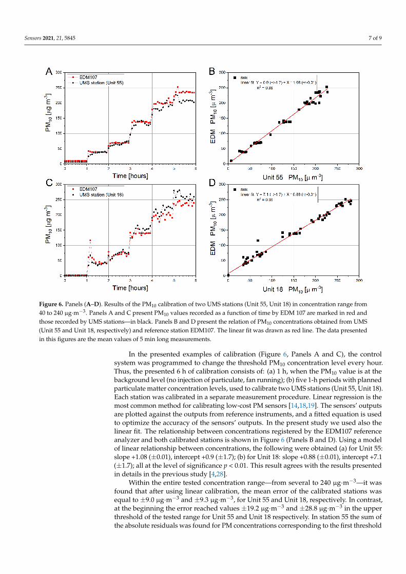
Figure 6. Panels (A–D). Results of the PM10 calibration of two UMS stations (Unit 55, Unit 18) in concentration range from 40 to 240 µg·m−3. Panels A and C present PM10 values recorded as a function of time by EDM 107 are marked in red and those recorded by UMS stations—in black. Panels B and D present the relation of PM10 concentrations obtained from UMS (Unit 55 and Unit 18, respectively) and reference station EDM107. The linear fit was drawn as red line. The data presented in this figures are the mean values of 5 min long measurements.
In the presented examples of calibration (Figure 6, Panels A and C), the control sys-tem was programmed to change the threshold PM10 concentration level every hour. Thus, the presented 6 h of calibration consists of: (a) 1 h, when the PM10 value is at the back-ground level (no injection of particulate, fan running); (b) five 1-h periods with planned particulate matter concentration levels, used to calibrate two UMS stations (Unit 55, Unit 18). Each station was calibrated in a separate measurement procedure. Linear regression is the most common method for calibrating low-cost PM sensors [14,18,19]. The sensors’ outputs are plotted against the outputs from reference instruments, and a fitted equation is used to optimize the accuracy of the sensors’ outputs. In the present study we used also the linear fit. The relationship between concentrations registered by the EDM107 reference analyzer and both calibrated stations is shown in Figure 6 (Panels B and D). Using a model of linear relationship between concentrations, the following were obtained (a) for Unit 55: slope +1.08 (±0.01), intercept +0.9 (±1.7); (b) for Unit 18: slope +0.88 (±0.01), intercept +7.1 (±1.7); all at the level of significance p < 0.01. This result agrees with the results presented in details in the previous study [4,28].
Within the entire tested concentration range—from several to 240 µg·m−3—it was found that after using linear calibration, the mean error of the calibrated stations was equal to ±9.0 µg·m−3 and ±9.3 µg·m−3, for Unit 55 and Unit 18, respectively. In contrast, at
Figure 6. Panels (A–D). Results of the PM10 calibration of two UMS stations (Unit 55, Unit 18) in concentration range from40 to 240 µg·m−3. Panels A and C present PM10 values recorded as a function of time by EDM 107 are marked in red andthose recorded by UMS stations—in black. Panels B and D present the relation of PM10 concentrations obtained from UMS(Unit 55 and Unit 18, respectively) and reference station EDM107. The linear fit was drawn as red line. The data presentedin this figures are the mean values of 5 min long measurements.
In the presented examples of calibration (Figure 6, Panels A and C), the controlsystem was programmed to change the threshold PM10 concentration level every hour.Thus, the presented 6 h of calibration consists of: (a) 1 h, when the PM10 value is at thebackground level (no injection of particulate, fan running); (b) five 1-h periods with plannedparticulate matter concentration levels, used to calibrate two UMS stations (Unit 55, Unit 18).Each station was calibrated in a separate measurement procedure. Linear regression is themost common method for calibrating low-cost PM sensors [14,18,19]. The sensors’ outputsare plotted against the outputs from reference instruments, and a fitted equation is usedto optimize the accuracy of the sensors’ outputs. In the present study we used also thelinear fit. The relationship between concentrations registered by the EDM107 referenceanalyzer and both calibrated stations is shown in Figure 6 (Panels B and D). Using a modelof linear relationship between concentrations, the following were obtained (a) for Unit 55:slope +1.08 (±0.01), intercept +0.9 (±1.7); (b) for Unit 18: slope +0.88 (±0.01), intercept +7.1(±1.7); all at the level of significance p < 0.01. This result agrees with the results presentedin details in the previous study [4,28].
Within the entire tested concentration range—from several to 240 µg·m−3—it wasfound that after using linear calibration, the mean error of the calibrated stations wasequal to ±9.0 µg·m−3 and ±9.3 µg·m−3, for Unit 55 and Unit 18, respectively. In contrast,at the beginning the error reached values ±19.2 µg·m−3 and ±28.8 µg·m−3 in the upperthreshold of the tested range for Unit 55 and Unit 18 respectively. In station 55 the sum ofthe absolute residuals was found for PM concentrations corresponding to the first threshold

Sensors 2021, 21, 5845 8 of 9
(40 µg·m−3) and maximal sum of the absolute residuals was found for PM concentrationscorresponding to the last threshold (240 µg·m−3), where—as for station 18—the minimalsum of the absolute residuals was present at the third PM threshold (140 µg·m−3) andthe maximal sum of absolute residuals was found at the first PM threshold (40 µg·m−3).As presented in Figure 6, Panels A and C, the time responses of the UMS and the EDM arevery similar. Moreover, the EDM reproducibility (Figures 5 and 6) is very similar as well.
It is worth mentioning that the presented calibration system is successfully used tomaintain our continuous air quality measurements within the framework of the scien-tific project known as the Storm&DustNet implemented at the Jagiellonian University inKraków (Poland), as described previously [4].
4. Conclusions
This study presents a simple and low-cost system dedicated for calibration of low-cost suspended particulate matter sensors, with programmed air velocity and known airtemperature and humidity. It allows one to calibrate PM sensors regardless of current fieldconditions using standard solid particles (i.e., standard quartz dust). It should be notedthat this is essential for a system composed of a large number of low-cost sensors.
In our opinion, the presented new calibration system opens the possibility of enhanc-ing the quality of measurements with low-cost PM sensors. This could be achieved byperforming regular calibration procedures that allow the functional state of sensors tobe diagnosed.
In addition, this study examined accuracy of two low-cost UMS stations measuringPM10 within concentration range of up to 240 µg·m–3. The presented final results ofcalibration of both stations (see Figure 6) show that the calibrated readings of both stationsare characterized by similar accuracy of about ±9.0 µg·m–3 within the entire range of PM10concentrations under analysis.
Author Contributions: Conceptualization, Z.N. and J.A.Z.; methodology, Z.N.; software, Z.N.; val-idation, Z.N.; formal analysis, Z.N. and J.A.Z.; investigation, Z.N.; resources, Z.N.; data curation,Z.N.; writing—original draft preparation, Z.N.; writing—review and editing, Z.N. and J.A.Z.; visual-ization, Z.N.; supervision, Z.N. and J.A.Z.; project administration, Z.N.; funding acquisition, Z.N.Both authors have read and agreed to the published version of the manuscript.
Funding: This research was funded by the Jagiellonian University and the APC was funded bythe Faculty of Physics, Astronomy and Applied Computer Science of the Jagiellonian Universityin Kraków.
Conflicts of Interest: The authors declare no conflict of interest.
References1. Kim, K.-H.; Kabir, E.; Kabir, S. A review on the human health impact of airborne particulate matter. Environ. Int. 2015, 74, 136–143.
[CrossRef]2. Chen, L.-J.; Ho, Y.-H.; Lee, H.-C.; Wu, H.-C.; Liu, H.-M.; Hsieh, H.-H.; Huang, Y.-T.; Lung, S.-C.C. An Open Framework for
Participatory PM2.5 Monitoring in Smart Cities. IEEE Access 2017, 5, 14441–14454. [CrossRef]3. Kaliszewski, M.; Włodarski, M.; Młynczak, J.; Kopczynski, K. Comparison of Low-Cost Particulate Matter Sensors for Indoor Air
Monitoring during COVID-19 Lockdown. Sensors 2020, 20, 7290. [CrossRef]4. Nieckarz, Z.; Zoladz, J.A. Low-cost air pollution monitoring system—an opportunity for reducing the health risk associated with
physical activity in polluted air. PeerJ 2020, 8, e10041. [CrossRef]5. Zoladz, J.A.; Nieckarz, Z. Marathon race performance increases the amount of particulate matter deposited in the respiratory
system of runners: An incentive for “clean air marathon runs”. PeerJ 2021, 9, e11562. [CrossRef]6. Pawlak, K.; Nieckarz, Z. The impact of smog on the concentration of particulate matter in the antelope house in the Silesian
zoological garden. PeerJ 2020, 8, e9191. [CrossRef] [PubMed]7. Castell, N.; Dauge, F.R.; Schneider, P.; Vogt, M.; Lerner, U.; Fishbain, B.; Broday, D.; Bartonova, A. Can commercial low-cost sensor
platforms contribute to air quality monitoring and exposure estimates? Environ. Int. 2017, 99, 293–302. [CrossRef] [PubMed]8. Clements, A.L.; Griswold, W.G.; Rs, A.; Johnston, J.E.; Herting, M.M.; Thorson, J.; Collier-Oxandale, A.; Hannigan, M. Low-Cost
Air Quality Monitoring Tools: From Research to Practice (A Workshop Summary). Sensors 2017, 17, 2478. [CrossRef] [PubMed]9. Mei, H.; Han, P.; Wang, Y.; Zeng, N.; Liu, D.; Cai, Q.; Deng, Z.; Wang, Y.; Pan, Y.; Tang, X. Field Evaluation of Low-Cost Particulate
Matter Sensors in Beijing. Sensors 2020, 20, 4381. [CrossRef]

Sensors 2021, 21, 5845 9 of 9
10. Zusman, M.; Schumacher, C.S.; Gassett, A.J.; Spalt, E.W.; Austin, E.; Larson, T.V.; Carvlin, G.; Seto, E.; Kaufman, J.D.; Sheppard, L.Calibration of low-cost particulate matter sensors: Model development for a multi-city epidemiological study. Environ. Int. 2019,134, 105329. [CrossRef] [PubMed]
11. Lewis, A.; Edwards, P. Validate personal air-pollution sensors. Nature 2016, 535, 29–31. [CrossRef]12. Chen, L.-J.; Ho, Y.-H.; Hsieh, H.-H.; Huang, S.-T.; Lee, H.-C.; Mahajan, S. ADF: An Anomaly Detection Framework for Large-Scale
PM2.5 Sensing Systems. IEEE Internet Things J. 2017, 5, 559–570. [CrossRef]13. Jo, S.; Lee, S.; Leem, Y. Temporal Changes in Air Quality According to Land-Use Using Real Time Big Data from Smart Sensors in
Korea. Sensors 2020, 20, 6374. [CrossRef] [PubMed]14. Li, J.; Mattewal, S.K.; Patel, S.; Biswas, P. Evaluation of Nine Low-cost-sensor-based Particulate Matter Monitors. Aerosol Air Qual.
Res. 2020, 20, 254–270. [CrossRef]15. Bokwa, A. Environmental Impacts of long-term air pollution changes in Kraków, Poland. Pol. J. Environ. Stud. 2008, 17, 673–686.16. Kwak, H.-Y.; Ko, J.; Lee, S.; Joh, C.-H. Identifying the correlation between rainfall, traffic flow performance and air pollution
concentration in Seoul using a path analysis. Transp. Res. Procedia 2017, 25, 3552–3563. [CrossRef]17. Manikonda, A.; Zikova, N.; Hopke, P.K.; Ferro, A.R. Laboratory assessment of low-cost PM monitors. J. Aerosol Sci. 2016, 102,
29–40. [CrossRef]18. Kelly, K.; Whitaker, J.; Petty, A.; Widmer, C.; Dybwad, A.; Sleeth, D.; Martin, R.; Butterfield, A. Ambient and laboratory evaluation
of a low-cost particulate matter sensor. Environ. Pollut. 2017, 221, 491–500. [CrossRef]19. Badura, M.; Batog, P.; Drzeniecka-Osiadacz, A.; Modzel, P. Evaluation of Low-Cost Sensors for Ambient PM2.5 Monitoring.
J. Sensors 2018, 2018, 5096540. [CrossRef]20. Papapostolou, V.; Zhang, H.; Feenstra, B.J.; Polidori, A. Development of an environmental chamber for evaluating the performance
of low-cost air quality sensors under controlled conditions. Atmos. Environ. 2017, 171, 82–90. [CrossRef]21. Wang, Y.; Li, J.; Jing, H.; Zhang, Q.; Jiang, J.; Biswas, P. Laboratory Evaluation and Calibration of Three Low-Cost Particle Sensors
for Particulate Matter Measurement. Aerosol Sci. Technol. 2015, 49, 1063–1077. [CrossRef]22. Omidvarborna, H.; Kumar, P.; Tiwari, A. ‘Envilution™’ chamber for performance evaluation of low-cost sensors. Atmos. Environ.
2020, 223, 117264. [CrossRef]23. Spinelle, L.; Gerboles, M.; Aleixandre, M. Report of Laboratory and In-Situ Validation of Micro-Sensor for Monitoring Ambient Air:
Ozone Micro-Sensor Alphasense, Model B4-O3 Sensor; JRC90463; Publications Office of the European Union: Luxembourg, 2014.[CrossRef]
24. Kotas, P.; Twardosz, R.; Nieckarz, Z. Variability of air mass occurrence in southern Poland (1951–2010). Theor. Appl. Clim. 2013,114, 615–623. [CrossRef]
25. Huang, Q.; Cai, X.; Wang, J.; Song, Y.; Zhu, T. Climatological study of a new air stagnation index (ASI) for China and itsrelationship with air pollution. Atmos. Chem. Phys. Discuss. 2018, 1, 39. [CrossRef]
26. Celik, A.N.; Makkawi, A.; Muneer, T. Critical evaluation of wind speed frequency distribution functions. J. Renew. Sustain. Energy2010, 2, 13102. [CrossRef]
27. Bridgwater, J. Mixing and Segregation Mechanisms in Particle Flow. In Granular Matter; Mehta, A., Ed.; Springer: New York, NY,USA, 1994.
28. Rogulski, M. Low-cost PM monitors as an opportunity to increase the spatiotemporal resolution of measurements of air quality.Energy Procedia 2017, 128, 437–444. [CrossRef]