new hybrid multi-criteria decision-making dematel-mairca

Full Terms & Conditions of access and use can be found athttp://www.tandfonline.com/action/journalInformation?journalCode=rero20

Economic Research-Ekonomska Istraživanja

ISSN: 1331-677X (Print) 1848-9664 (Online) Journal homepage: http://www.tandfonline.com/loi/rero20

New hybrid multi-criteria decision-makingDEMATEL-MAIRCA model: sustainable selectionof a location for the development of multimodallogistics centre

Dragan S. Pamucar, Snezana Pejcic Tarle & Tanja Parezanovic

To cite this article: Dragan S. Pamucar, Snezana Pejcic Tarle & Tanja Parezanovic (2018) Newhybrid multi-criteria decision-making DEMATEL-MAIRCA model: sustainable selection of a locationfor the development of multimodal logistics centre, Economic Research-Ekonomska Istraživanja,31:1, 1641-1665, DOI: 10.1080/1331677X.2018.1506706

To link to this article: https://doi.org/10.1080/1331677X.2018.1506706

© 2018 The Author(s). Published by InformaUK Limited, trading as Taylor & FrancisGroup.

Published online: 15 Nov 2018.

Submit your article to this journal

Article views: 37

View Crossmark data

http://www.tandfonline.com/action/journalInformation?journalCode=rero20

http://www.tandfonline.com/loi/rero20

http://www.tandfonline.com/action/showCitFormats?doi=10.1080/1331677X.2018.1506706

https://doi.org/10.1080/1331677X.2018.1506706

http://www.tandfonline.com/action/authorSubmission?journalCode=rero20&show=instructions

http://www.tandfonline.com/action/authorSubmission?journalCode=rero20&show=instructions

http://crossmark.crossref.org/dialog/?doi=10.1080/1331677X.2018.1506706&domain=pdf&date_stamp=2018-11-15

http://crossmark.crossref.org/dialog/?doi=10.1080/1331677X.2018.1506706&domain=pdf&date_stamp=2018-11-15

New hybrid multi-criteria decision-making DEMATEL-MAIRCA model: sustainable selection of a location for thedevelopment of multimodal logistics centre

Dragan S. Pamucara, Snezana Pejcic Tarleb and Tanja Parezanovicb

aDepartment of Logistics, University of Defence in Belgrade, Belgrade, Serbia; bFaculty of Transportand Traffic Engineering, University of Belgrade, Belgrade, Serbia

ABSTRACTThe paper describes the application of a new multi-criteria deci-sion-making (MCDM) model, MultiAtributive Ideal-Real ComparativeAnalysis (MAIRCA), used to select a location for the development ofa multimodal logistics centre by the Danube River. The MAIRCAmethod is based on the comparison of theoretical and empiricalalternative ratings. Relying on theoretical and empirical ratings thegap (distance) between the empirical and ideal alternative isdefined. To determine the weight coefficients of the criteria, theDEMATEL method was applied. In this paper, through a sensitivityanalysis, the results of MAIRCA and other MCDM methods –MOORA, TOPSIS, ELECTRE, COPRAS and PROMETHEE – were com-pared. The analysis showed that a smaller or bigger instability inalternative rankings appears in MOORA, TOPSIS, ELECTRE andCOPRAS. On the other hand, the analysis showed that MAIRCA andPROMETHEE offer consistent solutions and have a stable and well-structured analytical framework for ranking the alternatives. By pre-senting a new method MCDM expands the theoretical frameworkof expertise in the field of MCDM. This enables the analysis of prac-tical problems with new methodology and creates a basis for fur-ther theoretical and practical upgrade.

ARTICLE HISTORYReceived 11 June 2016Accepted 24 May 2017

KEYWORDSMAIRCA; DEMATEL; locationplanning; multi-criteriadecision-making

JEL CLASSIFICATIONCODESC61; C67; L1; L16

1. Introduction

The logistics centre (LC) is a unique technological, spatial, organisational and eco-nomic entity bringing together different providers and users of logistics services. Theoptimal LC location reduces transportation costs, improves business performance,competitiveness and profitability. The objective is to identify the location that oper-ates at minimal cost and maximum efficiency, while meeting operational and strategicrequirements.

LC location selection is the process in which one of the possible alternatives ischosen. A large number of heterogeneous location factors make the location probleman interdisciplinary one, requiring a complex selection procedure. There are many

CONTACT Dragan Pamucar [email protected]� 2018 The Author(s). Published by Informa UK Limited, trading as Taylor & Francis Group.This is an Open Access article distributed under the terms of the Creative Commons Attribution License (http://creativecommons.org/licenses/by/4.0/), which permits unrestricted use, distribution, and reproduction in any medium, provided the original work isproperly cited.

ECONOMIC RESEARCH-EKONOMSKA ISTRA�ZIVANJA2018, VOL. 31, NO. 1, 1641–1665https://doi.org/10.1080/1331677X.2018.1506706

http://crossmark.crossref.org/dialog/?doi=10.1080/1331677X.2018.1506706&domain=pdf

http://creativecommons.org/licenses/by/4.0/

http://creativecommons.org/licenses/by/4.0/

https://doi.org./10.1080/1331677X.2018.1506706

http://www.tandfonline.com

methodologies and procedures available in this area (Badi and Ballem, 2018;Milosavljevic, Bursa�c, & Tri�ckovi�c, 2018). The selection of the location for LC devel-opment can be considered to be a special case within a general facility location prob-lem. The facility location problem usually involves a set of locations (alternatives)which are evaluated against a set of weighed criteria independent from each other.

There are many ways to solve facility location problems including the dual-basedalgorithm proposed by Erlenkotter (1978). Several improved versions of this ideahave been proposed to solve the problem (Jan�a�cek & Buzna, 2008; Ji, Tang, Li, Yang,

Gather the opinion of experts and calculate

the average matrix Z

Calculate the normalized initial direction

matrix D

Derive the total relation matrix T

Calculate the sums of the rows and columns

of matrix T

Determine the weight coefficients of the

criteria

Normalization of the weight coefficients of

the criteria

Formation of the initial decision matrix

(evaluation of the alternatives by criteria)

Definition of preferences for alternatives

(PAi)

Calculation of the elements of theoretical

ratings matrix (Tp)

Calculation of the elements of the total gap

matrix (G)

Calculation of the elements of real ratings

matrix (Tr)

The selection of the optimal alternative

PhaseIoftheDEMATELmethod

I dentificationofthecriteriaandcalculationoftheirweight

PhaseIIoftheMAIRCAmethod

Evaluationandselectionoftheoptimalalternative

Definition of the total gap by alternatives

(Qi)

Calculation of the value of criteria

functions and ranking the alternatives

Figure 1. Phases of the hybrid DEMATEL–MAIRCA model. Source: Provided by authors.

1642 D. S. PAMUCAR ET AL.

& Liao, 2016; Mladenovi�c, Brimberg, Hansen, & Moreno-P�erez, 2007). Other popularmethods include local search (Brimberg, Drezner, Mladenovi�c, & Salhi, 2014), tabusearch (Wang, Li, Yuan, Ye, & Wang, 2016b), neighbourhood search (Qazi, Lam,Xiao, Ouyang, & Yin, 2016), etc.

Many classical and heuristic methods have been proposed to solve a location prob-lem, like linear, non-linear programming, simplex algorithm, lagrangian relaxation,branch and cut methods, branch and bound (Liu, Wang, & Jin, 2016c), artificialneural network (Wan, Huang, & Li, 2007), generic algorithms, expert systems, multi-agent systems, hybrid algorithms (Han, Li, Wang, & Shi, 2016; Xu, Law, Chen, &Tang, 2016a; Zare et al., 2013) and so on.

There are different studies associated with location selection decisions that havebeen commonly carried out using MCDM techniques, such as distribution centreselection with weighted fuzzy factor rating system (Ou & Chou, 2009; Xu, Dong,Zhang, & Xu, 2016b; Zhang, Xie, & Wang, 2016), location problem with fuzzy-AHP(Petrovi�c and Kankara�s, 2018), location problem with MOORA and COPRAS meth-ods (Kracka, Brauers, & Zavadskas, 2010; Rezaeiniya, Zolfani, & Zavadskas, 2012),intermodal freight hub location decision with multi-objective evaluation model(Sirikijpanichkul & Ferreira, 2006; Yang, Sun, Deng, Zhang, & Liao, 2016), selectionof LC location with fuzzy TOPSIS based on entropy weight (Chen & Liu, 2006),deep-water port location with AHP and fuzzy ratio assessment methods (Zavadskas,Turskis, & Bago�cius, 2015), construction site selection with fuzzy AHP and weightedaggregated sum-product assessment method (Turskis, Zavadskas, Antucheviciene, &Kosareva, 2015), facility location selection with AHP and ELECTRE (Yang & Lee,1997), port selection with AHP and PROMETHEE (Zecevic, 2006), reverse logisticslocation selection with MOORA (Kannan, Nooral Haq, & Sasikumar, 2008) andselecting a site for a logistical centre on factor and methods (Chen & Liu, 2006).

The research listed above singles out MOORA, COPRAS, TOPSIS, ELECTRE andPROMETHEE as most frequently used in the LC location selection process. In thispaper the MAIRCA method was used to select the LC location. The next step was tocompare the MAIRCA results with the results obtained when MOORA, COPRAS,TOPSIS, ELECTRE and PROMETHEE methods were applied. Based on a subsequentsensitivity analysis, these methods were assessed objectively and the method maintain-ing the consistency of results selected. Two consistency criteria were defined to gaugethe sensitivity of the results: (1) the consistency of results depending on a varyingvalue scale and (2) the consistency of results depending on the formulation of criteria,if the same criteria can be presented in two normatively equivalent ways. The LC siteselection showed that some of the MCDM methods used did not meet one of the cri-teria or, very often, both of them.

The paper presents a MCDM hybrid model (Figure 1), incorporating a fuzzyDEMATEL method (Dalalah, Hayajneh, & Batieha, 2011) and a new MCDM method,MAIRCA, developed by Professor Dragan Pamu�car in the Logistics Research Centreat the Belgrade-based Defence University. The modified fuzzy DEMATEL methodwas used to estimate the criteria and define the criterion weights.

Having defined the weights of the criteria based on the MAIRCA method, theoptimal LC location was selected.

ECONOMIC RESEARCH-EKONOMSKA ISTRA�ZIVANJA 1643

2. Setting up the hybrid DEMATEL–MAIRCA model

The causal relationship among the criteria is determined by using a modified fuzzyDEMATEL method. The modified fuzzy DEMATEL method which is used in thispaper is adapted from the studies of Dalalah et al. (2011).

The problem is formally presented by choosing one of the m options (alternatives),Ai; i ¼ 1; 2; :::;m, which we evaluate and compare with each other based on the n cri-teria (Xj; j ¼ 1; 2; :::; n), the values of which are known to us. The alternatives aredescribed by the vectors xij, where xij is the value of the i-alternative by the j-criter-ion. As the impact of the criteria on the final ranking of alternatives varies, each cri-terion is assigned a weight ratio wj; j ¼ 1; 2; :::; n (where

Pnj¼1 wj ¼ 1), reflecting its

relative significance in evaluating the alternatives. In this step of the proposed model,the relationship among the criteria is determined by using the modified fuzzyDEMATEL method. The implementation process for the modified fuzzy DEMATELmethod is described in the next section.

Step 1 serves to collect expert scores and calculate the average matrix eZ . A groupof m experts and n factors are used in this step. Each expert is to determine the influ-ence level of factor i on factor j. Comparative analysis of the ith and jth factors’ pairby kth expert is labelled with zij

e, where i ¼ 1,… ,n; j¼ 1,… ,n; e¼ 1,… ,m.For each expert, a n� n non-negative matrix is constructed (n represents the num-

ber of criteria) as eZe ¼ ½ezeij�, where e is the expert number of participating in evalu-ation process with 1 � e � m. Thus, eZ1

; eZ2; :::; eZm

are the matrices from m experts.In this method, the effects of the criteria on each other are expressed in terms of lin-guistic expressions. The experts list the pairwise comparisons based on a fuzzifiedscale, where the linguistic expressions are described by triangular fuzzy numbersezeij¼ ðzðlÞ

ij;e; zðsÞ

ij;e; zðrÞ

ij;eÞ; e ¼ 1; 2; :::;m, where e is the expert number, and m represents a

total number of experts. The aggregation of expert opinions results in the final matrixeZ ¼ ½ezij�.Equations (1), (2) and (3) are the formulas for obtaining the matrix eZ elements:

z lð Þij;e

¼ minM

z lð Þij;e

n o; M ¼ 1; 2; :::; e; :::;mf g (1)

z sð Þij;e

¼ 1m

Xmk¼1

z sð Þij;k

(2)

z rð Þij;e

¼ maxM

z rð Þij;e

n o; M ¼ 1; 2; :::; e; :::;mf g (3)

where zðlÞij;e, zðsÞ

ij;eand zðrÞ

ij;erepresent a preference by e-expert, M is a set of experts tak-

ing part in the research, e is the expert score, and m a total number of experts.Having calculated the elements of the matrix eZ , the next step defines the elements

of the normalised initial direct-relation matrix eD ¼ ½edij�. The elements of the matrixeD (Eq. 4) are calculated based on formulas (5) and (6).


eD ¼ed11

ed12 ::: ed1ned21ed22 ::: ed2n

::: ::: ::: :::edn1edn2 ::: ednn

2666437775 (4)

The matrix eD elements are obtained by summing up the elements of the averagematrix eZ by rows. Having applied Eq. (6), the maximum element eR is identifiedamong the summed elements. By simple normalisation, Eq. (5), each element of thematrix eZ is divided by the result of formula (6).

edij ¼ezijeR ¼

z lð Þij

r lð Þ ;z sð Þij

r sð Þ ;z rð Þij

r rð Þ

!(5)

eR ¼ maxXn

j¼1ezij� �

¼ r lð Þ; r sð Þ; r rð Þ� �

(6)

where n represents the total number of criteria.In the next step the elements of the total relation matrix eTare calculated.

Therefore, the total-relation fuzzy matrix eT can be acquired by calculating the follow-ing term (Dalalah et al., 2011):

eT ¼ limw!/

eD þ eD2 þ :::þ eDw� �

¼ eD I � eDð Þ�1(7)

Based on the above, the total-relation matrix for the criteria (eT ) can be presentedas:

eT ¼et11 et12 ::: et1net21 et22 ::: et2n::: ::: ::: :::etn1 etn2 ::: etnn

2666437775 (8)

where et11 ¼ ðtðlÞij; tðsÞ

ij; tðrÞ

ijÞ is the overall influence rating by a decision-maker for

each criterion i against criterion j.In the last step of the DEMATEL method, summing by rows and columns of the

matrix elements eT is completed. The sum of rows and the sum of columns of thesub-matrices T1, T2 and T3 denoted by the fuzzy numbers eDi and eRi, respectively,can be obtained through Eqs. (9) and (10), respectively:

eDi ¼Xn

i¼1et ij; i ¼ 1; 2; :::; n (9)

eRj ¼Xn

j¼1et ij; j ¼ 1; 2; :::; n (10)

where n is the number of criteria.


Based on the values obtained from formulas (9) and (10), the criterion weights arecalculated. The criterion weights are calculated using formulas (11) and (12):

eWi ¼ eDi þ eRj

� �2þ eDi � eRj

� �2� �1=2(11)

By formula (11) the fuzzy value of weight coefficients W�

i ¼ ðWðlÞi ;WðsÞ

i ;WðrÞi Þis

obtained and it has to be normalized by formula (12). To simplify the normalisationof weight coefficients, defuzzification of the value of weight coefficients from the for-mula (11) is preformed prior to normalisation. Defuzzification of weight coefficientsis carried out by implementing the formula:

W ¼ W rð Þ �W lð Þ� �

þ W sð Þ �W lð Þ� ��

� 1=3þW lð Þ:

Weight coefficient values after defuzzification are normalised by formula (12):

wi ¼ WiPni¼1 Wi

(12)

where wi represents the final criteria weights to be used in the decision making pro-cess (Dalalah et al., 2011).

Defining the criterion weights creates conditions for presenting a mathematicalformulation of the MAIRCA model. The basic MAIRCA set up is to define the gapbetween ideal and empirical ratings. Summing the gap by each criterion generates thetotal gap for each alternative observed. Ranking the alternatives comes at the end ofthe process, where the best-ranked alternative is the one with the lowest gap value.The alternative with the lowest total gap value is the alternative, by most of the crite-ria, with the values closest to the ideal ratings (the ideal criteria values).

The MAIRCA method is carried out in six steps.Step 1. Formulation of the initial decision-making matrix (X). The initial decision-

making matrix (13) determines the criteria values (xij; i ¼ 1; 2; :::n; j ¼ 1; 2; :::m) foreach alternative observed.

X ¼A1

A2

:::Am

C1 C2 ::: Cn

x11 x12 ::: x1nx21 x22 x2n::: ::: ::: :::xm1 x22 ::: xmn

26643775 (13)

The criteria from the matrix (13) can be quantitative (measurable) and qualitative(descriptive). The quantitative criteria values in the matrix (13) are obtained by quan-tification of real indicators which present the criteria. The qualitative criteria valuesare determined by decision-maker’s preferences or, in the case of a large number ofexperts, by aggregating the experts’ opinions.

Step 2. Defining preferences for the choice of alternatives PAi . While selecting thealternatives, the decision-maker (DM) is neutral, meaning there’s no preference for


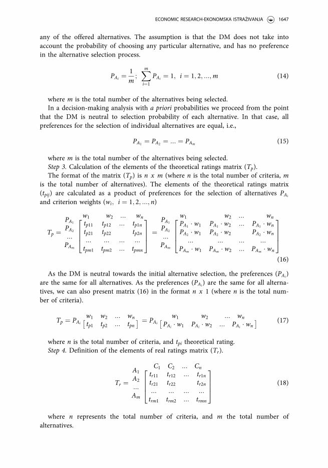
any of the offered alternatives. The assumption is that the DM does not take intoaccount the probability of choosing any particular alternative, and has no preferencein the alternative selection process.

PAi ¼1m;Xmi¼1

PAi ¼ 1; i ¼ 1; 2; :::;m (14)

where m is the total number of the alternatives being selected.In a decision-making analysis with a priori probabilities we proceed from the point

that the DM is neutral to selection probability of each alternative. In that case, allpreferences for the selection of individual alternatives are equal, i.e.,

PA1 ¼ PA2 ¼ ::: ¼ PAm (15)

where m is the total number of the alternatives being selected.Step 3. Calculation of the elements of the theoretical ratings matrix (Tp).The format of the matrix (Tp) is n x m (where n is the total number of criteria, m

is the total number of alternatives). The elements of the theoretical ratings matrix(tpij) are calculated as a product of preferences for the selection of alternatives PAi

and criterion weights (wi; i ¼ 1; 2; :::; n)

Tp ¼PA1

PA2

:::PAm

w1 w2 ::: wntp11 tp12 ::: tp1ntp21 tp22 tp2n::: ::: ::: :::tpm1 tpm2 ::: tpmn

26643775 ¼

PA1

PA2

:::PAm

w1 w2 ::: wn

PA1 � w1 PA1 � w2 ::: PA1 � wn

PA2 � w1 PA2 � w2 PA2 � wn

::: ::: ::: :::PAm � w1 PAm � w2 ::: PAm � wn

26643775(16)

As the DM is neutral towards the initial alternative selection, the preferences (PAi)are the same for all alternatives. As the preferences (PAi) are the same for all alterna-tives, we can also present matrix (16) in the format n x 1 (where n is the total num-ber of criteria).

Tp ¼ PAi

w1 w2 ::: wn

tp1 tp2 ::: tpn� ¼ PAi

w1 w2 ::: wn

PAi � w1 PAi � w2 ::: PAi � wn� (17)

where n is the total number of criteria, and tpi theoretical rating.Step 4. Definition of the elements of real ratings matrix (Tr).

Tr ¼A1

A2

:::Am

C1 C2 ::: Cn

tr11 tr12 ::: tr1ntr21 tr22 tr2n::: ::: ::: :::trm1 trm2 ::: trmn

26643775 (18)

where n represents the total number of criteria, and m the total number ofalternatives.


In calculation of the elements of the real ratings matrix (Tr) the elements of thetheoretical ratings matrix (Tp) are multiplied by the elements of the initial decision-making matrix (X) using the following formulas:

� For the benefit type criteria (preferred higher criteria value):

trij ¼ tpij �xij�x�ixþi � x�i

�(19)

� For the cost type criteria (preferred lower criteria value):

trij ¼ tpij �xij�xþix�i � xþi

!(20)

where xij, xþi and x�i represent the elements of the initial decision-making matrix(X), and xþi and x�i are defined as: xþi ¼ maxðx1; x2; :::; xmÞ, representing the max-imum values of the observed criterion by alternatives; x�i ¼ minðx1; x2; :::; xmÞ, repre-senting the minimum values of the observed criterion by alternatives.

Step 5. The calculation of the total gap matrix (G). The elements of the G matrixare obtained as a difference (gap) between the theoretical (tpij) and real ratings (trij),i.e., a difference between the theoretical ratings matrix (Tp) and the real ratingsmatrix (Tr)

G ¼ Tp�Tr ¼g11 g12 ::: g1ng21 g22 ::: g2n::: ::: ::: :::gm1 gm2 ::: gmn

26643775 ¼

tp11�tr11 tp12�tr12 ::: tp1n�tr1ntp21�tr21 tp22�tr22 ::: tp2n�tr2n

::: ::: ::: :::tpm1�trm1 tpm2�trm2 ::: tpmn�trmn

26643775(21)

where n represents the total number of criteria, m is the total number of the alter-natives being selected.

The gap gij takes the values from the interval gij 2 ½0;1Þ, by Eq. (22):

gij ¼ tpij�trij (22)

The preferable option is that gij gravitates towards zero (gij ! 0), because we arechoosing the alterative with the smallest difference between theoretical ratings (tpij)and real ratings (trij). If for criterion Ci the alternative Ai has a theoretical ratingvalue equal to the real rating value (tpij ¼ trij), the gap for alternative Ai, by criterionCi, is gij ¼ 0. In other words, by criterion Ci, alternative Ai is the best (ideal) alterna-tive (Aþ

i ).If by criterion Ci alternative Ai has the value of theoretical ratings tpij, and the

value of real ratings trij ¼ 0, the gap for alternative Ai, by criterion Ci, is gij ¼ tpij. Inother words, alternative Ai is the worst (anti-ideal) alternative (A�

i ) by criterion Ci.


Step 6. The calculation of the final values of criteria functions (Qi) by alternatives.The values of criteria functions are obtained by summing the gap (gij) by alternatives,that is, by summing the elements of matrix (G) by columns, Eq. (23):

Qi ¼Xnj¼1

gij; i ¼ 1; 2; :::;m (23)

where n is the total number of criteria, and m is the total number of the alterna-tives being selected.

3. Selection of a location for the development of multimodal logisticscentre based on the DEMATEL–MAIRCA method

This paper has focused on the selection of a multimodal LC location, linking threemodes of transportation (river, railway and road transportation). As an example, eightpotential locations for the development of the multimodal LC have been consideredin Serbia, along the Danube River (Transportation Corridor VII). Having analysedthe above-mentioned literature, the characteristics of the multimodal LC and thelogistic trends, the authors identified 11 criteria against which to select the LC loca-tion: Connectivity to Multimodal Transport (CMT), Estimate of InfrastructureDevelopment (EID), Environmental Impact (EI), Conformity With Spatial PlanningPolicy and Economic Growth Strategy (CSPPEGS), Gravitating Intermodal TransportUnits (GITU), Reload LC Capacity (RC), Area Available for LC Development andCapacity Expansion (AADCE), Distance Between the User and the LC (DBULC),Transportation Safety (TS), Length of the Railway Reload Front (RRF), and EstimatedQuality of Transportation Access to Internal Transport (EQTAIT).

A total of eight locations along the Danube River were discussed for the LC devel-opment. Eight experts took part in the research, defining the weights of the criteriabased on the DEMATEL method.

In Step 1 of the DEMATEL method, a fuzzy scale (Camparo, 2013; Li, 2013),Table 1, is used to evaluate the criteria.

The collected questionnaires produced a total of eight average matriceseZ ¼ ½ezij�Ci�Ci. The expert opinions were aggregated using Eqs. (1), (2) and (3). After

the aggregation of expert opinions, the unique average matrix eZ (Table 2)was obtained.

The elements of the initial direct-relation matrix eD are defined using Eq. (5). Theelements of matrix eD are normalised by dividing each element of the matrix eZ by thevalue eR obtained using formula (6).

Table 1. Fuzzy scal.NO. LINGUISTIC TERMS TRIANGULAR FUZZY NUMBERS

1. Very high influence (VH) (4.50, 5.00, 5.00)2. High influence (H) (2.50, 3.50, 4.50)3. Low influence (L) (1.50, 2.50, 3.50)4. Very low influence (VL) (0.00, 1.50, 2.50)5. No influence (No) (0.00, 0.00, 1.50)

Source: Vasiljevic et al, (2018).


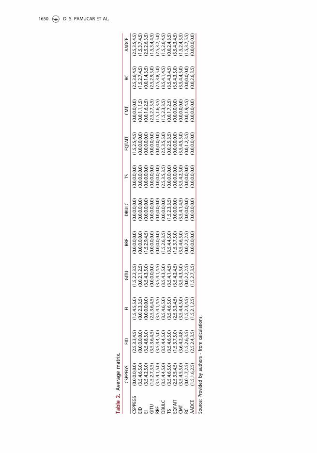
Table2.

Averagematrix.

CSPPEG

SEID

EIGITU

RRF

DBU

LCTS

EQTA

ITCM

TRC

AADCE

CSPPEG

S(0.0,0.0,0.0)

(2.5,3.3,4.5)

(1.5,4.5,5.0)

(1.5,2.2,3.5)

(0.0,0.0,0.0)

(0.0,0.0,0.0)

(0.0,0.0,0.0)

(1.5,2.5,4.5)

(0.0,0.0,0.0)

(2.5,3.6,4.5)

(2.5,3.5,4.5)

EID

(3.5,4.6,5.0)

(0.0,0.0,0.0)

(0.0,2.3,3.5)

(0.0,2.1,2.5)

(0.0,0.0,0.0)

(0.0,0.0,0.0)

(0.0,0.0,0.0)

(0.0,0.0,0.0)

(0.0,1.1,1.5)

(1.5,2.7,4.5)

(1.5,3.7,4.5)

EI(3.5,4.2,5.0)

(3.5,4.8,5.0)

(0.0,0.0,0.0)

(3.5,4.3,5.0)

(1.5,2.9,4.5)

(0.0,0.0,0.0)

(0.0,0.0,0.0)

(0.0,0.0,0.0)

(0.0,1.6,2.5)

(0.0,1.4,3.5)

(2.5,2.6,3.5)

GITU

(1.5,2.7,3.5)

(3.5,3.6,4.5)

(2.5,3.6,4.5)

(0.0,0.0,0.0)

(0.0,0.0,0.0)

(0.0,0.0,0.0)

(0.0,0.0,0.0)

(0.0,0.0,0.0)

(2.5,2.7,3.5)

(2.5,2.9,5.0)

(1.5,3.4,4.5)

RRF

(3.5,4.1,5.0)

(3.5,4.4,5.0)

(3.5,4.1,4.5)

(3.5,4.1,4.5)

(0.0,0.0,0.0)

(0.0,0.0,0.0)

(0.0,0.0,0.0)

(0.0,0.0,0.0)

(1.5,1.6,3.5)

(2.5,3.8,5.0)

(2.5,3.7,5.0)

DBU

LC(3.5,4.4,5.0)

(3.5,4.4,5.0)

(3.5,4.6,5.0)

(3.5,4.3,5.0)

(1.5,2.6,3.5)

(0.0,0.0,0.0)

(2.5,3.5,3.5)

(2.5,3.5,5.0)

(1.5,2.3,3.5)

(3.5,4.1,4.5)

(1.5,2.6,4.5)

TS(3.5,4.6,5.0)

(3.5,4.6,5.0)

(3.5,4.6,5.0)

(3.5,4.1,4.5)

(3.5,4.4,5.0)

(1.5,2.3,3.5)

(0.0,0.0,0.0)

(0.0,2.5,3.5)

(0.0,1.7,2.5)

(3.5,4.3,4.5)

(0.0,2.4,3.5)

EQTA

IT(2.5,3.5,4.5)

(1.5,3.7,5.0)

(2.5,3.3,4.5)

(3.5,4.2,4.5)

(1.5,3.7,5.0)

(0.0,0.0,0.0)

(0.0,0.0,0.0)

(0.0,0.0,0.0)

(0.0,0.0,0.0)

(3.5,4.3,5.0)

(3.5,4.3,4.5)

CMT

(3.5,4.5,5.0)

(3.6,4.2,4.8)

(3.5,4.4,5.0)

(3.5,4.3,5.0)

(3.5,4.6,5.0)

(3.5,4.1,4.5)

(3.5,4.2,5.0)

(3.5,4.5,5.0)

(0.0,0.0,0.0)

(3.5,4.4,5.0)

(1.5,2.4,3.5)

RC(0.0,1.7,2.5)

(1.5,2.6,3.5)

(1.5,2.3,4.5)

(0.0,2.2,2.5)

(0.0,2.2,2.5)

(0.0,0.0,0.0)

(0.0,0.0,0.0)

(0.0,1.2,3.5)

(0.0,1.9,4.5)

(0.0,0.0,0.0)

(1.5,3.7,5.5)

AADCE

(1.5,1.6,2.5)

(2.5,2.4,3.5)

(1.5,2.1,2.5)

(1.5,2.7,3.5)

(0.0,0.0,0.0)

(0.0,0.0,0.0)

(0.0,0.0,0.0)

(0.0,0.0,0.0)

(0.0,0.0,0.0)

(0.0,2.6,3.5)

(0.0,0.0,0.0)

Source:P

rovidedby

authors-from

calculations.


Equation (7) produces the elements of the total-relation matrix (eT). The elementsof matrix eT (Table 3) are summed by rows (eGi) and columns (eRi) using formulas (9)and (10), respectively. Based on the sum of values by rows and columns, formulas(11) and (12) give us the criterion weights. Equation (24) defuzzifies the fuzzy num-bers obtained from Eqs. (9), (10), (11) and (12).

A ¼ a rð Þ � a lð Þ� �

þ a sð Þ � a lð Þ� ��

� 1=3þ a lð Þ (24)

where aðlÞ and aðrÞrepresent the left and right limit of the fuzzy number, respect-ively, and aðmÞ is the value at which the triangular function reaches the maximum.

Table 4 presents the summed values of the matrix T by rows (Di) and columns(Ri) and the criterion weights (wi).

After the calculation of criterion weights (wi), the alternatives are evaluated(Table 6) and selected based on the MAIRCA method. To evaluate the alternatives bythe qualitative criteria, a fuzzy scale was used (Camparo, 2013), Table 5.

Table 4. Criterion weights (wi).Di Ri Di þ Ri Di�Ri Wi wi

CSPPEGS 0.80 1.79 2.60 –0.99 2.78 0.097EID 0.70 2.00 2.69 –1.30 2.99 0.105EI 0.93 1.82 2.75 –0.89 2.89 0.101GITU 0.77 1.74 2.51 –0.97 2.69 0.094RRF 1.12 0.90 2.02 0.22 2.03 0.071DBULC 1.76 0.27 2.02 1.49 2.51 0.088TS 1.66 0.30 1.97 1.36 2.39 0.084EQTAIT 1.09 0.66 1.75 0.43 1.80 0.063CMT 2.08 0.72 2.80 1.36 3.11 0.109RC 0.77 1.72 2.49 –0.94 2.67 0.094AADCE 0.50 1.81 2.32 –1.31 2.66 0.093

Source: Provided by authors - from calculations.

Table 3. Defuzzified total-relation matrix (T).CSPPEGS EID EI GITU RRF DBULC TS EQTAIT CMT RC AADCE

CSPPEGS 0.069 0.158 0.170 0.124 0.029 0.003 0.003 0.073 0.028 0.144 0.157EID 0.161 0.066 0.120 0.115 0.024 0.007 0.007 0.022 0.061 0.112 0.147EI 0.181 0.187 0.083 0.177 0.083 0.008 0.008 0.024 0.070 0.109 0.139GITU 0.125 0.157 0.152 0.066 0.029 0.010 0.010 0.023 0.083 0.116 0.152RRF 0.197 0.205 0.199 0.194 0.035 0.009 0.009 0.028 0.077 0.167 0.183DBULC 0.252 0.262 0.255 0.248 0.127 0.019 0.104 0.135 0.115 0.238 0.206TS 0.244 0.254 0.247 0.240 0.164 0.071 0.017 0.102 0.095 0.230 0.199EQTAIT 0.176 0.185 0.180 0.175 0.119 0.004 0.005 0.023 0.038 0.185 0.202CMT 0.281 0.292 0.284 0.277 0.187 0.125 0.129 0.164 0.070 0.265 0.232RC 0.108 0.131 0.127 0.125 0.085 0.008 0.008 0.057 0.064 0.062 0.155AADCE 0.077 0.099 0.096 0.094 0.014 0.002 0.002 0.010 0.018 0.090 0.042


Table 5. Fuzzy scale for the evaluation of alternatives.NO. LINGUISTIC TERMS LINGUISTIC VALUES

1. Very good (VG) (4.5,5,5)2. Good (G) (3.5,4,4.5)3. Fair (F) (2.5,3,3.5)4. Poor (P) (1.5,2,2.5)5. Very poor (VP) (1,1,1)

Source: Pamucar and Cirovic (2015).


In Table 6 the criteria are categorised; max stands for the benefit-type criteria(higher values are preferable), and min stands for the cost-type criteria (lower valuesare preferable).

After the formulation of the initial decision-making matrix (X), Table 6, the pref-erences for the alternatives PAiwere defined:

PAi ¼1m

¼ 18¼ 0:125

The calculation of the elements of the theoretical ratings matrix (Tp), Table 7, isthe result of Equation (15). The following formula defines the element of the theoret-ical ratings matrix on the position tp32:

tp32 ¼ PA3 � w2 ¼ 0:125 � 0:105 ¼ 0:0131

After forming the theoretical ratings matrix (Tp), the real ratings matrix (Tr) is cal-culated. The elements of the real ratings matrix (Table 8) are calculated by multiply-ing the elements of the theoretical ratings matrix (Tp) and normalised elements of theinitial decision-making matrix (X). The elements of the initial decision-making matrixare normalised using formulas (19) and (20). The element of the real ratings matrixon the position tr32 is defined based on formula (19):

tr32 ¼ tpij �xij�x�ixþi � x�i

�¼ 0:0131 � 76�71

85� 71

�¼ 0:0047

Table 6. Evaluation of locations for the development of multimodal LC by the Danube River.

ALTERNATIVE

CRITERIA

CMT(max)

EID(max)

EI(min)

CSPPEGS(max)

GITU(max)

RC(max)

AADCE(max)

DBULC(min)

TS(max)

RRF(max)

EQTAIT(max)

LC 1 G 71% G F 45000 150 1056 P 4 478 GLC 2 G 85% G G 58000 145 2680 P VG 564 GLC 3 G 76% G G 56000 135 1230 P G 620 FLC 4 F 74% P G 42000 160 1480 G F 448 VGLC 5 VG 82% F VG 62000 183 1350 P G 615 GLC 6 G 81% F VG 60000 178 2065 P F 580 GLC 7 G 80% F VG 59000 160 1650 F VG 610 GLC 8 F 82% G G 54000 120 2135 F G 462 VG


Table 7. Theoretical ratings matrix Tp.

ALTERNATIVE

CRITERIA

CMT EID EI CSPPEGS GITU RC AADCE DBULC TS RRF EQTAIT

LC 1 0.0136 0.0131 0.0126 0.0121 0.0117 0.0117 0.0116 0.0110 0.0105 0.0089 0.0079LC 2 0.0136 0.0131 0.0126 0.0121 0.0117 0.0117 0.0116 0.0110 0.0105 0.0089 0.0079LC 3 0.0136 0.0131 0.0126 0.0121 0.0117 0.0117 0.0116 0.0110 0.0105 0.0089 0.0079LC 4 0.0136 0.0131 0.0126 0.0121 0.0117 0.0117 0.0116 0.0110 0.0105 0.0089 0.0079LC 5 0.0136 0.0131 0.0126 0.0121 0.0117 0.0117 0.0116 0.0110 0.0105 0.0089 0.0079LC 6 0.0136 0.0131 0.0126 0.0121 0.0117 0.0117 0.0116 0.0110 0.0105 0.0089 0.0079LC 7 0.0136 0.0131 0.0126 0.0121 0.0117 0.0117 0.0116 0.0110 0.0105 0.0089 0.0079LC 8 0.0136 0.0131 0.0126 0.0121 0.0117 0.0117 0.0116 0.0110 0.0105 0.0089 0.0079



The elements of the total gap matrix (G) are calculated as a difference (gap)between theoretical ratings (tpij) and real ratings (trij). Equation (21) gives the finaltotal gap matrix, Table 9. The element of the total gap matrix on the position g32 isdetermined by Equation (22).

g22 ¼ tp32�tr32 ¼ 0:0131�0:0047 ¼ 0:0084

The gap for the alternative A3 by criterion EID is g32 ¼ 0:0084. By criterion EID,the ideal alternative is made conditional on tpi2 ¼ tri2, i.e. gi2 ¼ 0:00. For the anti-ideal alternative by criterion EID, the condition is tri2 ¼ 0, i.e. gi2 ¼ tpi2. The conclu-sion is that alternative A3, by criterion PIF, is not the best (ideal) alternative (Aþ

i ). Inaddition, alternative A3 is closer to the ideal alternative than to the anti-ideal alterna-tive, because the distance from the ideal alternative is g32 ¼ 0:0084.

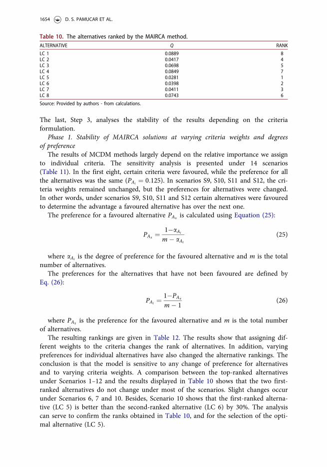
The values of criteria functions (Qi) by alternatives (Table 10) is the sum of the gaps(gij) by alternatives, i.e., the sum of the matrix elements (G) by columns, Equation (23).

Preferably, the alternative should have the lowest possible value of the total gap(alternative no. 5).

4. Sensitivity analysis

The sensitivity analysis of the MAIRCA method is carried out in three steps. Step 1analyses the stability of a solution, while the weights of the criteria and degrees ofpreference for specific alternatives are varied. Step 2 analyses the stability of a solu-tion depending on the change of a scale representing the values of individual criteria.

Table 8. Real ratings matrix Tr .

ALTERNATIVE

CRITERIA




Table 9. Total gap matrix.

ALTERNATIVE

CRITERIA





The last, Step 3, analyses the stability of the results depending on the criteriaformulation.

Phase 1. Stability of MAIRCA solutions at varying criteria weights and degreesof preference

The results of MCDM methods largely depend on the relative importance we assignto individual criteria. The sensitivity analysis is presented under 14 scenarios(Table 11). In the first eight, certain criteria were favoured, while the preference for allthe alternatives was the same (PAi ¼ 0:125). In scenarios S9, S10, S11 and S12, the cri-teria weights remained unchanged, but the preferences for alternatives were changed.In other words, under scenarios S9, S10, S11 and S12 certain alternatives were favouredto determine the advantage a favoured alternative has over the next one.

The preference for a favoured alternative PAa is calculated using Equation (25):

PAa ¼1�aAi

m� aAi

(25)

where aAi is the degree of preference for the favoured alternative and m is the totalnumber of alternatives.

The preferences for the alternatives that have not been favoured are defined byEq. (26):

PAi ¼1�PAa

m� 1(26)

where PAa is the preference for the favoured alternative and m is the total numberof alternatives.

The resulting rankings are given in Table 12. The results show that assigning dif-ferent weights to the criteria changes the rank of alternatives. In addition, varyingpreferences for individual alternatives have also changed the alternative rankings. Theconclusion is that the model is sensitive to any change of preference for alternativesand to varying criteria weights. A comparison between the top-ranked alternativesunder Scenarios 1–12 and the results displayed in Table 10 shows that the two first-ranked alternatives do not change under most of the scenarios. Slight changes occurunder Scenarios 6, 7 and 10. Besides, Scenario 10 shows that the first-ranked alterna-tive (LC 5) is better than the second-ranked alternative (LC 6) by 30%. The analysiscan serve to confirm the ranks obtained in Table 10, and for the selection of the opti-mal alternative (LC 5).

Table 10. The alternatives ranked by the MAIRCA method.ALTERNATIVE Q RANK

LC 1 0.0889 8LC 2 0.0417 4LC 3 0.0698 5LC 4 0.0849 7LC 5 0.0281 1LC 6 0.0398 2LC 7 0.0411 3LC 8 0.0743 6



Table11.Scenarioswith

varyingcriteria

weigh

tsandpreferencesforcertainalternatives.

SCEN

ARIOS

CRITERIONWEIGHTS

CMT

EID

EICSPPEG

SGITU

RCAA

DCE

DBU

LCTS

RRF

EQTA

IT

Scenario

1w1¼w2¼

…w11

0.091

0.091

0.091

0.091

0.091

0.091

0.091

0.091

0.091

0.091

0.091

Scenario

2w1>w2¼

…w11

0.350

0.065

0.065

0.065

0.065

0.065

0.065

0.065

0.065

0.065

0.065

Scenario

3w2>w1¼…

w11

0.068

0.320

0.068

0.068

0.068

0.068

0.068

0.068

0.068

0.068

0.068

Scenario

4w3,w

4>w1¼

…w11

0.067

0.067

0.200

0.200

0.067

0.067

0.067

0.067

0.066

0.066

0.066

Scenario

5w5,w

6>w1¼

…w11

0.056

0.056

0.056

0.056

0.250

0.250

0.056

0.055

0.055

0.055

0.055

Scenario

6w7,w

8>w1¼

…w11

0.067

0.067

0.067

0.067

0.067

0.067

0.200

0.200

0.066

0.066

0.066

Scenario

7w9,w

10>w1¼

…w11

0.050

0.050

0.050

0.050

0.050

0.050

0.050

0.050

0.350

0.200

0.050

Scenario

8w11>w1¼

…w10

0.065

0.065

0.065

0.065

0.065

0.065

0.065

0.065

0.065

0.065

0.350

Advantageof

thealternativeLC

6–29%

(aLC4¼0.29)

0.109

0.105

0.101

0.097

0.094

0.094

0.093

0.088

0.084

0.071

0.063

Advantageof

thealternativeLC

6–30%

(aLC4¼0.30)

0.109

0.105

0.101

0.097

0.094

0.094

0.093

0.088

0.084

0.071

0.063

Advantageof

thealternativeLC

7–3.2%

(aLC4¼0.032)

0.109

0.105

0.101

0.097

0.094

0.094

0.093

0.088

0.084

0.071

0.063

Advantageof

thealternativeLC

2–1.4%

(aLC4¼0.014)

0.109

0.105

0.101

0.097

0.094

0.094

0.093

0.088

0.084

0.071

0.063

Source:P

rovidedby

authors-from

calculations.


On the other hand, the sensitivity of MCDM methods to varying criterion weightsdoes not provide sufficient information to decide how reliable the MCDM methodresults are. The literature (Anojkumar, Ilangkumaran, & Sasirekha, 2014) offers com-parative analyses by the authors trying to detect the characteristics of the selectionproblem that generate the equality of, or differences in, the solutions of individualMCDM methods. However, the same choice suggested by different methods cannotguarantee the rationality and quality of the given solution.

The next section deals with the problem of objective assessment of the solutionsresulting from the COPRAS, MOORA, PROMETHEE, TOPSIS, ELECTRE andMAIRCA methods, using two conditions the sensitivity analysis is based on. One isthe analysis of consistency of results of the above-listed MCDM methods, dependingon a varying unit of measurement in which the values of individual criteria areexpressed. The other condition is the analysis of the consistency of results, dependingon the formulation of criteria, if the same criterion can be expressed in two norma-tively equivalent ways. Illustrative examples show that some of the methods cannotmeet these requirements.

Phase 2. Independence of value scaleThe independence of value scale (IVS) criterion has been applied in the normative the-

ory of decision-making under risk and uncertainty (French, 1988). In this paper the IVScondition is adjusted to the analysis of the consistency of solutions resulting from theassorted MCDM methods (COPRAS, MOORA, PROMETHEE, TOPSIS and MAIRCA).

The IVS of the results of an MCDM method means that the results we obtainedfrom an MCDM method do not depend on the unit of measurement in which wehave expressed the value of any criterion, on condition that the different units ofmeasurement of the given criteria are interconnected by a linear transformation or apositive affine transformation. For the purposes of this analysis, the initial scale(Table 5) has been modified, generating another scale (Scale 2), linked with Scale 1

Table 12. Alternative rankings under different scenarios.

ALTERNATIVE

SCENARIOS/RANK

S1 S2 S3 S4 S5 S6 S7 S8 S9 S10 S11 S12

LC 1 8 6 8 8 6 7 7 7 8 8 8 8LC 2 4 4 2 4 4 1 2 4 4 4 4 4LC 3 5 5 6 6 5 5 4 8 5 5 5 5LC 4 7 8 7 5 8 8 8 6 7 7 7 7LC 5 1 1 1 1 1 2 3 1 1 2 1 1LC 6 3 3 3 2 2 3 5 3 2 1 3 2LC 7 2 2 4 3 3 4 1 2 3 3 2 3LC 8 6 7 5 7 7 6 6 5 6 6 6 6


Table 13. Scales S1 and S2.NO. LINGUISTIC TERMS S1 S2

1. Very good (VG) (4.5,5,5) (8,9,9)2. Good (G) (3.5,4,4.5) (6,7,8)3. Fair (F) (2.5,3,3.5) (4,5,6)4. Poor (P) (1.5,2,2.5) (2,3,4)5. Very poor (VP) (1,1,1) (1,1,1)

Source: Provided by authors.


Table14.IVS–rankings

ofalternatives.

ALTERN

ATIVE

COPRAS

TOPSIS

MOORA

PROMETHEE

MAIRC

A

S1S2

S1S2

S1S2

S1S2

S1S2

LC1

81.26

879.89

70.3871

70.4141

70.1824

80.1819

7�0

.4198

8�0

.4198

80.0889

80.0889

8LC

297.74

396.70

30.6328

20.6230

30.2450

20.2465

30.1920

40.1920

40.0417

40.0417

4LC

385.98

584.63

50.4339

60.4550

50.2005

50.2003

5�0

.2164

5�0

.2164

50.0698

50.0698

5LC

481.57

779.46

80.3796

80.3823

80.1836

70.1805

8�0

.3529

7�0

.3529

70.0849

70.0849

7LC

5100.0

1100.0

10.6039

30.6252

20.2528

10.2575

10.5097

10.5097

10.0281

10.0281

1LC

697.96

297.34

20.6329

10.6340

10.2445

30.2467

20.2844

20.2844

20.0398

20.0398

2LC

795.19

494.15

40.5567

40.5607

40.2359

40.2375

40.2370

30.2370

30.0411

30.0411

3LC

885.76

683.88

60.4350

50.4247

60.1973

60.1945

6�0

.2339

6�0

.2339

60.0743

60.0743

6

Source:P

rovidedby

authors-from

calculations.


with a positive affine transformation (y ¼ 2x�1). Scale 1 (S1) and Scale 2 (S2) areshown in Table 13.

Scale S2 is used to describe the qualitative criteria CMT, EI, CSPPEGS, DBULC,TS and EQTAIT. A comparison was then made between the results of the MCDMmethods (rankings of the alternatives) that were obtained using S1 and S2. The crite-ria weights were not changed. The sensitivity (consistency) of the alternative rankingsto a varying value scale is shown in Table 14. The consistency of rankings by theELECTRE method is displayed in Figure 2.

The analysis of the results presented in Table 14 and Figure 2 shows that themethods COPRAS, TOPSIS, MOORA and ELECTRE do not give consistent solutions.These methods demonstrate inconsistency of the rankings, i.e., dependence of thefinal alternative rankings on a change to the value scale. The methods PROMETHEEand MAIRCA provide for consistent solutions. The method ELECTRE demonstratesa change in domination at four alternatives (LC 5, LC 6, LC 7 and LC 8). In Figure2b the grey colour marks the alternatives that recorded change in domination underthe ELECTRE method.

The results indicate that the methods COPRAS, TOPSIS, MOORA and ELECTREdo not satisfy the IVS condition. On the other hand, the results of the PROMETHEEand MAIRCA methods do not change if the value scale changes.

Phase 3. Independence of criteria formulationThe independence of criteria formulation (ICF) condition is modelled after the

descriptive invariability condition, which in the behavioural theory of decision-mak-ing is defined as the rationality of choice by an individual decision-maker(Kahneman & Tversky, 1981). If there is more than one way to present the alterna-tives, and if these ways are normatively equivalent, a rational individual’s preferencesto these alternatives should not depend on the selected formulation, i.e., they shouldbe independent of the so-called frame.

If this level of rationality is required from the individual decision-maker, it is onlylogical that the MCDM methods we use to support rational decision-making shouldsatisfy the same condition. As some criteria can be presented in both frames (benefit-

Figure 2. IVS – ELECTRE method. Source: Provided by authors - from calculations.


and cost-related), the benefit formulation (benefit-type criteria) will be treated as the‘positive frame’ and the cost formulation (cost-type criteria) as the ‘negative frame’.In addition, the results of an MCDM method should be resistant to the changes inthe formulation of these criteria.

This research has identified three criteria that can be presented in two normativelyequivalent ways, i.e., as benefit-type and cost-type criteria. These are EID, RC and RRF.

The EID is expressed in the percentages describing the estimated levels of infra-structure development. Accordingly, the EID can be expressed as a benefit-type criter-ion (a degree of infrastructure development expressed as a percentage, Xþ) and as acost-type criterion (a degree of infrastructure underdevelopment expressed as a per-centage, X�). As the percentages of infrastructure development and infrastructureunderdevelopment add to 100% (Xþ þ X� ¼ 100%), the two formulations are norma-tively equivalent.

The RC criterion can be expressed as a benefit-type criterion (the maximum num-ber of ITUs that can be reloaded within an hour, ITU/h), and as a cost-type criterion(the time needed for ITU reload). The numerical values of the two formulations areconnected with the function X� ¼ 60=Xþ, where Xþ is the maximum number ofITUs that can be reloaded within an hour (ITU/h), while X�is the time needed toreload one ITU (min/ITU).

The RRF criterion. The maximum required length of a railway reload front is 720m. Based on this information, the RRF can be expressed as a benefit-type criterion(the existing length of the railway reload front, Xþ), and as a cost-type criterion (themissing length of the railway reload front, X�). As the existing length of the railwayreload front and the missing length of the railway reload front add up to720 (Xþ þ X� ¼ 720).

As shown, the EID and RRF criteria can be observed as special cases of the affinetransformation. As these are the special cases of the affine transformation explainedin the previous section (Phase 2. independence of value scale) the change of EID andRRF criteria formulation won’t be considered independently. Scenario 1 will focus onthe independent effect of different formulations of the RC criteria on the consistencyof the results provided by MCDM methods. Scenarios 2, 4 and 6 will address theimpact of changes of the RC criteria formulations on the consistency of the MCDMmethod results with the simultaneous change of EID or RRF criteria formulation.

Seven scenarios have been considered in this analysis. The description and resultsof the scenarios are presented in the following part of the paper.

Scenario 1. MCDM results were compared when the RC criterion was presented asa benefit-type criterion (Scale 1, S1), and as a cost-type criterion (Scale 1, S1). Thevalues of the other criteria remained unchanged (Table 6). The results of the consist-ency of the MCDM methods based on the condition from Scenario 1 are presentedin Table 15.

Scenario 2. The MCDM results were compared when the EID and RC criteria werepresented as cost-type criteria (Scale 2, S2). The values of the other criteria remainedunchanged (Table 6). The results were compared to those obtained when the EIDand RC criteria were presented as benefit-type criteria (Scale 1, S1). The consistencyresults under the Scenario 2 are presented in Table 16.


Table15.ICFScenario

1–rankings

ofalternatives.

ALTERN

ATIVE

COPRAS

TOPSIS

MOORA

PROMETHEE

MAIRC

A

S1S2

S1S2

S1S2

S1S2

S1S2

LC1

81.26

881.27

80.3871

70.3920

70.1824

80.1171

8�0

,4198

8�0

,4198

80.0889

80.0821

8LC

297.74

397.73

30.6328

20.6366

10.2450

20.1796

20,1920

40,1920

40.0417

40.0379

4LC

385.98

585.91

50.4339

60.4362

50.2005

50.1347

5�0

,2164

5�0

,2164

50.0698

50.0645

5LC

481.57

781.50

70.3796

80.3855

80.1836

70.1182

7�0

,3529

7�0

,3529

70.0849

70.0786

7LC

5100.0

1100.0

10.6039

30.6053

30.2528

10.1863

10,5097

10,5097

10.0281

10.0263

1LC

697.96

297.96

20.6329

10.6350

20.2445

30.1784

30,2844

20,2844

20.0398

20.0370

2LC

795.19

495.14

40.5567

40.5616

40.2359

40.1705

40,2370

30,2370

30.0411

30.0376

3LC

885.76

685.74

60.4350

50.4331

60.1973

60.1301

6�0

,2339

6�0

,2339

60.0743

60.0696

6

Source:P

rovidedby

authors-from

calculations.

Table16.ICFScenario

2–rankings

ofalternatives.

ALTERN

ATIVE

COPRAS

TOPSIS

MOORA

PROMETHEE

MAIRC

A

S1S2

S1S2

S1S2

S1S2

S1S2

LC1

81.26

876.74

80.3871

70.3922

70.1824

80.0333

8�0

,4198

8�0

,4198

80.0889

80.0877

8LC

297.74

397.60

20.6328

20.6486

10.2450

20.1154

20,1920

40,1920

40.0417

40.0405

4LC

385.98

582.71

60.4339

60.4491

60.2005

50.0575

6�0

,2164

5�0

,2164

50.0698

50.0689

5LC

481.57

777.05

70.3796

80.3750

80.1836

70.0355

7�0

,3529

7�0

,3529

70.0849

70.0838

7LC

5100.0

1100.0

10.6039

30.6380

30.2528

10.1215

10,5097

10,5097

10.0281

10.0281

1LC

697.96

296.87

30.6329

10.6423

20.2445

30.1099

30,2844

20,2844

20.0398

20.0395

2LC

795.19

493.29

40.5567

40.5724

40.2359

40.1001

40,2370

30,2370

30.0411

30.0401

3LC

885.76

683.20

50.4350

50.4572

50.1973

60.0578

5�0

,2339

6�0

,2339

60.0743

60.0743

6

Source:P

rovidedby

authors-from

calculations.

Table17.ICFScenario

3–rankings

ofalternatives.

ALTERN

ATIVE

COPRAS

TOPSIS

MOORA

PROMETHEE

MAIRC

A

S1S2

S1S2

S1S2

S1S2

S1S2

LC1

81.26

875.68

70.3871

70.3995

60.1824

80.0615

7�0

,4198

8�0

,4198

80.0889

80.0877

8LC

297.74

394.22

30.6328

20.6302

30.2450

20.1350

30,1920

40,1920

40.0417

40.0405

4LC

385.98

584.08

50.4339

60.5042

50.2005

50.0943

5�0

,2164

5�0

,2164

50.0698

50.0689

5LC

481.57

774.74

80.3796

80.3613

80.1836

70.0568

8�0

,3529

7�0

,3529

70.0849

70.0838

7LC

5100.0

1100.0

10.6039

30.6508

10.2528

10.1503

10,5097

10,5097

10.0281

10.0281

1LC

697.96

295.57

20.6329

10.6477

20.2445

30.1362

20,2844

20,2844

20.0398

20.0395

2LC

795.19

493.15

40.5567

40.6009

40.2359

40.1308

40,2370

30,2370

30.0411

30.0401

3LC

885.76

679.93

60.4350

50.3942

70.1973

60.0705

6�0

,2339

6�0

,2339

60.0743

60.0743

6

Source:Providedby

authors-from

calculations.


Scenario 3. The MCDM results were compared when the RC and RRF criteriawere presented as cost-type criteria (Scale 2, S2). The values of the other criteria, justlike under the previous scenarios, remained unchanged (Table 6). The results werecompared to those obtained when the RC and RRF criteria were presented as benefit-type criteria (Scale 1, S1). The consistency results under the Scenario 3 terms are pre-sented in Table 17.

The analyses presented in Tables 15–17 show that some methods do not retainconsistency of results if the criteria are formulated in two normatively equivalentways. The shaded parts of Tables 15–17 mark the inconsistent rankings.

Under Scenario 1 (Table 15), only the TOPSIS method shows inconsistency ofrankings, while the other methods maintain consistency. In this scenario, a change inthe sequence of top-ranked alternatives is recorded in the TOPSIS method. In add-ition to the top-ranked alternatives, the rankings of alternatives LC 3 and LC 8 alsochanged when the TOPSIS method is used. Under Scenario 1, aside from the TOPSISmethod, all the others showed consistency of rankings.

Under Scenario 2 (Table 16), inconsistency of rankings occurred when the meth-ods COPRAS, TOPSIS, MOORA and ELECTRE were used. The COPRAS method isthe most inconsistent (displaying inconsistency in four rankings), whereas theMOORA and TOPSIS methods had two inconsistent rankings each. The other meth-ods (PROMETHEE and MAIRCA) proved to be stable and maintained stability underthis scenario.

Unlike the first three scenarios, where the ELECTRE method demonstrated stabil-ity, the same method showed changes in the domination of alternatives under

Table 18. Analysis of sensitivity of methods to the change of value scale and criteria formulation.SCENARIO COPRAS TOPSIS MOORA PROMETHEE MAIRCA ELECTRE

IVS x x x � � xICF Scenario 1 � x � � � �ICF Scenario 2 x x x � � xICF Scenario 3 x x x � � �

Sources: Provided by authors - from calculations.

Figure 3. ICF Scenario 2 – ELECTRE method. Sources: Provided by authors - from calculations.


Scenario 2 (Figures 3a and 3b). The changes in the domination of alternatives thatoccurred under Scenario 2 are the same as in Phase 2 (Figures 2a and 2b).

Under Scenario 3 (Table 17), the TOPSIS method is the most inconsistent one(showed inconsistency of six rankings). Under this scenario the rankings of the topthree alternatives changed when TOPSIS was used. This shows that the TOPSISmethod considerably violates the consistency of rankings as the formulation of crite-ria changes.

It is noteworthy, however, that no change was recorded to the first-ranked alterna-tive LC 5 under this scenario, when the COPRAS and MOORA methods were used.The methods PROMETHEE, ELECTRE and MAIRCA demonstrated stability of thesolutions under Scenario 3.

The conclusion is that the methods COPRAS, TOPSIS, MOORA and ELECTREare sensitive to a change to the criteria formulation (do not satisfy the ICF condi-tion), whereas the PROMETHEE and MAIRCA do satisfy the ICF condition. Basedon the presented analyses, the results were systematised as follows (Table 18).

In Table 18, symbol ‘x’ indicates that the method does not satisfy the defined con-ditions of sensibility and symbol ‘�’ that it does.

Based on the results of the sensitivity analysis (Table 18), the solutions resultingfrom the MAIRCA and PROMETHEE methods are proven to be stable. Both meth-ods recommend the first-ranked alternative LC 5.

The method ELECTRE demonstrates sensitivity to a change to the value scaleunder the ICF Scenario 2. However, the inconsistency of solutions that occurs whenthe ELECTRE method is used (Figures 2b and 3b) affects only the increasing domin-ance of first-ranked alternatives over the others. Such changes do not affect thechange of an initial solution (Figures 2a and 3a), but confirm additionally the domin-ation of first-ranked alternatives (LC 5 and LC 6) over the others.

The COPRAS and MOORA methods demonstrate sensitivity to a varying valuescale and to the changing formulation of attributes. Inconsistency was recorded inseven of eight cases (Table 18). The inconsistency, however, didn’t change the first-ranked alternative. In all cases, LC 5 was the first-ranked alternative.

When the TOPSIS method was used, the top-ranked alternatives changed in six ofeight cases. It proves that TOPSIS significantly violates the consistency of rankings.Owing to this problem, the sequence of alternatives suggested by the TOPSIS methodwas not considered while making a final choice of the LC location.

As LC 5 was the first-ranked alternative when, MOORA, MAIRCA, ELECTRE andPROMETHEE were used, we can conclude that LC 5 is the optimal alternative.

5. Conclusion

This paper presents the application of the hybrid DEMATEL–MAIRCA model in adecision-making process aimed to select the location of a multimodal logistics centre(LC) by the Danube River (Transportation Corridor IX). The DEMATEL method wasused to specify the weights of criteria, and a new multi-criteria method, MAIRCA, tovalue the alternatives and select the LC location. The application of the two methodswas presented in consecutive steps and illustrated by examples.


After the MAIRCA method was applied, a sensitivity analysis was performed inthree phases. In Phase 1, the stability of MAIRCA solutions was analysed, dependingon varying criteria weights preferences for individual alternatives. In Phases 2 and 3,a consistency analysis was carried out and the results of several MCDM methods(COPRAS, TOPSIS, MOORA, PROMETHEE and ELECTRE) were compared. Theresults of these MCDM methods were compared to the results obtained when theMAIRCA method was used. Two conditions to provide for the rationality of aMCDM choice were made based on the consistency of final results. One is the con-sistency of MCDM results depending on changing the unit of measurement in whichthe values of individual criteria was expressed. The other is the analysis of consistencyof the results depending on the formulation of criteria, if the same criteria can bepresented in two normatively equivalent ways – as benefit- and cost-type criteria.Based on these results, COPRAS, TOPSIS, MOORA and ELECTRE were found notto satisfy between one and all five conditions, whereas MAIRCA and PROMETHEEshowed consistency in all cases.

According to the results of the sensitivity analysis presented in this paper, it canbe concluded that MAIRCA has a stable and well-structured analytical framework forranking the alternatives. Relaying the presented application of MAIRCA method andsensitivity analysis that was conducted, the following advantages of MAIRCA can besingled out: (1) the method’s mathematical framework remains the same regardless ofthe number of alternatives and criteria; (2) the possibility of MAIRCA application ina case of a large number of alternatives and criteria; (3) the clearly defined alternativerank presented by numerical value, enabling easier comprehension of results; (4)applicability to qualitative and quantitative criteria type; (5) the method takes intoaccount the distance between ideal and anti-ideal solutions; and (6) the method givesstable solutions regardless of changes in the qualitative criteria measurement scaleand changes in quantitative criteria formulation.

Apart from the application in LC location selection, MAIRCA can be used in otherproblems involving multi-criteria decision-making. The principal recommendation forfurther use of this method is a simple mathematical apparatus, consistency of solu-tions and the possibility of combining it with other methods, especially when criteriaweights are to be specified.

Disclosure statement

No potential conflict of interest was reported by the authors.

References

Anojkumar, L., Ilangkumaran, M., & Sasirekha, V. (2014). Comparative analysis of MCDMmethods for pipe material selection in sugar industry. Expert Systems with Applications, 41,2964–2980.

Badi I., & Ballem, M. (2018). Supplier selection using rough BWM-MAIRCA model: A casestudy in pharmaceutical supplying in Libya. Decision Making: Applications in Managementand Engineering, 1(2), 15–32. doi:10.31181/dmame1802016b

Brimberg, J., Drezner, Z., Mladenovi�c, N., & Salhi, S. (2014). A new local search for continu-ous location problems. European Journal of Operational Research, 232(2), 256–265.


https://doi.org/10.31181/dmame1802016b

Camparo, J. (2013). A geometrical approach to the ordinal data of Likert scaling and attitudemeasurements: The density matrix in psychology. Journal of Mathematical Psychology, 57,29–42.

Chen S., & Liu, X. (2006). Factors and a method of selecting a site for a logistical centre.Journal of Weinan Teachers College, 3.

Dalalah, D., Hayajneh, M., & Batieha, F. (2011). A fuzzy multi-criteria decision making modelfor supplier selection. Expert Systems with Applications, 38, 8384–8391.

Erlenkotter, D. (1978). A dual-based procedure for uncapacitated facility location. OperationsResearch, 26(6), 992–1009.

French, S. (1988). Decision theory - an introduction to the mathematics of rationality.Chrichster: Ellis Horwood Ltd.

Han H, Li B, Wang K.F., & Shi Z (2016). Exploiting structural similarity of log files in faultdiagnosis for web service composition. CAAI Transactions on Intelligence Technology, 1(1),61–71.

Jan�a�cek, J., & Buzna, L. (2008). An acceleration of Erlenkotter–K€orkel’s algorithms for theuncapacitated facility location problem. Annals of Operations Research, 164(1), 97–109.

Ji, W., Tang, L., Li, D., Yang, W., & Liao, Q. (2016). Video-based construction vehicles detec-tion and its application in intelligent monitoring system. CAAI Transactions on IntelligenceTechnology, 1(2), 162–172.

Kahneman, D., & Tversky, A. (1981). The framing of decisions and the psychology of choice.Science, 211(4481), 453–458.

Kannan G., Noorul Haq, P., & Sasikumar, P. (2008). An application of the analytical hierarchyprocess and Fuzzy analytical hierarchy process in the selection of collecting centre locationfor the reverse logistics multi-criteria decision-making supply chain model. InternationalJournal of Management and Decision Making, 9(4), 350–365.

Kracka, M., Brauers, W. K. M., & Zavadskas, E. K. (2010). Ranking heating losses in a buildingby applying the MULTIMOORA. Inzinerine Ekonomika-Engineering Economics, 21(4),352–359.

Li, Q. (2013). A novel Likert scale based on fuzzy sets theory. Expert Systems withApplications, 40, 1609–1618.

Liu, Z., Wang, W., & Jin, Q. (2016c). Manifold alignment using discrete surface Ricci flow.CAAI Transactions on Intelligence Technology, 1(3), 285–292.

Milosavljevic, M., Bursa�c, M. & Tri�ckovi�c, G. (2018). The selection of the railroad containerterminal in Serbia based on multi criteria decision making methods. Decision Making:Applications in Management and Engineering, 1(2), 1–14.

Mladenovi�c, N., Brimberg, J., Hansen, P., & Moreno-P�erez, J. A. (2017). The p-median prob-lem: A survey of metaheuristic approaches. European Journal of Operational Research,179(3), 927–939.

Ou, C.-W., & Chou, S.-Y. (2009). International distribution centre selection from a foreignmarket perspective using a weighted fuzzy factor rating system. Expert System withApplications, 36(2), 1773–1782.

Pamu�car, D., & �Cirovi�c, Y. (2015). The selection of transport and handling resources in logis-tics centres using Multi-Attributive Border Approximation area Comparison (MABAC).Expert Systems with Applications, 42, 3016–3028. doi: 10.1016/j.eswa.2014.11.057

Petrovi�c, I., & Kankara�s, M. (2018). DEMATEL-AHP multi-criteria decision making model forthe selection and evaluation of criteria for selecting an aircraft for the protection of airtraffic. Decision Making: Applications in Management and Engineering, 1(2), 91–108. doi:10.31181/dmame1802091p

Qazi, K., Lam, H.K., Xiao, B., Ouyang, G., Yin, X. (2016). Classification of epilepsy using com-putational intelligence techniques. CAAI Transactions on Intelligence Technology, 1(2),137–149.

Rezaeiniya, N., Zolfani, S. H., & Zavadskas, E. K. (2012). Greenhouse locating based on ANP-COPRAS-G methods - an empirical study based on Iran. International Journal of StrategicProperty Management, 16(2), 188–200.


https://doi.org/10.1016/j.eswa.2014.11.057

https://doi.org/10.31181/dmame1802091p

Sirikijpanichkul, A., & Ferreira, L. (2006). Modeling intermodal freight hub location decisions.2006 IEEE International Conference on Systems,Man and Cybernetics, Oct. 8-11, Taipei,Taiwan.

Turskis, Z., Zavadskas, E. K., Antucheviciene, J., Kosareva, N. (2015). A Hybrid Model Basedon Fuzzy AHP and Fuzzy WASPAS for Construction Site Selection. International Journal ofComputers Communications & Control, 10(6), 873–888.

Vasiljevic, M., Fazlollahtabar, H., Stevic, Z., & Veskovic, S. (2018). A rough multicriteriaapproach for evaluation of the supplier criteria in automotive industry. Decision Making:Applications in Management and Engineering, 1(1), 82–96. doi:10.31181/dmame180182v

Wan, L., Huang, Z., & Li, Z. (2007). Research of optimal Dijkstra algorithm in logistic centerlocation based on GIS. Application Research of Computers, 8(24), 289–291.

Wang, X., Li, L., Yuan, Y., Ye, P., & Wang, F. Y. (2016b). ACP-based social computing andparallel intelligence: Societies 5.0 and beyond. CAAI Transactions on Intelligence Technology,1(4), 377–393.

Xu, X., Law, R., Chen, W. & Tang, L. (2016a). Forecasting tourism demand by extracting fuzzyTakagi-Sugeno rules from trained SVMs. CAAI Transactions on Intelligence Technology,1(1), 30–42. http://dx.doi.org/10.1016/j.trit.2016.03.004

Xu, Y., Dong, J., Zhang, B., & Xu, D. (2016b). Background modeling methods in video ana-lysis: A review and comparative evaluation. CAAI Transactions on Intelligence Technology,1(1), 43–60.

Yang, J., & Lee, H. (1997). An AHP decision model for facility location selection. Facilities,15(9/10), 241–254.

Yang, W., Sun, X., Deng, W., Zhang, C., Liao, Q. (2016). Fourier locally linear soft constrainedMACE for facial landmark localization. CAAI Transactions on Intelligence Technology, 1(3),241–248.

Zavadskas, E.K., Turskis, Z., Bago�cius, V. (2015). Multi-criteria selection of a deep-water portin the Eastern Baltic Sea. Applied Soft Computing, 26, 180–192.

Zecevic, S. (2006). Cargo Terminals and Cargo Transport Centers, Faculty of Transportation,Belgrade University.

Zhang, Q., Xie, Q., Wang, G. (2016). A survey on rough set theory and its applications. CAAITransactions on Intelligence Technology, 1(4), 323–333.


https://doi.org/10.31181/dmame180182v

http://dx.doi.org/10.1016/j.trit.2016.03.004

new hybrid multi-criteria decision-making dematel-mairca

Documents