new inference rules for max-sat · 2009-02-08 · new inference rules for max-sat formula φ′ =...
TRANSCRIPT
Journal of Artificial Intelligence Research 30 (2007) 321–359 Submitted 11/06; published 10/07
New Inference Rules for Max-SAT
Chu Min Li [email protected]
LaRIA, Universite de Picardie Jules Verne
33 Rue St. Leu, 80039 Amiens Cedex 01, France
Felip Manya [email protected]
IIIA, Artificial Intelligence Research Institute
CSIC, Spanish National Research Council
Campus UAB, 08193 Bellaterra, Spain
Jordi Planes [email protected]
Computer Science Department, Universitat de Lleida
Jaume II, 69, 25001 Lleida, Spain
Abstract
Exact Max-SAT solvers, compared with SAT solvers, apply little inference at eachnode of the proof tree. Commonly used SAT inference rules like unit propagation producea simplified formula that preserves satisfiability but, unfortunately, solving the Max-SATproblem for the simplified formula is not equivalent to solving it for the original formula.In this paper, we define a number of original inference rules that, besides being appliedefficiently, transform Max-SAT instances into equivalent Max-SAT instances which areeasier to solve. The soundness of the rules, that can be seen as refinements of unit resolutionadapted to Max-SAT, are proved in a novel and simple way via an integer programmingtransformation. With the aim of finding out how powerful the inference rules are in practice,we have developed a new Max-SAT solver, called MaxSatz, which incorporates those rules,and performed an experimental investigation. The results provide empirical evidence thatMaxSatz is very competitive, at least, on random Max-2SAT, random Max-3SAT, Max-Cut, and Graph 3-coloring instances, as well as on the benchmarks from the Max-SATEvaluation 2006.
1. Introduction
In recent years there has been a growing interest in developing fast exact Max-SATsolvers (Alber, Gramm, & Niedermeier, 2001; Alsinet, Manya, & Planes, 2003b, 2005;de Givry, Larrosa, Meseguer, & Schiex, 2003; Li, Manya, & Planes, 2005; Xing & Zhang,2004; Zhang, Shen, & Manya, 2003) due to their potential to solve over-constrained NP-hard problems encoded in the formalism of Boolean CNF formulas. Nowadays, Max-SATsolvers are able to solve a lot of instances that are beyond the reach of the solvers developedjust five years ago. Nevertheless, there is yet a considerable gap between the difficulty of theinstances solved with current SAT solvers and the instances solved with the best performingMax-SAT solvers.
The motivation behind our work is to bridge that gap between complete SAT solversand exact Max-SAT solvers by investigating how the technology previously developed forSAT (Goldberg & Novikov, 2001; Li, 1999; Marques-Silva & Sakallah, 1999; Zhang, 1997;Zhang, Madigan, Moskewicz, & Malik, 2001) can be extended and incorporated into Max-
c©2007 AI Access Foundation. All rights reserved.
Li, Manya & Planes
SAT. More precisely, we focus the attention on branch and bound Max-SAT solvers based onthe Davis-Putnam-Logemann-Loveland (DPLL) procedure (Davis, Logemann, & Loveland,1962; Davis & Putnam, 1960).
One of the main differences between SAT solvers and Max-SAT solvers is that the formermake an intensive use of unit propagation at each node of the proof tree. Unit propagation,which is a highly powerful inference rule, transforms a SAT instance φ into a satisfiabilityequivalent SAT instance φ′ which is easier to solve. Unfortunately, solving the Max-SATproblem for φ is, in general, not equivalent to solving it for φ′; i.e., the number of unsatisfiedclauses in φ and φ′ is not the same for every truth assignment. For example, if we applyunit propagation to the CNF formula φ = {x1, x1 ∨ x2, x1 ∨ ¬x2, x1 ∨ x3, x1 ∨ ¬x3}, weobtain φ′ = {2, 2}, but φ and φ′ are not equivalent because any interpretation satisfying¬x1 unsatisfies one clause of φ and two clauses of φ′. Therefore, if we want to compute anoptimal solution, we cannot apply unit propagation as in SAT solvers.
We proposed in a previous work (Li et al., 2005) to use unit propagation to computelower bounds in branch and bound Max-SAT solvers instead of using unit propagation tosimplify CNF formulas. In our approach, we detect disjoint inconsistent subsets of clausesvia unit propagation. It turns out that the number of disjoint inconsistent subsets detectedis an underestimation of the number of clauses that will become unsatisfied when the currentpartial assignment is extended to a complete assignment. That underestimation plus thenumber of clauses unsatisfied by the current partial assignment provides a good performinglower bound, which captures the lower bounds based on inconsistency counts that most ofthe state-of-the-art Max-SAT solvers implement (Alsinet, Manya, & Planes, 2003a; Alsinetet al., 2003b; Borchers & Furman, 1999; Wallace & Freuder, 1996; Zhang et al., 2003), aswell as other improved lower bounds (Alsinet, Manya, & Planes, 2004; Alsinet et al., 2005;Xing & Zhang, 2004, 2005).
On the one hand, the number of disjoint inconsistent subsets detected is just a conser-vative underestimation for the lower bound, since every inconsistent subset φ increases thelower bound by one independently of the number of clauses of φ unsatisfied by an optimalassignment. However, an optimal assignment can violate more than one clause of an incon-sistent subset. Therefore, we should be able to improve the lower bound based on countingthe number of disjoint inconsistent subsets of clauses.
On the other hand, despite the fact that good quality lower bounds prune large parts ofthe search space and accelerate dramatically the search for an optimal solution, wheneverthe lower bound does not reach the best solution found so far (upper bound), the solvercontinues exploring the search space below the current node. During that search, solversoften redetect the same inconsistencies when computing the lower bound at different nodes.Basically, the problem with lower bound computation methods is that they do not simplifythe CNF formula in such a way that the unsatisfied clauses become explicit. Lower boundsare just a pruning technique.
To overcome the above two problems, we define a set of sound inference rules thattransform a Max-SAT instance φ into a Max-SAT instance φ′ which is easier to solve. InMax-SAT, an inference rule is sound whenever φ and φ’ are equivalent.
Let us see an example of inference rule: Given a Max-SAT instance φ that containsthree clauses of the form l1, l2, l1 ∨ l2, where l1, l2 are literals, we replace φ with the CNF
322
New Inference Rules for Max-SAT
formula
φ′ = (φ− {l1, l2, l1 ∨ l2}) ∪ {2, l1 ∨ l2}.
Note that the rule detects a contradiction from l1, l2, l1 ∨ l2 and, therefore, replaces theseclauses with an empty clause. In addition, the rule adds the clause l1 ∨ l2 to ensure theequivalence between φ and φ′. For any assignment containing either l1 = 0, l2 = 1, orl1 = 1, l2 = 0, or l1 = 1, l2 = 1, the number of unsatisfied clauses in {l1, l2, l1 ∨ l2} is 1,but for any assignment containing l1 = 0, l2 = 0, the number of unsatisfied clauses is 2.Note that even when any assignment containing l1 = 0, l2 = 0 is not the best assignmentfor the subset {l1, l2, l1 ∨ l2}, it can be the best for the whole formula. By adding l1 ∨ l2,the rule ensures that the number of unsatisfied clauses in φ and φ′ is also the same whenl1 = 0, l2 = 0.
That inference rule adds the new clause l1 ∨ l2, which may contribute to another con-tradiction detectable via unit propagation. In this case, the rule allows to increase thelower bound by 2 instead of 1. Moreover, the rule makes explicit a contradiction amongl1, l2, l1 ∨ l2, so that the contradiction does not need to be redetected below the currentnode.
Some of the inference rules defined in the paper are already known in the litera-ture (Bansal & Raman, 1999; Niedermeier & Rossmanith, 2000), others are original forMax-SAT. The new rules were inspired by different unit resolution refinements applied inSAT, and were selected because they could be applied in a natural and efficient way. In asense, we can summarize our work telling that we have defined the Max-SAT counterpartof SAT unit propagation.
With the aim of finding out how powerful the inference rules are in practice, we havedesigned and implemented a new Max-SAT solver, called MaxSatz, which incorporates thoserules, as well as the lower bound defined in a previous work (Li et al., 2005), and performedan experimental investigation. The results provide empirical evidence that MaxSatz is verycompetitive, at least, on random Max-2SAT, random Max-3SAT, Max-Cut, and Graph3-coloring instances, as well as on the benchmarks from the Max-SAT Evaluation 20061.
The structure of the paper is as follows. In Section 2, we give some preliminary defini-tions. In Section 3, we describe a basic branch and bound Max-SAT solver. In Section 4, wedefine the inference rules and prove their soundness in a novel and simple way via an integerprogramming transformation. We also give examples to illustrate that the inference rulesmay produce better quality lower bounds. In Section 5, we present the implementation ofthe inference rules in MaxSatz. In Section 6, we describe the main features of MaxSatz. InSection 7, we report on the experimental investigation. In Section 8, we present the relatedwork. In Section 9, we present the conclusions and future work.
2. Preliminaries
In propositional logic a variable xi may take values 0 (for false) or 1 (for true). A literal liis a variable xi or its negation xi. A clause is a disjunction of literals, and a CNF formulaφ is a conjunction of clauses. The length of a clause is the number of its literals. The sizeof φ, denoted by |φ|, is the sum of the length of all its clauses.
1. http://www.iiia.csic.es/˜maxsat06
323
Li, Manya & Planes
An assignment of truth values to the propositional variables satisfies a literal xi if xi
takes the value 1 and satisfies a literal xi if xi takes the value 0, satisfies a clause if itsatisfies at least one literal of the clause, and satisfies a CNF formula if it satisfies all theclauses of the formula. An empty clause, denoted by 2, contains no literals and cannot besatisfied. An assignment for a CNF formula φ is complete if all the variables occurring inφ have been assigned; otherwise, it is partial.
The Max-SAT problem for a CNF formula φ is the problem of finding an assignmentof values to propositional variables that minimizes the number of unsatisfied clauses (orequivalently, that maximizes the number of satisfied clauses). Max-SAT is called Max-kSAT when all the clauses have k literals per clause. In the following, we represent a CNFformula as a multiset of clauses, since duplicated clauses are allowed in a Max-SAT instance.
CNF formulas φ1 and φ2 are equivalent if φ1 and φ2 have the same number of unsatisfiedclauses for every complete assignment of φ1 and φ2.
3. A Basic Max-SAT Solver
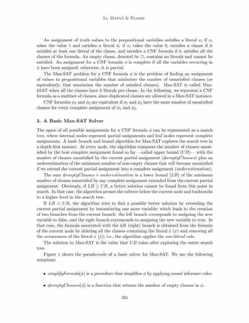
The space of all possible assignments for a CNF formula φ can be represented as a searchtree, where internal nodes represent partial assignments and leaf nodes represent completeassignments. A basic branch and bound algorithm for Max-SAT explores the search tree ina depth-first manner. At every node, the algorithm compares the number of clauses unsat-isfied by the best complete assignment found so far —called upper bound (UB)— with thenumber of clauses unsatisfied by the current partial assignment (#emptyClauses) plus anunderestimation of the minimum number of non-empty clauses that will become unsatisfiedif we extend the current partial assignment into a complete assignment (underestimation).
The sum #emptyClauses + underestimation is a lower bound (LB) of the minimumnumber of clauses unsatisfied by any complete assignment extended from the current partialassignment. Obviously, if LB ≥ UB, a better solution cannot be found from this point insearch. In that case, the algorithm prunes the subtree below the current node and backtracksto a higher level in the search tree.
If LB < UB, the algorithm tries to find a possible better solution by extending thecurrent partial assignment by instantiating one more variable; which leads to the creationof two branches from the current branch: the left branch corresponds to assigning the newvariable to false, and the right branch corresponds to assigning the new variable to true. Inthat case, the formula associated with the left (right) branch is obtained from the formulaof the current node by deleting all the clauses containing the literal x (x) and removing allthe occurrences of the literal x (x); i.e., the algorithm applies the one-literal rule.
The solution to Max-SAT is the value that UB takes after exploring the entire searchtree.
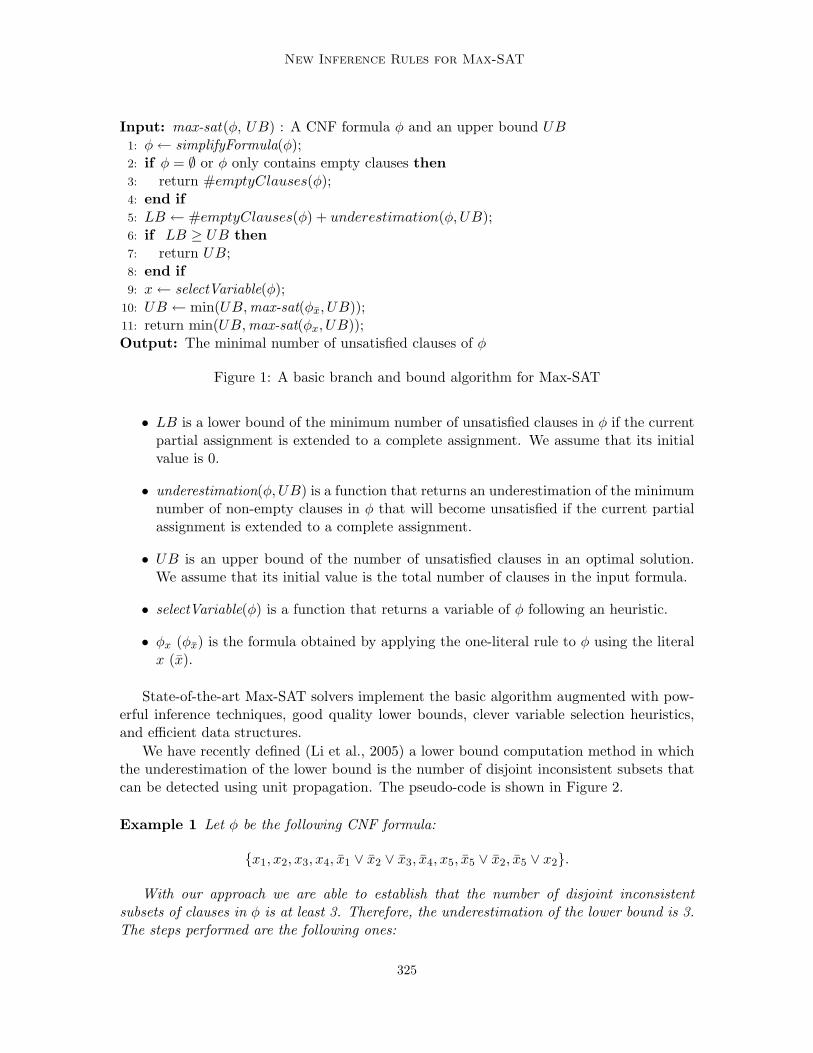
Figure 1 shows the pseudo-code of a basic solver for Max-SAT. We use the followingnotations:
• simplifyFormula(φ) is a procedure that simplifies φ by applying sound inference rules.
• #emptyClauses(φ) is a function that returns the number of empty clauses in φ.
324
New Inference Rules for Max-SAT
Input: max-sat(φ, UB) : A CNF formula φ and an upper bound UB
1: φ← simplifyFormula(φ);2: if φ = ∅ or φ only contains empty clauses then3: return #emptyClauses(φ);4: end if5: LB ← #emptyClauses(φ) + underestimation(φ, UB);6: if LB ≥ UB then7: return UB;8: end if9: x← selectVariable(φ);
10: UB ← min(UB,max-sat(φx, UB));11: return min(UB,max-sat(φx, UB));Output: The minimal number of unsatisfied clauses of φ
Figure 1: A basic branch and bound algorithm for Max-SAT
• LB is a lower bound of the minimum number of unsatisfied clauses in φ if the currentpartial assignment is extended to a complete assignment. We assume that its initialvalue is 0.
• underestimation(φ, UB) is a function that returns an underestimation of the minimumnumber of non-empty clauses in φ that will become unsatisfied if the current partialassignment is extended to a complete assignment.
• UB is an upper bound of the number of unsatisfied clauses in an optimal solution.We assume that its initial value is the total number of clauses in the input formula.
• selectVariable(φ) is a function that returns a variable of φ following an heuristic.
• φx (φx) is the formula obtained by applying the one-literal rule to φ using the literalx (x).
State-of-the-art Max-SAT solvers implement the basic algorithm augmented with pow-erful inference techniques, good quality lower bounds, clever variable selection heuristics,and efficient data structures.
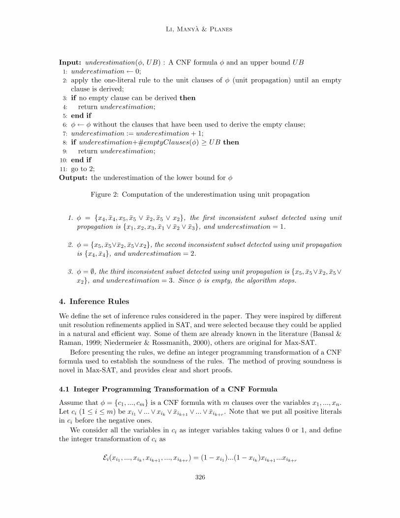
We have recently defined (Li et al., 2005) a lower bound computation method in whichthe underestimation of the lower bound is the number of disjoint inconsistent subsets thatcan be detected using unit propagation. The pseudo-code is shown in Figure 2.
Example 1 Let φ be the following CNF formula:
{x1, x2, x3, x4, x1 ∨ x2 ∨ x3, x4, x5, x5 ∨ x2, x5 ∨ x2}.
With our approach we are able to establish that the number of disjoint inconsistentsubsets of clauses in φ is at least 3. Therefore, the underestimation of the lower bound is 3.The steps performed are the following ones:
325
Li, Manya & Planes
Input: underestimation(φ, UB) : A CNF formula φ and an upper bound UB
1: underestimation← 0;2: apply the one-literal rule to the unit clauses of φ (unit propagation) until an empty
clause is derived;3: if no empty clause can be derived then4: return underestimation;5: end if6: φ← φ without the clauses that have been used to derive the empty clause;7: underestimation := underestimation + 1;8: if underestimation+#emptyClauses(φ) ≥ UB then9: return underestimation;
10: end if11: go to 2;Output: the underestimation of the lower bound for φ
Figure 2: Computation of the underestimation using unit propagation
1. φ = {x4, x4, x5, x5 ∨ x2, x5 ∨ x2}, the first inconsistent subset detected using unitpropagation is {x1, x2, x3, x1 ∨ x2 ∨ x3}, and underestimation = 1.
2. φ = {x5, x5∨x2, x5∨x2}, the second inconsistent subset detected using unit propagationis {x4, x4}, and underestimation = 2.
3. φ = ∅, the third inconsistent subset detected using unit propagation is {x5, x5∨ x2, x5∨x2}, and underestimation = 3. Since φ is empty, the algorithm stops.
4. Inference Rules
We define the set of inference rules considered in the paper. They were inspired by differentunit resolution refinements applied in SAT, and were selected because they could be appliedin a natural and efficient way. Some of them are already known in the literature (Bansal &Raman, 1999; Niedermeier & Rossmanith, 2000), others are original for Max-SAT.
Before presenting the rules, we define an integer programming transformation of a CNFformula used to establish the soundness of the rules. The method of proving soundness isnovel in Max-SAT, and provides clear and short proofs.
4.1 Integer Programming Transformation of a CNF Formula
Assume that φ = {c1, ..., cm} is a CNF formula with m clauses over the variables x1, ..., xn.Let ci (1 ≤ i ≤ m) be xi1 ∨ ...∨xik ∨ xik+1
∨ ...∨ xik+r. Note that we put all positive literals
in ci before the negative ones.
We consider all the variables in ci as integer variables taking values 0 or 1, and definethe integer transformation of ci as
Ei(xi1 , ..., xik , xik+1, ..., xik+r
) = (1− xi1)...(1− xik)xik+1...xik+r
326
New Inference Rules for Max-SAT
Obviously, Ei has value 0 iff at least one of the variables xij ’s (1 ≤ j ≤ k) is instantiatedto 1 or at least one of the variables xis ’s (k + 1 ≤ s ≤ k + r) is instantiated to 0. In otherwords, Ei=0 iff ci is satisfied. Otherwise Ei=1.
A literal l corresponds to an integer denoted by l itself for our convenience. The intentionof the correspondence is that the literal l is satisfied if the integer l is 1 and is unsatisfied ifthe integer l is 0. So if l is a positive literal x, the corresponding integer l is x, l is 1-x=1-l,and if l is a negative literal x, l is 1-x and l is x=1-(1-x)=1-l. Consequently, l=1-l in anycase.
We now generically write ci as l1∨ l2∨ ...∨ lk+r. Its integer programming transformationis
Ei = (1− l1)(1− l2)...(1− lk+r).
The integer programming transformation of a CNF formula φ = {c1, ..., cm} over thevariables x1, ..., xn is defined as
E(x1, ..., xn) =m
∑
i=1
Ei (1)
That integer programming transformation was used (Huang & Jin, 1997; Li & Huang,2005) to design a local search procedure, and is called pseudo-Boolean formulation by Borosand Hammer (2002). Here, we extend it to empty clauses: if ci is empty, then Ei=1.
Given an assignment A over the variables x1, ..., xn, the value of E is the number ofunsatisfied clauses in φ. If A satisfies all clauses in φ, then E = 0. Obviously, the minimumnumber of unsatisfied clauses of φ is the minimum value of E .
Let φ1 and φ2 be two CNF formulas, and let E1 and E2 be their integer programmingtransformations. It is clear that φ1 and φ2 are equivalent if, and only if, E1=E2 for everycomplete assignment for φ1 and φ2.
4.2 Inference Rules
We next define the inference rules and prove their soundness using the previous integerprogramming transformation. In the rest of the section, φ1, φ2 and φ′ denote CNF formulas,and E1, E2, and E ′ their integer programming transformations. To prove that φ1 and φ2 areequivalent, we prove that E1 = E2.
Rule 1 (Bansal & Raman, 1999) If φ1={l1 ∨ l2 ∨ ... ∨ lk, l1 ∨ l2 ∨ ... ∨ lk} ∪ φ′, thenφ2={l2 ∨ ... ∨ lk} ∪ φ′ is equivalent to φ1.
Proof 1
E1 = (1− l1)(1− l2)...(1− lk) + l1(1− l2)...(1− lk) + E ′
= (1− l2)...(1− lk) + E ′
= E2 �
General case resolution does not work in Max-SAT (Bansal & Raman, 1999). Rule 1establishes that resolution works when two clauses give a strictly shorter resolvent.
327
Li, Manya & Planes
Rule 1 is known in the literature as replacement of almost common clauses. We payspecial attention to the case k=2, where the resolvent is a unit clause, and to the case k=1,where the resolvent is the empty clause. We describe this latter case in the following rule:
Rule 2 (Niedermeier & Rossmanith, 2000) If φ1={l, l}∪φ′, then φ2={2}∪φ′ is equivalentto φ1.
Proof 2 E1=1-l+ l+E ′=1+ E ′=E2 �
Rule 2, which is known as complementary unit clause rule, can be used to replace twocomplementary unit clauses with an empty clause. The new empty clause contributes tothe lower bounds of the search space below the current node by incrementing the numberof unsatisfied clauses, but not by incrementing the underestimation, which means that thiscontradiction does not have to be redetected again. In practice, that simple rule gives riseto considerable gains.
The following rule is a more complicated case:
Rule 3 If φ1={l1, l1 ∨ l2, l2} ∪ φ′, then φ2={2, l1 ∨ l2} ∪ φ′ is equivalent to φ1.
Proof 3
E1 = 1− l1 + l1l2 + 1− l2 + E ′
= 1 + 1− l1 + l2(l1 − 1) + E ′
= 1 + 1− l1 − l2(1− l1) + E ′
= 1 + (1− l1)(1− l2) + E ′
= E2 �
Rule 3 replaces three clauses with an empty clause, and adds a new binary clause tokeep the equivalence between φ1 and φ2.
Pattern φ1 was considered to compute underestimations by Alsinet et al. (2004) and Shenand Zhang (2004); and is also captured by our method of computing underestimations basedon unit propagation (Li et al., 2005). Larrosa and Heras mentioned (2005) that existentialdirectional arc consistency (de Givry, Zytnicki, Heras, & Larrosa, 2005) can capture thisrule. Note that underestimation computation methods by Alsinet et al. and Shen andZhang do not add any additional clause as in our approach, they just detect contradictions.
Let us define a rule that generalizes Rule 2 and Rule 3. Before presenting the rule, wedefine a lemma needed to prove its soundness.
Lemma 1 If φ1={l1, l1 ∨ l2} ∪ φ′ and φ2={l2, l2 ∨ l1} ∪ φ′, then φ1 and φ2 are equivalent.
Proof 4
E1 = 1− l1 + l1(1− l2) + E ′
= 1− l1 + l1 − l1l2 + E ′
= 1− l2 + l2 − l1l2 + E ′
= 1− l2 + (1− l1)l2 + E ′
= E2 �
328
New Inference Rules for Max-SAT
Rule 4 If φ1={l1, l1∨l2, l2∨l3, ..., lk∨lk+1, lk+1}∪φ′, then φ2={2, l1∨ l2, l2∨ l3, ..., lk∨lk+1} ∪ φ′ is equivalent to φ1.
Proof 5 We prove the soundness of the rule by induction on k. When k=1, φ1 = {l1, l1 ∨l2, l2}∪φ′. By applying Rule 3, we get {2, l1∨ l2}∪φ′, which is φ2 when k = 1. Therefore,φ1 and φ2 are equivalent.
Assume that Rule 4 is sound for k = n. Let us prove that it is sound for k = n + 1. Inthat case:
φ1 = {l1, l1 ∨ l2, l2 ∨ l3, ..., ln ∨ ln+1, ln+1 ∨ ln+2, ln+2} ∪ φ′.
By applying Lemma 1 to the last two clauses of φ1 (before φ′), we get
{l1, l1 ∨ l2, l2 ∨ l3, ..., ln ∨ ln+1, ln+1, ln+1 ∨ ln+2} ∪ φ′.
By applying the induction hypothesis to the first n+1 clauses of the previous CNF formula,we get
{2, l1 ∨ l2, l2 ∨ l3, ..., ln ∨ ln+1, ln+1 ∨ ln+2} ∪ φ′,
which is φ2 when k = n + 1. Therefore, φ1 and φ2 are equivalent and the rule is sound.�
Rule 4 is an original inference rule. It captures linear unit resolution refutations inwhich clauses and resolvents are used exactly once. The rule simply adds an empty clause,eliminates two unit clauses and the binary clauses used in the refutation, and adds newbinary clauses that are obtained by negating the literals of the eliminated binary clauses.So, all the operations involved can be performed efficiently.
Rule 3 and Rule 4 make explicit a contradiction, which does not need to be redetected inthe current subtree. So, the lower bound computation becomes more incremental. Moreover,the binary clauses added by Rule 3 and Rule 4 may contribute to compute better qualitylower bounds either by acting as premises of an inference rule or by being part of aninconsistent subset of clauses, as is illustrated in the following example.
Example 2 Let φ={x1, x1∨ x2, x3, x3∨x2, x4, x1∨ x4, x3∨ x4}. Depending on the orderingin which unit clauses are propagated, unit propagation detects one of the following threeinconsistent subsets of clauses: {x1, x1 ∨ x2, x3, x3 ∨ x2}, {x1, x4, x1 ∨ x4}, or {x3, x4, x3 ∨x4}. Once an inconsistent subset is detected and removed, the remaining set of clauses issatisfiable. Without applying Rule 3 and Rule 4, the lower bound computed is 1, because theunderestimation computed using unit propagation is 1.
Note that Rule 4 can be applied to the first inconsistent subset {x1, x1 ∨ x2, x3, x3 ∨ x2}.If Rule 4 is applied, a contradiction is made explicit and the clauses x1 ∨x2 and x3 ∨ x2 areadded. So, φ becomes {2, x1 ∨ x2, x3 ∨ x2, x4, x1 ∨ x4, x3 ∨ x4}. It turns out that φ − {2}is an inconsistent set of clauses detectable by unit propagation. Therefore, the lower boundcomputed is 2.
If the inconsistent subset {x1, x4, x1 ∨ x4} is detected, Rule 3 can be applied. Then, acontradiction is made explicit and the clause x1∨x4 is added. So, φ becomes {2, x1∨x4, x1∨x2, x3, x3∨x2, x3∨ x4}. It turns out that φ−{2} is an inconsistent set of clauses detectableby unit propagation. Therefore, the lower bound computed is 2.
329
Li, Manya & Planes
Similarly, if the inconsistent subset {x3, x4, x3 ∨ x4} is detected and Rule 3 is applied,the lower bound computed is 2.
We observe that, in this example, Rule 3 and Rule 4 not only make explicit a contradic-tion, but also allow to improve the lower bound.
Unit propagation needs at least one unit clause to detect a contradiction. A drawbackof Rule 3 and Rule 4 is that they consume two unit clauses for deriving just one contra-diction. A possible situation is that, after branching, those two unit clauses could allowunit propagation to derive two disjoint inconsistent subsets of clauses, as we show in thefollowing example.
Example 3 Let φ={x1, x1∨x2, x1∨x3, x2∨ x3∨x4, x5, x5∨x6, x5∨x7, x6∨ x7∨x4, x1∨ x5}.Rule 3 replaces x1, x5, and x1 ∨ x5 with an empty clause and x1 ∨ x5. After that, if x4
is selected as the next branching variable and is assigned 0, there is no unit clause in φ
and no contradiction can be detected via unit propagation. The lower bound is 1 in thissituation. However, if Rule 3 was not applied before branching, φ has two unit clausesafter branching. In this case, the propagation of x1 allows to detect the inconsistent subset{x1, x1 ∨ x2, x1 ∨ x3, x2 ∨ x3}, and the propagation of x5 allows to detect the inconsistentsubset {x5, x5 ∨ x6, x5 ∨ x7, x6 ∨ x7}. So, the lower bound computed after branching is 2.
On the one hand, Rule 3 and Rule 4 add clauses that can contribute to detect additionalconflicts. On the other hand, each application of Rule 3 and Rule 4 consumes two unitclauses, which cannot be used again to detect further conflicts. The final effect of these twofactors will be empirically analyzed in Section 7.
Finally, we present two new rules that capture unit resolution refutations in which(i) exactly one unit clause is consumed, and (ii) the unit clause is used twice in the linearderivation of the empty clause.
Rule 5 If φ1={l1, l1 ∨ l2, l1 ∨ l3, l2 ∨ l3} ∪ φ′, then φ2={2, l1 ∨ l2 ∨ l3, l1 ∨ l2 ∨ l3} ∪ φ′ isequivalent to φ1.
Proof 6
E1 = 1− l1 + l1(1− l2) + l1(1− l3) + l2l3 + E ′
= 1− l1 + l1 − l1l2 + l1 − l1l3 + l2l3 + E ′
= 1 + l2l3 − l1l2l3 + l1 − l1l2 − l1l3 + l1l2l3 + E ′
= 1 + (1− l1)l2l3 + l1(1− l2 − l3 + l2l3) + E ′
= 1 + (1− l1)l2l3 + l1(1− l2)(1− l3) + E ′
= E2 �
We can combine a linear derivation with Rule 5 to obtain Rule 6:
Rule 6 If φ1={l1, l1 ∨ l2, l2 ∨ l3, ..., lk ∨ lk+1, lk+1 ∨ lk+2, lk+1 ∨ lk+3, lk+2 ∨ lk+3} ∪ φ′,then φ2={2, l1 ∨ l2, l2 ∨ l3, ..., lk ∨ lk+1, lk+1 ∨ lk+2 ∨ lk+3, lk+1 ∨ lk+2 ∨ lk+3} ∪ φ′ isequivalent to φ1.
330
New Inference Rules for Max-SAT
Proof 7 We prove the soundness of the rule by induction on k. When k=1,
φ1 = {l1, l1 ∨ l2, l2 ∨ l3, l2 ∨ l4, l3 ∨ l4} ∪ φ′.
By Lemma 1, we get
{l1 ∨ l2, l2, l2 ∨ l3, l2 ∨ l4, l3 ∨ l4} ∪ φ′.
By Rule 5, we get
{l1 ∨ l2, 2, l2 ∨ l3 ∨ l4, l2 ∨ l3 ∨ l4} ∪ φ′,
which is φ2 when k = 1. Therefore, φ1 and φ2 are equivalent.Assume that Rule 6 is sound for k = n. Let us prove that it is sound for k = n + 1. In
that case:
φ1 = {l1, l1 ∨ l2, l2 ∨ l3, ..., ln+1 ∨ ln+2, ln+2 ∨ ln+3, ln+2 ∨ ln+4, ln+3 ∨ ln+4} ∪ φ′.
By Lemma 1, we get
{l1 ∨ l2, l2, l2 ∨ l3, ..., ln+1 ∨ ln+2, ln+2 ∨ ln+3, ln+2 ∨ ln+4, ln+3 ∨ ln+4} ∪ φ′.
By applying the induction hypothesis, we get
{l1 ∨ l2, 2, l2 ∨ l3, ..., ln+1 ∨ ln+2, ln+2 ∨ ln+3 ∨ ln+4, ln+2 ∨ ln+3 ∨ ln+4} ∪ φ′,
which is φ2 when k = n + 1. Therefore, φ1 and φ2 are equivalent and the rule is sound.�
Similarly to Rule 3 and Rule 4, Rule 5 and Rule 6 make explicit a contradiction, whichdoes not need to be redetected in subsequent search. Therefore, the lower bound compu-tation becomes more incremental. Moreover, they also add clauses which can improve thequality of the lower bound, as illustrated in the following example.
Example 4 Let φ={x1, x1 ∨ x2, x1 ∨ x3, x2 ∨ x3, x4, x1 ∨ x4, x2 ∨ x4, x3 ∨ x4}. Dependingon the ordering in which unit clauses are propagated, unit propagation can detect one of thefollowing inconsistent subsets: {x1, x1 ∨ x2, x1 ∨ x3, x2 ∨ x3}, {x4, x1 ∨ x4, x2 ∨ x4, x1 ∨ x2},{x4, x1∨x4, x3∨x4, x1∨x3}, in which Rule 5 is applicable. If Rule 5 is not applied, the lowerbound computed using the underestimation function of Figure 2 is 1, since the remainingclauses of φ are satisfiable once the inconsistent subset of clauses is removed. Rule 5 allowsto add two ternary clauses contributing to another contradiction. For example, Rule 5applied to {x1, x1 ∨ x2, x1 ∨ x3, x2 ∨ x3} adds to φ clauses x1 ∨ x2 ∨ x3 and x1 ∨ x2 ∨ x3,which, with the remaining clauses of φ ({x4, x1 ∨ x4, x2 ∨ x4, x3 ∨ x4}), give the secondcontradiction detectable via unit propagation. So the lower bound computed using Rule 5is 2.
In contrast to Rule 3 and Rule 4, Rule 5 and Rule 6 consume exactly one unit clause forderiving an empty clause. Since a unit clause can be used at most once to derive a conflictvia unit propagation, Rule 5 and Rule 6 do not limit the detection of further conflicts viaunit propagation.
331
Li, Manya & Planes
5. Implementation of Inference Rules
In this section, we describe the implementation of all the inference rules presented in Sec-tion 4. We suppose that the CNF formula is loaded and, for every literal ℓ, a list of clausescontaining ℓ is constructed. The application of a rule means that some clauses in φ1 areremoved from the CNF formula, new clauses in φ2 are inserted into the formula, and thelower bound is increased by 1. Note that in all the inference rules selected in our approach,φ2 contains fewer literals and fewer clauses than φ1, so that new clauses of φ2 can be insertedin the place of the removed clauses of φ1 when an inference rule is applied. Therefore, wedo not need dynamic memory management and the implementation can be faster.
Rule 1 for k=2 and Rule 2 can be applied using a matching algorithm (see, e.g., Cormen,Leiserson, Rivest, & Stein, 2001, for an efficient implementation) over the lists of clauses.The first has a time complexity of O(m), where m is the number of clauses in the CNFformula. The second has a time complexity of O(u), where u is the number of unit clausesin the CNF formula. These rules are applied at every node, before any lower bound com-putation or application of other inference rules. Rule 1 (k=2) is applied as many times aspossible to derive unit clauses before applying Rule 2.
The implementation of Rule 3, Rule 4, Rule 5, and Rule 6 is entirely based on unitpropagation. Given a CNF formula φ, unit propagation constructs an implication graphG (see, e.g., Beame, Kautz, & Sabharwal, 2003), from which the applicability of inferencerules is detected. In this section, we first describe the construction of the implication graph,and then describe how to determine the applicability of Rule 3, Rule 4, Rule 5, and Rule 6.Then, we analyze the complexity, termination and (in)completeness of the application ofthe rules. Finally we discuss the extension of the inference rules to weighted Max-SAT andtheir implementation.
5.1 Implication Graph
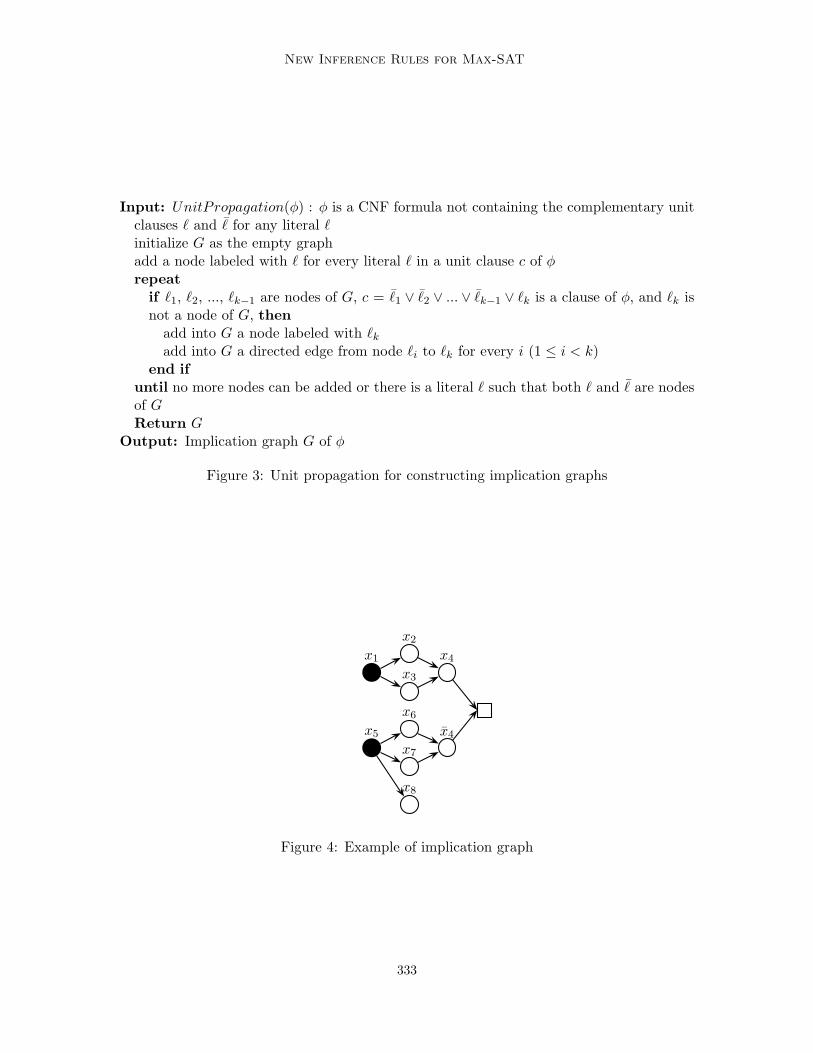
Given a CNF formula φ, Figure 3 shows how unit propagation constructs an implicationgraph whose nodes are literals.
Note that every node in G corresponds to a different literal, where ℓ and ℓ are consideredas different literals. When the CNF formula contains several copies of a unit clause ℓ, thealgorithm adds just one node with label ℓ.
Example 5 Let φ={x1, x1, x1∨x2, x1∨x3, x2∨x3∨x4, x5, x5∨x6, x5∨x7, x6∨x7∨x4, x5∨x8}.UnitPropagation constructs the implication graph of Figure 4, in which we add a specialnode 2 to highlight the contradiction.
G is always acyclic because every added edge connects a new node. It is well knownthat the time complexity of unit propagation is O(|φ|), where |φ| is the size of φ (see, e.g.,Freeman, 1995).
We associate clause c=ℓ1∨ℓ2∨...∨ℓk−1∨ℓk with node ℓk if node ℓk is added into G becauseof c. Note that node ℓk does not have any incoming edge if and only if c is unit (k=1), andthe node has only one incoming edge if and only if c is binary (k=2). Once G is constructed,if G contains both ℓ and ℓ for some literal ℓ (i.e., unit propagation deduces a contradiction),it is easy to identify all nodes from which there exists a path to ℓ or ℓ in G; i.e., the clauses
332
New Inference Rules for Max-SAT
Input: UnitPropagation(φ) : φ is a CNF formula not containing the complementary unitclauses ℓ and ℓ for any literal ℓ
initialize G as the empty graphadd a node labeled with ℓ for every literal ℓ in a unit clause c of φ
repeatif ℓ1, ℓ2, ..., ℓk−1 are nodes of G, c = ℓ1 ∨ ℓ2 ∨ ... ∨ ℓk−1 ∨ ℓk is a clause of φ, and ℓk isnot a node of G, then
add into G a node labeled with ℓk
add into G a directed edge from node ℓi to ℓk for every i (1 ≤ i < k)end if
until no more nodes can be added or there is a literal ℓ such that both ℓ and ℓ are nodesof G
Return G
Output: Implication graph G of φ
Figure 3: Unit propagation for constructing implication graphs
x1
x2
x3
x4
x5
x6
x7
x4
x8
Figure 4: Example of implication graph
333
Li, Manya & Planes
c1 c2 c3 c4
c5 c6 c7
x1 x2 x3 x4
x5 x6 x4
Figure 5: Example of implication graph
implying ℓ or ℓ. All these clauses constitute an inconsistent subset S of φ. In the aboveexample, clauses x1, x1∨x2, x1∨x3 and x2∨ x3∨x4 imply x4, and clauses x5, x5∨x6, x5∨x7
and x6 ∨ x7 ∨ x4 imply x4. Clause x5 ∨ x8 does not contribute to the contradiction. Theinconsistent subset S is {x1, x1 ∨ x2, x1 ∨ x3, x2 ∨ x3 ∨ x4, x5, x5 ∨ x6, x5 ∨ x7, x6 ∨ x7 ∨ x4}.
5.2 Applicability of Rule 3, Rule 4, Rule 5, and Rule 6
We assume that unit propagation deduces a contradiction and, therefore, the implicationgraph G contains both ℓ and ℓ for some literal ℓ. Let Sℓ be the set of all nodes from whichthere exists a path to ℓ, let Sℓ be the set of all nodes from which there exists a path toℓ, and let S=Sℓ ∪ Sℓ. As a clause is associated with each node in G, we also use S, Sℓ,and Sℓ to denote the set of clauses associated with the nodes in S, Sℓ, and Sℓ, respectively.Lemma 2 and Lemma 3 are used to detect the applicability of Rule 3, Rule 4, Rule 5, andRule 6.
Lemma 2 Rule 3 and Rule 4 are applicable if
1. in Sℓ (resp. Sℓ), there is one unit clause and all the other clauses are binary,
2. nodes in Sℓ (resp. Sℓ) form an implication chain starting at the unit clause and endingat ℓ (resp. ℓ),
3. Sℓ ∩ Sℓ is empty.
Proof 8 Starting from the node corresponding to the unit clause in Sℓ (resp. Sℓ), andfollowing in parallel the two implication chains, we have φ1 in Rule 3 or Rule 4 by writingdown the clause corresponding to each node. �
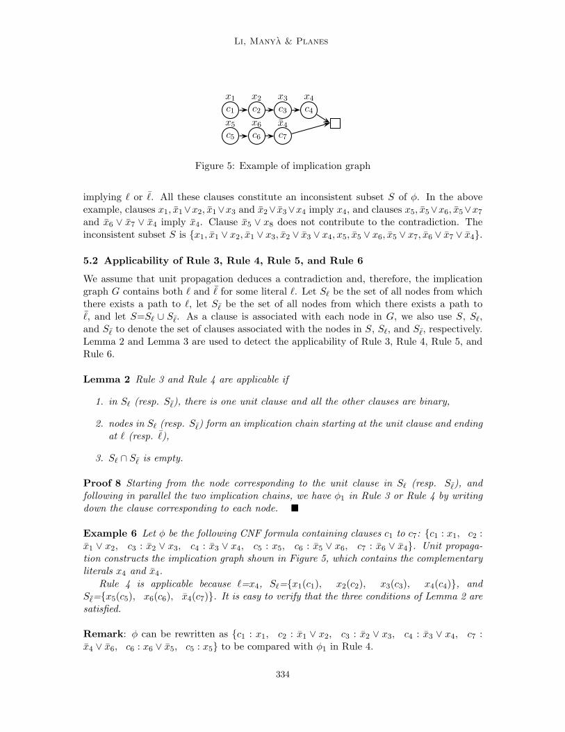
Example 6 Let φ be the following CNF formula containing clauses c1 to c7: {c1 : x1, c2 :x1 ∨ x2, c3 : x2 ∨ x3, c4 : x3 ∨ x4, c5 : x5, c6 : x5 ∨ x6, c7 : x6 ∨ x4}. Unit propaga-tion constructs the implication graph shown in Figure 5, which contains the complementaryliterals x4 and x4.
Rule 4 is applicable because ℓ=x4, Sℓ={x1(c1), x2(c2), x3(c3), x4(c4)}, andSℓ={x5(c5), x6(c6), x4(c7)}. It is easy to verify that the three conditions of Lemma 2 aresatisfied.
Remark: φ can be rewritten as {c1 : x1, c2 : x1 ∨ x2, c3 : x2 ∨ x3, c4 : x3 ∨ x4, c7 :x4 ∨ x6, c6 : x6 ∨ x5, c5 : x5} to be compared with φ1 in Rule 4.
334
New Inference Rules for Max-SAT
c1 c2 c3
c4
c5
x1 x2 x3 x4
x4
Figure 6: Example of implication graph
The application of Rule 3 and Rule 4 consists of replacing every binary clause c in S
with a binary clause obtained by negating every literal of c, removing the two unit clausesof S from φ, and incrementing #emptyClauses(φ) by 1.
Lemma 3 Rule 5 and Rule 6 are applicable if
1. in S=Sℓ ∪ Sℓ, there is one unit clause and all the other clauses are binary; i.e., allnodes in S, except for the node corresponding to the unit clause, have exactly oneincoming edge in G.
2. Sℓ ∩ Sℓ is non-empty and contains k (k >0) nodes forming an implication chain ofthe form ℓ1 → ℓ2 → · · · → ℓk, where ℓk is the last node of the chain.
3. (Sℓ ∪ Sℓ)-(Sℓ ∩ Sℓ) contains exactly three nodes : ℓ, ℓ, and a third one. Let ℓk+1 bethe third literal,
if ℓk+1 ∈ Sℓ, then G contains the following implications
ℓk → ℓk+1 → ℓ
ℓk → ℓ
if ℓk+1 ∈ Sℓ, then G contains the following implications
ℓk → ℓ
ℓk → ℓk+1 → ℓ
Proof 9 Assume, without loss of generality, that ℓk+1 ∈ Sℓ; the case ℓk+1 ∈ Sℓ is symmet-ric. The implication chain formed by the nodes of Sℓ ∩ Sℓ corresponds to the clauses {ℓ1,ℓ1 ∨ ℓ2, . . . , ℓk−1 ∨ ℓk}, which, together with the three clauses {ℓk ∨ ℓk+1, ℓk+1 ∨ ℓ, ℓk ∨ ℓ}corresponding to ℓk → ℓk+1 → ℓ and ℓk → ℓ, give φ1 in Rule 5 or Rule 6. �
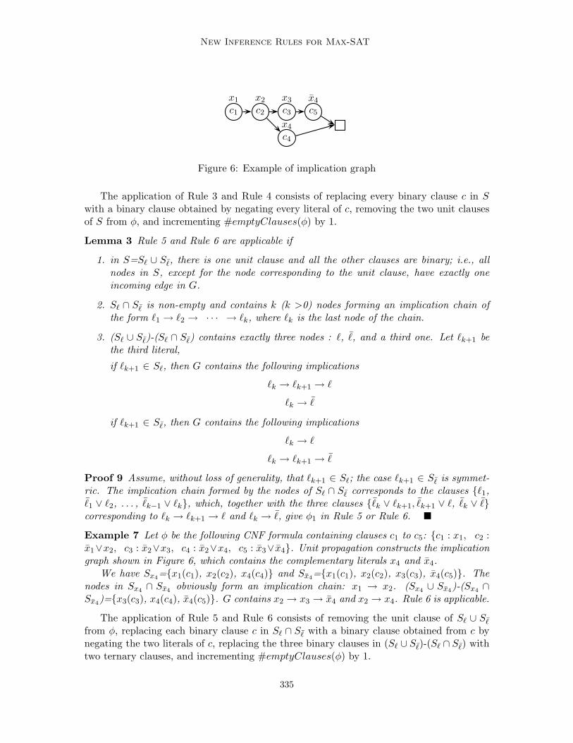
Example 7 Let φ be the following CNF formula containing clauses c1 to c5: {c1 : x1, c2 :x1∨x2, c3 : x2∨x3, c4 : x2∨x4, c5 : x3∨ x4}. Unit propagation constructs the implicationgraph shown in Figure 6, which contains the complementary literals x4 and x4.
We have Sx4={x1(c1), x2(c2), x4(c4)} and Sx4
={x1(c1), x2(c2), x3(c3), x4(c5)}. Thenodes in Sx4
∩ Sx4obviously form an implication chain: x1 → x2. (Sx4
∪ Sx4)-(Sx4
∩Sx4
)={x3(c3), x4(c4), x4(c5)}. G contains x2 → x3 → x4 and x2 → x4. Rule 6 is applicable.
The application of Rule 5 and Rule 6 consists of removing the unit clause of Sℓ ∪ Sℓ
from φ, replacing each binary clause c in Sℓ ∩ Sℓ with a binary clause obtained from c bynegating the two literals of c, replacing the three binary clauses in (Sℓ ∪ Sℓ)-(Sℓ ∩ Sℓ) withtwo ternary clauses, and incrementing #emptyClauses(φ) by 1.
335
Li, Manya & Planes
5.3 Complexity, Termination, and (In)Completeness of Rule Applications
In our branch and bound algorithm for Max-SAT, we combine the application of the infer-ence rules and the computation of the underestimation of the lower bound. Given a CNFformula φ, function underestimation uses unit propagation to construct an implicationgraph G. Once G contains two nodes ℓ and ℓ for some literal ℓ, G is analyzed to determinewhether some inference rule is applicable. If some rule is applicable, it is applied and φ istransformed into an equivalent Max-SAT instance. Otherwise, all clauses contributing tothe contradiction are removed from φ, and the underestimation is incremented by 1. Thisprocedure is repeated until unit propagation cannot derive more contradictions. Finally, allremoved clauses, except those removed or replaced due to inference rule applications, arereinserted into φ. The underestimation, together with the new φ, is returned.
It is well known that unit propagation can be implemented with a time complexity linearin the size of φ (see, e.g., Freeman, 1995). The complexity of determining the applicabilityof the inference rules using Lemma 2 and Lemma 3 is linear in the size of G, bounded bythe number of literals in φ, if we assume that the graph is represented by doubly-linkedlists. The application of an inference rule is obviously linear in the size of G. So, the wholetime complexity of function underestimation with inference rule applications is O(d ∗ |φ|),where d is the number of contradictions that function underestimation is able to detectusing unit propagation. Observe that the factor d is needed because the application of therules inserts new clauses in the place of the removed clauses.
Since every inference rule application reduces the size of φ, function underestimation
with inference rule applications has linear space complexity, and it always terminates. Recallthat new clauses added by the inference rules can be stored in the place of the old ones.The data structures for loading φ can be statically and efficiently maintained.
We have proved that the inference rules are sound. The following example shows thatthe application of the rules is not necessarily complete in our implementation, in the sensethat not all possible applications of the inference rules are necessarily done.
Example 8 Let φ={x1, x3, x4, x1 ∨ x3 ∨ x4, x1 ∨ x2, x2}. Unit propagation may discoverthe inconsistent subset S={x1, x3, x4, x1 ∨ x3 ∨ x4}. In this case, no inference rule is ap-plicable to S. Then, the underestimation of the lower bound is incremented by 1, and φ
becomes {x1 ∨ x2, x2}. Unit propagation cannot detect more contradictions in φ, and func-tion underestimation stops after reinserting {x1, x3, x4, x1 ∨ x3 ∨ x4} into φ. The value1 is returned, together with the unchanged φ. Note that Rule 3 is applicable to the subset{x1, x1 ∨ x2, x2} of φ, but is not applied.
Actually, function underestimation only applies Rule 3 if unit propagation detects theinconsistent subset {x1, x1 ∨ x2, x2} instead of {x1, x3, x4, x1 ∨ x3 ∨ x4}. The detection ofan inconsistent subset depends on the ordering in which unit clauses are propagated in unitpropagation. In this example, the inconsistent subset {x1, x1 ∨ x2, x2} is discovered if unitclause x2 is propagated before x3 and x4. Further study is needed to define orderings forunit clauses that maximize the application of inference rules.
Observe that our algorithm is deterministic, and always computes the same lower boundif the order of clauses is not changed.
336
New Inference Rules for Max-SAT
5.4 Inference Rules for Weighted Max-SAT
The inference rules presented in this paper can be naturally extended to weighted Max-SAT.In weighted Max-SAT, every clause is associated with a weight and the problem consistsof finding a truth assignment for which the sum of the weights of unsatisfied clauses isminimum. For example, the weighted version of Rule 3 could be
Rule 7 If φ1={(l1, w1), (l1 ∨ l2, w2), (l2, w3)}∪φ′, then φ2={(2, w), (l1 ∨ l2, w), (l1, w1−w), (l1 ∨ l2, w2 − w), (l2, w3 − w)} ∪ φ′ is equivalent to φ1
where w1, w2 and w3 are positive integers representing the clause weight, and w=min(w1,w2, w3). Mandatory clauses, that have to be satisfied in any optimal solution, are specifiedwith the weight ∞. Note that if w 6=∞, ∞-w=∞ and if w=∞, no optimal solution can befound and the solver should backtrack. Clauses with weight 0 are removed. Observe that φ1
can be rewritten as φ11 ∪ φ12, where φ11={(l1, w), (l1 ∨ l2, w), (l2, w)}, and φ12={(l1, w1 −w), (l1 ∨ l2, w2 −w), (l2, w3 −w)} ∪ φ′. Then, the weighted inference rule is equivalent tothe unweighted version applied w times to the (unweighted) clauses of φ11.
Similarly, the weighted version of Rule 4 could be
Rule 8 If φ1={(l1, w1) (l1 ∨ l2, w2), (l2 ∨ l3, w3), . . . , (lk ∨ lk+1, wk+1), (lk+1, wk+2)}∪φ′,then φ2={(2, w), (l1 ∨ l2, w), (l2 ∨ l3, w), . . . , (lk ∨ lk+1, w), (l1, w1 − w), (l1 ∨ l2, w2 −w), (l2 ∨ l3, w3 − w), . . . , (lk ∨ lk+1, wk+1 − w), (lk+1, wk+2 − w)} ∪ φ′ is equivalent to φ1
where w=min(w1, w2, . . . , wk+2). Observe that φ1 can also be rewritten as φ11 ∪ φ12, withφ11={(l1, w) (l1 ∨ l2, w), (l2 ∨ l3, w), . . . , (lk ∨ lk+1, w), (lk+1, w)}, The weighted version ofRule 4 is equivalent to the unweighted Rule 4 applied w times to the (unweighted) clausesof φ11.
The current implementation of the inference rules can be naturally extended to weightedinference rules. If an inconsistent subformula is detected and a rule is applicable (clauseweights are not considered in the detection of the inconsistent subformula and of the ap-plicability of the rule, provided that clauses with weight 0 have been discarded), then φ11
and φ12 are separated after computing the minimal weight w of all clauses in the detectedinconsistent subformula, and the rule is applied to φ11. The derived clauses and clauses inφ12 can be used in subsequent reasoning.
6. MaxSatz: a New Max-SAT Solver
We have implemented a new Max-SAT solver, called MaxSatz, that incorporates the lowerbound computation method based on unit propagation defined in Section 3, and applies theinference rules defined in Section 4. The name of MaxSatz comes from the fact that theimplementation of our algorithm incorporates most of the technology that was developedfor the SAT solver Satz (Li & Anbulagan, 1997b, 1997a).
MaxSatz incorporates the lower bound based on unit propagation, and applies Rule 1,Rule 2, Rule 3, Rule 4, Rule 5, and Rule 6. In addition, MaxSatz applies the followingtechniques:
• Pure literal rule: If a literal only appears with either positive polarity or negativepolarity, we delete the clauses containing that literal.
337

Li, Manya & Planes
• Empty-Unit clause rule (Alsinet et al., 2003a): Let neg1(x) (pos1(x)) be the number ofunit clauses in which x is negative (positive). If #emptyClauses(φ)+neg1(x) ≥ UB,then we assign x to false. If #emptyClauses(φ) + pos1(x) ≥ UB, then we assign x
to true.
• Dominating Unit Clause (DUC) rule (Niedermeier & Rossmanith, 2000): If the num-ber of clauses in which a literal x (x) appears is not greater than neg1(x) (pos1(x)),then we assign x to false (true).
• Variable selection heuristic: Let neg2(x) (pos2(x)) be the number of binary clausesin which x is negative (positive), and let neg3(x) (pos3(x)) be the number of clausescontaining three or more literals in which x is negative (positive). We select thevariable x such that (neg1(x)+4∗neg2(x)+neg3(x))*(pos1(x)+4∗pos2(x)+pos3(x))is the largest. The fact that binary clauses are counted four times more than otherclauses was determined empirically.
• Value selection heuristic: Let x be the selected branching variable. If neg1(x) + 4 ∗neg2(x) + neg3(x) < pos1(x) + 4 ∗ pos2(x) + pos3(x), set x to true. Otherwise set x
to false. This heuristics was also determined empirically.
In this paper, in order to compare the inference rules defined, we have used three sim-plified versions of MaxSatz:
• MaxSat0: does not apply any inference rule defined in Section 4.
• MaxSat12: applies rules 1 and 2, but not rules 3, 4, 5 and 6.
• MaxSat1234: applies rules 1, 2, 3 and 4, but not rules 5 and 6.
Actually, MaxSatz corresponds to MaxSat123456 in our terminology. MaxSat12 corre-sponds to an improved version of the solver UP (Li et al., 2005), using a special orderingfor propagating unit clauses in unit propagation. MaxSat12 maintains two queues duringunit propagation: Q1 and Q2. When MaxSat12 starts the search for an inconsistent sub-formula via unit propagation, Q1 contains all the unit clauses of the CNF formula underconsideration (more recently derived unit clauses are at the end of Q1), and Q2 is empty.The unit clauses derived during the application of unit propagation are stored in Q2, andunit propagation does not use any unit clause from Q1 unless Q2 is empty. Intuitively, thisordering prefers unit clauses which were non-unit clauses before starting the application ofunit propagation. This way, the derived inconsistent subset contains, in general, less unitclauses. The unit clauses which have not been consumed will contribute to detect furtherinconsistent subsets. Our experimental results (Li, Manya, & Planes, 2006) show that thesearch tree size of MaxSat12 is substantially smaller than that of UP, and MaxSat12 issubstantially faster than UP. MaxSat0, Maxsat1234, and MaxSatz use the same orderingas MaxSat12 for propagating unit clauses in unit propagation.
The source code of MaxSat0, MaxSat12, MaxSat1234, and MaxSatz can be found athttp://web.udl.es/usuaris/m4372594/jair-maxsatz-solvers.zip, and at http://www.laria.u-picardie.fr/˜cli/maxsatz.tar.gz.
338
New Inference Rules for Max-SAT
7. Experimental Results
We report on the experimental investigation performed for unweighted Max-SAT in orderto evaluate the inference rules defined in Section 4, and to compare MaxSatz with thebest performing state-of-the-art solvers that were publicly available when this paper wassubmitted. The experiments were performed on a Linux Cluster with processors 2 GHzAMD Opteron with 1 Gb of RAM.
The structure of this section is as follows. We first describe the solvers and benchmarksthat we have considered. Then, we present the experimental evaluation of the inferencerules. Finally, we show the experimental comparison of MaxSatz with other solvers.
7.1 Solvers and Benchmarks
MaxSatz was compared with the following Max-SAT solvers:
• BF2 (Borchers & Furman, 1999): a branch and bound Max-SAT solver which usesMOMS as dynamic variable selection heuristic and does not consider underestimationsin the computation of the lower bound. It was developed by Borchers and Furman in1999.
• AGN3 (Alber et al., 2001): a branch and bound Max-2SAT solver. It was developedby Alber, Gramm and Niedermeier in 1998.
• AMP4 (Alsinet et al., 2003b): a branch and bound Max-SAT solver based on BF thatincorporates a lower bound of better quality and the Jeroslow-Wang variable selectionheuristic (Jeroslow & Wang, 1990). It was developed by Alsinet, Manya and Planesand presented at SAT-2003.
• toolbar5 (de Givry et al., 2003; Larrosa & Heras, 2005): a Max-SAT solver whoseinference was inspired in soft arc consistency properties implemented in weighted CSPsolvers. It was developed by de Givry, Larrosa, Meseguer and Schiex and was firstpresented at CP-2003. We used version 2.2 with default parameters.
• MaxSolver6 (Xing & Zhang, 2004): a branch and bound Max-SAT solver that applies anumber of efficient inference rules. It was developed by Xing and Zhang and presentedat CP-2004. We used the second release of this solver.
• Lazy7 (Alsinet et al., 2005): a branch and bound Max-SAT solver with lazy datastructures and a static variable selection heuristic. It was developed by Alsinet, Manyaand Planes and presented at SAT-2005.
2. Downloaded in October 2004 from http://infohost.nmt.edu/˜borchers/satcodes.tar.gz3. Downloaded in October 2005 from http://www-fs.informatik.uni-tuebingen.de/˜gramm/4. Available at http://web.udl.es/usuaris/m4372594/software.html5. Downloaded in October 2005 from http://carlit.toulouse.inra.fr/cgi-bin/awki.cgi/ToolBarIntro6. Downloaded in October 2005 from http://cic.cs.wustl.edu/maxsolver/7. Available at http://web.udl.es/usuaris/m4372594/software.html
339
Li, Manya & Planes
• UP8 (Li et al., 2005): a branch and bound Max-SAT solver with the lower boundcomputation method based on unit propagation (cf. Section 3). It was developed byLi, Manya and Planes and presented at CP-2005.
We used as benchmarks randomly generated Max-2SAT instances and Max-3SAT in-stances, graph 3-coloring instances9, as well as Max-Cut instances10. We also considered theunweighted Max-SAT benchmarks submitted to the Max-SAT Evaluation 2006, includingMax-Cut, Max-Ones, Ramsey numbers, and random Max-2SAT and Max-3SAT instances.
We generated Max-2SAT instances and Max-3SAT instances using the generator mwff.cdeveloped by Bart Selman, which allows for duplicated clauses. For Max-Cut, we firstgenerated a random graph of m edges in which every edge is randomly selected amongthe set of all possible edges. If the graph is not connected, it is discarded. If the graphis connected, we used the encoding of Shen and Zhang (2005) to encode the Max-Cutinstance into a CNF: we created, for each edge (xi, xj), exactly two binary clauses (xi ∨xj)and (xi ∨ xj). If φ is the collection of such binary clauses, then the Max-Cut instance hasa cut of weight k iff the Max-SAT instance has an assignment under which m + k clausesare satisfied.
For graph 3-coloring, we first used Culberson’s generator to generate a random k-colorable graph of type IID (independent random edge assignment, variability=0) withk vertices and a fixed edge density. We then used Culberson’s converter to SAT with stan-dard conversion and three colors to generate a Max-SAT instance: for each vertex xi andfor each color j ∈ {1, 2, 3}, a propositional variable xij is defined meaning that vertex i iscolored with color j. For each vertex xi, four clauses are added to encode that the vertexis colored with exactly one color: xi1 ∨ xi2 ∨ xi3, xi1 ∨ xi2, xi1 ∨ xi3, and xi2 ∨ xi3; and, foreach edge (xi, xj), three clauses are added to encode that vertex xi and vertex xj do nothave the same color: xi1 ∨ xj1, xi2 ∨ xj2, and xi3 ∨ xj3.
In random Max-2SAT and Max-3SAT instances, clauses are entirely independent to eachother and do not have structure. In the graph 3-coloring instances and Max-Cut instancesused in this paper, clauses are not independent and have structure. For example, in aMax-Cut instance, every time we have a clause xi ∨ xj , we also have the clause xi ∨ xj ;the satisfaction of these two clauses means that the corresponding edge is in the cut. In agraph 3-coloring instance, every time we have a ternary clause xi1 ∨ xi2 ∨ xi3 encoding thatvertex i is colored with at least a color, we also have three binary clauses xi1∨ xi2, xi1∨ xi3,and xi2 ∨ xi3 encoding that vertex i cannot be colored with two or more colors. Max-Cut instances only contain binary clauses, but graph 3-coloring instances contain a ternaryclause for every vertex in the graph. While we can derive an optimal cut from an optimalassignment of a Max-SAT encoding of any Max-Cut instance, an optimal assignment of aMax-SAT encoding of a 3-coloring instance may assign more than one color to some vertices.
8. Available at http://web.udl.es/usuaris/m4372594/software.html9. Given an undirected graph G = (V, E), where V = {x1, . . . , xn} is the set of vertices and E is the set
of edges, and a set of three colors, the graph 3-coloring problem is the problem of coloring every vertexwith one of the three colors in such a way that, for each edge (xi, xj) ∈ E, vertex xi and vertex xj donot have the same color.
10. Given an undirected graph G = (V, E), let wxi,xjbe the weight associated with each edge (xi, xj) ∈ E.
The weighted Max-Cut problem is to find a subset S of V such that W (S, S) =P
xi∈S,xj∈Swxi,xj
is
maximized, where S = V − S. In this paper, we set weight wxi,xj= 1 for all edges.
340
New Inference Rules for Max-SAT
The Max-Cut and Ramsey numbers instances from the Max-SAT Evaluation 2006 con-tain different structures. For example, the underlying graphs in the Max-Cut instanceshave different origins such as fault diagnosis problems, coding theory problems, and graphclique problems. Max-2SAT and Max-3SAT instances from the evaluation do not containduplicated clauses.
We computed an initial upper bound with a local search solver for each instance. Wedid not provide any parameter to any solver except the instance to be solved and the initialupper bound. In other words, we used the default values for all the parameters. Theinstances from the Max-SAT Evaluation 2006 were solved in the same conditions as in theevaluation; i.e., no initial upper bound was provided to the solvers, and the maximum timeallowed to solve an instance was 30 minutes.
7.2 Evaluation of the Inference Rules
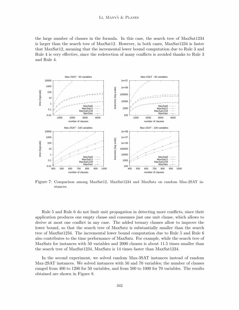
In the first experiment performed to evaluate the impact of the inference rules of Section 4,we solved sets of 100 random Max-2SAT instances with 50 and 100 variables; the numberof clauses ranged from 400 to 4500 for 50 variables, and from 400 to 1000 for 100 variables.The results obtained are shown in Figure 7. Along the horizontal axis is the number ofclauses, and along the vertical axis is the mean time (left plot), in seconds, needed to solvean instance of a set, and the mean number of branches of the proof tree (right plot). Noticethat we use a log scale to represent both run-time and branches.
We observe that the rules are very powerful for Max-2SAT and the gain increases asthe number of variables and the number of clauses increase. For 50 variables and 1000clauses (the clause to variable ratio is 20), MaxSatz is 7.6 times faster than MaxSat1234;and for 100 variables and 1000 clauses (the clause to variable ratio is 10), MaxSatz is 9.2times faster than MaxSat1234. The search tree of MaxSatz is also substantially smallerthan that of MaxSat1234. Rule 5 and Rule 6 are more powerful than Rule 3 and Rule 4 forMax-2SAT. The intuitive explanation is that MaxSatz and MaxSat1234 detect many moreinconsistent subsets of clauses containing one unit clause than subsets containing two unitclauses, so that Rule 5 and Rule 6 can be applied many more times than Rule 3 and Rule 4in MaxSatz.
Recall that, on the one hand, every application of Rule 3 and Rule 4 consumes twounit clauses but only produces one empty clause, limiting unit propagation in detectingmore conflicts in subsequent search. On the other hand, Rule 3 and Rule 4 add clauseswhich may contribute to detect further conflicts. Depending on the number of clauses (ormore precisely, the clause to variable ratio) in a formula, these two factors have differentimportance. When there are relatively few clauses, unit propagation relatively does noteasily derive a contradiction from a unit clause, and the binary clauses added by Rule 3 andRule 4 are relatively important for deriving additional conflicts and improving the lowerbound, which explains why the search tree of MaxSat1234 is smaller than the search treeof MaxSat12 for instances with 100 variables and less than 600 clauses. On the contrary,when there are many clauses, unit propagation easily derives a contradiction from a unitclause, so that the two unit clauses consumed by Rule 3 and Rule 4 would probably allow toderive two disjoint inconsistent subsets of clauses. In addition, the binary clauses added byRule 3 and Rule 4 are relatively less important for deriving additional conflicts, considering
341
Li, Manya & Planes
the large number of clauses in the formula. In this case, the search tree of MaxSat1234is larger than the search tree of MaxSat12. However, in both cases, MaxSat1234 is fasterthat MaxSat12, meaning that the incremental lower bound computation due to Rule 3 andRule 4 is very effective, since the redetection of many conflicts is avoided thanks to Rule 3and Rule 4.
0.01
0.1
1
10
100
1000
10000
1000 2000 3000 4000
time
(logs
cale
)
number of clauses
Max-2SAT - 50 variables
MaxSat0MaxSat12
MaxSat1234MaxSatz
100
1000
10000
100000
1e+06
1e+07
1000 2000 3000 4000br
anch
es (
log
scal
e)
number of clauses
Max-2SAT - 50 variables
MaxSat0MaxSat12
MaxSat1234MaxSatz
0.01
0.1
1
10
100
1000
10000
400 500 600 700 800 900 1000
time
(logs
cale
)
number of clauses
Max-2SAT - 100 variables
MaxSat0MaxSat12
MaxSat1234MaxSatz
100
1000
10000
100000
1e+06
1e+07
1e+08
400 500 600 700 800 900 1000
bran
ches
(lo
g sc
ale)
number of clauses
Max-2SAT - 100 variables
MaxSat0MaxSat12
MaxSat1234MaxSatz
Figure 7: Comparison among MaxSat12, MaxSat1234 and MaxSatz on random Max-2SAT in-stances.
Rule 5 and Rule 6 do not limit unit propagation in detecting more conflicts, since theirapplication produces one empty clause and consumes just one unit clause, which allows toderive at most one conflict in any case. The added ternary clauses allow to improve thelower bound, so that the search tree of MaxSatz is substantially smaller than the searchtree of MaxSat1234. The incremental lower bound computation due to Rule 5 and Rule 6also contributes to the time performance of MaxSatz. For example, while the search tree ofMaxSatz for instances with 50 variables and 2000 clauses is about 11.5 times smaller thanthe search tree of MaxSat1234, MaxSatz is 14 times faster than MaxSat1234.
In the second experiment, we solved random Max-3SAT instances instead of randomMax-2SAT instances. We solved instances with 50 and 70 variables; the number of clausesranged from 400 to 1200 for 50 variables, and from 500 to 1000 for 70 variables. The resultsobtained are shown in Figure 8.
342
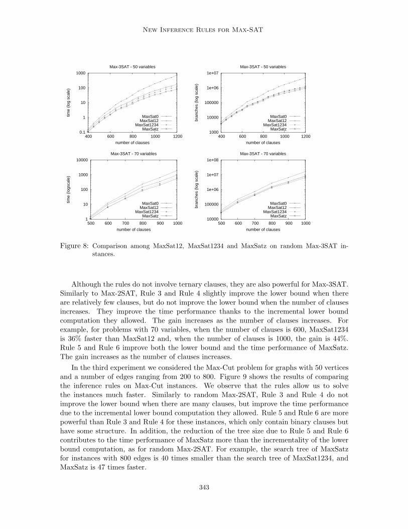
New Inference Rules for Max-SAT
0.1
1
10
100
1000
400 600 800 1000 1200
time
(log
scal
e)
number of clauses
Max-3SAT - 50 variables
MaxSat0MaxSat12
MaxSat1234MaxSatz
1000
10000
100000
1e+06
1e+07
400 600 800 1000 1200
bran
ches
(lo
g sc
ale)
number of clauses
Max-3SAT - 50 variables
MaxSat0MaxSat12
MaxSat1234MaxSatz
1
10
100
1000
10000
500 600 700 800 900 1000
time
(logs
cale
)
number of clauses
Max-3SAT - 70 variables
MaxSat0MaxSat12
MaxSat1234MaxSatz
10000
100000
1e+06
1e+07
1e+08
500 600 700 800 900 1000
bran
ches
(lo
g sc
ale)
number of clauses
Max-3SAT - 70 variables
MaxSat0MaxSat12
MaxSat1234MaxSatz
Figure 8: Comparison among MaxSat12, MaxSat1234 and MaxSatz on random Max-3SAT in-stances.
Although the rules do not involve ternary clauses, they are also powerful for Max-3SAT.Similarly to Max-2SAT, Rule 3 and Rule 4 slightly improve the lower bound when thereare relatively few clauses, but do not improve the lower bound when the number of clausesincreases. They improve the time performance thanks to the incremental lower boundcomputation they allowed. The gain increases as the number of clauses increases. Forexample, for problems with 70 variables, when the number of clauses is 600, MaxSat1234is 36% faster than MaxSat12 and, when the number of clauses is 1000, the gain is 44%.Rule 5 and Rule 6 improve both the lower bound and the time performance of MaxSatz.The gain increases as the number of clauses increases.
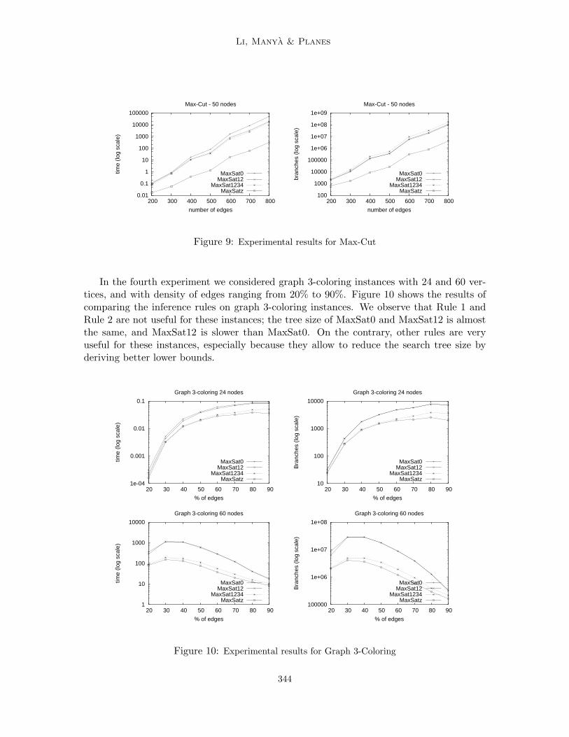
In the third experiment we considered the Max-Cut problem for graphs with 50 verticesand a number of edges ranging from 200 to 800. Figure 9 shows the results of comparingthe inference rules on Max-Cut instances. We observe that the rules allow us to solvethe instances much faster. Similarly to random Max-2SAT, Rule 3 and Rule 4 do notimprove the lower bound when there are many clauses, but improve the time performancedue to the incremental lower bound computation they allowed. Rule 5 and Rule 6 are morepowerful than Rule 3 and Rule 4 for these instances, which only contain binary clauses buthave some structure. In addition, the reduction of the tree size due to Rule 5 and Rule 6contributes to the time performance of MaxSatz more than the incrementality of the lowerbound computation, as for random Max-2SAT. For example, the search tree of MaxSatzfor instances with 800 edges is 40 times smaller than the search tree of MaxSat1234, andMaxSatz is 47 times faster.
343
Li, Manya & Planes
0.01
0.1
1
10
100
1000
10000
100000
200 300 400 500 600 700 800
time
(log
scal
e)
number of edges
Max-Cut - 50 nodes
MaxSat0MaxSat12
MaxSat1234MaxSatz
100
1000
10000
100000
1e+06
1e+07
1e+08
1e+09
200 300 400 500 600 700 800
bran
ches
(lo
g sc
ale)
number of edges
Max-Cut - 50 nodes
MaxSat0MaxSat12
MaxSat1234MaxSatz
Figure 9: Experimental results for Max-Cut
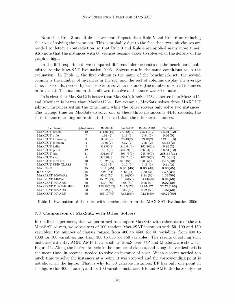
In the fourth experiment we considered graph 3-coloring instances with 24 and 60 ver-tices, and with density of edges ranging from 20% to 90%. Figure 10 shows the results ofcomparing the inference rules on graph 3-coloring instances. We observe that Rule 1 andRule 2 are not useful for these instances; the tree size of MaxSat0 and MaxSat12 is almostthe same, and MaxSat12 is slower than MaxSat0. On the contrary, other rules are veryuseful for these instances, especially because they allow to reduce the search tree size byderiving better lower bounds.
1e-04
0.001
0.01
0.1
20 30 40 50 60 70 80 90
time
(log
scal
e)
% of edges
Graph 3-coloring 24 nodes
MaxSat0MaxSat12
MaxSat1234MaxSatz
10
100
1000
10000
20 30 40 50 60 70 80 90
Bra
nche
s (lo
g sc
ale)
% of edges
Graph 3-coloring 24 nodes
MaxSat0MaxSat12
MaxSat1234MaxSatz
1
10
100
1000
10000
20 30 40 50 60 70 80 90
time
(log
scal
e)
% of edges
Graph 3-coloring 60 nodes
MaxSat0MaxSat12
MaxSat1234MaxSatz
100000
1e+06
1e+07
1e+08
20 30 40 50 60 70 80 90
Bra
nche
s (lo
g sc
ale)
% of edges
Graph 3-coloring 60 nodes
MaxSat0MaxSat12
MaxSat1234MaxSatz
Figure 10: Experimental results for Graph 3-Coloring
344
New Inference Rules for Max-SAT
Note that Rule 3 and Rule 4 have more impact than Rule 5 and Rule 6 on reducingthe cost of solving the instances. This is probably due to the fact that two unit clauses areneeded to detect a contradiction, so that Rule 3 and Rule 4 are applied many more times.Also note that the instances with 60 vertices become easier to solve when the density of thegraph is high.
In the fifth experiment, we compared different inference rules on the benchmarks sub-mitted to the Max-SAT Evaluation 2006. Solvers ran in the same conditions as in theevaluation. In Table 1, the first column is the name of the benchmark set, the secondcolumn is the number of instances in the set, and the rest of columns display the averagetime, in seconds, needed by each solver to solve an instance (the number of solved instancesin brackets). The maximum time allowed to solve an instance was 30 minutes.
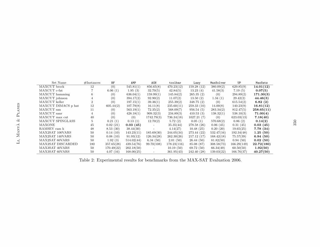
In is clear that MaxSat12 is better than MaxSat0, MaxSat1234 is better than MaxSat12,and MaxSatz is better than MaxSat1234. For example, MaxSatz solves three MAXCUTjohnson instances within the time limit, while the other solvers only solve two instances.The average time for MaxSatz to solve one of these three instances is 44.46 seconds, thethird instance needing more time to be solved than the other two instances.
Set Name #Instances MaxSat0 MaxSat12 MaxSat1234 MaxSatz
MAXCUT brock 12 471.01(10) 277.12(12) 225.11(12) 14.01(12)MAXCUT c-fat 7 1.92 (5) 3.11 (5) 2.84 (5) 0.07(5)MAXCUT hamming 6 39.42(2) 29.43(2) 29.48(2) 171.30(3)MAXCUT johnson 4 14.91(2) 8.57 (2) 7.21 (2) 44.46(3)MAXCUT keller 2 512.66(2) 213.64(2) 163.26(2) 6.82(2)MAXCUT p hat 12 72.16(9) 286.09(12) 226.24(12) 16.81(12)MAXCUT san 11 801.95(7) 305.75(7) 245.70(7) 258.65(11)MAXCUT sanr 4 323.67(3) 134.74(3) 107.76(3) 71.00(4)MAXCUT max cut 40 610.28(35) 481.48(40) 450.05(40) 7.18(40)MAXCUT SPINGLASS 5 0.22 (2) 0.19 (2) 0.15 (2) 0.14(2)MAXONE 45 0.03 (45) 0.03 (45) 0.03 (45) 0.03(45)RAMSEY 48 8.93 (34) 8.42 (34) 7.80 (34) 7.78(34)MAX2SAT 100VARS 50 95.01(50) 11.30(50) 8.14 (50) 1.25(50)MAX2SAT 140VARS 50 153.28(49) 51.76(50) 34.14(50) 6.94(50)MAX2SAT 60VARS 50 1.35 (50) 0.08 (50) 0.06 (50) 0.02(50)MAX2SAT DISCARDED 180 126.98(162) 71.85(173) 68.97(175) 22.72(180)MAX3SAT 40VARS 50 11.52(50) 3.33 (50) 2.52 (50) 1.92(50)MAX3SAT 60VARS 50 167.17(50) 72.72(50) 52.14(50) 40.27(50)
Table 1: Evaluation of the rules with benchmarks from the MAX-SAT Evaluation 2006.
7.3 Comparison of MaxSatz with Other Solvers
In the first experiment, that we performed to compare MaxSatz with other state-of-the-artMax-SAT solvers, we solved sets of 100 random Max-2SAT instances with 50, 100 and 150variables; the number of clauses ranged from 400 to 4500 for 50 variables, from 400 to1000 for 100 variables, and from 300 to 650 for 150 variables. The results of solving suchinstances with BF, AGN, AMP, Lazy, toolbar, MaxSolver, UP and MaxSatz are shown inFigure 11. Along the horizontal axis is the number of clauses, and along the vertical axis isthe mean time, in seconds, needed to solve an instance of a set. When a solver needed toomuch time to solve the instances at a point, it was stopped and the corresponding point isnot shown in the figure. That is why for 50 variable instances, BF has only one point inthe figure (for 400 clauses); and for 100 variable instances, BF and AMP also have only one
345
Li, Manya & Planes
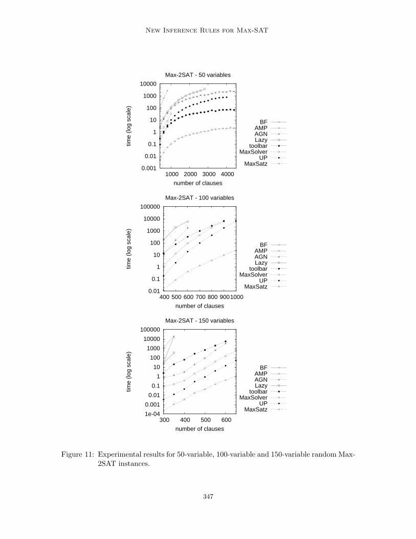
point in the figure (for 400 clauses). The version of MaxSolver we used limits the numberof clauses to 1000 in the instances to be solved. We ran it for instances up to 1000 clauses.
We see dramatic differences on performance between MaxSatz and the rest of solversin Figure 11. For the hardest instances, MaxSatz is up to two orders of magnitude fasterthan the second best performing solvers (UP). For those instances, MaxSatz needs 1 secondto solve an instance while solvers like MaxSolver and toolbar are not able to solve theseinstances after 10,000 seconds.
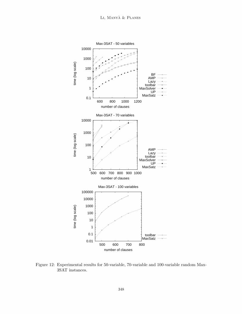
In the second experiment, we solved random Max-3SAT instances instead of randomMax-2SAT instances. The results obtained are shown in Figure 12. We did not considerAGN because it can only solve Max-2SAT instances. We solved instances with 50, 70 and100 variables; the number of clauses ranged from 500 to 1200 for 50 variables, from 500to 1000 for 70 variables, and from 450 to 800 for 100 variables. For 70 variables, AMPhas only one point in the figure (for 500 clauses) and BF is too slow. For 100 variables,we compared only the two best solvers. Once again, we observe dramatic differences onthe performance profile of MaxSatz and the rest of solvers. Particularly remarkable arethe differences between MaxSatz and toolbar (the second best performing solver on Max-3SAT), where we see that MaxSatz is up to 1,000 times faster than toolbar on the hardestinstances.
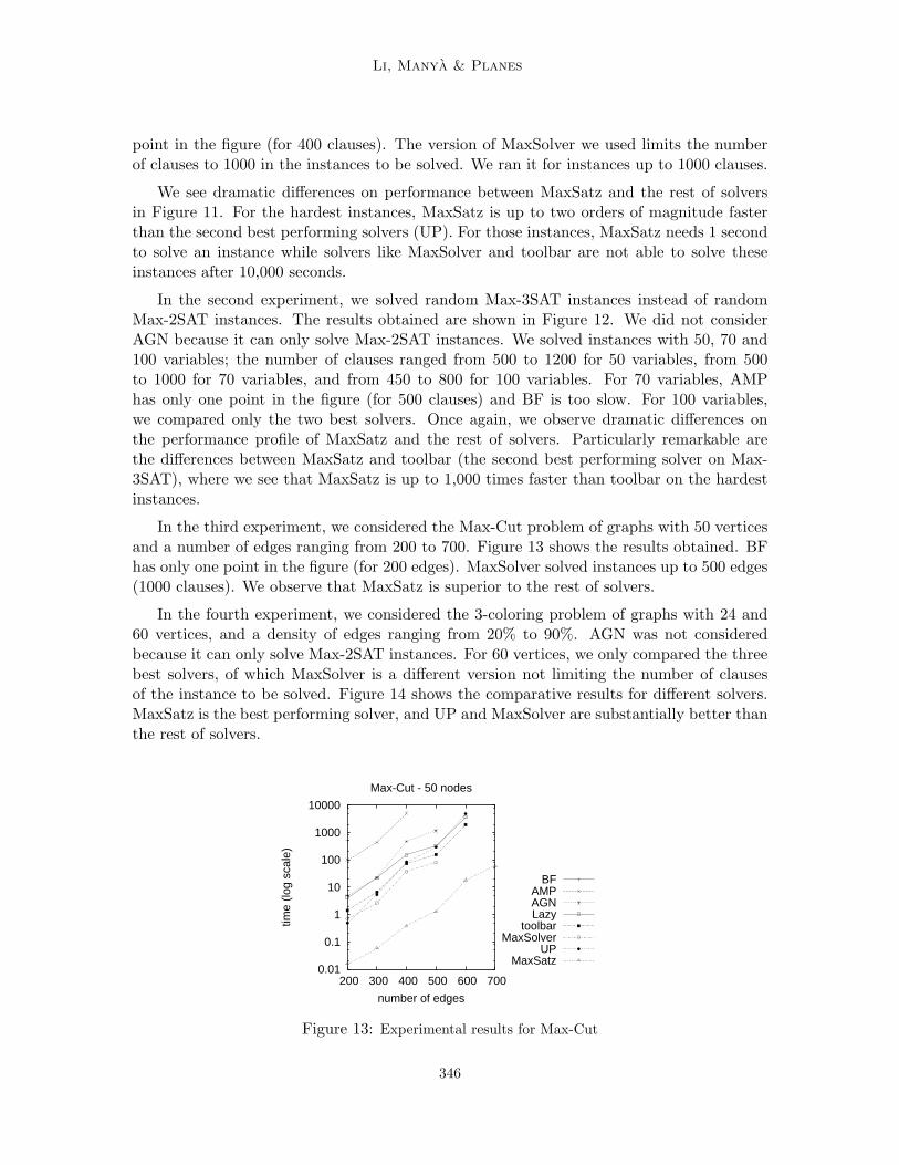
In the third experiment, we considered the Max-Cut problem of graphs with 50 verticesand a number of edges ranging from 200 to 700. Figure 13 shows the results obtained. BFhas only one point in the figure (for 200 edges). MaxSolver solved instances up to 500 edges(1000 clauses). We observe that MaxSatz is superior to the rest of solvers.
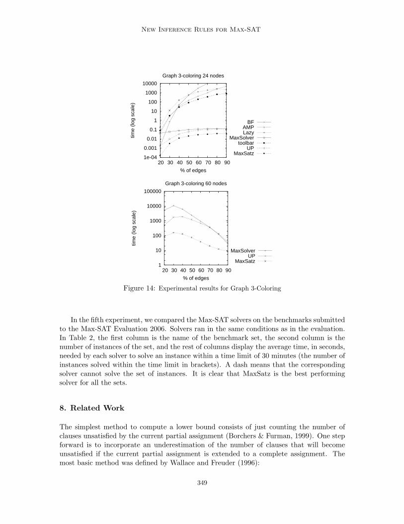
In the fourth experiment, we considered the 3-coloring problem of graphs with 24 and60 vertices, and a density of edges ranging from 20% to 90%. AGN was not consideredbecause it can only solve Max-2SAT instances. For 60 vertices, we only compared the threebest solvers, of which MaxSolver is a different version not limiting the number of clausesof the instance to be solved. Figure 14 shows the comparative results for different solvers.MaxSatz is the best performing solver, and UP and MaxSolver are substantially better thanthe rest of solvers.
0.01
0.1
1
10
100
1000
10000
200 300 400 500 600 700
time
(log
scal
e)
number of edges
Max-Cut - 50 nodes
BFAMPAGNLazy
toolbarMaxSolver
UPMaxSatz
Figure 13: Experimental results for Max-Cut
346
New Inference Rules for Max-SAT
0.001
0.01
0.1
1
10
100
1000
10000
1000 2000 3000 4000
time
(log
scal
e)
number of clauses
Max-2SAT - 50 variables
BFAMPAGNLazy
toolbarMaxSolver
UPMaxSatz
0.01
0.1
1
10
100
1000
10000
100000
400 500 600 700 800 900 1000
time
(log
scal
e)
number of clauses
Max-2SAT - 100 variables
BFAMPAGNLazy
toolbarMaxSolver
UPMaxSatz
1e-04
0.001
0.01
0.1
1
10
100
1000
10000
100000
300 400 500 600
time
(log
scal
e)
number of clauses
Max-2SAT - 150 variables
BFAMPAGNLazy
toolbarMaxSolver
UPMaxSatz
Figure 11: Experimental results for 50-variable, 100-variable and 150-variable random Max-2SAT instances.
347
Li, Manya & Planes
0.1
1
10
100
1000
10000
600 800 1000 1200
time
(log
scal
e)
number of clauses
Max-3SAT - 50 variables
BFAMPLazy
toolbarMaxSolver
UPMaxSatz
1
10
100
1000
10000
500 600 700 800 900 1000
time
(log
scal
e)
number of clauses
Max-3SAT - 70 variables
AMPLazy
toolbarMaxSolver
UPMaxSatz
0.01
0.1
1
10
100
1000
10000
100000
500 600 700 800
time
(log
scal
e)
number of clauses
Max-3SAT - 100 variables
toolbarMaxSatz
Figure 12: Experimental results for 50-variable, 70-variable and 100-variable random Max-3SAT instances.
348
New Inference Rules for Max-SAT
1e-04
0.001
0.01
0.1
1
10
100
1000
10000
20 30 40 50 60 70 80 90
time
(log
scal
e)
% of edges
Graph 3-coloring 24 nodes
BFAMPLazy
MaxSolvertoolbar
UPMaxSatz
1
10
100
1000
10000
100000
20 30 40 50 60 70 80 90
time
(log
scal
e)
% of edges
Graph 3-coloring 60 nodes
MaxSolverUP
MaxSatz
Figure 14: Experimental results for Graph 3-Coloring
In the fifth experiment, we compared the Max-SAT solvers on the benchmarks submittedto the Max-SAT Evaluation 2006. Solvers ran in the same conditions as in the evaluation.In Table 2, the first column is the name of the benchmark set, the second column is thenumber of instances of the set, and the rest of columns display the average time, in seconds,needed by each solver to solve an instance within a time limit of 30 minutes (the number ofinstances solved within the time limit in brackets). A dash means that the correspondingsolver cannot solve the set of instances. It is clear that MaxSatz is the best performingsolver for all the sets.
8. Related Work
The simplest method to compute a lower bound consists of just counting the number ofclauses unsatisfied by the current partial assignment (Borchers & Furman, 1999). One stepforward is to incorporate an underestimation of the number of clauses that will becomeunsatisfied if the current partial assignment is extended to a complete assignment. Themost basic method was defined by Wallace and Freuder (1996):
349
Li,
Manya
&Planes
Set Name #Instances BF AMP AGN toolbar Lazy MaxSolver UP MaxSatz
MAXCUT brock 12 (0) 545.81(1) 856.65(8) 470.23(12) 159.28 (12) 380.09(2) 629.85(9) 14.01(12)MAXCUT c-fat 7 6.06 (1) 1.95 (3) 32.70(5) 42.84(5) 13.23 (4) 41.58(3) 7.19 (5) 0.07(5)MAXCUT hamming 6 (0) 636.04(1) 159.99(1) 145.84(2) 265.35 (2) (0) 294.89(2) 171.30(3)MAXCUT johnson 4 (0) 394.17(2) 92.90(2) 11.07(2) 13.50 (2) 1.34 (1) 29.42(2) 44.46(3)MAXCUT keller 2 (0) 197.15(1) 39.36(1) 255.39(2) 348.75 (2) (0) 615.54(2) 6.82 (2)MAXCUT DIMACS p hat 12 605.44(2) 107.79(8) 16.11(8) 235.60(11) 259.33 (10) 14.00(8) 140.23(9) 16.81(12)MAXCUT san 11 (0) 563.19(1) 72.35(2) 568.09(7) 956.54 (5) 283.34(2) 812.47(5) 258.65(11)MAXCUT sanr 4 (0) 428.18(1) 909.32(3) 234.89(3) 410.53 (3) 138.32(1) 538.10(3) 71.00(4)MAXCUT max cut 40 (0) (0) 1742.79(3) 736.34(18) 1027.21 (7) (0) 623.03(13) 7.18(40)MAXCUT SPINGLASS 5 0.21 (1) 0.13 (1) 12.70(2) 5.72 (2) 0.05 (1) 570.68(2) 0.86 (2) 0.14(2)MAXONE 45 0.02 (21) 0.03 (45) - 35.35(44) 278.58 (26) 0.06 (45) 0.31 (45) 0.03 (45)RAMSEY ram k 48 8.53 (30) 38.44(30) - 4.14(27) 10.48 (25) 0.20 (20) 19.65(25) 7.78 (34)MAX2SAT 100VARS 50 0.14 (10) 143.23(11) 185.69(30) 244.05(34) 273.44 (22) 532.47(16) 192.34(48) 1.25 (50)MAX2SAT 140VARS 50 0.08 (10) 91.93(12) 126.34(28) 262.30(26) 217.12 (17) 168.42(18) 75.57(39) 6.94 (50)MAX2SAT 60VARS 50 1.92 (3) 514.02(44) 6.34 (50) 2.01 (50) 26.44 (50) 81.82(50) 0.94 (50) 0.02 (50)MAX2SAT DISCARDED 180 357.65(28) 439.54(76) 99.70(108) 178.23(116) 85.08 (87) 308.58(73) 166.29(149) 22.72(180)MAX3SAT 40VARS 50 170.49(22) 202.18(50) - 10.19 (50) 69.72 (50) 66.34(49) 60.50(50) 1.92(50)MAX3SAT 60VARS 50 4.07 (16) 168.00(25) - 361.95(43) 242.40 (28) 139.03(22) 166.76(37) 40.27(50)
Table 2: Experimental results for benchmarks from the MAX-SAT Evaluation 2006.
350
New Inference Rules for Max-SAT
LB(φ) = #emptyClauses(φ) +∑
x occurs in φ
min(ic(x), ic(x))
where φ is the CNF formula associated with the current partial assignment, and ic(x) (ic(x))—inconsistency count of x (x)— is the number of unit clauses of φ that contain x (x).
The underestimation of the lower bound can be improved by applying to binary clausesthe Directional Arc Consistency (DAC) count defined by Wallace (1995) for Max-CSP. TheDAC count of a value of the variable x in φ is the number of variables which are inconsistentwith that value of x. For example, if φ contains clauses x ∨ y, x ∨ y, and x ∨ y, the value0 of x is inconsistent with y. Note that value 0 of y is also inconsistent with x. Thesetwo inconsistencies are not disjoint and cannot be summed. Wallace defined a directionfrom x to y, so that only the inconsistency for value 0 of x is counted. After defining adirection between every pair of variables sharing a constraint, one computes the DAC countfor all values of x by checking all variables to which a direction from x is defined. Theunderestimation considering the DAC count of Wallace is as follows:
∑
x occurs in φ
(min(ic(x), ic(x)) + min(dac(x), dac(x))
where dac(x) (dac(x)) is the DAC count of the value 1(0) of x. Wallace statically definedall directions, so that dac(x) and dac(x) can be computed in a preprocessing step for everyx and do not need to be recomputed during search. This is improved by Larrosa, Meseguerand Schiex (1999) by introducing reversible DAC, which searches for better directions toobtain a better lower bound at every node of the search tree. An improvement of DACcounts is the additional incorporation of inconsistencies contributed by disjoint subsets ofvariables, based on particular variable partitions (Larrosa & Meseguer, 2002).
Inconsistent and DAC counts deal with unit and binary clauses. Lower bounds dealingwith longer clauses include star rule (Shen & Zhang, 2004; Alsinet et al., 2004) and UP (Liet al., 2005).
In the star rule, the underestimation of the lower bound is the number of disjointinconsistent subformulas of the form {l1, . . . , lk, l1 ∨ · · · ∨ lk}. The star rule, when k = 1, isequivalent to the inconsistency counts of Wallace and Freuder.
UP subsumes the inconsistent count method based on unit clauses and the star rule. Itseffectiveness for producing a good lower bound can be illustrated with the following example:let φ be a CNF formula containing the clauses x1, x1∨x2, x1∨x3, x2∨x3∨x4, x5, x5∨x6, x5∨x7, x6 ∨ x7 ∨ x4. UP easily detects that inconsistent subset with 8 clauses and 7 variables,in time linear in the size of the formula. Note that this subset is not detected by any of thelower bounds described above, except for the variable partition based approach of Larrosaand Meseguer (2002) in the case that the 7 variables are in the same partition.
We mention two more lower bound computation methods. One is called LB4 and wasdefined by Shen and Zhang (2004). It is similar to UP but restricted to Max-2SAT instancesand using a static variable ordering. Another is based on linear programming and wasdefined by Xing and Zhang (2005).
Regin et al. (2001) suggested to use arc consistency, instead of unit propagation, to detectdisjoint inconsistent subsets of constraints in weighted constraint networks. However, to the
351
Li, Manya & Planes
best of our knowledge, this idea has not been incorporated in any lower bound computationmethod implemented by the Constraint Programming community.
A good lower bound computation method has a dramatic impact on the performance ofa Max-SAT solver. Another approach to speed up a Max-SAT solver consists of applyinginference rules to transform a Max-SAT instance φ into an equivalent but simpler Max-SATinstance φ′. Inference rules that have proven to be useful in practice include: (i) the pureliteral rule (Alsinet et al., 2003b; Xing & Zhang, 2004; Li et al., 2005; Zhang et al., 2003);(ii) the dominating unit clause rule, first proposed by Niedermeier and Rossmanith (2000),and later applied in several solvers (Alsinet et al., 2004; Xing & Zhang, 2004; Li et al.,2005); (iii) the almost common clause rule, first proposed by Bansal and Raman (1999) andrestated as Rule 1 in this paper. The rule was extended to weighted Max-SAT byAlsinetet al. (2004); was called neighborhood resolution by Larrosa and Heras (2005); and used as apreprocessing technique by Alsinet et al. (2004), Shen and Zhang (2005), and Li et al. (2005);(iv) the complementary unit clause rule (Niedermeier & Rossmanith, 2000), restated as Rule2 in this paper; and (v) the coefficient-determining unit propagation rule (Xing & Zhang,2005) based on integer programming.
The inference rules presented in this paper simplify a Max-SAT formula φ and allowto improve the lower bound computation, since they all transform a Max-SAT formula φ
into a simpler and equivalent formula containing more empty clauses. Their soundness(i.e., the fact that they transform a formula into an equivalent one) can be proved in severalways, including (i) checking all possible variable assignments, (ii) using integer programmingas done in Section 4, and (iii) using soft local consistency techniques defined for WeightedConstraint Networks (WCN); Max-SAT can be defined as a subcase of WCN where variablesare Boolean and only unit costs are used.
Soft local consistency techniques for WCN are based on two basic equivalence preservingtransformations called projection and extension (Schiex, 2000; Cooper & Schiex, 2004).Given a Max-SAT instance, projection replaces two binary clauses x ∨ y and x ∨ y withthe unit clause x, which is Rule 1 for k=2. Extension is the inverse operation of projectionand replaces a unit clause x with two binary clauses x ∨ y and x ∨ y for a selected variabley. If the projection operation is rather straightforward for a SAT or Max-SAT instance,the extension operation is very ingenious. To see this, note that Rule 3 can be proved orapplied with an extension followed by a projection:
l1, l1 ∨ l2, l2 = l1 ∨ l2, l1 ∨ l2, l1 ∨ l2, l2
= l1 ∨ l2, l2, l2
= l1 ∨ l2, 2
Lemma 1 can also be proved using an extension followed by a projection:
l1, l1 ∨ l2 = l1 ∨ l2, l1 ∨ l2, l1 ∨ l2
= l1 ∨ l2, l2
The extension operation cannot be used in an unguided way because it may cancel aprevious projection. One way to guide its use is to define an ordering between variables to
352
New Inference Rules for Max-SAT
enforce directional arc consistency (Cooper, 2003; Cooper & Schiex, 2004). Directional arcconsistency allows to concentrate weights on the same variables by shifting weights fromearlier variables to later ones in a given ordering. For example if x1 < x2 in a given variableordering, one can extend unit clause x1 to x1∨x2, x1∨ x2, but cannot extend unit clause x2
to x1 ∨ x2, x1 ∨ x2, allowing unit clauses to be concentrated on variable x2. Nevertheless,how to define the variable ordering to efficiently exploit as much as possible the power ofsoft arc consistency techniques in the lower bound computation remains an open problem.
The approach with inference rules for Max-SAT presented in this paper does not needany predefined ordering among variables, since rule applications combining several projec-tion and extension operations are entirely guided by unit propagation.
The projection and extension operations can be extended to constraints involving morethan two variables to achieve high-order consistency in WCN (Cooper, 2005). For a Max-SAT instance, the extended projection and extension operations can be stated using Rule 1for k>2. For the two formulas φ1 and φ2 in Rule 1, replacing φ1 with φ2 is a projection andφ2 with φ1 is an extension. Given a unit clause x and three variables x, y, z, the extensionof the unit clause x to the set of three variables can be done as follows : replacing x byx ∨ y and x ∨ y, and then x ∨ y and x ∨ y by x ∨ y ∨ z, x ∨ y ∨ z, x ∨ y ∨ z and x ∨ y ∨ z.
Rule 5 can be proved or applied by extending the four clauses of φ1 to ternary clauses onthe three variables of l1, l2 and l3, and then applying the projection operation to obtain φ2.
Larrosa et al. (2007), based on a logical approach, independently and in parallel withour work, defined and implemented a chain resolution rule and a cycle resolution rule forweighted Max-SAT. These two rules are extensions of Rules 2-RES and 3-RES presented,also independently and in parallel with our work (Heras & Larrosa, 2006).
The chain resolution could be stated as follows:
(l1, u1),(li ∨ li+1, ui+1)1≤i<k,
(lk, uk+1)
=
(li, mi −mi+1)1≤i≤k,
(li ∨ li+1, ui+1 −mi+1)1≤i<k,
(li ∨ li+1, mi+1)1≤i<k,
(lk, uk+1 −mk+1),(2, mk+1)
where, for 1≤i≤k+1, ui is the weight of the corresponding clause, mi=min(u1, u2, . . . , ui),and all variables in the literals are different. The weight of a mandatory clause is denotedby ⊤, and the subtraction − is extended so that ⊤ − ui=⊤. The chain resolution rule isequivalent to Rule 4 if it is applied to unweighted Max-SAT. The main difference betweenthe chain resolution rule and the weighted version of Rule 4 presented in Section 5.4 isthat the chain resolution shifts a part of the weight from unit clause (l1, m1 −mk+1), thatis derived in the weighted version of Rule 4, to create unit clauses (li, mi − mi+1)1<i≤k,(l1, m1 −mk+1) itself becoming (l1, m1 −m2).
The cycle resolution rule could be stated as follows:
353
Li, Manya & Planes
{
(li ∨ li+1, ui)1≤i<k,
(l1 ∨ lk, uk)
}
=
(l1 ∨ li, mi−1 −mi)2≤i≤k,
(li ∨ li+1, ui −mi)2≤i<k,
(l1 ∨ li ∨ li+1, mi)2≤i<k,
(l1 ∨ li ∨ li+1, mi)2≤i<k,
(l1 ∨ lk, uk −mk),(l1, mk)
When a subset of binary clauses have a cyclic structure, the cycle resolution rule allowsto derive a unit clause. Note that the detection of the cyclic structure appears rather time-consuming if it is applied at every node of a search tree and that 2×(k-2) new ternaryclauses have to be inserted. So, Larrosa et al. apply the cycle resolution rule in practiceonly for the case k=3, which is similar to Rule 5, when applied to unweighted Max-SAT.The cycle resolution rule applied to unweighted Max-SAT for k=3 can replace Rule 5 andRule 6 in MaxSatz, but with the following differences compared with Rule 5 and Rule 6:
• the application of Rule 5 and Rule 6 is entirely based on inconsistent subformulasdetected by unit propagation. The detection of the applicability of Rule 5 and Rule 6 iseasy and has very low overhead, since the inconsistent subformulas are always detectedin MaxSatz to compute the lower bound (with or without Rule 5 and Rule 6). Everyapplication of Rule 5 or Rule 6 allows to increment the lower bound by 1.
• the cycle resolution rule needs an extra detection of the cyclic structure, but allowsto derive a unit clause from the cyclic structure. The derived unit clause could thenbe used in a unit propagation, and possibly could allow to detect an inconsistentsubformula and increase the lower bound by 1.
It would be an interesting future research topic to implement the cycle resolution rule inMaxSat1234 (i.e., MaxSatz without Rule 5 and Rule 6) to evaluate the overhead of detectingthe cyclic structure and the usefulness of the unit clauses and the ternary clauses derivedusing the cycle resolution rule, and to compare the implemented solver with MaxSatz. Itwould be also interesting to compare the chain resolution rule and the cycle resolution rulewith the weighted inference rules presented in Section 5.4.
A more general Max-SAT resolution rule, where the conclusions were not in clausalform, was defined by Larrosa and Heras (2005). Independently, Bonet et al. (2006, 2007)and Heras and Larrosa (2006) defined a version of the rule with the conclusions in clausalform. Bonet et al. (2006, 2007) also proved that this rule is complete for Max-SAT. Recently,Ansotegui et al. (2007b, 2007a) have shown that Max-SAT resolution for many-valued CNFformulas provides a logical framework for the global and local consistency properties definedfor WCN.
9. Conclusions and Future Work
One of the main drawbacks of state-of-the-art Max-SAT solvers is the lack of suitableinference techniques that allow to detect as much contradictions as possible and to simplifythe formula at each node of the search tree. Existing approaches put the emphasis oncomputing underestimations of good quality, but the problem with underestimations is
354
New Inference Rules for Max-SAT
that the same contradictions are computed once and again. Furthermore, it turns outthat UP , one of the currently best performing underestimations consisting of detectingdisjoint inconsistent subsets of clauses in a CNF formula via unit propagation, is still tooconservative. To make the computation of lowers more incremental and to improve theunderestimation, we have defined a number of original inference rules for Max-SAT that,based on derived contradictions by unit propagation, transform a Max-SAT instance intoan equivalent Max-SAT instance which is easier to solve. The rules were carefully selectedtaking into account that they should be applied efficiently. Since all these rules are basedon contradiction detection, they should be particularly useful for hard Max-SAT instancescontaining many contradictions.
With the aim of finding out how powerful the inference rules are in practice, we havedeveloped a new Max-SAT solver, called MaxSatz, which incorporates those rules, andperformed an experimental investigation. The results of comparing MaxSatz with inferencerules and MaxSatz without inference rules provide empirical evidence of the usefulnessof these rules in making lower bound computation more incremental and in improvingthe quality of lower bounds. The results of comparing MaxSatz with a large selection ofthe solvers available at the time of submitting this paper provide empirical evidence thatMaxSatz, at least for the instances solved, is faster than the other solvers. We observed gainsof several orders of magnitude for the hardest instances. Interestingly, for the benchmarksused, the second best solver was generally different: UP for Max-2SAT, toolbar for Max-3SAT, MaxSolver for Max-Cut, and MaxSolver and UP for graph 3-coloring. So, MaxSatzis more robust than the rest of solvers. It is worth mentioning that MaxSatz, enhanced witha lower bound based on failed literal detection (Li et al., 2006), was the best performingsolver for unweighted Max-SAT instances in the Max-SAT Evaluation 2006. The second andthird best performing solvers were, respectively, improved versions of toolbar and Lazy11.
As future work we plan to study the orderings of unit clauses in unit propagation tomaximize the application of inference rules, and to define new inference rules for ternaryclauses. We are extending the results of this paper to weighted Max-SAT, which is moresuitable for modeling problems such as maximum clique, set covering and combinatorialauctions, as well as constraint satisfaction problems such as hard instances of Model RB (Xu,Boussemart, Hemery, & Lecoutre, 2005; Xu & Li, 2006). We are also adapting the resultsof this paper to the partial Max-SAT solvers developed by Argelich and Manya (2005, 2006,2007).
Acknowledgments
Research partially supported by projects TIN2004-07933-C03-03 and TIN2006-15662-C02-02 funded by the Ministerio de Educacion y Ciencia. The first author was partially sup-ported by National 973 Program of China under Grant No. 2005CB321900. The secondauthor was supported by a grant Ramon y Cajal. Finally, we would like to thank the refereesfor their detailed comments and suggestions.
11. See http://www.iiia.csic.es/˜maxsat06 for details. Note that the results of the Max-SAT Evaluation2006 can be compared with the results of this paper because they were obtained with the same clusterunder the same conditions.
355

Li, Manya & Planes
References
Alber, J., Gramm, J., & Niedermeier, R. (2001). Faster exact algorithms for hard problems:A parameterized point of view. Discrete Mathematics, 229 (1–3), 3–27.
Alsinet, T., Manya, F., & Planes, J. (2003a). Improved branch and bound algorithms forMax-2-SAT and weighted Max-2-SAT. In Proceedings of the Catalonian Conferenceon Artificial Intelligence (CCIA-03), P. Mallorca, Spain, Vol. 100 of Frontiers inArtificial Intelligence and Applications, pp. 435–442. IOS Press.
Alsinet, T., Manya, F., & Planes, J. (2003b). Improved branch and bound algorithms forMax-SAT. In Proceedings of the 6th International Conference on the Theory andApplications of Satisfiability Testing (SAT-03), Portofino, Italy, pp. 408–415.
Alsinet, T., Manya, F., & Planes, J. (2004). A Max-SAT solver with lazy data struc-tures. In Proceedings of the 9th Ibero-American Conference on Artificial Intelligence(IBERAMIA-04), Puebla, Mexico, LNCS 3315, pp. 334–342. Springer.
Alsinet, T., Manya, F., & Planes, J. (2005). Improved exact solver for weighted Max-SAT. In Proceedings of the 8th International Conference on Theory and Applicationsof Satisfiability Testing (SAT-05), St. Andrews, Scotland, LNCS 3569, pp. 371–377.Springer.
Ansotegui, C., Bonet, M. L., Levy, J., & Manya, F. (2007a). Inference rules for high-orderconsistency in weighted CSP. In Proceedings of the 22nd National Conference onArtificial Intelligence (AAAI-07), Vancouver, Canada, pp. 167–172. AAAI Press.
Ansotegui, C., Bonet, M. L., Levy, J., & Manya, F. (2007b). The logic behind weighted CSP.In Proceedings of the 20th International Joint Conference on Artificial Intelligence(IJCAI-07), Hyderabad, India, pp. 32–37. AAAI Press.
Argelich, J., & Manya, F. (2005). Solving over-constrained problems with SAT technology.In Proceedings of the 8th International Conference on Theory and Applications ofSatisfiability Testing (SAT-05), St. Andrews, Scotland, LNCS 3569, pp. 1–15. Springer.
Argelich, J., & Manya, F. (2006). Exact Max-SAT solvers for over-constrained problems.Journal of Heuristics, 12 (4–5), 375–392.
Argelich, J., & Manya, F. (2007). Partial Max-SAT solvers with clause learning. In Proceed-ings of the 10th International Conference on Theory and Applications of SatisfiabilityTesting (SAT-07), Lisbon, Portugal, LNCS 4501, pp. 28–40. Springer.
Bansal, N., & Raman, V. (1999). Upper bounds for MaxSat: Further improved. In Proceed-ings of 10th International Symposium on Algorithms and Computation (ISAAC-99),Chennai, India, LNCS 1741, pp. 247–260. Springer.
Beame, P., Kautz, H., & Sabharwal, A. (2003). Understanding the power of clause learning.In Proceedings of the 18th International Joint Conference on Artificial Intelligence(IJCAI-03), Acapulco, Mexico, pp. 94–99. Morgan Kaufman.
Bonet, M. L., Levy, J., & Manya, F. (2006). A complete calculus for Max-SAT. In Proceed-ings of the 9th International Conference on Theory and Applications of SatisfiabilityTesting (SAT-06), Seattle, USA, LNCS 4121, pp. 240–251. Springer.
356
New Inference Rules for Max-SAT
Bonet, M. L., Levy, J., & Manya, F. (2007). Resolution for Max-SAT. Artificial Intelligence,171, 606–618.
Borchers, B., & Furman, J. (1999). A two-phase exact algorithm for MAX-SAT and weightedMAX-SAT problems. Journal of Combinatorial Optimization, 2, 299–306.
Boros, E., & Hammer, P. (2002). Pseudo-Boolean optimization. Discrete Applied Mathe-matics, 123, 155–225.
Cooper, M. C. (2003). Reduction operations in fuzzy or valued constraint satisfaction. FuzzySets and Systems, 134, 311–342.
Cooper, M. C. (2005). High-order consistency in valued constraint satisfaction. Constraints,10, 283–305.
Cooper, M. C., & Schiex, T. (2004). Arc consistency for soft constraints. Artificial Intelli-gence, 154 (1–2), 199–227.
Cormen, T. H., Leiserson, C. E., Rivest, R. L., & Stein, C. (2001). Introduction to Algorithms(second edition). MIT Press.
Davis, M., Logemann, G., & Loveland, D. (1962). A machine program for theorem-proving.Communications of the ACM, 5, 394–397.
Davis, M., & Putnam, H. (1960). A computing procedure for quantification theory. Journalof the ACM, 7 (3), 201–215.
de Givry, S., Larrosa, J., Meseguer, P., & Schiex, T. (2003). Solving Max-SAT as weightedCSP. In Proceedings of 9th International Conference on Principles and Practiceof Constraint Programming (CP-03), Kinsale, Ireland, LNCS 2833, pp. 363–376.Springer.
de Givry, S., Zytnicki, M., Heras, F., & Larrosa, J. (2005). Existential arc consistency: Get-ting closer to full arc consistency in weighted csps. In Proceedings of the 19th Inter-national Joint Conference on Artificial Intelligence (IJCAI-05), Edinburgh, Scotland,pp. 84–89.
Freeman, J. W. (1995). Improvements to Propositional Satisfiability Search Algorithms.Ph.D. thesis, Department of Computer and Information Science, University of Penn-sylvania, PA, USA.
Goldberg, E., & Novikov, Y. (2001). BerkMin: A fast and robust SAT solver. In Proceedingsof Design, Automation and Test in Europe (DATE-02), Paris, France, pp. 142–149.IEEE Computer Society.
Heras, F., & Larrosa, J. (2006). New inference rules for efficient Max-SAT solving. In Pro-ceedings of the 21st National Conference on Artificial Intelligence (AAAI-06), Boston,USA. AAAI Press.
Huang, W. Q., & Jin, R. C. (1997). Solar: A learning from human algorithm for solvingSAT. Science in China (Series E), 27 (2), 179–186.
Jeroslow, R. G., & Wang, J. (1990). Solving propositional satisfiability problems. Annalsof Mathematics and Artificial Intelligence, 1, 167–187.
357
Li, Manya & Planes
Larrosa, J., & Heras, F. (2005). Resolution in Max-SAT and its relation to local consistencyin weighted CSPs. In Proceedings of the 19th International Joint Conference on Arti-ficial Intelligence (IJCAI-05), Edinburgh, Scotland, pp. 193–198. Morgan Kaufmann.
Larrosa, J., Heras, F., & de Givry, S. (2007). A logical approach to efficient Max-SATsolving. Artificial Intelligence, (in press).
Larrosa, J., & Meseguer, P. (2002). Partition-based lower bound for Max-CSP. Constraints,7 (3–4), 407–419.
Larrosa, J., Meseguer, P., & Schiex, T. (1999). Maintaining reversible DAC for Max-CSP.Artificial Intelligence, 107 (1), 149–163.
Li, C. M. (1999). A constraint-based approach to narrow search trees for satisfiability.Information Processing Letters, 71, 75–80.
Li, C. M., & Anbulagan (1997a). Heuristics based on unit propagation for satisfiabilityproblems. In Proceedings of 15th the International Joint Conference on ArtificialIntelligence (IJCAI-97), Nagoya, Japan, pp. 366–371. Morgan Kaufmann.
Li, C. M., & Anbulagan (1997b). Look-ahead versus look-back for satisfiability problems.In Proceedings of the 3rd International Conference on Principles of Constraint Pro-gramming (CP-97), Linz, Austria, LNCS 1330, pp. 341–355. Springer.
Li, C. M., & Huang, W. Q. (2005). Diversification and determinism in local search forsatisfiability. In Proceedings of the 8th International Conference on Theory and Ap-plications of Satisfiability Testing (SAT-05), St. Andrews, Scotland, LNCS 3569, pp.158–172. Springer.
Li, C. M., Manya, F., & Planes, J. (2005). Exploiting unit propagation to compute lowerbounds in branch and bound Max-SAT solvers. In Proceedings of the 11th Interna-tional Conference on Principles and Practice of Constraint Programming (CP-05),Sitges, Spain, LNCS 3709, pp. 403–414. Springer.
Li, C. M., Manya, F., & Planes, J. (2006). Detecting disjoint inconsistent subformulas forcomputing lower bounds for Max-SAT. In Proceedings of the 21st National Conferenceon Artificial Intelligence (AAAI-06), Boston, USA, pp. 86–91. AAAI Press.
Marques-Silva, J. P., & Sakallah, K. A. (1999). GRASP: A search algorithm for propositionalsatisfiability. IEEE Transactions on Computers, 48 (5), 506–521.
Niedermeier, R., & Rossmanith, P. (2000). New upper bounds for maximum satisfiability.Journal of Algorithms, 36, 63–88.
Regin, J. C., Petit, T., Bessiere, C., & Puget, J. F. (2001). New lower bounds of constraintviolations for over-constrained problems. In 7th International Conference on Princi-ples and Practice of Constraint Programming (CP-01), Paphos, Cyprus, LNCS 2239,pp. 332–345. Springer.
Schiex, T. (2000). Arc consistency for soft constraints. In Proceedings of the 6th Inter-national Conference on Principles of Constraint Programming (CP-00), Singapore,LNCS 1894, pp. 411–424. Springer.
358
New Inference Rules for Max-SAT
Shen, H., & Zhang, H. (2004). Study of lower bound functions for max-2-sat. In Proceedingsof the National Conference on Artificial Intelligence (AAAI-04), San Jose, USA, pp.185–190. AAAI Press.
Shen, H., & Zhang, H. (2005). Improving exact algorithms for max-2-sat. Annals of Math-ematics and Artificial Intelligence, 44, 419–436.
Wallace, R. J. (1995). Directed arc consistency preprocessing. In Constraint Processing,Selected Papers, LNCS 923, pp. 121–137. Springer.
Wallace, R. J., & Freuder, E. (1996). Comparative studies of constraint satisfaction andDavis-Putnam algorithms for maximum satisfiability problems. In Johnson, D., &Trick, M. (Eds.), Cliques, Coloring and Satisfiability, Vol. 26, pp. 587–615. AmericanMathematical Society.
Xing, Z., & Zhang, W. (2004). Efficient strategies for (weighted) maximum satisfiability. InProceedings of the 10th International Conference on Principles and Practice of Con-straint Programming (CP-04), Toronto, Canada, LNCS 3258, pp. 690–705. Springer.
Xing, Z., & Zhang, W. (2005). An efficient exact algorithm for (weighted) maximum satis-fiability. Artificial Intelligence, 164 (2), 47–80.
Xu, K., Boussemart, F., Hemery, F., & Lecoutre, C. (2005). A simple model to generatehard satisfiable instances. In Proceedings of 19th International Joint Conference onArtificial Intelligence (IJCAI-05), Edinburgh, Scotland, pp. 337–342.
Xu, K., & Li, W. (2006). Many hard examples in exact phase transitions. TheoreticalComputer Science, 355, 291–302.
Zhang, H. (1997). SATO: An efficient propositional prover. In Proceedings in the Conferenceon Automated Deduction (CADE-97), pp. 272–275.
Zhang, H., Shen, H., & Manya, F. (2003). Exact algorithms for MAX-SAT. ElectronicNotes in Theoretical Computer Science, 86 (1).
Zhang, L., Madigan, C., Moskewicz, M., & Malik, S. (2001). Efficient conflict driven learningin a Boolean satisfiability solver. In International Conference on Computer AidedDesign (ICCAD-01), San Jose, USA, pp. 279–285.
359
