new strategy for solving the time-dependent schrödinger...

New strategy for solving thetime-dependent Schrödinger equation

Bernard Piraux

Université catholique de Louvain (Belgium)

Institute of Condensed Matter and Nanosciences

Y. Popov, Nuclear Physics Institute, Moscow, Russia

L. Malegat, Laboratoire Aimé Cotton, Orsay, France

COLLABORATIONS

A. Hamido, IMCN, Louvain-la-Neuve, Belgium

J. Madronero, Technische Universität München, Garching, Germany

J. Eiglsperger, Technische Universität München, Garching, Germany

F. Mota-Furtado, Department of Mathematics, Royal Holloway, London, UK

P. O’Mahony, Department of Mathematics, Royal Holloway, London, UK

A. L. Frapiccini, IMCN, Louvain-la-Neuve, Belgium

OUTLINE

6. CONCLUSIONS AND PERSPECTIVES

1. INTRODUCTION

5. OBSERVABLES

3. TIME SCALED COORDINATE (TSC) METHOD

4. TIME PROPAGATION

2. STATE OF THE ART (for two-electron systems)

1. INTRODUCTION

Motivation

New XUV sources (HOHG, FEL) nonlinear processes in XUV regime.

interaction of atoms/molecules with ultra-short pulses.

Time dependent approaches usually easier to handle than time independent perturbation theory.

Difficulties linked to the numerical solution of the TDSE

The continuum components of the wave packet expand in a rapidly increasing volume of space large grid/basis size >< artificial reflections from

the numerical boundaries.

1. INTRODUCTION

Increasingly large spatial phase gradients develop in the wave packet with time

The solution of the TDSE on a spatial grid or using a basis of square integrable

functions leads to stiff systems of coupled first order differential equations.

The extraction of the information on the multi-electron continua requires

the knowledge of the asymptotic behaviour of the corresponding wave function.

dense grids or large bases

final( , ) d 'G( , ', ) ( ', )x t x x x t x t∞

−∞

Ψ = Ψ∫2i( ') / 21G( , ', ) e

2ix x tx x t

tπ−=

problems of stability and accuracy


Standard methods of collision theory

The wave packet is propagated freely after the pulse. Taking its Fourier transform allows to generate a scattering wave function which is then analyzed by means oftime independent techniques.

Exterior complex scaling (ECS)Which maps an outgoing wave into a vanishing waveoutside a physically unaltered region [1].

HRM-SOW method

The scattering wave function is propagated with respect to the hyperradius semi-classicallyall the way to the asymptotic region where the various channels are disentangled [2].

[1] A. Palacios, T.N. Rescigno and W. McCurdy, Phys. Rev. A 77, 032716 (2008)[2] L. Malegat, P. Selles and A.K. Kazansky, Phys. Rev. A 85, 4450 (2000)

In all time-dependent approaches, the wave packet is time propagated on an extended spatial region during the interaction with the pulse (grid or spectral method).

All methods differ by the way the information is extracted from the wave packet.


Projection on stationary states

The wave packet is propagated freely after the pulse until it reaches a regionwhere the ionisation channels are assumed to be decoupled. It is then projected on an uncorrelated product of Coulomb functions [3].

The wave packet is projected at the end of the pulse on a multichannel scattering wave function representing the single continuum in order to to calculate the single ionization probability.

The double ionisation probability is obtained by subtracting the single Ionisation probability from the total ionisation probability.

The multichannel scattering wave function is generated by means of theJacobi matrix method [4].

[3] S.X. Hu, J. Colgan and L.A. Collins, J. Phys. B 38, L35 (2005)J. Feist, S. Nagele, R. Pazourek, E. Persson, B.I. Schneider, L.A. Collins and J. Burgdörfer, Phys. Rev. A 77, 043420 (2008)

R. Nepstad, T. Birkeland and M. Foerre, to appear in Phys. Rev. A

[4] E. Foumouo, G. Lagmago Kamta, G. Edah and B. Piraux, Phys. Rev. A 74, 063409 (2006)

X. Guan, O. Zatsarinny, C.J. Noble, K. Bartschat and B.I. Schneider, J. Phys. B 42, 134015 (2009)

1r

2r

t

1 1r R(t)ξ=

2 2r R(t)ξ=


outline of the method

1ξ

2ξ

t

time dependent scaling freezing of the wave packet expansion

phase transformation of the wave packet remove fast oscillations

the idea is not new …


Mathematical physicsSolution of the multidimensional quantum harmonic oscillator with time-dependentfrequencies [5]

Plasma physicsExpansion into vacuum of a one-dimensional, collisionless, two-species classical plasma and a quantum electron gas in planar geometry [6,7].

[5] J.R. Burgan, M.R. Feix, E. Fijalkow and A. Munier, Phys. Lett. 74A, 11 (1979)

[6] G. Manfredi, S. Mola and M.R. Feix, Phys. Fluids. B 5, 388 (1993)

Atomic and molecular physicsProper adiabatic representation of the Coulomb three-body problem [8] and dynamics of ionisation in ion-atom and atom-atom collisions [9].

[7] S. Mola, G. Manfredi and R. Feix, J. Plasma Physics, 80, 145 (1993)

[8] E.A. Solov’ev and S.I. Vinitsky, J. Phys. B 18, L557 (1985)

[9] S.Yu. Ovchinnikov, G.N. Ogurtsov, J.H. Macek and Yu.S. Gordeev, Physics Report, 389, 119 (2004)


Interaction of a model atom/molecule with an electromagnetic pulse [10,11]

Electron impact single and double ionisation of helium [12,13]

Double photoionisation of helium [14]

AstrophysicsSimilarity properties and scaling laws of radiating fluids in laboratory astrophysicscontext [15].

Quantum OpticsFree expansion of a Bose-Einstein condensate [16,17]

[10] E.Y. Sidky and B.D. Esry, Phys. Rev. Lett. 85, 5086 (2000)

[11] V.L. Derbov, M.S. Kashiev, V.V. Serov, A.A. Gusev and S.I. Vinitsky, Proc. SPIE 52, 5069 (2003)

[12] V.V. Serov, V.L. Derbov, B.B. Joulakian and S.I. Vinitsky, Phys. Rev. A 63, 062711 (2001)



[15] E. Falize, S. Bouquet and C. Michaut, arXiv:0910.2338V1 [astro-ph.SR] 13 Oct 2009

[16] Y. Castin and R. Dum, Phys. Rev. Lett. 77, 5315 (1996)

[17] L. Pitaevskii and S. Stringari, “Bose-Einstein condensation” ,Oxford University Press 2004, Chap 12, Section 7


Basic formulation (1-D model)2

2

1( , ) ( , ) ( , )2 Ii x t V x t x t

t xψ ψ

⎛ ⎞∂ ∂= − +⎜ ⎟∂ ∂⎝ ⎠

22

2 2

1 1( , ) ( ) ( , )2 2

i t V R mRR tt mRϕ ξ ξ ξ ϕ ξ

ξ⎛ ⎞∂ ∂

= − + +⎜ ⎟∂ ∂⎝ ⎠

( )x R t ξ=2( / 2)( , ) ( ) ( , )i mRRt R t e x tξϕ ξ ψ−=

unscaled TDSE :

scaled TDSE :

narrowing of the atomic potential shrinking of the bound states

increase of effective masspresence of an harmonic potential

confinement of the wave packet


R(t)=1,

[ ]{ }1

n nsc1 R (t-t ) ,∞+

sct t≤

t > tsc

harmonic potential on

harmonic potentialoff

confinement of the wave packet

linear scaling confinement of wave packetdue to increase of

R∞ = asymptotic velocity

sct = starting time for scaling

effm

effm = effective mass = mR2

the wave packet becomes stationary after sufficienttime and after subtracting scaled bound states


gaussianpotential atom-field interaction

Hamiltonian

( , ) ( ) ( )n nn

x t a t xψ ϕ=∑

Formulation of the 1-D model

two types of basis:

( )n xϕ = B-splines B ( )kn x with exponential sequence of breakpoints

( )n xϕ = Hermite-Sturmian functions2

2( ) e ( )x

n n nx N H xα

αϕ α−

=

2-0 0( , ) e ( )sin( )x

IV x t V iA f t tx

β ω ϕ ∂= − − +

∂


Time evolution of the scaled ground state

0 1V =1β =

1! bound state

R 0.1∞ = a.u.n=4

At large times, the width of the scaled ground state is 1/(R t)∞∝


Time evolution of the unscaled wave packet


Time evolution of the scaled wave packet


The quadratic increase of the phase at large distances is cancelled by the phase transformation of the wave packet no fast oscillations.

The use of one exponential sequence of breakpoints introduces high frequencies in the problem increases the stiffness

Scaled bound states should eventually be subtracted from the wave packet. The subtraction must be performed after the pulse and when the harm. pot. =0.

!! multi-resolution techniques under development !!

4. TIME PROPAGATION

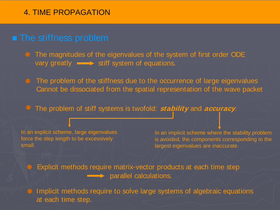
The magnitudes of the eigenvalues of the system of first order ODEvary greatly stiff system of equations.

The problem of stiff systems is twofold: stability and accuracy.

In an explicit scheme, large eigenvaluesforce the step length to be excessively small.

In an implicit scheme where the stability problemis avoided, the components corresponding to thelargest eigenvalues are inaccurate.

Explicit methods require matrix-vector products at each time stepparallel calculations.

Implicit methods require to solve large systems of algebraic equationsat each time step.

The stiffness problem

The problem of the stiffness due to the occurrence of large eigenvaluesCannot be dissociated from the spatial representation of the wave packet

4. TIME PROPAGATION

Fatunla’s method = explicit scheme for the solution of stiff systems of equations [7] :

' ( , ),f x=y y 1 2( , , , )my y y= …y

The solution ( )xy is approximated by the function ( )F x1 2( ) ( ) ( )x xF x I e I eΩ −Ω= − − − +a b c

( ) ( )1diag( , , )i i

i mω ωΩ = …

stiffness parameters

[7] J. Madronero and B. Piraux, Phys. Rev. A 80, 033409 (2009)

Fatunla’s method

4. TIME PROPAGATION

The stiffness parameters are the solution of a simple quadraticsystem of algebraic equations.

The stiffness parameters are related to the eigenfrequenciesof the atom + field system.

1 1( )n nx+ +≡y y nyis obtained from by a simple recurrence relationinvolving matrix-vector products only parallel calculations.

The local truncation error can be easily calculated allowing adaptative step sizes.

4. TIME PROPAGATION

2 21

1( ) ( ) 14

x y x xτ α= = +

First illustration

1(0) 1y =

2 (0) 12

y iα⎛ ⎞= −⎜ ⎟⎝ ⎠

Perturbed motion on a circular orbit in the complex plane of the point

=1( ) ( )y x y x=

which spirals slowly outward such that itsdistance from the origin x∀ is given by:

exact numτ τΔ = −

0.001α =0 40x π≤ ≤

Runge-Kutta

1 2y y′ =

2 1ixy y eα′ = − +

4. TIME PROPAGATION

The time propagation is performed in a basis of Coulomb Sturmian functions.photon energy: 0.057 a.u.peak intensity: 6 x 1014 Watt/cm2

pulse duration: 10 optical cycles 25 fs≈

Second illustration: ionisation of atomic hydrogen in its ground state by a strong low frequency pulsed field.

4. TIME PROPAGATION

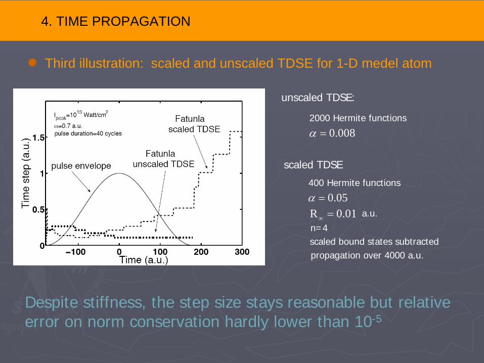
Third illustration: scaled and unscaled TDSE for 1-D medel atom

unscaled TDSE:

2000 Hermite functions

0.008α =

scaled TDSE

400 Hermite functions

0.05α =R 0.01∞ =n=4scaled bound states subtractedpropagation over 4000 a.u.

a.u.

Despite stiffness, the step size stays reasonable but relativeerror on norm conservation hardly lower than 10-5

4. TIME PROPAGATION

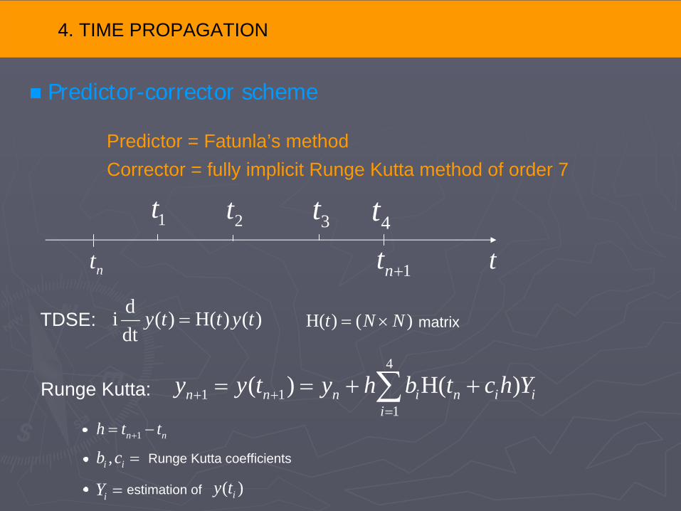
Predictor = Fatunla’s methodCorrector = fully implicit Runge Kutta method of order 7

nt t1nt +

1t 2t 3t 4t

TDSE:di ( ) H( ) ( )dt

y t t y t=

Runge Kutta: 4

1 11

( ) H( )n n n i n i ii

y y t y h b t c h Y+ +=

= = + +∑1n nh t t+= −

,i ib c = Runge Kutta coefficients

estimation ofiY = ( )iy t

matrixH( ) ( )t N N= ×

Predictor-corrector scheme

4. TIME PROPAGATION

iYThe are the solution of a system of dimension 4N :

1 11 1 14 4 1

4 41 1 44 4 4

H( ) H( )

H( ) H( )

n n n

n n n

Y y a t c h a t c h Yh

Y y a t c h a t c h Y

+ +⎛ ⎞ ⎛ ⎞ ⎛ ⎞⎛ ⎞⎜ ⎟ ⎜ ⎟ ⎜ ⎟⎜ ⎟= +⎜ ⎟ ⎜ ⎟ ⎜ ⎟⎜ ⎟⎜ ⎟ ⎜ ⎟ ⎜ ⎟⎜ ⎟+ +⎝ ⎠ ⎝ ⎠ ⎝ ⎠⎝ ⎠

In a predictor-corrector scheme, the vector in the RHS is is replaced by the result provided by the predictor no system to solve lack of accuracy.

Trick: Introduce a diagonal matrix D iterative procedure requiring to solve 4 systems of dimension N at each iterative step. The starting solution is provided by the predictor.

4. TIME PROPAGATION

( ) ( )1 11 1 1

( ) ( )4 44 4 4

( 1)11 11 1 14 4 1

( 1)41 1 44 44 4 4

H( ) 0

0 H( )

( )H( ) H( )

H( ) ( )H( )

j jn n

j jn n

jn n

jn n

Y d t c h Y yh

Y d t c h Y y

a d t c h a t c h Yh

a t c h a d t c h Y

−

−

⎛ ⎞ ⎛ ⎞+⎡ ⎤ ⎛ ⎞⎜ ⎟ ⎜ ⎟ ⎜ ⎟⎢ ⎥− =⎜ ⎟ ⎜ ⎟ ⎜ ⎟⎢ ⎥

⎜ ⎟⎜ ⎟ ⎜ ⎟⎢ ⎥+⎣ ⎦ ⎝ ⎠⎝ ⎠ ⎝ ⎠⎛ ⎞− + +⎡ ⎤⎜⎢ ⎥+ ⎜⎢ ⎥⎜⎢ ⎥+ − +⎣ ⎦ ⎝ ⎠

⎟⎟⎟

Each system is solved by means of biconjugate gradient algorithm which is an iterativeprocedure: maximum 2 iterations are needed!

The overal procedure only requires matrix-vector productsallowing parallel calculations.

5. OBSERVABLES

1( )2

ikxk x eϕ

π→∞ =

stationary phase theorem2

21( , )xi

txx t c et it

ψ ⎛ ⎞→∞ →∞ = ⎜ ⎟⎝ ⎠

2

2( , ) ( ) ( ) ( ) ( )n

ki tiE tn n k

nx t a t x e c k x e dkψ φ φ

+∞ −−

−∞= +∑ ∫

2( / 2)( , ) ( ) ( , )i mRRt R t e x tξϕ ξ ψ−=

/k x t=

( ) ,i kc k tR R

ϕ∞ ∞

⎛ ⎞= →∞⎜ ⎟

⎝ ⎠

Electron energy spectrum

The spectrum is ∝ tothe mod square of thescaled wave packet.

5. OBSERVABLES

Effect of an inaccurate description of a scaled bound state

5. OBSERVABLES

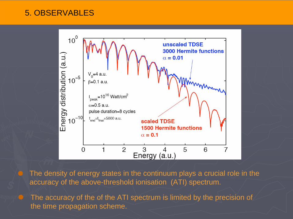
The density of energy states in the continuum plays a crucial role in the accuracy of the above-threshold ionisation (ATI) spectrum.

The accuracy of the of the ATI spectrum is limited by the precision ofthe time propagation scheme.

5. OBSERVABLES


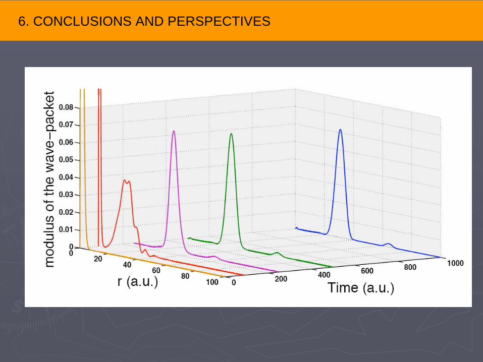
The time scaled coordinate approach is reflection free and allows to control the increasingly large phase gradients that develop during the time propagation.

Provided that the scaled bound states are extracted after the end ofthe pulse and when the harmonic potential has disappeared, Fatunla’smethod or the predictor-corrector scheme allows to propagate accuratelythe scaled wave packet to the genuine asymptotic region where the various channels are decoupled.

The electron energy spectra may be expressed in terms of the modulus square of the scaled wave packet.

Our investigations suggest that the optimal way to represent spatially the scaled wave packet is based on multi-resolution techniques.


Hamiltonian in hyperspherical coordinates.

Time dependent scaling of the hyperradius.

Use of the semi-classical boundary conditions in the double ionisation channels.

Solution of the TDSE associated to the interaction of helium with an external field:

new strategy for solving the time-dependent schrödinger...

Documents