new trends in geometric function theory...
TRANSCRIPT

International Journal of Mathematics and Mathematical Sciences
Guest Editors: Teodor Bulboaca , Nak Eun Cho, and Stanisława R. Kanas
New Trends in Geometric Function Theory 2011

New Trends in Geometric FunctionTheory 2011

International Journal of Mathematics andMathematical Sciences
New Trends in Geometric FunctionTheory 2011
Guest Editors: Teodor Bulboaca, Nak Eun Cho,and Stanisława R. Kanas

Copyright q 2012 Hindawi Publishing Corporation. All rights reserved.
This is a special issue published in “International Journal of Mathematics and Mathematical Sciences.” All articles are openaccess articles distributed under the Creative Commons Attribution License, which permits unrestricted use, distribution,and reproduction in any medium, provided the original work is properly cited.

Editorial BoardAsao Arai, JapanErik J. Balder, The NetherlandsA. Ballester-Bolinches, SpainMartino Bardi, ItalyP. Basarab-Horwath, SwedenPeter W. Bates, USAHeinrich Begehr, GermanyHoward E. Bell, CanadaKenneth S. Berenhaut, USAOscar Blasco, SpainMartin Bohner, USAHuseyin Bor, TurkeyTomasz Brzezinski, UKTeodor Bulboaca, RomaniaStefaan Caenepeel, BelgiumW. zu Castell, GermanyAlberto Cavicchioli, ItalyDer Chen Chang, USAShih Sen Chang, ChinaCharles E. Chidume, ItalyHi Jun Choe, Republic of KoreaColin Christopher, UKChristian Corda, ItalyRodica D. Costin, USAM.-E. Craioveanu, RomaniaRal E. Curto, USAPrabir Daripa, USAH. De Snoo, The NetherlandsLokenath Debnath, USAAndreas Defant, GermanyDavid E. Dobbs, USAS. S. Dragomir, AustraliaJewgeni Dshalalow, USAJ. Dydak, USAM. A. Efendiev, GermanyHans Engler, USARicardo Estrada, USAB. Forster-Heinlein, GermanyDalibor Froncek, USAXianguo Geng, China
Attila Gilanyi, HungaryJerome A. Goldstein, USASiegfried Gottwald, GermanyN. K. Govil, USAR. Grimshaw, UKHeinz Peter Gumm, GermanyS. M. Gusein-Zade, RussiaSeppo Hassi, FinlandPentti Haukkanen, FinlandJoseph Hilbe, USAHelge Holden, NorwayHenryk Hudzik, PolandPetru Jebelean, RomaniaPalle E. Jorgensen, USAShyam L. Kalla, KuwaitV. R. Khalilov, RussiaH. M. Kim, Republic of KoreaTaekyun Kim, Republic of KoreaEvgeny Korotyaev, GermanyAloys Krieg, GermanyWolfgang Kuhnel, GermanyIrena Lasiecka, USAYuri Latushkin, USABao Qin Li, USASongxiao Li, ChinaNoel G. Lloyd, UKR. Lowen, BelgiumAnil Maheshwari, CanadaRaul F. Manasevich, ChileB. N. Mandal, IndiaEnzo Luigi Mitidieri, ItalyVladimir Mityushev, PolandManfred Moller, South AfricaV. Nistor, USAEnrico Obrecht, ItalyChia-ven Pao, USAWen L. Pearn, TaiwanGelu Popescu, USAMihai Putinar, USAFeng Qi, China
Hernando Quevedo, MexicoJean Michel Rakotoson, FranceRobert H. Redfield, USAB. E. Rhoades, USAPaolo E. Ricci, ItalyFrederic Robert, FranceAlexander Rosa, CanadaAndrew Rosalsky, USAMisha Rudnev, UKStefan Samko, PortugalGideon Schechtman, IsraelNaseer Shahzad, Saudi ArabiaN. Shanmugalingam, USAZhongmin Shen, USAMarianna A. Shubov, USAH. S. Sidhu, AustraliaTheodore E. Simos, GreeceAndrzej Skowron, PolandFrank Sommen, BelgiumLinda R. Sons, USAF. C. R. Spieksma, BelgiumIlya M. Spitkovsky, USAMarco Squassina, ItalyH. M. Srivastava, CanadaYucai Su, ChinaPeter Takac, GermanyChun-Lei Tang, ChinaMichael M. Tom, USARam U. Verma, USAAndrei I. Volodin, CanadaLuc Vrancken, FranceDorothy I. Wallace, USAFrank Werner, GermanyRichard G. Wilson, MexicoIngo Witt, GermanyPei Yuan Wu, TaiwanSiamak Yassemi, IranA. Zayed, USAKaiming Zhao, CanadaYuxi Zheng, USA

Contents
New Trends in Geometric Function Theory 2011, Teodor Bulboaca, Nak Eun Cho,and Stanisława R. KanasVolume 2012, Article ID 976374, 2 pages
Toeplitz Operators with Essentially Radial Symbols, Roberto C. RaimondoVolume 2012, Article ID 492690, 14 pages
On Certain Subclasses of Analytic Functions Defined by Differential Subordination,Hesam MahzoonVolume 2011, Article ID 103521, 10 pages
On Certain Class of Analytic Functions Related to Cho-Kwon-Srivastava Operator,F. Ghanim and M. DarusVolume 2011, Article ID 459063, 11 pages
Stability of Admissible Functions, Rabha W. IbrahimVolume 2011, Article ID 342895, 7 pages
Domination Conditions for Families of Quasinearly Subharmonic Functions, Juhani RiihentausVolume 2011, Article ID 729849, 9 pages
On Starlike and Convex Functions with Respect to k-Symmetric Points,Afaf A. Ali Abubaker and Maslina DarusVolume 2011, Article ID 834064, 9 pages

Hindawi Publishing CorporationInternational Journal of Mathematics and Mathematical SciencesVolume 2012, Article ID 976374, 2 pagesdoi:10.1155/2012/976374
EditorialNew Trends in Geometric Function Theory 2011
Teodor Bulboaca,1 Nak Eun Cho,2 and Stanisława R. Kanas3
1 Faculty of Mathematics and Computer Science, Babes-Bolyai University, 400084 Cluj-Napoca, Romania2 Department of Applied Mathematics, Pukyong National University, Busan 608-737, Republic of Korea3 Department of Mathematics, Rzeszow University of Technology, 35-959 Rzeszow, Poland
Correspondence should be addressed to Teodor Bulboaca, [email protected]
Received 10 October 2011; Accepted 10 October 2011
Copyright q 2012 Teodor Bulboaca et al. This is an open access article distributed under theCreative Commons Attribution License, which permits unrestricted use, distribution, andreproduction in any medium, provided the original work is properly cited.
Geometric function theory is the branch of complex analysis which deals with the geometricproperties of analytic functions, founded around the turn of the 20th century. In spite of thefamous coefficient problem, the Bieberbach conjecture that was solved by Louis de Branges in1984 suggests various approaches and directions of studies in the geometric function theory.The cornerstone of geometric function theory is the theory of univalent functions, but newrelated topics appeared and developed with many interesting results and applications. Themajor andmost interesting topics are the theories of harmonic and quasiconformal mappings,and both are natural generalizations of the conformal mappings, but they were studiedseparately because of their natural significance and reciprocal differences.
The special issue has endeavored to publish research papers of the highest qualitywith appeal to the specialists in a field of geometric aspects of complex analysis and to broadmathematical community. We do hope that the distinctive aspects of the issue will bring thereader close to the subject of current research and leave the way open for a more direct andless ambivalent approach to the topics.
Inspired by the importance of geometric function theory and in order to stimulatefurther investigation in this area and the related topics, we decided to edit and publishthis second special issue (2011). Like in the previous one, we invited the authors to presenttheir original articles as well as review articles that will stimulate the continuing efforts indeveloping new results in geometric function theory. We believe that this second specialissue will improve our earlier mentioned goal, that is, to become an international forum forresearches to summarize the most recent developments and ideas in this field. The main aimof the special issue of our journal was to invite the authors to present their original articleswhich not only provide new results or methods but also may have a great impact on otherpeople in their efforts to broaden their knowledge and investigation.

2 International Journal of Mathematics and Mathematical Sciences
During the open period of this special issue, a number of 21 papers were submittedfor consideration of publication, but after the review process only 6 papers among thesesubmissions were accepted for publication.
We believe that the results established in the published paper will develop theunderstanding of the major new problems of this area and the related topics and will explorethe further applications in other fields of mathematics.
In “On starlike and convex functions with respect to k-symmetric points,” the authorsintroduced two subclasses of starlike and convex functions with respect to k-symmetricpoints, defined by using a new convolution operator. They determined inclusion propertiesbetween these classes, and the invariance of the classes with respect to the convolutionproduct with any arbitrary convex function with real coefficients was proved.
Starting from the fact that Y. Domar has given a condition that ensures the existenceof the largest subharmonic minorant of a given function and P. J. Rippon pointed outthat a modification of Domar’s argument gives a better result, in “Domination conditionsfor families of quasinearly subharmonic functions,” by using his previous, rather general andflexible modification of Domar’s original argument, the author extends their results both tothe subharmonic and quasinearly subharmonic settings.
Motivated by a multiplier transformation and some subclasses of meromorphic func-tions which have been defined by means of the Hadamard product of Cho-Kwon-Srivastavaoperator, the paper entitled “On certain class of analytic functions related to Cho-Kwon-Srivastavaoperator” deals with a similar transformation by means of the new Ghanim-Darus operator.Some inclusion properties, coefficient inequalities, sharp distortion inequalities, and theradius of starlikeness and convexity of a class related to this transformation are given.
The author of “Stability of admissible functions,”using the concept of the weaksubordination, examined the stability for a class of admissible functions in complex Banachspaces. The stability of analytic functions in the following classes is discussed: Bloch class,little Bloch class, hyperbolic little Bloch class, extend Bloch class, and Hilbert Hardy class.
The next paper “On certain subclasses of analytic functions defined by differentialsubordination” deals with some classes of analytic functions with negative coefficients, wherethe author introduces and studies certain subclasses of analytic functions which are definedby differential subordination. Coefficient inequalities, some properties of neighborhoods,distortion and covering theorems, radius of starlikeness, and convexity for these subclassesare presented.
Using the fact that for Toeplitz operators with radial symbols on the disk there areimportant results that characterize boundedness, compactness, and its relation to the Berezintransform, the author analyzed the relationship between the boundary behavior of theBerezin transform and the compactness of Tϕ, when ϕ ∈ L2(Ω) is essentially radial and Ωis a multiply-connected domain.
Acknowledgments
As editors of this special issue (2011), we would like to thank the authors for their valuablecontributions and also the reviewers of these papers for their major and fundamental work.The editors would like to thank the authors for their interesting contributions, the staff of thejournal for the unique opportunity that was offered, and the editorial office of the journal forthe support that has been provided during the preparation.
Teodor BulboacaNak Eun Cho
Stanisława R. Kanas

Hindawi Publishing CorporationInternational Journal of Mathematics and Mathematical SciencesVolume 2012, Article ID 492690, 14 pagesdoi:10.1155/2012/492690
Research ArticleToeplitz Operators with Essentially Radial Symbols
Roberto C. Raimondo1, 2
1 Division of Mathematics, Faculty of Statistical Sciences, University of Milano-Bicocca,Via Bicocca degli Arcimboldi 8, 20126 Milano, Italy
2 Department of Economics, University of Melbourne, Parkville, VIC 3010, Australia
Correspondence should be addressed to Roberto C. Raimondo, [email protected]
Received 1 July 2011; Revised 4 October 2011; Accepted 4 October 2011
Academic Editor: Nak Cho
Copyright q 2012 Roberto C. Raimondo. This is an open access article distributed under theCreative Commons Attribution License, which permits unrestricted use, distribution, andreproduction in any medium, provided the original work is properly cited.
For Topelitz operators with radial symbols on the disk, there are important results that characterizeboundedness, compactness, and its relation to the Berezin transform. The notion of essentiallyradial symbol is a natural extension, in the context of multiply-connected domains, of the notionof radial symbol on the disk. In this paper we analyze the relationship between the boundarybehavior of the Berezin transform and the compactness of Tφ when φ ∈ L2(Ω) is essentially radialand Ω is multiply-connected domains.
1. Introduction
Toeplitz operators are object of intense study. Many papers have been dedicated to the studyof these concrete class of operators generating many interesting results. A very importanttool to study the behavior of these operators is the Berezin transform. This tool is particularlyrelevant with its connections with quantum mechanics, especially in the case of the Toeplitzoperators on the Segal-Bargmann space. In this case, they arises naturally as anti-Wickquantization operators, and there is a natural equivalence between Toeplitz operators anda generalization of pseudodifferential operators, the so-called Weyl’s quantization.
In a fundamental paper, Axler and Zheng proved that, if S ∈ B(L2(D)) can be writtenas a finite sum of finite products of Toeplitz operators with L∞-symbols, then S is compactif and only if S has a Berezin transform which vanishes at the boundary of the disk D. Asthey expected, this result has been extended into several directions, and it has been provedeven for operators which are not of the Toeplitz type. Therefore it has been an important openproblem to characterize the class of operators for which the compactness is equivalent to thevanishing of the Berezin transform. Since there are operators which are not compact but havea Berezin transform which vanishes at the boundary, it is now clear that the two notions are
2 International Journal of Mathematics and Mathematical Sciences
not equivalent. Moreover, it is possible to show that in the context of Toeplitz operators thereare examples of unbounded symbols whose corresponding operators are bounded and evencompact.
Recently, many papers have been written in the case when the operator has an un-bounded radial symbol ϕ ∈ L2(D). Of course, for a square-integrable symbol, the Toeplitzoperator is densely defined but is not necessarily bounded. However, it is possible (see [1]of Grudsky and Vasilevski, [2] of Zorboska, and [3] of Korenblum and Zhu) to show thatoperators with unbounded radial symbols can have a very rich structure. Moreover, there isa very neat and elegant way to characterize boundedness and compactness. The reason beingthat the operators with radial symbols on the disk are diagonal operators. In this contextthe relation between compactness and the Berezin transform has been studied in depth, andinteresting results have been established.
In a previous paper (see [4]), the author showed that it is possible to extend thenotion of radial symbol when Ω is a bounded multiply-connected domain in the complexplane C, whose boundary ∂Ω consists of finitely many simple closed smooth analytic curvesγj (j = 1, 2, . . . , n) where γj are positively oriented with respect to Ω and γj ∩ γi = ∅ if i /= j.The key ingredient for this extension is to observe two facts. The first fact is that the structureof the Bergman kernel suggests that there is in any planar domain an internal region thatwe can neglect when we are interested in boundedness and compactness of the Toeplitzoperators with square integrable symbols. The second observation consists in exploiting thegeometry of the domain and conformal equivalence in order to partially recover the notion ofradial symbol. For this class of essentially radial symbols, the compactness and boundednesshave been studied and necessary and sufficient conditions established. In this paper wecarry forward our analysis by investigating the relationship between the compactness andthe vanishing of the Berezin transform. It is important to observe that in the case of thedisk the analysis uses the fact that the Berezin transform can be easily written in a simpleway since we can write explicitly an orthonormal basis, namely the collection of functions{√k + 1zk}∞k=0. In the case of a planar domain, this is not possible because it is very hard to
construct explicitly an orthonormal basis for the Bergman space. However, it is possible toreach interesting results that fully extend what it is known in the case of the disk.
The paper is organized as follows. In Section 2 we describe the setting where we work,give the relevant definitions, and state our main result. In Section 3 we prove the main resultand we study several important consequences.
2. Preliminaries
Let Ω be a bounded multiply-connected domain in the complex plane C, whose boundary∂Ω consists of finitely many simple closed smooth analytic curves γj (j = 1, 2, . . . , n)where γjare positively oriented with respect to Ω and γj ∩ γi = ∅ if i /= j. We also assume that γ1 is theboundary of the unbounded component of C\Ω. LetΩ1 be the bounded component of C\γ1,and Ωj (j = 2, . . . , n) the unbounded component of C \ γj , respectively, so that Ω =
⋂nj=1 Ωj .
For dν = (1/π)dx dy we consider the usual L2-space L2(Ω) = L2(Ω, dν). The Bergmanspace L2
a(Ω, dν), consisting of all holomorphic functions which are L2-integrable, is a closedsubspace of L2(Ω, dν)with the inner product given by
⟨f, g⟩=∫
Ωf(z)g(z)dν(z), (2.1)

International Journal of Mathematics and Mathematical Sciences 3
for f, g ∈ L2(Ω, dν). The Bergman projection is the orthogonal projection
P : L2(Ω, dν) −→ L2a(Ω, dν); (2.2)
it is well-known that for any f ∈ L2(Ω, dν)we have
Pf(w) =∫
Ωf(z)KΩ(z,w)dν(z), (2.3)
where KΩ is the Bergman reproducing kernel of Ω. For ϕ ∈ L∞(Ω, dν) the Toeplitz operatorTϕ : L2
a(Ω, dν) → L2a(Ω, dν) is defined by Tϕ = PMϕ whereMϕ is the standard multiplication
operator. A simple calculation shows that
Tϕf(z) =∫
Ωϕ(w)f(w)KΩ(w, z)dν(w). (2.4)
We use the symbol Δ to indicate the punctured disk {z ∈ C | 0 < |z| < 1}. Let Γ be any one ofthe domains Ω,Δ, Ωj (j = 2, . . . , n).
We call KΓ(z,w) the reproducing kernel of Γ, and we use the symbol kΓ(z,w) toindicate the normalized reproducing kernel; that is, kΓ(z, w) = KΓ(z,w)/KΓ(w,w)1/2.
For any A ∈ B(L2a(Γ, dν)), the space of bounded operators on L2
a(Γ, dν), we define A,the Berezin transform of A, by
A(w) =⟨AkΓw, k
Γw
⟩=∫
ΓAkΓw(z)k
Γw(z)dν(z), (2.5)
where kΓw(·) = KΓ(·, w)KΓ(w,w)−1/2.If ϕ ∈ L∞(Γ), then we indicate with the symbol ϕ the Berezin transform of the
associated Toeplitz operator Tϕ, and we have
ϕ(w) =∫
Γϕ(z)∣∣∣kΓw(z)
∣∣∣2dν(z). (2.6)
We remind the reader that it is well known that A ∈ C∞b(Γ) and we have ‖A‖∞ ≤ ‖A‖B(L2(Ω)).
It is possible, in the case of bounded symbols, to give a characterization of compactness usingthe Berezin transform (see [5, 6]).
We remind the reader that anyΩ bounded multiply-connected domain in the complexplane C, whose boundary ∂Ω consists of finitely many simple closed smooth analytic curvesγj (j = 1, 2, . . . , n), is conformally equivalent to a canonical bounded multiply-connecteddomain whose boundary consists of finitely many circles (see [7]). This means that it ispossible to find a conformally equivalent domain D =
⋂ni=1Di where D1 = {z ∈ C : |z| < 1}
andDj = {z ∈ C : |z−aj | > rj} for j = 2, . . . , n. Here aj ∈ D1 and 0 < rj < 1 with |aj−ak| > rj+rkif j /= k and 1 − |aj | > rj . Before we state the main result of this paper, we need to give a fewdefinitions.

4 International Journal of Mathematics and Mathematical Sciences
Definition 2.1. Let Ω =⋂ni=1 Ωi be a canonical bounded multiply-connected domain. One says
that the set of n + 1 functions P = {p0, p1, . . . , pn} is a ∂-partition for Ω if
(1) for every j = 0, 1, . . . , n, pj : Ω → [0, 1] is a Lipschitz, C∞-function;
(2) for every j = 2, . . . , n there exists an open set Wj ⊂ Ω and an εj > 0 such thatUεj = {ζ ∈ Ω : rj < |ζ − aj | < rj + εj} and the support of pj are contained inWj and
pj(ζ) = 1 ∀ζ ∈ Uεj ; (2.7)
(3) for j = 1 there exists an open set W1 ⊂ Ω and an ε1 > 0 such that Uε1 = {ζ ∈ Ω :1 − ε1 < |ζ| < 1} and the support of p1 are contained inW1 and
p1(ζ) = 1 ∀ζ ∈ Uε1 ; (2.8)
(4) for every j, k = 1, . . . , n, Wj ∩Wk = ∅, the set Ω \ (⋃nj=1Wj) is not empty and the
function
p0(ζ) = 1 ∀ζ ∈⎛
⎝n⋃
j=1
Wj
⎞
⎠
c
∩Ω,
p0(ζ) = 0 ∀ζ ∈ Uεk , k = 1, . . . , n,
(2.9)
(5) for any ζ ∈ Ω the following equation
n∑
k=0
pk(ζ) = 1 (2.10)
holds.
We also need the following.
Definition 2.2. A function ϕ : Ω =⋂ni=1 Ωi → C is said to be essentially radial if there exists
a conformally equivalent canonical bounded domain D =⋂ni=1Di such that, if the map Θ :
Ω → D is the conformal mapping from Ω onto D, then
(1) for every k = 2, . . . , n and for some εk > 0, one has
ϕ ◦Θ−1(z) = ϕ ◦Θ−1(|z − ak|) (2.11)
when z ∈ Uεk = {ζ ∈ Ω : rk < |ζ − ak| < rk + εk},(2) for k = 1 and for some ε1 > 0, one has
ϕ ◦Θ−1(z) = ϕ ◦Θ−1(|z|) (2.12)
when z ∈ Uε1 = {ζ ∈ Ω : 1 − ε1 < |ζ| < 1}.

International Journal of Mathematics and Mathematical Sciences 5
The reader should note that, in the case where it is necessary to stress the use of aspecific conformal equivalence, we will say that the map ϕ is essentially radial via Θ :⋂n=1 Ω → ⋂n
=1D . Moreover, we stress that in what follows, when we are working witha general multiply-connected domain and we have a conformal equivalence Θ :
⋂n=1 Ω →
⋂n=1D , we always assume that the ∂-partition is given on
⋂n=1D and transferred to
⋂n=1 Ω
through Θ in the natural way.
Definition 2.3. If ϕ ∈ L2(Ω) is an essentially radial function via Θ :⋂ni=1 Ωi → ⋂n
i=1Di, ϕj =ϕ · pj for any j = 1, . . . , n where P = {p0, p1, . . . , pn} is a ∂-partition for Ω then one defines then sequences
aϕ1 ={aϕ1(k)
}k∈Z+
, aϕ2 ={aϕ2(k)
}k∈Z+
, . . . , aϕn ={aϕn(k)
}k∈Z+
(2.13)
as follows: if j = 2, . . . , n,
aϕj (k) = rj
∫∞
rj
ϕj ◦Θ−1(rjs + aj)(k + 1)
r2k+1j
s2k+11s2ds ∀k ∈ Z+, (2.14)
and if j = 1,
aϕ1(k) =∫1
0ϕ1 ◦Θ−1(s)(k + 1)s2k+1ds ∀k ∈ Z+. (2.15)
At this point we can state the main result.
Theorem 2.4. Let ϕ ∈ L2(Ω) be an essentially radial function via Θ :⋂n=1 Ω → ⋂n
=1D andϕj = ϕ · pj for any j = 1, . . . , n where P = {p0, p1, . . . , pn} is a ∂-partition for Ω. If the operatorTϕ : L2
a(Ω, dν) → L2a(Ω, dν) is bounded and if for any j = 1, . . . , n the sequence aϕj = {aϕj (k)}k∈Z+
satisfies the following
supk∈Z+
{∣∣∣(k + 1)aϕj (k) − kaϕj (k − 1)
∣∣∣}<∞, (2.16)
then the operator Tϕ : L2a(Ω, dν) → L2
a(Ω, dν) is compact if and only if
limw→ ∂Ω
Tϕ(w) = 0. (2.17)
3. Canonical Multiply-Connected Domains andEssentially Radial Symbols
We concentrate on the relationship between compact Toeplitz operators and the Berezintransform. As we said in the introduction, Axler and Zheng have proved (see [5]) that ifD is the disk, S =
∑mi
∏mj
kTϕi,k , where ϕi,k ∈ L∞(D), then S is compact if and only if its
Berezin transform vanishes at the boundary of the disk. Their fundamental result has beenextended in several directions, in particular whenΩ is a general smoothly boundedmultiply-connected planar domain [6]. In this section we try to characterize the compactness in terms

6 International Journal of Mathematics and Mathematical Sciences
of the Berezin transform. In the next theorem, under a certain condition, we will show thatthe Berezin transform characterization of compactness still holds in this context.
In the case of the disk, it is possible to show that when the operator is radial then itsBerezin transform has a very special form. In fact, if ϕ : D → C is radial, then
Tϕ(z) =(1 − |z|2
)2∑(n + 1)
⟨Tϕen, en
⟩|z|2n, (3.1)
where, by definition,
en(z) =√n + 1zn ∀n ∈ Z+. (3.2)
Therefore to show that the vanishing of the Berezin transform implies compactness is equiv-alent, given that Tϕ is diagonal and to show that lim|z|→ 1(1 − |z|2)2∑(n + 1)〈Tϕen, en〉|z|2n = 0implies limn→∞〈Tϕen, en〉 = 0, Korenblum and Zhu realized this fact in their seminal paper[3], and, along this line, more was discovered by Zorboska (see [2]) and Grudsky andVasilevski (see [1]).
In the case of a multiply-connected domain, it is not possible to write things so neatly;however, we can exploit our estimates near the boundary to use similar arguments. In fact,for an essentially radial function, the values depend essentially on the distance from theboundary. Moreover, we can simplify our analysis if we use the fact that every multiply-connected domain is conformally equivalent to a canonical bounded multiply-connecteddomain whose boundary consists of finitely many circles. It is important to stress that in thecase of essentially radial symbol it is possible to exploit what has been done in the case of thedisk, but the operator is not a diagonal operator, and the Berezin transform is not particularlysimple to write in an explicit way.
In what follows the punctured disk Δ = {z ∈ C | 0 < |z| < 1} plays a very importantrole; for this reason we need the following.
Theorem 3.1. There exists an isomorphism I : L2(Δ) → L2(Ω1) such that
I(L2a(Δ))= L2
a(Ω1). (3.3)
Moreover, for any p ≥ 2 one has that Lpa(Δ) = Lpa(Ω1), and, for any (z,w) ∈ Δ2, the Bergman kernelsKΔ and KΩ1 satisfy the following equation:
KΔ(z,w) = KΩ1(z,w). (3.4)
Proof. Suppose that f ∈ L2a(Δ); this means that f is holomorphic on Δ, then we can write
down the Laurent expansion of f about 0, and we have
f(z) =∞∑
n=−∞anz
n. (3.5)

International Journal of Mathematics and Mathematical Sciences 7
This implies that |f(z)|2 =∑∞n,m=−∞anamz
nzm; therefore we have
∫
Δ
∣∣f(z)
∣∣2dν(z) =
∫
Δ
∞∑
n,m=−∞anamz
nzmdν(z)
=∫2π
0
∫1
0
∞∑
n,m=−∞anamr
n+m+1ei(n−m)θdr dθ
=∞∑
n,m=−∞anam
∫2π
0ei(n−m)θdθ
∫1
0rn+m+1dr
= 2π∞∑
n=−∞|an|2∫1
0r2n+1dr
= 2π
⎛
⎝∞∑
n/=−1|an|2[r2n+2
2n + 2
]1
0
+ |a−1|2∫1
0
1rdr
⎞
⎠.
(3.6)
The last equation, together with the fact that f is square-integrable, implies that an = 0 ifn ≤ −1. Then we can conclude that f has an holomorphic extension on Ω1. We define
I : L2(Δ) −→ L2(Ω1) (3.7)
in this way: if g ∈ L2(Δ), then Ig(z) = g(z) if z/= 0 and
Ig(0) =∫
Δg(z)dν(z). (3.8)
Then Ig ∈ L2(Ω1) and ‖Ig‖Ω1 = ‖g‖Δ. If f ∈ L2a(Δ), we have just shown that If ∈ L2
a(Ω1).Clearly I is injective and surjective, in fact if G ∈ L2(Ω1), then g = G|Δ is an element of L2(Δ)and I(g) = G. Then I is an isomorphism of L2(Δ) onto L2(Ω1) and I(L2
a(Δ)) = L2a(Ω1).
Moreover, observing that p > 2 implies ‖f‖Δ,2 ≤ ‖f‖Δ,p for any f ∈ Lp(Δ), we conclude thatLpa(Δ) = Lpa(Ω1).
Finally, it is easy to verify that for any f, g ∈ L2a(Δ) we have
⟨f, g⟩Δ =⟨If,Ig⟩Ω1
, (3.9)
and this fact implies, by the definition of the Bergman reproducing kernel, that
KΔ(z,w) = KΩ1(z,w), (3.10)
for any (z,w) ∈ Δ2.
In order to better explain our intuition, we remind the reader that we proved that, ifϕ ∈ L2(D) is an essentially radial function whereΩ is a bounded multiply-connected domainand if we define ϕj = ϕ · pj where j = 1, . . . , n where P = {p0, p1, . . . , pn} is a ∂-partitionfor Ω, then the fact that the operator Tϕ : L2
a(Ω, dν) → L2a(Ω, dν) is bounded (compact)

8 International Journal of Mathematics and Mathematical Sciences
is equivalent to fact, that for any j = 1, . . . , n, the operators Tϕj : L2a(Ωj , dν) → L2
a(Ωj , dν) arebounded (compact) (see [4]).
We start our investigation by focusing our attention on the case of bounded symbols.In fact, we prove the following.
Theorem 3.2. Let ϕ ∈ L∞(D) be an essentially radial function, if one defines ϕj = ϕ · pj where j =1, . . . , n and P is a ∂-partition for D. Then for the bounded operator Tϕ the following are equivalent:
(1) the operator Tϕ : L2a(D,dν) → L2
a(D,dν) is compact;
(2) for any j = 1, . . . , n one has
limk→∞
aϕj (k) = 0. (3.11)
Proof. Since ϕ ∈ L∞(D), we know that the operator Tϕ : L2a(Ω, dν) → L2
a(Ω, dν) is bounded,and we know that the boundedness (compactness) is equivalent to the fact that for any j =1, . . . , n the operators Tϕj : L
2(Dj, dν) → L2a(Dj, dν) are bounded (compact). If j = 2, . . . , n,
we observe that if we consider the following sets Δ0,1 = {z ∈ C : 0 < |z − a| < 1} and
Δaj ,rj = {z ∈ C : 0 < |z − aj | < rj} and the maps Δ0,1α→ Δaj ,rj
β→ Dj where α(z) = aj + rjzand β(w) = (w − aj)
−1r2j + aj and we use Proposition 1.1 in [8], we can claim that Tϕj =V −1β◦αTϕj◦β◦αVβ◦α where Vβ◦α : L2(Δ0,1) → L2(Dj) is an isomorphism of the Hilbert spaces.
Therefore Tϕj is compact if and only if Tϕj◦β◦α is compact. We also notice that the previoustheorem implies that function {
√k + 1zk} is an orthonormal basis for L2(Δ0,1), and this, in
turn, implies that the compactness of the operator Tϕj◦β◦α is equivalent to the fact that for thesequence aϕj = {aϕj (k)}k∈N
we have limk→∞aϕj (k) = 0 where, by definition,
aϕj (k) =∫
Δ0,1
ϕj ◦ β ◦ α(z)(k + 1)zkzkdz ∀m ∈ Z+. (3.12)
To complete the proof we observe that, since ϕj is radial and β ◦ α(r) = r−1rj + aj , then, aftera change of variable, we can rewrite the last integral, and hence the formula
aϕj (k) = rj
∫∞
rj
ϕj(rjs + aj
)(k + 1)
r2k+1j
s2k+11s2ds ∀m ∈ Z+ (3.13)
must hold for any j = 2, . . . , n. For the case j = 1 the proof is similar.
Now we can prove the following.
Theorem 3.3. Let ϕ ∈ L∞(Ω) be an essentially radial function via Θ :⋂n=1 Ω → ⋂n=1D , if one
defines ϕj = ϕ · pj where j = 1, . . . , n and P is a ∂-partition for Ω. Then for the bounded operator Tϕthe following are equivalent:
(1) the operator Tϕ : L2a(Ω, dν) → L2
a(Ω, dν) is compact;
(2) for any j = 1, . . . , n one has
limk→∞
aϕj (k) = 0. (3.14)

International Journal of Mathematics and Mathematical Sciences 9
Proof. We know that Ω is a regular domain, and therefore if Θ is a conformal mapping fromΩ onto D then the Bergman kernels of Ω and Θ(Ω) = D are related via KD(Θ(z),Θ(w))Θ′(z)Θ′(w) = KΩ(z,w) and the operator VΘf = Θ′ · f ◦ Θ is an isometry from L2(D) ontoL2(Ω) (see [8, Proposition 1.1]). In particular we have VΘP
D = PΩVΘ and this implies thatVΘTϕ = Tϕ◦Θ−1VΘ. Therefore the operator Tϕ is bounded if and only if for any j = 1, . . . , n theoperators Tϕj◦Θ−1 : L2
a(Dj, dν) → L2a(Dj, dν) are bounded (compact). Hence we can conclude
that the operator is bounded (compact) if for any j = 1, . . . , n we have
limk→∞
aϕj (k) = 0, (3.15)
where, by definition, if j = 2, . . . , n,
aϕj (k) = rj
∫∞
rj
ϕj ◦Θ−1(rjs + aj)(k + 1)
r2k+1j
s2k+11s2ds ∀k ∈ Z+, (3.16)
and if j = 1,
aϕ1(k) =∫1
0ϕ1 ◦Θ−1(s)(k + 1)s2k+1ds ∀k ∈ Z+. (3.17)
Theorem 3.4. Let ϕ ∈ L2(D) be an essentially radial function, if one defines ϕj = ϕ · pj wherej = 1, . . . , n and P is a ∂-partition for Ω and the operator Tϕ : L2
a(D,dν) → L2a(D,dν) is bounded
(compact) and if for any j = 1, . . . , n the sequences aϕj = {aϕj (k)}k∈Nare such that
supk∈N
{∣∣∣(k + 1)aϕj (k) − kaϕj (k − 1)
∣∣∣}
(3.18)
is finite, then the operator Tϕ : L2a(D,dν) → L2
a(D,dν) is compact if and only if
limw→ ∂D
Tϕ(w) = 0. (3.19)
Proof. We know that the operator under examination is bounded (compact) if and only if forany j = 1, . . . , n the operators
Tϕj : L2(Dj, dν
) −→ L2a
(Dj, dν
)(3.20)
are bounded (compact). If j = 2, . . . , n, we observe that if we consider the following setsΔ0,1 = {z ∈ C : 0 < |z − a| < 1} and Δaj ,rj = {z ∈ C : 0 < |z − aj | < rj} and the following maps
Δ0,1α−→ Δaj ,rj
β−→ Dj, (3.21)

10 International Journal of Mathematics and Mathematical Sciences
where α(z) = aj + rjz and β(w) = (w − aj)−1r2j + aj and we use Proposition 1.1 in [8], we canclaim that
Tϕj = V−1β◦αTϕj◦β◦αVβ◦α, (3.22)
where Vβ◦α : L2(Δ0,1) → L2(Dj) is an isomorphism of Hilbert’s spaces. Therefore Tϕjis compact if and only if Tϕj◦β◦α is compact. Since Tϕj◦β◦α : L2
a(Δ0,1) → L2a(Δ0,1) and
{√k + 1zk}∞k=0 is an orthonormal basis, a simple calculation shows that
aϕj (k) =⟨Tϕj◦β◦α
√k + 1zk,
√k + 1zk
⟩; (3.23)
therefore our assumption on aϕj = {aϕj (k)}k∈Nthat
supk∈Z+
{∣∣∣(k + 1)aϕj (k) − kaϕj (k − 1)
∣∣∣}<∞ (3.24)
implies (see [9, Theorem 6]) that the compactness of Tϕj◦β◦α is equivalent to the fact thatthe Berezin transform vanishes at the boundary. Since the case j = 1 is immediate, we canconclude, from what we proved so far, that for any j = 1, 2, . . . , n we have that compactnessis equivalent to the fact that limz→ ∂D ϕ
D (z) = 0. To complete the proof we set, for anyj = 1, . . . , n, Sj = {w ∈ Ω | pj(w) = 1} where {p1, . . . , pn} is in the ∂-partition for Ω. Bydefinition of ∂-partition, it follows that Sj ∩ Si = ∅ is j /= i, and we can write
ϕ(z) =⟨Tϕk
Dz , k
Dz
⟩
=∫
D
ϕ(w)∣∣∣kDz (w)
∣∣∣2dw
=∫
Sj
ϕ(w)∣∣∣kDz (w)
∣∣∣2dw +
∫
Ω∩Scj
ϕ(w)∣∣∣kDz (w)
∣∣∣2dw.
(3.25)
Since for any = 1, . . . , n the quantity∫
Sϕ(w)|kDz (w)|2dw can be written as
∫
S
⎛
⎜⎝ϕ(w)
(KDz
)2
∥∥∥K
Dz
∥∥∥2
2
⎞
⎟⎠
∥∥∥K
Dz
∥∥∥2
2∥∥KD
z
∥∥22
dw +∫
S
ϕ(w)
⎛
⎜⎝∣∣∣kDz (w)
∣∣∣2 −
(KDz
)2
∥∥KD
z
∥∥22
⎞
⎟⎠dw, (3.26)
we observe that the function θ(z,w) = (|kDz (w)|2 − (KDz )
2/‖KD
z ‖22) is bounded on the set S
and vanishes at the boundary.In fact, to prove this we remind the reader that there exists an isomorphism I :
L2(Δ0,1) → L2(Ω1) such that I(L2a(Δ0,1)) = L2
a(Ω1) and the Bergman kernels KΔ and KΩ1
satisfy the following equation KΔ(z,w) = KΩ1(z,w). If we define Δa,r = {z ∈ C : 0 <
|z − a| < r} and Oa,r = {z ∈ C : |z − a| > r}, then KOa,r (z,w) = r2/(r2 − (z − a) · (w − a))2

International Journal of Mathematics and Mathematical Sciences 11
for all (z,w) ∈ Oa,r × Oa,r . The well-known fact that the reproducing kernel of the unit diskis given by (1 − zw)−2 implies that KΔ0,1(z,w) = 1/(1 − z · w)2 for all (z,w) ∈ Δ0,1 × Δ0,1
therefore, by conformal mapping, that the reproducing kernel of Δa,r is KΔa,r (z,w) =r2/(r2 − (z − a) · (w − a))2 for all (z,w) ∈ Δa,r × Δa,r . If we define φ : Δa,r → Oa,r byφ(z) = (z − a)−1r2 + a and using the fact that KOa,r (φ(z), φ(w))φ′(z)φ′(w) = KΔa,r (z,w), weobtain thatKOa,r (z,w) = r2/(r2 − (z − a) · (w − a))2 for all (z,w) ∈ Oa,r ×Oa,r . SinceΩ1 = O0,1
and, for j = 2, . . . , n, Oaj ,rj = Ωj , then we prove that KDj (z,w) = r2j /(r2j − (z − aj) · (w − aj))2
if j = 2, . . . , n.Hence, for the function θ(z,w), we have
|θ(ζ, z)| =
∣∣∣∣∣∣∣
⎛
⎝
∑nm=0K
Dm(ζ, z)
∥∥KD
z
∥∥22
⎞
⎠
2
−
(KDz
)2
∥∥KD
z
∥∥22
∣∣∣∣∣∣∣
=
∣∣∣∣∣∣∣
(KDz
)2
∥∥KD
z
∥∥22
⎛
⎝1 +n∑
m/=
KDm(ζ, z)
KDz (ζ, z)
⎞
⎠
2
−
(KDz
)2
∥∥KD
z
∥∥22
∣∣∣∣∣∣∣
=
∣∣∣∣∣∣∣∣
(KDz
)2
∥∥KD
z
∥∥22
⎛
⎜⎝1 +
n∑
m/= m>0
r2m/(r2m − (z − am) · (ζ − am)
)2
r2/(r2 − (z − a) · (ζ − a)
)2 +KD
0 (ζ, z)
KDz (ζ, z)
⎞
⎟⎠
2
−
(KDz
)2
∥∥KD
z
∥∥22
∣∣∣∣∣∣∣∣
.
(3.27)
Hence it follows that θ(z,w) is bounded on the set S and goes to zero as it approachesthe boundary. Since ϕ ∈ L2(D) and D has a finite measure, we can conclude that, by thedominated convergence theorem, we have
limz→ ∂D
∫
S
ϕ(w)
⎛
⎜⎝∣∣∣kDz (w)
∣∣∣2 −
(KDz
)2
∥∥KD
z
∥∥22
⎞
⎟⎠dw = 0. (3.28)
Now we observe that Lemma 2 in [4] implies that
limz→ ∂D
∫
D∩S
⎛
⎜⎝ϕ(w)
⎛
⎜⎝
KDz∥
∥∥K
Dz
∥∥∥2
⎞
⎟⎠
2⎞
⎟⎠
⎛
⎜⎝
∥∥∥K
Dz
∥∥∥2∥
∥KDz
∥∥2
⎞
⎟⎠
2
dw (3.29)
goes to zero if and only limz→ ∂D ϕD (z) = 0, and a simple calculation shows that
∫
Ω∩Scj
ϕ(w)∣∣∣kDz (w)
∣∣∣2dw = 0. (3.30)

12 International Journal of Mathematics and Mathematical Sciences
Hence, as a consequence, we have shown that, if the conditions in the hypothesis hold, then
limz→ ∂D
ϕD(z) = 0, (3.31)
and this completes the proof since ∂D =⋃n
1 ∂D .
Now we can prove the following.
Theorem 3.5. Let ϕ ∈ L2(Ω) be an essentially radial function via Θ :⋂n=1 Ω → ⋂n
=1D andϕj = ϕ · pj for any j = 1, . . . , n where P = {p0, p1, . . . , pn} is a ∂-partition for Ω. If the operatorTϕ : L2
a(Ω, dν) → L2a(Ω, dν) is bounded and if for any j = 1, . . . , n the sequence aϕj = {aϕj (k)}k∈Z+
satisfies the following
supk∈Z+
{∣∣∣(k + 1)aϕj (k) − kaϕj (k − 1)
∣∣∣}<∞, (3.32)
then the operator Tϕ : L2a(Ω, dν) → L2
a(Ω, dν) is compact if and only if
limw→ ∂Ω
Tϕ(w) = 0. (3.33)
Proof. We know that Ω is a regular domain, and therefore, if Θ is a conformal mappingfrom Ω onto D then the Bergman kernels of Ω and Θ(Ω) = D are related viaKD(Θ(z),Θ(w))Θ′(z)Θ′(w) = KΩ(z,w) and the operator VΘf = Θ′ · f ◦ Θ is an isometryfrom L2(D) onto L2(Ω) (see [8, Proposition 1.1]). In particular we have VΘP
D = PΩVΘ andthis implies that VΘTϕ = Tϕ◦Θ−1VΘ. Therefore the operator Tϕ is bounded (compact) if andonly if the operator Tϕ◦Θ−1 : L2(D,dν) → L2
a(D,dν) is bounded (compact). In the previoustheorem we proved that the operator in exam is bounded (compact) if and only if for anyj = 1, . . . , n the operators Tϕj◦Θ−1 : L2
a(Dj, dν) → L2a(Dj, dν) are bounded (compact). Hence,
since the sequences aϕj = {aϕj (m)}m∈N
satisfy the stated properties, we can conclude that theoperators Tϕj◦Θ−1 : L2
a(Dj, dν) → L2a(Dj, dν) are compact if and only if for any j = 1, . . . , n we
have
limz→ ∂Dj
˜ϕj ◦Θ−1Dj
(z) = 0. (3.34)
Therefore it follows that
limz→ ∂D
ϕ ◦Θ−1D
(z) = 0, (3.35)
and, since Θ is a conformal mapping, this implies that
limz→ ∂Ω
ϕΩ(z) = 0. (3.36)

International Journal of Mathematics and Mathematical Sciences 13
Finally, we also observe that as a simple consequence we obtain the following.
Theorem 3.6. Let ϕ ∈ L2(Ω) be an essentially radial function via Θ :⋂n=1 Ω → ⋂n
=1D andϕj = ϕ · pj for any j = 1, . . . , n where P = {p0, p1, . . . , pn} is a ∂-partition for Ω. If the operatorTϕ : L2
a(Ω, dν) → L2a(Ω, dν) is bounded and if for any j = 1, . . . , n the sequence aϕj = {aϕj (k)}k∈Z+
satisfies the following
supk∈Z+
{∣∣∣k(aϕj (k) − aϕj (k − 1)
)∣∣∣}<∞, (3.37)
then the operator Tϕ : L2a(Ω, dν) → L2
a(Ω, dν) is compact if and only if
limw→ ∂Ω
Tϕ(w) = 0. (3.38)
Finally, we observe that it is also to recover as corollary the following.
Corollary 3.7. Let ϕ ∈ L2(Ω) be an essentially radial symbol via the conformal equivalenceΘ : Ω →D. If one defines ϕj = ϕ · pj where j = 1, . . . , n and P is a ∂-partition for Ω. Let us assume thatγφj = {γφj (m)}
m∈Nis in ∞(Z+) and that there is a constant C3 such that for j = 2, . . . , n
supτ∈[aj+rj ,∞)
∣∣∣∣∣ϕj ◦Θ(τ) − τ − aj
τ − rj − aj
∫ τ
aj+rjϕj ◦Θ
(y)(
rj(y − aj
)2
)
dy
∣∣∣∣∣< C3 (3.39)
and for j = 1
supτ∈[0,1]
∣∣∣∣∣ϕ1 ◦Θ(τ) − 1
1 − τ∫1
τ
ϕ1 ◦Θ(s)ds
∣∣∣∣∣< C3. (3.40)
Then the operator Tϕ : L2a(Ω, dν) → L2
a(Ω, dν) is compact if and only if
limw→ ∂Ω
Tϕ(w) = 0. (3.41)
The last corollary was also proved, in different way, in [4].
References
[1] S. Grudsky and N. Vasilevski, “Bergman-Toeplitz operators: radial component influence,” Integral Eq-uations and Operator Theory, vol. 40, no. 1, pp. 16–33, 2001.
[2] N. Zorboska, “The Berezin transform and radial operators,” Proceedings of the American MathematicalSociety, vol. 131, no. 3, pp. 793–800, 2003.
[3] B. Korenblum and K. H. Zhu, “An application of Tauberian theorems to Toeplitz operators,” Journal ofOperator Theory, vol. 33, no. 2, pp. 353–361, 1995.
[4] R. C. Raimondo, “Toeplitz operators on the bergman space of planar domains with essentially radialsymbols,” International Journal of Mathematics and Mathematical Sciences, vol. 2011, Article ID 164843, 26pages, 2011.

14 International Journal of Mathematics and Mathematical Sciences
[5] S. Axler and D. Zheng, “Compact operators via the Berezin transform,” Indiana University MathematicsJournal, vol. 47, no. 2, pp. 387–400, 1998.
[6] R. Raimondo, “Compact operators on the Bergman space of multiply-connected domains,” Proceedingsof the American Mathematical Society, vol. 129, no. 3, pp. 739–747, 2001.
[7] G. M. Goluzin, Geometric Theory of Functions of a Complex Variable, Translations of Mathematical Mono-graphs, Vol. 26, American Mathematical Society, Providence, RI, USA, 1969.
[8] J. Arazy, S. D. Fisher, and J. Peetre, “Hankel operators on planar domains,” Constructive Approximation,vol. 6, no. 2, pp. 113–138, 1990.
[9] Z. -H. Zhou,W. -L. Chen, and X. -T. Dong, “The Berezin transform and radial operators on the Bergmanspace of the unit ball,” Complex Analysis and Operator Theory. In press.

Hindawi Publishing CorporationInternational Journal of Mathematics and Mathematical SciencesVolume 2011, Article ID 103521, 10 pagesdoi:10.1155/2011/103521
Research ArticleOn Certain Subclasses of Analytic FunctionsDefined by Differential Subordination
Hesam Mahzoon
Department of Mathematics, Firoozkooh Branch, Islamic Azad University, Firoozkooh, Iran
Correspondence should be addressed to Hesam Mahzoon, mahzoon [email protected]
Received 3 June 2011; Accepted 25 August 2011
Academic Editor: Stanisława R. Kanas
Copyright q 2011 Hesam Mahzoon. This is an open access article distributed under the CreativeCommons Attribution License, which permits unrestricted use, distribution, and reproduction inany medium, provided the original work is properly cited.
We introduce and study certain subclasses of analytic functions which are defined by differentialsubordination. Coefficient inequalities, some properties of neighborhoods, distortion and coveringtheorems, radius of starlikeness, and convexity for these subclasses are given.
1. Introduction
Let T(j) be the class of analytic functions f of the form
f(z) = z −∞∑
k=j+1
akzk,
(ak ≥ 0, j ∈ N = {1, 2, . . .}), (1.1)
defined in the open unit disc U = {z ∈ C : |z| < 1}.
Let Ω be the class of functions ω analytic in U such that ω(0) = 0, |ω(z)| < 1.
For any two functions f and g in T(j), f is said to be subordinate to g that is denotedf ≺ g, if there exists an analytic function ω ∈ Ω such that f(z) = g(ω(z)) [1].
Definition 1.1 (see [2]). For n ∈ N and λ ≥ 0, the Al-Oboudi operator Dnλ: T(j) → T(j)
is defined as D0λf(z) = f(z), D1
λf(z) = (1 − λ)f(z) + λzf ′(z) = Dλf(z), and Dn
λf(z) =
Dλ(Dn−1λ f(z)).
For λ = 1, we get Salagean differential operator [3].

2 International Journal of Mathematics and Mathematical Sciences
Further, if f(z) = z −∑∞k=j+1 akz
k, then
Dnλf(z) = z −
∞∑
k=j+1
[1 + (k − 1)λ]nakzk (ak ≥ 0). (1.2)
For any function f ∈ T(j) and δ ≥ 0, the (j, δ)-neighborhood of f is defined as
Nj,δ
(f)=
⎧⎨
⎩g(z) = z −
∞∑
k=j+1
bkzk ∈ T(j) :
∞∑
k=j+1
k|ak − bk| ≤ δ⎫⎬
⎭. (1.3)
In particular, for the identity function e(z) = z, we see that
Nj,δ(e) =
⎧⎨
⎩g(z) = z −
∞∑
k=j+1
bkzk ∈ T(j) :
∞∑
k=j+1
k|bk| ≤ δ⎫⎬
⎭. (1.4)
The concept of neighborhoods was first introduced by Goodman [4] and then generalized byRuscheweyh [5].
Definition 1.2. A function f ∈ T(j) is said to be in the class Tj(n,m,A, B, λ) if
Dn+mλ f(z)Dnλf(z)
≺ 1 +Az1 + Bz
, z ∈ U, (1.5)
where n ∈ N0,m ∈ N, λ ≥ 1, and −1 ≤ B < A ≤ 1.
We observe that Tj(n,m, 1 − 2α,−1, 1) ≡ Tj(n,m, α) [6], Tj(0, 1, 1 − 2α,−1, 1) ≡S�j (α) [7], the class of starlike functions of order α and Tj(1, 1, 1 − 2α,−1, 1) ≡ Cj(α) [7], the
class of convex functions of order α.
2. Neighborhoods for the Class Tj(n,m,A, B, λ)
Theorem 2.1. A function f ∈ T(j) belongs to the class Tj(n,m,A, B, λ) if and only if
∞∑
k=j+1
[1 + (k − 1)λ]n{(1 − B)[1 + (k − 1)λ]m − (1 −A)
}ak ≤ A − B (2.1)
for n ∈ N0,m ∈ N, λ ≥ 1, and −1 ≤ B < A ≤ 1.
Proof. Let f ∈ Tj(n,m,A, B, λ). Then,
Dn+mλ
f(z)Dnλf(z)
≺ 1 +Az1 + Bz
, z ∈ U. (2.2)

International Journal of Mathematics and Mathematical Sciences 3
Therefore,
ω(z) =Dnλf(z) −Dn+m
λ f(z)BDn+m
λf(z) −ADn
λf(z)
. (2.3)
Hence,
|ω(z)| =
∣∣∣∣∣
Dnλf(z) −Dn+m
λ f(z)BDn+m
λ f(z) −ADnλf(z)
∣∣∣∣∣
=
∣∣∣∣∣
∑∞k=j+1 [1 + (k − 1)λ]n
{[1 + (k − 1)λ]m − 1
}akz
k
(A − B)z +∑∞k=j+1 [1 + (k − 1)λ]n
{B[1 + (k − 1)λ]m −A}akzk
∣∣∣∣∣< 1.
(2.4)
Thus,
R
{ ∑∞k=j+1 [1 + (k − 1)λ]n
{[1 + (k − 1)λ]m − 1
}akz
k
(A − B)z +∑∞k=j+1 [1 + (k − 1)λ]n
{B[1 + (k − 1)λ]m −A}akzk
}
< 1. (2.5)
Taking |z| = r, for sufficiently small r with 0 < r < 1, the denominator of (2.5) is positive andso it is positive for all r with 0 < r < 1, since ω(z) is analytic for |z| < 1. Then, inequality (2.5)yields
∞∑
k=j+1
[1 + (k − 1)λ]n{[1 + (k − 1)λ]m − 1
}akr
k
< (A − B)r + B∞∑
k=j+1
[1 + (k − 1)λ]n+makrk −A∞∑
k=j+1
[1 + (k − 1)λ]nakrk.
(2.6)
Equivalently,
∞∑
k=j+1
[1 + (k − 1)λ]n{(1 − B)[1 + (k − 1)λ]m − (1 −A)
}akr
k ≤ (A − B)r, (2.7)
and (2.1) follows upon letting r → 1.Conversely, for |z| = r, 0 < r < 1, we have rk < r. That is,
∞∑
k=j+1
[1 + (k − 1)λ]n{(1 − B)[1 + (k − 1)λ]m − (1 −A)
}akr
k
≤∞∑
k=j+1
[1 + (k − 1)λ]n{(1 − B)[1 + (k − 1)λ]m − (1 −A)
}akr ≤ (A − B)r.
(2.8)

4 International Journal of Mathematics and Mathematical Sciences
From (2.1), we have
∣∣∣∣∣∣
∞∑
k=j+1
[1 + (k − 1)λ]n{[1 + (k − 1)λ]m − 1
}akz
k
∣∣∣∣∣∣
≤∞∑
k=j+1
[1 + (k − 1)λ]n{[1 + (k − 1)λ]m − 1
}akr
k
< (A − B)r +∞∑
k=j+1
{B[1 + (k − 1)λ]m −A}[1 + (k − 1)λ]nakrk
<
∣∣∣∣∣∣(A − B)z +
∞∑
k=j+1
{B[1 + (k − 1)λ]m −A}[1 + (k − 1)λ]nakzk
∣∣∣∣∣∣.
(2.9)
This proves that
Dn+mλ
f(z)Dnλf(z)
≺ 1 +Az1 + Bz
, z ∈ U, (2.10)
and hence f ∈ Tj(n,m,A, B, λ).
Theorem 2.2. If
δ =(A − B)
(1 + λj
)n−1[(1 − B)(1 + λj)m − (1 −A)] , (2.11)
then Tj(n,m,A, B, λ) ⊂Nj,δ(e).
Proof. It follows from (2.1) that if f ∈ Tj(n,m,A, B, λ), then
(1 + λj
)n−1[(1 − B)(1 + λj)m − (1 −A)] ∞∑
k=j+1
kak ≤ (A − B), (2.12)
which implies
∞∑
k=j+1
kak ≤ (A − B)(1 + λj
)n−1[(1 − B)(1 + λj)m − (1 −A)] = δ. (2.13)
Using (1.4), we get the result.

International Journal of Mathematics and Mathematical Sciences 5
3. Neighborhoods for the Classes Rj(n,A, B, λ) and Pj(n,A, B, λ)
Definition 3.1. A function f ∈ T(j) is said to be in the class Rj(n,A, B, λ) if it satisfies
(Dnλf(z)
)′ ≺ 1 +Az1 + Bz
(z ∈ U), (3.1)
where −1 ≤ B < A ≤ 1, λ ≥ 1 and n ∈ N0.
Definition 3.2. A function f ∈ T(j) is said to be in the class Pj(n,A, B, λ) if it satisfies
Dnλf(z)z
≺ 1 +Az1 + Bz
(z ∈ U), (3.2)
where −1 ≤ B < A ≤ 1, λ ≥ 1 and n ∈ N0.
Lemma 3.3. A function f ∈ T(j) belongs to the class Rj(n,A, B, λ) if and only if
∞∑
k=j+1
(1 − B)[1 + (k − 1)λ]n+1ak ≤ A − B. (3.3)
Lemma 3.4. A function f ∈ T(j) belongs to the class Pj(n,A, B, λ) if and only if
∞∑
k=j+1
(1 − B)[1 + (k − 1)λ]nak ≤ A − B. (3.4)
Theorem 3.5. Rj(n,A, B, λ) ⊂ Nj,δ(e), where
δ =(A − B)
[1 + λj
]n(1 − B) . (3.5)
Proof. If f ∈ Rj(n,A, B, λ), we have
[1 + λj
]n∞∑
k=j+1
(1 − B)kak ≤ A − B, (3.6)
which implies∞∑
k=j+1
kak ≤ (A − B)[1 + λj
]n(1 − B) = δ. (3.7)
Theorem 3.6. Pj(n,A, B, λ) ⊂ Nj,δ(e), where
δ =(A − B)
[1 + λj
]n−1(1 − B). (3.8)

6 International Journal of Mathematics and Mathematical Sciences
Proof. If f ∈ Pj(n,A, B, λ), we have
[1 + λj
]n−1 ∞∑
k=j+1
(1 − B)kak ≤ A − B, (3.9)
which implies
∞∑
k=j+1
kak ≤ (A − B)[1 + λj
]n−1(1 − B)= δ. (3.10)
Thus, in view of condition (1.4), we get the required result of Theorem 3.6.
4. Neighborhood of the Class Kλj (n,m,A, B,C,D)
Definition 4.1. A function f ∈ T(j) is said to be in the class Kλj (n,m,A, B,C,D) if it satisfies
∣∣∣∣f(z)g(z)
− 1∣∣∣∣ <
A − B1 − B , z ∈ U, (4.1)
for −1 ≤ B < A ≤ 1, −1 ≤ D < C ≤ 1, λ ≥ 1 and g ∈ Tj(n,m,C,D, λ).
Theorem 4.2. For g ∈ Tj(n,m,C,D, λ), one has Nj,δ(g) ⊂ Kλj (n,m,A, B,C,D) and
1 −A1 − B = 1 −
[1 + λj
]n−1[(1 −D)[1 + λj
]m − (1 − C)]δ[1 + λj
]n[(1 −D)[1 + λj
]m − (1 − C)] − (C −D), (4.2)
where
δ ≤ (1 −D)(1 + λj
) − (C −D)[1 + λj
]1−n{(1 −D)[1 + λj
]m − (1 − C)}−1. (4.3)
Proof. Let f ∈ Nj,δ(g) for g ∈ Tj(n,m,C,D, λ). Then,
∞∑
k=j+1
k|ak − bk| ≤ δ,∞∑
k=j+1
bk ≤ C −D[1 + λj
]n[(1 −D)[1 + λj
]m − (1 − C)] . (4.4)

International Journal of Mathematics and Mathematical Sciences 7
Consider∣∣∣∣f(z)g(z)
− 1∣∣∣∣ ≤∑∞
k=j+1|ak − bk|1 −∑∞
k=j+1 bk
≤ δ(1 + λj
)
[1 + λj
]n{(1 −D)[1 + λj
]m − (1 − C)}[1 + λj
]n{(1 −D)[1 + λj
]m − (1 − C)} − (C −D)
=
[1 + λj
]n−1{(1 −D)[1 + λj
]m − (1 − C)}δ[1 + λj
]n{(1 −D)[1 + λj
]m − (1 − C)} − (C −D)
=A − B1 − B .
(4.5)
This implies that f ∈ Kλj (n,m,A, B,C,D).
5. Distortion and Covering Theorems
Theorem 5.1. If f ∈ Tj(n,m,A, B, λ), then
r − A − B(1 + jλ
)n{(1 − B)(1 + jλ)m − (1 −A)}rj+1
≤ ∣∣f(z)∣∣ ≤ r + A − B(1 + jλ
)n{(1 − B)(1 + jλ)m − (1 −A)}rj+1 (0 < |z| = r < 1),
(5.1)
with equality for
f(z) = z − A − B(1 + jλ
)n{(1 − B)(1 + jλ)m − (1 −A)}rj+1 (z = ±r). (5.2)
Proof. In view of Theorem 2.1, we have
(1 + jλ
)n{(1 − B)(1 + jλ)m − (1 −A)} ∞∑
k=j+1
ak
≤∞∑
k=j+1
[1 + (k − 1)λ]n{(1 − B)[1 + (k − 1)λ]m − (1 −A)
}ak ≤ A − B.
(5.3)
Hence,
∣∣f(z)
∣∣ ≤ r +
∞∑
k=j+1
akrk ≤ r + rj+1
∞∑
k=j+1
ak ≤ r + A − B(1 + jλ
)n{(1 − B)(1 + jλ)m − (1 −A)}rj+1,
∣∣f(z)
∣∣ ≥ r −
∞∑
k=j+1
akrk ≥ r − rj+1
∞∑
k=j+1
ak ≥ r − A − B(1 + jλ
)n{(1 − B)(1 + jλ)m − (1 −A)}rj+1.
(5.4)
This completes the proof.

8 International Journal of Mathematics and Mathematical Sciences
Theorem 5.2. Any function f ∈ Tj(n,m,A, B, λ) maps the disk |z| < 1 onto a domain that containsthe disk
|w| < 1 − A − B(1 + jλ
)n{(1 − B)(1 + jλ)m − (1 −A)} . (5.5)
Proof. The proof follows upon letting r → 1 in Theorem 5.1.
Theorem 5.3. If f ∈ Tj(n,m,A, B, λ), then
1 − (A − B)(1 + jλ
)n−1{(1 − B)(1 + jλ)m − (1 −A)}r
j
≤ ∣∣f ′(z)∣∣ ≤ 1 +
A − B(1 + jλ
)n−1{(1 − B)(1 + jλ)m − (1 −A)}r
j (0 < |z| = r < 1),
(5.6)
with equality for
f(z) = z − A − B(1 + jλ
)n−1{(1 − B)(1 + jλ)m − (1 −A)}z
j+1 (z = ±r). (5.7)
Proof. We have
∣∣f ′(z)
∣∣ ≤ 1 +
∞∑
k=j+1
kak|z|k−1 ≤ 1 + rj∞∑
k=j+1
kak. (5.8)
In view of Theorem 2.1,
∞∑
k=j+1
kak ≤ A − B(1 + jλ
)n−1{(1 − B)(1 + jλ)m − (1 −A)} . (5.9)
Thus,
∣∣f ′(z)
∣∣ ≤ 1 +
A − B(1 + jλ
)n−1{(1 − B)(1 + jλ)m − (1 −A)}r
j . (5.10)
On the other hand,
∣∣f ′(z)
∣∣ ≥ 1 −
∞∑
k=j+1
kak|z|k−1 ≥ 1 − rj∞∑
k=j+1
kak
≥ 1 − A − B(1 + jλ
)n−1{(1 − B)(1 + jλ)m − (1 −A)}r
j .
(5.11)
This completes the proof.

International Journal of Mathematics and Mathematical Sciences 9
6. Radii of Starlikeness and Convexity
In this section, we find the radius of starlikeness of order ρ and the radius of convexity oforder ρ for functions in the class Tj(n,m,A, B, λ).
Theorem 6.1. If f ∈ Tj(n,m,A, B, λ), then f is starlike of order ρ, (0 ≤ ρ < 1) in |z| <r1(n,m,A, B, λ, ρ), where
r1(n,m,A, B, λ, ρ
)= infk
[[1 + (k − 1)λ]n
{(1 − B)[1 + (k − 1)λ]m − (1 −A)
}(1 − ρ)
(k − ρ)(A − B)
]1/(k−1).
(6.1)
Proof. It is sufficient to show that |z(f ′(z)/f(z)) − 1| ≤ 1 − ρ (0 ≤ ρ < 1) for |z| <r1(n,m,A, B, λ, ρ).
We have
∣∣∣∣zf ′(z)f(z)
− 1∣∣∣∣ ≤∑∞
k=j+1(k − 1)ak|z|k−1
1 −∑∞k=j+1 ak|z|k−1
. (6.2)
Thus, |z(f ′(z)/f(z)) − 1| ≤ 1 − ρ if
∞∑
k=j+1
(k − ρ)ak|z|k−1(1 − ρ) ≤ 1. (6.3)
Hence, by Theorem 2.1, (6.3)will be true if
(k − ρ)|z|k−1(1 − ρ) ≤ [1 + (k − 1)λ]n
{(1 − B)[1 + (k − 1)λ]m − (1 −A)
}
(A − B) (6.4)
or if
|z| ≤[[1 + (k − 1)λ]n
{(1 − B)[1 + (k − 1)λ]m − (1 −A)
}(1 − ρ)
(k − ρ)(A − B)
]1/(k−1)(k ≥ j + 1
). (6.5)
This completes the proof.
Theorem 6.2. If f ∈ Tj(n,m,A, B, λ), then f is convex of order ρ, (0 ≤ ρ < 1) in |z| <r2(n,m,A, B, λ, ρ), where
r2(n,m,A, B, λ, ρ
)= inf
k
[[1 + (k − 1)λ]n
{(1 − B)[1 + (k − 1)λ]m − (1 −A)
}(1 − ρ)
(k − ρ)(A − B)
]1/(k−1).
(6.6)

10 International Journal of Mathematics and Mathematical Sciences
Proof. It is sufficient to show that |z(f ′′(z)/f ′(z))| ≤ 1 − ρ (0 ≤ ρ < 1) for |z| <r1(n,m,A, B, λ, ρ).
We have
∣∣∣∣zf ′′(z)f ′(z)
∣∣∣∣ ≤∑∞
k=j+1 k(k − 1)ak|z|k−1
1 −∑∞k=j+1 kak|z|k−1
. (6.7)
Thus, |z(f ′′(z)/f ′(z))| ≤ 1 − ρ if
∞∑
k=j+1
k(k − ρ)ak|z|k−1(1 − ρ) ≤ 1. (6.8)
Hence, by Theorem 2.1, (6.8)will be true if
k(k − ρ)|z|k−1(1 − ρ) ≤ [1 + (k − 1)λ]n
{(1 − B)[1 + (k − 1)λ]m − (1 −A)
}
(A − B) (6.9)
or if
|z| ≤[[1 + (k − 1)λ]n
{(1 − B)[1 + (k − 1)λ]m − (1 −A)
}(1 − ρ)
k(k − ρ)(A − B)
]1/(k−1)(k ≥ j + 1
). (6.10)
This completes the proof.
Acknowledgment
The author wish to thank the referee for his valuable suggestions.
References
[1] P. L. Duren, Univalent Functions, Springer, New York, NY, USA, 1983.[2] F. M. Al-Oboudi, “On univalent functions defined by a generalized Salagean operator,” International
Journal of Mathematics and Mathematical Sciences, no. 25–28, pp. 1429–1436, 2004.[3] G. Salagean, “Subclasses of univalent functions,” in Complex analysis—Fifth Romanian-Finnish Seminar,
Part 1 (Bucharest, 1981), vol. 1013 of Lecture Notes in Math., pp. 362–372, Springer, Berlin, Germany, 1983.[4] A. W. Goodman, “Univalent functions and nonanalytic curves,” Proceedings of the American
Mathematical Society, vol. 8, pp. 598–601, 1957.[5] S. Ruscheweyh, “Neighborhoods of univalent functions,” Proceedings of the American Mathematical
Society, vol. 81, no. 4, pp. 521–527, 1981.[6] M. K. Aouf, “Neighborhoods of certain classes of analytic functions with negative coefficients,”
International Journal of Mathematics and Mathematical Sciences, vol. 2006, Article ID 38258, 6 pages, 2006.[7] M. I. S. Robertson, “On the theory of univalent functions,” Annals of Mathematics. Second Series, vol. 37,
no. 2, pp. 374–408, 1936.

Hindawi Publishing CorporationInternational Journal of Mathematics and Mathematical SciencesVolume 2011, Article ID 459063, 11 pagesdoi:10.1155/2011/459063
Research ArticleOn Certain Class of Analytic Functions Related toCho-Kwon-Srivastava Operator
F. Ghanim1 and M. Darus2
1 Faculty of Management, Multimedia University, Selangor D. Ehsan, 63100 Cyberjaya, Malaysia2 School of Mathematical Sciences, Faculty of Science and Technology, Universiti Kebangsaan Malaysia,Selangor D. Ehsan, 43600 Bangi, Malaysia
Correspondence should be addressed to M. Darus, [email protected]
Received 27 March 2011; Accepted 29 August 2011
Academic Editor: Stanisława R. Kanas
Copyright q 2011 F. Ghanim and M. Darus. This is an open access article distributed underthe Creative Commons Attribution License, which permits unrestricted use, distribution, andreproduction in any medium, provided the original work is properly cited.
Motivated by a multiplier transformation and some subclasses of meromorphic functions whichwere defined by means of the Hadamard product of the Cho-Kwon-Srivastava operator, we definehere a similar transformation by means of the Ghanim and Darus operator. A class related to thistransformation will be introduced and the properties will be discussed.
1. Introduction
Let Σ denote the class of meromorphic functions f(z) normalized by
f(z) =1z+
∞∑
n=1
anzn, (1.1)
which are analytic in the punctured unit disk U = {z : 0 < |z| < 1}. For 0 ≤ β, we denoteby S∗(β) and k(β) the subclasses of Σ consisting of all meromorphic functions which are,respectively, starlike of order β and convex of order β inU (cf. e.g., [1–4]).
For functions fj(z) (j = 1; 2) defined by
fj(z) =1z+
∞∑
n=1
an,jzn, (1.2)

2 International Journal of Mathematics and Mathematical Sciences
we denote the Hadamard product (or convolution) of f1(z) and f2(z) by
(f1 ∗ f2
)=
1z+
∞∑
n=1
an,1an,2zn. (1.3)
Let us define the function φ(α, β; z) by
φ(α, β; z
)=
1z+
∞∑
n=0
∣∣∣∣∣
(α)n+1(β)n+1
∣∣∣∣∣zn, (1.4)
for β /= 0,−1,−2, . . ., and α ∈ C/{0}, where (λ)n = λ(λ + 1)n+1 is the Pochhammer symbol. Wenote that
φ(α, β; z
)=
1z
2F1(1, α, β; z
), (1.5)
where
2F1(b, α, β; z
)=
∞∑
n=0
(b)n(α)n(β)n
zn
n!(1.6)
is the well-known Gaussian hypergeometric function.Let us put
qλ,μ(z) =1z+
∞∑
n=1
(λ
n + 1 + λ
)μ
zn, λ > 0, μ ≥ 0. (1.7)
Corresponding to the functions φ(α, β; z) and qλ,μ(z) and using the Hadamard product forf(z) ∈ Σ, we define a new linear operator L(α, β, λ, μ)f(z) on
∑by
L(α, β, λ, μ
)f(z) =
(f(z) ∗ φ(α, β; z) ∗ qλ,μ(z)
)
=1z+
∞∑
n=1
∣∣∣∣∣
(α)n+1(β)n+1
∣∣∣∣∣
(λ
n + 1 + λ
)μ
anzn.
(1.8)
The meromorphic functions with the generalized hypergeometric functions were consideredrecently by Dziok and Srivastava [5, 6], Liu [7], Liu and Srivastava [8–10], and Cho and Kim[11].
For a function f ∈ L(α, β, λ, μ)f(z), we define
Iμ,0α,β,λ
= L(α, β, λ, μ
)f(z), (1.9)

International Journal of Mathematics and Mathematical Sciences 3
and, for k = 1, 2, 3, . . .,
Iμ,k
α,β,λf(z) = z
(Ik−1L
(α, β, λ, μ
)f(z)
)′+2z
=1z+
∞∑
n=1
nk∣∣∣∣∣
(α)n+1(β)n+1
∣∣∣∣∣
(λ
n + 1 + λ
)μ
anzn.
(1.10)
Note that if n = β, k = 0, the operator Iμ,0α,n,λ
reduced to the one introduced by Cho et al. [12]
for μ ∈ N0 = N ∪ 0. It was known that the definition of the operator Iμ,0α,n,λ was motivatedessentially by the Choi-Saigo-Srivastava operator [13] for analytic functions, which includesa simpler integral operator studied earlier by Noor [14] and others (cf. [15–17]). Note alsothe operator I0,kα,β has been recently introduced and studied by Ghanim and Darus [18] andGhanim et al. [19], respectively. To our best knowledge, the recent work regarding operatorIμ,0α,n,λ was charmingly studied by Piejko and Sokol [20]. Moreover, the operator Iμ,kα,β,λ was thendefined and studied by Ghanim and Darus [21]. In the same direction, we will study for theoperator Iμ,k
α,β,λgiven in (1.10).
Now, it follows from (1.8) and (1.10) that
z(Iμ,k
α,β,λf(z))′
= αIμ,kα+1,β,λf(z) − (α + 1)Iμ,kα,β,λf(z). (1.11)
Making use of the operator Iμ,kα,β,λf(z), we say that a function f(z) ∈ Σ is in the classΣμ,k
α,β,λ(A,B)if it satisfies the following subordination condition:
z(Iμ,k
α,β,λf(z)
)′
Iμ,k
α,β,λf(z)
≺ 1 − (B −A)w(z)1 + Bw(z)
, z ∈ U; −1 ≤ B < A ≤ 1. (1.12)
Furthermore, we say that a function f(z) ∈ Σμ,k,+α,β,λ(A,B) is a subclass of the class Σμ,k
α,β,λ(A,B)of the form
f(z) =1z+
∞∑
n=1
anzn (an > 0, z ∈ U). (1.13)
The main object of this paper is to present several inclusion relations and other properties offunctions in the classes Σμ,k
α,β,λ(A,B) and Σμ,k,+α,β,λ(A,B) which we have introduced here.
2. Main Results
We begin by recalling the following result (popularly known as Jack’s Lemma), which wewill apply in proving our first inclusion theorem.

4 International Journal of Mathematics and Mathematical Sciences
Lemma 2.1 (see [Jack’s Lemma] [22]). Let the (nonconstant) functionw(z) be analytic inU withw(0) = 0. If |w(z)| attains its maximum value on the circle |z| = r < 1 at a point z0 ∈ U, then
z0w′(z0) = γw(z0), (2.1)
where γ is a real number and γ ≥ 1.
Theorem 2.2. If
α >(A − B)1 + B
(−1 < B < A ≤ 1), (2.2)
then
Σμ,k
α+1,β,λ(A,B) ⊂ Σμ,k
α,β,λ(A,B). (2.3)
Proof. Let f ∈ Σμ,k
α+1, β,λ(A,B), and suppose that
z(Iμ,k
α,β,λf(z))′
Iμ,k
α,β,λf(z)= 1 − (B −A)w(z)
1 + Bw(z), (2.4)
where the functionw(z) is either analytic or meromorphic inU, withw(0) = 0. By using (2.4)and (1.11), we have
αIμ,k
α+1,β,λf(z)
Iμ,k
α,β,λf(z)=α + [αB − (A − B)]w(z)
1 + Bw(z). (2.5)
Upon differentiating both sides of (2.5) with respect to z logarithmically and using theidentity (1.11), we obtain
z(Iμ,k
α+1,β,λf(z))′
Iμ,k
α,β,λf(z)
= 1 − (B −A)w(z)1 + Bw(z)
− (A − B)zw′(z)[1 + Bw(z)](α + [αB − (A − B)]w(z))
. (2.6)
We suppose now that
max|z|≤|z0|
|w(z)| = |w(z0)| = 1 (z ∈ U) (2.7)
and apply Jack’s Lemma, we thus find that
z0w′(z0) = γw(z0)
(γ ≥ 1
). (2.8)

International Journal of Mathematics and Mathematical Sciences 5
By writing
w(z0) = eiθ (0 ≤ θ < 2π) (2.9)
and setting z = z0 in (2.6), we find after some computations that
∣∣∣∣∣∣∣
z0(Iμ,k
α+1,β,λf(z0))′
+ Iμ,kα+1,β,λf(z0)
Bz0(Iμ,k
α+1,β,λf(z0))′
+AIμ,kα+1,β,λf(z0)
∣∣∣∣∣∣∣
2
− 1 =
∣∣∣∣∣
(α + γ
)+ [αB − (A − B)]eiθ
α +[αB − γ − (A − B)]eiθ
∣∣∣∣∣
2
− 1
=2γ(1 + cos θ)[α(B + 1) − (A − B)]
∣∣α +
[αB − γ − (A − B)]eiθ∣∣2
.
(2.10)
Set
g(θ) = 2γ(1 + cos θ)[α(B + 1) − (A − B)]. (2.11)
Then, by hypothesis, we have
g(0) = 4γ[α(B + 1) − (A − B)] ≥ 0,
g(π) = 0,(2.12)
which, together, imply that
g(θ) ≥ 0 (0 ≤ θ < 2π). (2.13)
View of (2.13) and (2.10) would obviously contradict our hypothesis that
f ∈ Σμ,k
α+1,β,λ(A,B). (2.14)
Hence, we must have
|w(z)| < 1 (z ∈ U), (2.15)
and we conclude from (2.4) that
f ∈ Σμ,k
α,β,λ(A,B). (2.16)
The proof of Theorem 2.2 is thus complete.

6 International Journal of Mathematics and Mathematical Sciences
3. Properties of the Class f ∈ Σμ,k,+α,β,λ(A,B)
Throughout this section, we assume further that α, β > 0 and
A + B ≤ 0 (−1 < B < A ≤ 1). (3.1)
We first determine a necessary and sufficient condition for a function f ∈ Σ of the form(1.13) to be in the class f ∈ Σμ,k, +
α,β,λ (A,B) of meromorphically univalent functions with positivecoefficients.
Theorem 3.1. Let f ∈ Σ be given by (1.13). Then f ∈ Σμ,k,+α,β,λ(A,B) if and only if
∞∑
n=1
nk[n(1 − B) + (1 −A)]|(α)n+1|∣∣(β)n+1
∣∣
(λ
n + 1 + λ
)μ
|an| ≤ A − B, (3.2)
where, for convenience, the result is sharp for the function f(z) given by
f(z) =1z+
(A − B)(n + 1 + λ)μ∣∣(β)n+1
∣∣
nkλμ[n(1 − B) + (1 −A)]|(α)n+1|zn, (3.3)
for all z/= 0.
Proof. Suppose that the function f ∈ Σ is given by (1.13) and is in the class Σμ,k,+α,β,λ
(A,B). Then,from (1.13) and (1.12), we find that
∣∣∣∣∣∣∣
z(Iμ,k
α,β,λf(z))′
+ Iμ,kα,β,λf(z)
Bz(Iμ,k
α,β,λf(z))′
+AIμ,kα,β,λf(z)
∣∣∣∣∣∣∣
=
∣∣∣∣∣
∑∞n=1 n
k(n + 1)(|(α)n+1|/
∣∣(β)n+1
∣∣)(λ/(n + 1+))μ|an|zn
(A − B) +∑∞n=1 n
k(A + nB)(λ/(n + 1+))μ(|(α)n+1|/
∣∣(β)n+1
∣∣)|an|zn
∣∣∣∣∣≤ 1 (z ∈ U).
(3.4)
Since |R(z)| ≤ |z| for any z, therefore, we have
R
( ∑∞n=1 n
k(n + 1)(|(α)n+1|/
∣∣(β)n+1
∣∣)(λ/(n + 1 + λ))μ|an|zn
(A − B) +∑∞n=1 n
k(A + nB)(λ/(n + 1 + λ))μ(|(α)n+1|/
∣∣(β)n+1
∣∣)|an|zn
)
≤ 1 (z ∈ U).
(3.5)

International Journal of Mathematics and Mathematical Sciences 7
Choosing z to be real and letting z → 1 through real values, (3.5) yields
∞∑
n=1
nk(n + 1)|(α)n+1|∣∣(β)n+1
∣∣
(λ
n + 1 + λ
)μ
|an|
≤ (A − B) +∞∑
n=1
nk(A + nB)(
λ
n + 1 + λ
)μ |(α)n+1|∣∣(β)n+1
∣∣|an|,
(3.6)
which leads us to the desired inequality (3.2).Conversely, by applying hypothesis (3.2), we get
∣∣∣∣∣∣∣
z(Iμ,k
α,β,λf(z)
)′+ Iμ,k
α,β,λf(z)
Bz(Iμ,k
α,β,λf(z))′
+AIμ,kα,β,λf(z)
∣∣∣∣∣∣∣
≤∑∞
n=1 nk(n + 1)
(|(α)n+1|/∣∣(β)n+1
∣∣)(λ/(n + 1 + λ))μ|an|
(A − B) +∑∞n=1 n
k(A + nB)(|(α)n+1|/
∣∣(β)n+1
∣∣)(λ/(n + 1 + λ))μ|an|
≤ 1 (z ∈ U).
(3.7)
Hence, we have f(z) ∈ Σμ,k,+α,β,λ(A,B). By observing that the function f(z), given by (3.3), is
indeed an extremal function for the assertion (3.2), we complete the proof of Theorem 3.1.
By applying Theorem 3.1, we obtain the following sharp coefficient estimates.
Corollary 3.2. Let f ∈ Σ be given by (1.13). If f ∈ Σμ,k,+α,β,λ
(A, B), then
|an| ≤(A − B)(n + 1 + λ)μ
∣∣(β)n+1
∣∣
nkλμ[n(1 − B) + (1 −A)]|(α)n+1|(n ≥ 1, z ∈ U), (3.8)
where the equality holds true for the function f(z) given by (3.3).
Next, we prove the following growth and distortion properties for the class Σμ,k,+α,β,λ
.
Theorem 3.3. If the function f defined by (1.13) is in the classΣμ,k,+α,β,λ
(A, B), then, for 0 < |z| = r < 1,we have
1r− (2 + λ)μ(A − B)∣∣(β)2
∣∣
λμ[2 − (A + B)]|(α)2|r ≤ ∣
∣f(z)∣∣ ≤ 1
r+(2 + λ)μ(A − B)∣∣(β)2
∣∣
λμ[2 − (A + B)]|(α)2|r,
1r2
− (2 + λ)μ(A − B)∣∣(β)2∣∣
λμ[2 − (A + B)]|(α)2|≤ ∣∣f ′(z)
∣∣ ≤ 1
r2+(2 + λ)μ(A − B)∣∣(β)2
∣∣
λμ[2 − (A + B)]|(α)2|.
(3.9)
Each of these results is sharp with the extremal function f(z) given by (3.3).
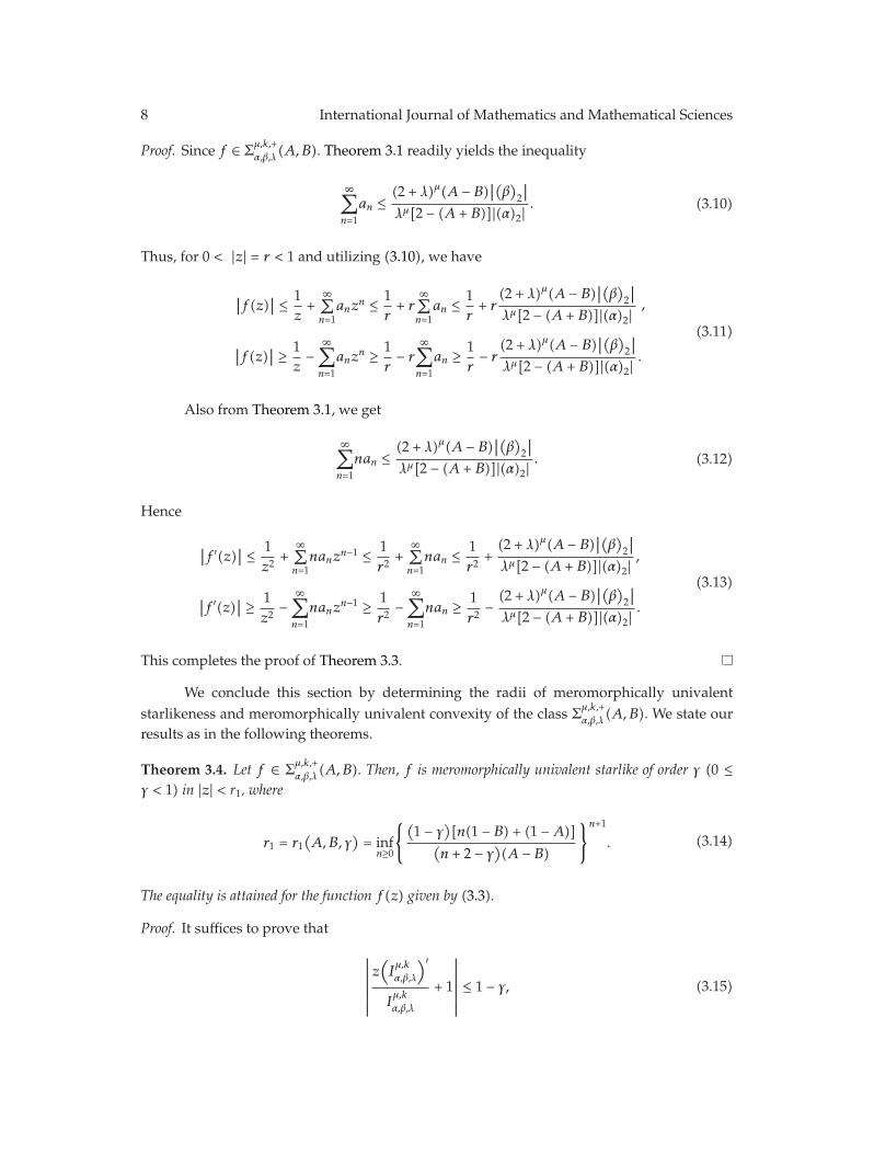
8 International Journal of Mathematics and Mathematical Sciences
Proof. Since f ∈ Σμ,k,+α,β,λ
(A,B). Theorem 3.1 readily yields the inequality
∞∑
n=1
an ≤ (2 + λ)μ(A − B)∣∣(β)2∣∣
λμ[2 − (A + B)]|(α)2|. (3.10)
Thus, for 0 < |z| = r < 1 and utilizing (3.10), we have
∣∣f(z)
∣∣ ≤ 1
z+
∞∑
n=1anz
n ≤ 1r+ r
∞∑
n=1an ≤ 1
r+ r
(2 + λ)μ(A − B)∣∣(β)2∣∣
λμ[2 − (A + B)]|(α)2|,
∣∣f(z)
∣∣ ≥ 1
z−
∞∑
n=1
anzn ≥ 1
r− r
∞∑
n=1
an ≥ 1r− r (2 + λ)
μ(A − B)∣∣(β)2∣∣
λμ[2 − (A + B)]|(α)2|.
(3.11)
Also from Theorem 3.1, we get
∞∑
n=1
nan ≤ (2 + λ)μ(A − B)∣∣(β)2∣∣
λμ[2 − (A + B)]|(α)2|. (3.12)
Hence
∣∣f ′(z)
∣∣ ≤ 1
z2+
∞∑
n=1nanz
n−1 ≤ 1r2
+∞∑
n=1nan ≤ 1
r2+(2 + λ)μ(A − B)∣∣(β)2
∣∣
λμ[2 − (A + B)]|(α)2|,
∣∣f ′(z)
∣∣ ≥ 1
z2−
∞∑
n=1
nanzn−1 ≥ 1
r2−
∞∑
n=1
nan ≥ 1r2
− (2 + λ)μ(A − B)∣∣(β)2∣∣
λμ[2 − (A + B)]|(α)2|.
(3.13)
This completes the proof of Theorem 3.3.
We conclude this section by determining the radii of meromorphically univalentstarlikeness and meromorphically univalent convexity of the class Σμ,k,+
α,β,λ(A,B). We state our
results as in the following theorems.
Theorem 3.4. Let f ∈ Σμ,k,+α,β,λ
(A,B). Then, f is meromorphically univalent starlike of order γ (0 ≤γ < 1) in |z| < r1, where
r1 = r1(A,B, γ
)= inf
n≥0
{(1 − γ)[n(1 − B) + (1 −A)]
(n + 2 − γ)(A − B)
}n+1
. (3.14)
The equality is attained for the function f(z) given by (3.3).
Proof. It suffices to prove that
∣∣∣∣∣∣∣
z(Iμ,k
α,β,λ
)′
Iμ,k
α,β,λ
+ 1
∣∣∣∣∣∣∣
≤ 1 − γ, (3.15)

International Journal of Mathematics and Mathematical Sciences 9
for |z| < r1, we have
∣∣∣∣∣∣∣
z(Iμ,k
α,β,λ
)′
Iμ,k
α,β,λ
+ 1
∣∣∣∣∣∣∣
=
∣∣∣∣∣
∑∞n=1 n
k(n + 1)((α)n+1/
(β)n+1
)(λ/(n + 1 + λ))μanzn
(1/z) +∑∞
n=1 nk((α)n+1/
(β)n+1
)(λ/(n + 1 + λ))μanzn
∣∣∣∣∣
≤∑∞
n=1 nk(n + 1)
(|(α)n+1|/∣∣(β)n+1
∣∣)(λ/(n + 1 + λ))μ|an|
∣∣zn+1
∣∣
1 −∑∞n=1 n
k(|(α)n+1|/
∣∣(β)n+1
∣∣)(λ/(n + 1 + λ))μ|an||zn+1|
.
(3.16)
Hence, (3.16) holds true if
∞∑
n=1
nk(n + 1)|(α)n+1|∣∣(β)n+1
∣∣
(λ
n + 1 + λ
)μ
|an|∣∣∣zn+1
∣∣∣
≤ (1 − γ)
(
1 −∞∑
n=1
nk|(α)n+1|∣∣(β)n+1
∣∣
(λ
n + 1 + λ
)μ
|an|∣∣∣zn+1
∣∣∣
) (3.17)
or
∞∑
n=1
nk(n + 2 − γ1 − γ
) |(α)n+1|∣∣(β)n+1
∣∣
(λ
n + 1 + λ
)μ
|an|∣∣∣zn+1
∣∣∣ ≤ 1, (3.18)
with the aid of (3.18) and (3.2), it is true to have
(nk
(n + 2 − γ)
1 − γ
)|(α)n+1|∣∣(β)n+1
∣∣
(λ
n + 1 + λ
)μ∣∣∣zn+1
∣∣∣
≤ nkλμ[n(1 − B) + (1 −A)]|(α)n+1|(A − B)(n + 1 + λ)μ
∣∣(β)n+1
∣∣
(n ≥ 1).
(3.19)
Solving (3.19) for |z|, we obtain
|z| ≤{(
1 − γ)[n(1 − B) + (1 −A)](n + 2 − γ)(A − B)
}n+1
(n ≥ 1). (3.20)
This completes the proof of Theorem 3.4.
Theorem 3.5. Let f ∈ Σμ,k,+α,β,λ
(A,B). Then, f is meromorphically univalent convex of order γ (0 ≤γ < 1) in |z| < r2, where
r2 = r2(A,B, γ
)= inf
n≥0
{(1 − γ)[nk−1(1 − B) + (1 −A)
]
(n + 2 − γ)(A − B)
}n+1
. (3.21)
The equality is attained for the function f(z) given by (3.3).

10 International Journal of Mathematics and Mathematical Sciences
Proof. By using the technique employed in the proof of Theorem 3.4, we can show that
∣∣∣∣∣∣∣
z(Iμ,k,+α,β,λ
)′′
(Iμ,k,+α,β,λ
)′ + 2
∣∣∣∣∣∣∣
≤ (1 − γ), (3.22)
for |z| < r2, with the aid of Theorem 3.1. Thus, we have the assertion of Theorem 3.5.
Acknowledgment
The work presented here was fully supported by UKM-ST-06-FRGS0244-2010.
References
[1] M. K. Aouf, “On a certain class of meromorphic univalent functions with positive coefficients,”Rendiconti di Matematica e delle sue Applicazioni, vol. 7, no. 11, pp. 209–219, 1991.
[2] S. K. Bajpai, “A note on a class of meromorphic univalent functions,”Revue Roumaine deMathematiquesPures et Appliquees, vol. 22, no. 3, pp. 295–297, 1977.
[3] N. E. Cho, S. H. Lee, and S. Owa, “A class of meromorphic univalent functions with positivecoefficients,” Kobe Journal of Mathematics, vol. 4, no. 1, pp. 43–50, 1987.
[4] B. A. Uralegaddi and M. D. Ganigi, “A certain class of meromorphically starlike functions withpositive coefficients,” Pure and Applied Mathematika Sciences, vol. 26, no. 1-2, pp. 75–81, 1987.
[5] J. Dziok and H. M. Srivastava, “Some subclasses of analytic functions with fixed argumentof coefficients associated with the generalized hypergeometric function,” Advanced Studies inContemporary Mathematics, Kyungshang, vol. 5, no. 2, pp. 115–125, 2002.
[6] J. Dziok and H. M. Srivastava, “Certain subclasses of analytic functions associated with thegeneralized hypergeometric function,” Integral Transforms and Special Functions, vol. 14, no. 1, pp. 7–18,2003.
[7] J.-L. Liu, “A linear operator and its applications on meromorphic p-valent functions,” Bulletin of theInstitute of Mathematics. Academia Sinica, vol. 31, no. 1, pp. 23–32, 2003.
[8] J.-L. Liu and H. M. Srivastava, “A linear operator and associated families of meromorphicallymultivalent functions,” Journal of Mathematical Analysis and Applications, vol. 259, no. 2, pp. 566–581,2001.
[9] J.-L. Liu and H. M. Srivastava, “Certain properties of the Dziok-Srivastava operator,” AppliedMathematics and Computation, vol. 159, no. 2, pp. 485–493, 2004.
[10] J.-L. Liu andH.M. Srivastava, “Classes of meromorphically multivalent functions associated with thegeneralized hypergeometric function,”Mathematical and Computer Modelling, vol. 39, no. 1, pp. 21–34,2004.
[11] N. E. Cho and I. H. Kim, “Inclusion properties of certain classes of meromorphic functions associatedwith the generalized hypergeometric function,” Applied Mathematics and Computation, vol. 187, no. 1,pp. 115–121, 2007.
[12] N. E. Cho, O. S. Kwon, and H. M. Srivastava, “Inclusion and argument properties for certainsubclasses of meromorphic functions associated with a family of multiplier transformations,” Journalof Mathematical Analysis and Applications, vol. 300, no. 2, pp. 505–520, 2004.
[13] J. H. Choi, M. Saigo, and H. M. Srivastava, “Some inclusion properties of a certain family of integraloperators,” Journal of Mathematical Analysis and Applications, vol. 276, no. 1, pp. 432–445, 2002.
[14] K. I. Noor, “On new classes of integral operators,” Journal of Natural Geometry, vol. 16, no. 1-2, pp.71–80, 1999.
[15] K. I. Noor and M. A. Noor, “On Integral Operators,” Journal of Natural Geometry, vol. 238, no. 2, pp.341–352, 1999.
[16] J. Liu, “The Noor integral and strongly starlike functions,” Journal of Mathematical Analysis andApplications, vol. 261, no. 2, pp. 441–447, 2001.

International Journal of Mathematics and Mathematical Sciences 11
[17] J.-L. Liu and K. I. Noor, “Some properties of Noor integral operator,” Journal of Natural Geometry, vol.21, no. 1-2, pp. 81–90, 2002.
[18] F. Ghanim and M. Darus, “Linear operators associated with a subclass of hypergeometricmeromorphic uniformly convex functions,” Acta Universitatis Apulensis., Mathematics, Informatics, no.17, pp. 49–60, 2009.
[19] F. Ghanim, M. Darus, and A. Swaminathan, “New subclass of hypergeometric meromorphicfunctions,” Far East Journal of Mathematical Sciences, vol. 34, no. 2, pp. 245–256, 2009.
[20] K. Piejko and J. Sokoł, “Subclasses of meromorphic functions associated with the Cho-Kwon-Srivastava operator,” Journal of Mathematical Analysis and Applications, vol. 337, no. 2, pp. 1261–1266,2008.
[21] F. Ghanim and M. Darus, “Certain subclasses of meromorphic functions related to Cho-Kwon-Srivastava operator,” Far East Journal of Mathematical Sciences, vol. 48, no. 2, pp. 159–173, 2011.
[22] I. S. Jack, “Functions starlike and convex of order α,” Journal of the London Mathematical Society, vol. 2,no. 3, pp. 469–474, 1971.

Hindawi Publishing CorporationInternational Journal of Mathematics and Mathematical SciencesVolume 2011, Article ID 342895, 7 pagesdoi:10.1155/2011/342895
Research ArticleStability of Admissible Functions
Rabha W. Ibrahim
School of Mathematical Sciences, Faculty of Sciences and Technology, UKM, 43600 Bangi, Malaysia
Correspondence should be addressed to Rabha W. Ibrahim, [email protected]
Received 2 June 2011; Accepted 16 July 2011
Academic Editor: Nak Cho
Copyright q 2011 Rabha W. Ibrahim. This is an open access article distributed under the CreativeCommons Attribution License, which permits unrestricted use, distribution, and reproduction inany medium, provided the original work is properly cited.
By using the concept of the weak subordination, we examine the stability (a class of analyticfunctions in the unit disk is said to be stable if it is closed under weak subordination) for a class ofadmissible functions in complex Banach spaces. The stability of analytic functions in the followingclasses is discussed: Bloch class, little Bloch class, hyperbolic little Bloch class, extend Bloch class(Q p), and Hilbert Hardy class (H 2).
1. Introduction
We denote byU the unit disk {z ∈ C : |z| < 1} and byH(U) the space of all analytic functionsin U. A function I, analytic in U, is said to be an inner function if and only if |I(z)| ≤ 1 suchthat |I(eiθ)| = 1 almost everywhere. We recall that an inner function I can be factored in theform I = BSwhere B is a Blaschke product and S is a singular inner function takes the form
S(z) = exp
(
−∫2π
0
eit + zeit − zdμ(t)
)
, z ∈ U, (1.1)
where μ is a finite positive Lebesgue measure.Let X and Y represent complex Banach spaces. The class of admissible functions
G(X,Y ), consists of those functions f : X → Y that satisfy
∥∥f(x)
∥∥ ≥ 1, when ‖x‖ = 1. (1.2)
If f and g are analytic functions with f, g ∈ G(X,Y ), then f is said to be weaklysubordinate to g, written as f≺wg if there exist analytic functions φ,ω : U → X, with φan inner function (‖φ‖X ≤ 1), so that f ◦ φ = g ◦ω. A class C of analytic functions in X is saidto be stable if it is closed under weak subordination, that is, if f ∈ C whenever f and g areanalytic functions in X with g ∈ C and f≺wg.

2 International Journal of Mathematics and Mathematical Sciences
By making use of the above concept of the weak subordination, we examine thestability for a class of admissible functions in complex Banach spaces G(X,Y ). The stabilityof analytic functions appears in Bloch class, little Bloch class, hyperbolic little Bloch class,extend Bloch class (Qp), and Hilbert Hardy class (H2).
2. Stability of Bloch Classes
If f is an analytic function inU, then f is said to be a Bloch function if
∥∥f
∥∥B =
∣∣f(0)
∣∣ + sup
z∈U
(1 − |z|2
)∣∣f ′(z)
∣∣ <∞. (2.1)
The space of all Bloch functions is denoted by B. The little Bloch space B0 consists of thosef ∈ B such that
lim|z|<1(1 − |z|2
)∣∣f ′(z)
∣∣ = 0. (2.2)
The hyperbolic Bloch class Bh is defined by using the hyperbolic derivative in place of theordinary derivative in the definition of the Bloch space, where the hyperbolic derivative ofan analytic self-map ϕ : U → U of the unit disk is given by |ϕ′|/(1 − |ϕ|2). That is, ϕ ∈ Bh if itis analytic and
supz∈U
(1 − |z|2
)∣∣ϕ′(z)
∣∣
1 − ∣∣ϕ(z)
∣∣2
<∞. (2.3)
Similarly, we say ϕ ∈ Bh0 , the hyperbolic little Bloch class, if ϕ ∈ Bh and
lim|z|=1
(1 − |z|2
)∣∣ϕ′(z)
∣∣
1 − ∣∣ϕ(z)
∣∣2
= 0. (2.4)
Note that, for the function ϕ : U → X, we replace | · | by ‖ · ‖X in the above definitions.
Theorem 2.1. LetX be a complex Banach space. IfX contains all inner functions inU, then G(X,X)is stable.
Proof. Suppose that X contains all inner functions I : U → X. Take g(z) = φ(z) = z andω(z) = I(z) (z ∈ U). Then, φ and ω are inner functions and I = I ◦ φ = g ◦ ω. Hence,I≺wg, g ∈ X, and I ∈ X. Thus, X is stable.
Theorem 2.2. Let X = H(U) be a space of analytic functions in U which satisfies B ⊂ X. Then,G(U,X) is stable.
Proof. Suppose that X = H(U) and B ⊂ X. Let f ∈ X, E = {m + ni : m,n ∈ Z} and F ={z ∈ U : f(z) ∈ E}. Since F is a countable subset of U, it has capacity zero and therefore theuniversal covering map I fromU ontoU \ F is an inner function (see, e.g., Chapter 2 of [1]).Set g = f ◦ I, then the image of g is contained in C/E. Consequently, see [2], g is a Blochfunction. Since B ⊂ X, we have that g = f ◦ I ∈ X even though f ∈ X. Thus, X is stable.

International Journal of Mathematics and Mathematical Sciences 3
Theorem 2.3. Let X = H(U) be a space of analytic functions inU and f ∈ G(X,X). If I : U → Xsatisfying I(0) = Θ (the zero element in X) and ‖f(I(z))‖X < 1, then G(X,X) is stable.
Proof. Assume that X = H(U), f ∈ G(X,X), and I : U → X with I(0) = Θ. Then (see [3])
∥∥f(I(z))
∥∥X < 1 =⇒ ‖I(z)‖X < 1, (2.5)
hence I is an inner function in X. By putting g := f ◦ I, we obtain that g ∈ X even thoughf ∈ X. Thus, X is stable and consequently yields the stability of G(X,X).
Next we discuss the stability of the spaces B0 and Bh0 . An analytic self-map ϕ of U
induces a linear operator Cϕ : H(U) → H(U), defined by Cϕf = f ◦ϕ. This operator is calledthe composition operator induced by ϕ.
Recall that a linear operator T : X → Y is said to be bounded if the image of abounded set in X is a bounded subset of Y , while T is compact if it takes bounded sets tosets with compact closure. Furthermore, if T is a bounded linear operator, then it is calledweakly compact, if T takes bounded sets in X to relatively weakly compact sets in Y . Byusing the operator Cϕf , we have the following result.
Theorem 2.4. If G(B0,B0) is compact, then it is stable.
Proof. Assume the analytic self-map ϕ of U and f ∈ B0; thus, we have the linear operatorCϕ : B0 → B0, defined by Cϕf = f ◦ ϕ := g. By the assumption, we obtain that g is compactfunction in B0. Hence, ϕ is an inner function [4, Corollary 1.3] which implies the stability ofG(B0,B0).
Theorem 2.5. Let ϕ be holomorphic self-map ofU such that
lim|z|=1
(1 − |z|2
)∣∣ϕ′(z)
∣∣
1 − ∣∣ϕ(z)
∣∣2
= 0. (2.6)
Then, G(B0,B0) is stable.
Proof. Assume the analytic self-map ϕ ofU and f ∈ B0; hence, in virtue of [5, Theorem 4.7], itis implied that the composition operator Cϕf on B0 is compact. Thus we pose that G(B0,B0)is stable.
Theorem 2.6. Consider ϕ is a holomorphic self-map ofU, satisfying the following condition: for everyε > 0, there exists 0 < r < 1 such that
(1 − |z|2
)∣∣ϕ′(z)
∣∣
1 − ∣∣ϕ(z)
∣∣2
< ε (2.7)
when |ϕ| > r. Then, G(B0,B0) is stable.

4 International Journal of Mathematics and Mathematical Sciences
Proof. Assume the analytic self-map ϕ of U and f ∈ B0; hence, in virtue of [5, Theorem 4.8],it is yielded that the composition operator Cϕf on B0 is compact. Hence, we obtain thatG(B0,B0) is stable.
Theorem 2.7. If Cϕf is weakly compact in B0, then G(B0,B0) is stable.
Proof. According to [5, Theorem 4.10], we have that Cϕf is compact in B0 and, consequently,G(B0,B0) is stable.
Theorem 2.8. Let ϕ be holomorphic self-map ofU. If the function
τϕ(z) :=
(1 − |z|2
)∣∣ϕ′(z)
∣∣
1 − ∣∣ϕ(z)
∣∣2
(2.8)
is bounded, then G(Bh0 ,Bh
0) is stable.
Proof. Assume the analytic self-map ϕ ofU and f ∈ Bh0 . Since τϕ(z) is bounded, then in virtue
of [4, Theorem 1.2], it is yielded that ϕ is an inner function. By putting g := f ◦ ϕ, whereg ∈ Bh
0 , we have the desired result.
Theorem 2.9. If ϕ ∈ Bh0 , then G(B0,B0) is stable.
Proof. Following [4], it will be shown that there are inner functions ϕ ∈ Bh0 ; then,Cϕ : B0 → B0
is compact (see [4, 5]). Thus, G(B0,B0) is stable.
Theorem 2.10. Let ϕ be self-map in U and w : (0, 1] → (0,∞) be continuous with limt=0w(t) = 0satisfying
lim|z|↑1
(1 − |z|2
)∣∣ϕ′(z)
∣∣
w(1 − ∣
∣ϕ(z)∣∣2) = 0, (2.9)
then G(B0,B0) is stable.
Proof. According to [5, Theorem 5.15], we pose that ϕ is inner. Thus, in view of [4,Corollary 1.3], Cϕ : B0 → B0 is compact; hence, G(B0,B0) is stable.
Remark 2.11. The Schwarz-Pick Lemma implies
(i) Cϕ maps B to B;(ii) 0 ≤ |τϕ(z)| ≤ 1;
(iii) ϕ ∈ B0 if Cϕ maps B0 → B0 and conversely, f, ϕ ∈ B0 ⇒ f ◦ ϕ ∈ B0.
3. Stability of the Hilbert Hardy Space
In this section, we assume that f ∈ H2, whereH2 is the Hilbert Hardy space onU, that is, theset of all analytic functions on U with square summable Taylor coefficients. It is well knownthat each such ϕ (self-map in U) induces a bounded composition operator Cϕf = f ◦ ϕ on

International Journal of Mathematics and Mathematical Sciences 5
H2. Moreover, Joel Shapiro obtained the following characterization of inner functions [6]: thefunction ϕ : U → U is inner if and only if
∥∥Cϕf
∥∥e=
√√√√1 +
∣∣ϕ(0)
∣∣
1 − ∣∣ϕ(0)
∣∣, (3.1)
where |Cϕf |e denotes the essential norm of Cϕf .
Theorem 3.1. Let ϕ be self-map ofU and f ∈ H2. If (1.1) holds, then G(H2,H2) is stable.
Proof. Assume the analytic self-map ϕ of U and f ∈ H2. Condition (1.1) implies that ϕ isan inner function. By setting g := Cϕf = f ◦ ϕ and, consequently, g ∈ H2, it is yielded thatG(H2,H2) is stable.
Next we will show that the compactness of Cϕf introduces the stability of G(H2,H2).Two positive (or complex)measures μ and ν defined on a measurable space (Ω,Σ) are calledsingular if there exist two disjoint sets A and B in Σ whose union is Ω such that μ is zero onall measurable subsets of B while ν is zero on all measurable subsets of A.
Theorem 3.2. If the composition operator Cϕf : H2 → H2 is compact, then G(H2,H2) is stable.
Proof. Since Cϕ : H2 → H2 is compact, all the Aleksandrov measures of ϕ are singularabsolutely continuous with respect to the arc-length measure (see [7, 8]). Thus, in view of[4, Remark 1], ϕ is inner. By letting g := Cϕf = f ◦ ϕ, and, consequently, g ∈ H2, it is yieldedthat G(H2,H2) is stable.
Theorem 3.3. If ϕ has values never approach the boundary ofU, then G(H2,H2) is stable.
Proof. Assume the composition operator Cϕ : H2 → H2. Since ϕ has values never approachthe boundary ofU:
∥∥ϕ
∥∥∞ = sup
{∣∣ϕ
∣∣, z ∈ U}
< 1, (3.2)
Cϕ is compact onH2 (see [9, 10]). Hence, ϕ is an inner function and G(H2,H2) is stable.
Remark 3.4. (i) It is well known that if Cϕ is compact on H2, then it is compact on Hp for all0 < p <∞ (see [9, Theorem 6.1]).
(ii) Cϕ is compact onH∞ if and only if ‖ϕ‖∞ < 1 (see [10, Theorem 2.8]).
Theorem 3.5. If ϕ ∈ Bh0 is univalent then, G(Lpa,Hq), 0 < p < q < ∞ is stable, where Lpa,Hq are
the classical Bergman and Hardy spaces.
Proof. Since ϕ is univalent, Cϕ : Lpa → Hq is compact for all 0 < p < q < ∞
(see [11, Theorem 6.4]). In view of Remark 3.4, we obtain that ϕ is an inner function; hence,G(Lpa,Hq) is stable.
Next, we use the angular derivative criteria to discuss the stability of admissiblefunctions. Recall that ϕ has angular derivative at ζ ∈ ∂U if the nontangential limw = f(ζ) ∈∂U exists and if (f(z) − f(ζ))/(z − ζ) converges to some μ ∈ C as z → ζ nontangentially.

6 International Journal of Mathematics and Mathematical Sciences
Theorem 3.6. If ϕ satisfies both the angular derivative criteria and
sup{nϕ(w) : r < |w| < 1, 0 < r < 1
}<∞, (3.3)
where nϕ(w) is the number of points in ϕ−1(w) with multiplicity counted, then G(H2,H2) is stable.
Proof. According to [12, Corollary 3.6], we have that Cϕ is compact on H2. Again in view ofRemark 3.4, we obtain that ϕ is inner and, consequently, G(H2,H2) is stable.
4. Stability of Qp Class
For 0 < p < 1, an analytic function f inU is said to belong to the space Qp if
supa∈U
∫
U
∣∣f ′(z)
∣∣2g(z, a)pdA(z) <∞, (4.1)
where dA(z) = dxdy = rdrdθ is the Lebesgue areameasure and g denotes the Green functionfor the disk given by
g(z;a) = log1 − aza − z , a, z ∈ U, a/= z. (4.2)
The spaces Qp are conformally invariant. In [13], It was shown that Qp = B for all p, whileQ1 = BMOA, the space of those f ∈ H1 whose boundary values have bounded meanoscillation on ∂U (see [14]). For 0 < α < 1, Λα is the Lipschitz space, consisting of thosef ∈ H(U), which are continuous inU and satisfy
∣∣f(z1) − f(z2)
∣∣ ≤ C|z1 − z2|α, z1, z2 ∈ U, (4.3)
for some C = C(f) > 0. In this section, we will show the stability of functions belong to thespaces Q1 and Λα.
Theorem 4.1. If f ∈ Q1, then G(Q1, Q1) is stable.
Proof. In the similar manner of Theorem 2.2, we pose an inner function ϕ onU. Now, in viewof [15, Theorem H], yields g := f ◦ ϕ ∈ Q1, even though f ∈ Q1. Thus, Q1 is stable.
Theorem 4.2. If f ∈ Λα, 0 < α < 1 such that
∣∣f(z)
∣∣ = O
((1 − |z|)α) (4.4)
for some z, then G(Λα,Λα) is stable.
Proof. Again as in Theorem 2.2, we obtain an inner function ϕ on U. Now in view of [15,Theorem K], yields g := f ◦ ϕ ∈ Λα, even though f ∈ Λα. Thus, Λα is stable.

International Journal of Mathematics and Mathematical Sciences 7
5. Conclusion
From above, we conclude that the composition operator Cϕ, of admissible functions indifferent complex Banach spaces, plays an important role in stability of these spaces. It wasshown that the compactness of this operator implied the stability, when ϕ is an inner functionon the unit disk U. Furthermore, weakly compactness imposed the stability of Bloch spaces.In addition, noncompactness leaded to the stability for some spaces such as Qp-spaces andLipschitz spaces.
References
[1] E. F. Collingwood and A. J. Lohwater, The Theory of Cluster Sets, Cambridge Tracts in Mathematicsand Mathematical Physics, No. 56, Cambridge University Press, Cambridge, UK, 1966.
[2] J. M. Anderson, J. Clunie, and Ch. Pommerenke, “On Bloch functions and normal functions,” Journalfur die Reine und Angewandte Mathematik, vol. 270, pp. 12–37, 1974.
[3] Gr. St. Salagean and H. Wiesler, “Jack’s lemma for holomorphic vector-valued functions,” Cluj.Mathematica, vol. 23(46), no. 1, pp. 85–90, 1981.
[4] W. Smith, “Inner functions in the hyperbolic little Bloch class,” The Michigan Mathematical Journal, vol.45, no. 1, pp. 103–114, 1998.
[5] A. Fletcher, “Bloch functions,” Essay, vol. 3, pp. 1–38, 2002.[6] J. H. Shapiro, “What do composition operators know about inner functions?” Monatshefte fur
Mathematik, vol. 130, no. 1, pp. 57–70, 2000.[7] J. A. Cima and A. L. Matheson, “Essential norms of composition operators and Aleksandrov
measures,” Pacific Journal of Mathematics, vol. 179, no. 1, pp. 59–64, 1997.[8] D. Sarason, Sub-Hardy Hilbert Spaces in the Unit Disk, University of Arkansas Lecture Notes in the
Mathematical Sciences, 10, John Wiley & Sons, New York, NY, USA, 1994.[9] J. H. Shapiro and P. D. Taylor, “Compact, nuclear, and Hilbert-Schmidt composition operators onH2,”
Indiana University Mathematics Journal, vol. 23, pp. 471–496, 1973.[10] H.J. Schwartz, Composition operators on Hp, thesis, Univ. of Toledo, 1969.[11] W. Smith, “Composition operators between Bergman and Hardy spaces,” Transactions of the American
Mathematical Society, vol. 348, no. 6, pp. 2331–2348, 1996.[12] J. H. Shapiro, “The essential norm of a composition operator,” Annals of Mathematics. Second Series,
vol. 125, no. 2, pp. 375–404, 1987.[13] R. Aulaskari and P. Lappan, “Criteria for an analytic function to be Bloch and a harmonic or
meromorphic function to be normal,” in Complex Analysis and Its Applications (Hong Kong, 1993), vol.305 of Pitman Res. Notes Math. Ser., pp. 136–146, Longman Scientic and Technical, Harlow, UK, 1994.
[14] D. Girela, “Analytic functions of bounded mean oscillation,” in Complex Function Spaces (Mekrijarvi,1999), R. Aulaskari, Ed., vol. 4 of Univ. Joensuu Dept. Math. Rep. Ser., pp. 61–170, Univ. Joensuu,Joensuu, Finland, 2001.
[15] J. A. Pelaez, “Inner functions as improving multipliers,” Journal of Functional Analysis, vol. 255, no. 6,pp. 1403–1418, 2008.

Hindawi Publishing CorporationInternational Journal of Mathematics and Mathematical SciencesVolume 2011, Article ID 729849, 9 pagesdoi:10.1155/2011/729849
Research ArticleDomination Conditions for Families ofQuasinearly Subharmonic Functions
Juhani Riihentaus
Department of Mathematical Sciences, University of Oulu, P.O. Box 3000, 90014 Oulun Yliopisto, Finland
Correspondence should be addressed to Juhani Riihentaus, [email protected]
Received 16 February 2011; Accepted 12 April 2011
Academic Editor: Teodor Bulboaca
Copyright q 2011 Juhani Riihentaus. This is an open access article distributed under the CreativeCommons Attribution License, which permits unrestricted use, distribution, and reproduction inany medium, provided the original work is properly cited.
Domar has given a condition that ensures the existence of the largest subharmonic minorant of agiven function. Later Rippon pointed out that a modification of Domar’s argument gives in facta better result. Using our previous, rather general and flexible, modification of Domar’s originalargument, we extend their results both to the subharmonic and quasinearly subharmonic settings.
1. Introduction
1.1. Results of Domar and Rippon
Suppose that D is a domain of �n , n ≥ 2. Let F : D → [0,+∞] be an upper semicontinuousfunction. Let F be a family of subharmonic functions u : D → [0,+∞) which satisfy
u(x) ≤ F(x), (1.1)
for all x ∈ D. Write
w(x) = supu∈F
u(x), x ∈ D, (1.2)
and let w∗ : D → [0,+∞] be the upper semicontinuous regularization of w, that is,
w∗(x) := lim supy→x
w(y). (1.3)

2 International Journal of Mathematics and Mathematical Sciences
Domar gave the following result.
Theorem A. If for some ε > 0,
∫
D
[log+F(x)
]n−1+εdmn(x)< +∞, (1.4)
then w is locally bounded above in D, and thus w∗ is subharmonic in D.
See [1, Theorems 1 and 2, pages 430 and 431]. As Domar points out, the original caseof subharmonic functions in the result of Theorem 1 is due to Sjoberg [2] and Brelot [3] (cf.also [4]). Observe, however, that Domar also sketches a new proof for Theorem 1 which useselementary methods and applies to more general functions.
Rippon [5, Theorem 1, page 128] generalized Domar’s result in the following form.
Theorem B. Let ϕ : [0,+∞] → [0,+∞] be an increasing function such that
∫+∞
1
dt[ϕ(t)]1/(n−1) < +∞. (1.5)
If
∫
D
ϕ(log+F(x)
)dmn(x) < +∞, (1.6)
then w is locally bounded above in D, and thus w∗ is subharmonic in D.
As pointed out by Domar [1, pages 436–440] and by Rippon [5, page 129], the aboveresults are for many particular cases sharp.
As Domar points out, in [1, page 430], the result of his Theorem A holds in fact formore general functions, that is, for functions which by good reasons might be—and indeedalready have been—called quasinearly subharmonic functions. See Section 1.2 below for thedefinition of this function class. In addition, Domar has given a related result for an evenmoregeneral function class K(A, α), where the above conditions (1.4) and (1.6) are replaced by acertain integrability condition on the decreasing rearrangement of logF, see [6, Theorem 1,page 485]. Observe, however, that in the case α = n Domar’s classK(A, n) equals the class ofnonnegative quasinearly subharmonic functions: if u ∈ K(A, n), then u is νnAn+1-quasinearlysubharmonic. Here (and below) νn is the Lebesgue measure of the unit ball Bn(0, 1) in �
n .Conversely, if u ≥ 0 is C-quasinearly subharmonic, then u ∈ K(C, n).
Below we give a general and at the same time flexible result which includes bothDomar’s and Rippon’s results, Theorems A and B above. See Theorem 2.1, Corollary 2.4,and Remark 2.5 below. For previous preliminary, more or less standard results, see also [7,Theorem 2(d), page 15], [8, Theorem 2, page 71], and [9, Theorem 2.2(vi), page 55] (seeRemark 1.2(v)).
Notation. Our notation is rather standard, see, for example, [7, 9]. For the convenience of thereader we, however, recall the following. mn is the Lebesgue measure in the Euclidean space

International Journal of Mathematics and Mathematical Sciences 3
�n , n ≥ 2. D is always a domain in �
n . Constants will be denoted by C and K. They arealways nonnegative and may vary from line to line.
1.2. Subharmonic Functions and Generalizations
We recall that an upper semicontinuous function u : D → [−∞,+∞) is subharmonic if for allclosed balls Bn(x, r) ⊂ D,
u(x) ≤ 1νnrn
∫
Bn(x,r)u(y)dmn
(y). (1.7)
The function u ≡ −∞ is considered subharmonic.We say that a function u : D → [−∞,+∞) is nearly subharmonic, if u is Lebesgue
measurable, u+ ∈ L1loc(D), and for all Bn(x, r) ⊂ D,
u(x) ≤ 1νnrn
∫
Bn(x,r)u(y)dmn
(y). (1.8)
Observe that in the standard definition of nearly subharmonic functions one uses the slightlystronger assumption that u ∈ L1
loc(D), see, for example, [7, page 14]. However, our above,slightly more general definition seems to be more practical, see, for example [9, Propositions2.1(iii) and 2.2(vi)-(vii), pages 54 and 55], and also Remark 1.2(i)–(vi) below. The followinglemma emphasizes this fact still more.
Lemma 1.1 (see [9, Lemma, page 52]). Let u : D → [−∞,+∞) be Lebesgue measurable. Then u isnearly subharmonic (in the sense defined above) if and only if there exists a function u∗, subharmonicin D such that u∗ ≥ u and u∗ = u almost everywhere in D. Here u∗ is the upper semicontinuousregularization of u:
u∗(x) =lim supx′ →x
u(x′). (1.9)
The proof follows at once from [7, proof of Theorem 1, pages 14 and 15], (and referringalso to [9, Propositions 2.1(iii) and 2.2(vii), pages 54 and 55]).
We say that a Lebesgue measurable function u : D → [−∞,+∞) is K-quasinearlysubharmonic, if u+ ∈ L1
loc(D) and if there is a constant K = K(n, u,D) ≥ 1 such that for allBn(x, r) ⊂ D,
uM(x) ≤ K
νnrn
∫
Bn(x,r)uM(y)dmn
(y), (1.10)
for all M ≥ 0, where uM := max{u,−M} +M. A function u : D → [−∞,+∞) is quasinearlysubharmonic, if u is K-quasinearly subharmonic for some K ≥ 1.

4 International Journal of Mathematics and Mathematical Sciences
A Lebesgue measurable function u : D → [−∞,+∞) is K-quasinearly subharmonic n.s.(in the narrow sense), if u+ ∈ L1
loc(D) and if there is a constant K = K(n, u,D) ≥ 1 such that forall Bn(x, r) ⊂ D,
u(x) ≤ K
νnrn
∫
Bn(x,r)u(y)dmn
(y). (1.11)
A function u : D → [−∞,+∞) is quasinearly subharmonic n.s., if u is K-quasinearlysubharmonic n.s. for some K ≥ 1.
As already pointed out, Domar [1, 6] considered nonnegative quasinearly subhar-monic functions. Later on, quasinearly subharmonic functions (perhaps with a differentterminology, and sometimes in certain special cases, or just the corresponding generalizedmean value inequality (1.10) or (1.11)) have been considered in many papers, see, forexample, [8–13] and the references therein.
We recall here only that this function class includes, among others, subharmonicfunctions, and, more generally, quasisubharmonic and nearly subharmonic functions (see,e.g., [7, pages 14 and 26]), also functions satisfying certain natural growth conditions,especially certain eigenfunctions, and polyharmonic functions. Also, the class of Harnackfunctions is included, thus, among others, nonnegative harmonic functions as well asnonnegative solutions of some elliptic equations. In particular, the partial differentialequations associated with quasiregular mappings belong to this family of elliptic equations.
Remark 1.2. For the sake of convenience of the reader we recall the following, see [9,Propositions 2.1 and 2.2, pages 54 and 55].
(i) A K-quasinearly subharmonic function n.s. is K-quasinearly subharmonic, but notnecessarily conversely.
(ii) A nonnegative Lebesgue measurable function isK-quasinearly subharmonic if andonly if it is K-quasinearly subharmonic n.s.
(iii) A Lebesgue measurable function is 1-quasinearly subharmonic if and only if it is1-quasinearly subharmonic n.s. and if and only if it is nearly subharmonic (in thesense defined above).
(iv) If u : D → [−∞,+∞) is K1-quasinearly subharmonic and v : D → [−∞,+∞) isK2-quasinearly subharmonic, then max{u, v} is max{K1, K2}-quasinearly subhar-monic in D. Especially, u+ := max{u, 0} is K1-quasinearly subharmonic in D.
(v) LetF be a family ofK-quasinearly subharmonic (resp.,K-quasinearly subharmonicn.s.) functions in D and let w := supu∈Fu. If w is Lebesgue measurable and w+ ∈L1
loc(D), then w is K-quasinearly subharmonic (resp., K-quasinearly subharmonicn.s.) in D.
(vi) If u : D → [−∞,+∞) is quasinearly subharmonic n.s., then either u ≡ −∞ or u isfinite almost everywhere inD, and u ∈ L1
loc(D).
2. The Result
Theorem 2.1. LetK ≥ 1. Let ϕ : [0,+∞] → [0,+∞] and let ψ : [0,+∞] → [0,+∞] be increasingfunctions for which there are s0, s1 ∈ �, s0 < s1, such that

International Journal of Mathematics and Mathematical Sciences 5
(i) the inverse functions ϕ−1 and ψ−1 are defined on [min{ϕ(s1 − s0), ψ(s1 − s0)},+∞],
(ii) 2K(ψ−1 ◦ ϕ)(s − s0) ≤ (ψ−1 ◦ ϕ)(s) for all s ≥ s1,(iii) the function
[s1 + 1,+∞] � s −→(ψ−1 ◦ ϕ)(s + 1)(ψ−1 ◦ ϕ)(s) ∈ � (2.1)
is bounded,
(iv) the following integral is convergent:
∫+∞
s1
ds
ϕ(s − s0)1/(n−1)< +∞. (2.2)
Let FK be a family of K-quasinearly subharmonic functions u : D → [−∞,+∞) such that
u(x) ≤ FK(x), (2.3)
for all x ∈ D, where FK : D → [0,+∞] is a Lebesgue measurable function. If for each compact setE ⊂ D,
∫
E
ψ(FK(x))dmn(x) < +∞, (2.4)
then the family FK is locally (uniformly) bounded in D. Moreover, the function w∗ : D → [ 0,+∞)is aK-quasinearly subharmonic function. Here
w∗(x) := lim supy→x
w(y), (2.5)
where
w(x) := supu∈FK
u+(x). (2.6)
The proof of the theoremwill be based on the following lemma, which has its origin in[1, Lemma 1, pages 431 and 432], see also [14, Proposition 2, pages 257–259]. Observe that wehave applied our rather general and flexible lemma already before (unlike previously, nowwe allow also the value +∞ for our “test functions” ϕ and ψ; this does not, however, causeany changes in the proof of our lemma, see [15, pages 5–8]) when considering quasinearlysubharmonicity of separately quasinearly subharmonic functions. As a matter of fact, thislemma enabled us to slightly improve Armitage’s and Gardiner’s almost sharp condition,see [14, Theorem 1, page 256], which ensures a separately subharmonic function to besubharmonic. See [15, Corollary 4.5, page 13], and [12, 13, Corollary 3.3.3, page 2622].

6 International Journal of Mathematics and Mathematical Sciences
Lemma 2.2 (see [15, Lemma 3.2, page 5 and Remark 3.3, page 8]). Let K, ϕ, ψ and s0, s1 ∈ �
be as in Theorem 2.1. Let u : D → [ 0,+∞) be a K-quasinearly subharmonic function. Let s1 ∈ �,s1 ≥ s3, be arbitrary, where s3 := max{s1 + 3, (ψ−1 ◦ϕ)(s1 + 3)}. Then for each x ∈ D and r > 0 such
that Bn(x, r) ⊂ D either
u(x) ≤(ψ−1 ◦ ϕ
)(s1 + 1) (2.7)
or
Φ(u(x)) ≤ C
rn
∫
Bn(x,r)ψ(u(y))dmn
(y), (2.8)
where C = C(n,K, s0) and Φ : [ 0,+∞) → [0,+∞),
Φ(t) :=
⎧⎪⎪⎪⎪⎪⎨
⎪⎪⎪⎪⎪⎩
[∫+∞
(ϕ−1◦ψ)(t)−2
ds
ϕ(s − s0)1/(n−1)]1−n
, when t ≥ s3,
t
s3Φ(s3), when 0 ≤ t < s3.
(2.9)
Proof of Theorem 2.1. Let E be an arbitrary compact subset of D. Write ρ0 := dist(E, ∂D).Clearly ρ0 > 0. Write
E1 :=⋃
x∈EBn(x,ρ02
). (2.10)
Then E1 is compact, and E ⊂ E1 ⊂ D. Take u ∈ F+K arbitrarily, where
F+K := {u+ : u ∈ FK}. (2.11)
Let s1 = s1 + 2, say. Take x ∈ E arbitrarily and suppose that u(x) > s3, where s3 := max{s1 +3, (ψ−1 ◦ ϕ)(s1 + 3)}, say. Using our lemma and the assumption, we get
(∫+∞
(ϕ−1◦ψ)(u(x))−2
ds
ϕ(s − s0)1/(n−1))1−n
≤ C(ρ0/2
)n
∫
Bn(x,ρ0/2)ψ(u(y))dmn
(y)
≤ C(ρ0/2
)n
∫
E1
ψ(FK(y))dmn
(y)< +∞.
(2.12)
Since
∫+∞
s1
ds
ϕ(s − s0)1/(n−1)< +∞, (2.13)

International Journal of Mathematics and Mathematical Sciences 7
and 1 − n < 0, the set of values
(ϕ−1 ◦ ψ
)(u(x)) − 2, x ∈ E, u ∈ F+
K, (2.14)
is bounded. Thus also the set of values
u(x), x ∈ E, u ∈ F+K, (2.15)
is bounded.To show that w∗ is K-quasinearly subharmonic in D, proceed as follows. Take x ∈ D
and r > 0 such that Bn(x, r) ⊂ D. For each u ∈ F+K we have then
u(x) ≤ K
νnrn
∫
Bn(x,r)u(y)dmn
(y). (2.16)
Since
u(x) ≤ supu∈F+
K
u(x) = w(x) ≤ w∗(x), (2.17)
we have
w(x) ≤ K
νnrn
∫
Bn(x,r)w∗(y
)dmn
(y). (2.18)
Then just take the upper semicontinuous regularizations on both sides of (2.18) anduse Fatou’s lemma on the right-hand side (this is of course possible, since w∗ is locallybounded in D), say
lim supy→x
w(y) ≤ lim sup
y→x
K
νnrn
∫
Bn(y,r)w∗(z)dmn(z)
≤ lim supy→x
K
νnrn
∫
w∗(z)χBn(y,r)(z)dmn(z)
≤ K
νnrn
∫
w∗(z)
(
lim supy→x
χBn(y,r)(z)
)
dmn(z).
(2.19)
Since for all z ∈ D,
lim supy→ x
χBn(y,r)(z) ≤ χBn(x,r)(z), (2.20)

8 International Journal of Mathematics and Mathematical Sciences
we get the desired inequality
w∗(x) ≤ K
νnrn
∫
Bn(x,r)w∗(y
)dmn
(y). (2.21)
Remark 2.3. If w is Lebesgue measurable, it follows that already w is K-quasinearlysubharmonic.
Corollary 2.4. Let ϕ : [0,+∞] → [0,+∞] be a strictly increasing function such that for somes0, s1 ∈ �, s0 < s1,
∫+∞
s1
ds[ϕ(s − s0)
]1/(n−1) < +∞. (2.22)
Let FK be a family of K-quasinearly subharmonic functions u : D → [−∞,+∞) such that
u(x) ≤ FK(x), (2.23)
for all x ∈ D, where FK : D → [0,+∞] is a Lebesgue measurable function.Let p > 0 be arbitrary. If for each compact set E ⊂ D,
∫
E
ϕ(log+[F(x)]p
)dmn(x) < +∞, (2.24)
then the family FK is locally (uniformly) bounded in D. Moreover, the function w∗ : D → [ 0,+∞)is aK-quasinearly subharmonic function. Here
w∗(x) := lim supy→x
w(y), (2.25)
wherew(x) := sup
u∈FK
u+(x). (2.26)
The case p = 1 and K = 1 gives Domar’s and Rippon’s results, Theorems A and Babove. For the proof, take p > 0 arbitrarily, choose ψ(t) = (ϕ ◦ log+)(tp), and just check thatthe conditions (i)–(iv) indeed hold.
Remark 2.5. As already pointed out, Theorem 2.1 is indeed flexible. To get another simple,but still slightly more general corollary, just choose, say, ψ(t) = (ϕ ◦ log+)(φ(t)), whereφ : [0,+∞] → [0,+∞] is any strictly increasing function which satisfies the following twoconditions:
(a) φ−1 satisfies the Δ2-condition,
(b) 2Kφ−1(es−s0) ≤ φ−1(es) for all s ≥ s1.

International Journal of Mathematics and Mathematical Sciences 9
References
[1] Y. Domar, “On the existence of a largest subharmonic minorant of a given function,” Arkiv forMatematik, vol. 3, no. 39, pp. 429–440, 1957.
[2] N. Sjoberg, “Sur les minorantes sousharmoniques d’une fonction donnee,” in Neuvieme Congres desmathematiciens Scandinaves, pp. 309–319, Helsingfors, 1938.
[3] M. Brelot, “Minorantes sous-harmoniques, extremales et capacites,” Journal de Mathematiques Pures etAppliquees. Neuvieme Serie, vol. 24, pp. 1–32, 1945.
[4] J. W. Green, “Approximately subharmonic functions,” Proceedings of the American Mathematical Society,vol. 3, pp. 829–833, 1952.
[5] P. J. Rippon, “Some remarks on largest subharmonic minorants,” Mathematica Scandinavica, vol. 49,no. 1, pp. 128–132, 1981.
[6] Y. Domar, “Uniform boundedness in families related to subharmonic functions,” Journal of the LondonMathematical Society. Second Series, vol. 38, no. 3, pp. 485–491, 1988.
[7] M. Herve, Analytic and Plurisubharmonic Functions in Finite and Infinite Dimensional Spaces, LectureNotes in Mathematics, Vol. 198, Springer, Berlin, Germany, 1971.
[8] J. Riihentaus, “On a theorem of Avanissian-Arsove,” Expositiones Mathematicae, vol. 7, no. 1, pp. 69–72,1989.
[9] J. Riihentaus, “Subharmonic functions, generalizations and separately subharmonic functions,” inXIV Conference on Analytic Functions, vol. 2 of Scientific Bulletin of Chełm, Section of Mathematics andComputer Science, pp. 49–76, Chełm, Poland, 2007.
[10] M. Pavlovic, “On subharmonic behaviour and oscillation of functions on balls in �n ,” Institut
Mathematique. Publications. Nouvelle Serie, vol. 55(69), pp. 18–22, 1994.[11] M. Pavlovic and J. Riihentaus, “Classes of quasi-nearly subharmonic functions,” Potential Analysis,
vol. 29, no. 1, pp. 89–104, 2008.[12] J. Riihentaus, “Subharmonic functions, generalizations, weighted boundary behavior, and separately
subharmonic functions: A survey,” in 5th World Congress of Nonlinear Analysts (WCNA ’08), Orlando,Fla, USA, 2008.
[13] J. Riihentaus, “Subharmonic functions, generalizations, weighted boundary behavior, and separatelysubharmonic functions: A survey,”Nonlinear Analysis, Series A: Theory, Methods & Applications, vol. 71,no. 12, pp. e2613–e26267, 2009.
[14] D. H. Armitage and S. J. Gardiner, “Conditions for separately subharmonic functions to besubharmonic,” Potential Analysis, vol. 2, no. 3, pp. 255–261, 1993.
[15] J. Riihentaus, “Quasi-nearly subharmonicity and separately quasi-nearly subharmonic functions,”Journal of Inequalities and Applications, vol. 2008, Article ID 149712, 15 pages, 2008.

Hindawi Publishing CorporationInternational Journal of Mathematics and Mathematical SciencesVolume 2011, Article ID 834064, 9 pagesdoi:10.1155/2011/834064
Research ArticleOn Starlike and Convex Functions with Respect tok-Symmetric Points
Afaf A. Ali Abubaker and Maslina Darus
School of Mathematical Sciences, Faculty of Science and Technology, Universiti Kebangsaan Malaysia,Bangi, 43600 Selangor, Malaysia
Correspondence should be addressed to Maslina Darus, [email protected]
Received 29 January 2011; Revised 13 March 2011; Accepted 19 March 2011
Academic Editor: Stanisława R. Kanas
Copyright q 2011 A. A. A. Abubaker and M. Darus. This is an open access article distributedunder the Creative Commons Attribution License, which permits unrestricted use, distribution,and reproduction in any medium, provided the original work is properly cited.
We introduce new subclasses Sσ,sk(λ, δ, φ) and Kσ,s
k(λ, δ, φ) of analytic functions with respect to k-
symmetric points defined by differential operator. Some interesting properties for these classes areobtained.
1. Introduction
Let A denote the class of functions of the form
f(z) = z +∞∑
n=2
anzn, (1.1)
which are analytic in the unit diskU = {z ∈ � : |z| < 1}.Also let ℘ be the class of analytic functions p with p(0) = 1, which are convex and
univalent inU and satisfy the following inequality:
�{p(z)}> 0, z ∈ U. (1.2)
A function f ∈ A is said to be starlike with respect to symmetrical points inU if it satisfies
�
{zf ′(z)
f(z) − f(−z)}
> 0, z ∈ U. (1.3)

2 International Journal of Mathematics and Mathematical Sciences
This class was introduced and studied by Sakaguchi in 1959 [1]. Some related classes arestudied by Shanmugam et al. [2].
In 1979, Chand and Singh [3] defined the class of starlike functions with respect tok-symmetric points of order α (0 ≤ α < 1). Related classes are also studied by Das and Singh[4].
Recall that the function F is subordinate to G if there exists a function ω, analytic inU,with ω(0) = 0 and |ω(z)| < 1, such that F(z) = G(w(z)), z ∈ U. We denote this subordinationby F(z) ≺ G(z). If G(z) is univalent inU, then the subordination is equivalent to F(0) = G(0)and F(U) ⊂ G(U).
A function f ∈ A is in the class Sk(φ) satisfying
zf ′(z)fk(z)
≺ φ(z), z ∈ U, (1.4)
where φ ∈ ℘, k is a fixed positive integer, and fk(z) is given by the following:
fk(z) =1k
k−1∑
ν=0
ε−νf(ενz)
= z +∞∑
ι=2
ak(ι−1)+1zk(ι−1)+1,(
ε = exp(2πik
)
, z ∈ U)
.
(1.5)
The classes Sk(φ) of starlike functions with respect to k-symmetric points and Kk(φ) ofconvex functions with respect to k-symmetric points were considered recently by Wang et al.[5]. Moreover, the special case
φ(z) =1 + βz1 − αβz , 0 ≤ α ≤ 1, 0 < β ≤ 1 (1.6)
imposes the class Sk(α, β), which was studied by Gao and Zhou [6], and the class S1(φ) =S∗(φ) was studied by Ma and Minda [7].
Let two functions given by f(z) = z +∑∞
n=2 anzn and g(z) = z +
∑∞n=2 bnz
n be analyticin U. Then the Hadamard product (or convolution) f ∗ g of the two functions f , g is definedby
f(z) ∗ g(z) = z +∞∑
n=2
anbnzn, (1.7)
and for several function f1(z), . . . , fm(z) ∈ A,
f1(z) ∗ · · · ∗ fm(z) = z +∞∑
n=2(a1n · · ·amn)zn, z ∈ U. (1.8)
The theory of differential operators plays important roles in geometric function theory.Perhaps, the earliest study appeared in the year 1900, and since then, many mathematicianshave worked extensively in this direction. For recent work see, for example, [8–12].

International Journal of Mathematics and Mathematical Sciences 3
We now define differential operator as follows:
Dσ,sλ,δf(z) = z +
∞∑
n=2
ns(C(δ, n)[1 + λ(n − 1)])σanzn, (1.9)
where λ ≥ 0, C(δ, n) = (δ + 1)n−1/(n − 1)!, for δ, σ, s ∈ N0 = {0, 1, 2, . . .}, and (x)n is thePochhammer symbol defined by
(x)n =Γ(x + n)Γ(x)
=
⎧⎨
⎩
1, n = 0,
x(x + 1) · · · (x + n − 1), n = {1, 2, 3, . . .}.(1.10)
HereDσ,sλ,δf(z) can also be written in terms of convolution as
ψ(z) =
[λz
(1 − z)2− λz
1 − z +z
1 − z
]
∗ z
(1 − z)δ+1, z ∈ U,
Dσ,sλ,δf(z) = ψ(z) ∗ · · · ∗ ψ(z)
︸ ︷︷ ︸σ-times
∗∞∑
n=1
nszn ∗ f(z) = Dδ ∗ · · · ∗Dδ︸ ︷︷ ︸σ-times
∗Dσ,sλf(z),
(1.11)
where Dδ = z +∑∞
n=2 C(δ, n)zn andDσ,s
λ= z +
∑∞n=2 n
s[1 + λ(n − 1)]σzn.Note that D0,1
λ,δf(z) = D1,0
1,0f(z) = z f ′(z) and D0,0λ,δf(z) = f(z). When σ = 0, we get the
Sulugean differential operator [9], when λ = s = 0, σ = 1 we obtain the Ruscheweyh operator[8], when s = 0, σ = 1, we obtain the Al-Shaqsi and Darus [11], and when δ = s = 0, weobtain the Al-Oboudi differential operator [10].
In this paper, we introduce new subclasses of analytic functions with respect to k-symmetric points defined by differential operator. Some interesting properties of Sσ,s
k(λ, δ, φ)
and Kσ,sk(λ, δ, φ) are obtained.
Applying the operator Dσ,sλ,δf(z)
Dσ,sλ,δfk(z) =
1k
k−1∑
ν=0
ε−νDσ,sλ,δf(ε
νz), εk = 1, (1.12)
where k is a fixed positive integer, we now define classes of analytic functions containing thedifferential operator.
Definition 1.1. Let Sσ,sk (λ, δ, φ) denote the class of functions in A satisfying the condition
z(Dσ,sλ,δf(z))′
Dσ,sλ,δfk(z)
≺ φ(z), (1.13)
where φ ∈ ℘.

4 International Journal of Mathematics and Mathematical Sciences
Definition 1.2. Let Kσ,sk(λ, δ, φ) denote the class of functions in A satisfying the condition
(
z(Dσ,sλ,δf(z)
)′)′
(Dσ,sλ,δfk(z)
)′ ≺ φ(z), (1.14)
where φ ∈ ℘.
In order to prove our results, we need the following lemmas.
Lemma 1.3 (see [13]). Let c > −1, and let Ic : A → A be the integral operator defined by F = Ic(f),where
F(z) =c + 1zc
∫z
0tc−1f(t)dt. (1.15)
Let φ be a convex function, with φ(0) = 1 and �{φ(z) + c} > 0 in U. If f ∈ A and zf ′(z)/f(z) ≺φ(z), then zF ′(z)/F(z) ≺ q(z) ≺ φ(z), where q is univalent and satisfies the differential equation
q(z) +zq′(z)q(z) + c
= φ(z). (1.16)
Lemma 1.4 (see [14]). Let κ, υ be complex numbers. Let φ be convex univalent in U with φ(0) = 1and �[κφ + υ] > 0, z ∈ U, and let q(z) ∈ A with q(0) = 1 and q(z) ≺ φ(z). If p(z) = 1 + p1z +p2z2 + · · · ∈ ℘ with p(0) = 1, then
p(z) +zp′(z)
κq(z) + υ≺ φ(z) =⇒ p(z) ≺ φ(z). (1.17)
Lemma 1.5 (see [15]). Let f and g, respectively, be in the classes convex function and starlikefunction. Then, for every functionH ∈ A, one has
(f(z) ∗ g(z)H(z)
)
f(z) ∗ g(z) ∈ co(H(U)), z ∈ U, (1.18)
where co(H(U)) denotes the closed convex hull ofH(U).
2. Main Results
Theorem 2.1. Let f ∈ Sσ,sk (λ, δ, φ). Then fk defined by (1.5) is in Sσ,s1 (λ, δ, φ) = Sσ,s(λ, δ, φ).
Proof. Let f ∈ Sσ,sk(λ, δ, φ), then by Definition 1.1 we have
z(Dσ,sλ,δf(z))′
Dσ,sλ,δfk(z)
≺ φ(z). (2.1)

International Journal of Mathematics and Mathematical Sciences 5
Substituting z by ενz, where εk = 1 (ν = 0, 1, . . . , k − 1) in (2.1), respectively, we have
ενz(Dσ,sλ,δf(ενz)
)′
Dσ,sλ,δfk(ε
νz)≺ φ(z). (2.2)
According to the definition of fk and εk = 1, we know fk(ενz) = ενfk(z) for any ν = 0, 1, . . . ,k − 1, and summing up, we can get
1k
k−1∑
ν=0
ε−ν
⎡
⎢⎣z(Dσ,sλ,δf( ενz )
)′
Dσ,sλ,δfk(z)
⎤
⎥⎦ =
z[(1/k)
∑k−1ν=0 ε
−νDσ,sλ,δf(ενz)
]′
Dσ,sλ,δfk(z)
=z(Dσ,sλ,δfk(z)
)′
Dσ,sλ,δfk(z)
. (2.3)
Hence there exist ζν inU such that
z(Dσ,sλ,δfk(z)
)′
Dσ,sλ,δfk(z)
=1k
k−1∑
ν=0
φ(ζν) = φ(ζ0), (2.4)
for ζ0 ∈ U since φ(U) is convex. Thus fk ∈ Sσ,s(λ, δ, φ).
Theorem 2.2. Let f ∈ A and φ ∈ ℘. Then
f ∈ Kσ,sk
(λ, δ, φ
)⇐⇒ zf ′ ∈ Sσ,sk
(λ, δ, φ
). (2.5)
Proof. Let
g(z) = z +∞∑
n=2
ns(C(δ, n)[1 + λ(n − 1)])σzn, (2.6)
and the operatorDσ,sλ,δf can be written as Dσ,s
λ,δf = g ∗ f .
Then from the definition of the differential operatorDσ,sλ,δ, we can verify
(
z(Dσ,sλ,δf(z))′)′
(Dσ,sλ,δfk(z)
)′ =
(z(g ∗ f)′
)′(z)
(g ∗ f)′
k(z)=z(g ∗ zf ′)′(z)(g ∗ zf ′)
k(z)=z(Dσ,sλ,δzf ′(z)
)′
Dσ,sλ,δzf ′
k(z). (2.7)
Thus f ∈ Kσ,sk(λ, δ, φ) if and only if zf ′ ∈ Sσ,s
k(λ, δ, φ).
By using Theorems 2.2 and 2.1, we get the following.
Corollary 2.3. Let f ∈ Kσ,sk(λ, δ, φ). Then fk defined by (1.5) is in Kσ,s
1 (λ, δ, φ) = Kσ,s(λ, δ, φ).
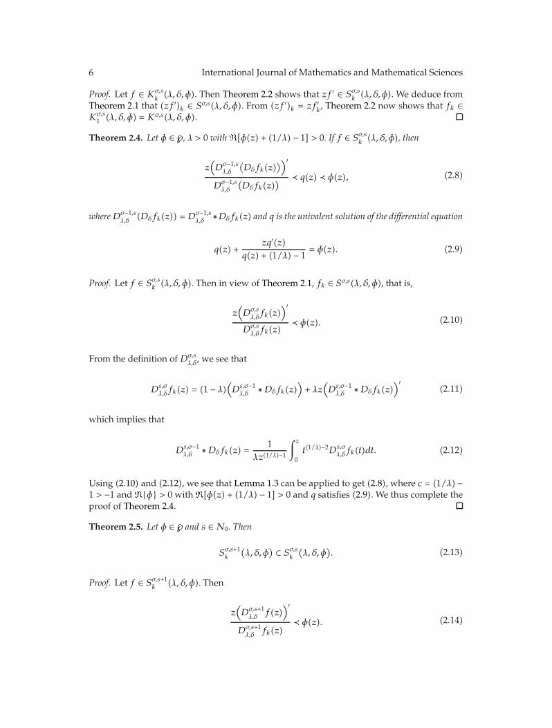
6 International Journal of Mathematics and Mathematical Sciences
Proof. Let f ∈ Kσ,sk(λ, δ, φ). Then Theorem 2.2 shows that zf ′ ∈ Sσ,s
k(λ, δ, φ). We deduce from
Theorem 2.1 that (zf ′)k ∈ Sσ,s(λ, δ, φ). From (zf ′)k = zf ′k, Theorem 2.2 now shows that fk ∈
Kσ,s1 (λ, δ, φ) = Kσ,s(λ, δ, φ).
Theorem 2.4. Let φ ∈ ℘, λ > 0 with�[φ(z) + (1/λ) − 1] > 0. If f ∈ Sσ,sk (λ, δ, φ), then
z(Dσ−1,sλ,δ
(Dδfk(z)
))′
Dσ−1,sλ,δ
(Dδfk(z)
) ≺ q(z) ≺ φ(z), (2.8)
whereDσ−1,sλ,δ
(Dδfk(z)) = Dσ−1,sλ,δ
∗Dδfk(z) and q is the univalent solution of the differential equation
q(z) +zq′(z)
q(z) + (1/λ) − 1= φ(z). (2.9)
Proof. Let f ∈ Sσ,sk (λ, δ, φ). Then in view of Theorem 2.1, fk ∈ Sσ,s(λ, δ, φ), that is,
z(Dσ,sλ,δfk(z)
)′
Dσ,sλ,δfk(z)
≺ φ(z). (2.10)
From the definition of Dσ,sλ,δ
, we see that
Ds,σλ,δfk(z) = (1 − λ)
(Ds,σ−1λ,δ ∗Dδfk(z)
)+ λz(Ds,σ−1λ,δ ∗Dδfk(z)
)′(2.11)
which implies that
Ds,σ−1λ,δ
∗Dδfk(z) =1
λz(1/λ)−1
∫z
0t(1/λ)−2Ds,σ
λ,δfk(t)dt. (2.12)
Using (2.10) and (2.12), we see that Lemma 1.3 can be applied to get (2.8), where c = (1/λ) −1 > −1 and �{φ} > 0 with �[φ(z) + (1/λ) − 1] > 0 and q satisfies (2.9). We thus complete theproof of Theorem 2.4.
Theorem 2.5. Let φ ∈ ℘ and s ∈N0. Then
Sσ,s+1k
(λ, δ, φ
) ⊂ Sσ,sk
(λ, δ, φ
). (2.13)
Proof. Let f ∈ Sσ,s+1k (λ, δ, φ). Then
z(Dσ,s+1λ,δ
f(z))′
Dσ,s+1λ,δ
fk(z)≺ φ(z). (2.14)

International Journal of Mathematics and Mathematical Sciences 7
Set
p(z) =z(Dσ,sλ,δf(z))′
Dσ,sλ,δfk(z)
, (2.15)
where p is analytic function with p(0) = 1. By using the equation
z(Dσ,sλ,δf(z)
)′= Dσ,s+1
λ,δ f(z), (2.16)
we get
p(z) =Dσ,s+1λ,δ
f(z)
Dσ,sλ,δfk(z)
(2.17)
and then differentiating, we get
z(Dσ,s+1λ,δ f(z)
)′= zDσ,s
λ,δfk(z)p′(z) + z
(Dσ,sλ,δfk(z)
)′p(z), (2.18)
Hence
z(Dσ,s+1λ,δ
f(z))′
Dσ,s+1λ,δ fk(z)
=Dσ,sλ,δfk(z)
Dσ,s+1λ,δ fk(z)
zp′(z) +z(Dσ,sλ,δfk(z)
)′
Dσ,s+1λ,δ fk(z)
p(z). (2.19)
Applying (2.16) for the function fk we obtain
z(Dσ,s+1λ,δ f(z)
)′
Dσ,s+1λ,δ
fk(z)=
Dσ,sλ,δfk(z)
Dσ,s+1λ,δ
fk(z)zp′(z) + p(z). (2.20)
Using (2.20) with q(z) = (Dσ,s+1λ,δ
fk(z))/(Dσ,sλ,δfk(z)), we obtain
z(Dσ,s+1λ,δ
f(z))′
Dσ,s+1λ,δ
fk(z)=zp′(z)q(z)
+ p(z). (2.21)
Since f ∈ Sσ,s+1k
(λ, δ, φ), then by using (2.14) in (2.21) we get the following.
zp′(z)q(z)
+ p(z) ≺ φ(z). (2.22)
We can see that q(z) ≺ φ(z), hence applying Lemma 1.4 we obtain the required result.
By using Theorems 2.2 and 2.5, we get the following.

8 International Journal of Mathematics and Mathematical Sciences
Corollary 2.6. Let φ ∈ ℘ and s ∈ N0. Then
Kσ,s+1k
(λ, δ, φ
) ⊂ Kσ,sk
(λ, δ, φ
). (2.23)
Now we prove that the class Sσ,sk (λ, δ, φ), φ ∈ ℘, is closed under convolution withconvex functions.
Theorem 2.7. Let f ∈ Sσ,sk(λ, δ, φ), φ ∈ ℘, and ϕ is a convex function with real coefficients in U.
Then f ∗ ϕ ∈ Sσ,sk(λ, δ, φ).
Proof. Let f ∈ Sσ,sk (λ, δ, φ), then Theorem 2.1 asserts that Dσ,sλ,δfk(z) ∈ S∗(φ), where �{φ} > 0.
Applying Lemma 1.5 and the convolution properties we get
z(Dσ,sλ,δ
(f ∗ ϕ)(z)
)′
Dσ,sλ,δ
(fk ∗ ϕ
)(z)
=z(Dσ,sλ,δf(z) ∗ ϕ(z)
)′
ϕ(z) ∗Dσ,sλ,δfk(z)
=ϕ(z) ∗
(
z(Dσ,sλ,δf(z))′/fDσ,s
λ,δfk(z)
)
Dσ,sλ,δfk(z)
ϕ(z) ∗Dσ,sλ,δfk(z)
∈ co
⎛
⎜⎝z(Dσ,sλ,δf)′
Dσ,sλ,δfk
(U)
⎞
⎟⎠ ⊆ φ(U).
(2.24)
Corollary 2.8. Let f ∈ Kσ,sk(λ, δ, φ), φ ∈ ℘, and ϕ is a convex function with real coefficients in U.
Then f ∗ ϕ ∈ Kσ,sk(λ, δ, φ).
Proof. Let f ∈ Kσ,sk (λ, δ, φ), φ ∈ ℘. Then Theorem 2.2 shows that zf ′ ∈ Sσ,sk (λ, δ, φ). The result
of Theorem 2.7 yields (zf ′) ∗ ϕ = z(f ∗ ϕ)′ ∈ Sσ,sk (λ, δ, φ), and thus f ∗ ϕ ∈ Kσ,sk (λ, δ, φ).
Some other works related to other differential operators with respect to symmetricpoints for different types of problems can be seen in ([16–21]).
Acknowledgments
The work presented here was partially supported by UKM-ST-06-FRGS0244-2010, and theauthors would like to thank the anonymous referees for their informative and criticalcomments on the paper.
References
[1] K. Sakaguchi, “On a certain univalent mapping,” Journal of the Mathematical Society of Japan, vol. 11,pp. 72–75, 1959.
[2] T. N. Shanmugam, C. Ramachandran, and V. Ravichandran, “Fekete-Szego problem for subclasses ofstarlike functions with respect to symmetric points,” Bulletin of the Korean Mathematical Society, vol.43, no. 3, pp. 589–598, 2006.

International Journal of Mathematics and Mathematical Sciences 9
[3] R. Chand and P. Singh, “On certain schlicht mappings,” Indian Journal of Pure and Applied Mathematics,vol. 10, no. 9, pp. 1167–1174, 1979.
[4] R. N. Das and P. Singh, “On subclasses of schlicht mapping,” Indian Journal of Pure and AppliedMathematics, vol. 8, no. 8, pp. 864–872, 1977.
[5] Z.-G. Wang, C.-Y. Gao, and S.-M. Yuan, “On certain subclasses of close-to-convex and quasi-convexfunctions with respect to k-symmetric points,” Journal of Mathematical Analysis and Applications, vol.322, no. 1, pp. 97–106, 2006.
[6] C. Gao and S. Zhou, “A new subclass of close-to-convex functions,” Soochow Journal of Mathematics,vol. 31, no. 1, pp. 41–49, 2005.
[7] W. C. Ma and D. Minda, “A unified treatment of some special classes of univalent functions,” inProceedings of the Conference on Complex Analysis, pp. 157–169.
[8] S. Ruscheweyh, “New criteria for univalent functions,” Proceedings of the American MathematicalSociety, vol. 49, pp. 109–115, 1975.
[9] G. Salagean, “Subclasses of univalent functions,” in Complex Analysis—Fifth Romanian-FinnishSeminar, vol. 1013 of Lecture Notes in Mathematics, pp. 362–372, Springer, Berlin, Germany, 1983.
[10] F. M. Al-Oboudi, “On univalent functions defined by a generalized Salagean operator,” InternationalJournal of Mathematics and Mathematical Sciences, no. 25-28, pp. 1429–1436, 2004.
[11] K. Al Shaqsi and M. Darus, “On subclass of close-to-convex functions,” International Journal ofContemporary Mathematical Sciences, vol. 2, no. 13-16, pp. 745–757, 2007.
[12] M. Darus and R. W. Ibrahim, “On subclasses for generalized operators of complex order,” Far EastJournal of Mathematical Sciences, vol. 33, no. 3, pp. 299–308, 2009.
[13] S. S. Miller and P. T. Mocanu, Differential Subordinations Theory and Applications, vol. 225, MarcelDekker, New York, NY, USA, 2000.
[14] K. S. Padmanabhan and R. Parvatham, “Some applications of differential subordination,” Bulletin ofthe Australian Mathematical Society, vol. 32, no. 3, pp. 321–330, 1985.
[15] St. Ruscheweyh and T. Sheil-Small, “Hadamard products of Schlicht functions and the Polya-Schoenberg conjecture,” Commentarii Mathematici Helvetici, vol. 48, pp. 119–135, 1973.
[16] M. Harayzeh Al-Abbadi and M. Darus, “Differential subordination defined by new generalisedderivative operator for analytic functions,” International Journal of Mathematics and MathematicalSciences, vol. 2010, Article ID 369078, 15 pages, 2010.
[17] A. A. Ali Abubaker and M. Darus, “On classes of analytic functions with respect to k-symmetricconjugate points involving operator,” Far East Journal of Mathematical Sciences, vol. 45, no. 1, pp. 27–40, 2010.
[18] K. Al-Shaqsi and M. Darus, “On univalent functions with respect to k-symmetric points defined bya generalized Ruscheweyh derivatives operator,” Journal of Analysis and Applications, vol. 7, no. 1, pp.53–61, 2009.
[19] K. Al-Shaqsi and M. Darus, “On harmonic univalent functions with respect to k-symmetric points,”International Journal of Contemporary Mathematical Sciences, vol. 3, no. 3, pp. 111–118, 2008.
[20] K. Al-Shaqsi and M. Darus, “On meromorphic harmonic functions with respect to k-symmetricpoints,” Journal of Inequalities and Applications, vol. 2008, Article ID 259205, 11 pages, 2008.
[21] K. Al-Shaqsi and M. Darus, “Fekete-Szego problem for univalent functions with respect to k-symmetric points,” The Australian Journal of Mathematical Analysis and Applications, vol. 5, no. 2, article7, pp. 1–12, 2008.