new zealand living standards 2004 - msd.govt.nz · this current report, new zealand living...

Ngä Ähuatanga Noho o Aotearoa

New Zealand Living Standards 2004

Bowen State Building, Bowen Street, PO Box 1556, Wellington, New Zealand

Telephone: +64 4 916 3300 Facsimile: +64 4 918 0099 Website: www.msd.govt.nz

ISBN:0-478-29328-3

New

Zealand

Living Stand

ards 2004 N

gä Ähuatanga N

oho o Aotearoa


Ngä Ähuatanga Noho o Aotearoa

John Jensen, Vasantha Krishnan, Robert Hodgson, Sathi G Sathiyandra, Robert Templeton, Davina Jones,

Rebekah Goldstein-Hawes and Penny Beynon

Centre for Social Research and EvaluationMinistry of Social Development

© 2006

Ministry of Social DevelopmentPO Box 1556WellingtonNew Zealand

This document is also available on the MSD website: www.msd.govt.nz

ISBN: 0-478-29328-3

Graphic design and print management by Capiche Design Ltd.

Acknowledgements

Particular thanks are due to Linda Angell, Davina Jones, Rebekah Goldstein-Hawes, Penny Beynon and Matt Spittal for their crucial input at certain stages of the research.

We would also like to thank the many national and international reviewers who gave generously of their time to provide valuable criticism of drafts and constructive suggestions for improvement. Thanks are also due to many people within the Ministry of Social Development who made contributions by way of review, discussion or practical assistance.

Disclaimer

Any opinions expressed in this report are those of the authors and do not necessarily represent the views of the Ministry of Social Development.

Foreword

The Ministry of Social Development first produced a comprehensive report on New Zealanders’ living standards in 2002. The report, New Zealand Living Standards 2000, was based on the award-winning measurement tool, the Economic Living Standard Index (ELSI), created by the Ministry’s Centre for Social Research and Evaluation.

This current report, New Zealand Living Standards 2004, not only updates the information in New Zealand Living Standards 2000 but also significantly expands it by looking into a wider range of factors that can affect people’s wellbeing and living standards. Understanding the relationships between living standards and factors such as life history, personal health and access to childcare will help strengthen the knowledge base on which social policy rests – and provides a big step up in our understanding of New Zealanders’ needs for social assistance and ways that assistance might best be targeted.

This research has produced a rich source of information that will help researchers, policy makers across sectors, communities and government agencies to develop sound policies to address both living standards and wellbeing more generally. We would like to see this information used as widely as possible to improve understanding of New Zealand life.

We welcome inquiries from people who wish either to extend the research reported here or to use the data to look at new topics and questions.

The living standards research is a significant ongoing research programme, and New Zealand Living Standards 2004 is an important resource for building a better understanding of our society – I commend it to you.

Peter HughesChief Executive, Ministry of Social Development

Chapter 1: Introduction 7

Background to the report 7

Economic context New Zealand 2000–2004 11

Policy context and Working for Families 16

Chapter 2: The Economic Living Standard Index (ELSI) 19

The ELSI measure 19

Interpreting changes in ELSI scores 39

Chapter 3: Living standards of the total population 57

Introduction 58

Overall distribution of living standards 59

Variations in living standards across demographic and social groups 62

Living standards by financial characteristics of the population 84

Adversity and living standards 89

Summary 95

Chapter 4: Living standards of families with dependent children 99

Introduction 100

Overall distribution of living standards 101

Variations in living standards across demographic and social groups 102

Restrictions in consumption experienced by children 112

Some factors related to family living standards: adversity, health problems of children and lack of access to childcare 115

Summary 122

Chapter 5: Living standards of older New Zealanders 125

Introduction 126

Overall distribution 128

Variation in the living standards of older people across demographic and social groups 129

Living standards of older New Zealanders by financial characteristics 136

Private provisioning for adequate living standards 140

Summary 142

Contents

Chapter 6: Living standards of the low-income population 145

Introduction 146

Overall distribution 147

Variation by income source 148

Variation by financial, social, demographic and adversity characteristics 150

Factors related to differences in living standards between low-income subgroups 152

Summary 155

Chapter 7: Concluding comments 157

References 164

Appendix A: ELSI items and score calculation 169

Appendix B: Characteristics of population by living standards categories – chapter 3 175

Appendix C: Summary of sampling and weighting methodology 178

Appendix D: Method for selection of new variables 206

Appendix E: Living standards of the low-income population 2004 209

�

1

Background to the report

Four years ago the Ministry of Social Development (MSD) published the first comprehensive review of living standards in New Zealand. The data was obtained through three linked surveys carried out in 2000 (see below). The report, published in 2002, was called New Zealand Living Standards 20001 and it attracted considerable public attention at the time. It was based on a new living standards measurement procedure that won the Bearing Point Innovation Award of 2003 in the Public Sector category.

The new measurement procedure was called the Economic Living Standards Index (ELSI). MSD developed this procedure to measure living standards in a precise and reliable way. It is a direct measure of living standards, based on information about what people had and were consuming. Although developed through a highly technical and rigorous process, the index has the advantage of encapsulating a commonsense notion of living standards. This means that differences between ELSI scores reflect the sorts of differences in ownership and consumption that commonly might lead to people being described as having low or high living standards. The ELSI scale (which is described further in the following chapter2) provides the basis for the present report.

This is the second of a series of four-yearly reviews of living standards and how they have been changing. As such, it updates and extends New Zealand Living Standards 2000.

The 2000 living standards surveys

Data for the previous report was obtained through three linked surveys carried out between February and June 2000 to investigate the living standards of New Zealanders. One survey collected information on 3,060 older New Zealanders aged 65 years and over.3 A second survey sampled 3,682 members of the working-age population aged 18–64 years,4 and a third survey sampled 542 older Mäori aged 65–69 years.5 The three samples were combined and weighted in order to represent the adult population of New Zealand, and living standards were measured using the new ELSI tool. The key findings of this research are summarised below.

Introduction

Krishnan, Jensen and Ballantyne 2002.

A full description of the measure is given in Jensen et al. 2002.

A response rate of 68% was achieved.



1�

2�

3�

4�

5�

�

Key findings6

New Zealand overall

Approximately three-quarters of New Zealanders had living standards that could be described as “comfortable” or “good”, with similar proportions in each of those categories.

People in work had better living standards than those receiving a benefit, even when their incomes were about equal.

Income levels only partially accounted for variations in living standards.

Approximately a quarter of New Zealanders were facing some degree of hardship, with about one-fifth of those in severe hardship.

Mäori

Living standards of Mäori were lower, on average, than most New Zealanders.

However, Mäori in work had comparable living standards to other New Zealanders.

Pacific peoples

Pacific peoples, on average, had the lowest living standards of all New Zealanders.

Over half (56%) were in hardship, with 15% in severe hardship.

Families

Over half (57%) of all people in sole-parent families were in hardship.

Just over one-third of all New Zealand children lived in families experiencing hardship.

Most children experiencing hardship were concentrated in Mäori, Pacific and sole-parent beneficiary families.

•

•

•

•

•

•

•

•

•

•

•

The results presented here for 2000 differ slightly from those presented in New Zealand Living Standards 2000, due to the re-weighting of the 2000 survey data. While the precise percentages differ, the overall structure of the results and the varying patterns for different subgroups remain consistent.

6�

�

Introduction 1

The 2004 living standards survey

The 2004 living standards survey was conducted between March and June 2004. The sample was probabilistic of the population of New Zealand resident adults aged 18 years and over and living in permanent private dwellings. The sample was taken from the main islands of New Zealand (including Waiheke Island) and was proportional to the 2001 Statistics New Zealand Population Census. A total of 4,989 respondents answering on behalf of their economic family unit (EFU)7 were interviewed, with an overall response rate of 62.2%. The fieldwork was carried out under contract by the social and market research company TNS New Zealand. The face-to-face interviews lasted approximately an hour.

The 2004 living standards survey had multiple purposes. Its overall objective was to obtain a comprehensive understanding of the living standards of New Zealanders by examining:

how New Zealanders were faring in terms of living standards in 2004

how living standards of New Zealanders had changed since 2000

what factors are important in explaining variations in living standards.

The survey not only collected information on living standards, but also on a wide variety of demographic, personal and lifestyle factors that may be related to living standards.8 Collected information covers the following areas:

demographic characteristics of population, families and households

economic standard of living

health

disability

life history

life events

tobacco consumption

alcohol consumption

drug use

gambling

employment status and history

economic support given and available

accommodation circumstances

financial circumstances

personal disposition

household items.

•

•

•

•

•

•

•

•

•

•

•

•

•

•

•

•

•

•

•

An EFU consists of an adult, their partner or spouse, if they have one, and any dependent children aged under 18 years living in the household. If any children under 18 are living with their own partner or spouse, or have a child of their own, they are treated as a separate EFU. Children who are 16 or 17 years old who work full-time are not considered dependent and are considered a separate EFU. (In the case of a single person who is not caring for dependent children, they alone constitute their EFU.)

Full copies of the survey questionnaire can be viewed on the MSD website. http://www.msd.govt.nz/work-areas/social-research/living-standards/index.html

7�

8�

10

The inclusion of questions on these factors represented a significant expansion of the 2000 research, and aimed to enhance understanding of the relationships between these additional factors and living standards in future explanatory work.

The aims of the present report

This report updates the results given for 2000, but also uses some new types of data collected in 2004 to expand the range of issues examined. Results are presented initially for the population as a whole, after which a detailed inspection is made of three particular groups (which are not mutually exclusive). These groups (families with dependent children, older people, and the low-income population) have been selected because they have featured strongly in public debate on issues of social wellbeing, and are increasingly a focus of social reporting in New Zealand. The report is descriptive and seeks to present a picture of current living standards but not to explain that picture in terms of the forces and mechanisms that have given rise to it.

The next chapter (chapter 2) describes the ELSI scale. Chapter 3 provides an overview of the living standards of the total population across a number of social, demographic and financial characteristics. Chapter 4 describes the living standards of families with dependent children. Chapter 5 describes the living standards of older New Zealanders while chapter 6 examines the living standards of the population with low incomes. Chapter 7 concludes this report by highlighting issues requiring a policy focus, drawn out of the results of this research.

This report is only an initial overview of the living standards of New Zealanders. The surveys on which it is based provide a very rich set of data that permit detailed analysis of many important issues, which have been touched upon only lightly in this report. There will be continuing analysis of this data, both within MSD and outside of it, to address these more specific issues. The data set is available to other government agencies and researchers to conduct their own analyses, whether these are extensions of those reported here or directed towards new questions.

11

Introduction 1

economic context new Zealand 2000–2004

It is worth briefly reviewing some of the relevant social and economic developments that occurred in the four years after the first surveys were conducted in 2000. The purpose is to provide some context for later discussions of changes in living standards. As the ELSI measure is primarily a reflection of current consumption across the domains covered (food, clothing, medicine, social participation, etc), the most relevant types of developments are those affecting either families’ levels of resources or the extent to which resources are diverted away from consumption. Examples of such developments are the growth in employment and household debt.

Employment

Between 2000 and 2004 the New Zealand economy underwent a period of broad-based growth. Although there was a slowdown in 2001, the economy quickly regained momentum, primarily due to two good agricultural seasons, relatively high world prices for New Zealand’s export commodities, and a low exchange rate.9 Over the period real Gross Domestic Product (GDP) grew at an average 3.7% per year. Employment growth was also strong (see figure 1.1), increasing by 11.8% or 211,000 people over the period. Unemployment fell from 6.1% in June 2000 to 4.0% in June 200410 (see figure 1.2). This was the lowest unemployment rate in 17 years, ranking New Zealand second only to Korea in the OECD.11

Treasury 2004.

Statistics New Zealand website. www.stats.govt.nz

NZIER 2004.

9�

10�

11�

Jun-99

Source: Statistics New Zealand

Empl

oym

ent (

000)

2,250

2,000

1,750

1,500

1,250

Figure 1.1 Employment

Jun-00 Jun-01 Jun-02 Jun-03 Jun-04 Jun-05

2000 survey 2004 survey

Year

12

The advantages of a falling unemployment rate and increasing employment at both an individual and state level are well documented. Of most relevance to this report is that paid employment is a major driver of living standards, primarily through its effect on income.12

Benefit population

Because social security benefit recipients are a group of major interest to social policy, that group was reported on in some detail in the previous living standards report. It is relevant, therefore, to record the changes that have occurred from 2000 to 2004 in the composition of the beneficiary group.

Due to the steady fall in the unemployment rate, the composition of the benefit population changed markedly between 2000 and 2004.13 Figure 1.3 shows the benefit composition as at June 2000 and June 2004. Overall, the number of working-age beneficiaries fell by 44,000. The benefit type that showed the largest change was the Unemployment Benefit (UB), which fell from 146,000 to 74,000. In 2000 UB was the largest benefit type, comprising 39% of all beneficiaries; in 2004 it was the third largest at 23%. The numbers on a Domestic Purposes Benefit14 (DPB) remained stable, although their share of the benefit population has increased from 29% to 33%. The only benefits to increase in absolute terms were Sickness and Invalid’s Benefits (SB/IB), which rose collectively from 88,000 to 116,000. From this it can inferred that a greater proportion of the benefit population have health problems that prevent them from working.

Although this is true, the relationship between living standards and income is not straightforward, as will be discussed further in this report.

Figures from MSD administrative data.

Including the Emergency Maintenance Allowance (EMA).

12�

13�

14�

Jun-99

Source: Statistics New Zealand

Une

mpl

oym

net r

ate

(%)

8

7

6

5

4

3

2

1

0

Figure 1.2 Unemployment rate

Jun-00 Jun-01 Jun-02 Jun-03 Jun-04 Jun-05

2000 survey 2004 survey

Year

13

Introduction 1

Incomes of EFUs

A common way of examining how incomes have changed is to compare median incomes. Over this period the median real net equivalent disposable income (EDY)15 increased by 6.6% from $17,783 in 2001 to $18,965 in 2004.16 Hyslop and Yahanpath (2005) estimated that around half of the increase in average income between 1998 and 2004 was due to the growth in employment.

Income poverty

In most developed countries, an important source of reporting on people’s material wellbeing is in terms of “equivalent incomes”. The proportion of people whose equivalent income falls below a designated benchmark is sometimes described as a measure of “income poverty”. In New Zealand, the most widely reported measure of this type is given in The Social Report, published annually by MSD. The measure used there is based on the net-of-housing-cost equivalent incomes17 of EFUs, with the benchmark being 60% of the median value for 1998, adjusted for inflation since that year.18, 19 For convenience, the proportion below the benchmark is referred to in this report as the rate of income poverty.

Household Economic Survey (HES) data shows that, for the year to June 2004, 19% of EFUs were in income poverty. This is a reduction of three percentage points from the previous survey year to June 2001 (22%). The proportion of dependent children in EFUs in poverty also fell over this period, from 27% in 2001 to 21% in 2004.

The equivalisation procedure is used to account for variations in family size and composition.

Statistics New Zealand 2005.

This standardised income measure is referred to as the EFU’s “housing-adjusted equivalent disposable income”, commonly abbreviated to HEDY.

Although the 1998 value of the EFU benchmark is derived from the HEDY distribution of that year, the value used for subsequent years incorporates an adjustment for inflation since the base year, and is thus a constant-value benchmark (rather than a distributionally defined benchmark, as that term is usually understood).

The trend analysis given in The Social Report for the overall population presents results based on three different benchmarks, namely 40%, 50% and 60% of the 1998 median HEDY, adjusted for inflation. For population subgroups, only results based on the 60% benchmark are given.

15�

16�

17�

18�

19�

Year

Num

ber

(000

)

400

350

300

250

200

150

100

50

0

Figure 1.3 Benefit composition 2000 and 2004

20042000

UB

DPB

SB/IB

Other

Source: MSD administrative data

14

Declines in income poverty have also been noted for sole-parent families and EFUs reliant on income-tested benefits. Those most likely to have low incomes are EFUs who rely on an income-tested benefit, sole-parent families, families where at least one of the adults belongs to an ethnic group other than European, families in rented accommodation and families with three or more children.20

Income inequality

When measures of income inequality21 between the 2001 and 2004 HES data are examined, a more mixed picture emerges. Income distributions for the two periods show that the income of a household at the 80th percentile of the income distribution had an income 2.7 times that of a household at the 20th percentile of the income distribution in 2000, and this ratio has increased to 2.8 times in 2004. When the distributional data is examined in more detail, it is found that the greatest increases in income have occurred for those in the middle 60% of the distribution, with a relatively modest increase for the top 20% and little change for the bottom 20%.

The increase in income inequality is the continuation of a long-term trend that has been conspicuous in New Zealand since the 1980s.22 This trend has occurred across nearly all of the countries in the OECD. An increase in income inequality, of itself, can be expected to be reflected in a rise in the proportion of the population with good living standards and/or the proportion in hardship.

Housing prices

Between June 2000 and June 2004 the median house price increased by 43%.23 Most of these gains occurred in the last two years of the period (an increase of 32%). AMP’s Home Affordability Index, a combination of the cost of finance, median house values and median disposable income, fell for eight consecutive periods from June 2002 to June 2004.24 The June 2004 result was the lowest since 1996. Essentially these results indicate that house prices were increasing at a faster rate than incomes.

MSD 2005.

The income inequality indicator takes the ratio of the 80th percentile to the 20th percentile of the EDY distribution.

MSD 2005.

Real Estate Institute of New Zealand website. http://www.reinz.org.nz

Crews 2004.

20�

21�

22�

23�

24�

15

Introduction 1

Savings and debt

Harris (2003) identifies low levels of savings and high household debt as weaknesses in the New Zealand economy. Household debt primarily comprises the amounts that people owe on mortgages, credit cards, hire purchases and, increasingly, student loans. Over the period, household debt as a percentage of annual disposable income rose from 104% to 133%.25 Total debt on personal credit cards also increased 55% over the period. The saving rate, as a percentage of household disposable income, averaged –6.9% between 2000 and 2004, down further from an average of –1.6% for the decade 1990 to 1999.26 The increased debt levels and reduced precautionary savings indicate that, compared with 2000, many families had a diminished ability to insulate themselves from personal or societal events that may adversely affect their living standards.

Likely effect of the above developments on living standards

In terms of the likely effect on living standards, the developments that have been canvassed here present a mixed picture.27 For example, when considered by themselves, the increases in employment and median incomes would be expected to raise living standards.

Rising inequality and household debt can be expected to affect different groups in different ways and to differing extents. This is similarly true of some of the other factors considered. Thus it may be expected that the sorts of changes that have occurred in social and economic conditions will not have had a uniform effect across all groups, but rather will have produced a patchy pattern of change, with some groups showing rises in living standards and other groups showing falls.

Reserve Bank of New Zealand website. http://www.rbnz.govt.nz/keygraphs/index.html

Goh 2005.

The information is not only mixed in its implications, it is also not comprehensive. The developments that have been described relate to only some of contextual factors that may have affected living standards over the period.

25�

26�

27�

16

policy context and working for families

The 2000 living standards survey showed that there was a comparatively high level of hardship amongst families with children (and, specifically, amongst those with lower incomes).

The Working for Families (WFF) package introduced in the 2004 Budget is targeted toward low- and middle-income families. The key objectives of WFF are to make work pay, ensure income adequacy and achieve a social assistance system that supports people into work. The package has a focus on low- and middle-income families with dependent children, to significantly address issues of poverty. Another key objective is to address housing affordability problems by responding to the increased cost of private housing for low-income people.28

The first changes arising from WFF, to Childcare Assistance29 and the Accommodation Supplement,30 were implemented on 1 October 2004. The final stage of implementation is scheduled for 1 April 2007.

One of the uses of the 2004 living standards survey is to provide baseline data for assessing how well the goals of WFF are achieved. Comparison of results for 2004 and 2008 (when the next national survey will be conducted) will show how the living standards of relevant groups change over a period that begins shortly before the first stage of the WFF implementation and ends a year after the final stage of the implementation. These comparisons will be an important part of a multi-faceted evaluation of WFF. Because the living standards surveys provide very rich databases, they will permit analyses that have the potential to produce important insights for social assistance policy and to substantially strengthen the evidential basis for policymaking in that area.

The package has six components: Family Income Assistance and In-Work Payment initiatives, Childcare Assistance improvements, Accommodation Supplement initiatives, Invalid’s Benefit changes, Special Benefit changes and consequential changes to other social assistance programmes. See www.workingforfamilies.govt.nz for more detailed information.

Out-of-School Care and Recreation (OSCAR) subsidy rates were increased to align with Childcare Subsidy, then the OSCAR and Childcare Assistance rates were increased by 10%. Income thresholds for OSCAR and Childcare Assistance were also increased.

The removal of abatement of the first $80 per week on non-benefit income for beneficiaries, a reduction of entry thresholds and increased income thresholds for non-beneficiaries.

28�

29�

30�

1�

Introduction 1

The Economic Living Standard Index (ELSI)

1�

2

The Economic Living Standard Index (ELSI)

the elsi measure

The analysis in this report is made possible by the development of a living standards measure that is applicable to the general population. The ELSI is based on what people are consuming, their various forms of recreation and social participation, their household facilities and so on, rather than being calculated from the resources (income, financial resources and assets) that enable them to do those things.31

The development of this scale involved identifying a set of items that individually have a strong relationship to living standards and determining the best way of combining them to produce a scale that is valid for its intended purpose and offers the maximum amount of accuracy.

The ELSI scale is based on a large number of indicative items about a family’s household amenities, personal possessions, social and recreational activities, ability to have preferred foods, access to important services (eg medical treatment) and such like. It also includes three general self-ratings, which enable people to give their own assessment of their standard of living, their satisfaction with their standard of living and the adequacy of their income to meet their everyday needs. Thus, although the majority of the scale items relate to specific activities, possessions, amenities, etc, the resulting scale also reflects people’s self-perceptions. The contribution of the self-ratings to the ELSI score is proportionately greater at the higher end of the scale than at the lower end. There is a considerable degree of concordance between the different types of information, this being one of the statistical conditions that was necessary for the scale to be specified.32

Although the theoretical basis of the ELSI scale is complicated, as is the statistical analysis used to produce it and establish its credentials, the measure itself is simple. It uses information from 40 items, specified in a standard way, that is combined by means of a straightforward procedure to give a numerical score for each person. The full account of the methodology of this measure is provided in Direct Measurement of Living Standards: The New Zealand ELSI Scale.33

The items in the ELSI measure are summarised in table 2.1. Appendix A provides more detailed information on the items in the ELSI scale and the specification of the scale formula.

Mack and Lansley 1985, Nolan and Whelan 1996, Townsend 1979.

Among the areas for future research and development is the identification of more direct living standards items that give greater discrimination at the upper end of the scale.

Jensen et al. 2002.

31�

32�

33�

20

Table 2.1 Items on the ELSI scale

Economising items Ownership restrictions (did not own because of cost)

Social participation restrictions (did not do because of cost)

Self-assessments of standard of living

Less/cheaper meat Telephone Give presents to family/friends on special occasions

Standard of living self-rating

Less fresh fruit/ vegetables

Secure locks Visit hairdresser once every three months

Adequacy of income self-rating

Bought second-hand clothes

Washing machine Holiday away from home every year

Satisfaction with standard of living self-rating

Worn old clothes Heating in main rooms Overseas holidays once every three years

Put off buying new clothes Good bed Night out once a fortnight

Relied on gifts of clothes Warm bedding Have family or friends over for a meal at least once a month

Worn-out shoes Winter coat Space for family to stay the night

Put up with cold Good shoes

Stayed in bed for warmth Best clothes

Postponed doctor’s visits Pay TV

Gone without glasses Personal computer

Not picked up prescription Internet

Cut back on visits to family/friends

Contents insurance

Cut back on shopping Electricity

Less time on hobbies

Not gone to funeral

ELSI intervals

The procedure for combining the information on the items produces a score that can range from 0 to 60. The size of the score indicates how well the person is faring, with a low score indicating a low living standard (implying that the person is not able to have or do things they want to, economises a lot and perceives themselves as doing poorly). A high score indicates a high living standard (implying that the person is able to have or do things they want to, does not economise a lot and perceives themselves as doing well).34 Direct Measurement of Living Standards: The New Zealand ELSI Scale35 gives more details on the scale scores and the specification of the living standards intervals.

The ELSI scale contains relatively more items that are sensitive to discriminating between people in the lower part of the living standards continuum than items that are sensitive to discriminating in the upper part of the continuum. This is partly because the questionnaire was constructed with a priority being placed on maximising lower-end discrimination to ensure the scale’s value in studying poverty, and partly because the statistical criteria for determining the suitability of potential ELSI items eliminated a number of those that were more sensitive at the upper end. As a consequence, the scale has some degree of compression in the upper part of the score range. If this were not present, the distribution of scores would have a less upward skew than is observed. It is intended that future work will examine this issue further and explore possibilities for enhancing the item set to reduce upper-end compression.

Jensen et al. 2002.

34�

35�

21

The economic living standard index (ELSI) 2

To permit the easy presentation of the way in which the scores of groups are distributed across the scale, the range has been divided into seven intervals. These are designated numerically from level 1 (containing those with the lowest living standards) to level 7 (containing those with the highest living standards).36 Table 2.3, later in this chapter, gives a summary of the scale scores and intervals.37

Labelling the living standards levels38

The labels were assigned on the basis of the calibration results (presented later in this chapter). The label chosen for a particular living standard level was intended to provide a simple summary of the living standard picture given by the calibration results for that level.

The labels that have been used are the ones suggested in Direct Measurement of Living Standards: The New Zealand ELSI Scale.39 There is an unavoidable element of arbitrariness in the assignment of such labels, and people will have different opinions about the words that might sensibly be used to characterise the living standards at the different levels. With these caveats, the labels are as follows:

“severe hardship” for level 1

“significant hardship” for level 2

“some hardship” for level 3

“fairly comfortable” living standard for level 4

“comfortable” living standard for level 5

“good” living standard for level 6

“very good” living standard for level 7.

In some analyses given later in this report, it has been convenient to further aggregate the scale into just four intervals. These are:

levels 1 and 2 combined, described as “severe and significant hardship”

level 3, described as “some hardship”

levels 4 and 5 combined, described as a “comfortable” standard of living

levels 6 and 7 combined, described as a “good” standard of living.

This level of aggregation has primarily been used in chapter 5, which examines the living standards of older New Zealanders. The greater aggregation has been necessary due to restrictions in sample size.

•

•

•

•

•

•

•

•

•

•

•

While the primary mode of analysis used in this report is based on the seven aggregated intervals (levels 1 to 7), the score range can also be more finely divided into 14 intervals (1Lower, 1Upper, 2Lower, 2Upper, etc, up to 7Lower, 7Upper). This report does not make use of the 14 intervals.

Also available on the MSD website. www.msd.govt.nz

In New Zealand Living Standards 2000 and Direct Measurement of Living Standards: The New Zealand ELSI Scale, we gave different labels to the first three intervals. Previously, these were referred to as “severely restricted”, “restricted” and “somewhat restricted” standards of living. It is our view that the new labels – “severe hardship”, “significant hardship” and “some hardship” – better reflect the living standards of those in that part of the continuum (ie the lower three living standards categories).

Jensen et al. 2002.

36�

37�

38�

39�

22

Unit of analysis

The ELSI scale was derived from data in which the individual was the unit of analysis. As previously indicated, the data was collected through interviews in which each respondent gave information on his or her circumstances in the context of the EFU of which he or she was a member. (In the case of a single person who is not caring for dependent children, the person’s EFU is simply themselves.) Some of the questions that were asked of respondents (such as those about personal clothing – eg possession of a warm winter coat) were particular to the respondent, while others (such as those relating to non-personal household amenities, such as a washing machine) related to the respondent’s EFU. In the analysis carried out to develop the ELSI scale, questions of both types were regarded as providing information about the respondent. Thus the above illustrative items might have led to this respondent being characterised as a person who had a warm winter coat and the advantages of being in a household with a washing machine.

For the purposes of the analysis, the assumption has been made that it is sensible to speak of the living standard of the EFU as a whole, and that the EFU’s living standard is indicated by the ELSI score of the respondent. In other words, the members of the EFU are considered to have a broadly common standard of living, which is estimated with reasonable accuracy by the respondent’s score.

The assumption of a broadly common standard of living within EFUs will not always be true. Some EFUs may arrange their affairs so that some members have a lower living standard than the respondent, and others so that other members have a higher living standard. This will not distort the types of results given in the present report if the departures from the assumption occur in both directions. In that case, through a process of “swings and roundabouts”, the effects will tend to average out. As referred to previously, it could be possible to examine how well this condition holds in future research.

For an EFU with dependent children, each child is regarded as having the EFU’s ELSI score. However, describing a child as having an ELSI score of, for example, 37 does not involve making any particular claim about the implications for the child; clarifying the implications will require a different type of research that examines the connection between living standard scores and children’s development. In the present context, describing the child as having an ELSI score of 37 is just a shorthand way of saying that the child is in an EFU with an ELSI score of 37.

23


In terms of thinking about the living standards of children, there is research to suggest that some parents may tend to make sacrifices to shield their children from the impact of the family’s low overall living standards.40 This points to the need for caution in inferring a judgement of the implications of low ELSI scores for child wellbeing.

Some of the results (eg those regarding families with dependent children) are at the EFU level rather than the individual level.

Calibration of the ELSI scale41

The calibration allows interpretation of the score range. It permits a judgement to be made about how the living standard of people at a particular level can reasonably be described.

In order to find a simple way to describe what it means to be at various points on the living standards scale, an analysis was undertaken that identified a set of items referred to as “basics” and another set of items referred to as “comforts/luxuries”. Examples of the 19 basic items are a telephone, a washing machine, heating for all main rooms, warm bedding, fresh fruit and vegetables, and doctor’s visits. Examples of the 13 comfort/luxury items are overseas holidays, a holiday away from home and never cutting back on items such as meat or clothes because of cost.

Basic items relate to things whose absence would be widely regarded as implying deprivation. The surveys provided data that permitted the use of several criteria for identifying basic items. Briefly, an item is considered a basic if it is wanted by most people in the survey, is considered important by most people in the survey, has high discriminating power in the lower part of the scale (with people in the upper part of the scale being unlikely to lack the item) and is something that is commonly regarded as important to an acceptable standard of living. Application of these criteria produced a set of 19 basic items.

A respondent’s score for lacking basics was the sum of the total number of basics that were lacked for reasons of cost, as a proportion of the total number of basics that were wanted from the set. The score was therefore a measure of the extent to which the respondent was unable to have the basics they wanted. A value of 0.25, for example, indicated that the respondent lacked a quarter of the basics that they wanted but could not have because of cost.

Middleton et al. 1997, Gordon et al. 2000.

Subsequent to the analysis reported in New Zealand Living Standards 2000 and Direct Measurement of Living Standards: The New Zealand ELSI Scale, the sample weights for the 2000 survey data were revised using a modified weighting procedure. For most population estimates, the values produced by the two sets of weights are very similar, but the revised weights give a better overall fit between Census-derived demographic benchmarks and corresponding estimates. The revised weights are therefore preferable and have been used to produce the calibration results and population distributions in this report. As a consequence, some values given here differ from the values given in the earlier publications.

40�

41�

24

Comforts and luxuries are a set of items that many people regard as desirable, but few regard as indispensable; they give the owner a higher standard of living than can be achieved through considering basics alone. An item is considered to be a comfort/luxury if it has discriminating power at the upper part of the scale and is something that is commonly regarded as being a comfort or luxury (rather than a basic item).

While basics are wanted by almost everyone, preferences are more varied in relation to luxuries. Not everyone wants an overseas holiday, but virtually all want fresh fruit and vegetables. For this reason, the criteria for selecting comforts and luxuries does not include requirements for them to be important to most people or wanted by most people.42

Based on the above criteria, 13 items were selected for measuring comforts/luxuries. The procedure used for calculating a respondent’s score for attaining comforts followed similar procedures to that used for calculating a respondent’s basic items score (see table 2.2).

Table 2.2 Items used in the calibration of the ELSI scale

Basics lacked because of cost Comforts/luxuries had

Had less fresh fruit/vegetables Never buy less/cheaper meat because of cost

Bought second-hand clothes Never put off buying new clothes because of cost

Had worn-out shoes Never cut back on shopping because of cost

Put up with feeling cold Have best clothes for special occasions

Stayed in bed for warmth Have pay TV

Postponed doctor’s visits Have personal computer

Gone without glasses Have internet

Not picked up prescription Never spend less time on hobbies because of cost

Did not have telephone Have holiday away from home every year

Did not have secure locks Have overseas holidays once every three years

Did not have washing machine Standard of living self-rating “very high”

Did not have heating in main rooms Adequacy of income self-rating “more than adequate”

Did not have good bed Satisfaction with standard of living self-rating “very satisfied”

Did not have warm bedding

Did not have winter coat

Did not have good shoes

Did not have contents insurance

Not giving presents to family/friends on special occasions

Not gone to funeral

The procedure for selecting items for the ELSI scale involved examining whether each potential item’s response pattern across the score range was broadly the same for different subgroups (ie Mäori and non-Mäori, EFUs with and without children, etc). Only items with broadly the same response pattern across subgroups were included in the scale. As a consequence, the two sets of calibration items also have broadly the same pattern across subgroups.

42�

25


In interpreting the calibration results, it is necessary to keep in mind that the figures for basics relate to the particular set of basics included amongst the ELSI items (and listed in table 2.2). The figures do not relate to all of the things that might reasonably be regarded as basics, as the survey questionnaire did not attempt to be exhaustive in its coverage of basics. Similarly, the figures on comforts/luxuries relate to the particular comforts/luxuries included among the measured items, not to all of the things that might be regarded as comforts/luxuries. The calibration items should be seen as indicative sets of basics and comforts/luxuries, not comprehensive sets.

Robins 1996.

43�

44�

The calibration involved, on the one hand, calculating the extent to which people at the various intervals lack the basics they say they want and, on the other hand, calculating the extent to which people at the intervals have the comforts/luxuries they say they want.43 The rationale for this approach is that people with a very low standard of living can be expected to lack many basics and to be virtually without comforts and luxuries. By contrast, people with a very high standard of living can be expected to lack no basics and to have most (or all) of the comforts and luxuries that they want. A person with an ELSI score representing an intermediate living standard can be expected to fall between those extremes – that is, to lack some basics but also to have some comforts and luxuries.

The calibration results on comforts/luxuries and lack of basics are shown in figure 2.1. People in level 1 lack on average 39% of the basics, people in level 2 lack on average 22% of the basics and those in level 3 lack on average 13% of the basics. The percentages decline further as living standards rise, and people in levels 6 and 7 effectively do not lack any basics. The reverse pattern is found in relation to the comforts/luxuries. People in level 1 have on average only 10% of the comforts/luxuries that they want but the percentage rises progressively across the living standard levels and people in level 7 have on average 87% of the comforts/luxuries that they want. Even at the lowest living standard level, people still usually have a small number of the comforts that they want. This finding is consistent with other research which suggests that people often make trade-offs in their consumption behaviour.44 Such trade-offs can be the result of people’s different tastes, preferences and priorities, as well as their consumption history (eg purchasing a durable comfort item when they had a higher income than they do now).

26

Concomitant information for calibration

This section describes measures which provide concomitant information helpful to the interpretation of the ELSI scale scores. This concomitant information offers an additional perspective of the meaning of the scores because the items used are not part of the ELSI scale. The items are of three types: serious financial problems, accommodation problems and the enforced lack of child basics (for EFUs with dependent children).

Serious financial problems

Incidence of serious financial problems was assessed using six items which examined the extent to which the respondent had experienced financial difficulty in the preceding 12 months. The items were:

couldn’t keep up with payments for electricity, gas or water

couldn’t keep up with payments for mortgage or rent

couldn’t keep up with payments for such things as hire purchase, credit cards or store cards

borrowed money from family or friends to meet everyday living costs

received help in the form of food, clothes or money from a community organisation such as a church

pawned or sold something to meet everyday living costs.

•

•

•

•

•

•

Level 1Severe

hardship

ELSI levels

Popu

lati

on p

erce

ntag

e

100

80

60

40

20

0

39

10

Lacking basics Having luxuries

Figure 2.1 Average proportion of basics lacked, and comforts/luxuries had, by ELSI score levels (2000)

22

1613

23

6

30

2

43

0

63

0

87

Level 2Significant hardship

Level 3Some

hardship

Level 4Fairly

comfortable

Level 5Comfortable

Level 6Good

Level 7Very

Good

2�


Accommodation problems

These items measure the extent to which the respondent has problems with their current accommodation. Analysis of the 15 accommodation items included in the survey suggested that three items (problems with pollution, noise and other problems) did not fit well with the others, so they were not used. The 12 items that were retained concerned problems with:

draughts

dampness

plumbing

wiring

interior paintwork

windows

doors

the roof

piles or foundations

exterior paintwork

fencing

paving.

Enforced lack of child basics

Respondents with children provided information on an additional set of items relating specifically to their children. These items were analysed to identify and exclude ones that had insufficient discriminating power or had different response patterns for different subgroups. Items that were strongly age-related (such as ownership of a PlayStation) were also removed. From the items that remained, a selection was then made of a set of 12 basics specifically relating to children. The selection criteria were the same as the criteria used to select the general set of basics.

The child basics were:

postponed child’s visit to the doctor because of cost

postponed child’s visit to the dentist because of cost

child wore poorly fitting clothes/shoes because of cost

did not have suitable wet weather clothing for each child because of cost

did not have a pair of shoes in good condition for each child because of cost

did not have a child’s bike because of cost

had not bought children’s books because of cost

child went without cultural lessons because of cost

•

•

•

•

•

•

•

•

•

•

•

•

•

•

•

•

•

•

•

•

2�

had limited space for child to study or play because of cost

did not have child’s friends over for a meal because of cost

did not have enough room for child’s friends to stay the night because of cost

did not have child’s friends over for a birthday party because of cost.

The distribution of concomitant information across the living standard scale

The calibration results obtained from these types of concomitant information are shown in figure 2.2.

For financial problems, the pattern is similar to that found for the enforced lack of basics (figure 2.1). People in level 1 have an average of 52% of the listed serious financial problems. The proportion declines progressively across the living standard levels, with people in levels 6 and 7 having an average of 2% and 1% of the problems respectively.45

The accommodation problems results have a similar pattern to those for serious financial problems and lack of basics. The incidence of accommodation problems decreases as living standards increase. At level 1, the average proportion of accommodation problems is 34%; by level 7, it has decreased to 4%.46

Analysis of the enforced lack of the child-specific basics shows a similar pattern to that for the primary set of basics – that is to say, the incidence of enforced lacks of child basics decreases as living standards increase. EFUs with dependent children in level 1 lack an average of 24% of the child-specific basics, EFUs in level 5 lack on average 1% and EFUs in levels 6 and 7 do not effectively have any enforced lack of child basics.47

•

•

•

•

See Bray (2001) for a discussion of the relationship between financial stress and living standards in Australia.

The relatively high incidence of accommodation problems, even at the high end of the living standards range, probably indicates that some affirmative responses to the problem checklist reflect relatively minor problems and/or ones that the respondent did not give priority to having fixed.

It is noteworthy that the incidence of enforced lack of child basics is less, at each living standard level, than the corresponding figure for the primary set of basics. Without further analysis it is not possible to say why this occurs. It is possible that child basics, as a set, provide a more stringent test of hardship than the primary set of basics. It is also possible, as suggested earlier, that poor families tend to shield their children from the worst effects of hardship, with the consequence that the children are less exposed to hardship than the adult family members.

45�

46�

47�

Level 1Severe

hardship

ELSI levels

Popu

lati

on p

erce

ntag

e

60

40

20

0

Accomodation problems Financial problems Basic child items

Figure 2.2 Average proportion of child basics lacked, and financial and accommodation problems experienced, by ELSI score levels (2000)

Level 2Significant hardship

Level 3Some

hardship

Level 4Fairly

comfortable

Level 5Comfortable

Level 6Good

Level 7Very

Good

34

52

2428

38

13

22 23

7

1714

3

116

1

72 0

41 0

2�


Combining basics, comforts/luxuries and concomitant information

A clearer sense of the way in which living standards differ from one level to the next is conveyed by combining the results of figure 2.1 and figure 2.2 into a single table, given below.

Table 2.3 Calibration summary

ELSI score range ELSI level Calibration results Living standard label

0–15 Level 1 Lack 39% of basics

Have 10% of comforts/luxuries

Have 52% of the financial problems

Have 34% of the accommodation problems

Lack 24% of the child basics

“Severe hardship”






“Significant hardship”






“Some hardship”






“Fairly comfortable” living standard






“Comfortable” living standard






“Good” living standard






“Very good” living standard

30

Living standard vignettes

An additional way of using the ELSI calibration data is to present a series of brief illustrative case histories (vignettes) that are characteristic of EFUs at different living standard levels. This is done below. The vignettes are based on the statistical information concerning access to comforts and restrictions of basics, and the concomitant information regarding serious financial problems, accommodation problems and restrictions in child basics. Vignettes are presented for EFUs with dependent children and EFUs without dependent children. The vignettes do not describe particular people or EFUs: they are composite pictures constructed from the statistical results. There are a number of ways to explain what it means to be at various intervals on the ELSI scale and the vignettes are but one example. Those not interested in the vignettes presentation should go directly to the second part of this chapter, where we discuss interpreting the changes in ELSI scores.

EFUs in level 1 (ELSI score 0–15)

Statistical description: At this level people lack on average 39% of the basics they want, and have only about 10% of the comforts they want. Additionally, they have 52% of the serious financial problems and 34% of the accommodation problems. EFUs with children lack an average of 24% of the child basics.

Level 1 EFU with dependent children

Catherine is a single mother who has an eight-year-old son; together they live in a house rented from a private landlord. Catherine’s only source of income is the Domestic Purposes Benefit; last year she lost her part-time job when the local frozen-food factory closed down. Catherine lacks many of the basics that she considers important – she often goes without fresh fruit and vegetables, relies on second-hand clothing, wears worn shoes and cannot afford contents insurance for her home. She has poor eyesight, but has been putting off getting a new pair of glasses because of the cost. She does not have secure locks on her doors, and she cannot afford to buy presents for her parents or for her sister at Christmas time. The one comfort for her is that she has recently been given a second-hand computer, which her son uses for his school assignments. Catherine has a number of financial problems – she is sometimes unable to pay her electricity bill on time, she is currently behind on her rent and sometimes cannot make her hire-purchase repayments on time. In addition, she has problems with her accommodation – in particular, problems with the wiring, the outside paintwork, sunken piles and a broken fence.

31


Finally, she is feeling distressed that her limited finances restrict not only her own life, but also that of her son. Although she is able to feed and clothe him adequately, he is a very sociable boy who would like to bring his friends home for a meal and to stay overnight. She has curtailed these activities because of the strain on her budget, and recently decided that she could not give him the birthday party that he had been hoping for, with invitations to all his friends.

Level 1 EFU without dependent children

Stephen is a benefit recipient. He is single and lives in a flat with three others. Since leaving school he has been unable to find work. Stephen has very few basics that he wants – he does not own a comfortable bed or have sufficient blankets to keep him warm in winter, he does not own a winter coat and does not have a good pair of shoes. Instead, he continues to wear an old worn-out pair of shoes. He has no insurance, and economises a lot on fruit and vegetables. He became quite sick during the winter, but was unable to afford a visit to the doctor. Stephen does have one comfort – he enjoys rugby, and plays for his local club. Stephen has a number of financial problems – he is unable to make the minimum payments for his credit card, he sometimes borrows money from others, and relies on gifts of food and money from his family. Also, the flat that he is sharing is quite run-down – as well as being draughty and damp, it has problems with the plumbing, and some of the doors don’t close properly.

Terminology: For descriptive purposes, level 1 is characterised in this report as “severe hardship”.


Statistical description: At this level people lack on average 22% of the basics they want and have only about 16% of the comforts they want. Additionally, they have 38% of the financial problems and 28% of the accommodation problems. EFUs with children lack on average 13% of the child basics.


Matiu and Paula are a married couple with two children under the age of five: a boy and a girl. Recently they purchased their first home, an old two-bedroom house with a small study and a workshop. A large proportion of their income now goes towards their mortgage repayments. Matiu works as a human resource officer for a small forestry company.

32

Until their first child was born, Paula worked for the same firm. She has been offered the opportunity to return to work, but has been discouraged from doing so by the high childcare costs and the resultant small financial advantage that working would bring. Matiu and Paula lack some of the basics that they want – they do not have appropriate locks for their house, and neither has a winter coat to keep them warm. Matiu has sometimes postponed visits to the doctor, and, at times, failed to pick up prescriptions from the pharmacy. However, they do have several comforts that they want – they have a subscription to pay TV and both have nice clothes for church. Matiu and Paula have some financial problems – last month they couldn’t pay their phone bill or their credit card bill on time. In addition to this, their house needs work to be done on it – they have noticed some dampness through the floor, the kitchen really needs a new coat of paint and the fence is on a lean. Also, some of the electrical plugs don’t always work. With regard to child basics, their son has grown out of his raincoat, and both children have clothes and shoes that are becoming tight because Matiu and Paula have been putting off buying replacements.


Paul and Rebecca have been living together for just over a year. Both are still studying at university, and Rebecca will complete her degree next year. As neither of them qualifies for the student allowance, they are both dependent on what they receive from the living costs entitlement of the Student Loans scheme. Both work part-time: Paul at the supermarket and Rebecca as a waitress in a café. They lack some of the basics that they want – they cannot afford to heat their flat adequately, and they have to put up with feeling cold. Their bed is too small for them, and cost recently prevented Paul from going to an old school friend’s funeral in another city. They have some comforts and luxuries that they want – Rebecca has a personal computer, which Paul also uses, and they have access to the internet from home. They have some financial problems – last month they had to borrow some money from Paul’s father to pay their rent on time, and they rely on the occasional gift from their parents (for instance, Rebecca’s mum took her shopping for some clothes last week). They have quite a few problems with their flat, including broken paving, a leak in the roof, an uneven floor and windows that do not open.

Terminology: For descriptive purposes, level 2 can be characterised as “significant hardship”.

33



Statistical description: People in this level lack on average 13% of the basic items they want and have 23% of the comfort items they want. Additionally, they have 23% of the financial problems and 22% of the accommodation problems. EFUs with children lack an average of 7% of the child basics.


Frank and Kelesi were both born in Tonga and moved to New Zealand about three years ago, shortly after they were married. Two years ago, they had a baby boy. Frank works at the petrol station, mainly on night shift, and Kelesi works one day a week for a commercial cleaning company. They have had to economise on some basic items that they want – they are unable to heat all their main rooms during winter, so instead just heat the lounge. Also they have an old bed that has begun to sag. They have been intending to replace it, but are presently unable to do so because of the cost. Frank and Kelesi have some comforts and luxuries – they have some nice clothes for special occasions, they have pay TV and Kelesi has joined the social netball team associated with their local church. They have one financial problem – they have high repayments for a number of hire-purchases, and sometimes they cannot pay the bill on time. Also, they have several accommodation problems – their flat is draughty, one or two doors do not open properly and their boundary fence is in need of repair. Finally, although they have been able to provide most of the basics needed by their son, and are building up a small collection of books for him, their flat is not particularly suitable for a family with a child, and provides very little space where he can safely play.


Tony and Suzanne are both middle-aged and live in their own home. Tony has been out of work for about three years as a result of a serious workplace accident; he continues to receive regular treatment, but is unlikely to ever return to full-time work. Their main source of income is from Suzanne’s job: she works as a receptionist for a real estate agent. Living on only one income has meant that their mortgage repayments are now a substantial drain on the amount of money they have to spend. They lack several basics that they would like – they no longer have contents insurance for their home, and Suzanne has postponed getting new reading glasses. However, they have some of the comforts that

34

they desire – they go camping with friends every year and Suzanne is able to buy some nice clothes. Tony is also able to spend time on his hobbies: wood-carving and glass-blowing. Recently they had to replace the washing machine, a cost that ran down their finances, so they had a garage sale to sell unwanted possessions to help them meet some of their day-to-day expenses. Their house needs some maintenance work that they have been putting off – they have problems with the plumbing, the interior paintwork and some of the windows stick.

Terminology: Level 3 can be characterised as “some hardship”.


Statistical description: At this level people lack on average 6% of the basics they want but have 30% of the comforts they want. Additionally, they have 14% of the financial problems and 17% of the accommodation problems. People with children lack 3% of the child basics.


Jim is a sole parent with two teenage sons. He works as a car salesperson in the Manawatu, and owns his own home. Jim has most of the basic items that he wants although cost prevented him last month from attending the funeral of his uncle who lived in the South Island. He has some of the comforts that he considers important – regular holidays away from home with his children, pay TV and a computer with internet access. Jim has one financial problem – electricity and gas bills can be expensive in winter, and he sometimes has difficulty making payments on time. In addition he has been putting off some needed home repairs – replacement of several cracked window panes and leaky spouting. Jim is unable to afford one child basic – recently his elder son’s bike was stolen, and at present Jim is unable to replace it.


Fiona is 27 years old. She works as a payroll officer in the head office of a bank. For the last year she has been living alone in a house rented from a private landlord. With one exception, Fiona has almost all the basics that she wants. She has been putting off a visit to her optician – she is afraid she may need to replace her contact lenses, which would be a major expense for her. She has some of the comforts that she wants – she enjoys cooking and likes being able to afford more expensive cuts of meat, and last month she bought a new computer on hire-purchase and is now able

35


to surf the internet from home. She has just returned from a 10-day trip to Sydney where she caught up with some old friends who moved there a couple of years ago. Fiona has one financial problem. She has a large amount of debt on her credit card and she is having difficulty paying this back. Fiona also has some problems with her accommodation – the interior paintwork is shabby and some of the piles have sunk.

Terminology: This level can be described as a “fairly comfortable” standard of living.


Statistical description: People in this level lack on average 2% of the basics they want and have 43% of the comforts they want. Additionally, they have 6% of the financial problems and 11% of the accommodation problems. EFUs with dependent children lack 1% of the child-specific basics.


Tu and Mary have been married for 18 years. They have two children, aged 11 and 14. Tu describes himself as Mäori, and Mary describes herself as Päkehä. Twelve years ago they bought their first house. They lack almost none of the basics that they want, and have many of the comforts that they desire – they have regular holidays away, pay TV and a computer with an internet connection, and they are able to buy high-quality steak for the barbecue in summer. They feel very satisfied with their standard of living. They have no financial problems. In recent months, Tu has been making use of the fine weather to do quite a lot of work on their house and the only task remaining on his list is the replacement of some rusty roofing iron. Both their children are doing well at school and are able to participate in the activities that they want to. For instance, their eldest child plays cricket for his school and Mary often drives him and his teammates to matches. They do not lack any child-specific basics.


Teddy, aged 32, and Leilani, aged 31, live together in a two-bedroom flat. Teddy, who comes from England, works in a helpdesk call centre while Leilani does temping work as a PA. They met four years ago when Leilani was living in London on her OE. When Leilani returned to New Zealand last year, Teddy accompanied her. In a few months they intend to marry, something that they are now saving for. They would like to start a family in a couple of years. They lack almost none of the basics that they want,

36

and have many of the comforts that they desire – they have a computer with internet access, both wear nice clothes, and Teddy has just joined the local tramping club and begun to purchase outdoor gear. They regard their income as more than adequate to meet their everyday expenses. They have no financial problems, and only a minor problem with their accommodation – a couple of windows rattle in the wind.

Terminology: Level 5 is described as a “comfortable” standard of living.


Statistical description: At this level people lack a negligible proportion (0.4%) of the basics they want and they have 63% of the comforts they want. Additionally, they have 2% of the financial problems and 7% of the accommodation problems. EFUs with children lack 0.3% of the child basics.


Glen and Helen have a daughter aged 14 and a son aged 12. Glen is self-employed: he runs a plumbing business. Helen works part-time as a bank teller. They lack none of the basics that they want, and have almost all the comforts that they want – Helen is able to spend time making pottery, she can buy new clothes when she wants to and can go away on holiday reasonably often. Glen can watch live sport on TV, surf the internet and go shopping when he feels he wants to buy something. They don’t economise on buying the types of food that they like to eat. They regard their income as more than adequate to meet their day-to-day needs. They have no financial problems at all, and only a very minor accommodation problem – although their bathroom is functional, the décor is a little dated. They have encouraged the musical interests of their daughter, who has regular clarinet lessons, but are concerned that they have been a little too generous in buying skating clothing for their son. Their children lack no child basic items.


David and Elizabeth have been married for over 40 years. David is 72 and Elizabeth is 68. They have owned their own home freehold for nearly 20 years and are now receiving New Zealand Superannuation, which augments the modest income they receive from some investments. They lack none of the basics that they want, and have almost all of the comforts that they want. They have regular holidays staying with friends and family. David enjoys having time to spend in the garden,

3�


and has recently built a hothouse. Elizabeth was recently persuaded by a friend to join a sketching club, and joins in regular excursions to draw buildings of historic interest. They both feel able to purchase new clothes when they want to, including the new suit that David bought for his granddaughter’s wedding. In addition to pay TV, they have a personal computer and access to the internet. They have always hoped to go on a major overseas trip. Since childhood Elizabeth has dreamed of seeing the pyramids; however, they have reluctantly decided that this would make too big a dent in their modest capital. Despite this, they feel their income is more than adequate to meet their needs. They have no financial problems, and their house is generally in good condition, although there are some minor items of section maintenance that need attention.

Terminology: People in this category are described as having a “good” standard of living.


Statistical description: At level 7 people lack 0.1% of the basics that they want, and have the majority (87%) of the comforts they want. Additionally, they have 1% of the listed financial problems and they have on average only 4% of the accommodation problems. EFUs with children lack 0.1% of the child basics.


Toby and Nicola are both in their mid-30s. They have one child aged 21/2, a boy. Both are working full-time in professional positions – Toby as a commercial lawyer and Nicola as a project manager. They bought their first home five years ago, and anticipate paying off their mortgage next year. They intend to move into a bigger house before they have their next child. To enable both of them to work full-time, it is necessary that their son is in childcare; however, this does not put a dent in their budget. They lack none of the basics, and have nearly all of the comforts that they want – they buy what they want as the need arises. They are very satisfied with their standard of living, and feel they have a high standard of living. Their income is more than adequate to meet their needs. Their accommodation is in excellent condition and they like to keep it this way. For instance, they have just repainted and repapered the lounge after their son drew on the walls with his felt-tip pen. They have no financial problems, and are lacking no child-specific basics.

3�


This report is available on the MSD website. http://www.msd.govt.nz/work-areas/social-research/living-standards/elsi-short-form.html

Jensen et al. 2005.

48�

49�

50�


John and Sue have been married for 31 years. They have two children aged 23 and 26; both have left home. John is a branch manager for a large building supplies company; Sue works in an administrative position for a government department. Despite having a good combined income, they had to be quite careful with their money while they supported their children through university. Now that their children have finished studying, and they have finished paying off the mortgage, John and Sue are enjoying having more freedom in how they spend their money. They have all the basics, and a lot of the comforts and luxuries that they want. The one exception is that they are unable to afford a new boat. They have been using their existing boat for a few years, but would like something bigger. They accept that it will take them a few years to save enough money to buy the type of boat that they want. Overall, they feel they have a high standard of living and their income is more than adequate to meet their needs. They have no financial problems, and their house is in excellent condition.

Terminology: For descriptive purposes, people in this level can be described as having a “very good” standard of living.

New developments with regard to measuring living standards

Since the publication of New Zealand Living Standards 2000,48 MSD has produced a report on a short-form measure of ELSI known as ELSISF.49 The ELSISF is a shortened version of ELSI, designed to be able to be included in any social survey or the evaluation of social interventions, where there is a need to understand the relationship between living standards and other social phenomena. The ELSISF will be used in the Statistics New Zealand Household Economic Survey from 2007. Further, the ELSISF will be trialled by the Ministry of Health in the New Zealand Health Survey in 2006/2007. For further information on ELSISF refer to ELSI Short Form: User Manual for a Direct Measure of Living Standards.50

3�


interpreting changes in elsi scores

Describing the magnitude of differences

Subsequent chapters of this report give survey results on living standards in 2004, with comparable results for 2000 used to identify any changes. This is done for the population as a whole and a wide range of sub-populations (ethnic groups, age groups, occupation groups and so on).

The issue arises as to how the changes should be interpreted. The simplest indicator of a change for a group is the difference between the mean ELSI score in 2000 and 2004. To discuss the differences in a straightforward way, it is necessary to have a sense of what constitutes a substantial or large change and what constitutes only a small (or negligible) change.

Some guidance is provided by the range of the ELSI measure, which gives scores from 0 to 60. The distribution is asymmetrical, with a negative skew – there are very few people with scores between 0 and 5 ELSI points, but rather more with scores between 55 and 60 points. The intervals that define the ELSI levels 2–6 are 7 points wide.51 Thus, for example, the score difference between people at level 4 and level 5 will be on average around 7 points. The calibration information provided earlier in this chapter shows that the people at two adjacent levels have living standards that on average are substantially different. Having regard to these features of the scale, it may be concluded that a difference of only 1 or 2 points is of little importance but that a difference of 15 points, for example, indicates a large difference in living standards, with important practical implications and major significance for policy.

Another source of guidance for describing differences is provided by the dispersion of scores, as indicated by their standard deviation. For the 2004 population, ELSI scores have a standard deviation of 14. A difference of a whole standard deviation between two group means is conventionally considered large, and a difference of half a standard deviation is very substantial. Conversely, a difference of only one-tenth of a standard deviation can be regarded as small, and in many contexts is of little practical importance.

The specification of the top and bottom levels (ie level 1 and level 7) is more complicated than the statement implies. This is because the 60-point range results from a scale specification procedure in which, for technical reasons, a raw score is truncated at the extremities of its range. All other levels (ie levels 2–6) are specified as equal-interval score ranges of 15 points.

51�

40

In the present report, the following broad guidelines have been used in referring to differences between ELSI scores:

Size of difference (d) Description

0 up to 2 (0 ≤ d < 2) The difference is very small or negligible; the means are very similar; the means indicate very little difference.

2 up to 5 (2 ≤ d < 5) The difference is small or moderate; those in the lower group have slightly or moderately lower living standards.

5 up to 10 (5 ≤ d < 10) The difference is appreciable or considerable or substantial; those in the lower group have appreciably or considerably or substantially lower living standards.

10 up to 15 (10 ≤ d < 15) The difference is large; the difference between the means indicates a big difference in living standards; those in the lower group have much lower living standards.

15 or more (15 ≤ d) The difference is very large; the difference between the means indicates a very big difference in living standards; those in the lower group have very much lower living standards.

The issue of describing and interpreting differences in ELSI scores has been raised in the context of making comparisons between the two periods (2000 and 2004). It also arises in comparing different groups in the same survey (eg in comparing 2004 New Zealand Superannuitants with people in 2004 who were not superannuitants). The guidelines apply also in the latter context.

The guidelines relate to what size of difference can be regarded as substantial, of practical importance, and sufficient to be of interest. This is not the same as the issue of whether the difference is “statistically significant”: that is to say, it is unlikely to be just a result of chance variation that is an unavoidable consequence of the results being derived from a sample. Both of the living standard surveys had comparatively large samples (6,796 in 2000 and 4,989 in 2004). This makes it possible to identify differences between the two years that are too small to be of practical consequence but are statistically significant none the less. Such differences could be described as “real but unimportant”. Conversely, even with large samples, multiple breakdowns of the data can result in subgroups that are too small for statistical

41


significance to be established even when observed differences are very large. Such differences could be described as “important if true for the population but quite possibly not true”.

Underlying patterns of change

The analysis presented in this report is largely descriptive, following the framework used in the earlier report New Zealand Living Standards 2000.52 The report gives 2004 ELSI distributions and means for the population as a whole, major sub-populations (eg families with children, Mäori) and groups formed by further statistical breakdowns within those sub-populations. The report gives discrete results for literally dozens of groups, many of which are overlapping as a consequence of different breakdowns being made for different purposes. For most of these groups,53 the 2004 results are supplemented by results from 2000 to permit comparisons to be made.

Although the focus here is on reporting results rather than seeking to explain them, we augment this by seeking to identify broad connections between them and provide some interpretive comment. Without this, the huge array of discrete results would be difficult to assimilate and more likely to cause the reader to feel overloaded than informed.

For this reason, the main analysis of the data was supplemented by an exploratory examination, using regression procedures, of whether it is possible to identify a comparatively simple pattern that links the superficially complex set of differences between subgroup scores in 2000 and 2004. The goal was to identify a parsimonious set of personal and/or family characteristics that represent a greater impediment to achieving good living standards in 2004 than they represented in 2000.

The exploratory analysis began by identifying a set of basic factors that explain variations in living standards in a generic way (ie work equally well as explanatory variables in both 2000 and 2004). The analysis was guided by the extensive research literature on poverty and by MSD’s earlier living standards research. It serves as preliminary work to a full-scale explanatory analysis that is planned to be completed in 2007. Despite being preliminary, it clearly demonstrated the fundamental importance of a core set of variables that largely comprises the “usual suspects” in this context, and includes income, assets, accommodation costs, age and having dependent children. A second stage of analysis was then carried out to seek to identify “year-specific” effects that provide some additional level of explanation (ie are associated with differences in living standards when account is taken of income, assets and the other core explanatory variables).


Results for 2000 are given whenever data is available, which is in most cases. Because the 2004 survey collected some new types of information, some results are available for only that year.

52�

53�

42

The results of this work suggest that, when other things are controlled for, the 2004 group of beneficiaries with children had a moderate and statistically significant reduction in ELSI score compared to the 2000 group. Many of the differences found for the various breakdown groups are reflections of this phenomenon, which is seen with various degrees of attenuation, depending on the proportion of beneficiaries within the breakdown group. For example, beneficiaries with children make up a comparatively small proportion of homeowners but a sizeable proportion of beneficiaries.

Other year-specific effects arise for people in accommodation rented from Housing New Zealand (with the 2004 Housing New Zealand group having lower ELSI scores than the 2000 group), and for people in EFUs who share accommodation with other family units (with people in this situation in 2004 having lower scores than people in 2000).

These year-specific effects have a pervasive influence on the differences found between 2000 and 2004 for the breakdown groups covered. The effects are explored in various later parts of the report, with additional information sometimes provided to indicate the way in which they contribute to a group difference. Brief discussion is also included at relevant places concerning what may have caused these effects.

Before leaving this topic, it is important to note that a difference between ELSI means for 2000 and 2004 does not necessarily imply that a change has occurred for people who have been in the group throughout the period. Some or all of the difference between the means for the two years could arise from changes in membership of the group. For example, a group mean can be expected to fall if the people who come into a group over the period (eg people who come onto benefit) are more deprived in various ways than the people who depart from the group (eg beneficiaries who obtain work). Changes in membership can change a group’s profile in ways that are not necessarily reflected in changes experienced by those who have been members throughout. This will also be explored in later parts of the report.

Effect of the self-ratings: Have comparisons of ELSI scores between the surveys been distorted by changes in self-perceptions of living standard?

As described earlier, three of the 40 items in the ELSI scale are self-ratings of different aspects of respondents’ standards of living. Specifically, respondents are asked to rate their “material standard of living”, their satisfaction with their “material standard of living”, and how well their income meets their “everyday needs”.

43


Some reviewers who commented on the initial draft of this report hypothesised that the current “consumerist” climate, coupled with a general awareness of the buoyancy of the economy, may have caused some people to self-rate their living standard in a less favourable way than they would have done previously, even when their circumstances had not worsened (or indeed had improved). The reviewers noted that, if this has occurred, the effect would be to distort the ELSI comparisons between 2000 and 2004 by artificially depressing 2004 scores, thus leading to an impression of a fall in living standards when the drop in scores was actually a reflection of increasingly stringent standards being adopted by people in rating themselves.

This hypothesis was tested by examining whether changes between the surveys in the scores on the three self-ratings were out of line with the changes in overall ELSI scores. Of especial interest was whether they showed substantial downward movements.

The changes between the surveys are shown in table 2.4. The ratings have been scored according to the standard procedure used in the calculation of the ELSI score (with adequacy of income scored from 0 to 3, and the other two ratings scored from 0 to 4). For each measure, the difference was obtained between the means in 2000 and 2004, and this difference was then standardised using the standard deviations of the scores in the two years.54 The standardisation was made to permit comparisons that are readily interpretable.

The table indicates that two of the ratings (“standard of living” and “how well income meets everyday needs”) showed the same level of change as the ELSI score, while the remaining rating (satisfaction with standard of living) showed a smaller change, although in the same direction (ie negative). For the three ratings combined, the level of change was very

Table 2.4 Changes between 2000 and 2004 for the total population in the three self-rating items and in ELSI

2000 2004 Standardised difference between means

Variable Mean Standard deviation

Mean Standard deviation

Standard of living 2.31 0.8 2.25 0.87 – 0.07

Satisfaction with standard of living

2.69 0.95 2.68 0.96 – 0.01

How well income meets everyday needs

1.53 0.97 1.46 0.96 – 0.07

Sum of ratings 6.52 2.25 6.39 2.28 – 0.05

ELSI 40.06 12.82 39.67 13.98 – 0.07

The standardised difference ( ) between the means is specified as =– (m2004 – m2000)/1/2 (S2004 + S2000) where m2000, m2004 are the means of the measure concerned and S2000, S2004 are the standard deviations.

54�

44

similar to that for ELSI, being slightly less. This shows clearly that, for the population, the small decline between 2000 and 2004 in the mean ELSI score was not driven by changes in the ratings.

It is of interest to test whether that conclusion holds for subgroups. Results for a selection of subgroups (which are not mutually exclusive) are shown in table 2.5. For each subgroup, a comparison is provided between the change in the sum of the ratings and the change in ELSI.

For all but one of the groups, the sum of the self-ratings shows a downward movement that is less than the downward movement in ELSI. For the one group that departs from this pattern (ie Pacific peoples), the sum of the self-ratings shows a greater downward movement than ELSI, but only by a small margin (–0.21 compared with –0.18). The results point strongly away from the idea that inclusion of the self-ratings in the ELSI scale has caused the scale scores to be depressed over time. The results also point away from the possibility that the self-ratings are volatile and that their inclusion has caused ELSI to exaggerate the size of living standard changes. In terms of their contribution to the assessment of change, they seem to be have been “well behaved”.

Effect on ELSI scores of changing expectations about access to consumption

In New Zealand Living Standards 200055 all results related to the same point in time. As a consequence, all comparisons were cross-sectional, eg between the ELSI distributions of families with children in 2000 and families without children in 2000. Because there was no information on changes in ELSI distributions over time, the issue did not arise as to how the scale may be

Table 2.5 Changes between 2000 and 2004 for the designated subgroups in the sum of the self-rating items and in ELSI

Standardised difference between means for:

Group sum of self-ratings

ELSI

Total population – 0.05 – 0.07

EFUs without children – 0.02 – 0.04

EFUs with children – 0.08 – 0.10

Beneficiaries with children – 0.18 – 0.34

All beneficiaries – 0.14 – 0.23

Mäori – 0.04 – 0.08

Pacific peoples – 0.21 – 0.18

European – 0.04 – 0.06


55�

45


affected by changing expectations about access to consumption. However, the issue has greater relevance to the present report, for while there remains a strong focus on cross-sectional comparisons, there is also an interest in identifying changes that have occurred between 2000 and 2004. Accordingly, the issue is examined below, as background to subsequent chapters giving the survey results.

The essence of the examination that follows is that, although most of the items in the ELSI scale are about particular goods and services, the way in which they are framed means that responses can be affected by the extent to which people desire items and have an expectation of having access to them. In that sense, the measure has a relative aspect, with the consequence that changes in expectations about access to consumption have the potential to influence scale scores independently of changes in consumption. An explanation is given of why this is a feature of the scale and a brief examination is made of the extent to which scale scores may have been affected.

As indicated earlier, 37 of the 40 items in the ELSI scale relate to specific types of consumption, ownership and social participation (eg food purchase, ownership of a washing machine, having family or friends over for a meal at least once a month); the other three items (the self-ratings) relate to more global aspects of standard of living.

The former items are of two types: economising behaviours and “enforced lacks”. The economising behaviours are described to the respondent using standardised wordings (eg “postponed or put off visits to the doctor to keep down costs”), with the respondent asked to specify for each whether over the past year they have done that “not at all, a little or a lot”. The enforced lacks relate to ownership of consumer durables (washing machine, etc) or social participation activities that typically involve some cost (having family or friends over for a meal at least once a month, etc). These ownership and participation items involve a sequence of up to three questions. The first question asks whether the respondent has/does the thing specified. For those answering in the negative, a second question asks whether the respondent would like to have/do the thing; for those answering in the affirmative, a third question asks whether the respondent does not have the item “because of the cost” or “some other reason”. The replies to these questions make it possible to classify the respondent either as wanting the item but not having it because of the cost (ie having an enforced lack of that item) or not being in that situation. Previous research suggests that specifying ownership and participation items as enforced lacks enhances their discriminating power and helps to avoid measurement

46

problems arising from preference differences between people (given that items individually meet tests required for validity and reliability and as a group provide an appropriate measurement set).

For each ownership and participation item, types of information obtained to categorise the respondent as having an enforced lack (or not) can also be used in other ways. Thus the first question of the sequence identifies whether the respondent has the item, and the first two questions (taken together) identify whether the respondent wants the item (where the “wanters” are specified as those who either have the item or do not have it but say they want it).56 Use of all three questions makes it possible to identify those who want the item in the conditional sense that its cost is the constraint that applies when the person does not have it.

Because of the nature of an enforced lack, a change in its prevalence from one time to another can arise through either (or both) of two processes: a change in the proportion of people who have the item or a change in the proportion of people who want it. For example, suppose that the level of preference for the item remains unaltered over the period but tightening economic conditions result in more people failing to acquire it because of its cost; the result will be a rise in prevalence of enforced lacks of the item. However, if there is no change in the proportion possessing the item but a rise in proportion wishing to have it, the consequence similarly will be a rise in prevalence of enforced lacks.

The selection of items for inclusion in the scale ensured that expectations about having the items (as a set) are comparatively uniform across sub-populations (ie the proportions wanting the items are similar for older and younger people, single people and couples, people of different ethnic groups and so on). However, if an item becomes more widely possessed over time, the general level of expectations about having it may be expected to rise. If the rise in the level of possession runs ahead of the rise in expectations, the consequence will be a fall in the prevalence of enforced lacks. If expectations rise more rapidly than the level of possession, however, there will be rise in the prevalence of enforced lacks.

Changes in expectations also have the potential to influence the responses to the economising behaviours independently of changes in consumption of the goods and services referred to in the economising items. For example, if there is a rise in general awareness about medical conditions, and a rise in the threshold of problems considered to make a doctor visit desirable, there could be an increase in responses that indicate economising on doctor visits even when there has been no reduction in the frequency of visits and no increase in the prevalence of problems. It is possible to create scenarios

For the classification of “wanting” to be made, it is necessary that all those who have the item are deemed to want it. This is likely to be true of the great majority of people who have the items concerned.

56�

4�


whereby increased expectations could push up the recorded prevalence of most of the types of economising included in the scale. Unfortunately, the surveys do not provide any information that would indicate directly whether expectations have risen concerning the types of consumption covered by the economising items. On the other hand, if the information on the ownership and participation items is indicative of rising expectations across the set, it is plausible to generalise the result as reflecting a general tendency towards rising expectations.57

To summarise: the distribution of ELSI scores at any particular time is likely to be in part a reflection of the extent to which contemporary expectations are met for access to consumption goods. Both expectations and consumption are dynamic, with differences in their relative rates of movement likely to contribute to changes in the distribution of ELSI scores.

There are some issues of material wellbeing that may best be analysed using measurement procedures that do not have a relative aspect, and there is undeniably a role for that type of measurement. Furthermore, examples of research can be found where some of the most revealing findings arise from the contrasting pictures that are presented by different types of measurement. However, since the pioneering work carried out at the beginning of the twentieth century by Charles Booth, who defined poverty as having means insufficient to maintain merely physical efficiency58 (an absolute threshold arising from physiological requirements), the frameworks used for studying material wellbeing have increasingly viewed wellbeing in relative terms. A prominent instance of this is the use of enforced lacks as a primary form of measurement by Mack and Lansley (1985) in their influential Poor Britain surveys, carried out in 1983 and 1990.

As a preliminary to presenting results for ELSI scores in 2000 and 2004, it is useful to briefly examine changes in the proportions of people who have the ownership and participation items, and also the proportions who want them.59 These changes, together with changes in the prevalence of enforced lacks of the items, provide a context for interpreting the changes in ELSI scores.

There are 21 ownership and participation items that contribute to the calculation of a family’s ELSI score. The items are diverse: they range from having a washing machine to having a computer, and having friends over for a meal to going on an overseas holiday.

The survey results indicate that, in 2000, people on average wanted 84.8% of these items. In 2004, the figure was 88.1%. Thus there had been a modest increase (3.3%) in the percentage of items wanted.

To maintain a focus on the essentials of the argument, the issue of changes in the quality of consumption (or changes in expectations concerning the quality of consumption) has not been raised. For example, a family that “trades up” on its washing machine (ie replaces its previous machine with a new one giving superior performance) will achieve an enhancement of its living standard that will not be reflected in a rise in its ELSI score, because the measurement procedure categorises the family as not having an enforced lack on the basis simply of its having the item. In contrast, a family’s score will rise if it “trades up” on its holidays by having overseas holidays when previously it had only local holidays, but overall the ownership and participation items are not sensitive to detecting changes in quality. Similarly, they will not show changed responses as a result of changes in expectations about quality. However, changes of the latter type will probably affect responses to the economising items. For example, if expectations rise concerning the quality of fruit and vegetables consumed, a family can be expected to be more likely to report economising behaviour when its pattern of consumption has remained unchanged because of a need to keep down costs. It might be wondered whether it would be feasible to formulate ownership and participation items that incorporate quality distinctions. This is an issue for possible exploration in future living standards research.

Booth 1903.

“Want” is used here (and subsequently) in the conditional sense explained previously.

57�

58�

59�

4�

In 2000, people on average had 73.5% of the items, while in 2004 the figure was 76.7%. The rise over the period between the surveys is 3.4%, which is almost identical to the rise in the percentage wanting the items. By itself, this could be taken to indicate that there was no change in the average gap between what people wanted and what they had. An increased gap would have led to a higher proportion of people recording enforced lacks, which would have tended to reduce ELSI scores (other things being equal), while a reduced gap would have led to a lower proportion recording enforced lacks and a rise in ELSI scores.

When individual items are examined, however, two distinct patterns of change can be observed, each different from the pattern described for the average percentages. For most of the items, there was a small increase in the proportion of people who have it, and a small but slightly greater increase in the proportion who want it. Thus for those items there was a slight increase in the proportion of people who recorded enforced lacks. However, for the two items relating to having a computer and access to the internet, there is a contrary pattern. For those items, the proportions wanting them rose very rapidly (from 70.6% to 83.3% for the computer item and from 56.4% to 77.3% for the internet access item) but the proportions having them rose even more rapidly (the rises being, respectively, from 49.3% to 71.0% and from 37.1% to 65.3%). Thus for the computer and internet access items there was a narrowing of the gap (initially very large) between what people wanted and what they had, so that enforced lacks of these items were recorded less frequently in 2004 than in 2000.

Most of the ownership and participation items relate to long-standing goods and activities which show comparatively stable patterns of aspiration and availability. By contrast, the nature of computer ownership and internet access, as consumption behaviours, has been changing rapidly, as they make the transition from being elite consumption items, beyond the range of many people and not aspired to by a significant proportion, to becoming relatively standard forms of consumption (available to many people and aspired to by most).

The contrasting pattern for the other 19 ownership and participation items can be seen by removing the computer and internet items and repeating the earlier analysis on the reduced set. This reduced set of items is probably to be preferred to the full set for obtaining an indication of any change in expectations about consumption overall.60

Data from the economising items can be used to provide additional support for the conclusion that the observed rapid growth in the desire for computers and internet access, and the even more rapid growth in their acquisition, points to those items being atypical of personal consumption items generally. The economising items cover many types of consumption (fruit and vegetables, medical treatment, optician services, visiting friends, etc), which complement the types of consumption covered by the ownership and participation items. Each economising item can be used to specify two dichotomous items (economising not at all vs economising a little or a lot; and economising not at all or a little vs economising a lot). These derived dichotomous items can be regarded as analogous to the dichotomous enforced lacks specified from the ownership and participation items, and can be analysed in the same way. When an examination is made of changes between 2000 and 2004 in the endorsement probabilities of these derived dichotomous items, the results are broadly similar to the results for all of the enforced lacks except those relating to computer ownership and internet access. This is true when the analysis is done for the population as a whole and done separately for sub-populations. The general commonality between the behaviour of the different types of items is of no surprise when it is considered that the process for developing the ELSI scale involved showing that the ownership enforced lacks, the participation enforced lacks and

60�

4�


When the computer and internet items are removed, it is found that in 2000 people wanted on average 86.8% of the reduced set of ownership and participation items, while in 2004 the figure was 89.0%. Thus there was a rise of 2.2%. The proportions of items that people had in those years were, respectively, 76.8% and 77.9%, showing a rise of 1.1%. The point to draw from these results is that the rise in items that people had was slightly less than the rise in items that people wanted.

Another way of demonstrating these differential movements is to examine the average percentage of items giving rise to enforced lacks in 2000 and 2004. That percentage rose from 10.0% in 2000 to 11.1% in 2004. As the recording of an enforced lack results in a reduction in the ELSI score, this rise (of 1.1%) would cause ELSI scores to be slightly lower in 2004 than they would otherwise have been. On the other hand, it can be estimated that if the desire for the items had remained unchanged from 2000 to 2004, then the average percentage of items giving rise to enforced lacks would have been not 10.0% in 2004 but rather 8.9%; ie it would have shown a small reduction (of 1.1%), causing ELSI scores to have been slighter higher in 2004 than they are observed to be.

It was argued earlier that changes in expectations are likely to affect the recorded prevalence of economising behaviours in much the same way as they affect the recorded prevalence of enforced lacks. Indeed, changes in expectations are likely to affect the self-ratings as well, because (as with the economising items) expectations are almost certainly among the things that determine how people interpret the terms used (“high material standard of living”, “enough [income] to meet everyday needs”, etc). Thus a change in overall expectations could have a pervasive effect on responses to scale items, with a rise in expectations causing ELSI scores to be lower than they would otherwise have been and a fall in expectations causing scores to be higher.

The results given above suggest that, overall, the expectations that people have had about their consumption have probably run slightly ahead of the small rise in consumption that has occurred, with the consequence that ELSI scores in 2004 are slightly lower than they would otherwise have been.

The question arises as to how much lower is “slightly lower”? Is it possible to estimate how much rising expectations has had an effect on the observed difference between the average ELSI scores for 2000 and 2004?

the economising items all reflected a single, underlying latent variable (material living standard) (see Jensen et al. 2002). From 2000 to 2004, the changes in the endorsement probabilities of enforced lacks of computer ownership and internet access stand out, however, as distinct from the changes shown by other types of consumption covered by the scale items. Unlike the other items, which show a collective shift of small rises or small falls, depending on the sub-population, the enforced lacks of computer ownership and internet access show large falls over the period for all sub-populations.

50

Making such an estimate is not straightforward, but if certain assumptions are made an indication can be obtained by examining the change in the ELSI averages that would have been expected on the basis of changes over the period in the core explanatory variables referred to earlier. Exploratory analysis using regression procedures indicated that some of the latter changes (eg an overall rise in incomes) would be expected to have raised ELSI scores (other things being equal) while other changes (eg an increase in the proportion lacking significant assets) would have lowered ELSI scores. When the combined effect of these changes is estimated, it is found that the average ELSI score in 2004 is one to two ELSI points lower than the expected value. (The result is affected to some extent by decisions about just how the regression is specified.) This “discrepancy” is most likely to arise in two ways. Firstly, through the effect of unmeasured explanatory factors (ie factors not covered by the questionnaires used in either or both of the survey years, with the consequence that they are unable to be included in the analysis), and secondly, through the effect of the likely rise in expectations. It is possible to postulate a number of unmeasured factors (eg the costs to families of managing debt) that may have influenced ELSI scores, but it is difficult to say what their net effect may have been. If their effect is disregarded (ie is taken to be zero overall) then the discrepancy can be regarded as giving an indication of the effect of rising expectations. Interpreted in that way, the discrepancy might be taken to suggest that rising expectations have caused ELSI scores in 2004 to be one to two points lower on average than they would have been otherwise.

In the previous section, on the underlying pattern of change, it was stated that the changes in the ELSI scores of many of the statistical breakdowns used in this report are reflections of substantially lower scores in 2004 for beneficiaries with children. It is of interest, therefore, to briefly consider that group in terms of the sorts of results given above for the population.

For beneficiaries with children, the average proportion of items wanted was 84.3% in 2000 and 86.9% in 2004; the corresponding figures for the overall population were 84.6% and 87.9%. Thus for items wanted there is a close correspondence between results for beneficiaries with children and results for the overall population.

In this context, it is relevant to note that for most statistical breakdowns of the population, the proportions of items wanted by those in the resulting sub-populations fall within a comparatively narrow range of values (eg plus or minus 3% of the middle value). For example, a breakdown by income into seven subgroups gave values for 2000 that all fell within the range 85.8% to 92.1%, while the 2004 values fell within the range of 87.4%

51


to 92.6%. For each subgroup, the percentage was higher in 2004 than 2000, with differences that ranged from 0.5% to 2.7%. Similarly, a breakdown by the level of assets, into five subgroups, gave values for 2000 that ranged from 86.3% to 89.5%, and values for 2004 that ranged from 87.9% to 90.5%. For each subgroup, the percentage was higher in 2004 than 2000, with differences that ranged from 1.0% to 1.6%. To give one more example: a breakdown by ethnicity, into six subgroups, gave values for 2000 that ranged from 83.2% to 87.9%, and values for 2004 that ranged from 85.8% to 90.0%. For each subgroup, the percentage was higher in 2004 than 2000, with differences that ranged from 1.1% to 4.2%.

In contrast with the above results, the average percentages of items that people had showed wide variation across subgroups; these percentages ranged from less than 70% to more than 90% across the seven income subgroups, for both 2000 and 2004, for example. This is just what would be expected, of course, from the nature of the ELSI scale. The items comprise a set for which there is a high degree of commonality between subgroups in what is desired but a wide range of variation in what is possessed.

To return to the examination of beneficiaries with children, the average proportion of items that people had was 59.3% in 2000 and 58.2% in 2004. In other words, the percentage for this group was lower in 2004 than for 2000, suggesting that people in the group in 2004 were materially worse off, in an absolute sense, than people in the group in 2000. This is in contrast with the result for the population as whole; the corresponding figures for the population were 73.5% and 76.8%, an increase of 3.3%.

The conclusion suggested by these results is that the 2004 ELSI scores for beneficiaries with children will reflect both higher expectations than in 2000 (to a small extent) and worse material circumstances (to a greater extent), with each of these changes contributing independently to the ELSI scores for the group being lower in 2004.

This is not an appropriate place to consider why beneficiaries with children in 2004 should be materially worse off than such people in 2000. However, it is relevant to note here that the two sets of results should not be thought of as relating to a common group of individuals whose circumstances have deteriorated over the period. There is a substantial rate of exits and new entries into the category. Any differences between the characteristics of the people exiting and those entering will change the profile of the category as a whole, even when there is no change in the circumstances of those who remain in the category throughout the period.

52

To reiterate: although most of the ELSI scale items relate to specific goods and services, they are framed in a way that means responses are likely to be affected not only by whether people have access to them but also by expectations about access. The scale thus has a relative aspect, with a potential for scores to be influenced by changes in expectations independently of changes in consumption. There is evidence that overall expectations have risen slightly over the period, causing ELSI scores in 2004 to be a little lower than they would otherwise have been. This has occurred in a relatively uniform way, being observed for all sub-populations. It is likely that the increase in overall expectations has caused 2004 ELSI scores to be one to two points lower on average than they would otherwise have been. This estimate is tentative: it requires assumptions than cannot be tested, giving it a speculative element.

Absolute changes in consumption, which have occurred to varying extents in different sub-populations, affect ELSI scores independently to produce varying changes in sub-population scores. The general rise in expectations has the effect of imposing a small, relatively uniform overlay on a diverse pattern of score changes arising from the various increases and decreases in consumption that have occurred across the sub-populations.

Deprivation score (DEPSCORE)

The preceding section demonstrates that the ELSI measure has a relative aspect, with the consequence that score changes between the surveys reflect not only changes in consumption but also (to a small degree) changes in expectations. In the light of this, it is of interest to assess “absolute” changes in material wellbeing, removing the relative element. This is of special interest in relation to the groups that have relatively low living standards, because while those groups do not comprise a large part of the population they are of particular importance to social policy. In this regard, the most conspicuous group is beneficiary families with children, as discussed earlier.

This matter has been examined through the development of a special measure made up of a unidimensional set of 10 items relating to “basic” forms of consumption which are wanted almost universally (enabling comparisons that are free from distortion due to difference in preferences) and specified in a way that does not have a subjective aspect. The last of these conditions is achieved by specifying the items simply in terms of whether the respondent reports having or not having the things stipulated.61 The items are referred to as “deprivation items” and the resulting score is called the “deprivation score” (or DEPSCORE).

In relation to the statement that the deprivation items do not have a subjective element, attention could be drawn to certain words and phrases such as “warm” (as in “warm bedding”), “secure” (as in “secure locks”) and “to keep down costs” (as in “not picked up a doctor’s prescription to keep down costs”), that have some potential for different interpretations. However, while replies to the deprivation items are not wholly free of judgement, the subjective element is much less than in such ELSI items as the self-ratings, and can be considered to be minimal.

61�

53


The 10 deprivation items are:

does not have a telephone

does not have secure locks

does not have a washing machine

does not have heating in the main rooms

does not have warm bedding

does not have a winter coat

does not have home contents insurance

over the past year has bought second-hand clothes to keep down costs

over the past year has needed glasses but gone without to keep down costs

over the past year has not picked up a doctor’s prescription to keep down costs.

The DEPSCORE is a simple count of the number of items that apply to the respondent. The higher the score, the greater is the degree of deprivation. The score can range from 0 (indicating that the respondent has none of the specified types of deprivation) to 10 (indicating that the respondent has all 10 types of deprivation).

As is common with measures of deprivation, the DEPSCORE has an extremely skewed distribution. In this case, the largest category (approximately one-third of the population) comprises those having no deprivation items, with progressively diminishing proportions having one deprivation item, two deprivation items, and so on. This frequency pattern is sometimes referred to as a “J-curve” or “conformity curve”.

Because of its skewed distribution, and the relatively small number of items (all of which have endorsement frequencies of less than 15%), DEPSCORE has less discriminating power than ELSI. Its discriminating power is greatest for groups for which ELSI scores are concentrated in the lower part of the range.

Figure 2.3 shows the DEPSCORE population distributions for 2000 and 2004. Comparison between the distributions shows a very small movement towards greater deprivation in the latter year. This is reflected in a small increase in the DEPSCORE mean from 1.53 in 2000 to 1.61 in 2004, although this increase is not statistically significant.

•

•

•

•

•

•

•

•

•

•

54

Comparisons were made between ELSI and DEPSCORE changes in a variety of groups. The comparisons indicated that the degree of correspondence between the two types of changes depended on the shape of the ELSI distributions and the nature of the ELSI changes that had occurred. A reduction in the ELSI mean was not always accompanied by a reduction in the DEPSCORE mean. For example, the ELSI means for older people (65 years or older) showed a small but statistically significant drop of 1.5 ELSI points, which arose almost entirely from a downward movement in the upper part of the range: there was no increase in hardship. The reduction in the ELSI mean was not accompanied by an increase in the DEPSCORE mean; the latter had a low value in both surveys (reflecting the favourable living standards distributions of older people) and actually reduced slightly from 2000 to 2004.

A contrast to this pattern is provided by the low-income group, which had a depressed living standard distribution in both surveys and showed a statistically significant reduction in the ELSI mean of 2.6 ELSI points, accompanied by a substantial rise in severe hardship. The DEPSCORE mean showed a statistically significant rise (of 0.28). A similar pattern was shown by beneficiaries (with a drop in the ELSI mean of 3.1 and a rise in the DEPSCORE mean of 0.45) and beneficiary families with children (with a drop in the ELSI mean of 4.2 and a rise in the DEPSCORE mean of 0.50).

Because there is special interest in the result for the latter group, the DEPSCORE distributions for 2000 and 2004 are given below in figure 2.4.

Low deprivation

High deprivation

DEPSCORE

Popu

lati

on p

erce

ntag

e

40

35

30

25

20

15

10

5

0

Figure 2.3 Total population: DEPSCORE distributions for 2000 and 2004

34

26

16

11

64

2 1

32

28

15

10

64

2 2

0 1 2 3 4 5 6 7+ 0 1 2 3 4 5 6 7+

2000 mean = 1.53 2004 mean = 1.61

Low deprivation

High deprivation

55


The distributions are in stark contrast with those for the total population (figure 2.3). Rather than taking the form of the J-curve, they are approximately normal, reflecting the high levels of deprivation amongst beneficiaries with children. Comparison of the distributions for the two surveys shows a movement towards higher scores, exemplified by the shift in the mode (peak score) from 3 in 2000 to 4 in 2004. The DEPSCORE mean rises from 2.98 to 3.48, an increase (of 0.50) that is approximately four standard deviations in magnitude. The DEPSCORE results make implausible any speculations that the previously noted downward movement in ELSI scores may reflect simply an idiosyncratically large rise in expectations within the group.

Continuing scrutiny of the ELSI measure

Gaining a full understanding of a new measuring tool takes experience and requires repeated re-examinations of its properties. As a relatively new tool ELSI is no different in this respect. The 2004 survey is the first time that the ELSI measure is used for time series analysis. It is important that there is continued scrutiny of the measure to both further the understanding of the tool’s features and intricacies as well as make any developments where necessary. MSD is committed to maintaining scrutiny as more results become available and welcomes inquiries from researchers who are interested in this analysis or new topics and questions.

It is also likely that some updating of the items will be required to maintain proper differentiation across the scale. This is common practice across measures that include specific items, eg the Consumer Price Index. This measure is not a final product and with future analysis there is scope to better understand its properties, improve it and keep it relevant over time.

DEPSCORE

Popu

lati

on p

erce

ntag

e

30

25

20

15

10

5

0

Figure 2.4 Beneficiaries with children: DEPSCORE distributions for 2000 and 2004

0 1 2 3 4 5 6 7+ 0 1 2 3 4

7

12

2123

14 13

7

3 3

9

19

16

24

13

8 8

5 6 7+

2000 mean = 2.98 2004 mean = 3.48

Low deprivation

High deprivation

Low deprivation

High deprivation

5�

3

Living standards of the total population

New Zealand has a generally favourable distribution of living standards. More than three-quarters of the population have living standards that are “comfortable” or “good”.

Overall, living standards have changed little since the earlier survey, with the mean ELSI score for the population about the same in 2004 as 2000.

The amount of variation in living standards increased slightly, indicating a higher level of living standards inequality in 2004. For some subgroups, the proportion in the bottom level (“severe hardship”) is higher in 2004 than in 2000.

The relative positions of the various subgroups remain much the same in 2004 as 2000. For example, children, Mäori, and Pacific peoples have lower living standards than the population as a whole, while older people, the self-employed, and couples without children have higher living standards.

Disparities have increased since 2000 between groups with low living standards and groups with high living standards. Sole parents, those reliant on income-tested benefits, and large families have lower living standards in 2004 than in 2000.

People who have had a marriage break-up are more likely to be in hardship than those who have not. The greater the number of break-ups, the greater the likelihood of being in hardship. (See page 87 for the definition of “marriage” as used in this report.)

Women who have had a marriage break-up are more likely to be in hardship than men who have had a break-up.

More generally, people who have had multiple adverse life events (“life shocks”) are more likely to be in hardship than those who have not. The greater the number of life shocks, the greater the likelihood of being in hardship.

People who are experiencing restrictions in social and economic participation due to a serious health condition are more likely to be in hardship than those who are not experiencing such restrictions.

People with multiple types of payments that are causing them financial difficulty are more likely to be in hardship than people whose payments are not causing them financial difficulty.

•

•

•

•

•

•

•

•

•

•

Key points

5�

introduction

This chapter gives an overview of the living standards of the New Zealand population. It gives a descriptive account of the population’s living standards at present, and examines the living standards of particular subgroups of interest to policy makers and communities. Findings from the 2004 living standards survey are compared with the results from the 2000 survey.Where there has been a change in the of living standards since 2000, the change is presented and discussed.

This chapter is presented in four parts. The first part summarises the living standards of the population. The second part examines variations in living standards across different demographic groups. The third part examines the living standards of the population according to financial characteristics, and the fourth part examines the association between adversities and living standards outcomes.

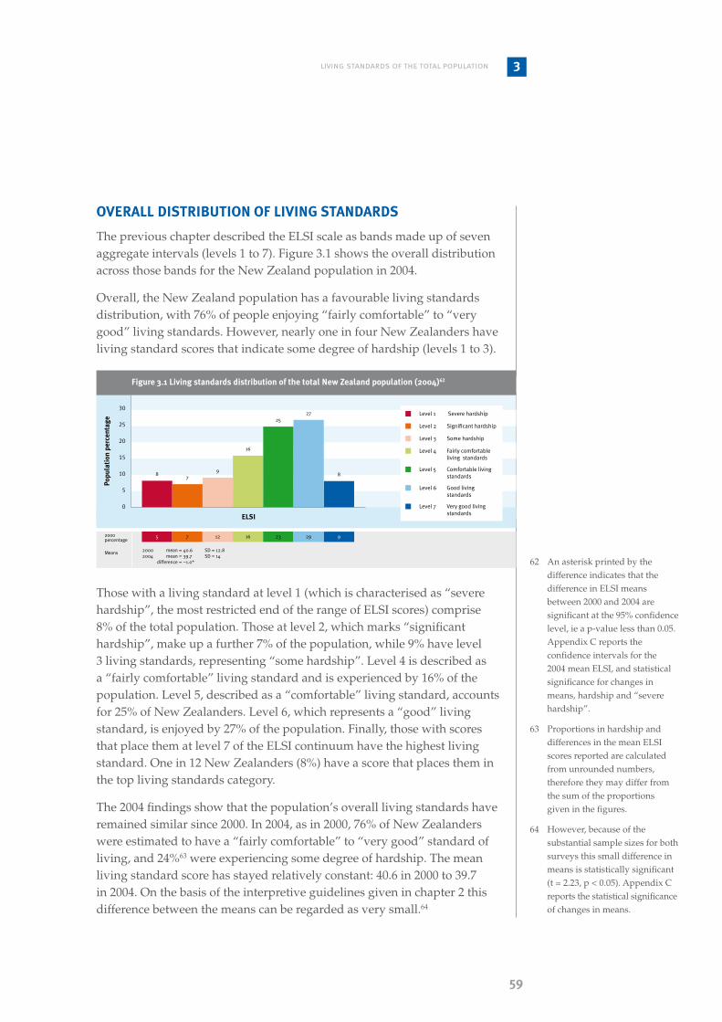
5�

living standards of the total population 3

overall distriBution of living standards

The previous chapter described the ELSI scale as bands made up of seven aggregate intervals (levels 1 to 7). Figure 3.1 shows the overall distribution across those bands for the New Zealand population in 2004.

Overall, the New Zealand population has a favourable living standards distribution, with 76% of people enjoying “fairly comfortable” to “very good” living standards. However, nearly one in four New Zealanders have living standard scores that indicate some degree of hardship (levels 1 to 3).

An asterisk printed by the difference indicates that the difference in ELSI means between 2000 and 2004 are significant at the 95% confidence level, ie a p-value less than 0.05. Appendix C reports the confidence intervals for the 2004 mean ELSI, and statistical significance for changes in means, hardship and “severe hardship”.

Proportions in hardship and differences in the mean ELSI scores reported are calculated from unrounded numbers, therefore they may differ from the sum of the proportions given in the figures.

However, because of the substantial sample sizes for both surveys this small difference in means is statistically significant (t = 2.23, p < 0.05). Appendix C reports the statistical significance of changes in means.

62�

63�

64�

ELSI

Popu

lati

on p

erce

ntag

e

5

30

25

20

15

10

5

0

Figure 3.1 Living standards distribution of the total New Zealand population (2004)62

87

27

16

9

25

8

Level 1 Severe hardship

Level 2 Significant hardship

Level 3 Some hardship

Level 4 Fairly comfortable living standards

Level 5 Comfortable living standards

Level 6 Good living standards

Level 7 Very good living standards

2000 mean = 40.6 SD = 12.82004 mean = 39.7 SD = 14 difference = –1.0*

5 7 12 16 23 29 9

Those with a living standard at level 1 (which is characterised as “severe hardship”, the most restricted end of the range of ELSI scores) comprise 8% of the total population. Those at level 2, which marks “significant hardship”, make up a further 7% of the population, while 9% have level 3 living standards, representing “some hardship”. Level 4 is described as a “fairly comfortable” living standard and is experienced by 16% of the population. Level 5, described as a “comfortable” living standard, accounts for 25% of New Zealanders. Level 6, which represents a “good” living standard, is enjoyed by 27% of the population. Finally, those with scores that place them at level 7 of the ELSI continuum have the highest living standard. One in 12 New Zealanders (8%) have a score that places them in the top living standards category.

The 2004 findings show that the population’s overall living standards have remained similar since 2000. In 2004, as in 2000, 76% of New Zealanders were estimated to have a “fairly comfortable” to “very good” standard of living, and 24%63 were experiencing some degree of hardship. The mean living standard score has stayed relatively constant: 40.6 in 2000 to 39.7 in 2004. On the basis of the interpretive guidelines given in chapter 2 this difference between the means can be regarded as very small.64

2000 percentage

Means

60

Although the average ELSI score is almost unchanged from 2000 to 2004, and the mode of the distribution remains at level 6, some change is evident in the lower part of the distribution. The change is not large but is worth examining further at this point because it is repeated, in varying degrees, in many of the distributions presented later in this report.

The first point to note is that the proportion of the population in the hardship range of the ELSI scale (ie levels 1 to 3) has not changed: it is 24% in both years.65 However, the distribution within the hardship range has moved downwards over the period. In 2000, the proportions of the population in levels 3, 2 and 1 formed a downward sequence, with the figures being 12%, 7% and 5%. (This is what is typically found in the tail of a roughly normal distribution.) However, in 2004 the proportion at level 3 was 3% lower than in 2004 (which generally would be expected to be accompanied by declines at levels 2 and 1 also), while the proportion at level 1 (“severe hardship”) was 3% higher66 (the proportion at level 2 remained unchanged). These rises and falls have the effect of changing the shape of the lower part of the distribution. The 3% rise at level 1, although not large, is statistically significant.67

Thus while there has been no rise in the prevalence of hardship, there has been an intensification in hardship amongst those within the hardship range (levels 1 to 3). As might be expected, this is reflected in a rise in the average deprivation score (DEPSCORE)68 of those within the hardship range. The DEPSCORES for the hardship group (levels 1 to 3) in 2000 and 2004 were 3.31 and 3.61, respectively, with the difference being statistically significant.69

This phenomenon, intensification in hardship without a rise in prevalence, is initially surprising. In general, it would be expected that any economic changes that would produce a rise in “severe hardship” would also produce a rise in hardship generally, with a thickening of the whole of the lower part of the distribution. Extensive exploratory analysis was therefore carried out to gain some understanding of the observed changes. The results indicated that the complex change at the population level arises from different patterns of change having occurred amongst certain sub-populations. The population results show the combined effect of those different patterns of change.

Refer to appendix C for the statistical significance of changes in hardship.

Refer to appendix C for the statistical significance of changes in “severe hardship”.

A p-value less than 0.001.

The composition and properties of the DEPSCORE are described in chapter 2.

It is important to keep in mind that the results for 2000 and 2004 are from two independent cross-sectional surveys, not from a single longitudinal study in which the same group of people were each interviewed on two occasions, four years apart. Thus when it is said, for example, that beneficiaries with children showed a rise in the proportion in severe hardship, this is a short-hand way of saying that the proportion for the 2004 group of beneficiaries with children was higher than the proportion for the corresponding group in 2000. It is not reporting a change for a particular set of individuals.

65�

66�

67�

68�

69�

61


The group contributing most strongly to the change is that comprising beneficiary families with children. Although results for that group are fully reported later, it is helpful, in this chapter, to bring forward some of those results that are most salient to understanding the change in the lower part of the population distribution.70

In 2000, beneficiaries with children had very depressed living standards and presented a distribution that was quite distinct from the rest of the population. In particular, the mode was at level 3 (which is part of the hardship range), with two-thirds (68%) of the group at that level or lower.71 For the rest of the population, the mode was at level 6. There was a strong downward movement in the already-depressed ELSI distribution between the beneficiaries with children group in 2000 and the corresponding group in 2004. The mode dropped from level 3 to level 1, with the proportion at level 3 reducing by half (from 26% in 2000 to 13% in 2004) and the proportion at level 1 increasing by a comparable amount (from 21% to 34%). For the rest of the population, by contrast, the ELSI distribution showed little change. The effect on the population distribution was to reduce the overall proportion at level 3, leave unaltered the proportion at level 2 and increase the proportion at level 1.

The changes for beneficiaries with children are reflected more strongly in the results for some sub-populations (eg people of Mäori ethnicity and children) than they are in the population as a whole. This will be highlighted where the results for such sub-populations are presented, throughout subsequent chapters of the report.72

In the next part of this chapter, results are given separately for a variety of social and demographic groups, following which results are given according to financial circumstances. The chapter ends with an examination between living standards and various common types of adversity.

The exploratory analysis pointed to changes in some other sub-populations that also contribute to the changes in the population distribution between 2000 and 2004, but their effects are smaller than those produced by the reduction in the living standards of beneficiaries with children.

The figures given in this discussion – as for all results in this chapter – relate to population estimates of numbers of individuals in the designated categories. Thus “beneficiaries with children” is a short-hand reference to all members of EFUs comprising beneficiaries with children.

The changes in the distribution for beneficiaries with children are not, of course, reflected in sub-populations (such as people whose main income is from market sources) that do not include any beneficiaries with children.

70�

71�

72�

62

Adult respondents aged 18 years and over are weighted to represent the total adult population. Children in this study were not surveyed in their own right but are counted in the EFUs of which they are members. As stated on page 9 the living standard score assigned to the relevant EFU is assigned to the child or children in the unit. The children in the sampled EFUs are weighted to represent the count of children in the total population.

73�

variations in living standards across demographic and social groups

Living standards vary across the population depending on a number of social and demographic factors. This section examines variation in living standards in relation to characteristics such as age, ethnicity, EFU type, region, housing tenure, education, occupation, and income source. There are three reasons for those considerations being selected.

There is a long-standing concern about equitable social outcomes and, in the interests of equity, a view that disadvantage should not be concentrated in particular social and demographic groups, eg age groups or ethnic groups.

There is special concern about the wellbeing of children. This concern stems from evidence that childhood hardship can have long-term negative consequences and that children cannot affect their own living standards (to any great extent).

Policies are increasingly targeted using risk characteristics (known to be predictive of hardship/deprivation). Therefore, there is interest in knowing how well various characteristics indicate risk of lower living standards.

Age�3

Living standards vary considerably by age. In broad terms, the results shown in figure 3.2 show a similar pattern to 2000 and indicate a rise in living standards as age increases.

•

•

•

63


Children’s living standards show a great deal of variation, with 26% of children in the bottom two levels of the ELSI scale and 23% in the top two levels.

Children have the lowest average living standard of all the age groups. They are disproportionately at the lower end of the ELSI scale, with more than one in three (38%) in some degree of hardship. This result mirrors findings from other research showing that, compared with adults, there is a higher rate of income poverty amongst children.75, 76 However, this group also has the feature of showing a great degree of variation in living standards, with 23% in the top two levels. The diversity in children’s scores is reflected in their having a higher standard deviation than any other age group.

What underlies this high variation? Chapter 4 will show that children in two-parent non-beneficiary families have predominantly “comfortable” or “good” living standards, with this group having an ELSI mean of 39.7, which is the same as for the overall population. By contrast, children in beneficiary families have a high prevalence of hardship (74%), with a very low mean ELSI score of 20.6. This high level of hardship in a segment of the child population gives cause for a continued policy focus on child poverty. This focus reflects the accumulation of a strong body of evidence demonstrating the detrimental implications of poverty for child development.

Refer to appendix B for the distributions within ELSI levels by differing social and demographic factors and the relative sizes of the groups as a whole. These are reported for all figures in chapter 3.

For example, Ballantyne et al. 2004.

Ballantyne et al. use 50% of the median equivalised household income as the measure.

74�

75�

76�

Dependent children under 18 years

Age group

Popu

lati

on p

erce

ntag

e

50

45

40

35

30

25

20

15

10

5

0

Figure 3.2 Living standards distribution of total population by age groups (2004)74

18–24 years 25–44 years 45–64 years 65 years and over

1412 12

17

22

18

53

6

13

22

30

22

4

87

10

18

27

24

75 5

7

11

23

35

14

1

34

11

27

44

10

2000 mean = 36.4 SD = 13.72004 mean = 34.4 SD = 15.5 difference = –1.9*

8 10 18 19 20 19 6


2 6 11 20 27 27 7

2000 mean = 39.9 SD = 12.62004 mean = 39.1 SD = 13.6 difference = –0.8

5 7 13 18 24 25 8

2000 mean = 43.2 SD = 12.62004 mean = 43.3 SD = 13.4 difference = 0.0

4 4 9 12 22 36 11


1 1 5 9 22 50 13

Severe hardship Significant Some hardship Fairly comfortable Comfortable Good living Very good hardship living standard living standard standard living standard

2000 percentage

Means

64

The overall living standard distribution for the 18–24-year-old group remains favourable, with more than half having living standard scores described as “comfortable”, “good” or “very good”. The favourable position of this group, despite the fact that many have low incomes, may reflect the fact that many 18–24 year olds live in multi-family households (ie with parents or flatmates77) and are able to draw on the living standards of others, either through shared resources or through economies of scale. Earlier analysis undertaken on 2000 survey data indicated that 18–24 year olds residing with their parents tended to have better living standards than those not residing with their parents.78 In support of this, Jensen et al. (2002) showed that sole-parent mothers under the age of 25 had a lower risk of being in hardship than those over age 25, particularly when they lived in multi-family households.

The mean living standard scores of New Zealanders aged 25–44 and 45–64 are 39.1 and 43.3 respectively. While there has been little change in the mean scores for these groups since 2000, figure 3.2 shows there has been some change in living standard distribution. The proportion of 45–64 year olds with living standard scores in the “very good” category has increased from 11% to 14%, now the highest proportion of any age group in this category.

New Zealanders aged 65 years and over have the most favourable living standard distribution of all age groups. They are over-represented in the higher living standards levels and under-represented in the categories denoting some degree of hardship. Between 2000 and 2004 there was little change in the mean living standards of this age group and similar proportions showed some degree of hardship (about 8%). The living standards of older New Zealanders and the factors contributing to the living standards of older New Zealanders is examined in more detail in chapter 5.

In 2004, as in 2000, the pattern of ELSI scores with respect to age shows dependent children to have a greater prevalence of hardship than other age groups, with child hardship strongly concentrated in benefit families. People aged 65 years and older are substantially less likely to be at the lower end of the range, while those aged 18–64 years are in an intermediate position. The estimated patterns of living standards across the age groups are consistent among ethnicities.

Interestingly, between 2000 and 2004 the proportion of 18–24 year olds who were residing away from parents/caregivers increased from 47% to 61%. Many of these young people are likely to be participating in education or training and therefore have limited incomes.

Ministry of Social Policy 2001.

77�

78�

65


Living standards by age and family composition

New Zealand Living Standards 200079 presented results obtained by applying a life-stage framework that postulates movement through a stylised sequence of living situations from youth to old age. Focusing on the life cycle phases that involve some degree of economic independence, the stages can be characterised as:

I young, financially independent, single adult, who acquires a partner to become part of a

II young couple without children, who have children, to become part of a

III couple with children, whose children grow up to leave home, at which stage they are a

IV middle-aged couple without children, who withdraw from the paid workforce, to become a

V retired couple, who are eventually reduced by bereavement, to a

VI retired single person.

It is sometimes postulated that the first two stages (involving at least modest incomes that are not required to be stretched for the support of dependent children) will give rise to adequate-to-good living standards, which can be expected to fall at the point where the couple have children, followed by a rise after the children have become independent, and then a decline following retirement. In table 3.1 the cells corresponding to this sequence are shown in bold. What the table suggests is that for those who follow this life course, living standards generally follow the pattern postulated until the older ages, where living standards continue to be high (on average) rather than showing a decline. Table 3.1 also signals the many different trajectories that may be followed over the life course, suggesting that different trajectories may give rise to varying patterns of rise and fall. The 2004 pattern of living standard means by EFU type and age is similar to that for 2000.

It is necessary to be cautious about interpreting cell values as indicating the likely pattern of changes that will occur for individuals over the course of their lives, because the sequence of social and economic conditions encountered at various ages is likely to be different for each generational cohort. Thus, for example, the relatively favourable living standards of the current set of people aged 75 years and older may not represent the situation of people who reach that age in 20 years’ time.


79�

66

Gender

The ELSI scale is primarily a measure for the EFU, which means that the score distributions for partnered males and females will essentially be the same, with the exception of small differences associated with sampling and the effects of gender-related responses. For this reason, the results presented here are just for single adults as well as for the adult population as a whole.

Figure 3.3 shows that there is a higher proportion of single females in hardship (30%) than single males in hardship (19%). Similarly, the mean living standard scores for these two groups show lower living standards for females (37.7) compared to males (40.2). Between 2000 and 2004 however, there has been an increase in hardship for both single men and women.

Table 3.1 Average living standard scores of population aged 1� years and over by age and family composition of the respondent (2004)80

EFU type 1�–24 years

25–2� years

30–34 years

35–54 years

55–64 years

65–�4 years

�5 years plus

Single without children 40.1 41.6 39.4 38.1 39.0 41.9 4�.4

Couple without children 39.7 42.4 45.8 46.7 4�.� 46.0 47.8

Couple with children 35.2 36.5 3�.5 40.4 41.3 – –

Single with children 28.1 27.6 24.6 27.8 – – –

Bold cells indicate typical progression through the life-cycle model.

80�

Female

Gender of single person/sole parent

Popu

lati

on p

erce

ntag

e

35

30

25

20

15

10

5

0

Figure 3.3 Living standards distribution of single people aged 1� years and over by gender (2004)

98

13

17

2425

56 6

7

19

29

26

7

Male


6 7 13 17 23 29 6 2 5 10 16 26 31 9



2000 percentage

Means

6�


Figure 3.3 shows that on average single men have moderately higher living standards than single women. This can be further examined by distinguishing between those with and without dependent children. Table 3.2 shows that living standards between genders are virtually the same for single people without dependent children living with them (40.9 for males and 40.5 for females). Average living standards are slightly lower for females with dependent children at 26.8 compared to 29.6 for single males with dependent children. The major difference in living standards for single people between genders arises due to a higher proportion of single females having dependent children than single males (20% compared to 6%). As a consequence more females are in receipt of the Domestic Purposes Benefit than males.

Table 3.2 Average living standards of single people aged 1� years and over by gender and dependent children (2004)

Single without children Single with children All single

Male 40.9 29.6 40.2

Female 40.5 26.8 37.7

Female

Gender of total adult population

Popu

lati

on p

erce

ntag

e

35

30

25

20

15

10

5

0

Figure 3.4 Living standards distribution of total population aged 1� years and over by gender (2004)

6 6

9

15

25

30

9

45

7

16

27

31

10

Male


4 6 11 16 23 32 9 3 5 10 15 24 33 10


Figure 3.4 shows a roughly similar distribution of living standards and similar average living standard scores for all males and females aged 18 years and over. This is related to the fact that male–female couples living together as a family unit are assumed to have equal living standards. The higher levels of hardship for females (21%) compared to males (17%) can be accounted for by those females who are single or sole parents, as shown in figure 3.3.


2000 percentage

Means

6�

Ethnicity81

The following results provide a brief overview of the living standards and changes in living standards since 2000 of Mäori, Pacific, European and other82 ethnic groups.

Ethnic categories are not mutually exclusive; ethnicity is based on total responses to the ethnicity question. For example, if an adult respondent, or their partner or child, specified Pacific as one of their ethnicities, they are all counted as part of the Pacific ethnic group. This procedure is followed for all the ethnic groups. Note that this definition differs from that used in chapter 4, which assigns an ethnicity classification to the EFU.

All ethnic groups not listed above are grouped in the “other” category. This is because these groups are not large enough to constitute a category for analysis on their own.


Due to the groups not being mutually exclusive, the proportions do not add up to 100%.

Both of these increases in the severe hardship category are statistically significant with a p-value less than 0.001 for Mäori and 0.002 for Pacific people.

81�

82�

83�

84�

85�

Mäori

Ethnicity

Popu

lati

on p

erce

ntag

e

35

30

25

20

15

10

5

0

Figure 3.5 Living standards distribution by ethnicity (2004)83

Pacific European

17

1112

17

25

15

3

27

15 15

9

14

19

1

25

46

15

26

30

910

Other

9 9

56

28

19

2000 mean = 34.5 SD = 12.4 2004 mean = 32.8 SD = 15.3 difference = –1.6

7 11 23 21 23 11 4



15 17 24 17 15 10 1 3 5 9 15 24 34 11


6 7 16 21 21 25 0

The distribution of living standards by ethnicity reveals marked differences for the groups. Figure 3.5 shows that ELSI scores are bunched towards the lower end of the living standard scale for Mäori and Pacific populations and are tending towards the top of the scale for Europeans. It is important to consider the different sizes of the groups. Using the 2004 living standards survey data to estimate population proportions, around 75% are European, 15% are Mäori, 10% are Pacific and 10% are classed as other.84

Forty percent of Mäori and 58% of the Pacific population were in some degree of hardship, compared to only 19% of Europeans. In contrast, the majority of Europeans (66%) and others (58%) have living standards that are described as “comfortable”, “good” or “very good”.

While there has been almost no change in the proportions of the Mäori and Pacific populations experiencing some degree of hardship, among those experiencing hardship more were skewed towards the “severe hardship” end of the living standards continuum. For example, in 2000, 7% of Mäori and 15% of Pacific people were in “severe hardship”. By 2004 this had increased to 17% and 27% respectively.85


2000 percentage

Means

6�


Table 3.3 Living standards of the New Zealand Pacific population aged 1� years and over by country of birth (2004)

Mean ELSI % in hardship

Born in New Zealand 32.5 38

Born elsewhere 28.1 57

The lower living standards of Pacific people born outside of New Zealand may reflect the costs of immigration and resettlement, adaptation difficulties and discrimination, and possibly the fact that this group makes higher transfers to relatives who are living overseas. A further, more comprehensive study of living standards has been designed to more specifically examine the factors contributing to the variation in Pacific living standards and the uniqueness of this population in New Zealand.

Breakdowns by country of birth are not given for other ethnic groups because the respondent numbers are insufficient to give informative results.

In 2000, there was a difference of 13.1 points between the means for the Pacific and European populations. In 2004, the difference in means had increased slightly to 15.7, suggesting a small increase in disparity between the living standards of these ethnic groups. Amongst the Pacific population, there has been an increase in the proportion reliant on income-tested benefits from 22% in 2000 to 26% in 2004. Mäori have significantly more reliance on income-tested benefits than Europeans, although to a lesser degree than Pacific people. Analysis later in this chapter will show how the population (especially those with dependent children) reliant on income-tested benefits have had a significant fall in their living standards over this period.

The 2004 survey contained a question (that was not in the 2000 survey) on country of birth. The question was included partly in response to suggestions to the effect that Pacific people born in New Zealand are likely to be better established on average than those born elsewhere and consequently are likely to have better living standards. Comparisons between these two subgroups are given in table 3.3, which shows those born in New Zealand having a mean standard of living which is 4.4 points greater than that of those born elsewhere (32.5 and 28.1 points respectively). In addition, a greater proportion of those who were born overseas are in some level of hardship (57% compared with 38%).

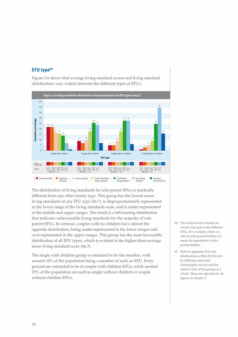
�0

EFU type86

Figure 3.6 shows that average living standard scores and living standard distributions vary widely between the different types of EFUs.

The analysis here is based on counts of people in the different EFUs. For example, where we refer to sole-parent families we mean the population in sole-parent families.


86�

87�

Single with children

EFU type

Popu

lati

on p

erce

ntag

e

45

40

35

30

25

20

15

10

5

0

Figure 3.6 Living standards distribution of total population by EFU type (2004)87

Couple with children Single without children Couple without children

22 22

1716

14

7

1

53

56

16

1

40

9

5

18

28

25

28

997

10

2426

18

7

4 8 14 18 24 24 8 2 3 7 11 23 41 133 5 10 16 25 33 817 14 26 21 13 7 1





The distribution of living standards for sole-parent EFUs is markedly different from any other family type. This group has the lowest mean living standards of any EFU type (26.7), is disproportionately represented in the lower range of the living standards scale, and is under-represented at the middle and upper ranges. The result is a left-leaning distribution that indicates unfavourable living standards for the majority of sole-parent EFUs. In contrast, couples with no children have almost the opposite distribution, being under-represented in the lower ranges and over-represented in the upper ranges. This group has the most favourable distribution of all EFU types, which is evident in the higher-than-average mean living standard score (46.3).

The single with children group is estimated to be the smallest, with around 10% of the population being a member of such an EFU. Forty percent are estimated to be in couple with children EFUs, while around 25% of the population are each in single without children or couple without children EFUs.


2000 percentage

Means

�1


In 2004, there is a difference of 19.6 points between the mean living standard scores of sole-parent families and couples with no children. This difference has increased from 16.7 points in 2000, indicating a small increase in disparity between EFU types.

There has been very little change since 2000 in the proportion of sole-parent EFUs in levels 5, 6 and 7, indicating the downward shift has occurred primarily from the middle to lower end of the scale. Couples with children show a similar pattern of change although not quite as pronounced as sole-parent EFUs. In contrast, the distribution for single-person EFUs has moved from the higher levels towards the middle and the distribution of couple-only EFUs has shifted from the middle levels upward.

Region

The current survey classifies New Zealand into five regional areas: Auckland, Wellington, other major urban areas, secondary and minor urban areas, and rural New Zealand. As geographical areas differ in levels of employment, incomes and other socio-economic indicators, corresponding differences in living standards could be expected. However, the broad breakdown used here limits the extent to which that issue can be examined. Figure 3.7 shows that in 2004 there is relatively little difference between mean living standard scores by region.88

The Auckland and Wellington areas presented here are based on the Auckland and Wellington Regional Council areas.

88�

Auckland

Region

Popu

lati

on p

erce

ntag

e

35

30

25

20

15

10

5

0

Figure 3.� Living standards distribution of total population by region (2004)

Wellington Other major urban areas

Secondary and minor urban areas

Rural New Zealand

108

10

16

21

25

10

6

910

15

23

28

9

67 9

16

28 28

7 7 79

14

28 28

7 75

9

17

24

29

8


5 8 16 17 21 25 8


3 5 9 20 20 31 12


5 7 11 16 24 28 9


4 6 12 16 23 33 7


4 5 10 13 26 32 10


2000 percentage

Means

�2

People living in Auckland have the lowest mean living standard score of all regions (38.3) and the highest proportion with ELSI scores indicating some degree of hardship (28%). People in rural New Zealand and other major urban areas have the highest mean ELSI scores (40.8% and 40.3%) and are the least likely to be in hardship (21% each).

People living in Wellington have had an increase in the proportion of the population experiencing some degree of hardship (from 17% in 2000 to 25% in 2004). The pattern of change for the Auckland population is somewhat different, with increases at both the highest and lowest ELSI levels, which may suggest increasing inequality for people in this region.

Housing tenure

Figure 3.8 shows the very different living standards distributions of EFUs based on housing tenure. Homeowners, with and without mortgages, have right-leaning distributions, indicating favourable living standards, while Housing New Zealand (HNZC) tenants have a left-leaning distribution.

Refer to appendix B for the distributions within ELSI levels by differing social and demographic factors and the relative sizes of the groups as a whole. These are reported sfor all figures in chapter 3.

89�

Rented – HNZC

Housing tenure

Popu

lati

on p

erce

ntag

e

60

55

50

45

40

35

30

25

20

15

10

5

0

Rented – private landlord

Local authority Owned with mortgage

39

1617

12

24

12

54

86

14

28

31

99

26

43

15

68

18

2729

87

11

18

54

6

2

11

15

19

24

15

4

15

8

4

0

Owned mortgage free

Figure 3.� Living standards distribution of total population by housing tenure (2004)89

Family trust


20 28 24 13 11 5 0 2 5 10 15 25 30 121 1 5 9 22 45 164 4 11 17 25 31 87 12 28 9 22 22 18 11 18 22 21 16 2







2000 percentage

Means

�3


The mean living standards of mortgage-free homeowners are the highest of any housing tenure group (47.1). The mean for family trusts and mortgaged homeowners are considerably lower (41.8 and 41.6 respectively), but still indicate very high average living standards relative to other groups.

Living standards are lowest among HNZC tenants, with those in 2004 having lower mean living standards (21.6) than HNZC tenants in 2000 (25.4). Thirty-nine percent of HNZC tenants in 2004 have living standard scores in the lowest ELSI interval, compared to 20% in 2000. HNZC tenants are at least three times more likely than any other group to be in “severe hardship”. The main reason why this group has markedly lower living standards is that HNZC housing is allocated on the basis of need. Government policy on rental charges for HNZC properties changed from market-related rents to income-related rents between the two surveys, with a consequential tightening of the targeting of state housing to those in hardship. As at June 2004, around half (53%90) of HNZC’s tenants had also been HNZC tenants at June 2000. This indicates that there has been a large shift in the composition of tenants, with those housed after 2000 being selected from waiting lists using a social allocation criterion. It must also be noted that those renting from HNZC are a small group comprising around an estimated 5% of the population.

The income-related rents policy has the effect of providing most tenants with a higher level of rent subsidy than they would otherwise have been receiving,91 thus reducing the financial pressures on those families. However, it is clear that many of them continue to be in considerable hardship. The very low mean score for the 2004 tenants almost certainly is the outcome of a more targeted selection process that favours those who have multiple sources of deprivation.

With regard to local authority tenancies, allocation policies vary. The pattern of living standards for people who rent from local authorities has shifted towards the centre of the ELSI scale.92 In 2004, 54% of this group have living standard scores at level 5 (described as “good”) compared to 22% in 2000, and only 20% were in some degree of hardship (levels 1, 2 and 3), down from 47% in 2000. This may reflect changes in the numbers and/or allocation of local authority-owned housing.

Housing New Zealand 2005.

In June 2000 the mean HNZC rent was $165 per week. In June 2004 the mean HNZC rent for those paying an income-related rent was $88 per week. For those paying market rent the mean was $198 per week (Housing New Zealand 2005).

These findings are based on a small sample size and may not be representative of local authority tenants as a whole.

90�

91�

92�

�4

Although homeownership seems to be an indicator of superior living standards, the rate of homeownership has been falling in recent years and is indeed predicted to continue to fall into the future.93 As at June 2004 home affordability, as measured by AMP’s National Home Affordability Index, had fallen for eight consecutive quarters.94 Although wages continued to rise, the increase in median house prices far exceeded them. This highlights the increasing difficulty first-home buyers are encountering getting their feet on the first rung of the ownership ladder. The Government’s 2005 Budget included measures intended to ameliorate this difficulty.95

Education

Figure 3.9 presents the living standard distribution for four levels of educational qualification (no formal qualification, school qualification, occupational certificate or diploma, and Bachelors degree or higher) and the change in distribution since 2000. It shows that overall there is a positive association between living standards and levels of qualifications obtained.

DTZ Research 2004.

Crews 2004.

The 2005 Government Budget included measures designed to help people develop a long-term savings habit and toward the purchase of their first home. The package has three components: • Kiwi Saver is a voluntary work-based savings scheme designed to utilise the existing PAYE (pay as you earn) tax system. Kiwi Saver includes a first home deposit subsidy (of up to $5,000) • a substantial expansion of the Mortgage Insurance Scheme • education programmes to improve financial literacy for first-home buyers.

93�

94�

95�

No formal qualification

Highest educational qualification

Popu

lati

on p

erce

ntag

e

40

35

30

25

20

15

10

5

0

Figure 3.� Living standards distribution of population aged 1� years and over by highest educational qualifications (2004)

School qualification Occupational certificate or diploma

Bachelors degree or higher qualification


6 7 13 17 23 29 6

12

89

1820

30

4


4 6 9 15 23 36 8


3 5 12 15 26 31 9


2 2 7 14 21 36 19

5 5

9

26

29

16

9

56

13

28

23

30

9

45

8

15

2

36

15


2000 percentage

Means

�5


People with no formal qualifications are the most likely to have living standard scores at the lower end of the ELSI distribution (levels 1–3). Twenty-nine percent of people in this group were in hardship, compared to 11% of people with a Bachelors degree or higher. The high representation of people with no formal qualification at level 6, described as having “good” living standards, may in part be a consequence of the favourable living standard distribution of older New Zealanders, who tend to have lower levels of formal education. The living standards of older New Zealanders are explored in more detail in chapter 5.

Since 2000, there has been an increase in “severe hardship” amongst those with no formal qualifications and their average living standards score has fallen slightly from 39.6 in 2000 to 37.3 in 2004. In 2004, those with no formal qualifications continued to have an average living standard score which was below that of the overall population.

Standardising for age – controlling for the effect of older people predominantly found in the lower education group – strengthens the relationship between mean living standards and education (see table 3.4).

Occupation

Figure 3.10 shows the ELSI distribution for various major occupational groups based on the New Zealand Standard Classification of Occupations (NZSCO90). The occupational groups are ranked from highest to lowest on the basis of skill requirements to perform a job.96 The analysis is based on the working-age population (18–64 years) who are in single-earner EFUs and are in full-time employment. This enables a more focused examination of the association between occupation and living standards without the confounding influence of variation in hours worked and multiple-earner EFUs.

Table 3.4 Mean ELSI score and mean score standardised for age by highest educational qualification of those aged 1� years and over (2004)

Qualification ELSI mean Age-standardised mean

No formal qualification 37.3 35.1

School qualification 41.0 41.2

Occupational certificate or diploma 41.4 41.2

Bachelors degree or higher qualification 45.2 45.7

It has been common practice to rank the agriculture and fisheries occupational sector just above trade, plant and machinery workers when presenting this type of data (Statistics New Zealand 1998a). However, the agriculture and fisheries group is very mixed, containing farmers and agricultural contractors with substantial incomes along with farm labourers and unskilled agricultural workers. In this analysis, as in the 2000 report, the agricultural group is placed above clerical, service and sales workers. This is because their overall living standard resembles those of the “higher-skilled” occupations rather than those of the “lower-skilled” occupations.

96�

�6

Among the full-time employed population aged 18–64 years who are in single-earner EFUs, those with elementary occupations (ie “lower-skilled” occupations) have the lowest mean living standards score (38.1); legislators, administrators and managers have the highest mean living standards score (45.7) and all other occupational groups fall between these scores. On average, living standards have fallen for elementary and professional workers.

Figure 3.10 shows that the majority of full-time employed, working-age people are located in the upper three living standards intervals, regardless of occupation. The two occupational groups with the highest mean scores, legislators, administrators and managers and professionals, have right-leaning distributions, with a clear majority of these populations having “comfortable” to “very good” living standards.

The living standards of the self-employed

Among the population receiving market income, information was collected on whether they received income from self-employment earnings or wages and salaries. It is estimated that around 15% of those receiving a market income were self-employed.

EFUs with income primarily from self-employment have equivalent disposable incomes that are a little higher than those whose income is primarily from wages and salaries. On this basis it might be expected that

Elementary occupations

Major occupational groups

Popu

lati

on p

erce

ntag

e

45

40

35

30

25

20

15

10

5

0

Trades, plant and machinery

Clerks, service and sales

Professionals


2 2 13 15 29 35 5

11

35

21

5 6 16 19 27 20 6



5

98

32

1

6

14

25

17

78

14

23

10

7

13 13

2628

0 3 6 11 28 34 180 3 0 15 20 41 142 5 15 17 26 29 6

6

12

15

32

21

5

19

1

Legislators, administrators and managers



Figure 3.10 Living standards distribution of population aged 1�–64 years in EFUs with a single income earner who is full-time employed by occupational groups (2004)

40

35 35


2000 percentage

Means

��


the former group would have higher living standards than the latter. In addition, it can be speculated that some self-employed people may be better off than income data alone suggests, because they are able to boost their consumption (and thus their living standards) at the expense of their declared income. Some support for this idea was provided by exploratory regression analyses (referred to in chapter 2) that gave estimates of ELSI scores on the basis of income, assets and some other explanatory variables. The results indicated that people with income from self-employment had average ELSI scores that were higher than would be expected from the explanatory variables, suggesting that there may be some feature of self-employment, distinct from the reported level of income it provides, that independently elevates living standards.

Figure 3.11 examines the living standards distributions of those aged 18–64 years who are full-time employed and are members of single-earner EFUs. As mentioned earlier, this segmentation of the population enables a more focused examination of the association between market income source and living standards without the confounding influences of variation in hours worked, multiple-earner EFUs, and variation in sources of income for those multiple-earner EFUs.

Self-employed

Income source of those with market incomes

Popu

lati

on p

erce

ntag

e

40

35

30

25

20

15

10

5

0

Figure 3.11 Living standards distribution of population aged 1�–64 years who are full-time earners in single-earner EFUs by market income source (2004)

21

3

14

3834

8

57

11

15

2628

8

Wages and salary

3834


1 2 10 17 24 35 11 3 5 12 16 26 30 9



2000 percentage

Means

��

Between 2000 and 2004 there was a decrease in self-employed people experiencing hardship to some degree (down from 13% in 2000 to 6% in 2004) and an increase in those with “comfortable” to “good” living standards (up from 70% in 2000 to 80% in 2004). The self-employed continue to have higher average living standards compared with wage and salary earners and the gap in mean living standards between these groups has increased from 2.3 to 5.1. This divergence may reflect the combined effect of several factors relating to the recent positive economic conditions. Improvements in employment prospects may have caused some marginal self-employed to move into wage and salary jobs. Those remaining in the self-employed group would tend to be those in a better position to take advantage of the strong economy. This is demonstrated by the fact that equivalent disposable income for wage and salary earners has only increased by one-fifth of that of the self-employed.

Income source

People reliant on income-tested benefits have low incomes and also a relatively high likelihood of other forms of disadvantage (sickness, disability, poor English language skills, etc). As a consequence, there has been a long-standing concern about their wellbeing by social policy makers and the public at large. Government policy has sought to find a socially acceptable balance between reducing hardship among beneficiaries and avoiding the creation of disincentives to self-reliance (and consequent poverty traps).

The following analysis divides the population into three mutually exclusive groups.97

Income-tested benefit specified here as people in EFUs where there was receipt of an income-tested benefit (core benefit) in the last 12 months and no one was in full-time employment at the time of the survey (this group comprised around 15% of the population).

New Zealand Superannuation specified here as people in EFUs where there was receipt of New Zealand Superannuation98 (this group comprised around 15% of the population).

Market income specified here as people in EFUs in neither of the above two categories and therefore receiving income primarily from market sources (this is by far the largest group, comprising an estimated 70% of the population).

•

•

•

Income source is defined using a prioritised classification. Some of the population here may have been in receipt of an income-tested benefit at some time during the past 12 months but were employed full-time at the time of the survey. Similarly, some superannuation recipients may have received an income-tested benefit before qualifying for superannuation during the year. Some in the income-tested benefits group may also have received income from market sources during the year but were not in full-time employment at the time of the survey. There is a 96% overlap between the main income source of EFUs and the prioritised definition of income source used.

The population in receipt of New Zealand Superannuation and those aged 65 years and older are not exactly the same. This is because on the one hand a small proportion of those over 65 years do not qualify for New Zealand Superannuation. On the other hand, some superannuitants have spouses aged under 65 years who are covered as non-qualifying spouses. The latter are more numerous than the former. Overall, the total number of people covered by New Zealand Superannuation is 9% greater than the total number of people aged 65 and older.

97�

98�

��


The distribution of the beneficiary group is very different from the distributions of the market income group and New Zealand Superannuitants. The latter two groups have strongly right-leaning distributions, with the peak frequency at level 6 (“good” living standards). For both groups, the mean ELSI scores (41.7 and 46.2 respectively) are higher than the mean for the overall population (39.7).

By contrast, the beneficiary group has a strongly left-leaning distribution in which the peak is at level 1 (“severe hardship”). The mean ELSI score is 25.6, which is more than a whole standard deviation below the population mean. This indicates that in 2004 the beneficiary group had very depressed living standards compared with New Zealanders as a whole.

This point is reinforced by examining the proportions at the hardship levels (ie levels 1 to 3). Sixty-one percent of the beneficiary group are in some degree of hardship, compared to 19% of the market income group and 8% of the superannuitants. The living standards distribution of beneficiaries within the lower categories is now bunched more strongly towards the lowest ELSI level, resulting in 26% being in “severe hardship” compared to 17% in 2000.

Income source

Popu

lati

on p

erce

ntag

e

50

45

40

35

30

25

20

15

10

5

0

Figure 3.12 Living standards distribution of total population by income source of EFU (2004)

Market income New Zealand Superannuation

4 5

9

16

2729

10

Income-tested benefits

26

21

14

19

16

4

01

34

10

27

10

45


3 5 11 16 25 31 10


17 18 22 21 16 6 1


1 1 5 9 21 50 12


2000 percentage

Means

�0

The question arises as to why the beneficiary group (unlike the market income and superannuation groups) has shown a substantial rise in “severe hardship” and reduction in the ELSI mean. Results given in New Zealand Living Standards 200099 showed that beneficiaries were a not a uniform group with respect to living standards, but that beneficiaries with children had substantially lower living standards than beneficiaries without children. It is of interest to examine whether this difference remains or has changed since the earlier survey. In addition, as noted in chapter 1, there have been changes in the numbers of people receiving different types of income-tested benefits, resulting in an overall reduction in the size and composition of the beneficiary group. It is also of interest, therefore, to examine whether these changes have altered the proportions of beneficiaries with and without children, thereby affecting the living standard distribution of the beneficiary group. These issues are considered below.

Figure 3.13 compares the living standard distributions of beneficiary EFUs with and without children. In broad terms, the 2004 distributions show the same sharp contrast as was found in 2000. Beneficiaries without children have a right-leaning distribution, with a peak at level 5 (“comfortable” living standard), while the beneficiaries with children have a left-leaning distribution, with a peak at the lowest living standard level (“severe hardship”).


99�

No children

Beneficiary EFUs with and without dependent children

Popu

lati

on p

erce

ntag

e

40

35

30

25

20

15

10

5

0

Figure 3.13 Living standards distribution of beneficiary EFUs by presence of children (2004)

14

11

15

22

3834

0

27

13

16

8

20

Have children


10 13 15 23 27 9 2 21 21 26 20 9 3 0


29

9

34


2000 percentage

Means

�1


The contrast between the shapes of the two distributions shown in figure 3.13 is reflected in the large difference between their ELSI means: 32.5 for beneficiaries without children compared with the much lower value of 21.1 for beneficiaries with children. Furthermore when these results are compared with the corresponding figures for 2000, it is found that the gap between the two beneficiary groups widened.

Beneficiaries without children have very similar distributions in the two survey years.100 The widening gap between beneficiaries with children and beneficiaries without children is the consequence of a moderate downward movement in the ELSI distribution for beneficiaries with children.101 In 2000 the peak of the distribution was at level 3, but by 2004 (as noted above) the peak was at level 1. This sharp downward movement resulted in a large increase in the proportion of beneficiaries with children who are in severe hardship, from 21% in 2000 to 34% in 2004.

Reference was made earlier to the possible contribution of changes in beneficiary numbers. In June 2000 the number of EFUs reliant on Unemployment Benefit was 146,000102 (of which 18% were EFUs with children). By 2004 this had reduced to 74,000 (of which 14% were EFUs with children). The corresponding numbers for Sickness and Invalid’s Benefits were 88,000 and 116,000 (14% with children in both years). For the Domestic Purposes Benefit there were 109,000 (96% with children) in 2000 and 110,000 (95% with children) in 2004.103 These changes in the numbers of EFUs receiving the various types of benefits resulted in a change in the composition of the overall beneficiary group. In 2000 Domestic Purposes Beneficiaries comprised 29% of the overall beneficiary group, with Unemployment Beneficiaries and Sickness and Invalid’s Beneficiaries comprising 63%. The corresponding figures for 2004 were 33% (Domestic Purposes Benefit) and 58% (Unemployment, Sickness and Invalid’s Benefits).

In relation to the earlier breakdown in figure 3.12, beneficiaries with children made up 41% of the beneficiary group in 2000 and 43% in 2004; that is to say, there has been a small rise in the proportion of beneficiaries who have children.

It is possible to estimate the reduction that would have occurred in the ELSI mean for the overall beneficiary group if there had been no change to the 2000 living standard distributions of those with children or those without children but a rise (as observed) in the proportion of beneficiaries who have children. This procedure shows the effect of the with/without-children compositional change from 2000 to 2004, without the effect of the change in

Beneficiaries without children are composed mainly of people receiving Unemployment Benefit and people receiving Sickness or Invalid’s Benefit. These two sets of beneficiaries have similar living standard distributions, with means of 33.8 and 32.3 respectively in 2000, and 31.7 and 30.9 in 2004. These means are in contrast to the much lower means for beneficiaries with children (see figure 3.13).

Beneficiaries with children are composed primarily of sole parents receiving Domestic Purposes Benefit. The remainder are almost all two-parent families receiving Unemployment Benefit or Sickness or Invalid’s Benefit. These different sets of beneficiaries with children have living standard means that are all substantially below the means of beneficiaries without children, and are all lower in 2004 than 2000. Figure 4.4, in chapter 4, gives the living standard distributions and means (for 2000 and 2004) of sole-parent beneficiaries with children and two-parent beneficiaries with children.

The beneficiary numbers in this section were obtained from MSD administrative data.

There were 28,000 (40% with children) receiving other types of benefits in 2000 and 27,000 (42% with children) in 2004, a fall of 1,000.

100�

101�

102�

103�

�2

the living standard distributions. It is found that this compositional change, by itself, would have caused the ELSI mean for the beneficiary group to drop by 0.2 of an ELSI point, which is less than one-tenth of the drop that has occurred.

In a similar way, it is possible to estimate the reduction that would have occurred in the ELSI mean for the beneficiary group if there had been changes (as observed) in the living standard distributions of the constituent subgroups but no compositional change. Specifically, the result shows how much of the reduction was due to the living standards drop for beneficiaries without children (which was small) and the drop for beneficiaries with children (which was much larger). It is found that the drops for those subgroups account for nine-tenths of the reduction that occurred in the ELSI mean of the beneficiary group.104

The conclusion that can be drawn from these results is that the drop in the living standards of the beneficiary group is not (to any great extent) a consequence of the compositional change in the group but is primarily the consequence of the reduced living standards (and large rise in “severe hardship”) of those beneficiaries who have children. The reasons for this are not known. They may include increased pressures on parents to meet rising education-related and health costs and the costs of managing increased levels of personal debt. Another factor could be that there was a slight decrease in the benefit income received by Domestic Purposes Beneficiaries (the largest group of beneficiaries with dependent children), largely due to the non-indexation of Family Support. However, these speculations cannot be tested within the context of the study because the information that would be required for that analysis was not collected in the surveys.

A small amount of the reduction (less than one-twentieth) is due to an interaction between the compositional change and the living standards changes within the constituent subgroups.

104�

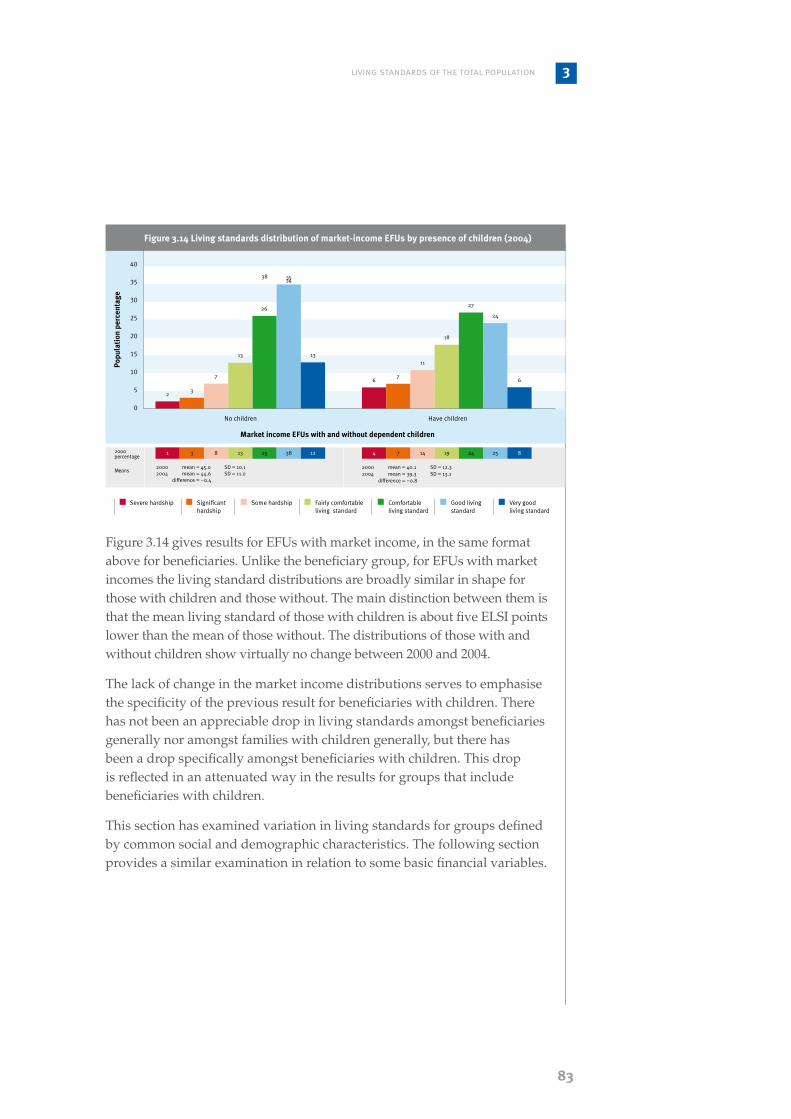
�3


No children

Market income EFUs with and without dependent children

Popu

lati

on p

erce

ntag

e

40

35

30

25

20

15

10

5

0

Figure 3.14 Living standards distribution of market-income EFUs by presence of children (2004)

23

7

13

3834

13

7

11

18

27

24

Have children


1 3 8 13 25 38 12 4 7 14 19 24 25 8


26

35

6 6

Figure 3.14 gives results for EFUs with market income, in the same format above for beneficiaries. Unlike the beneficiary group, for EFUs with market incomes the living standard distributions are broadly similar in shape for those with children and those without. The main distinction between them is that the mean living standard of those with children is about five ELSI points lower than the mean of those without. The distributions of those with and without children show virtually no change between 2000 and 2004.

The lack of change in the market income distributions serves to emphasise the specificity of the previous result for beneficiaries with children. There has not been an appreciable drop in living standards amongst beneficiaries generally nor amongst families with children generally, but there has been a drop specifically amongst beneficiaries with children. This drop is reflected in an attenuated way in the results for groups that include beneficiaries with children.

This section has examined variation in living standards for groups defined by common social and demographic characteristics. The following section provides a similar examination in relation to some basic financial variables.


2000 percentage

Means

�4

living standards By financial characteristics of the population

Previous research105 has indicated that people’s living standards reflect the combined effects of many factors, some relating to their current circumstances (eg current income, housing costs) and some relating to life history (eg death of a partner in the preceding decade, marital separation involving property settlement, business failure, being the victim of crime). This section examines the way in which living standards vary with income, asset position and housing costs. Results on the relationship between living standards and some indicators of adversity are presented in part 4.

Income106

The analysis in figure 3.15 is based on the annual income for the EFU. The income variable ranks the population in EFUs by their equivalent disposable incomes. The equivalisation procedure is used to account for variations in family size and composition.107 In 2004 living standards increased consistently with disposable income.

Fergusson et al. 2001.

The income data used here for 2000 has been Consumer Price Index-adjusted to the 2004 base year.

The income of the EFU has been adjusted using the 1988 Revised Jensen Equivalence Scale (RJS). The RJS is a set of ratios (calculated to allow for economies of scale and the differential consumption by adults and children) that specify the relative incomes assumed to be required for households/families of different size and composition to attain a similar material standard of living. The RJS adjusts the disposable incomes of the EFU to a per capita (single adult) standard, allowing for the number of adults and the number and ages of children. The parameter values incorporated into the RJS are such as to maximise its correspondence with the Whiteford geometric mean scale, whose values are the means of many different scales based on a variety of methods (Mowbray 2001).

105�

106�

107�

$10,000 or less

EFU equivalent disposable income

Popu

lati

on p

erce

ntag

e

50

45

40

35

30

25

20

15

10

5

0

$10,001 – $20,000 $20,001 – 30,000 $30,001 – $40,000

22

13

8

3

0 01

3

7

27

0 0 0 02

20

34

45

02

5

11

38

18

3 3

13

26

45

9

3

12

16

2930

6

1211

22

28

17

2

1517

20

12

1

$40,001 – $50,000

Figure 3.15 Living standards distribution of total population by equivalent disposable income of the EFU (2004)

16 17 18 22 16 10 1 0 0 0 5 3 36 560 0 0 3 8 49 390 1 1 2 17 49 300 1 3 11 25 47 131 3 10 14 29 35 64 7 17 20 24 23 4








$50,001 – $70,000 $70,001 or higher

4544 43


2000 percentage

Means

�5


EFUs with an equivalent disposable income of $10,000 or less have a disproportionately high representation at the lower end of the living standards scale, with 50% of this group living in some degree of hardship. The proportion in hardship decreases as disposable income goes up. At least half of all people in EFUs with disposable incomes of $30,001 or more have “good” or “very good” living standards, with 45% of those with equivalent disposable incomes of $70,001 or more scoring in the “very good” living standards category. Perhaps surprisingly, 13% of EFUs with disposable income of $10,000 or less have “good” or “very good” living standards. These results indicate that while having a low income does not exclude the possibility of high living standards, high income eliminates the risk of low living standards. Chapter 6 presents findings for those on low incomes and shows that it is an extremely heterogeneous group with variation in most demographic characteristics.

Asset position

Assets can influence living standards indirectly by their effects on levels of income. That is, savings and investments can raise living standards by being progressively run down (spent) to permit a higher level of consumption than would otherwise have occurred. There is also likely to be a direct effect in which assets act as a buffer or cushion against unexpected economic shocks.108

The analysis presented here is based on questions asked of the financial value of the assets that the EFU has, excluding the value of the owner-occupied dwelling.109 The overall pattern shown in figure 3.16 is for EFUs with higher value assets to have higher living standard scores.


These assets include: money deposited with banks, eg savings, cheque accounts, term deposits; other investments, eg shares, unit trusts, bonus bonds, debentures, credit unions; life insurance policies, eg whole life endowment, investment-linked policies; money or investments in a family trust; money owed to respondent; residential property, eg holiday home, rented-out residential property, land; investment in commercial property; business ownership or investment, eg in farming, forestry or any other business; any other assets, eg art, antiques, collectibles.

108�

109�

�6

Mean living standard scores increase as asset values increase, from 33.7 for EFUs with assets in the $10,000 or less range, to 52.2 for those with assets of $300,001 or more. However, it is not essential to have high asset levels to obtain a high living standard. More than half of New Zealand EFUs have assets valued at $10,000 or less, and 17% of this group have “good” or “very good” living standard scores.

Nonetheless, 39% of EFUs with assets of $10,000 or less live in some degree of hardship (compared to less than 10% of the other asset value groups). This group also had a fall in average living standards since 2000 (from 36.9 to 33.7). The proportion in hardship rose six percentage points to 38%. Also of significance is that the proportion in “severe hardship” rose from 6% to 13%.

The $10,000 or less group is by far the largest, comprising an estimated 60% of the population. The remainder of the population is spread relatively evenly across the other asset value groups.

Housing costs

In Living Standards of Older New Zealanders,110 housing costs were found to be a key determinant of the living standards of that group. Older New Zealanders who had high housing costs were substantially worse off than those who had low housing costs. A relatively high proportion of older New Zealanders owned their homes without a mortgage and those with high housing costs were mainly renters.111



110�

111�

$10,000 or less

Asset value

Popu

lati

on p

erce

ntag

e

45

40

35

30

25

20

15

10

5

0

$10,001 – $25,000 $25,001 – $100,000 $100,001 – $300,000

1312

14

20

1 1 10 0 0

5

16

4038

13

10

27

40

18

2

5

9

28

10

3 3

14

29

42

7

24

15

2

$300,001 or more

2 2 6 13 23 43 10 0 1 2 4 16 45 320 2 8 15 29 38 8 1 2 5 12 26 42 136 9 17 20 25 19 3






Figure 3.16 Living standards distribution of the total population by asset value (2004)

44


2000 percentage

Means

��


Figure 3.17 shows mean living standard scores decrease across the first three housing cost categories, nil costs (42.4), $1–199 (39.4) and $200–$399 (37.5), and increase sharply for those with the highest housing costs, $400 or more (45.4). This finding reflects the tendency for people in the highest housing cost bracket to have high incomes, which enable them to have higher living standards.

Since 2000, mean living standard scores have decreased for those with zero housing costs from 47.0 to 42.4, and there was an increase in the likelihood of experiencing some degree of hardship from 8% in 2000 to 15% in 2004. There was also an increase in the likelihood of some degree of hardship amongst those with high accommodation costs ($400 or more per week) from 5% in 2000 to 11% in 2004. This may in part reflect higher mortgage repayments for new homeowners.

Zero

Weekly accommodation costs

Popu

lati

on p

erce

ntag

e

40

35

30

25

20

15

10

5

0

Figure 3.1� Living standards distribution of the total population by weekly housing costs (2004)

$1 – $199per week

$200 – $399per week

$400 or more per week

1 1 6 10 23 43 16

46

5

16

25

32

10

7 10 16 20 24 20 3 7 10 15 18 19 25 6


2000 mean = 36.6 SD = 12.92004 mean = 39.4 SD = 14.2 difference = 2.8*



0 1 5 18 25 32 20

9

6

9

2725

15

87

10

18

25

2222

12

3

65

18

2

36

13

The 2000 living standards study showed that for the population as a whole there is a complex relationship between living standards and housing costs, a conclusion that is supported by the 2004 data. Housing costs presented in figure 3.17 are for the EFU and include weekly mortgage payments, rent, board and body corporate costs. This measure will slightly underestimate housing costs of those who own their own homes as it excludes rates.112

Housing costs are not adjusted for family size.

112�


2000 percentage

Means

��

Housing cost outgoings to income (HOTI)

In the results given above (figure 3.17), the highest ELSI mean is found for the group with the greatest housing costs ($400 or more per week), which is a consequence of that group having a high average income. Another way to analyse housing costs is to express those costs as a proportion of after-tax income. The resulting measure, housing cost outgoings to income (HOTI), is widely used as an indicator of housing affordability. For lower-income EFUs especially,113 high housing costs relative to income will often leave insufficient income to meet basic needs.114

≤ 15%

Housing cost outgoings to income

Popu

lati

on p

erce

ntag

e

40

35

30

25

20

15

10

5

0

Figure 3.1� Living standards distribution of the total population by housing cost outgoings to income (HOTI) (2004)

15% – 30% 30% – 45% 45% or more


1 2 6 11 24 43 14

3 3

6

13

25

37

13


1 4 14 16 28 29 8


7 12 17 22 22 16 4


16 17 19 22 16 9 2

7 7

10

23

28

18

7

9 9

16

27

1819

1617

13

42

1614

20

HOTI is not a perfect measure of housing affordability because EFUs with high incomes will often be able to meet basic needs even when HOTI values are high. This is a reflection of the income elasticity of housing consumption not being constant.

MSD 2005.

113�

114�

Figure 3.18 shows that average living standards are inversely related to the proportion of income spent on housing. People in the lowest HOTI category have an average living standard of 44.9, while those in the highest category have an average of only 31.3. Although the lowest HOTI category contains relatively few people in hardship (12%), being in the highest HOTI category does not preclude high living standards. Those in the highest category are a diverse group, as indicated by their living standard scores having a relatively high standard deviation (14.7).

The final part of this chapter examines the relationship between living standards and various common types of adversity.


2000 percentage

Means

��


Asked of the respondent only.115�

adversity and living standards

The 2004 living standards survey included a range of questions,115 not in the earlier survey, regarding factors that could explain variation in living standards within the population. Topics covered by these new questions included incidents that constitute “life shocks” (eg being a victim of crime or suffering a health shock), restrictions on social and economic participation (eg inability to work) that are a direct result of poor health, and financial difficulties caused by making various types of payments (eg debt repayments or housing costs).

Information is presented below on how living standards vary with respect to these factors, which were chosen on the basis of relevant scholarly literature and MSD’s previous research.

In future work, further analysis will be undertaken to examine a wider range of explanatory factors and determine their relative importance.

Marriage break-up

As well as having adverse emotional and psychological effects, the break-up of a marriage or marriage-like relationship can have a major impact on the living standards of the people concerned, especially when the relationship has been long-standing and finances and/or children are involved. There has been growing interest in this issue, which has now generated extensive literature. The 2004 living standards survey collected information about respondents’ previous relationships, whether de facto or de jure, permitting an examination to be made of the association between living standard and relationship break-up. An estimated 65% reported never having a marriage-like relationship break-up, while around 25% reported having one and 10% reported more than one break-up.

�0

Figure 3.19 shows a clear relationship between living standards and having been through the break-up of a relationship, with a strong decline across the three groups. For those who have two or more break-ups, the percentage in hardship is 36%, compared with 15% for those who had no break-ups. The ELSI means for these groups are 34.7 and 43.2 respectively.

There are numerous studies suggesting that a marriage break-up is more likely to have adverse financial consequences for a woman than a man, especially when there are children of whom the woman has custody.116 Table 3.5 gives the mean ELSI scores and hardship percentages for men and women, grouped according to their number of break-ups.

Table 3.5 Living standards of men and women (aged 1� and over) by number of break-ups (2004)

Number of break-ups

None One Two or more

Mean ELSI Male 44.0 41.6 37.0

Female 42.4 36.9 32.9

% in hardship Male 12.5 17.6 28.0

Female 17.4 32.2 41.8

For example see Perry et al. 2000 or Hollings 2001.

116�

Nonemean ELSI 43.2

Onemean ELSI 39.0

Number of break-ups in a relationship in the nature of a marriage

Popu

lati

on p

erce

ntag

e

35

30

25

20

15

10

5

0

Figure 3.1� Living standards distribution of population aged 1� years and over by the number of break-ups (2004)

4 4

7

15

27

33

11

7 810

16

2527

6

Two or moremean ELSI 34.7

1412

10

16

25

18

6


Table 3.5 shows that women who have had a break-up have appreciably lower living standards on average than men who have had a break-up. By contrast, there is only a small difference between the living standards of men and women who have not had a break-up. The data collected offers the opportunity for a much more extensive examination of ways in which relationship break-ups have differential outcomes for men and women. That is beyond the scope of the present report, however, and will be taken up in subsequent living standards work.

�1


An estimated 25% of the adult population had no life shocks, while the majority (65%) had between one and seven life shocks and only an estimated 10% had eight or more life shocks.

Figure 3.20 shows that those who have had no life shocks have a favourable distribution, with a mean ELSI score of 44.6 and a proportion in hardship of 11%. Those who have between one and seven life shocks have a less favourable distribution, but the difference is not large; the ELSI mean is 42.0 and the proportion in hardship is 18%. By contrast, for people with eight or more life shocks the distribution has shifted markedly towards the lower end of the range, and the mean score of 31.7 is substantially lower than the means of the other groups. The proportion in hardship is 46%.

Life shocks

A marriage break-up is just one of many types of negative life events (often referred to as “life shocks”) with the potential to have a long-lasting effect on a person’s living standard. Questions included in the 2004 living standards questionnaire cover a range of past life shocks, including financial shocks (eg bankruptcy), employment-related shocks (eg redundancy), health-related shocks (eg accident) and so on.

Figure 3.20 shows the association between the number of life shocks (including marriage break-up) and living standards. Care must be taken in interpreting the statistical association between life shocks and living standards. While there is evidence that life shocks can have long-term adverse consequences, it is also likely that low living standards increase the likelihood of life shocks occurring.

Nonemean ELSI 44.6

Number of life shocks

Popu

lati

on p

erce

ntag

e

40

35

30

25

20

15

10

5

0

Figure 3.20 Living standards distribution of the population aged 1� years and over by number of life shocks (2004)

3 35

16

26

38

10

One to sevenmean ELSI 42.0

4 5

9

15

27

30

10

Eight or moremean ELSI 31.9

18

15

13

15

22

12

5


�2

Restrictions in: employment; education or training; daily living (eg personal care or transport); social activities; finances.

117�

This pattern of differences may reflect a “threshold effect”, with most types of life shocks not having a substantial impact when they occur in isolation but having a large effect when the overall burden of adversity reaches a certain level (sometimes referred to as the “tipping point”).

Health restrictions

Health is a critical component of wellbeing. Poor health in a family can restrict social participation, including capability for employment. Furthermore, health-related costs can be a substantial drain on family finances.

While poor health can be expected to lower living standards, there is also evidence that poor living standards increase the risk of poor health. Thus the observed statistical association between health problems and lower living standards probably does not reflect a simple causal relationship but rather a recursive process (a “causal loop”) whereby each influences the other.

The 2004 living standards survey included a series of questions to identify whether the respondent had had serious health problems during the preceding year, with an associated series of questions to ascertain the extent to which those problems had resulted in restrictions of various types.117 The majority of the adult population have no restrictions caused by a serious health condition (around 75%).

Figure 3.21 looks at the relationship between living standards and the extent to which a health problem has restricted areas of family life such as employment, social activities and/or participation in education or training.

Nonemean ELSI 42.8

One or twomean ELSI 43.5

Number of types of restrictions on social and economic participation caused by serious health problems

Popu

lati

on p

erce

ntag

e

40

35

30

25

20

15

10

5

0

Figure 3.21 Living standards distribution of population aged 1� years and over by number of types of restrictions on social and economic participation caused by serious health problems (2004)

4 5

8

15

25

33

11

3

6 6

11

26

38

10

Three or moremean ELSI 34.8

1310 11

18

29

16

3


�3


While living standards are similar for those with zero or one to two types of restrictions, the likelihood of hardship and lower living standards is greater for respondents who have three or more restrictions in participation in social and economic activity due to a serious health condition. The mean ELSI score is lowest for this group at 34.8 points.

Financial difficulties caused by making payments

Results are given here on the relationship between low living standards and whether the respondent is caused financial difficulty by making common types of payments. Some types are regularly recurring (eg housing costs), but even people who are able to budget effectively for these may be caused financial difficulty by unanticipated costs (such as may result from an accident). For people with inadequate or precarious incomes, meeting recurring shortfalls through the steady escalation of personal debt may bring short-term relief but long-term risk of financial calamity, most commonly through unmanageable interest and repayment commitments.118 This issue – the adverse consequences of high personal debt – is currently under scrutiny by social policy makers.

The 2004 living standards survey included a series of questions on whether the respondent had been caused financial difficulty through payments of various types (which included housing, work, travel, childcare, education fees, home repairs and loan repayments). Figure 3.22 shows how living standards vary with the number of types of payments causing difficulty.

As with some of the other breakdowns presented in this section, care has to be taken in interpreting the statistical association indicated by the results. The association may arise in part through a tendency for people to have lower living standards when certain types of costs (eg housing) are high in relation to their incomes. This association may, to some extent, go some way toward explaining living standard variation. On the other hand, the association may partially be a reflection of the difficulties encountered by low-income people in stretching their incomes across the many areas of expenditure that relate to their various needs. The latter comment points to the possibility that the breakdown variable (ie number of types of payments causing financial difficulty) is to some extent serving as another measure of living standard, in which case it would be tautological to treat it as providing an explanation of living standard variation. Valins 2004.118�

�4

Figure 3.22 shows a very strong relationship between higher levels of hardship and increased number of types of payments causing difficulty. For example, the mean ELSI score falls steadily from 48.0 for those who have no payment difficulties to 24.3 for those with six or more.

One or twomean ELSI 39.6

Number of types of payments causing financial difficulty

Popu

lati

on p

erce

ntag

e

50

45

40

35

30

25

20

15

10

5

00

1 2

9

28

45

15

3

6

10

23

37

19

2

9 10

19

30

23

8

1

Figure 3.22 Living standards distribution of the population aged 1� years and over by number of types of payments causing financial difficulty (2004)

26

20 20 20

11

3

0

Nonemean ELSI 48.0

Three to fivemean ELSI 33.5

Six or moremean ELSI 24.3


�5


summary

This chapter has presented the living standard distribution for the population as a whole and for subgroups defined by a number of standard social and demographic characteristics. Overall, the New Zealand population has a favourable distribution, with more than three-quarters having living standards in the range from “fairly comfortable” to “very good”.

The average overall ELSI score for 2004 was very similar to the average for 2000, but the amount of variation increased somewhat. Consequently, the proportion in the bottom category, “severe hardship”, was a little higher in 2004 than 2000 (8% compared with 5%). For some particular subgroups this proportion was higher in 2004 than 2000.

The 2004 survey shows large differences between the various subgroups in their living standards. Notably high average living standard scores are found among:

New Zealanders aged 45 years and over (including those aged 65 years and over)

couples without children

mortgage-free homeowners

people with Bachelors degrees or higher qualifications

people working as legislators, administrators, managers or professionals and those in agricultural occupations

people with income from self-employment

people in receipt of New Zealand Superannuation

people with equivalent disposable incomes of $30,001 or higher

people with assets valued over $10,001

people with very high housing costs ($400 or more per week).

•

•

•

•

•

•

•

•

•

•

�6

In contrast, lower-than average-living standard scores are found among:

Mäori and Pacific New Zealanders

sole-parent families

Housing New Zealand tenants and people renting from private landlords

people working in elementary occupations

people receiving income-tested benefits

New Zealanders with low income (particularly those with an annual equivalent disposable income of $20,000 or less)

New Zealanders with few or no assets.

Groups for which living standards were lower in 2004 than 2000 include:

Housing New Zealand tenants

people with low equivalent incomes

people with few assets

people in receipt of an income-tested benefit, especially those with dependent children.

It was found that in 2004 beneficiaries with children had markedly lower living standards than such beneficiaries in 2000. That difference underlies the differences between 2000 and 2004 for a number of the groups listed above.

As well as presenting living standards results for demographic subgroups, this chapter has also given results relating to various types of adversity.

The 2004 respondents were asked whether they had experienced various types of adverse events (life shocks). It was found that those who have had a marriage break-up have lower living standards on average than those who have not. Further, the greater the number of break-ups, the greater the impact on living standards. Women’s living standards are more severely affected by a break-up than those of men.

More generally, an inverse association was found between living standards and the number of life shocks of all types; that is to say, the greater the number of life shocks, the lower the mean ELSI score.

•

•

•

•

•

•

•

•

•

•

•

��


Similarly, an inverse association was found between living standards and the number of types of restrictions in social and economic participation caused by serious health problems.

The final set of results presented in this chapter related to whether the respondent was caused financial difficulty in making common types of payments. An inverse relationship was found between living standards and the number of types of payments causing financial difficulty.

The purpose of this chapter has been to show some of the important ways in which living standards vary between different parts of the population, but not to explain those variations. The results presented have served to identify a number of variables that have strong statistical associations with living standards. It cannot be assumed, however, that these associations reflect simple relationships of cause and effect.

The following chapters explore in more detail the living standards of some specific subgroups.

��

4

Living standards of families with dependent children119

Families with dependent children have lower living standards than the overall population. This is because families reliant on income-tested benefits have very depressed living standards. Families with market incomes have living standards that are similar to the overall population.

Sole-parent families have substantially lower living standards than two-parent families. This is largely because the majority of sole-parent families are reliant on benefits.

Families in “severe hardship” are highly constrained not only in consumption of items for the family as a whole (heating, holidays, etc) but also in child-specific items (children’s shoes, school outings, etc).

The average living standards of families with children were similar in 2000 and 2004.

However, income-tested beneficiaries with children had a lower average living standard in 2004 than in 2000. The proportion in “severe hardship” was substantially higher in 2004 than 2000.

For families with children, the proportion in “severe hardship” was higher in 2004 than in 2000, mainly because of the rise among beneficiaries with children.

Families with three or more children have lower living standards than families with one or two children.

The living standards of families with three or more children were lower in 2004 than in 2000.

Living standards were lower among families with high numbers of doctor visits for child illnesses and also among families that were restricted in their social and economic participation because of a child’s serious health condition.

In addition, living standards were lower among families where a parent had had a marriage break-up.

Living standards were lower among families who wanted to use childcare services but could not afford them.

Mäori and Pacific families have lower living standards than the families of other groups.

Mäori and Pacific families showed a greater spread in living standards in 2004 than in 2000. Although the average living standard score did not change, there has been a rise in the proportion of Mäori and Pacific families in “severe hardship”. This is due (in part at least) to the fall in the living standards of income-tested beneficiaries with children, who are disproportionately likely to be Mäori or Pacific.

•

•

•

•

•

•

•

•

•

•

•

•

•

Key points

This chapter is based entirely on the population under 65 years of age.

119�

100

introduction

Over the past 20 years there have been extensive changes in the composition and financial circumstances of families with children. Fewer families correspond to the simple nuclear family model of a household occupied by two parents and one or more children. Between 1991 and 2001, sole-parent families as a proportion of families with children increased from 24% to 29%.120 Increases have also occurred in the proportions of multi-family and extended family households. One of the consequences of the increase in sole-parent families has been an increase in the proportion of families reliant on state income support. On the other hand, there has also been an increase in the number of two-parent families with dual market incomes, reflecting the increased level of labour force participation by women.121 These changes, taken together, could be expected to cause families with children to become increasingly diverse in their levels of material and social wellbeing.

This chapter examines the living standards of families with dependent children in 2004, commenting on changes since 2000. The chapter differs from the preceding ones in two respects. The unit of reporting is the economic family unit (EFU) rather than the individual, and the characteristics and circumstances highlighted are those with a particular relevance to families with dependent children.122 The chapter also offers an analysis of the types of consumption restrictions that children with different living standards may face. For this part of the analysis, the unit of reporting is the child. The concluding section of the chapter examines how factors such as access to childcare, children’s health, and past marital break-ups are related to the family’s living standard.

Statistics New Zealand website. www.stats.govt.nz

MSD 2004, 2005.

EFUs of the respondents are weighted to represent the population of EFUs with one or more working-age people. A child is defined as a person aged less than 18 years who is dependent and who does not have a partner or child of their own. By contrast, a person aged less than 18 who is self-supporting or has a partner or a child is counted as a separate EFU (or part of a separate unit). Refer to chapter 2 for further information on the unit of analysis and the ELSI scale. In 2004 EFUs with dependent children (ie the group analysed in this chapter) comprised 26% of all EFUs.

120�

121�

122�

101

Living standards of families with dependent children 4

overall distriBution of living standards

In 2004 around 30% of EFUs contained dependent children; of this 25% had “good” or “very good” living standards, while a further 41% had “fairly comfortable” or “comfortable” living standards. Although the distributions shown in figure 4.1 have a broadly similar shape, families with dependent children are in a worse position on average than those without children. They are more than twice as likely to have living standards in the bottom ELSI level and half as likely to score in the top level of the scale. Families with children have a greater degree of living standard variation than families without children; this is reflected in the former group having a greater standard deviation (14.8) than the latter (12.4).

An asterisk printed by the difference indicates that the difference in ELSI means between 2000 and 2004 are significant at the 95% confidence level, ie a p-value less than 0.05. Appendix C reports the confidence intervals for the 2004 mean ELSI, and the statistical significance for changes in means, hardship and “severe hardship”.

123�

Without children

EFUs with and without dependent children

Popu

lati

on p

erce

ntag

e

35

30

25

20

15

10

5

0

Figure 4.1 Living standards distribution of families with and without dependent children amongst the population aged less than 65 years (2004)123

5 5

9

16

2728

1011 11

12

18

23

20

5

With children

3 5 10 16 25 32 9 8 10 16 19 21 20 6




2000 percentage

Means

102

variations in living standards across demographic and social groups

As for the population overall, the living standard scores of families with dependent children vary according to a number of social and demographic characteristics. The following sections examine this variation and the restrictions in consumption experienced by children.

Family income source124

In the last chapter, figure 3.12 showed that people in EFUs whose primary source of income is an income-tested benefit are a disadvantaged group. This is especially true for EFUs with dependent children (see figure 3.13). Figure 4.2 shows EFUs with dependent children who are reliant on benefit incomes have a much lower mean living standard score (22.2) than those with children reliant on market incomes (39.5). Between 2000 and 2004 the gap in living standards between those reliant on benefit and market incomes has increased from 14.0 to 17.3. It is important to note that in 2004 market income was the primary source of income for an estimated 80% of all EFUs with children.

The contrast between the distributions of these two populations is immediately evident in figure 4.2.

The above analysis divides the population into two mutually exclusive groups: • benefit income – those in EFUs where there was receipt of an income-tested benefit (core benefit) in the last 12 months and no member of the EFU was in full-time employment at the time of the survey • market income – those in EFUs who were not in the above category and therefore their incomes are primarily from market sources. Income source is defined using a prioritised classification. Some of the population here may have been in receipt of an income-tested benefit at some time during the past 12 months, but were in full-time employment at the time of the survey. Some in the income-tested benefit group may also have received income from market sources during the year but were not in full-time employment at the time of the survey.

124�

Income-tested benefit

Income source of family

Popu

lati

on p

erce

ntag

e

35

30

25

20

15

10

5

0

Figure 4.2 Living standards distribution of families with dependent children by income source (2004)

32

26

1417

9

20

57

11

18

27

24

6

Market income

20 19 26 20 11 4 0 4 6 13 19 25 25 8




2000 percentage

Means

103


The distribution of living standards for families reliant on income-tested benefits is concentrated in the lower reaches of the scale. Almost one-third of these families are in “severe hardship”, up from one-fifth in 2000,125 and nearly three-quarters live in some degree of hardship. The mean score for beneficiary families is lower in 2004 than 2000 (22.2 compared with 26.2)126 and the concentration at the lower end of the scale has intensified.

In contrast, the distribution of living standards for families reliant on market incomes is more favourable; less than one-quarter are in hardship and the mean (39.5) is almost exactly the same as for the population as a whole. The mean living standards score and the distribution for this group has shown little change between 2000 and 2004.

Family type

In 2004 an estimated 70% of EFUs with children were two-parent families. Figure 4.3 illustrates that sole-parent and two-parent families have markedly different distributions. Two-parent families have a right-leaning distribution, indicating favourable living standards for the majority of this group, with 59% in levels 5–7. In contrast, sole-parent families have a left-leaning distribution, with the majority in some degree of hardship (60%).127 Sole-parent families are three times more likely to be in “severe hardship” than are two-parent families and five times less likely to have “good” or “very good” living standards. The mean living standard scores are respectively 27.1 and 39.4, a difference of more than 12 ELSI points.

Refer to appendix C for the statistical significance of changes in “severe hardship”.

Refer to appendix C for the statistical significance of changes in mean ELSI.

Proportions in hardship and differences in the mean ELSI scores reported are calculated from unrounded numbers, therefore they may differ from the sum of the proportions given in the figures.

125�

126�

127�Sole-parent families

Family type

Popu

lati

on p

erce

ntag

e

35

30

25

20

15

10

5

0

Figure 4.3 Living standards distribution of families with dependent children by family type (2004)

21 21

1817

15

7

0

7 79

18

2725

7

Two-parent families


16 14 25 21 15 8 1 4 8 13 19 24 25 8



2000 percentage

Means

104

The mean living standard score for two-parent families has remained relatively constant since 2000. In contrast, the mean living standard of sole-parent families has decreased by 2.4 ELSI points.

The differences between sole-parent distributions for 2000 and 2004 are most marked in the lower end of the range. The 2000 distribution was bunched toward the centre of the range. The 2004 distribution has fewer families in levels 3 and 4 and more families in levels 1 and 2. That is to say, the distribution shows a greater concentration of sole-parent families with living standards described as “severe hardship” or “significant hardship”.

Female-headed sole-parent families have lower mean living standards scores than male-headed sole-parent families (26.4 compared to 29.7 in 2004, and 29.2 compared to 31.7 in 2000).

Sole-parent families are more likely than two-parent families to be reliant on an income-tested benefit. In particular, 62% of sole-parent families in 2004 were reliant on an income-tested benefit, compared to only 6% of two-parent families. The corresponding figures for 2000 were 66% and 6%. As beneficiary families have much lower living standards than families with market incomes (as shown in figure 4.2), the question arises as to whether the risk of hardship amongst families is contingent primarily on family type or income source or is a combination of both.

To answer this question, distributions are shown in figure 4.4 for sole- and two-parent EFUs broken down according to their source of income.

Sole-parent beneficiaries

Family type and income source

Popu

lati

on p

erce

ntag

e

35

30

25

20

15

10

5

0

Figure 4.4 Living standards distribution of families with dependent children by family type and income source (2004)

32

25

1517

10

20

6

16

24

17

21

15

1

Sole-parent market incomes

3133

11

17

6

20

Two-parent beneficiaries

56

9

19

2826

7

21 17 26 20 11 4 0


7 9 21 23 21 15 3


18 30 23 17 8 3 0


3 6 12 19 25 27 8


Two-parent market incomes


2000 percentage

Means

105


The distributions shown in figure 4.2 indicate that the difference between the living standards of sole-parent and two-parent families is due largely to sole parents predominantly being beneficiaries. On average, sole-parent beneficiaries have much lower living standards than sole parents with market incomes (the means for these groups are 22.3 and 33.6). There is a similar contrast between the living standards of two-parent families reliant on a benefit and two-parent families with market incomes (21.5 and 40.5 respectively). In other words, the two sole-parent distributions are dissimilar from each other, as are the two-parent distributions. On the other hand, there is close similarity between the distributions for sole-parent beneficiaries and two-parent beneficiaries (which have means of 22.3 and 21.5, respectively). Both of these distributions, which are left-leaning, contrast strongly with the right-leaning distribution for two-parent families with market income (which has a mean of 40.5). The distribution for sole-parent families with market incomes is roughly symmetrical (with a mean ELSI of 33.6). Because the two-parent beneficiary group is small, it has little effect on the distribution for two-parent families as a whole, with that distribution being essentially the same as the distribution for two parent-families with market incomes.

Between 2000 and 2004 there was a moderate change in the living standard distribution of sole-parent beneficiaries. The average living standard of this group is 4.2 ELSI points lower than the equivalent group in 2000. Although there was not a significant change in hardship, the proportion in “severe hardship” increased by 11 percentage points. Since this group comprises the majority of income-tested beneficiaries with children, the changes are similar to those reported in figure 3.13.128

It is of interest to make a comparison between the living standards of the various types of families and children with the corresponding results for EFUs without children. This is done in table 4.1. The table also presents the information for Mäori and Pacific EFUs to explore differences experienced between ethnicities.

Note that in chapter 4, unlike the other chapters, the unit of reporting is the EFU rather than the individual.

128�

106

The pattern of change for EFUs without children is similar to the previously described pattern for families with children. The main distinction between the two sets of results is that the ELSI means for the groups without children are consistently higher than the means for the corresponding groups with children.

Since 2000, there has been a drop in the living standards of Mäori who are reliant on income-tested benefits. As stated earlier, this has been reflected in the reduced living standards for Mäori children, many of whom are in sole-parent families reliant on income-tested benefits.

When changes since 2000 are examined for Pacific EFUs with children, living standards of sole-parent beneficiaries have been most adversely affected (a drop of 12.5 on average). In contrast to Pacific beneficiaries, Pacific people with market incomes showed little change in average living standards between 2000 and 2004.

Table 4.1 Living standards of EFUs by income source and presence of dependent children for the total population aged less than 65 years and for Mäori129 and Pacific130 aged less than 65 years (2000 and 2004)

Total population (EFUs) Income-tested benefits Market income

2000 2004 2000 2004

With dependent children Single person131 26.5 22.3 35.5 33.6

Couple132 25.0 21.5 40.9 40.4

Without dependent children Single person133 34.3 31.5 44.0 42.1

Couple134 30.7 34.3 45.9 46.9

All EFUs 31.3 28.4 43.3 42.5

Mäori (EFUs)


Couple136 24.4 21.2 38.3 37.2

Without dependent children Single person137 34.4 30.4 41.7 38.8

Couple N/A N/A 43.1 41.0

All Mäori EFUs 30.6 26.1 40.1 38.2

Pacific (EFUs)


Couple N/A N/A 29.4 28.3

All Pacific EFUs 30.6 18.7 32.5 31.2

Due to a small sample size, the results for Mäori-couple EFUs without children reliant on an income-tested benefit are not included.

Due to a small sample size, the results for Pacific EFUs with children only are reported. The sample size for couples with children reliant on an income-tested benefit was also too small to be included.

In 2004, 62.6% of sole-parent EFUs were reliant on an income-tested benefit. In 2000 the figure was 65.8%.

In 2004, 5% of two-parent EFUs were reliant on an income-tested benefit. In 2000 the figure was 6.4%.

In 2004, 24.4% of single-person-only EFUs were reliant on an income-tested benefit. In 2000 the figure was 25.5%.

In 2004, 5.9% of couple-only EFUs were reliant on an income-tested benefit. In 2000 the figure was 8.2%.

In 2004, 74.2% of Mäori sole-parent EFUs were reliant on an income-tested benefit. In 2000 the figure was 79.7%.

In 2004, 13.3% of Mäori two-parent EFUs were reliant on an income-tested benefit. In 2000 the figure was 11.5%.

In 2004, 25.7% of Mäori single-person-only EFUs were reliant on an income-tested benefit. In 2000 the figure was 48.6%.

In 2004, 63.8% of Pacific sole-parent EFUs were reliant on an income-tested benefit. In 2000 the figure was 69.5%.

129�

130�

131�

132�

133�

134�

135�

136�

137�

138�

10�


Age of mother

Living standards are a little higher among families with mothers aged 35 years and older than among families with younger mothers. For families with mothers aged 45 years and older, living standards were lower in 2004 than 2000. The reason for this is unclear. For other age groups living standards were similar in 2004 and 2000.

Family ethnicity is based on total responses to the ethnicity question. For example, if any adult respondent or child of the respondent specified Pacific as one of their ethnicities, it is counted as a family with Pacific ethnicity. This procedure is followed for all the ethnic groups; therefore, the ethnic categories are not mutually exclusive. Note: this definition differs to that used for previous results given on individuals in previous chapters.

139�

Ethnicity139

The ethnicity breakdown for families with dependent children shows a pattern of differences similar to that found for the population as a whole. The European and Other ethnicity categories have the highest average living standards (37.6 and 38.4 respectively) while Pacific and Mäori have substantially lower living standards (25.3 and 31.6 respectively).

Age of mother

Popu

lati

on p

erce

ntag

e

40

35

30

25

20

15

10

5

0

Figure 4.5 Living standards distribution of families with dependent children by age of mother (2004)

18–24 years

911

20 20

35

5

0

10 10 10

17

25

21

6

35–44 years

11 1112

17 16

26

8

45 years or more

15

10

13

17

25

17

3

9 14 18 27 20 11 0


8 9 13 18 23 23 7


5 4 15 16 19 31 10


9 11 19 22 21 15 3


25–34 years


2000 percentage

Means

10�

Although average living standards for Mäori showed no change from 2000 to 2004, the level of living standards inequality increased. The proportion of Mäori families in “severe hardship” was higher in 2004 than 2000 (20% compared to 11%) as was the proportion with “good” or “very good” living standards (16% compared with 9%).

For Pacific families with dependent children, however, there was a lower average living standard in 2004 than 2000, as well as a higher proportion in “severe hardship” (30% compared with 16%).

Number of dependent children

Figure 4.7 shows that families with three or more dependent children have lower living standards than families with fewer children and that the living standards of the former group are lower in 2004 than in 2000. Also, although the proportion of those in hardship has remained relatively stable, the proportion in “severe hardship” has risen appreciably from 8% in 2000 to 19% in 2004.

Family ethnicity

Popu

lati

on p

erce

ntag

e

35

30

25

20

15

10

5

0

Figure 4.6 Living standards distribution of families with dependent children by ethnicity (2004)

Mäori

20

10

14

17

23

12

4

30

12

1918

12

9

0

Pacific

4

1210

20

24 24

5

Other

8

11 11

18

2422

6

11 13 26 22 19 8 1


16 19 23 20 12 9 1


7 9 19 26 18 18 3


6 8 13 18 23 25 8


European


2000 percentage

Means

10�


Age of youngest child

Popu

lati

on p

erce

ntag

e

35

30

25

20

15

10

5

0

Figure 4.� Living standards distribution of families with dependent children by age of youngest child (2004)

0–4 years

1211 11

19

27

17

3

1412 12

1820

18

6

5–9 years

810

1314

2324

7

10–14 years

10 10 10

24

18

23

5

9 10 17 21 20 18 5


8 12 18 17 23 18 5


5 7 13 17 24 26 7


7 6 16 19 17 27 9


15–17 years

Age of youngest childFigure 4.8 shows that there is not a great deal of living standard variation on the basis of the age of the youngest child.

Number of dependent children

Popu

lati

on p

erce

ntag

e

35

30

25

20

15

10

5

0

Figure 4.� Living standards distribution of families with dependent children by number of dependent children (2004)

7

1211

16

23 23

8

Two children

19

12 13

18

21

15

3

Three or more childrenOne child

10 1012

20

24

20

4

8 9 14 19 23 22 6


8 12 22 19 18 14 8


8 8 15 20 22 22 5




2000 percentage

Means

2000 percentage

Means

110

Housing tenure

The relationship between housing tenure and living standard shown in figure 4.9 is the same for families with dependent children as for the population as a whole. Of the three tenure groups, families who rent from Housing New Zealand (HNZC) have by far the lowest mean living standard (19.9). Families who rent privately have a substantially higher mean living standard (30.5), while families who own their own homes (with or without a mortgage) have a mean which is higher still (39.9). The living standards of families renting from HNZC in 2004 were lower than the living standards of the corresponding families in 2000. This is likely to reflect better targeting of HNZC housing on the basis of need.

Housing tenure

Popu

lati

on p

erce

ntag

e

45

40

35

30

25

20

15

10

5

0

Figure 4.� Living standards distribution of families with dependent children by housing tenure (2004)

1615

18

22

19

8

1

Rented – private landlord

5

98

17

2726

7

OwnedRented – HNZC

41

1719

13

64

0

15 14 22 25 15 8 2


4 5 13 19 25 27 8


19 32 23 11 10 6 0



2000 percentage

Means

111


In the living standards survey, a question on the highest educational qualification held was asked of the respondent. In the case of families with dependent children, this person may have been the mother or the father of the dependent children in the family unit.

140�

Financial characteristics

For families with children, the relationship of living standards with equivalent income closely mirrors the relationship for the population as a whole. This is similarly true of the relationship with assets and housing costs. Thus breakdowns of families with children by those variables show that living standards rise progressively with rising income and assets, and that families with nil housing costs or housing costs greater than $400 per week have higher mean living standards than families with intermediate housing costs. Because the results correspond closely to those reported for the overall population (chapter 3, figures 3.15 to 3.18), they are not included here.

Qualifications of respondent parent140

Figure 4.10 shows there is a strong relationship between living standards and parents’ qualifications. The average ELSI score steadily reduces from 42.5 for respondents with a Bachelors degree or higher qualification, to 27.1 for respondents with no formal qualification. The families in the latter group are only a third as likely to have “very good” living standards and are nine times as likely to live in “severe hardship”. The proportions of the latter group in “severe hardship” rose from 15% in 2000 to 27% in 2004.

Highest educational qualification

Popu

lati

on p

erce

ntag

e

35

30

25

20

15

10

5

0

Figure 4.10 Living standards distribution of families with dependent children by highest educational qualification of respondent parent (2004)

No formal qualification

27

1514

18

15

8

3

14 15 24 23 14 8 2


1312

15

19

22

17

2

8 10 16 21 21 20 4


School qualification

9

1211

18

26

19

5

6 9 14 17 26 22 5


Occupational certificate or diploma

3

76

17

27

30

10

4 3 13 16 18 30 16


Bachelors degree or higher qualification


2000 percentage

Means

112

restrictions in consumption experienced By children

The elimination of child poverty is a fundamental goal of social policy all over the world. Concern with child poverty stems partly from a humanitarian desire to prevent suffering among children and partly from a growing awareness that child poverty has high consequential social costs (in the form of poorer health and educational achievement, reduced employment prospects in adulthood, and lower incomes). Furthermore, there is some evidence that the reduced prospects in adulthood will often be carried forward to the next generation of children,141 creating a cycle of disadvantage that will be self-sustaining unless broken by effective social interventions.

In seeking to better understand how low family living standards can adversely affect children’s development and achievement, it is helpful to examine explicitly the restrictions on children’s activities and care that occur.

The following table gives an indication of what life is like for children in families with ELSI scores that place them at different points on the scale. Children have been grouped into the five broad living standard categories from “severe hardship” (level 1), “significant hardship” (level 2), “some hardship” (level 3), “fairly comfortable/comfortable” living standards (levels 4 and 5 combined) and “good/very good” living standards (levels 6 and 7 combined). In 2004, 14% of all dependent children were in level 1, 12% were in level 2, 12% were in level 3, 39% were in levels 4 and 5 and 23% were in levels 6 and 7.

Table 4.2 shows the likelihood that children in each living standard category will be constrained in their consumption of the item examined. For example, 51% of children in the “severe hardship” category were in families where there was not suitable wet weather clothing for each child because of cost. This compares with 13% of children in the “some hardship” category and very few (2%) of children in the “good/very good” living standards category. Similar patterns of constrained consumption occur in relation to postponement of medical and dental care, lack of suitable clothing and shoes, and missing out on having books, school outings, and cultural and sporting participation because of cost.

Children in hardship are more likely to face constraints in consumption in 2004 compared with 2000 (see tables 4.2 and 4.3). For example, among those in “severe hardship” in 2000, 47% were in families which reported not having suitable wet weather clothing for children and 36% were in families that reported cutting back on doctor’s visits for children. By 2004 these proportions had increased to 51% and 46% respectively. Mayer 2002.141�

113


Table 4.2 Constraints on children’s consumption by their family’s standard of living (2004)

Category Severe hardship (level 1)

%

Significant hardship (level 2)

%

Some hardship (level 3)

%

Fairly comfortable

and comfortable

living standards (levels 4 and 5)

%

Good and very good living standards (levels 6

and 7)

%

Total children

%

Items not obtained/not participated in because of cost

Suitable wet weather clothing for each child 51 17 13 2 2 12

A pair of shoes in good condition 35 10 5 0 0 7

Child’s bike 45 16 10 3 1 10

PlayStation or Xbox 37 19 10 6 1 11

Personal computer 55 27 23 9 1 18

Internet access 51 30 23 9 0 17

Pay for childcare services 35 36 15 5 2 13

Have child’s friends over for a meal 38 9 6 1 0 8

Have enough room for child’s friends to stay the night

35 16 9 3 0 9

Have child’s friends to a birthday party 34 10 11 1 1 8

Items of consumption cut back on (a little or a lot) because of cost

Not gone on school outings 66 32 26 6 0 19

Not bought school books/supplies 49 30 19 4 0 14

Not bought books for home 61 45 33 13 1 23

Postponed child’s visit to the doctor because of cost 46 19 20 3 1 13

Postponed child’s visit to the dentist because of cost 36 18 20 5 1 12

Child went without glasses 15 9 10 2 0 5

Child went without cultural lessons 55 50 40 19 4 27

Child’s involvement in sports limited 66 42 40 14 1 25

Child wore poorly fitting clothes or shoes 65 45 33 12 1 23

Children share a bed 40 15 7 1 0 9

Limited space for child to study or play 72 48 34 15 1 26

114

Table 4.3 Constraints on children’s consumption by their family’s standard of living (2000)

Category Severe hardship (level 1)

%

Significant hardship (level 2)

%

Some hardship (level 3)

%

Fairly comfortable

and comfortable

living standards (levels 4 and 5)

%

Good and very good living standards

(levels 6 and 7)

%

Total children

%

Items not obtained/not participated in because of cost

Suitable wet weather clothing for each child 47 24 12 4 0 10

A pair of shoes in good condition 28 11 6 1 0 5

Child’s bike 28 20 16 4 0 9

PlayStation 34 22 23 11 1 14

Personal computer 66 48 36 24 4 27

Internet access 57 48 31 21 3 24

Pay for childcare services 34 19 13 6 1 10

Have child’s friends over for a meal 21 9 4 2 0 4

Have enough room for child’s friends to stay the night

21 13 4 1 1 4

Have child’s friends to a birthday party 24 7 3 2 0 4

Items of consumption cut back on (a little or a lot) because of cost

Not gone on school outings 56 44 26 9 1 17

Not bought school books/supplies 44 33 19 5 1 12

Not bought books for home 67 51 38 17 3 25

Postponed child’s visit to the doctor because of cost 36 26 18 4 0 10

Postponed child’s visit to the dentist because of cost

29 17 10 4 1 7

Child went without glasses 9 9 6 1 0 3

Child went without cultural lessons 58 41 45 18 3 25

Child’s involvement in sports limited 60 51 37 14 1 22

Child wore poorly fitting clothes or shoes 63 51 32 13 4 22

Children share a bed 33 20 18 3 0 9

Limited space for child to study or play 52 45 28 13 4 20

115


some factors related to family living standards: adversity, health proBlems of children and lack of access to childcare

The 2004 living standards survey collected a wide range of information (indicated in chapter 3) that can be used to explore the factors that could explain variation in living standards. Preliminary analysis shows that for families with dependent children, living standards have an inverse relationship to various types of adversity, indicators of health problems of children and lack of access to childcare. The following sections examine those relationships.

Adversity and family living standards

The previous chapter presented results for the population as a whole on the relationship between living standards and various types of adversity, namely marriage break-up, life shocks, and restrictions on social and economic participation caused by adult health problems. The question arises as to whether the relationships found for the population also apply to families with children (and, if so, whether they apply to the same extent).

Analysis shows that life shocks and restrictions on social and economic participation caused by adult health problems give results for families with children that closely parallel the results for the population, with lower living standards being associated with both types of adversity and the strength of the relationship being similar to that for the population. Those results are therefore not included here. However, results for marriage break-ups are given because the association with lower living standards is found to be stronger for families with children than for the overall population.

Marriage break-up142

Chapter 3 showed that adults who have had a marriage break-up tend to have lower living standards than those who have not had a marriage break-up.143 Further, the greater the number of break-ups, the lower the living standard. This association between marriage break-up and reduced living standard is more marked for women than men.

Figure 4.11 shows that families where a parent/caregiver has had a marriage break-up are more likely to be in hardship than families where there has not been a break-up. Where there have been multiple relationship break-ups, families are more than twice as likely to be in hardship (54%) as those where there have been no break-ups (23%). There is an overall reduction in mean ELSI scores for those who have never experienced

As explained on page 87, the term ‘marriage break-up’ is used in this report to refer to the break-up of a marriage or a relationship in the nature of a marriage. That is to say, the term encompasses the break-up of both de facto and de jure relationships.

Some of the marriage break-ups will have been recent and will directly influence current circumstances, eg being a sole parent as a result of a break-up. In other cases the break-up will have occurred in the past and any effect is likely to be attenuated by the time that has elapsed.

142�

143�

116

a marriage break-up (39.6) compared to those who have had multiple marriage break-ups (27.5). The difference between these values (12.1 points) is greater than the difference of 9.0 reported for the population as a whole (regardless of whether they were caring for children).

MSD 2004.144�

Number of marriage break-ups experienced by parents/caregivers

Popu

lati

on p

erce

ntag

e

35

30

25

20

15

10

5

0

Figure 4.11 Living standards distribution of families with dependent children by number of marriage break-ups by parents/caregivers in the family (2004)

1011

13

2021

22

3

OneMean ELSI 35.6

24

18

12

15

19

9

2

Two or moreMean ELSI 27.5

NoneMean ELSI 39.6

7 79

18

27

24

8


Health of children

Children’s health is a critical component of their wellbeing. Children in good health are better able to enjoy life to the full and are more likely to grow up happy, confident and optimistic about the future. Access to health care is important to the maintenance of good health.144

The 2004 living standards survey included questions on:

the number of visits to doctors or general practitioners (GPs) that a family had on behalf of the child/children over the past 12 months

the number of restrictions in social and economic participation experienced by parents and caregivers because of a child or children having serious health problems.

The following analysis shows how the living standards of families vary according to these factors.

Number of visits to health providers for children

Over the past decade there has been considerable change in the primary health care sector in New Zealand, with many changes explicitly directed at giving improved access. Health services are currently being reoriented to give an increased focus on primary care. Part of this reorientation has been through new policies that have included the use of capped funding for primary care services and the formation of new Primary Health

•

•

11�


Organisations (PHOs) with responsibility for enrolled populations.145 The principal administrative mechanism is the use of a funding formula that is based on size of the PHO’s enrolled population, having regard to need, with the key criteria of need being age, gender, ethnicity, socio-economic position and level of health utilisation.146

New Zealand data on GP visits, obtained through population-based surveys, suggest that people with low socio-economic status are more likely to be frequent users of GP services. However, the data suggests that these people also face greater barriers to accessing GP services, with more Mäori (19%) and Pacific (18%) than European (12%) people reporting a time in the past year when they had needed to see a GP but did not do so, with cost identified as an explanation in half of these cases.147

The 2004 living standards survey indicates that families with more visits to doctors or GPs had (on average) lower living standards (see figure 4.12). For example, families reporting that they had been to a doctor or GP 10 or more times over the past 12 months were almost twice as likely as those who had less than two visits to be in hardship (45% compared with 26% respectively). They were also twice as likely to be in “severe hardship” (18% compared with 9% respectively).

The reasons for this relationship and the direction of causality are unclear at this point and require further analysis. Research in this area points to a likelihood that the relationship involves influences in both directions (ie is recursive). Thus it is likely that, on the one hand, those with poor living standards develop health problems as a consequence and therefore require more visits to health practitioners. On the other hand, it is also likely that having poor health reduces earning capacity and also creates drains on family resources, thus lowering living standards, even with current health subsidies. A positive aspect of the association between GP visits and low living standards is that it indicates that access barriers are not preventing people with low living standards from obtaining health services, although they may be more likely to defer seeking treatment when it is not urgent.

Health Utilisation Research Alliance, in press.



145�

146�

147�

11�

Table 4.4 shows that the reduction in living standards with increased doctor visits occurs irrespective of the number of children.

Table 4.4 Living standards of families with dependent children by number of visits to GP/doctor and number of dependent children (2004)

Number of visits to GP/doctor

Zero or one Two to four Five to nine 10 or more

Mean ELSI One child 37.7 36.7 35.5 27.5

Two children 41.5 38.6 37.5 34.2

Three or more children

31.8 35.2 32.6 29.7

% in hardship One child 25.1 29.1 37.5 55.7

Two children 17.9 31.2 32.3 36.2


45.0 36.0 41.4 49.7

Number of visits per year to GPs or doctors

Popu

lati

on p

erce

ntag

e

35

30

25

20

15

10

5

0

Figure 4.12 Living standards distribution of families with dependent children by the number of visits to doctors or GPs undertaken on behalf of children over the past 12 months (2004)

Zero or one Mean ELSI 38.1

97

9

20

23

26

5

1110 10

18

2322

6

Two to four Mean ELSI 37.0

8

14 14

18

24

18

5

Five to nine Mean ELSI 35.6

18

1314

18

23

11

3

10 or more Mean ELSI 31.2


Restrictions on social and economic participation caused by children’s serious health conditions

Information was collected in the 2004 living standards survey on various types of restrictions that families may experience as a consequence of severe health conditions suffered by children. These restrictions related to parental employment, education, daily living (personal care, housework, etc) and family finances. The family’s standard of living was found to be inversely related to the number of restrictions (see figure 4.13). More than 60% of families with three or more restrictions were in some degree of hardship, and a half of these were in “severe hardship”. This compares with 30% in some degree of hardship and 10% in “severe hardship” for families who do not have these restrictions.

11�


Table 4.5 shows that all families, despite the number of dependent children, are affected by the number of restrictions in social and economic participation caused by the severe health conditions of children, with all families showing a fall in mean living standards as the number of restrictions increases.

Table 4.5 Living standards of families with dependent children by number of restrictions in social and economic participation by the family due to serious health conditions of dependent children (2004)

Number of restrictions experienced

None One or two Three or more

Mean ELSI

One child 37.0 35.3 22.3

Two children 39.0 36.0 29.8


33.4 37.0 23.2

% in hardship

One child 29.1 40.8 61.8

Two children 27.1 34.7 51.3


38.5 33.8 73.9

Number of restrictions on participation of parents

Popu

lati

on p

erce

ntag

e

35

30

25

20

15

10

5

0

Figure 4.13 Living standards distribution of families with dependent children by the number of restrictions to social and economic participation of parents as a result of the serious health conditions of their children (2004)

4

12

21

25

16

20

3

One or twoMean ELSI 36.1

28

1618 18

12

8

1

Three or moreMean ELSI 25.6

NoneMean ELSI 37.0

10 10 10

18

25

21

6


It seems likely that severe health problems in children can influence a family’s living standards in a variety of ways. These include restricting parental work participation and earnings and raising family costs. In addition, health problems lower quality of life generally by restricting social participation and leisure activities. These negative effects are likely to extend beyond living standards to reduce family wellbeing generally.

120

Lack of access to childcare

Availability of quality, affordable childcare is important to families with dependent children where parents want or need to work. Recently the government has paid this area particular attention, with policy changes made to childcare through the Working for Families package, the Enhancing Parents’ Choices package in Budget 2005 and changes to Early Childhood Education funding. Changes to Childcare Assistance (CCA) were included as a component of the Working for Families package,148 with the first changes being made from 1 October 2004.149

The lack of childcare can influence living standards in several ways. It can restrict the ability of families to engage in paid work. It can also restrict opportunities for education or occupational training. In the longer term, the restrictions on workforce participation can hamper career progression, earnings growth and the accumulation of assets.150

Initial analysis of the 2004 living standards data shows that not being able to use childcare because of cost is associated with lower living standards (see figure 4.14). For example, over two-thirds (69%) of families who identified cost as a reason for not using childcare were in some degree of hardship and a quarter (24%) were in “severe hardship”. This compares with 28% and 9% respectively for all other families with dependent children.

An increase in Out-of-School Care and Recreation (OSCAR) subsidy rates to align with Childcare Subsidy (CCS) and then increase the OSCAR and CCA rates by 10%. Income thresholds for OSCAR and CCA were also increased. Other changes were to remove the cap on absence hours to reduce unnecessary compliance costs and simplifying the application process.

Note that this is after the survey period of this report.

Immervoll and Barber 2006.

148�

149�

150�

Families with restricted access due to costMean ELSI 24.0

Access to childcare

Popu

lati

on p

erce

ntag

e

35

30

25

20

15

10

5

0

Figure 4.14 Living standards distribution of families with dependent children by whether they defer accessing childcare because of cost (2004)

24

28

1715

11

4

0

98

11

19

26

22

6

All other familiesMean ELSI 37.8


121


It cannot be assumed that the statistical association shown by these results reflects a simple causal association between restricted access to childcare and low living standards. Not all of the activities that would be undertaken as a result of more accessible childcare would contribute to reducing the disparity indicated by the results. For example, use of childcare to facilitate work with voluntary organisations, marae activities or assistance to extended family members would not raise family incomes (and thus living standards). More fundamentally, it is likely that for some families inability to afford childcare and low living standards are both reflections of severely restricted resources, including limited earning capacity. Those disadvantages would be offset only partly by more accessible childcare. Nonetheless, it can be expected that an improvement in the accessibility of childcare would lead to increased workforce participation within some families and thus to improved living standards for those families.

122

summary

Most families with dependent children (66%) have living standards in the “fairly comfortable” to “very good” range, with the average score falling in the “fairly comfortable” interval. However, average ELSI scores are appreciably lower for families with dependent children than they are for the population as a whole. While the average living standards score has stayed relatively constant for families with dependent children, there has been a small rise in the proportion in “severe hardship” in 2004 compared with 2000.

The lower living standards profile of families with dependent children is primarily due to the very depressed living standards of those reliant on income-tested benefits. In contrast, families reliant on market incomes have living standards similar to the living standards of the population as a whole.

Overall, two-parent families have better living standards than sole-parent families. This is primarily due to the greater proportion of sole-parent families reliant on income-tested benefits.

Mäori and Pacific families have lower living standards than other families. This is especially true where the family is reliant on an income-tested benefit. Pacific families also had lower average living standards in 2004 compared with 2000 and were considerably more likely to be in “severe hardship” in 2004.

Larger families – those with three or more dependent children – had lower average living standards than smaller families, and also appeared more disadvantaged in 2004 compared with 2000. Families with assets and those where parents have Bachelors degrees or higher qualifications are less likely to be in hardship in 2004 compared with 2000.

Children with scores that place them at the lowest level of the ELSI scale (predominantly children in sole-parent families) are much more likely than other children to experience constraints that may adversely affect their health, education and general development. For these children, some of these constraints have become more pronounced since 2000.

123


For families with dependent children, the following factors were found to be inversely associated with living standards:

restrictions in access to childcare

the number of visits to GPs or doctors on behalf of children

restraints on social and economic participation caused by the severe health conditions of dependent children

parental or caregiver experience of a marriage break-up.

Families who are unable to make use of childcare due to cost tend to have lower living standards than those who do not have this restriction. Families who have frequent visits to doctors or GPs for sick children also tend to have lower living standards (on average). Living standards are lower for families where social and economic participation are restricted by children’s health conditions. The negative effects of these restrictions are likely to extend beyond living standards, to undermine family wellbeing generally. Finally, families where a parent or caregiver has had a marriage break-up tend to have lower living standards than other families. The effect on living standards is greater for those who have experienced multiple marriage break-ups.

•

•

•

•

125

The average living standards of older New Zealanders are higher than those of the population as a whole.

There has been little change in the average living standards of older New Zealanders since 2000.

The living standards of older New Zealanders increase with age.

There is little difference between older men and older women in terms of living standards.

Home ownership, assets and low housing costs continue to be associated with good living standards among older New Zealanders.

The current favourable living standards of older New Zealanders are partly attributable to past policies that assisted homeownership and asset accumulation.

Ensuring adequate living standards for future cohorts of older New Zealanders will require that they also have adequate financial reserves to complement pension incomes in retirement.

•

•

•

•

•

•

•

5

Living standards of older New Zealanders

Key points

126

IntroductIon

Currently in New Zealand, almost 500,000 or 12% of the population are aged 65 years and over. Over the coming decades the number of people over 65 years will begin to increase dramatically as baby boomers age. The increasing number of older people will also be accompanied by an increasing diversity within the population, in terms of both demographic characteristics, such as ethnicity and birthplace, and life history experiences.

The majority of the current generation of older New Zealanders report that they have a very good quality of life. Most older people are in good health, have an adequate income, are involved with their families and are active participants in their communities.

New Zealand is currently undergoing changes in age distribution. As people live longer, and have fewer children, the older generation are increasing in numbers and economic importance. Living Standards of Older New Zealanders151 details aspects such as ethnicity, income, general health, life history/stresses and other financial characteristics as factors which contribute to the living standards of older New Zealanders. This chapter reports on living standards of older New Zealanders, how they varied according to these factors in 2004 and how these have changed since 2000.

Living Standards of Older New Zealanders identified that living standards generally rose across the age groups, with the 65-plus age group having the highest average living standard score. That study was able to draw on a much wider range of explanatory factors and identified three sets of factors that operated cumulatively to influence the living standards of older people. These factors were:

current economic circumstances – net annual income, value of savings and investments, and housing costs

exposure to past and current economic stresses

social background – household composition, age, ethnicity, socio-economic status.

•

•

•Fergusson et al. 2001.151�

127

Living standards of older New Zealanders 5

These factors acted cumulatively so that the older person most at risk of poor living standards was characterised by a mix of low income, no savings, high housing costs, a history of economic stress, being younger, Mäori or Pacific ethnicity and having held a low-status occupation. These findings suggest that what determines levels of living standards in old age is not one single factor (such as net annual income) but an accumulation of factors that represent the individual’s current circumstances and life history.152 The findings of this study suggest that the current levels of New Zealand Superannuation and supplementary assistance are sufficient to protect the great majority of older people from hardship and material deprivation. The findings reinforce:

the importance of state superannuation to the wellbeing of older people

the need to encourage savings and investment to meet economic needs in old age

the need to consider mechanisms for encouraging such saving

the need to focus on developing social policy to ensure high levels of employment and adequate income levels over the life course before retiring age.153

The following sections will examine the living standards of older New Zealanders in 2004, highlight changes that have occurred since 2000 and examine variation in the living standards of older New Zealanders.

This chapter will also explore the significance of private provisioning for retirement to achieving and maintaining good living standards in retirement.

•

•

•

•



152�

153�

128

overall dIstrIbutIon

In general, in 2004 the living standards of older New Zealanders154 were comparatively high, with average ELSI scores for the 65-plus age group being 45.9, 5.2 points higher than that of the working-age population. The majority of older New Zealanders continue to have comfortable or good living standards and a minority (8%155) are in some degree of hardship.

Overall, there has been little change in the living standards of older New Zealanders since 2000, with average living standards being about the same and similar proportions of older New Zealanders in some degree of hardship. There does, however, seem to be a slight redistribution of older New Zealanders away from the “good” or “very good” living standards end of the scale to the “comfortable” part of the scale.

Note that people in hospitals and residential care facilities were not surveyed. In the 2001 Census around 6% of those aged 65 years and over were living in hospitals and residential care facilities.

Proportions in hardship and differences in the mean ELSIs reported are calculated from unrounded numbers. Therefore they may differ from the sum of the proportions given in the figures.

An asterisk printed by the difference indicates that the difference in ELSI means between 2000 and 2004 is significant at the 95% confidence level, ie a p-value less than 0.05. Appendix C reports the confidence intervals for the 2004 mean ELSI and statistical significance for changes in means, hardship and ELSI levels 1 and 2 combined (instead of “severe hardship” that is reported in other chapters).

154�

155�

156�

Older people(65 years and over)

Population group

Popu

lati

on p

erce

ntag

e

50

45

40

35

30

25

20

15

10

5

0

Figure 5.1 Living standards distribution of older and working-age New Zealanders (2004)156

13

4

11

27

45

9

6 6

9

16

2628

9

Working-age people(18–64 years)


1 1 5 9 22 50 13 4 6 11 16 24 29 9



2000 percentage

Means

129


varIatIon In the lIvIng standards of older people across demographIc and socIal groups

As stated earlier, the living standards of older people vary according to a range of social and demographic characteristics. This section examines this variation in terms of older people’s living standards.

Due to the relatively small sample size of the older people group some of the breakdown categories have insufficient numbers to permit living standard results to be given for the seven ELSI levels. Therefore, most of the analysis is based on aggregated distribution of ELSI, which uses four living standards levels:

“severe and significant hardship” (levels 1 and 2 combined)

“some hardship” (level 3)

“comfortable” living standards (levels 4 and 5 combined)

“good” living standards (levels 6 and 7 combined).

Age

Figure 5.2 shows that the average living standards of older New Zealanders increase with age. Those who are 80 years or older have the highest ELSI scores (48.3), compared to 43.8 for people between the ages of 65 and 69 years. Since 2000 living standards have changed little across the older age groups, but those in the 65–69 age group have had a slight fall in average living standards.

•

•

•

•

130

Gender

While there is little difference in the average living standards of older single men and women, slightly more older single women appear to be in some degree of hardship compared with older single men and slightly fewer appear to have good living standards (see figure 5.3). Since 2000 average living standards have changed little for older single men and women.


3 6 37 54




1 2 20 772 3 28 682 7 32 59

65–69 years

Age group

Popu

lati

on p

erce

ntag

e

70

65

60

55

50

45

40

35

30

25

20

15

10

5

0

Figure 5.2 Living standards distribution of older New Zealanders by age groups (2004)

75

39

50

70–74 years 75–79 years

0

4

31

65

2 2

39

56

65

42

48

80 years or more

2000 percentage

Means

Severe and significant hardship

Some hardship Comfortable living standard

Good living standard

131



3 5 31 61


3 4 29 64

Gender

Popu

lati

on p

erce

ntag

e

60

55

50

45

40

35

30

25

20

15

10

5

0

Female

57

38

51

Male

6

2

34

58

Figure 5.3 Living standards distribution of single people aged 65 years and over by gender (2004)

2000 percentage

Means




132

EFU type

The significant issue for policy consideration is the extent to which living standards vary for older New Zealanders depending on whether they are single or partnered. Current New Zealand Superannuation rates are set differentially according to living arrangements, with single people getting a rate of superannuation which is higher than half of the couple rate. The rationale for this is that couples benefit from economies of scale with regard to living costs.

The results below (figure 5.5) suggest that on average the living standards of older couples are slightly higher than those of older single people, and more older single people are likely to be in some degree of hardship compared with older couples.

Figure 5.4 shows that there is little difference between the living standards of older men and women overall and there has been little change since 2000 in the overall average living standards of older men and women.


2 5 31 63


2 5 29 64

Gender

Popu

lati

on p

erce

ntag

e

60

55

50

45

40

35

30

25

20

15

10

5

0

Female Male

5 5

38

53

3 3

38

56

Figure 5.4 Living standards distribution of older New Zealanders aged 65 years and over by gender (2004)

2000 percentage

Means




133


Table 5.1 shows how the New Zealand Superannuation and Veteran’s Pension rates differ according to living circumstances of the recipients. The weekly rates are highest for those who are living alone, followed by those who are single but sharing accommodation with others, and lowest for those who are a couple. There are further differentials for those, with a non-qualifying spouse as opposed to a qualifying spouse.


3 4 31 62


1 4 30 64

EFU type

Popu

lati

on p

erce

ntag

e

60

55

50

45

40

35

30

25

20

15

10

5

0

Figure 5.5 Living standards distribution of older New Zealanders aged 65 years and over by EFU type (2004)

Single person Couple only

5 5

37

53

2 3

39

56

2000 percentage

Means




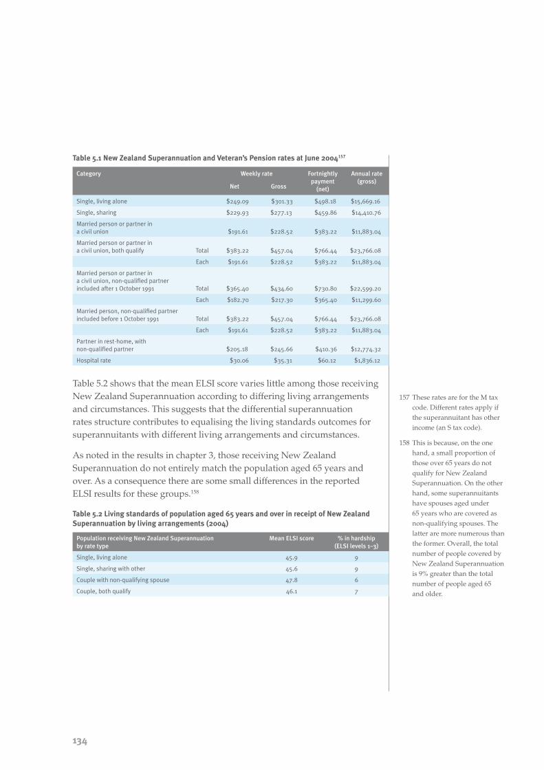
134

Table 5.2 shows that the mean ELSI score varies little among those receiving New Zealand Superannuation according to differing living arrangements and circumstances. This suggests that the differential superannuation rates structure contributes to equalising the living standards outcomes for superannuitants with different living arrangements and circumstances.

As noted in the results in chapter 3, those receiving New Zealand Superannuation do not entirely match the population aged 65 years and over. As a consequence there are some small differences in the reported ELSI results for these groups.158

Table 5.1 New Zealand Superannuation and Veteran’s Pension rates at June 2004157

Category Weekly rate Fortnightly payment

(net)

Annual rate (gross)

Net Gross

Single, living alone $249.09 $301.33 $498.18 $15,669.16

Single, sharing $229.93 $277.13 $459.86 $14,410.76

Married person or partner in a civil union $191.61 $228.52 $383.22 $11,883.04

Married person or partner in a civil union, both qualify Total $383.22 $457.04 $766.44 $23,766.08

Each $191.61 $228.52 $383.22 $11,883.04

Married person or partner in a civil union, non-qualified partner included after 1 October 1991 Total $365.40 $434.60 $730.80 $22,599.20

Each $182.70 $217.30 $365.40 $11,299.60

Married person, non-qualified partner included before 1 October 1991 Total $383.22 $457.04 $766.44 $23,766.08

Each $191.61 $228.52 $383.22 $11,883.04

Partner in rest-home, with non-qualified partner $205.18 $245.66 $410.36 $12,774.32

Hospital rate $30.06 $35.31 $60.12 $1,836.12

These rates are for the M tax code. Different rates apply if the superannuitant has other income (an S tax code).

This is because, on the one hand, a small proportion of those over 65 years do not qualify for New Zealand Superannuation. On the other hand, some superannuitants have spouses aged under 65 years who are covered as non-qualifying spouses. The latter are more numerous than the former. Overall, the total number of people covered by New Zealand Superannuation is 9% greater than the total number of people aged 65 and older.

157�

158�

Table 5.2 Living standards of population aged 65 years and over in receipt of New Zealand Superannuation by living arrangements (2004)

Population receiving New Zealand Superannuation by rate type

Mean ELSI score % in hardship (ELSI levels 1–3)

Single, living alone 45.9 9

Single, sharing with other 45.6 9

Couple with non-qualifying spouse 47.8 6

Couple, both qualify 46.1 7

135


Housing tenure

Home ownership or equity in a home is one of the most important assets that older people possess in New Zealand. It has, for the current cohort of older New Zealanders, meant that housing costs have been able to be minimised and this has been a significant determinant of living standards for older people.159

In 2004 older people who owned their own homes had the highest average living standards and were less likely to be in hardship than those who rented (see figure 5.6). Those who rented from Housing New Zealand (HNZC) tended to have the lowest average living standards and were more likely to be in hardship.

Fergusson et al. 2001.159�


13 18 46 23



7 11 43 40 1 4 29 66

Housing tenure

Popu

lati

on p

erce

ntag

e

60

55

50

45

40

35

30

25

20

15

10

5

0

Figure 5.6 Living standards distribution of older New Zealanders aged 65 and over by housing tenure (2004)

Rented – HNZC

32

9

46

13

Rented – private landlord Owned

10

14

57

19

3 3

37

58

2000 percentage

Means




136

lIvIng standards of older new Zealanders by fInancIal characterIstIcs

Chapter 3 showed that income, asset position and housing costs are strongly associated with the living standards of the wider New Zealand population. These factors are also associated with variation in the living standards of older New Zealanders.

Income

As with the population as a whole, the average living standards of older New Zealanders increased as their equivalent disposable incomes increased. Furthermore, the likelihood of hardship fell as incomes increased (see figure 5.7).

However, 85% of the older people within the lowest income category ($10,000 or less equivalent disposable income) still had comfortable or better living standards.

The only statistically significant change in average living standards is a moderate fall of 2 ELSI points for those with equalivised incomes between $10,001 and $20,000.

137


Asset position

Among older people, as with the general population, the value of the assets owned is strongly associated with living standards. The average living standards of older people increase as the value of owned assets increases (see figure 5.8). The generally favourable living standard position of older people is reflected in the finding that even for those in the lowest asset category ($10,000 or less) 81% have comfortable or good living standards. The great majority of older people who do not have good living standards are in the bottom asset category. For those with assets over $100,001 only 1% were experiencing some degree of hardship.


3 8 42 47


2 6 36 56


1 1 15 83


0 0 2 98

Equivalent disposable income

Popu

lati

on p

erce

ntag

e

80

75

70

65

60

55

50

45

40

35

30

25

20

15

10

5

0

$10,000 or less

9

5

47

38

$10,001 – $20,000 $20,001 – $40,000 $40,001 or higher

5 5

49

42

23

16

78

02

29

69

Figure 5.7 Living standards distribution of older New Zealanders aged 65 years and over by equivalent disposable income of the EFU (2004)

2000 percentage

Means




138

Housing costs

Most older New Zealanders have comparatively low housing costs compared with the rest of the population, due to the large number who own their own homes mortgage free or as part of a family trust.

Figure 5.9 shows that the general pattern observed with housing costs is that those with very high costs ($200 or more per week) tend to have lower average living standards than those with lower housing costs. This is likely to reflect the fact that those with higher housing costs are more likely to be paying rent or mortgages on capped incomes.


4 9 43 44


1 4 31 64


0 1 26 72


0 1 10 89

Asset value

Popu

lati

on p

erce

ntag

e

85

80

75

70

65

60

55

50

45

40

35

30

25

20

15

10

5

0

Figure 5.8 Living standards distribution of older New Zealanders aged 65 years and over by value of owned assets (2004)

$10,000 or less

109

55

26

$10,001 – $25,000 $25,001 – $100,000 $100,001 or more

2 2

33

62

1 2

37

60

0 1

17

83

2000 percentage

Means




139


Weekly housing costs

Popu

lati

on p

erce

ntag

e

65

60

55

50

45

40

35

30

25

20

15

10

5

0

Nilmean ELSI 45.9

7

1

31

61

$1 – $199mean ELSI 46.1

$200 or moremean ELSI 37.8

34

39

54

23

10

35

31

Figure 5.9 Living standards distribution of older New Zealanders aged 65 years and over by weekly housing costs (2004)




140

prIvate provIsIonIng for adequate lIvIng standards

The living standards research indicates that given the private provision for retirement that the current cohort of older people has made, New Zealand Superannuation and associated payments are sufficient to enable the majority of older people to avoid hardship. The living standards research does not specifically investigate whether older people have been able to maintain their previous working-age living standard in retirement. However, it is tentatively suggested that the majority of the current cohort of older people have probably maintained their pre-retirement living standards.160

The government housing policies between the 1930s and the 1970s were of particular relevance to the cohort of New Zealanders aged 65 years and over in 2000. These policies gave access to homeownership, through subsidised state loans, to many people who might not otherwise have been able to achieve it.161 These policies may therefore have significantly reduced the proportion of older people in hardship, as people were able to purchase homes during their working lives, resulting in low housing costs upon retirement.

The current generation of older people predominantly have comfortable or good living standards with less than one-tenth in hardship. However, additional analysis of living standards has demonstrated that having at least some level of private provision (including homeownership) contributes to the low level of hardship. Those who have no income additional to New Zealand Superannuation, have financial assets of $1,000 or less in total value, and who live in private market rental accommodation162 are four times more likely to be in hardship than older people generally and 13 times more likely than those with all three types of the listed private provisions.163

Emerging trends indicate that to maintain the distribution of living standards of older people in the future, current working-age people need to accumulate more assets than the previous cohort to potentially offset such factors as:

an increased life expectancy and therefore a longer retirement period to resource

delay and reduction in inheritances received due to increased life expectancies of older generations

an increased likelihood of events such as separation and divorce

an increased likelihood of needing to care for dependent elderly and dependent children during the same period.

•

•

•

•

Hong and Jensen 2003.

Ferguson 1994.

This constituted less than 5% of the older people population.

Hong and Jensen 2003.

160�

161�

162�

163�

141


Rearing fewer children could potentially enhance the distribution of living standards for future cohorts of older people by making more income available for asset accumulation. However, this would only occur if the additional income available was not required to offset the factors listed above. A level of asset accumulation would also be required that mirrored income levels if pre-retirement living standards were to be maintained. In particular, an emerging trend of reduced homeownership means that, for those who choose not to purchase their own home, alternative asset accumulation options need to be adopted to offset increased housing costs in retirement.164

A substantial change to the profile of the living standards distribution of older people will be the higher proportion of older Mäori and Pacific peoples, the majority of whom will have low living standards should the current disparity evident for these groups continue. In addition, the assistance provided to older people with low working-life incomes, and homeownership incentives through state loan subsidies from the 1930s to the 1970s, may have provided a strong boost to the asset accumulation of older people. However, this opportunity is not generally available to current working-aged people.

These trends suggest that the pattern of asset accumulation that has been successful over the working lives of the current older population may not necessarily transfer successfully to future cohorts.

Two key areas of focus for encouraging adequate private provision for retirement and thus adequate living standards in retirement include:

the ongoing promotion of savings behaviour and asset accumulation

the need to investigate ways of assisting people with low incomes to accumulate assets for retirement (whether in the form of homeownership or otherwise).

•

•

Hong and Jensen 2003.164�

142

summary

The survey indicated that older New Zealanders generally have good living standards and the risk of hardship is lower than it is for the population as a whole. This is consistent with the conclusions of MSD’s 2001 report Living Standards of Older New Zealanders.165

The living standards of older New Zealanders increase as age increases and there is little difference between older men and older women in terms of living standards.

Between 2000 and 2004 there was little change in the proportions of older New Zealanders in some degree of hardship. More older New Zealanders tended to have “comfortable” rather than “good” living standards in 2004 compared with 2000.

Owning one’s own home continues to be a factor associated with good living standards amongst older New Zealanders, as does having assets and limiting one’s housing costs.

Older New Zealanders who rent, have high housing costs and have few assets are more likely to be in hardship than other older New Zealanders. This suggests that current targeted income support provisions such as the Accommodation Supplement are critical to maintaining adequate living standards for older New Zealanders in need.

Past policies that have assisted homeownership and asset accumulation among the current cohort of older New Zealanders have contributed to their current favourable living standards distribution relative to the working-age population.

Changes in social, demographic and economic trends suggest that the substantial level of asset accumulation that occurred over the working lives of most people in the current older population may not be repeated in future cohorts. Fergusson et al. 2001.165�

143

Two key areas of focus for encouraging adequate private provision for retirement and thus adequate living standards in retirement include:

the ongoing promotion of savings behaviour and asset accumulation

the need to investigate ways of assisting people with low incomes to accumulate assets for retirement (whether in the form of homeownership or otherwise).

Future research that will aid understanding of the adequacy of private provision for retirement and living standards outcomes for future cohorts of older New Zealanders includes the longitudinal research currently underway (Statistics New Zealand’s Survey of Family Income and Employment) and modelling of asset accumulation scenarios and potential retirement outcomes.

•

•

145

Living standards of the low-income population 6

People within the low-income population have markedly different living standards (that is, even when income is controlled for) depending on whether their income source is an income-tested benefit, market income or New Zealand Superannuation.

Of the low-income population, those receiving income-tested benefits have the lowest average living standards while those receiving New Zealand Superannuation have the highest average living standards.

The result for New Zealand Superannuitants shows that even those with little additional income generally have a favourable living standard, with an ELSI mean that is above that of the overall population.

Income-tested beneficiaries have a moderately lower average living standard in 2004 than 2000 and a substantially higher proportion is in “severe hardship” (29% compared with 18%).

The large differences between the low-income groups reveal the importance of factors additional to income in influencing living standards, especially for people with limited incomes.

Initial analysis suggests that some of the factors contributing to living standard differences within the low-income population may be:

homeownership (positive effect on living standards)

assets of other types (positive effect)

economic family units (EFUs) with dependent children (negative effect)

marriage break-up (negative effect)

adverse adult life events generally (negative effect)

restrictions in social and economic participation caused by a serious health condition (negative effect).

•

•

•

•

•

•

–

–

–

–

–

–

Key points

Living standards of the low-income population

146

IntroductIon

Over recent years, there has been a change in the characteristics of the bottom third of the income distribution, with a growing proportion of this group consisting of income-tested beneficiaries.

There has been a long-standing interest in how those with low incomes have been faring. Research on this has included analyses of the shape of the income distribution, the characteristics of those whose incomes fall below particular thresholds, and changes in the incomes of particular subgroups of the population in relation to others.166 This type of work provides useful information on trends and can be based on routinely collected statistical information (for example, information collected by Statistics New Zealand’s Household Economic Survey). Its limitation is that it does not recognise that families with the same income can have differing living standards (resulting from differences in their levels of financial assets, levels of debt, etc), and it does not take account of differences in incomes among those below a particular income threshold.167

The analysis presented in this chapter examines the living standard scores of those in EFUs where the equivalent disposable income168 places them in the low-income range of the distribution of equivalent disposable income. In the 2000 survey, the bottom third of the income distribution was defined as low-income. This definition was used after analysis found it ensured a large enough sample for the examination of distinct sub-populations within the low-income group. For the 2004 survey, a similar definition has been employed. The low-income level is benchmarked at the 33rd percentile of the equivalent disposable incomes in the 2004 survey. The benchmark is then Consumer Price Index-adjusted to the 2000 dollar to identify the comparison group from the 2000 survey.169

Because of the policy interest in low-income families, in this chapter the low-income group has been further subdivided by income source into three mutually exclusive groups, introduced in chapter 3.

Income-tested benefit specified here as people in EFUs where there was receipt of an income-tested benefit (core benefit) in the last 12 months and no one was in full-time employment at the time of the survey.

New Zealand Superannuation specified here as people in EFUs where there was receipt of New Zealand Superannuation.170

Market income specified here as people in EFUs in neither of the above two categories and therefore receiving income primarily from market sources.171

•

•

•

Podder and Chatterjee 1998; Krishnan, Jensen and Ballantyne 2002.


Equivalent income is introduced in chapter 3.

Of the 2000 sample, 37.5% had real equivalent disposable incomes below the 2004 threshold.

The population in receipt of New Zealand Superannuation and those aged 65 years and older are not exactly the same. This is because, on the one hand, a small proportion of those over 65 years do not qualify for New Zealand Superannuation. On the other hand, some superannuitants have spouses aged less than 65 years who are covered as non-qualifying spouses. The latter are more numerous than the former. Overall, the total number of people covered by New Zealand Superannuation is 9% greater than the total number of people aged 65 and older.

Income source is defined using a prioritised classification. Some of the population here may have been in receipt of an income-tested benefit at some time during the past 12 months, but were full-time employed at the time of the survey. Similarly, superannuitants may have received an income-tested benefit before qualifying for New Zealand Superannuation during the year. Some in the income-tested benefits group may also have received income from market sources during the year but were not in full-time employment at the time of the survey.

166�

167�

168�

169�

170�

171�

147


overall dIstrIbutIon

New Zealand Living Standards 2000172 identified variation in living standard outcomes between those on similar incomes. Figure 6.1 shows that this pattern continues in 2004, with representation in all seven ELSI levels.


An asterisk printed by the difference indicates that the difference in ELSI means between 2000 and 2004 is significant at the 95% confidence level, ie a p-value less than 0.05. Appendix C reports the confidence intervals for the 2004 mean ELSI, and statistical significance for changes in means, hardship and “severe hardship”.

Proportions in hardship and differences in the mean ELSIs reported are calculated from unrounded numbers. Therefore they may differ from the sum of the proportions given in the figures.

172�

173�

174�

Despite this variation, there was a large contrast in living standard distribution between those in the low-income group and the top two-thirds of the income distribution. Those in the low-income category had considerably lower living standards than the remainder of the population, with a mean ELSI score 12.3 points lower. In fact, of those in the low-income group, 45%174 are experiencing some level of hardship, denoted by ELSI levels 1–3, whilst 14% have “good” or “very good” living standards (levels 6 and 7). This situation reverses when the living standards of the rest of the population are examined, with just 13% in some level of hardship and 45% having “good” or “very good” living standards.

Comparing the 2004 results with those for 2000, the average living standards of EFUs in the total population stayed stable, while the average living standards of the low-income population fell slightly. Further, those experiencing some degree of hardship within the low-income population increased from 40% in 2000 to 45% in 2004. Of further concern is the increase in the proportion of low-income New Zealanders experiencing “severe hardship” (10% in 2000 up to 17% in 2004).

Low income (bottom third)

Equivalent disposable income

Popu

lati

on p

erce

ntag

e

35

30

25

20

15

10

5

0

Figure 6.1 Living standards distribution of total population by the equivalent disposable income of the EFU (2004)173

17

1315

19

22

13

1 24

7

14

27

33

12

Top two-thirds


10 13 17 20 21 3 0 1 3 9 13 24 38 13



2000 percentage

Means

148

varIatIon by Income source

While the living standard scores of those in the low-income category were lower than the population as a whole, there was wide variation between the scores of those in the low-income category depending on their source of income. This is shown in figure 6.2.

Overall, those on income-tested benefits had lower average living standards than those receiving market incomes, who in turn had lower scores than those receiving New Zealand Superannuation. The average ELSI scores for these groups are 24.3, 33.3 and 42.7 respectively. Of those in receipt of an income-tested benefit, 65% had ELSI scores that placed them in one of the three lowest scale categories (in hardship). This proportion decreases to 41% for those receiving market incomes and declines further to 13% for those receiving New Zealand Superannuation. Only 4% of those receiving an income-tested benefit had ELSI scores that placed them in the “good” living standards category (none had “very good” living standards). This proportion increased to 14% for those receiving market incomes and increased further to 37% for those receiving New Zealand Superannuation.

Although by definition all three subgroups have incomes in the low-income range, there is still the possibility of their having somewhat different income distributions. The question arises whether this is so, and whether any such differences in income account for the living standard differences shown in figure 6.2.

31

Income-tested benefits

Income source

Popu

lati

on p

erce

ntag

e

40

35

30

25

20

15

10

5

0

Figure 6.2 Living standards distribution of the low-income population by the income source of the EFU (2004)

29

22

14

19

12

4

Market income

12

9

1920

25

13

New Zealand Superannuation

18 19 7 12 1 2


6 13 29 44 618 24 23 1321 20 16 5

2

56

16

3433

4

01




2000 percentage

Means

149


Examination of the incomes of the subgroups showed that there were small differences between the means, with the income-tested beneficiaries having the lowest mean income and the low-income superannuitants having the highest mean income. The effect of these differences on the living standard results for the subgroups was estimated using a linear regression model.175 The model indicated that the ELSI difference of 18.4 between the beneficiary subgroup mean and the superannuitant subgroup mean would have been 16.8 in the absence of the income difference; in other words, the higher incomes of the superannuitants accounted for only a small part of the living standard difference (1.6 ELSI points out of 18.4 points). When the difference between the beneficiary and market income subgroups was similarly analysed, it was found that the ELSI difference of 9.0 would have been 9.3 in the absence of the income difference. The ELSI difference of 9.4 between the market income and superannuitant subgroups would have been 7.5 in the absence of the income difference. The estimates indicate that while there are some differences in incomes between the three subgroups, those small income differences account for only a very modest part of the very large living standard differences between the subgroups.

Comparisons between 2004 and 2000 show that the mean living standards scores for beneficiaries fell moderately, and the beneficiary and market income groups saw increases in the proportion experiencing “severe hardship”. However, the most marked increase in “severe hardship” was for beneficiaries (from 18% in 2000 to 29% in 2004). For low-income superannuitants, the most significant change in the living standards distribution was redistribution from “good” in 2000 to “comfortable” in 2004. For the low market income subgroup, the most notable change was an increase in the proportion experiencing “severe hardship” – from 7% in 2000 to 12% in 2004.

The effect of the income differences on the ELSI scores of the subgroups was estimated using a linear regression between ELSI scores (the dependent variable) and a set of 19 independent variables, one of which was the log of the equivalent disposable income. Other independent variables included economic factors such as the value of assets, the ratio of housing costs to income, whether the respondent was self-employed, personal characteristics (eg ethnicity, educational qualifications), and features of the EFU (eg whether it was part of a household containing other EFUs). The model was specified for the population as a whole and fitted using the weighted survey data. The regression had an adjusted R2 of 0.47 (indicating that the independent variables accounted for almost half of the variation in ELSI scores). This regression provides a relatively strong basis for estimating the effect of the income differences between the subgroups on the ELSI differences. If the procedure mis-estimates the effect of the income differences, it is likely to over-estimate them. The analysis provides a secure basis for concluding that the income differences between the subgroups account for only a small part of the large ELSI differences between them.

175�

150

varIatIon by fInancIal, socIal, demographIc and adversIty characterIstIcs

The previous section has shown that there are large differences between the living standards of the three low-income subgroups. The question arises as to what factors are associated with these differences. Earlier work on the living standards of older New Zealanders identified a number of variables such as income, housing costs, tenure, asset position and education as being associated with variations in living standards amongst older New Zealanders. Previous chapters have shown that these and other social, demographic, financial and adversity factors are also associated with variation in living standards found amongst the population as a whole.

Table 6.1 gives comparisons between the three low-income subgroups in terms of a number of these factors.

Table 6.1 Composition of low-income subgroups by financial, social and demographic characteristics (2004)

Low-income population

Income-tested beneficiaries (% of group)

Market incomes (% of group)

Superannuitants (% of group)

Total low-income population

(% of group)

Number of types of assets176

Three or more 4 11 19 11

Housing tenure

Owned 40 51 88 53

Housing cost outgoings to income ratio (HOTI)

HOTI ≤ 30% 50 62 88 62

EFU type

Single adult or couple without dependent children 34 39 97 48

Ethnicity

Not Mäori or Pacific ethnicity 59 67 92 68

Highest educational qualification of respondent

Tertiary qualification 12 22 4 14

Region

Living outside main urban areas 28 26 44 30

Marriage break-up177

None 46 75 81 67

Life shocks

None 8 33 20 22

Number of types of payments causing financial difficulties

None 26 31 70 41

Number of types of restrictions in social and economic participation caused by serious health problems

None 59 80 56 67

Asset types include: money deposited with banks, eg savings, cheque accounts, term deposits; other investments, eg shares, unit trusts, bonus bonds, debentures, credit unions; life insurance policies, eg whole life endowment, investment-linked policies; money or investments in a family trust; money owed to respondent; residential property, eg holiday home, rented-out residential property, land; investment in commercial property; business ownership or investment, eg in farming, forestry or any other business; any other assets, eg art, antiques, collectibles.

As explained in chapter 3, the term marriage break-up is used in this report to refer to the break-up of a marriage or a relationship in the nature of a marriage. That is to say, the term encompasses the break-up of both de facto and de jure relationships.

176�

177�

151


Table 6.1 shows that for most of the variables there is a clear gradient between income-tested beneficiaries, those with low market incomes and low-income superannuitants. For example, the proportions of people with three or more different types of assets are 4% (of the beneficiary subgroup), 11% (of the low market income subgroup) and 19% (of the low-income superannuitant subgroup). The proportions of people in the three subgroups who own their own homes are 40% (beneficiaries), 51% (market incomes) and 88% (superannuitants). As indicated by these figures, on most of the variables the beneficiary subgroup is the worst off and the low-income superannuitant subgroup is the best off.

There are, however, some departures from this pattern. The variables that show different patterns are tertiary qualifications, region, life shocks and restrictions due to a serious health condition.

The low-income superannuitants are the least likely to have tertiary qualifications, reflecting the rise in educational acquisition over recent years. Similarly reflecting the relatively greater age of that subgroup, the superannuitants are more likely than the low market income subgroup to have had life shocks and to be subject to restrictions caused by ill health. The departure from the common pattern for the regional variable arises because the likelihood of being in a main urban area is slightly higher for the market income subgroup than for the beneficiary subgroup. This may reflect the strong labour demand in those areas.

Appendix E gives detailed breakdowns for the variables used in table 6.1, together with ELSI means and hardship percentages for the breakdown categories.

152

factors related to dIfferences In lIvIng standards between low-Income subgroups

The figures given in table 6.2 show that there are notable differences between the three low-income subgroups in terms of a number of variables that have been found to correlate with living standards. It is of interest to advance the analysis, so that we may examine the extent to which those differences may contribute to the large living standard differences between the subgroups. This has been done by calculating the ELSI means for the subgroups after standardisation with respect to each of the previously examined variables. The standardisation procedure applied is the same as that used by health statisticians to produce, for example, age-standardised mortality rates. These standardised rates show what the levels of mortality would be in different populations if they all had the same age structure (ie all had the same proportions of infants, children, adolescents, older people, etc).

To make standardisations of this type, it is necessary to specify a “reference population”, whose distributions, with respect to the standardisation variables, provide the basis of the procedure. In this instance, the low-income superannuitant subgroup has been used as the reference population. This is the least disadvantaged of the subgroups. The standardisations thus give results that are indicative of how the living standards of the other subgroups would be affected if they were in the more favourable position of the low-income superannuitants, with respect to the standardisation variables.

The way to interpret the standardised ELSI means can be illustrated by way of a particular example, which relates to the value given for the mean ELSI score for the beneficiary subgroup after standardisation for the number of types of assets. This value, 31.0, is the mean ELSI score that would be expected if the beneficiary subgroup had the same distribution as the superannuitant subgroup with respect to the number of types of assets. The unstandardised mean is 24.3. The standardised mean is higher because there is a positive relationship between living standard and number of types assets, and the superannuitant subgroup has a more favourable distribution of number of types assets. For the low market income subgroup, the standardised mean (37.7) is also higher than the unstandandarised mean (33.3), although the difference between the two is not as great as it was for the beneficiary subgroup.

153


Table 6.2 Low-income subgroups: Mean living standard scores standardised for relevant demographic, economic and social variables178

Mean ELSI score

Mean ELSI score standardised for:

EFU type number of types of assets179

number of life shocks

number of marriage

break-ups

number of types of restric-tions in

social and economic

partici-pation

caused by serious health

problems

housing tenure type

educa-tional

qualifica-tion

ethnicity housing cost

outgoings to income

ratio (HOTI)

region

Beneficiaries 24.3 32.3 31.0 28.6 28.4 28.3 27.8 26.6 25.7 25.6 24.9

Market incomes 33.3 38.2 37.7 35.4 35.9 34.7 36.4 33.2 35.0 33.1 33.8

New Zealand Superannuitants

42.7 42.7 42.7 42.7 42.7 42.7 42.7 42.7 42.7 42.7 42.7

For the beneficiary subgroup, the standardisation for EFU type produces the biggest upwards adjustment to the ELSI mean. In essence, this standardisation estimates what the beneficiary mean would be if only 3% of beneficiaries were caring for dependent children (that being the proportion of superannuitants caring for children) rather than 67%. The large effect associated with this standardisation points to the costs of children as being a major contributor to the very low living standards of the beneficiary subgroup. Other standardisations that produced substantial adjustments are those for number of types of assets, number of life shocks, number of marital break-ups, number of types of restrictions caused by serious health conditions and type of housing tenure. The standardisations referred to above are also the ones that produce the biggest adjustments for the low market income subgroup.

It is necessary to take some caution in interpreting the standardisation results. Because the standardisations are made independently of one another, they do not take account of the interrelationships between the variables involved. Thus it is possible for an effect that is identified with a particular variable to arise from the influence of other variables with which it is correlated. To further complicate matters, some of the significant other variables may be absent from the analysis. They may be causally important omitted variables that have only an unidentified, reflected presence in the results through their correlations with the variables that have been included.

The standardisation procedure used for each of the variables applies the distribution of the low-income superannuation subgroup for each variable to each of the other subgroups, thereby producing a standardised mean ELSI score for that variable.

Asset types include: money deposited with banks, eg savings, cheque accounts, term deposits; other investments, eg shares, unit trusts, bonus bonds, debentures, credit unions; life insurance policies, eg whole life endowment, investment-linked policies; money or investments in a family trust; money owed to respondent; residential property, eg holiday home, rented-out residential property, land; investment in commercial property; business ownership or investment, eg in farming, forestry or any other business; and other assets, eg art, antiques, collectibles. This does not include the family home.

178�

179�

154

For those reasons, the results do not permit unequivocal conclusions to be drawn about the reasons for the living standard differences between the subgroups. Nonetheless, the results are suggestive of the conclusion that the factors that have been highlighted (ie responsibility for children, assets, life shocks, marital break-ups, restrictions caused by health problems and housing tenure) may well contribute to the differences.

155


summary

In this chapter the low-income population was broken down into three subgroups on the basis of the source of income. The three subgroups consist of people receiving income-tested benefits, people with low market incomes, and low-income superannuitants. The three subgroups had greatly differing living standards. The beneficiary subgroup had a very depressed living standard distribution (with a mean ELSI score of 24.3), while the low-income superannuitant subgroup had a distribution that was slightly more favourable than the overall population (with a mean of 42.7). The distribution for the low market income subgroup was between the other two (with a mean of 33.3).

Although there were modest income differences between the three subgroups, those differences did not substantially account for differences in living standards.

An initial examination was made of the extent to which the differences between the subgroups, in mean ELSI scores, were associated with differences between them in various demographic, economic and social variables. This was done using a standardisation procedure. It was found that the ELSI differences between the subgroups were associated with differences in EFU type, assets, life shocks, marital break-ups, restrictions caused by health problems and housing tenure. The results do not establish unequivocally that these variables contribute to the differences but point towards that conclusion.

157

7

Concluding comments

This report extends an earlier study of living standards undertaken in 2000. It uses new survey data, collected in 2004, to update the earlier picture of the living standards of New Zealanders, and examines the changes that have occurred. In addition, it offers new insights into living standards by presenting results obtained from new survey questions on various types of adversities. The report uses the Economic Living Standards Index (ELSI), a scale developed to directly measure the living standards of New Zealanders.

Current living standards

The ELSI scores for the population as a whole show that New Zealanders have a generally favourable distribution of living standards. More than three-quarters of the population have living standards that are comfortable or good.

Comparatively high average living standards scores are found among:

New Zealanders aged 45 years and over (including those in receipt of New Zealand Superannuation)

couples without children

mortgage-free homeowners

people with tertiary qualifications

people working as legislators, administrators, managers or professionals and those in agricultural occupations

people with income from self-employment

people with equivalent disposable incomes of $30,001 or higher

people with assets over $10,001

people who have not had a marriage break-up

people who have not experienced adverse life events (life shocks)

people who do not have any restrictions in social and economic participation due to serious health problems

people who do not have any types of payments which are causing them financial difficulties.

•

•

•

•

•

•

•

•

•

•

•

•

158

In contrast, comparatively low average living standard scores are found among:

low-income families with children

Mäori and Pacific New Zealanders


people working in “elementary” (unskilled) occupations

those receiving income-tested benefits

New Zealanders with few or no assets

women who have had a marriage break-up

people who have had multiple life shocks

people with multiple restrictions in social and economic participation due to serious health problems

people with multiple types of payments that are causing them financial difficulties.

Of particular concern are the positions of beneficiary families with children, Pacific people and those renting from Housing New Zealand. These groups have low average living standards, with high proportions in “severe hardship”.

The primary goal of this report has been to set out the pattern of living standard differences in New Zealand rather than to explain those differences (which will be the next stage of MSD’s Living Standards Research Programme). Nonetheless, results from the analysis of people with low incomes offer strong indications of some of the factors that are involved. Those results point strongly to the importance of costs associated with having children, not having financial assets, not owning one’s own home, and the experience of life shocks, marriage break-up and restrictions due to health problems. Additionally, income only accounted for a small difference in living standards across subgroups within the low-income population. The results suggest that, where very low living standards occur, they are not commonly a result of a single factor but reflect the compounding impacts of multiple disadvantages. This compounding appears to be particularly severe in the case of income-tested beneficiary families with dependent children.

•

•

•

•

•

•

•

•

•

•

159

Concluding comments 7

Patterns of change

In commenting on the differences between results for 2000 and 2004, we have drawn attention to the potential for ELSI scores to be affected by changes in general expectations about access to consumption. This is because the score effectively gives a measure of the extent to which a person’s consumption (in the relevant areas) corresponds to what they would like it to be. In other words, the ELSI scale, despite being based on items about particular types of consumption, has a relative aspect. Scores at any particular time are likely to be, in part, a reflection of the extent to which contemporary expectations are met for access to consumption goods.

Analysis of questions relating to ownership of consumer items, and to types of consumption relating to social participation, indicates that there has been a small increase in what people have and do, but a slightly greater increase in what people want (expectations). This suggests that overall expectations have run slightly ahead of the small rise in consumption. The consequence of this is that the 2004 ELSI scores are likely to be a little lower than they would otherwise have been. The size of the effect has been estimated, although this has involved assumptions that cannot be tested directly. The estimate suggests that scores for 2004 are one to two ELSI points lower than they would otherwise have been. The effect of the rise in expectations is therefore small or negligible.

The change in expectations is broadly similar for the various types of subgroups considered in the report (ie ethnicity groups, age groups, different family types, etc). Thus the rise in expectations can be expected to have had a relatively uniform effect in slightly lowering the ELSI scores obtained in 2004.

A comparison of the 2004 and 2000 results suggests that overall living standards have changed little over the period. Mean ELSI scores were approximately one ELSI point lower in 2004. The analysis of the effect of rising expectations suggests that if expectations had not changed, the mean ELSI score recorded for 2004 might have been up to one ELSI point higher than for 2000. Although this is the case, a change of one ELSI point either way is described as “very small” or “negligible”.

The relative positions of the various subgroups remain much the same in 2004 as 2000.

160

For example, in both years Mäori and Pacific people, low-income families, people with few assets and larger families have lower living standards than the population as a whole; while couples without children, older people, self-employed people and those with assets have higher living standards.

Although the overall average has changed little, there has been some increase in the level of living standards inequality within the population. Related to this, there has been an increase in disparities between groups, with the groups with low living standards falling further behind those with high living standards. Furthermore, the general increase in inequality has occurred to an exaggerated extent amongst the groups with low living standards. As a consequence, the latter groups – for example, Mäori and Pacific people, beneficiaries and low-income families with children – have shown increases in the proportions of people in “severe hardship”.

Groups for which living standards were lower in 2004 than 2000 include:

large families (three or more dependent children)


people with low equivalent incomes

people with few assets

people in receipt of an income-tested benefit, especially those with dependent children.

The increases in disparity in living standards across the population have primarily been due to greater within-group variation in living standards. For example, there is a greater spread of living standards among Mäori, with a higher proportion in hardship and a higher proportion with good living standards. The increasing diversity of living standards is also shown for children and families with dependent children, indicating that outcomes vary depending on other factors associated with families with children.

A buoyant economy and record low unemployment has possibly contributed to this greater variation and increased disparity. It has created opportunities which many have been able to take advantage of. However, the resulting gains have been unevenly spread, with those unable to take advantage of these circumstances possibly in a more disadvantaged position than those who have been able to take full advantage of the economic conditions. It is important to note that not all of the effects of the recent positive economic environment will be indicated in the current survey. There is almost certainly a lag between the falling unemployment rate for example and overall living standards. Also some of the changes in the economy occurred after the survey period.

•

•

•

•

•

161


Policy implications

Some of the findings in this report have important implications for government social policy. It is not the purpose of this report to offer prescriptions, but it is useful to flag some of these implications as they provide an illustration of the relevance of this type of living standards research to social policy.

The generally favourable living standards of older New Zealanders suggest that current support arrangements are meeting the needs of the majority of superannuitants. However, this does not reduce the need for further development of policies providing targeted assistance to the minority of superannuitants with inadequate living standards. Further, the results support the continued focus on planning for retirement through the accumulation of financial assets (including homeownership) during the working years. Without adequate preparation,180 there is no guarantee that the level of material wellbeing of the current generation of older New Zealanders will also be achieved by future generations.

The results in the report vividly reinforce previous knowledge concerning the higher prevalence of disadvantage among Mäori and Pacific people. The results underline the importance of maintaining a strong focus on finding effective ways of reducing these disparities. This issue is particularly urgent in relation to Pacific people, who have a higher prevalence of “severe hardship” in 2004 than in 2000.

The results also highlight the relatively poor living standards of many beneficiary children (who are predominantly in sole-parent families). More than 30% of these children are in “severe hardship”. Furthermore, children of beneficiaries in 2004 had lower living standards than such children in 2000. There is considerable evidence concerning the high social costs of hardship amongst children, which can have lasting negative effects through compromising their development. Thus effective policy interventions – both preventive and remedial – deserve attention not only on the basis of advancing social justice, but also because they have the potential to give high returns on expenditure.

For example, private asset accumulation.

180�

162

In this connection, it is relevant to record that the government is currently carrying out an extensive programme of welfare reforms. These include the Working for Families initiatives directed at beneficiaries and low-income working families. The first of these changes was implemented on 1 October 2004. Further stages were implemented in April 2005, October 2005 and April 2006, and the final stage is set to come in on 1 April 2007. The reforms have the stated objectives of:

making work pay by supporting families with dependent children, so that they are rewarded for their work effort

ensuring income adequacy, with a focus on low- and middle-income families with dependent children to address issues of poverty, especially child poverty

achieving a social assistance system that supports people into work, by making sure that people get the assistance they are entitled to, when they should, and with delivery that supports them into, and to remain in, employment.

These reforms, together with macroeconomic conditions, will shape the pattern of family incomes over the following years. This report establishes some pre-reform benchmarks of living standards. To assist in gauging the effects of the Working for Families reforms, it is important to continue the sort of monitoring and analysis that is provided by the living standards research.

The report contains a variety of results that, taken together, point to the importance of multiple disadvantages as being a critical cause of hardship, especially “severe hardship”. Most measures for ameliorating or preventing disadvantage (ie accommodation assistance, assistance for child costs, disability assistance, tertiary study assistance, etc) relate to specific sources of disadvantage considered separately. While these measures provide a good general foundation for the system of social assistance, they do not recognise the compounding negative impact of multiple types of disadvantage. Some major future challenges arising from the report are to develop a better understanding of multiple disadvantage and its role in generating hardship and to find new policy approaches for grappling more effectively with the cumulative burden of multiple disadvantage. These tasks are particularly important in relation to income-tested beneficiary families, for the evidence presented here indicates that these families are constrained not only by relatively low incomes but, in many cases, also have to struggle with a range of other difficulties that in combination can drive them into “severe hardship”.

•

•

•

163


Explaining differences in living standards

The results in this report strengthen the knowledge base on which social policy rests and will be immediately useful in assessing priorities. They constitute a step up in our understanding of current needs for social assistance and the ways in which such assistance might best be targeted. However, the report is directed mainly towards giving a descriptive picture of living standards in this country and indicating how the picture has changed since 2000, when the earlier survey was carried out. While the report has pointed to some of the factors that affect living standards, and can help explain differences between individuals and groups, there has not been a full analysis of the interplay of relationships using a multivariate framework. MSD is currently undertaking such an analysis and plans to publish findings in 2007.

Dataset available to other researchers

The 2004 living standard survey produced a very rich dataset that contains information on many matters other than living standards. For example, it contains information about family structure, labour market participation, education, disability and health (to name just a few). MSD would like to see this information utilised as widely as possible to improve understanding of New Zealand life, and welcomes inquiries from bona fide researchers who wish to conduct their own analyses, whether extensions of those reported here or directed towards new topics and questions.181

Please address any queries regarding the data to: The manager, Social and Economic Wellbeing Evaluation Team, CSRE, Ministry of Social Development, PO Box 1556, Wellington, with the heading “Access to living standards data”.

181�

164

References

Ballantyne S, Chapple S, Maré D and Timmins J (2004) Movements into and out of child poverty in New Zealand: Results from the linked income supplement. MOTU Working Paper 03-13. MOTU Economic and Public Policy Research, Wellington, New Zealand.

Benefit Advocacy/Departmental Joint Working Group (2001) Closing the Gaps – Closing the Food Banks? Paper presented at the Fifth National Food Bank Conference, Wellington, New Zealand.

Booth C (1903) Life and Labour of the People of London. Macmillan, London.

Bray J R (2001) ‘Hardship in Australia: An analysis of financial stress in the 1998–1999 Australian Bureau of Statistics Household Economic Survey’. Occasional Paper No.4, Department of Family and Community Services, Australia.

Centre for Housing Research Aotearoa New Zealand (2005) Annual Report. Wellington, New Zealand.

Crampton P, Salmond C, Kirkpatrick R, Scarborough R and Skelly C (2000) Degrees of Deprivation in New Zealand: An Atlas of Socioeconomic Difference. David Bateman Ltd, Auckland, New Zealand.

Crews G (June 2004) AMP Home Affordability Report. Vol 14(3). Massey University and AMP Financial Services, New Zealand.

Cunningham C, Durie M, Fergusson D, Fitzgerald E, Hong B, Horwood J, Jensen J, Rochford M and Stevenson B (2002) Ngä Ähuatanga Noho o te Hunga Pakeke Mäori Living Standards of Older Mäori, Ministry of Social Development, Wellington, New Zealand.

Davey J (1993) From Birth to Death 3. Institute of Policy Studies, Victoria University of Wellington, New Zealand.

Davis P, McLeod K, Ramson M and Ongley P (1997) The New Zealand Socio-Economic Index of Occupational Status (NZSEI). Research Report No. 2, Statistics New Zealand, Wellington, New Zealand.

DTZ Research (2004) Housing Costs and Affordability in New Zealand. Centre for Housing Research Aotearoa New Zealand, Wellington, New Zealand.

Easton B (1995) ‘Poverty in New Zealand: 1981–1993’. New Zealand Sociology 10(2): 192–213.

Ferguson G (1994) Building the New Zealand Dream. Dunmore Press Ltd, Palmerston North, New Zealand.

165

References

Fergusson D, Hong B, Horwood J, Jensen J and Travers P (2001) Living Standards of Older New Zealanders: A Summary. Ministry of Social Policy, Wellington, New Zealand.

Ganzeboom H, DeGraaf P, Treiman D and DeLeeuw J (1992) ‘A standard international socioeconomic index of occupational status’. Social Science Research 21: 1–56.

Ganzeboom H and Treiman D (1996) ‘Internationally comparable measures of occupational status for the 1988 ISCO’. Social Science Research 25: 201–239.

Goh K (2005) ‘Savings and the Household Balance Sheet’. Reserve Bank Bulletin, Vol 68(2).

Gordon D, Adelman L, Ashworth K, Bradshaw J, Levitas R, Middleton S, Pantazis C, Patsios D, Payne S, Townsend P and Williams J (2000) Poverty and Social Exclusion in Britain. Joseph Rowntree Foundation, York.

Gordon D, Davey Smith G, Dorling D and Shaw M (Eds) (1999) Inequalities in Health: The evidence presented to the Independent Inquiry into Inequalities in Health. The Policy Press, Bristol.

Gray A (2004) Weighting Procedure and Proposed Variance Estimation for the Living Standards Survey. Statistics Research Associates Ltd, Wellington, New Zealand.

Harris P (2003) Savings: Policy Issues and Options. DTZ Research. http://www.isi.org.nz/files/Saving%20New Zealand%20-%20Discussion %20Paper.PDF

Health Utilisation Research Alliance (in press) ‘Ethnicity, socio-economic deprivation and consultation rates in New Zealand general practice’. Journal of Health Services and Research Policy.

Hollings D (2001) Of Gold Diggers and Possums. Paper presented at the 2001 Family Law Section Conference. http://www.familylaw.org.nz/advocate/econ-disparity.asp

Hong B and Jensen J (2003) Assessing the Adequate Private Provision for Retirement: A Living Standard Perspective. Ministry of Social Development, Wellington, New Zealand.

Housing New Zealand (1 November 2005) Email correspondence.

Hyslop D and Yahanpath S (2005) Income Growth and Earnings Variations in New Zealand 1998–2004. Treasury Working Paper 05/11, Wellington, New Zealand.

166

Immervoll H and Barber D (2006) Can Parents Affort to Work? Childcare Costs, Tax-Benefit Policies and Work Incentives. OECD Social, Employment and Migration, Occasional Papers No.31.

Jameson B and Nana G (2004) Furthering Our Understanding of Tenure Transition. Centre for Housing Research Aotearoa New Zealand, Wellington, New Zealand.

Jensen J, Spittal M, Crichton S, Sathiyandra S and Krishnan V (2002) Direct Measurement of Living Standards: The New Zealand ELSI Scale, Ministry of Social Development, Wellington, New Zealand.

Jensen J, Spittal M and Krishnan V (2005) ELSI Short Form: User Manual for a Direct Measure of Living Standards, Ministry of Social Development, Wellington, New Zealand.

Krishnan V (1995) ‘Modest but adequate: An appraisal of changing household income circumstances in New Zealand’. Social Policy Journal of New Zealand/Te Puna Whakaaro, 4: 76–97.

Krishnan V, Jensen J and Ballantyne S (2002) New Zealand Living Standards 2000. Ministry of Social Development, Wellington, New Zealand.

Krishnan V, Jensen J and Rochford M (2002) ‘Children in poor families: Does the source of family income change the picture?’ Social Policy Journal of New Zealand/Te Puna Whakaaro, 18: 118–147.

Krishnan V, Schoeffel P and Warren J (1994) The Challenge of Change: Pacific Island Communities in New Zealand 1986–1993. New Zealand Institute of Social Research and Development Ltd, Wellington, New Zealand.

Larsen V (2004) ‘Why earning more can make you poor’. North & South, 224: 42–50.

Mack J and Lansley S (1985) Poor Britain. George Allen and Unwin, London.

Market Economics Ltd (2003) The Economic Impact of the 2003 America’s Cup Defence. Ministry of Tourism, Wellington, New Zealand.

Mayer S E (2002) The Influence of Parental Income on Children’s Outcomes. Ministry of Social Development, Wellington, New Zealand.

Middleton S, Ashworth K and Braithwaite I (1997) Small Fortunes: Spending on children, childhood poverty and parental sacrifice. Joseph Rowntree Foundation, York.

Ministry of Economic Development (2003) Population and Sustainable Development. Ministry of Economic Development, Wellington, New Zealand.

167

References

Ministry of Social Development (2004) Children and Young People: Indicators of wellbeing in New Zealand. Ministry of Social Development, Wellington, New Zealand.

Ministry of Social Development (2005) The Social Report 2005. Ministry of Social Development, Wellington, New Zealand.

Ministry of Social Policy (2001) The Social Report 2001. Ministry of Social Policy, Wellington, New Zealand.

Ministry of Women’s Affairs (2001) Mäori Women: Mapping inequalities and pointing ways forward. Ministry of Women’s Affairs, Wellington, New Zealand.

Mowbray M (2001) Distributions and Disparity: New Zealand household incomes. Ministry of Social Policy, Wellington, New Zealand.

New Zealand Council for Christian Social Services (2003, 21 October) Crippling Levels of Debt Threaten Low Income Families [Media Release]. Wellington, New Zealand.

New Zealand Institute of Economic Research (2004) Update September 2004. New Zealand Institute of Economic Research, Wellington, New Zealand.

Nolan B and Whelan C (1996) Resources, Deprivation, and Poverty. Clarendon Press, Oxford.

Perry A, Douglas G, Murch M, Bader K and Borkowski M (2000) How Parents Cope Financially on Marriage Breakdown. Joseph Rowntree Foundation, York.

Podder N and Chatterjee S (1998) Sharing the National Cake in Post Reform New Zealand: Income inequality in terms of income sources. Paper presented to the New Zealand Association of Economists, Wellington, New Zealand.

Ringen S (1988) ‘Direct and indirect measures of poverty’. Journal of Social Policy, 17: 351–66.

Ringen S (1996) ‘Households, goods, and well-being’. Review of Income and Wealth, 42(4): 421–431.

Robins A (1996) ‘Statistics New Zealand Household Expenditure and Income Survey: What can it tell us about standard of living?’ Social Policy Journal of New Zealand/Te Puna Whakaaro, 6: 183–199.

Shaw M, Dorling D, Gordon D and Davey Smith G (1999) The Widening Gap: Health Inequalities and Policy in Britain. The Policy Press, Bristol.

168

Social Policy Agency (1994) Foodbanks in New Zealand: Patterns of growth and usage: A report on a short-term research investigation. Social Policy Agency, Wellington, New Zealand.

Social Policy Agency (1999) Social Environment Scan. Department of Social Welfare, Wellington, New Zealand.

Statistics New Zealand (1998a) Census of Population and Dwellings 1996 Employment and Unemployment. Statistics New Zealand, Wellington, New Zealand.

Statistics New Zealand (1998b) New Zealand Now: Mäori. Statistics New Zealand, Wellington, New Zealand.

Statistics New Zealand (2002) Pacific Progress: A report on the economic status of Pacific peoples in New Zealand. Statistics New Zealand, Wellington, New Zealand.

Statistics New Zealand (2005) [Household Economic Survey]. Unpublished data.

Statistics New Zealand (2005) Household Labour Force Survey (June 2005 quarter) – Hot Off the Press. Statistics New Zealand, Wellington, New Zealand.

Stephens R, Waldegrave C and Frater P (1995) ‘Measuring Poverty in New Zealand’. Social Policy Journal of New Zealand/Te Puna Whakaaro, 5: 99–112.

Stephens R, Frater P and Waldegrave C (2000) ‘Below the Line: An analysis of income poverty in New Zealand, 1984–1998’, Working Paper 2/00. Graduate School of Business and Government Management, Victoria University of Wellington, New Zealand.

TNS (2004) Living Standards Methodology Report. Ministry of Social Development, Wellington, New Zealand. http://www.msd.govt.nz/work-areas/social-research/living-standards/index.html

Townsend P (1979) Poverty in the United Kingdom: A survey of household resources and standards of living. Penguin, Harmondsworth.

Travers P and Richardson S (1993) Living Decently. Oxford University Press, Melbourne, Australia.

Treasury (2004) New Zealand Economic and Financial Overview 2004. Treasury, Wellington, New Zealand.

Valins O (2004) When Debt Becomes a Problem: A literature study. Ministry of Social Development, Wellington, New Zealand.

169

Appendix A: ELSI items and score calculation

Types of items

The items in the ELSI are of three types.

“Enforced lack” items, scored as 0 (an enforced lack) or 1 (no enforced lack).182 This is defined as: a person or EFU has an enforced lack when something wanted is lacked because of its cost. If the lack is due to any other reason, including it not being wanted, it is not an enforced lack.

The enforced lack items in ELSI are composed of two sets:

(a) those relating to ownership of personal and household goods (whose enforced lack is referred to as an “ownership restriction”)

(b) those relating to social participation and recreation (whose enforced lack is referred to as a “social participation restriction”).

“Economising behaviours”, scored as 0 (economising a lot), 1 (economising a little) or 2 (no economising).

Self-ratings, scored 0–3 or 0–4 (according to the number of response categories).

Ownership restriction items

The form of the questions used to obtain the data on ownership restrictions are as follows.

For each item on a list of personal and household goods, the respondent was asked:

whether they “have it”

if they did not have it: whether they “would like to have it”

if they would like to have it: whether the reason they do not have it “is because of the cost or some other reason”.

The replies to these questions are used to determine whether the respondent had an enforced lack of the item. The code for no enforced lack (1) was assigned if the respondent had the item, did not want the item, or would like to have it but did not have it for a reason other than cost. The code for an enforced lack (0) was assigned if the respondent did not have the item, would like to have it, and did not have it because of the cost.

•

•

•

•

•

•

•

The items have been scored in a “positive” direction to ensure that a higher score indicates a higher living standard (and vice versa). Such items are usually scored in the opposite direction when the purpose is to produce a deprivation measure.

182�

170

The ownership restrictions relate to the following goods:

telephone

secure locks

washing machine

heating available in all main rooms

a good bed

warm bedding in winter

a warm winter coat

a good pair of shoes

a best outfit for special occasions

pay TV (eg Sky)

personal computer

access to the internet

home contents insurance

main electricity (not supplied from on-site battery or generator).

Social participation restrictions

The data on social participation restrictions were obtained by means of a set of questions that paralleled those above for the ownership restrictions; the questions related to activities instead of possessions.

The procedure for coding the responses also paralleled that used for ownership restrictions. Specifically, the code for no enforced lack (1) was assigned if the respondent engaged in the activity, did not want to engage in the activity, or would like to engage in it but did not do so for a reason other than cost. The code for an enforced lack (0) was assigned if the respondent did not engage in the activity, would like to do so, and did not do so because of the cost.

The following are the social participation restrictions in the ELSI scale:

give presents to family or friends on birthdays, Christmas or other special occasions

visit the hairdresser once every three months

have a holiday away from home every year

have a holiday overseas at least once every three years

have a night out at least once a fortnight

have family or friends over for a meal at least once a month

have enough room for family to stay the night.

•

•

•

•

•

•

•

•

•

•

•

•

•

•

•

•

•

•

•

•

•

171

Appendix a

Economising behaviours

The respondent was asked:

In the last 12 months, have you (or your partner) done any of these things, not at all, a little, or a lot?

A list of behaviours was then read to the respondent.

The responses were coded as:

not at all (2)

a little (1)

a lot (0)

The following are the economising behaviours in the ELSI scale:

bought cheaper cuts of meat or less meat than you would like to buy to help keep down costs

gone without fresh fruit and vegetables to help keep down costs

bought second-hand clothing instead of new to help keep down costs

continued wearing clothing that was worn out because you couldn’t afford replacement

put off buying clothing for as long as possible to help keep down costs

relied on gifts of clothing to help keep down costs

continued wearing shoes that were worn out because you couldn’t afford replacements

put up with feeling cold to save heating costs

stayed in bed longer to save heating costs

postponed visits to the doctor to help keep down costs

gone without glasses you needed because you couldn’t afford them

not picked up a prescription to help keep down costs

gone without or cut back on visits to family or friends to help keep down costs

done without or cut back on trips to the shops or other local places to help keep down costs

spent less time on hobbies than you would like to help keep down costs

not gone to a funeral (tangi) you would like to have gone to because of the cost.

•

•

•

•

•

•

•

•

•

•

•

•

•

•

•

•

172

Self-ratings

Self-assessed living standard

The wording of the question was as follows:

Now I’m going to ask you some questions about your material standard of living – things that money can buy. Your material standard of living does NOT include your capacity to enjoy life. You should NOT take your health into account.

Generally, how would you rate your standard of living?

high (4)

fairly high (3)

medium (2)

fairly low (1)

low (0)

Self-assessed satisfaction with living standard

The following question was asked:

Generally, how satisfied are you with your current standard of living?

very satisfied (4)

satisfied (3)

neither satisfied not dissatisfied (2)

dissatisfied (1)

very dissatisfied (0)

Adequacy of income to meet everyday needs

The wording of the question was as follows:

How well does your (and your partner’s combined) total income meet your everyday needs for such things as accommodation, food, clothing and other necessities?

Would you say you have

not enough money (0)

just enough money (1)

enough money (2)

more than enough money (3)

173

Appendix a

Scores for the item sets

The ELSI items are specified above as four sets: economising behaviours, ownership restrictions, participation restrictions and self-ratings. For each set, the respondent’s scores on the items are added. These four sums are labelled, respectively, SE, SO, SP and SR.

Calculation of the ELSI score

(i) Use the respondent/EFU data on the items to obtain S, where

S =_ SE + SO + 2SP + 2SR

Comments:

• S is in the range of 0–82

• a low value of S indicates a low living standard and a high value indicates a high living standard.

(ii) Use S to obtain ELSI score, as follows:

if S ≤ 22, ELSI = 0

if S > 22, ELSI = S – 22

Table A.1 Summary of item characteristics

Item set Item type Scoring Number of items

in the set

Sum of scores of items in the set

Range of sum

of items

Economising behaviours (SE) Ordered categories

0–2 16 SE 0–32

Ownership restrictions (SO) Enforced lack 0,1 14 SO 0–14

Participation restrictions (SP) Enforced lack 0,1 7 SP 0–7

Self-ratings (SR) 3 SR 0–11

Self-assessed standard of living

Ordered categories

0–4

Self-assessed satisfaction with standard of living

Ordered categories

0–4

Self-assessed adequacy of income to meet everyday needs

Ordered categories

0–3

174

Comments:

• ELSI is in the range of 0–60

• as for S, a low value of ELSI indicates a low living standard and a high value indicates a high living standard

• the purpose of step (ii) is to truncate the bottom part of the range of S, which contains few respondents; the value of 22 was chosen on the basis of an analysis showing that it was sufficiently low (given the distribution of S scores) to avoid any significant loss of information.

ELSI levels

The seven ELSI levels are a set of seven standard score ranges.

Level 1 0–15

Level 2 16–23

Level 3 24–31

Level 4 32–39

Level 5 40–47

Level 6 48–55

Level 7 56–60

175

Appendix B: Characteristics of population by living

standards catagories – chapter 3Figure Category Sub-population “Severe or

significant hardship”

(levels 1 and 2) %

“Some hardship” (level 3)

%

“Comfortable” living

standards (levels 4 and 5)

%

“Good” living


%

Total population

%

3.2 Age group Children 46 34 25 17 26

3.2 Age group 18–24 years 6 14 13 7 10

3.2 Age group 25–44 years 28 30 32 25 29

3.2 Age group 45–64 years 16 17 19 32 23

3.2 Age group 65 years or more 3 5 11 18 12

3.3 Sole parents Female 60 63 58 54 59

3.3 Sole parents Male 41 37 42 47 41

3.4 Gender Female 53 55 49 51 51

3.4 Gender Male 47 45 51 49 49

3.5 Ethnicity Mäori 29 20 16 8 15

3.5 Ethnicity Pacific 23 13 6 2 8

3.5 Ethnicity European 50 70 74 84 74

3.5 Ethnicity Other 12 11 12 11 12

3.6 EFU type Single with children 34 21 9 3 11

3.6 EFU type Couple with children 41 39 41 32 38

3.6 EFU type Single without children 18 25 29 25 26

3.6 EFU type Couple without children 7 15 21 40 25

3.7 Region Auckland 38 34 28 30 31

3.7 Region Wellington 10 10 9 10 10

3.7 Region Other major urban areas 29 31 36 33 33

3.7 Region Rural New Zealand 6 7 7 8 7

3.7 Region Secondary and minor urban areas

18 18 20 19 19

3.8 Housing tenure Rented – Housing New Zealand

23 11 4 1 6

3.8 Housing tenure Rented – private landlord 40 41 27 14 26

3.8 Housing tenure Local authority 1 1 1 0 1

3.8 Housing tenure Owned with mortgage 20 25 33 32 30

3.8 Housing tenure Owned mortgage free 3 12 19 36 22

3.8 Housing tenure Family trust 14 10 17 18 16

3.9 Qualifications No formal qualification 28 16 14 13 15

3.9 Qualifications School qualification 29 34 33 28 31

3.9 Qualifications Occupational certificate or diploma

32 34 31 30 31

3.9 Qualifications Bachelors degree or higher qualification

12 16 22 29 23

176

Figure Category Sub-population “Severe or significant hardship”

(levels 1 and 2) %


%



%

“Good” living


%

Total population

%

3.10 Occupation Elementary occupations 13 5 15 6 11

3.10 Occupation Trades, plant and machine

32 34 29 19 26

3.10 Occupation Clerks, service and sales 27 29 20 20 22

3.10 Occupation Professionals 25 24 26 38 30

3.10 Occupation Legislators, administrators and managers

3 8 11 17 12

3.11 Employment Self-employed 5 5 20 19 17

3.11 Employment Wages and salary 95 95 80 81 83

3.12 Income source Income-tested benefit 50 23 14 2 16

3.12 Income source Market income 46 71 75 78 71

3.12 Income source New Zealand Superannuation

4 6 12 20 13

3.13 Beneficiaries With children 80 57 41 23 61

3.13 Beneficiaries Without children 20 43 59 77 40

3.14 Market income With children 75 66 59 44 55

3.14 Market income Without children 25 34 41 56 45

3.15 Equivalent disposable income $10,000 or less 42 29 16 7 18

3.15 Equivalent disposable income $10,001 – $20,000 43 36 37 17 31





3.15 Equivalent disposable income $70,001 or more 0 0 2 7 3

3.16 Asset value $10,000 or less 93 87 66 32 61

3.16 Asset value $10,001 – $25,000 3 4 11 16 11

3.16 Asset value $25,001 – $100,000 3 7 11 20 12

3.16 Asset value $100,001 – $300,000 1 3 8 16 9

3.16 Asset value $300,001 – more 0 0 4 17 7

3.17 Accommodation cost Zero 7 5 10 11 9

3.17 Accommodation cost $1 – $199 per week 62 60 59 59 60

3.17 Accommodation cost $200 – $399 per week 29 30 25 19 24

3.17 Accommodation cost $400 or more per week 2 5 6 11 7

177

Appendix b

Figure Category Sub-population “Severe or significant hardship”

(levels 1 and 2) %


%



%

“Good” living


%

Total population

%

3.18 Housing cost outgoings to income (HOTI)

HOTI ≤ 15% 20 27 41 63 45


15% ≤ HOTI < 30% 29 28 31 22 27


30% ≤ HOTI < 45% 19 26 16 9 15


HOTI 45% or more 32 19 13 6 14

3.19 Break-up Never 45 60 68 76 67

3.19 Break-up One 36 30 24 20 24

3.19 Break-up Two or more 20 11 8 5 9

3.20 Life shocks None 11 18 25 30 25

3.20 Life shocks One to seven 65 69 68 67 67

3.20 Life shocks Eight or more 25 14 7 4 8

3.21 Health restrictions None 56 71 73 82 74

3.21 Health restrictions One or two 6 6 7 10 8

3.21 Health restrictions Three or more 38 23 20 9 18

3.22 Payment difficulties None 5 12 45 85 52

3.22 Payment difficulties One or two 12 21 25 10 18

3.22 Payment difficulties Three to five 24 33 19 4 15

3.22 Payment difficulties Six or more 59 34 11 1 15

178

Appendix C: Summary of sampling and weighting methodology

Sampling

The target population for the 2004 living standards survey was New Zealand -resident adults aged 18 years and over living in permanent private dwellings. Only a very small number of people living on off-shore islands were excluded.

A multi-stage stratified area-based sampling approach was used. The first stage involved selecting a sample of 522 Statistics New Zealand area units. These were allocated to 54 broad geographic strata in proportion to the adult population size of each strata. The second stage involved selecting a cluster of seven dwellings from each half of the selected area units. On average this meant about 14 dwellings selected per area unit. From each of the two random start points selected from within each area unit, every third dwelling was approached to be in the survey. The final stage of selection involved selecting an adult respondent using the “last birthday” technique.

An introductory letter was given to each sampled address to help encourage participation in the survey. A response rate of 62.2% was achieved. This meant that on average 9.6 respondents were recruited per cluster.

The interview involved collecting information pertaining to the respondent as an individual, some information about their economic family unit (EFU) and some individual information about their partner if they had one. This enabled three types of analytical databases to be constructed:

a respondent dataset (n = 4,989)

an EFU dataset (n = 4,989)

an expanded individual dataset which contained separate records for each adult and child in each responding EFU (n = 12,019).

Under the assumption that ELSI scores could be attributed across an EFU (to each of the adults and children in the EFU) this final dataset was used for most of the analysis in this report where an individual was the unit of interest. For analysis where the family was the unit of interest, the EFU dataset was used.

The details of the sampling approach can be found in Living Standards Methodology Report.183

•

•

•

TNS 2004.183�

179

Appendix c

Weighting

The weights used in the analysis of the survey data were constructed in two stages.

First, a weight that reflected the different probability of selection was constructed. Essentially this is a product of the inverse of different selection probabilities applied at each of the three stages of sampling. The only particular thing to note here is that a ratio estimation approach was used at the first stage to account for the variable numbers of dwellings in the area units.

In the second stage these probability weights were calibrated to some known population totals (benchmarks).

The benchmarks used involved:

a three-way table of projected population estimates (June 2004) for age (10 year intervals) by gender by ethnicity (Mäori/Non-Mäori)

the estimated numbers of EFUs in 11 different categories.

The EFU benchmarks were constructed using a combination of MSD information on superannuitants, 2001 Census data on the proportions of EFUs in the different categories, and the 2004 data on the estimated total number of EFUs (based on the first stage of probability weights). The categories used were:

Single EFU, single person, respondent aged <65

Single EFU, couple only, respondent aged <65

Single EFU, couple with dependent children, respondent aged <65

Single EFU, single person with dependent children, respondent aged <65

Multiple EFU, single person, respondent aged <65

Multiple EFU, couple only, respondent aged <65

Multiple EFU, couple with dependent children, respondent aged <65

Multiple EFU, single person with dependent children, respondent aged <65

Couple, both aged ≥ 65

Couple, respondent aged ≥ 65

Single person aged ≥ 65.

The weight calibration is done so that the weights are held constant within each EFU. Thus the EFU dataset and the expanded individual dataset can be used with a set of weights which are consistent.

•

•

•

•

•

•

•

•

•

•

•

•

•

180

A weight is also derived for the respondent dataset, which involves multiplying the calibrated EFU weight by the number of adults in the EFU. The details of the weight calculations can be found in Weighted Procedure for the Living Standards Survey.184

The adjustment to the survey weights that occurs in the calibration phase is shown in the following tables. These show the adjustments made to the survey data so that the survey population estimates match the benchmark totals. For example, they show that survey weights for non-Mäori males, aged 18–24, need to be increased by a factor of 1.5, reflecting the lower response rate achieved for that group. As is quite typical for surveys of this type, the groups that need the larger adjustments tend to be the younger age groups and single-person family units.

Table C.1 Weighting factors in New Zealand Living Standards 2004

Non-Mäori Mäori

Age Male Female Male Female

0–9 0.9 0.9 1.0 0.8

10–17 1.0 1.0 0.9 1.0

18–24 1.5 1.2 1.3 0.8

25–34 1.2 1.1 1.5 1.1

35–44 1.1 1.0 1.2 0.9

45–54 1.1 1.1 1.3 0.9

55–64 1.1 0.9 1.1 1.2

65–74 1.0 1.0 2.0 1.1

75+ 1.0 1.5 0.8 0.9

Table C.2 Weighting factors in New Zealand Living Standards 2004

Family type

Single EFU, single person, respondent aged <65 1.0

Single EFU, couple only, respondent aged <65 0.9

Single EFU, couple with dependent children, respondent aged <65 0.9

Single EFU, single person with dependent children, respondent aged <65 0.8

Multiple EFU, single person, respondent aged <65 1.8

Multiple EFU, couple only, respondent aged <65 1.0

Multiple EFU, couple with dependent children, respondent aged <65 1.0

Multiple EFU, single person with dependent children, respondent aged <65 0.9

Couple, both aged ≥ 65 1.0

Couple, respondent aged ≥ 65 0.8

Single person aged ≥ 65 1.4

Gray 2004. This report can be found on the MSD website. http://www.msd.govt.nz/work-areas/social-research/living-standards/index.html

184�

181

Appendix c

Standard error guidelines

The following tables give some guidelines for assessing the standard errors of the estimates presented in the report. Table C.3 presents standard errors for estimates of percentages (eg the percentage of people who fall within a particular ELSI category). Table C.4 presents standard errors for estimates of changes between percentages over the 2000 to 2004 period.

Table C.3 Standard errors for percentages (2004)

Sample size Percentage

(EFUs) 5 10 20 30 40 50

5,000 0.4 0.6 0.8 0.9 1.0 1.0

2,000 0.7 0.9 1.3 1.4 1.5 1.6

1,000 1.0 1.3 1.8 2.0 2.2 2.2

750 1.1 1.5 2.1 2.4 2.5 2.6

500 1.4 1.9 2.5 2.9 3.1 3.2

250 1.9 2.7 3.6 4.1 4.4 4.5

100 3.1 4.2 5.7 6.5 6.9 7.1

50 4.4 6.0 8.0 9.2 9.8 10.0

30 5.6 7.7 10.3 11.8 12.6 12.9

Table C.4 Standard errors for changes in percentages between 2000 and 2004 (P1–P2)

Sample size Maximum of (P1, P2)

(EFUs) 5 10 20 30 40 50

5,000 0.6 0.8 1.1 1.3 1.4 1.4

2,000 1.0 1.3 1.8 2.0 2.2 2.2

1,000 1.4 1.9 2.5 2.9 3.1 3.2

750 1.6 2.2 2.9 3.3 3.6 3.7

500 1.9 2.7 3.6 4.1 4.4 4.5

250 2.8 3.8 5.1 5.8 6.2 6.3

100 4.4 6.0 8.0 9.2 9.8 10.0

50 6.2 8.5 11.3 13.0 13.9 14.1

30 8.0 11.0 14.6 16.7 17.9 18.3

Note: Multiply the standard error by 1.96 (or 2.58) to get a 95% (or 99%) confidence interval.

The sample errors above are different than those for a simple random sample. The complex sampling process used for the survey means that these need to be adjusted by what is referred to as a design effect. This is an estimate of how much the complex design has inflated the variances of different estimates. In both 2000 and 2004 this was calculated over a number of variables and subgroups and averaged to be about 2.

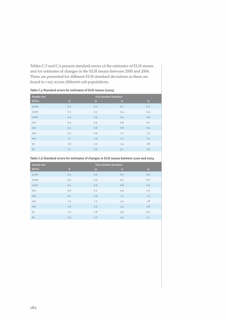
182

Tables C.5 and C.6 present standard errors of the estimates of ELSI means and for estimates of changes in the ELSI means between 2000 and 2004. These are presented for different ELSI standard deviations as these are found to vary across different sub-populations.

Table C.5 Standard errors for estimates of ELSI means (2004)

Sample size ELSI standard deviation

(EFUs) 8 10 12 14

5,000 0.2 0.2 0.2 0.3

2,000 0.3 0.3 0.4 0.4

1,000 0.4 0.4 0.5 0.6

750 0.4 0.5 0.6 0.7

500 0.5 0.6 0.8 0.9

250 0.7 0.9 1.1 1.3

100 1.1 1.4 1.7 2.0

50 1.6 2.0 2.4 2.8

30 2.1 2.6 3.1 3.6

Table C.6 Standard errors for estimates of changes in ELSI means between 2000 and 2004

Sample size ELSI standard deviation

(EFUs) 8 10 12 14

5,000 0.2 0.3 0.3 0.4

2,000 0.4 0.4 0.5 0.6

1,000 0.5 0.6 0.8 0.9

750 0.6 0.7 0.9 1.0

500 0.7 0.9 1.1 1.3

250 1.0 1.3 1.5 1.8

100 1.6 2.0 2.4 2.8

50 2.3 2.8 3.4 4.0

30 2.9 3.7 4.4 5.1

183

Appendix c

Table of confidence intervals for ELSI means presented in the report

Tables C.7 and C.8 present 95% confidence intervals and standard errors for the ELSI means found in the main figures and tables presented in this report. While the tables above give general guidelines for the standard errors of different estimates throughout the report, this table gives more precise estimates for each specific mean presented. They have been calculated using the jackknife method as outlined in Weighted Procedure for the Living Standards Survey,185 and consequently take into account the complex sampling and weighting process described above. This means that the survey estimates have wider confidence intervals compared to a simple random sample. The table also presents the “effective” sample sizes for each of the estimates. The effective sample size represents the sample size (under the assumption of simple random sampling) that would achieve the standard error that has been achieved using the complex surveying methods. This gives a further guide as to the robustness of the estimates presented.

Gray 2004. This report can be found on the web at http://www.msd.govt.nz/work-areas/social-research/living-standards/index.html.

185�

Table C.7 Confidence intervals for 2004 ELSI means of figures

Figure Category Sub-population Confidence interval Standard error

Effective sample size

Mean LCL UCL

Chapter 3: Total population

3.1 Total population 39.7 39.1 40.3 0.3 1,907

3.2 Age group Children 34.4 33.5 35.3 0.5 1,050

3.2 Age group 18–24 years 39.4 38.0 40.8 0.7 248

3.2 Age group 25–44 years 39.1 38.2 39.9 0.4 1,023

3.2 Age group 45–64 years 43.3 42.2 44.3 0.5 663

3.2 Age group 65 years or more 45.9 44.9 46.9 0.5 369

3.3 Sole parents Female 37.7 36.5 38.9 0.6 524

3.3 Sole parents Male 40.2 39.0 41.4 0.6 419

3.4 Gender Female 41.0 40.4 41.6 0.3 1,817

3.4 Gender Male 42.2 41.6 42.7 0.3 1,821

3.5 Ethnicity Mäori 32.8 31.2 34.5 0.8 294

3.5 Ethnicity Pacific 26.3 24.2 28.4 1.1 187

3.5 Ethnicity European 42.0 41.3 42.6 0.3 1,441

3.5 Ethnicity Other 39.4 37.9 40.8 0.7 290

3.6 EFU type Single with children 26.7 24.8 28.6 1.0 220

3.6 EFU type Couple with children 38.5 37.4 39.5 0.5 654

3.6 EFU type Single without children 40.7 39.8 41.7 0.5 648

3.6 EFU type Couple without children 46.3 45.7 46.9 0.3 1,023

184



Mean LCL UCL

3.7 Region Auckland 38.3 37.2 39.4 0.6 640

3.7 Region Wellington 40.2 38.2 42.2 1.0 166

3.7 Region Other major urban areas 40.3 38.9 41.7 0.7 282

3.7 Region Secondary and minor urban areas 40.0 38.6 41.5 0.7 335

3.7 Region Rural New Zealand 40.8 39.5 42.1 0.7 352

3.8 Housing tenure Rented – Housing New Zealand 21.6 19.7 23.6 1.0 200

3.8 Housing tenure Rented – private landlord 34.2 33.0 35.5 0.7 444

3.8 Housing tenure Local authority 37.9 35.8 40.0 1.1 51

3.8 Housing tenure Owned with mortgage 41.6 40.7 42.4 0.4 744

3.8 Housing tenure Owned mortgage free 47.1 46.4 47.9 0.4 609

3.8 Housing tenure Family trust 41.8 40.4 43.1 0.7 318

3.9 Qualifications No qualification 37.3 35.6 38.9 0.9 301

3.9 Qualifications School qualification 41.0 40.2 41.8 0.4 917

3.9 Qualifications Occupational certificate or diploma 41.4 40.6 42.2 0.4 940

3.9 Qualifications Bachelors degree or higher qualification 45.2 44.4 46.0 0.4 751

3.10 Occupation Elementary occupations 38.1 35.0 41.1 1.6 71

3.10 Occupation Trades, plant and machinery 38.5 36.4 40.5 1.0 146

3.10 Occupation Clerks, service and sales 39.1 36.1 42.1 1.5 71

3.10 Occupation Professionals 43.1 41.4 44.8 0.9 186


45.7 43.3 48.2 1.3 79

3.11 Employment Self-employed 46.7 45.9 47.6 0.4 498

3.11 Employment Wages and salary 42.2 41.5 42.9 0.4 1,154

3.12 Income source Income-tested benefit 25.6 23.6 27.6 1.0 198

3.12 Income source Market income 41.7 41.0 42.3 0.3 1,344

3.12 Income source New Zealand Superannuation 46.2 45.2 47.1 0.5 370

3.13 Beneficiaries Without children 32.5 30.0 34.9 1.2 120

3.13 Beneficiaries With children 21.1 19.2 23.1 1.0 164

3.14 Market income Without children 44.6 43.8 45.4 1.0 164

3.14 Market income With children 39.3 38.3 40.3 0.5 668

3.15 Equivalent disposable income $10,000 or less 29.9 28.4 31.4 0.8 359

3.15 Equivalent disposable income $10,001 – $20,000 35.7 34.9 36.6 0.4 822





3.15 Equivalent disposable income $70,001 or more 53.2 51.7 54.7 0.8 65

185

Appendix c



Mean LCL UCL

3.16 Asset value $0 – $10,000 33.7 32.9 34.6 0.5 870

3.16 Asset value $10,001 – $25,000 45.2 43.6 46.8 0.8 150

3.16 Asset value $25,001 – $100,000 45.9 45.0 46.7 0.4 369

3.16 Asset value $100,001 – $300,000 47.9 47.0 48.8 0.5 297

3.16 Asset value $300,001 – more 52.2 51.1 53.4 0.6 132

3.17 Accommodation cost Zero 42.4 40.9 43.9 0.8 251

3.17 Accommodation cost $1 – $199 per week 39.4 38.7 40.2 0.4 1,167

3.17 Accommodation cost $200 – $399 per week 37.5 36.3 38.8 0.6 446

3.17 Accommodation cost $400 or more per week 45.4 44.2 46.6 0.6 291


HOTI ≤ 15% 44.9 44.3 45.5 0.3 1,110


15% ≤ HOTI < 30% 38.7 37.6 39.9 0.6 465


30% ≤ HOTI < 45% 36.1 34.4 37.8 0.9 227


HOTI 45% or more 31.3 29.3 33.3 1.0 199

3.19 Marriage break-up None 42.7 42.1 43.4 0.3 1,380

3.19 Marriage break-up One 37.9 36.8 39.1 0.6 583

3.19 Marriage break-up Two or more 33.7 31.6 35.8 1.1 204

3.20 Life shocks None 44.2 43.3 45.1 0.5 559

3.20 Life shocks One to seven 41.8 41.2 42.4 0.3 1,792

3.20 Life shocks Eight or more 31.9 29.8 34.0 1.1 213

3.21 Health restriction None 42.2 41.7 42.7 0.3 2,030

3.21 Health restriction One or two 43.0 41.5 44.5 0.8 238

3.21 Health restriction Three or more 34.0 32.3 35.7 0.9 289

3.22 Payment difficulties None 48.0 47.6 48.4 0.2 1,338

3.22 Payment difficulties One or two 39.6 38.7 40.5 0.5 452

3.22 Payment difficulties Three to five 33.5 32.2 34.8 0.7 310

3.22 Payment difficulties Six or more 24.3 23.0 25.6 0.7 384

Chapter 4: Families with children

4.1 No children 41.6 40.8 42.5 0.4 833

4.1 With children 35.7 34.8 36.6 0.5 1,036


4.2 Income source Market income 39.5 38.5 40.5 0.5 669

4.3 Families with children Sole parents 27.1 25.2 29.0 1.0 213

4.3 Families with children Two parents 39.4 38.4 40.5 0.5 654

4.4 Sole parents Beneficiaries 22.3 20.0 24.5 1.1 130

4.4 Sole parents Market income 33.6 31.2 36.0 1.2 102

4.4 Two parents Beneficiaries 21.5 18.3 24.8 1.7 58

4.4 Two parents Market income 40.5 39.5 41.5 0.5 612

186



Mean LCL UCL

4.5 Age of mother 18–24 years 33.8 30.5 37.0 1.7 50



4.5 Age of mother 45 years or more 36.7 34.5 39.0 1.1 188

4.6 Ethnicity Mäori 31.6 29.2 34.0 1.2 166

4.6 Ethnicity Pacific 25.3 22.7 27.8 1.3 146

4.6 Ethnicity European 37.6 36.6 38.6 0.5 675

4.6 Ethnicity Other 38.4 36.4 40.4 1.0 167

4.7 Number of children One child 35.9 34.2 37.6 0.9 270

4.7 Number of children Two children 37.8 36.5 39.2 0.7 443

4.7 Number of children Three or more children 32.0 30.2 33.8 0.9 289

4.8 Age of youngest child 0–4 years 35.1 33.8 36.5 0.7 428






4.9 Housing tenure Owned 39.9 38.8 40.9 0.5 593




4.10 Qualifications Bachelors degree or higher qualification 42.5 41.2 43.7 0.6 371

4.11 Marriage break-up None 39.1 38.1 40.2 0.5 634

4.11 Marriage break-up One 33.7 32.1 35.3 0.8 303

4.11 Marriage break-up Two or more 26.5 23.9 29.1 1.3 128

4.12 GP visits Zero or one 38.1 36.0 40.2 1.1 163

4.12 GP visits Two to four 37.0 35.6 38.4 0.7 394

4.12 GP visits Five to nine 35.6 34.0 37.1 0.8 338

4.12 GP visits Ten or more 31.2 29.0 33.4 1.1 198

4.13 Restrictions – child health None 37.0 36.0 37.9 0.5 815

4.13 Restrictions – child health One or two 36.1 33.5 38.7 1.3 92

4.13 Restrictions – child health Three or more 25.6 22.5 28.8 1.6 93

4.14 Lack childcare due to cost Restricted access 24.0 22.3 25.7 0.9 237

4.14 Lack childcare due to cost All other families 37.8 36.9 38.8 0.5 833

187

Appendix c



Mean LCL UCL

Chapter 5: Older people

5.1 Older people 45.9 44.9 46.9 0.5 366

5.1 Working-age people 40.7 40.0 41.4 0.3 1,523

5.2 Age group 65–69 years 43.8 41.8 45.8 1.0 104

5.2 Age group 70–74 years 45.2 43.3 47.0 1.0 103

5.2 Age group 75–79 years 46.8 45.6 48.1 0.6 171

5.2 Age group 80 years or more 48.3 46.2 50.5 1.1 36

5.3 Sole parents Female 44.9 43.1 46.8 1.0 111

5.3 Sole parents Male 45.7 43.6 47.9 1.1 80

5.4 Older people Female 45.3 44.0 46.6 0.6 218

5.4 Older people Male 46.6 45.5 47.7 0.6 235

5.5 EFU type Single person 45.3 43.8 46.7 0.7 193

5.5 EFU type Couple only 46.6 45.5 47.7 0.6 202



5.6 Housing tenure Owned 46.7 45.7 47.7 0.5 283

5.7 Equivalent disposable income $10,000 or less 42.5 39.8 45.2 1.4 64



5.7 Equivalent disposable income $40,001 – more 51.3 47.3 55.3 2.0 12

5.8 Asset value $10,000 or less 40.1 38.4 41.9 0.9 133

5.8 Asset value $10,001 – $25,000 46.7 44.9 48.6 0.9 66

5.8 Asset value $25,001 – $100,000 47.1 45.5 48.8 0.8 82

5.8 Asset value $100,001 or more 51.8 50.4 53.2 0.7 58

5.9 Accommodation cost Nil 45.9 41.9 49.9 2.0 25

5.9 Accommodation cost $1 – $199 per week 46.1 45.2 47.0 0.5 349

5.9 Accommodation cost $200 or more per week 37.8 31.2 44.4 3.4 22

Chapter 6: Low-income population

6.1 Income distribution Bottom third 31.5 30.5 32.5 0.5 808

6.1 Income distribution Top two-thirds 43.8 43.1 44.5 0.3 1,050


6.2 Income source Market income 33.3 32.0 34.5 0.7 358

6.2 Income source New Zealand Superannuation 42.7 41.2 44.2 0.8 176

188

Table C.8 Confidence intervals for 2004 ELSI means of tables

Table Category Sub-population Confidence interval Standard error

Effective sample size Mean LCL UCL


3.1 Couple with children 18–24 years 35.2 31.5 38.9 1.9 33





3.1 Couple without children 18–24 years 39.7 37.3 42.0 1.2 73






3.1 Couple without children 75 years or more 47.8 46.6 48.9 0.6 142

3.1 Single without children 18–24 years 40.1 38.6 41.7 0.8 190






3.1 Single without children 75 years or more 47.4 45.5 49.2 1.0 70

3.1 Single with children 18–24 years 28.1 21.5 34.7 3.4 11




3.2 Females Single 37.7 36.5 38.9 0.6 524

3.2 Females Single with children 26.8 24.9 28.8 1.0 200

3.2 Females Single without children 40.5 39.2 41.8 0.7 337

3.2 Males Single 40.2 39.0 41.4 0.6 419

3.2 Males Single with children 29.6 25.4 33.8 2.1 40

3.2 Males Single without children 40.9 39.7 42.1 0.6 399

3.3 Pacific Born in New Zealand 32.5 29.9 35.1 1.3 92

3.3 Pacific Born elsewhere 28.1 25.4 30.8 1.4 136




3.4 Qualifications Bachelors degree or higher 45.2 44.4 46.0 0.4 751

189

Appendix c



3.5 Females Marriage break-up – none 42.4 41.6 43.1 0.4 1,109

3.5 Females Marriage break-up – one 36.9 35.7 38.1 0.6 538

3.5 Females Marriage break-up – two or more 32.9 30.0 35.8 1.5 113

3.5 Males Marriage break-up – none 44.0 43.2 44.7 0.4 795

3.5 Males Marriage break-up – one 41.6 40.0 43.2 0.8 246

3.5 Males Marriage break-up – two or more 37.0 34.1 39.8 1.5 103


4.1 Total population All families – income-tested benefit 28.4 26.3 30.4 1.0 182

4.1 Total population All families – market income 42.5 41.8 43.1 0.3 1,337

4.1 Total population Couple only – income-tested benefit 34.3 29.6 39.0 2.4 23

4.1 Total population Couple only – market income 46.9 46.2 47.6 0.4 770

4.1 Total population Couple with children – income-tested benefit

21.5 18.3 24.8 1.7 58

4.1 Total population Couple with children – market income 40.4 39.4 41.4 0.5 612

4.1 Total population One-parent family – income-tested benefit

22.3 20.0 24.5 1.1 130

4.1 Total population One-parent family – market income 33.6 31.2 36.0 1.2 102

4.1 Total population Single person – income-tested benefit 31.5 28.7 34.3 1.4 94

4.1 Total population Single person – market income 42.1 41.0 43.2 0.6 386

4.1 Mäori All families – income-tested benefit 26.1 21.6 30.6 2.3 38

4.1 Mäori All families – market income 38.2 36.3 40.2 1.0 173

4.1 Mäori Couple only – income-tested benefit 19.9 2.8 37.0 8.7 2

4.1 Mäori Couple only – market income 41.0 37.8 44.2 1.6 51

4.1 Mäori Couple with children – income-tested benefit

21.2 13.7 28.6 3.8 11

4.1 Mäori Couple with children – market income 37.2 34.3 40.1 1.5 93

4.1 Mäori One-parent family – income-tested benefit

23.0 17.3 28.6 2.9 27

4.1 Mäori One-parent family – market income 31.7 25.3 38.2 3.3 16

4.1 Mäori Single person – income-tested benefit 30.4 24.7 36.1 2.9 18

4.1 Mäori Single person – market income 38.8 35.6 42.0 1.6 59

4.1 Pacific All families – income-tested benefit 18.7 15.8 21.6 1.5 52

4.1 Pacific All families – market income 31.2 28.5 33.9 1.4 114

4.1 Pacific Couple with children – income-tested benefit

8.7 5.0 12.3 1.9 12

4.1 Pacific Couple with children – market income 28.3 24.9 31.7 1.7 88

4.1 Pacific One-parent family – income-tested benefit

17.0 12.9 21.1 2.1 38

4.1 Pacific One-parent family – market income 30.0 23.7 36.4 3.2 10

190



4.4 GP visit – none to one Families – one child 37.7 34.1 41.3 1.8 55

4.4 GP visit – none to one Families – two children 41.5 39.0 43.9 1.2 101

4.4 GP visit – none to one Families – three or more children 31.8 26.5 37.2 2.7 32

4.4 GP visit – two to four Families – one child 36.7 34.5 38.9 1.1 150

4.4 GP visit – two to four Families – two children 38.6 36.6 40.6 1.0 201

4.4 GP visit – two to four Families – three or more children 35.2 31.8 38.5 1.7 86

4.4 GP visit – five to nine Families – one child 35.5 32.6 38.3 1.4 92

4.4 GP visit – five to nine Families – two children 37.5 34.9 40.1 1.3 121

4.4 GP visit – five to nine Families – three or more children 32.6 29.5 35.6 1.5 89

4.4 GP visit – ten or more Families – one child 27.5 19.8 35.2 3.9 16

4.4 GP visit – ten or more Families – two children 34.2 31.0 37.5 1.6 78

4.4 GP visit – ten or more Families – three or more children 29.7 26.7 32.8 1.6 107

4.5 Restrictions – none Families – one child 37.0 35.5 38.5 0.8 311

4.5 Restrictions – none Families – two children 39.0 37.5 40.6 0.8 312

4.5 Restrictions – none Families – three or more children 33.4 31.3 35.5 1.1 205

4.5 Restrictions – one or two Families – one child 35.3 29.8 40.9 2.8 20

4.5 Restrictions – one or two Families – two children 36.0 30.9 41.1 2.6 30

4.5 Restrictions – one or two Families – three or more children 37.0 32.4 41.5 2.3 26

4.5 Restrictions – three or more Families – one child 22.3 13.6 31.0 4.4 14

4.5 Restrictions – three or more Families – two children 29.8 26.5 33.2 1.7 67

4.5 Restrictions – three or more Families – three or more children 23.2 18.7 27.6 2.3 44

Chapter 5: Older New Zealanders

5.2 New Zealand Superannuation type

Couple, both qualify 46.1 45.0 47.3 0.6 208


Couple, one qualify 47.8 44.2 51.5 1.8 23


Single, living alone 45.9 44.5 47.4 0.7 171


Single, sharing 45.6 42.8 48.5 1.5 38

191

Appendix c

Table C.9 presents estimates of differences between the 2000 and 2004 ESLI means, standard errors for these differences and associated t-statistics and p-values. The standard errors have been calculated using the jackknife method for both 2000 and 2004 and consequently reflect the complex sampling and weighting processes used in producing the estimates. The t-statistics and p-values enable us to determine the statistical significance of the changes between the two years. Where the p-value is less than 0.05, an asterisk is printed next to the estimate, indicating it is significant at the 95% confidence level.

Table C.9 Statistical significance of differences in ELSI means between 2000 and 2004

Figure Category Sub-population Mean 2004

Mean 2000

Difference in means

2004 – 2000

Standard error of

difference

t-value p-value Level of signifi-cance


3.1 Total population 39.7 40.6 –1.0 0.4 –2.23 0.03 *

3.2 Age group Children 34.4 36.4 –1.9 0.6 –3.33 0.00 *

3.2 Age group 18–24 years 39.4 41.2 –1.8 0.9 –1.96 0.05

3.2 Age group 25–44 years 39.1 39.9 –0.8 0.6 –1.36 0.18

3.2 Age group 45–64 years 43.3 43.2 0.0 0.7 0.04 0.97

3.2 Age group 65 years or more 45.9 47.4 –1.5 0.5 –2.81 0.01 *

3.3 Sole parents Female 37.7 39.6 –1.9 0.8 –2.25 0.02 *

3.3 Sole parents Male 40.2 42.2 –2.0 0.9 –2.26 0.02 *

3.4 Gender Female 41.0 41.6 –0.6 0.5 –1.34 0.18

3.4 Gender Male 42.2 42.8 –0.6 0.5 –1.31 0.19

3.5 Ethnicity Mäori 32.8 34.4 –1.6 1.1 –1.49 0.14

3.5 Ethnicity Pacific 26.3 29.8 –3.4 1.8 –1.93 0.06

3.5 Ethnicity European 42.0 42.9 –0.9 0.5 –1.97 0.05 *

3.5 Ethnicity Other 39.4 38.0 1.3 1.3 1.02 0.31

3.6 EFU type Single with children 26.7 28.8 –2.1 1.2 –1.79 0.07

3.6 EFU type Couple with children 38.5 39.4 –1.0 0.7 –1.40 0.16

3.6 EFU type Single without children 40.7 42.5 –1.8 0.7 –2.60 0.01 *

3.6 EFU type Couple without children 46.3 45.5 0.8 0.6 1.40 0.16

3.7 Region Auckland 38.3 39.2 –0.9 0.9 –0.97 0.33

3.7 Region Wellington 40.2 42.6 –2.4 1.3 –1.87 0.06

3.7 Region Other major urban areas 40.3 40.4 –0.1 0.9 –0.07 0.95


40.0 41.0 –1.0 1.1 –0.84 0.40

3.7 Region Rural New Zealand 40.8 42.4 –1.6 0.9 –1.80 0.07

192


Mean 2000

Difference in means

2004 – 2000

Standard error of

difference



21.6 25.4 –3.7 1.6 –2.31 0.02 *

3.8 Housing tenure Rented – private landlord 34.2 34.9 –0.7 0.9 –0.79 0.43

3.8 Housing tenure Local authority 37.9 34.7 3.2 3.0 1.08 0.29

3.8 Housing tenure Owned with mortgage 41.6 41.8 –0.2 0.6 –0.30 0.77

3.8 Housing tenure Owned mortgage free 47.1 47.5 –0.4 0.8 –0.49 0.62

3.8 Housing tenure Family trust 41.8 42.9 –1.2 0.8 –1.40 0.16

3.9 Qualifications No qualification 37.3 39.6 –2.4 1.1 –2.21 0.03 *

3.9 Qualifications School qualification 41.0 42.3 –1.3 0.7 –1.97 0.05 *


41.4 42.0 –0.6 0.6 –1.05 0.30

3.9 Qualifications Bachelors degree or higher

45.2 45.9 –0.8 0.7 –1.04 0.30

3.10 Occupation Elementary occupations 38.1 42.2 –4.1 1.8 –2.23 0.03 *

3.10 Occupation Trades, plant and machinery

38.5 38.9 –0.5 1.4 –0.31 0.75

3.10 Occupation Clerks, service and sales 39.1 41.0 –1.9 1.9 –1.02 0.31

3.10 Occupation Professionals 43.1 45.9 –2.8 1.2 –2.24 0.03 *


45.7 46.2 –0.5 1.7 –0.28 0.78

3.11 Employment Self-employed 45.4 44.3 1.1 1.3 0.82 0.42

3.11 Employment Wages and salary 40.3 42.0 –1.7 0.8 –2.09 0.04 *

3.12 Source of income Income-tested benefit 25.6 28.7 –3.1 1.2 –2.53 0.01 *

3.12 Source of income Market income 41.7 42.3 –0.6 0.5 –1.33 0.18

3.12 Source of income New Zealand Superannuation

46.2 47.2 –1.0 1.0 –0.97 0.33

3.13 Beneficiaries Without children 32.5 33.5 –1.0 1.6 –0.7 0.5

3.13 Beneficiaries With children 21.1 25.3 –4.2 1.3 –3.3 0.0 *

3.14 Market income Without children 44.6 45.0 –0.4 0.6 –0.7 0.5

3.14 Market income With children 39.3 40.1 –0.8 0.6 –1.2 0.2

3.15 Equivalent disposable income

$10,000 or less 29.9 30.2 –0.3 1.1 –0.27 0.79


$10,001 – $20,000 35.7 38.5 –2.8 0.7 –3.95 0.00 *


$20,001 – $30,000 41.4 43.3 –1.9 0.8 –2.27 0.02 *


$30,001 – $40,000 45.8 47.7 –1.9 0.7 –2.70 0.01 *


$40,001 – $50,000 48.4 51.6 –3.2 1.5 –2.13 0.04 *


$50,001 – $70,000 52.0 53.2 –1.2 0.8 –1.48 0.14


$70,001 or more 53.2 54.8 –1.6 1.5 –1.04 0.30

193

Appendix c


Mean 2000

Difference in means

2004 – 2000

Standard error of

difference


3.16 Asset value $10,000 or less 33.7 36.9 –3.2 0.6 –5.06 0.00 *

3.16 Asset value $10,001 – $25,000 45.2 44.6 0.6 1.1 0.58 0.56

3.16 Asset value $25,001 – $100,000 45.9 45.2 0.7 0.9 0.77 0.44

3.16 Asset value $100,001 – $300,000 47.9 46.7 1.2 0.7 1.68 0.09

3.16 Asset value $300,001 or more 52.2 51.3 1.0 0.7 1.30 0.20

3.17 Accommodation cost Zero 42.4 47.0 –4.6 0.9 –5.01 0.00 *

3.17 Accommodation cost $1 – $199 per week 39.4 36.6 2.8 0.6 4.74 0.00 *

3.17 Accommodation cost $200 – $399 per week 37.5 37.5 0.0 0.9 0.06 0.96

3.17 Accommodation cost $400 or more per week 45.4 47.1 –1.7 1.1 –1.48 0.14


HOTI ≤ 15% 44.9 46.6 –1.7 0.5 –3.27 0.00 *


15% ≤ HOTI < 30% 38.7 42.0 –3.3 0.8 –4.35 0.00 *


30% ≤ HOTI < 45% 36.1 35.6 0.5 1.2 0.40 0.69


HOTI 45% or more 31.3 30.2 1.1 1.3 0.89 0.38


4.1 No children 41.6 42.5 –0.9 0.6 –1.52 0.13

4.1 With children 35.7 36.9 –1.1 0.6 –1.92 0.05

4.2 Income source Income–tested benefit 22.2 26.2 –4.1 1.3 –3.18 0.00 *

4.2 Income source Market income 39.5 40.2 –0.7 0.6 –1.05 0.29

4.3 Families with children Sole parents 27.1 29.6 –2.4 1.2 –2.04 0.04 *

4.3 Families with children Two parents 39.4 39.8 –0.4 0.7 –0.58 0.56

4.4 Sole parents Beneficiaries 22.3 26.5 –4.2 1.4 –2.94 0.00 *

4.4 Sole parents Market income 33.6 35.5 –1.9 1.8 –1.08 0.28

4.4 Two parents Beneficiaries 21.5 25.0 –3.5 2.3 –1.54 0.13

4.4 Two parents Market income 40.5 40.9 –0.4 0.7 –0.59 0.55

4.5 Age of mother 18–24 years 33.8 32.8 0.9 2.2 0.42 0.68

4.5 Age of mother 25–34 years 34.2 34.9 –0.7 1.1 –0.66 0.51


4.5 Age of mother 45 years or more 36.7 40.8 –4.1 1.6 –2.60 0.01 *

4.6 Ethnicity Mäori 31.6 31.7 –0.1 1.5 –0.08 0.94

4.6 Ethnicity Pacific 25.3 28.8 –3.5 2.0 –1.78 0.08

4.6 Ethnicity European 37.6 39.3 –1.6 0.7 –2.41 0.02 *

4.6 Ethnicity Other 38.4 35.8 2.6 1.6 1.66 0.10

4.7 Number of children One child 35.9 37.1 –1.2 1.1 –1.11 0.27

4.7 Number of children Two children 37.8 37.6 0.2 0.9 0.21 0.83

4.7 Number of children Three or more children 32.0 35.2 –3.2 1.2 –2.71 0.01 *

194


Mean 2000

Difference in means

2004 – 2000

Standard error of

difference


4.8 Age of youngest child 0–4 years 35.1 35.7 –0.6 0.9 –0.66 0.51





19.9 25.0 –5.0 2.0 –2.56 0.01 *

4.9 Housing tenure Rented – private landlord 30.5 30.2 0.3 1.1 0.28 0.78

4.9 Housing tenure Owned 39.9 40.8 –1.0 0.7 –1.42 0.16

4.10 Qualifications No qualification 27.1 29.8 –2.7 1.7 –1.59 0.11

4.10 Qualifications School qualification 33.9 36.5 –2.6 1.0 –2.64 0.01 *


36.0 38.1 –2.0 1.0 –2.10 0.04 *

4.10 Qualifications Bachelors degree or higher qualification

42.5 43.0 –0.5 1.1 –0.51 0.61


5.1 Older people 45.9 47.4 –1.5 0.5 –2.77 0.01 *

5.1 Working-age people 40.7 41.2 –0.5 0.4 –1.23 0.22

5.2 Age group 65–69 years 43.8 46.0 –2.2 1.1 –2.00 0.05 *

5.2 Age group 70–74 years 45.2 46.8 –1.6 1.0 –1.57 0.12

5.2 Age group 75–79 years 46.8 48.1 –1.3 0.8 –1.68 0.10

5.2 Age group 80 years or more 48.3 49.7 –1.3 1.1 –1.17 0.25

5.3 Sole parents Female 44.9 46.8 –1.8 1.0 –1.78 0.08

5.3 Sole parents Male 45.7 47.2 –1.5 1.2 –1.21 0.23

5.4 Older people Female 45.3 47.4 –2.1 0.7 –2.91 0.00 *

5.4 Older people Male 46.6 47.5 –0.9 0.6 –1.43 0.15

5.5 EFU type Single person 45.3 46.9 –1.7 0.8 –2.15 0.03 *

5.5 EFU type Couple only 46.6 47.9 –1.3 0.6 –2.05 0.04 *


34.0 36.8 –2.9 2.9 –0.98 0.34


5.6 Housing tenure Owned 46.7 48.0 –1.3 0.5 –2.43 0.02 *


$10,000 or less 42.5 43.5 –1.0 2.1 –0.48 0.63


$10,001 – $20,000 44.0 46.0 –2.0 0.6 –3.18 0.00 *


$20,001 – $40,000 49.6 51.0 –1.4 0.9 –1.49 0.14


$40,001 or more 51.3 55.4 –4.1 2.1 –1.97 0.07

195

Appendix c


Mean 2000

Difference in means

2004 – 2000

Standard error of

difference


5.8 Asset value $10,000 or less 40.1 43.3 –3.2 1.0 –3.28 0.00 *

5.8 Asset value $10,001 – $25,000 46.7 47.6 –0.9 1.1 –0.81 0.42

5.8 Asset value $25,001 – $100,000 47.1 49.3 –2.1 0.9 –2.36 0.02 *

5.8 Asset value $100,001 or more 51.8 52.5 –0.7 0.8 –0.88 0.38

5.9 Accommodation cost Zero 45.9 48.6 –2.6 2.0 –1.29 0.21


5.9 Accommodation cost $200 or more 37.8 41.5 –3.6 4.0 –0.92 0.37

Chapter 6: Low–income population

6.1 Income distribution Bottom third 31.5 34.1 –2.6 0.7 –3.53 0.00 *

6.1 Income distribution Top two-thirds 43.8 44.9 –1.1 0.5 –2.23 0.03 *

6.2 Income source Income-tested benefit 24.3 28.2 –3.9 1.3 –2.95 0.00 *

6.2 Income source Market income 33.3 34.9 –1.6 1.0 –1.61 0.11


42.7 44.9 –2.2 1.5 –1.53 0.13

196

Table C.10 presents estimates of differences in proportions in hardship (ELSI levels 1 to 3) between 2000 and 2004, standard errors for these differences and associated t-statistics and p-values. The standard errors have been calculated using the same method as with table C.9. The t-statistics and p-values enable us to determine the statistical significance of the changes between the two years. Where the p-value is less than 0.05, an asterisk is printed next to the estimate, indicating it is significant at the 95% confidence level.

Table C.10 Statistical significance of differences in hardship (ELSI levels 1 to 3) between 2000 and 2004

Figure Category Sub-population Estimate of % in

hardship 2004

Estimate of % in

hardship 2000

Difference 2004

– 2000

Standard error of

difference



3.1 Total population Population 24.0 23.6 0.4 1.5 0.27 0.79

3.2 Age group Children 37.7 35.8 1.9 1.8 1.03 0.30

3.2 Age group 18–24 years 22.1 18.8 3.3 3.7 0.89 0.38

3.2 Age group 25–44 years 24.2 24.9 –0.7 2.0 –0.36 0.72

3.2 Age group 45–64 years 17.1 17.8 –0.7 2.1 –0.34 0.74

3.2 Age group 65 years or more 8.2 6.5 1.6 1.9 0.87 0.38

3.3 Sole parents Female 29.9 25.7 4.1 3.1 1.35 0.18

3.3 Sole parents Male 18.7 18.2 0.5 2.9 0.18 0.86

3.4 Gender Female 21.5 20.8 0.7 1.6 0.42 0.67

3.4 Gender Male 16.6 17.6 –1.0 1.4 –0.72 0.47

3.5 Ethnicity Mäori 40.4 41.1 –0.7 3.8 –0.19 0.85

3.5 Ethnicity Pacific 57.9 56.5 1.4 6.4 0.22 0.83

3.5 Ethnicity European 18.8 17.2 1.6 1.5 1.05 0.29

3.5 Ethnicity Other 23.5 28.9 –5.4 4.4 –1.25 0.21

3.6 EFU type Single with children 61.1 57.3 3.8 4.4 0.86 0.39

3.6 EFU type Couple with children 25.6 26.4 –0.8 2.0 –0.41 0.68

3.6 EFU type Single without children 19.3 17.4 1.9 2.4 0.77 0.44

3.6 EFU type Couple without children 9.5 11.5 –2.0 1.6 –1.22 0.22

3.7 Region Auckland 28.4 29.1 –0.7 2.9 –0.24 0.81

3.7 Region Wellington 24.7 16.5 8.2 4.6 1.79 0.08

3.7 Region Other major urban areas 21.2 23.6 –2.4 3.1 –0.78 0.44


22.7 22.2 0.5 3.4 0.14 0.89

3.7 Region Rural New Zealand 20.6 19.0 1.7 2.9 0.58 0.56

197

Appendix c


hardship 2004

Estimate of % in

hardship 2000

Difference 2004

– 2000

Standard error of

difference



71.8 70.9 0.9 6.4 0.14 0.89


3.8 Housing tenure Local authority 20.0 46.5 –26.5 11.0 –2.39 0.02 *

3.8 Housing tenure Owned with mortgage 17.5 18.9 –1.4 1.9 –0.72 0.47


3.8 Housing tenure Family trust 18.0 17.2 0.8 2.7 0.31 0.76

3.9 Qualifications No qualification 28.8 25.5 3.3 3.1 1.05 0.30

3.9 Qualifications School qualification 19.8 18.5 1.4 2.2 0.62 0.53


20.0 19.6 0.5 2.0 0.24 0.81


10.8 11.0 –0.3 1.9 –0.14 0.89

3.10 Main occupation Elementary occupations 18.7 16.6 2.1 5.2 0.40 0.69

3.10 Main occupation Trades, plant and machine

26.2 27.2 –1.0 4.7 –0.21 0.83

3.10 Main occupation Clerks, service and sales 27.0 22.3 4.7 6.7 0.71 0.48

3.10 Main occupation Professionals 17.4 10.1 7.3 3.7 1.94 0.05

3.10 Main occupation Legislators, administrators and managers

9.3 9.4 –0.1 4.4 –0.01 0.99

3.11 Employment Self-employed 5.5 13.3 –7.7 2.9 –2.70 0.01 *

3.11 Employment Wages and salary 22.7 19.4 3.3 2.7 1.22 0.22

3.12 Source of income Income-tested benefit 60.5 56.0 4.5 4.7 0.96 0.34

3.12 Source of income Market income 18.9 18.9 0.0 1.4 –0.02 0.98


7.9 7.1 0.7 3.8 0.19 0.85

3.13 Beneficiaries Without children 39.1 38.2 0.9 6.1 0.14 0.89

3.13 Beneficiaries With children 74.4 68.7 5.8 4.9 1.18 0.24

3.14 Market incomes Without children 12.5 12.4 0.1 1.8 0.06 0.95

3.14 Market incomes With children 24.0 24.2 –0.2 2.0 –0.10 0.92


$10,000 or less 49.8 51.1 –1.3 3.8 –0.35 0.73


$10,001 – $20,000 31.4 28.0 3.5 2.5 1.38 0.17


$20,001 – $30,000 18.5 14.5 4.0 2.8 1.42 0.16


$30,001 – $40,000 7.3 3.8 3.5 1.6 2.22 0.03 *


$40,001 – $50,000 4.7 2.3 2.4 2.8 0.86 0.39


$50,001 – $70,000 2.7 0.4 2.3 1.9 1.17 0.25


$70,001 or more 0.1 0.0 0.1 0.2 0.73 0.47

198


hardship 2004

Estimate of % in

hardship 2000

Difference 2004

– 2000

Standard error of

difference


3.16 Asset value $10,000 or less 38.0 32.4 5.6 2.4 2.34 0.02 *

3.16 Asset value $10,001 – $25,000 7.3 10.4 –3.1 2.8 –1.09 0.28

3.16 Asset value $25,001 – $100,000 9.0 10.3 –1.2 1.8 –0.71 0.48

3.16 Asset value $100,001 – $300,000 4.9 6.9 –2.1 1.7 –1.22 0.22


3.17 Accommodation cost Zero 15.9 8.3 7.6 2.8 2.75 0.01 *

3.17 Accommodation cost $1 – $199 per week 24.6 32.8 –8.2 2.0 –4.02 0.00 *

3.17 Accommodation cost $200 – $399 per week 29.5 32.3 –2.8 2.9 –0.97 0.33

3.17 Accommodation cost $400 or more per week 11.0 5.2 5.7 2.3 2.46 0.02 *


HOTI ≤ 15% 11.7 8.2 3.5 1.4 2.51 0.01 *


15% ≤ HOTI < 30% 24.2 19.2 5.1 2.5 2.05 0.04 *


30% ≤ HOTI < 45% 34.3 35.7 –1.4 4.6 –0.31 0.76


HOTI 45% or more 45.9 51.5 –5.6 4.4 –1.28 0.20


4.1 Families No children 18.2 17.7 0.5 2.0 0.26 0.80

4.1 Families With children 33.9 33.4 0.5 1.8 0.25 0.80

4.2 Income source Income-tested benefit 72.2 65.5 6.6 4.9 1.36 0.18

4.2 Income source Market income 23.5 23.4 0.1 2.0 0.04 0.97

4.3 Families with children Sole parents 59.6 55.0 4.5 4.4 1.04 0.30

4.3 Families with children Two parents 22.9 24.6 –1.8 2.0 –0.87 0.38

4.4 Sole parents Beneficiaries 71.5 64.0 7.5 5.5 1.36 0.18

4.4 Sole parents Market income 45.5 37.4 8.1 6.9 1.17 0.24

4.4 Two parents Beneficiaries 75.5 72.0 3.5 8.7 0.41 0.69

4.4 Two parents Market income 19.9 21.4 –1.5 2.0 –0.73 0.47




4.5 Age of mother 45 years or more 33.2 23.8 9.4 4.8 1.96 0.05

4.6 Ethnicity Mäori 44.1 49.5 –5.4 5.4 –1.00 0.32

4.6 Ethnicity Pacific 60.7 58.8 1.9 7.0 0.28 0.78


4.6 Ethnicity Other 26.8 34.5 –7.8 6.0 –1.29 0.20

4.7 Number of children One child 31.9 31.3 0.6 3.6 0.17 0.87

4.7 Number of children Two children 30.3 30.5 –0.2 2.9 –0.06 0.95

4.7 Number of children Three or more children 43.3 41.7 1.7 4.1 0.40 0.69

199

Appendix c


hardship 2004

Estimate of % in

hardship 2000

Difference 2004

– 2000

Standard error of

difference



4.8 Age of youngest child 5–9 years 37.4 37.4 0.1 3.8 0.01 0.99




76.7 73.2 3.5 6.2 0.56 0.58


4.9 Housing tenure Owned 22.4 21.8 0.6 2.1 0.28 0.78

4.10 Qualifications No qualification 56.0 53.5 2.5 5.8 0.44 0.66

4.10 Qualifications School qualification 40.3 33.5 6.8 3.4 2.01 0.04 *


32.6 29.3 3.3 3.2 1.03 0.30


15.7 19.6 –3.9 3.4 –1.15 0.25


5.1 Older people Older population 8.1 6.5 1.5 1.9 0.82 0.41

5.1 Working-age people Working age 21.2 21.6 –0.3 1.5 –0.23 0.82

5.2 Age group 65–69 years 11.2 8.8 2.4 3.4 0.70 0.49

5.2 Age group 70–74 years 10.4 8.7 1.7 3.1 0.56 0.57

5.2 Age group 75–79 years 4.7 4.5 0.2 1.8 0.12 0.90




5.4 Older people Female 9.2 6.3 2.9 2.2 1.30 0.20

5.4 Older people Male 6.1 6.8 –0.6 1.9 –0.34 0.73

5.5 Family type Couple only 5.1 5.8 –0.6 1.7 –0.37 0.71

5.5 Family type Single person 10.5 7.1 3.4 2.7 1.26 0.21


40.9 30.8 10.1 12.1 0.84 0.41




$10,000 or less 14.3 11.0 3.3 6.4 0.52 0.61


$10,001 – $20,000 9.0 8.0 1.0 1.9 0.52 0.60


$20,001 – $40,000 5.7 1.5 4.2 3.0 1.42 0.16


$40,001 or more 2.0 0.0 2.0 4.9 0.41 0.69

200


hardship 2004

Estimate of % in

hardship 2000

Difference 2004

– 2000

Standard error of

difference


5.8 Asset value $10,000 or less 19.1 13.2 6.0 4.0 1.50 0.14

5.8 Asset value $10,001 – $25,000 4.2 4.9 –0.7 2.7 –0.27 0.79

5.8 Asset value $25,001 – $100,000 3.3 1.7 1.6 1.9 0.87 0.39


5.9 Accommodation cost Zero 8.5 4.3 4.2 5.9 0.72 0.48


5.9 Accommodation cost $200 or more per week 33.8 22.3 11.5 12.3 0.93 0.36


6.1 High income Top two-thirds 13.6 12.7 0.9 1.5 0.61 0.54

6.1 Low income Bottom third 44.9 40.1 4.8 2.7 1.78 0.08

6.2 Income source Income-tested benefit 65.0 58.0 6.9 4.6 1.50 0.14



13.4 9.4 3.9 5.8 0.68 0.50

201

Appendix c

Table C.11 presents estimates of differences in proportions in “severe hardship” (ELSI level 1) between 2000 and 2004, standard errors for these differences and associated t-statistics and p-values. The standard errors have been calculated using the same method as with table C.9. The t-statistics and p-values enable us to determine the statistical significance of the changes between the two years. Where the p-value is less than 0.05, an asterisk is printed next to the estimate, indicating it is significant at the 95% confidence level.

Note that results in chapter 5 from figure 5.2 onwards are for changes in levels 1 and 2 “severe” and “significant hardship”.

Table C.11 Statistical significance of differences in “severe hardship” (ELSI level 1) between 2000 and 2004

Figure Category Sub-population Estimate of % in severe

hardship 2004

Estimate of % in severe

hardship 2000

Difference 2004

– 2000

Standard error of

difference



3.1 Total population Population 7.6 4.7 2.9 0.7 4.23 0.00 *

3.2 Age group Children 14.1 7.9 6.1 1.3 4.72 0.00 *

3.2 Age group 18–24 years 3.1 2.3 0.8 1.3 0.64 0.52

3.2 Age group 25–44 years 7.9 4.6 3.3 1.1 3.03 0.00 *

3.2 Age group 45–64 years 4.9 4.0 1.0 1.3 0.74 0.46



3.3 Sole parents Male 5.5 2.5 3.1 1.3 2.39 0.02 *

3.4 Gender Female 6.0 4.2 1.8 0.8 2.24 0.03 *

3.4 Gender Male 4.4 2.7 1.7 0.7 2.49 0.01 *

3.5 Ethnicity Mäori 16.9 7.5 9.4 2.4 3.88 0.00 *

3.5 Ethnicity Pacific 27.3 15.2 12.1 3.9 3.13 0.00 *


3.5 Ethnicity Other 5.8 6.2 –0.4 2.1 –0.18 0.86

3.6 EFU type Single with children 22.0 17.1 4.9 3.3 1.50 0.13

3.6 EFU type Couple with children 8.8 4.5 4.4 1.2 3.62 0.00 *

3.6 EFU type Single without children 5.3 2.7 2.6 1.1 2.46 0.01 *

3.6 EFU type Couple without children 1.4 1.8 –0.4 0.8 –0.48 0.63

3.7 Region Auckland 10.2 5.2 5.0 1.2 4.24 0.00 *

3.7 Region Wellington 5.6 2.5 3.1 2.3 1.34 0.18

3.7 Region Other major urban areas 6.1 5.4 0.8 1.4 0.54 0.59


7.2 4.4 2.8 1.8 1.58 0.12

3.7 Region Rural New Zealand 6.7 3.8 2.9 1.4 2.12 0.03 *

202


hardship 2004


hardship 2000

Difference 2004

– 2000

Standard error of

difference



38.5 19.5 19.1 4.9 3.93 0.00 *

3.8 Housing tenure Rented – private landlord 12.4 8.0 4.3 1.7 2.55 0.01 *

3.8 Housing tenure Local authority 1.7 6.5 –4.8 11.0 –0.43 0.66

3.8 Housing tenure Owned with mortgage 3.9 3.6 0.3 1.1 0.31 0.76


3.8 Housing tenure Family trust 4.4 2.0 2.3 1.1 2.01 0.05 *

3.9 Qualifications No qualification 11.8 5.8 6.0 2.2 2.70 0.01 *

3.9 Qualifications School qualification 5.2 3.9 1.3 1.1 1.20 0.23


4.6 2.5 2.1 0.8 2.53 0.01 *


1.7 1.6 0.1 0.7 0.17 0.86

3.10 Main occupation Elementary occupations 10.8 2.4 8.4 2.9 2.90 0.00 *

3.10 Main occupation Trades, plant and machine

5.4 4.6 0.8 1.8 0.44 0.66

3.10 Main occupation Clerks, service and sales 7.6 2.2 5.4 3.4 1.56 0.12

3.10 Main occupation Professionals 2.8 0.4 2.5 0.9 2.79 0.01 *

3.10 Main occupation Legislators, administrators and managers

2.5 0.3 2.1 2.1 1.02 0.31

3.11 Employment Self-employed 1.8 0.6 1.3 1.5 0.88 0.38

3.11 Employment Wages and salary 5.3 2.7 2.6 1.3 2.10 0.04 *

3.12 Source of income Income-tested benefit 26.1 16.7 9.4 2.8 3.33 0.00 *

3.12 Source of income Market income 4.5 2.6 1.9 0.6 2.94 0.00 *


1.0 0.8 0.2 1.3 0.17 0.86

3.13 Beneficiaries Without children 13.7 10.1 3.6 3.4 1.05 0.30

3.13 Beneficiaries With children 34.2 21.4 12.8 4.3 2.99 0.00 *

3.14 Market income Without children 2.3 1.1 1.2 0.7 1.60 0.11

3.14 Market income With children 6.2 3.7 2.5 1.1 2.31 0.02 *


$10,000 or less 21.5 16.0 5.6 2.4 2.34 0.02 *


$10,001 – $20,000 8.1 4.0 4.1 1.3 3.23 0.00 *


$20,001 – $30,000 3.4 1.5 1.9 1.5 1.24 0.22


$30,001 – $40,000 0.4 0.1 0.3 0.3 1.37 0.17


$40,001 – $50,000 0.0 0.0 0.0 0.0 – –


$50,001 – $70,000 0.4 0.0 0.4 0.3 1.32 0.20


$70,001 or more 0.0 0.0 0.0 0.0 – –

203

Appendix c


hardship 2004


hardship 2000

Difference 2004

– 2000

Standard error of

difference



3.16 Asset value $10,001 – $25,000 0.9 0.5 0.4 1.5 0.29 0.77

3.16 Asset value $25,001 – $100,000 1.4 2.1 –0.6 0.6 –0.96 0.34

3.16 Asset value $100,001 – $300,000 0.5 0.7 –0.2 0.3 –0.65 0.52


3.17 Accommodation cost Zero 4.4 0.8 3.6 1.7 2.10 0.04 *


3.17 Accommodation cost $200 – $399 per week 7.5 7.5 0.0 1.6 0.00 1.00

3.17 Accommodation cost $400 or more per week 1.8 0.0 1.8 0.7 2.70 0.07 *


HOTI ≤ 15% 2.8 0.9 2.0 0.7 2.95 0.00 *


15% ≤ HOTI < 30% 7.3 1.3 6.0 1.1 5.42 0.00 *


30% ≤ HOTI < 45% 9.3 6.5 2.8 2.5 1.12 0.26


HOTI 45% or more 15.6 16.0 –0.4 2.5 –0.14 0.89


4.1 Families No children 4.8 2.8 2.0 0.9 2.27 0.02 *

4.1 Families With children 11.2 7.7 3.5 1.3 2.68 0.01 *

4.2 Income source Income-tested benefit 31.6 20.4 11.2 4.3 2.61 0.01 *


4.3 Families with children Sole parents 21.0 16.1 4.9 3.3 1.49 0.14

4.3 Families with children Two parents 7.0 4.3 2.7 1.2 2.23 0.03 *

4.4 Sole parents Beneficiaries 31.7 20.9 10.9 4.8 2.24 0.03 *

4.4 Sole parents Market income 5.6 6.8 –1.2 3.4 –0.35 0.72

4.4 Two parents Beneficiaries 30.9 18.3 12.6 8.5 1.49 0.14

4.4 Two parents Market income 5.4 3.4 2.0 1.1 1.79 0.07


4.5 Age of mother 25–34 years 14.6 8.8 5.8 2.5 2.32 0.02 *


4.5 Age of mother 45 years or more 10.9 5.0 5.9 3.2 1.84 0.07

4.6 Ethnicity Mäori 20.0 10.7 9.3 4.1 2.28 0.02 *

4.6 Ethnicity Pacific 30.2 16.0 14.2 5.7 2.47 0.02 *


4.6 Ethnicity Other 4.4 7.2 –2.9 3.0 –0.97 0.34

4.7 Number of children One child 10.4 7.8 2.7 2.5 1.07 0.28

4.7 Number of children Two children 7.5 7.6 -0.1 1.6 -0.09 0.93

4.7 Number of children Three or more children 18.7 7.8 10.9 2.5 4.37 0.00 *

204


hardship 2004


hardship 2000

Difference 2004

– 2000

Standard error of

difference



4.8 Age of youngest child 5–9 years 13.5 8.1 5.5 2.7 2.05 0.04 *




41.0 18.7 22.4 6.5 3.44 0.00 *



4.10 Qualifications No qualification 26.9 14.2 12.7 4.6 2.75 0.01 *

4.10 Qualifications School qualification 12.6 7.8 4.8 2.3 2.07 0.04 *


9.5 6.1 3.4 2.0 1.71 0.09


2.7 3.6 –0.9 1.3 –0.69 0.49

Chapter 5: Older people186

5.1 Older people Older population 1.1 0.7 0.4 0.7 0.51 0.61

5.1 Working-age people Working age 6.0 4.0 2.0 0.7 2.81 0.00 *

5.2 Age group 65–69 years 6.7 3.2 3.5 2.4 1.48 0.14

5.2 Age group 70–74 years 5.5 2.2 3.3 2.3 1.48 0.14

5.2 Age group 75–79 years 2.3 1.5 0.7 1.2 0.60 0.55

5.2 Age group 80 years or more 0.3 0.7 –0.4 0.5 –0.94 0.35



5.4 Older people Female 4.6 1.8 2.8 1.4 1.91 0.06

5.4 Older people Male 3.1 2.3 0.8 1.1 0.71 0.48

5.5 EFU type Couple only 2.2 1.4 0.8 1.1 0.79 0.43

5.5 EFU type Single person 5.1 2.7 2.5 1.7 1.45 0.15


31.7 13.2 18.5 11.0 1.67 0.11




$10,000 or less 9.0 2.7 6.4 4.3 1.48 0.15


$10,001 – $20,000 4.5 2.3 2.2 1.4 1.57 0.12


$20,001 – $40,000 2.4 0.8 1.5 2.2 0.71 0.48


$40,001 or more 0.0 0.0 0.0 0.0 – –

186 Note that results in chapter 5 from figure 5.2 onwards are for changes in levels 1 and 2 “severe hardship” and “significant hardship”.

205

Appendix c


hardship 2004


hardship 2000

Difference 2004

– 2000

Standard error of

difference



5.8 Asset value $10,001 – $25,000 2.3 1.4 1.0 2.1 0.47 0.64

5.8 Asset value $25,001 – $100,000 1.1 0.2 0.9 1.3 0.68 0.50


5.9 Accommodation cost Zero 7.2 1.0 6.2 5.8 1.07 0.30


5.9 Accommodation cost $200 or more per week 23.5 6.0 17.5 10.1 1.73 0.10


6.1 High income Top two-thirds 2.3 1.3 1.0 0.7 1.52 0.13

6.1 Low income Bottom third 16.9 10.1 6.9 1.5 4.64 0.00 *

6.2 Income source Income-tested benefit 28.6 17.6 11.0 3.3 3.31 0.00 *

6.2 Income source Market income 12.4 7.3 5.1 1.6 3.20 0.00 *


2.2 0.9 1.3 1.5 0.87 0.39

206

Appendix D: Method for selection of new variables

The 2004 living standards survey collected a substantial amount of additional information on factors that could explain variation in living standards. Some of the supplementary variables hailing from this extra information have been presented throughout this report. The selection and development of these additional variables followed a clear methodological process.

First, possible variables were selected to assess suitability for inclusion in the report. This was conducted by investigating the questions in the living standards survey and using prior knowledge of factors that can influence wellbeing that were not already included. Once the variables were selected a correlation matrix was created presenting the correlation between the variables and the ELSI score. The first cull of variables was performed at this stage. Variables that did not meet a certain level of correlation with the ELSI score were eliminated from the subsequent analysis.

The second stage of analysis involved running an Ordinary Least Squares (OLS) regression with statistical software SAS, with the ELSI as the dependent variable and each new variable calculated as the independent variable. Once a relationship was established between an individual variable and ELSI, further regressions were run including each variable in turn with a standard suite of variables. The standard suite of variables was a group of variables with an established statistical relationship with ELSI. They were:

equivalent disposable income

age

gender

ethnicity

qualification

EFU status

source of income

housing tenure

asset number

number of children

outgoings to income (OTI).

•

•

•

•

•

•

•

•

•

•

•

207

Appendix d

These variables were included in a mixture of forms: ordinal, dummies (excluding one if categorical) and continuous.187 The rationale behind this approach was to test that the new variable still had explanatory power when controlling for the established variables. To ensure that no variables were overlooked during this process, two automatic methods of variable selection were performed, also using SAS. These were the Forward and Backward selection methods.188

Another method was employed to further test the magnitude and explanatory power of the coefficients. The residuals of an OLS regression on the standard suite of variables, with the ELSI as the dependant variable, were collected into a dataset. A further regression on the residuals was then run on the new variables that were selected. This process was repeated for sub-populations to ascertain if some variables had greater influence on certain sub-populations.

The new variables selected to present in the report and the chapters that they appear in are:

sum of life shocks (chapters 3 and 5)

sum of payments causing financial difficulty (chapters 3 and 5)

restrictions caused by serious health conditions (chapters 3 and 5)

relationship separations (chapters 3 and 4)

born in New Zealand or elsewhere (chapter 3, Pacific peoples only)

number of visits to doctors or GPs undertaken on behalf of children over the past 12 months (chapter 4)

restrictions on EFU due to children’s serious health conditions (chapter 4)

EFUs deferring accessing childcare due to cost (chapter 4).

•

•

•

•

•

•

•

•

187 For ease of interpretation estimated coefficients were standardised.

188 See http://support.sas.com/onlinedoc/913/docMainpage.jsp for an explanation.

208

Once the decision was made on the variables to include in the report, some needed to be developed into more comprehensible and presentable forms. Instead of presenting single variables in isolation some were united to create a single explanatory variable. These were the life shocks, payments causing financial difficulty and health restrictions variables. These variables are summations of similarly themed variables. This is best explained with an example: the restrictions caused by the serious health conditions variable was derived from five answers. From the survey, health could restrict the following areas of life: employment, education or training, daily living,189 social activities and finances. If the restrictions exist, a one is recorded, otherwise it is a zero. The health restrictions variable is a total of all these restrictions. This variable could therefore take any whole value between zero and five. As could be expected the proportion of the population fell with the number of restrictions.

In order to maintain statistical rigidity and ease of presentation, a number of the variables190 were grouped even further. At this point, the mean ELSIs and proportions were examined and careful consideration was given to the groupings. The two major considerations were: first, to have a large enough sample size in each group to ensure statistical significance; and second, that grouping variables was not masking any significant change in mean ELSI between the levels.

Subsequent living standards analysis will again draw on additional survey questions included in the 2004 survey. With more time, variables can be developed to a greater level of complexity to help explain the variation in the standard of living within the population in 2004.

189 For example, personal care, transport, housework and gardening.

190 Life shocks, payments causing financial difficulty and health restrictions.

209

Appendix e

Appendix E: Living standards of the

low-income population 2004 Beneficiary Low market income Low-income superannuitant Total low-income population

Distribu-tion %

Mean ELSI

% hard-ship

Distribu-tion %

Mean ELSI

% hard-ship

Distribu-tion %

Mean ELSI

% hard-ship

Distribu-tion %

Mean ELSI

% hard-ship

Number of types of assets

None 40 23 67 26 30 56 19 37 35 29 28 57

One 44 27 59 52 38 24 34 42 12 45 35 34

Two 12 37 20 11 39 22 28 45 8 16 41 15

Three or more 4 38 31 11 43 9 19 46 4 11 44 9

Housing tenure

Rented – Housing New Zealand 20 17 82 11 19 91 4 34 39 13 19 83

Rented – private landlord 40 24 72 39 32 44 9 39 22 34 29 55

Owned 40 29 50 51 38 28 88 43 11 53 37 29

Housing cost outgoings to income ratio (HOTI)

Less than or equal to 30% 50 26 56 62 33 41 88 44 11 62 34 37

Greater than 30% 51 23 74 38 32 44 12 38 25 38 27 58

EFU type

One-parent family 51 22 74 7 30 64 2 47 31 24 23 71

Couple with children 15 19 85 54 30 51 1 34 60 28 27 59

Couple only 7 36 28 9 38 30 47 42 11 15 40 19

Single person 26 30 47 30 39 20 50 43 14 33 37 26

Ethnicity191

Mäori 54 21 73 41 28 61 5 38 27 21 25 64

Pacific 46 18 85 49 21 78 5 36 36 12 20 79

European 36 26 62 38 36 33 26 43 11 64 34 38

Asian 32 29 55 65 39 21 3 42 38 7 36 30

Other 56 23 72 36 38 27 8 33 52 6 29 54

Highest qualification of respondent

No formal qualification 31 26 56 14 28 56 32 44 13 24 33 40

School qualification 31 29 55 43 37 25 30 43 13 36 36 30

Occupational certificate or diploma 25 24 65 22 34 42 33 41 16 26 33 41

Bachelors degree or higher qualification 12 32 39 22 38 27 4 45 2 14 37 28

191 Ethnicities are not mutually exclusive.

210

Beneficiary Low market income Low-income superannuitant Total low-income population

Distribu-tion %

Mean ELSI

% hard-ship

Distribu-tion %

Mean ELSI

% hard-ship

Distribu-tion %

Mean ELSI

% hard-ship

Distribu-tion %

Mean ELSI

% hard-ship

Region

Auckland 25 21 74 36 31 49 17 43 15 29 29 54

Wellington 8 20 86 7 35 37 5 42 28 7 29 59

Other major urban areas 39 26 61 31 35 35 34 42 13 35 32 42

Secondary and minor urban areas 17 26 60 21 34 39 34 44 10 22 34 37

Rural New Zealand 11 29 51 5 36 36 10 39 19 9 33 39

Marriage break-up

None 46 29 55 75 37 27 81 44 10 67 37 28

One 34 27 54 18 31 53 17 37 28 22 30 48

Two or more 20 24 61 7 30 51 3 40 11 11 28 53

Life shocks

Zero 8 29 56 33 39 19 20 45 11 22 39 20

One to seven 69 29 51 59 35 37 77 42 14 67 35 34

Eight or more 23 22 72 8 27 66 3 33 20 11 24 67

Number of types of payments causing financial difficulties

Zero 26 41 15 31 44 6 70 46 4 41 44 7

1–2 (low) 18 32 36 22 40 18 18 35 30 19 36 26

3–5 (medium) 24 25 65 20 33 44 10 32 41 19 29 52

6 or more (high) 33 16 92 27 24 70 2 32 42 22 20 80

Number of types of restrictions in social and economic participation caused by serious health problems

None 59 29 52 80 37 30 56 45 9 67 36 31

One or two 6 31 47 6 35 42 21 42 16 10 38 28

Three or more 35 23 65 15 30 51 23 38 20 23 28 50

Ngå Åhuatanga Noho o Aotearoa


Bowen State Building, Bowen Street, PO Box 1556, Wellington, New Zealand

Telephone: +64 4 916 3300 Facsimile: +64 4 918 0099 Website: www.msd.govt.nz

ISBN:0-478-29328-3

New

Zealand

Living Stand

ards 2004 N

gå Åhuatanga N

oho o Aotearoa

new zealand living standards 2004 - msd.govt.nz · this current report, new zealand living...

Documents