News Shocks and Business Cycles∗†

Robert Barsky

University of Michigan & NBER

Eric Sims

University of Notre Dame & NBER

February 2011

Abstract

This paper proposes and implements a novel structural VAR approach to the iden-

tification of news shocks about future technology. The news shock is identified as

the shock orthogonal to the innovation in current utilization-adjusted TFP that best

explains variation in future TFP. A favorable news shock leads to an increase in con-

sumption and declines in output, hours, and investment on impact – more suggestive

of standard DSGE models than of recent extensions designed to generate news-driven

business cycles. Though news shocks account for a significant fraction of output fluctu-

ations at medium frequencies, they contribute little to our understanding of recessions.

∗Corresponding author: Eric Sims. Address: University of Notre Dame, Department of Economics, 434Flanner Hall, Notre Dame, IN 46556, U.S.A. Phone: (574) 631-6309. Email: esims1@nd.edu†We thank John Fernald of the San Franciso Fed for providing us with his TFP data. We are grateful

to an anonymous referee, Rudi Bachmann, Nick Bloom, Daniel Cooper, Wouter Den Haan, Lutz Kilian,Bob King, Miles Kimball, Bernd Lucke, Matthew Shapiro, and numerous seminar participants for helpfulcomments and advice. Any remaining errors are our own.

1 Introduction

Most modern theories of the business cycle assume that fluctuations are driven by changes in

current fundamentals, such as aggregate productivity. The last several years have witnessed

a resuscitation of an older theory in which business cycles can arise without any change in

fundamentals at all. The news driven business cycle hypothesis – originally advanced by

Pigou (1927) and reincarnated in its modern form chiefly in Beaudry and Portier (2004) –

posits that business cycles might arise on the basis of expectations of future fundamentals.

If favorable news about future productivity can set off a boom today, then a realization of

productivity which is worse than expected can induce a bust without any actual reduction in

productivity itself ever occurring. As such, this theory of business cycles addresses several of

the concerns with conventional theories – booms and busts can happen absent large changes

in fundamentals and no technological regress is required to generate recessions.

It has proven challenging to make news shocks about future fundamentals work in the

context of relatively standard business cycle models, a point first recognized by Barro and

King (1984) and later emphasized in Cochrane (1994). In a neoclassical setting, the wealth

effect of good news about future productivity causes households to desire more consumption

of both goods and leisure. A reduction in labor supply leads to a reduction in output. Falling

output and rising consumption necessitate a fall in investment. Not only does good news

about the future tend to cause a “bust” today, the implied negative comovement among

macroeconomic aggregates is difficult to reconcile with the strong positive unconditional

comovement of these series in the data.

In sharp contrast to the predictions of standard neoclassical models, recent empirical ev-

idence suggests that news shocks about future productivity do induce positive comovement

among the major macroeconomic aggregates. In particular, Beaudry and Portier (2006),

Beaudry, Dupaigne, and Portier (2008), and Beaudry and Lucke (2010) propose two alterna-

tive VAR-based schemes for identifying news shocks. Under either orthogonalization scheme,

their identified shocks are associated with a large, broad-based economic expansion occurring

in anticipation of future TFP improvement. In addition, they find that news shocks are a

quantitatively important source of fluctuations in output at business cycle frequencies.

This paper reassesses the empirical evidence in favor of the news driven business cycle.

In particular, it proposes and implements a novel approach for the identification of news

shocks about future productivity. In a VAR featuring a utilization-adjusted measure of ag-

gregate TFP and several forward-looking variables, a conventional surprise technology shock

is identified as the reduced form innovation in TFP. Our news shock is then identified as

the shock orthogonal to the TFP innovation that best explains future variation in measured

1

TFP. This identification strategy is an application of principal components. It identifies

our news shock as the linear combination of reduced form innovations orthogonal to the TFP

innovation which maximizes the sum of contributions to TFP’s forecast error variance over

a finite horizon. Relative to the estimation and specification of a fully-developed DSGE

model, this approach imposes a minimum of theoretical restrictions and allows the data to

speak for itself. If the empirical measure of TFP accurately measures “true” technology,

then under circumstances satisfied in most theoretical models of news-driven cycles, this em-

pirical approach will correctly identify the structural news shock. In a more general sense,

this approach will be informative about the importance of structural shocks which affect

future measured TFP. Section 2 details the empirical strategy and speaks to its suitability.

This empirical strategy is taken to US data in Section 3. A key result is that a positive

realization of our news shock (i.e. one which portends future increases in observed TFP) is

associated with an impact increase in consumption and declines in output, investment, and

hours of work. After the impact effects, these aggregate variables largely track, rather than

anticipate, movements in TFP. In addition, our news shocks are associated with disinflation

and with increases in stock prices, consumer confidence, real wages, and real interest rates.

Our news shock captures much of the low frequency movements in TFP and other aggregate

variables. In contrast, the surprise technology shock leads to largely transitory impulse

responses of TFP, output, consumption, investment, and hours. While important for output

fluctuations at medium to low frequencies, an historical decomposition reveals that our news

shocks alone fail to account for output declines in four out of six US recessions between

1961 and 2007. Section 3.4 discusses the differences between these results and those in the

existing literature. A key difference is that our identified news shock explains a significant

fraction of variation in TFP at business cycle frequencies, whereas the shocks identified by

Beaudry and Portier (2006) and Beaudry and Lucke (2010) do not.

Section 4 places these results in the broader literature and points out some implications

for macroeconomic modeling. While a large literature has developed seeking to build mod-

els capable of generating positive impact comovement in response to news, our estimated

impulse responses are consistent with the predictions of a wide class of existing DSGE mod-

els, including the most basic neoclassical ones. Even without generating positive impact

comovement, it is shown that the inclusion of news shocks can nevertheless improve the fit of

these models along a number of dimensions. Because our news shock does explain an impor-

tant share of output’s variance at medium frequencies, we argue that the literature should

move away from “fixing” impact comovements and toward deeper structural explanations

for the observed predictability of future TFP.

2

2 Empirical Strategy

Assume that aggregate technology is well-characterized as following a stochastic process

driven by two shocks. The first is the traditional surprise technology shock of the real

business cycle literature, which impacts the level of technology in the same period in which

agents see it. The second is the news shock, which is differentiated from the first in that

agents observe the news shock in advance.

Letting A denote technology, this stochastic structure can be expressed in terms of the

moving average representation:

lnAt = [B11(L) B12(L)]

[ε1,t

ε2,t

](1)

ε1,t is the conventional surprise technology shock while ε2,t is the news shock. The only

restriction on the moving representation is that B12(0) = 0, so that news shocks have no

contemporaneous effect on technology. The following is an example process satisfying this

assumption:

lnAt = lnAt−1 + ε1,t + ε2,t−j (2)

Given the timing assumption, ε2 has no immediate impact on the level of technology but

portends a change in technology j periods into the future.

In a univariate context, it would not be possible to separately identify ε1 and ε2 given

an observed time series of lnAt. The identification of news shocks must come from surprise

movements in variables other than technology. As such, estimation of a vector autoregression

(VAR) seems sensible. In a system featuring an empirical measure of observed aggregate

TFP and several forward-looking variables, we identify the surprise technology shock as

the reduced-form innovation in TFP. The news shock is then identified as the shock that

best explains future movements in TFP not accounted for by its own innovation. Our

identification follows directly from our assumption that two shocks characterize the stochastic

process for technology. This identification strategy is closely related to Francis, Owyang,

and Roush’s (2007) maximum forecast error variance approach, which builds on Faust (1998)

and Uhlig (2003, 2004).

2.1 Identifying News Shocks

Let yt be a k× 1 vector of observables of length T . One can form the reduced form moving

average representation in the levels of the observables either by estimating a stationary vector

3

error correction model (VECM) or an unrestricted VAR in levels:

yt = B(L)ut (3)

Assume there exists a linear mapping between innovations and structural shocks:

ut = A0εt (4)

This implies the following structural moving average representation:

yt = C(L)εt (5)

Where C(L) = B(L)A0 and εt = A−10 ut. The impact matrix must satisfy A0A′0 = Σ, where

Σ is the variance-covariance matrix of innovations, but it is not unique. For some arbitrary

orthogonalization, A0 (e.g. a Choleski decomposition), the entire space of permissible impact

matrices can be written as A0D, where D is a k × k orthonormal matrix (DD′ = I).

The h step ahead forecast error is:

yt+h − Et−1yt+h =h∑τ=0

BτA0Dεt+h−τ (6)

The share of the forecast error variance of variable i attributable to structural shock j at

horizon h is then:

Ωi,j(h) =

e′i

(h∑τ=0

BτA0Deje′jD′A′0B

′τ

)ei

e′i

(h∑τ=0

BτΣB′τ

)ei

=

h∑τ=0

Bi,τA0γγ′A′0B

′i,τ

h∑τ=0

Bi,τΣB′i,τ

(7)

The ei denote selection vectors with one in the ith place and zeros elsewhere. The

selection vectors inside the parentheses in the numerator pick out the jth column of D,

which will be denoted by γ. A0γ is a k × 1 vector corresponding to the jth column of a

possible orthogonalization and has the interpretation as an impulse vector. The selection

vectors outside the parentheses in both numerator and denominator pick out the ith row of

the matrix of moving average coefficients, which is denoted by Bi,τ .

Let observed TFP occupy the first position in the system, and let the unanticipated shock

be indexed by 1 and the news shock by 2. Eqs. (1) and (2), which provide the motivation

for our identification strategy, imply that these two shocks account for all variation in TFP

4

at all horizons:

Ω1,1(h) + Ω1,2(h) = 1 ∀ h (8)

In a multivariate VAR setting, it is unreasonable to expect this restriction to hold at all

horizons. Instead, we propose picking parts of the impact matrix to come as close as possible

to making this expression hold over a finite subset of horizons. With the surprise shock

identified as the innovation in observed TFP, Ω1,1(h) will be invariant at all h to alternative

identifications of the other k−1 structural shocks. As such, choosing elements of A0 to come

as close as possible to making the above expression hold is equivalent to choosing the impact

matrix to maximize contributions to Ω1,2(h) over h. Since the contribution to the forecast

error variance depends only on a single column of the impact matrix, this suggests choosing

the second column of the impact matrix to solve the following optimization problem:

γ∗ = arg maxH∑h=0

Ω1,2(h) =

h∑τ=0

Bi,τA0γγ′A′0B

′i,τ

h∑τ=0

Bi,τΣB′i,τ

(9)

s.t.

A0(1, j) = 0 ∀j > 1

γ(1, 1) = 0 (10)

γ′γ=1 (11)

So as to ensure that the resulting identification belongs to the space of possible orthogo-

nalizations of the reduced form, the problem is expressed in terms of choosing γ conditional

on an arbitrary orthogonalization, A0. H is some finite truncation horizon. The first two

constraints impose that the news shock has no contemporaneous effect on the level of TFP.

The third restriction (that γ have unit length) ensures that γ is a column vector belonging to

an orthonormal matrix. Uhlig (2003) shows that this maximization problem can be rewrit-

ten as a quadratic form in which the non-zero portion of γ is the eigenvector associated with

the maximum eigenvalue of a weighted sum of the lower (k − 1) × (k − 1) submatrices of(B1,τA0

)′ (B1,τA0

)over τ . In other words, this procedure essentially identifies the news

5

shock as the first principal component of observed TFP orthogonalized with respect to its

own innovation.

2.1.1 Comparison with Other Approaches

The common assumption in the news shock literature is that a limited number of shocks lead

to movements in aggregate technology. Our identification strategy is based solely on this

assumption, and does not rely upon (potentially invalid) auxiliary assumptions about other

shocks or on the persistence of variables. Our approach is a partial identification strategy,

only identifying the two technology shocks. As such, it can be conducted on a system with

any number of variables without having to impose additional assumptions.

Our identification strategy encompasses the existing identifying assumptions in the em-

pirical literature on news shocks. Beaudry and Portier (2006) and Beaudry, Dupaigne, and

Portier (2008) propose identifying news shocks with the innovation in stock prices orthogo-

nalized with respect to TFP innovations. Were the conditions required for this identification

to be valid satisfied, our approach would identify (asymptotically) exactly the same shock.

Beaudry and Lucke (2010) propose using a combination of short and long run restrictions

to identify news shocks. This identification is similar to ours as the truncation horizon gets

arbitrarily large (i.e. as H →∞).

Long run identification is problematic in this context for several reasons. First, identi-

fication at frequency zero is based on sums of VAR coefficients, which are biased in finite

samples. Summing up biased coefficients exacerbates the bias, and the resulting identifica-

tion and estimation are often unreliable (Faust and Leeper, 1997). Francis, Owyang, and

Roush (2007) show that medium run identification similar to that proposed here performs

better in finite samples than does long run identification. Secondly, because identification

is not based on the zero frequency, one need not take an explicit stance on the order of

integration of variables or on the cointegrating relationships among them. As noted by

Fisher (2010), vector error correction models paint very different pictures concerning the im-

portance of news shocks depending on the number of assumed common trends. Estimation

of a VAR in levels will produce consistent estimates of the VAR impulse responses and is

robust to cointegration of unknown form.1 Third, in practice the long run restricted VARs

leave a large share of the TFP variance unexplained at business cycle frequencies, a point

which is revisited in Section 3.4.

1Indeed, when there is uncertainty concerning the nature of common trends in the data, estimating theVAR in levels is the “conservative” approach as advocated by, for example, Hamilton (1994).

6

2.2 Suitability

Recent work has questioned the ability of structural VARs to adequately recover shocks from

economic models. Following the recommendation of Chari, Kehoe, and McGrattan (2008),

data are simulated from a dynamic stochastic general equilibrium (DSGE) model to examine

the performance of our empirical approach. A four variable system identical to the main

empirical specification in Section 3 is estimated on model generated data, and it is shown

that our empirical approach performs very well.

2.2.1 The Model

Consider a neoclassical model with real frictions (habit formation in consumption and in-

vestment adjustment costs), augmented with both news and surprise technology shocks of

the form specified in (2) above. The model can be written as a planner’s problem:

max∞∑t=0

βtE0

(ln (Ct − bCt−1)− ψt

N1+1/ηt

1 + 1/η

)(12)

s.t.

Kt+1 = (1− δ)Kt +

(1− φ

(ItIt−1

))It (13)

Yt = AtKθtN

1−θt (14)

Yt = Ct + It +Gt (15)

Gt = gtYt (16)

lnAt = gA + lnAt−1 + ε1,t + ε2,t−j (17)

ln gt = (1− ρ) ln g + ρ ln gt−1 + ε3,t (18)

lnψt = ν lnψt−1 + ε4,t (19)

Variable definitions are standard. It is assumed that the government consumes a stochas-

tic share, gt, of private output. φ(·) is a convex function describing costs associated with

adjusting investment, with φ′′(·) = γ ≥ 0. The following values are chosen for the remain-

ing parameters: β = 0.99, b = 0.8, ψ = 1, η = 1, δ = 0.025, θ = 0.33, γ = 0.3, g = 0.2,

gA = 0.0025, ν = 0.8, and ρ = 0.95. These parameters imply steady state features in line

with US data. There are three periods of anticipation for news shocks (i.e. j = 3). The

standard deviation of the unanticipated technology shock is 0.66 percent and the standard

7

deviation of the news shock is 0.33 percent. The standard deviations of the remaining two

shocks are set at 0.15 percent.

2.2.2 Monte Carlo Results

2000 different data sets with 191 observations each are generated, which corresponds to

the sample size in our benchmark estimation. VARs featuring log technology (lnAt), log

consumption, log output and log hours are estimated on each generated data set, which

coincides with the benchmark empirical VAR in Section 3. The systems are estimated in

levels and include three lags of each variable. The news shock is identified by maximizing

the variance share of technology over a ten year horizon. These are the same specifications

used in the benchmark empirical VAR.

Figure 1 depicts both theoretical and estimated impulse responses averaged over the

simulations to a news shock that technology will be permanently higher. The theoretical re-

sponses are solid black and the average estimated responses over the simulations are depicted

by the dashed line. The shaded gray areas are the +/- one standard deviation confidence

bands from the simulations. Although investment does not appear directly in the system, its

response is imputed as the output response less the share-weighted consumption response.

A number of features from the simulations stand out. The estimated empirical impulse

responses are roughly unbiased on impact and for most horizons thereafter. A favorable

news shock leads to rising consumption but falling output, hours, and investment on impact

in the model. After impact, the aggregate variables track movements in technology. The

empirical identification captures these features quite well. The estimated responses to a

news shock are only slightly downward biased at long horizons, and the estimated dynamics

are very close to the true dynamics at all horizons. The median correlation between the

identified and true news shock is 0.81.

A number of additional experiments were run to test how sensitive the simulation results

are to mis-specification and/or mis-measurement. While our preferred empirical measure

of TFP attempts to control for unobserved factor utilization, one might nevertheless remain

concerned about this issue. The model above is thus modified to include endogenous capital

utilization and labor effort, but the estimated VARs use a measure of TFP failing to control

for those factors. The simulation results remain remarkably good. Our intuition for this

is twofold: first, a news shock has relatively small effects on unobserved input variation on

impact, and, second, utilization and effort are constant over long time horizons, so forecasting

TFP a number of periods out without accounting for unobserved input variation ends up

being relatively innocuous.

8

2.2.3 Discussion

A more general objection to our empirical approach would be that a number of structural

shocks, which are not really “news” in the sense defined by the literature, might affect a

measure of TFP in the future without impacting it immediately. Among these shocks might

be research and development shocks, investment specific shocks, and reallocative shocks.

Our identification (and any other existing VAR identifications) would obviously confound

any true news shock with these shocks. If this is the case our empirical approach would

provide an upper bound on the business cycle importance of true news shocks. While open to

this possibility, we nevertheless view our approach as a well-defined exercise in the statistical

sense and believe it conveys important information about the predictability of future TFP

for which structural models should be able to account.

This section of the paper concludes by addressing the implications of news shocks for

VAR invertibility. Fernandez-Villaverde, Rubio-Ramirez, Sargent, and Watson (2007) dis-

cuss the conditions under which DSGE models produce moving average representations in

the observables which can be inverted into a VAR representation in which the VAR innova-

tions correspond to economic shocks. Invertibility problems potentially arise when there are

unobserved state variables which do not enter the estimated VAR (Watson, 1986). Leeper,

Walker, and Yang (2008) stress that anticipated shocks to future state variables are poten-

tially problematic for VAR invertibility. As emphasized by Watson (1986) and Sims and Zha

(2006), non-invertibility is not an either/or proposition, and the inclusion of forward-looking

variables into the VAR helps to mitigate invertibility issues in practice. Our battery of

simulation results suggest that invertibility is not a major concern here.

Blanchard, L’Hullier, and Lorenzoni (2009) study the implications for VARs of agents

facing signal extraction problems. They consider a framework in which agents receive news

about productivity that is contaminated with noise. The essential point of their paper is that

it is not possible to separately identify true news shocks and noise shocks by structural VAR

methods alone. Nevertheless, even when the news is contaminated with noise, a structural

VAR method such as ours should correctly identify the response of the economy to the noisy

signal, which is the news shocks from the perspective of the agents in the model. The variance

of the noise becomes an underlying structural parameter that affects the impact multipliers

and lag coefficients of the VAR – the more noisy the signal, the less agents respond to it.

Given the variance of the noise, the VAR will yield appropriate impulse response functions

to a perceived news shock. Separating the effects of noise shocks from true news shocks

requires more structure. Blanchard, et al. (2009) employ moment and likelihood methods

to estimate a structural model with news and noise. Barsky and Sims (2010) studey a VAR

that includes consumer confidence as a noisy signal of future TFP in conjunction with a

9

DSGE model, estimating the parameters by indirect inference.

3 Empirical Evidence

This section presents the main results of the paper. It begins with a brief discussion of the

data.

3.1 Data

The most critical data series needed to proceed is an empirical measure of aggregate tech-

nology. The Solow residual is not particularly appealing, primarily due to the fact that

standard growth accounting techniques make no attempt to control for unobserved input

variation (labor hoarding and capital utilization). Since identification of the news shock

requires orthogonalization with respect to observed technology, it is important that the em-

pirical measure of technology adequately control for unobserved input variation. To address

these issues, this paper uses a quarterly version of the Basu, Fernald, and Kimball (2006)

total factor productivity (TFP) series, which arguably represents the state of the art in

growth accounting. Their essential insight is to exploit the first order condition which says

that firms should vary intensity of inputs along all margins simultaneously. As such, they

propose measuring unobserved input variation as a function of observed variation in hours

per worker. They also make use of industry level data to allow for non-constant returns

to scale in the production function. As the industry level data are only available at an

annual frequency, it is not possible to construct a quarterly technology series with both the

unobserved input and returns to scale corrections. This paper uses a quarterly measure

using only the utilization correction.

Formally, this TFP series presumes a constant returns to scale production function of the

form: Y = AF (ZK,EQH), where Z is capital utilization, E is labor effort, H is total labor

hours, and Q is a labor quality adjustment. The traditional uncorrected Solow Residual

is then ∆ lnA = ∆ lnY − θ∆ lnK − (1 − θ)∆ lnQH, where θ is capital’s share. The

utilization correction subtracts from this ∆ lnU = θ∆ lnZ + (1− θ)∆ lnE, where observed

labor variation is used as a proxy for unobserved variation in both labor and capital. The

standard Solow residual is both more volatile and procyclical than the resulting corrected

TFP measure. In particular, the standard deviation of the HP detrended Solow residual

is roughly 33 percent larger than for the adjusted series. The correlation between HP

detrended output and the Solow residual is roughly 0.8, while the output correlation with

corrected TFP is about half that at 0.4.

10

The output measure is the log of real output in the non-farm business sector at a quarterly

frequency. The consumption series is the log of real non-durables and services. The hours

series is total hours worked in the non-farm business sector. These series are converted to

per capita terms by dividing by the civilian non-institutionalized population aged sixteen

and over. The consumption data are from the BEA; the output, hours, and population data

are from the BLS.

The measure of stock prices is the log of the real S&P 500 Index, taken from Robert

Shiller’s website. The measure of inflation is the percentage change in the CPI for all

urban consumers. Use of alternative price indexes produces similar results. Both the stock

price and inflation series are converted to a quarterly frequency by taking the last monthly

observation from each quarter. The consumer confidence data are from the Michigan Survey

of Consumers, and summarize responses to a forward-looking question concerning aggregate

expectations over a five year horizon. For more on the confidence data, see Barsky and Sims

(2010).2 Our benchmark data series spans the period 1960-2007.

3.2 Results

This subsection presents the main results of the paper. It begins with a four variable system

identical to the Monte Carlo simulations in Section 2.2. It then proceeds to estimate a larger,

seven variable system.

3.2.1 A Four Variable System

Four variables are included in the benchmark system: the corrected TFP series, non-durables

and services consumption, real output, and hours worked per capita. These are the same

series used in the model-based simulations of Section 2.2. The system is estimated in the

levels of all variables. While several of these series appear to be I(1), estimating the system in

levels will produce consistent estimates of impulse responses and is robust to cointegration of

unknown form. Our results are very similar when either imposing cointegrating relationships

on the data or when estimating a vector error correction model (VECM). The system

features three lags, in accord with the selection of the Schwartz Information Criterion. The

truncation horizon in the identification problem is set at H = 40. In words, our news shock

is identified as the shock orthogonal to TFP innovations which best accounts for unexplained

movements in TFP over a ten year horizon.

2The specific survey question is: “Looking ahead, which would you say is more likely – that in the countryas a whole we’ll have continuous good times during the next five years, or that we’ll have periods of widespreadunemployment or depression, or what?” The series is constructed as the percentage of respondents giving afavorable answer less the percentage giving an unfavorable answer plus 100.

11

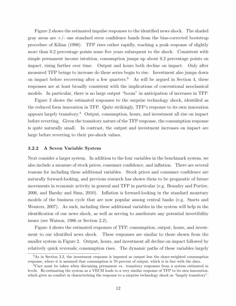
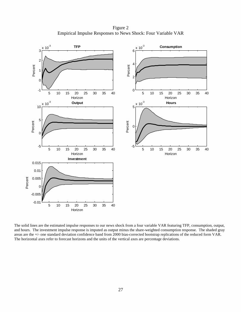
Figure 2 shows the estimated impulse responses to the identified news shock. The shaded

gray areas are +/- one standard error confidence bands from the bias-corrected bootstrap

procedure of Kilian (1998). TFP rises rather rapidly, reaching a peak response of slightly

more than 0.2 percentage points some five years subsequent to the shock. Consistent with

simple permanent income intuition, consumption jumps up about 0.2 percentage points on

impact, rising further over time. Output and hours both decline on impact. Only after

measured TFP beings to increase do these series begin to rise. Investment also jumps down

on impact before recovering after a few quarters.3 As will be argued in Section 4, these

responses are at least broadly consistent with the implications of conventional neoclassical

models. In particular, there is no large output “boom” in anticipation of increases in TFP.

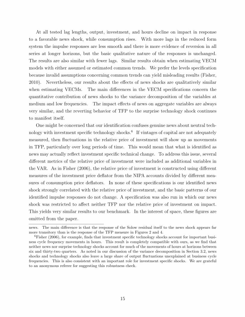
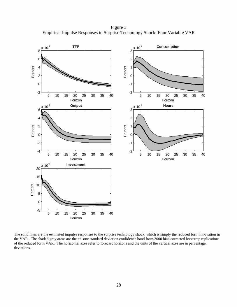
Figure 3 shows the estimated responses to the surprise technology shock, identified as

the reduced form innovation in TFP. Quite strikingly, TFP’s response to its own innovation

appears largely transitory.4 Output, consumption, hours, and investment all rise on impact

before reverting. Given the transitory nature of the TFP response, the consumption response

is quite naturally small. In contrast, the output and investment increases on impact are

large before reverting to their pre-shock values.

3.2.2 A Seven Variable System

Next consider a larger system. In addition to the four variables in the benchmark system, we

also include a measure of stock prices, consumer confidence, and inflation. There are several

reasons for including these additional variables. Stock prices and consumer confidence are

naturally forward-looking, and previous research has shown them to be prognostic of future

movements in economic activity in general and TFP in particular (e.g. Beaudry and Portier,

2006, and Barsky and Sims, 2010). Inflation is forward-looking in the standard monetary

models of the business cycle that are now popular among central banks (e.g. Smets and

Wouters, 2007). As such, including these additional variables in the system will help in the

identification of our news shock, as well as serving to ameliorate any potential invertibility

issues (see Watson, 1986 or Section 2.2).

Figure 4 shows the estimated responses of TFP, consumption, output, hours, and invest-

ment to our identified news shock. These responses are similar to those shown from the

smaller system in Figure 2. Output, hours, and investment all decline on impact followed by

relatively quick reversals; consumption rises. The dynamic paths of these variables largely

3As in Section 2.2, the investment response is imputed as output less the share-weighted consumptionresponse, where it is assumed that consumption is 70 percent of output, which is in line with the data.

4Care must be taken when discussing permanent vs. transitory responses from a system estimated inlevels. Re-estimating the system as a VECM leads to a very similar response of TFP to its own innovation,which gives us comfort in characterizing the response to a surprise technology shock as “largely transitory”.

12

track – as opposed to anticipate – the estimated time path of TFP. With the inclusion of the

additional variables in the system there is somewhat more predictability in the time path of

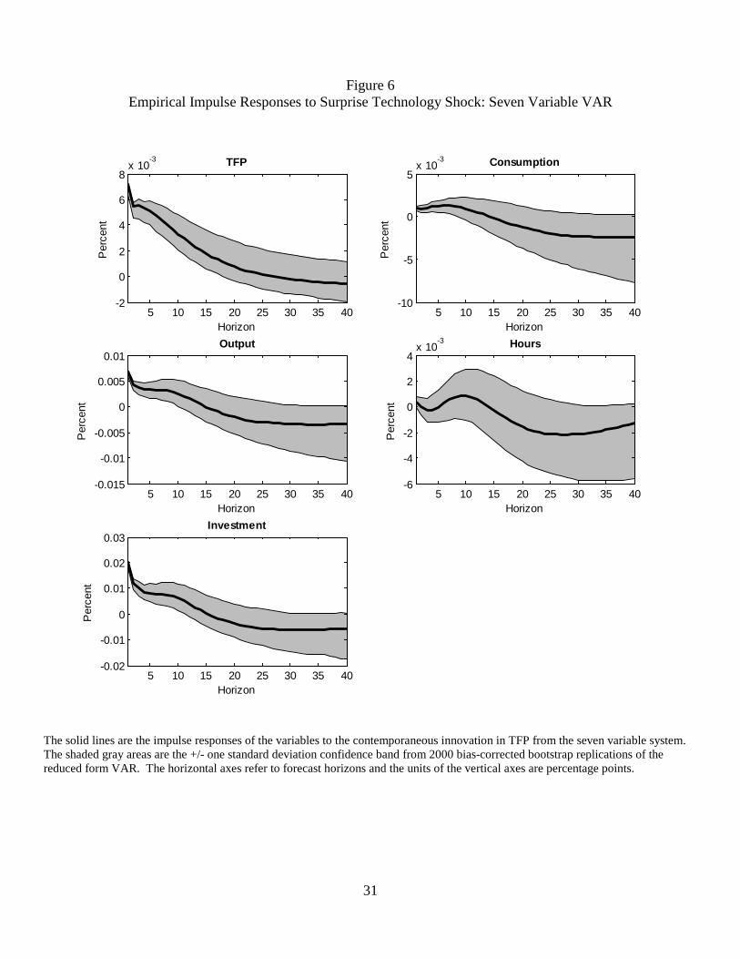
TFP, so that its response is larger here than in Figure 2. Figure 5 shows the responses of

these variables to the surprise technology shock. These are very similar to what is estimated

in the smaller system. In particular, TFP’s response continues to appear largely transitory.

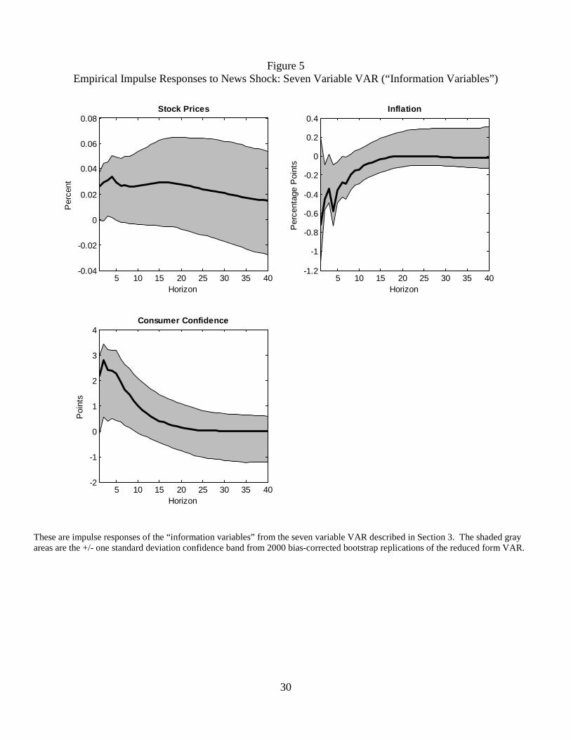
Figure 6 shows the responses of stock prices, inflation, and consumer confidence to a

news shock. Consistent with the results in Beaudry and Portier (2006), stock prices rise

significantly on impact. There is some evidence of reversion at longer horizons, though it

is not possible to reject that the impulse response is consistent with stock prices following

a random walk. Inflation is estimated to fall significantly in response to good news. This

response is broadly consistent with the New Keynesian framework in which current inflation

equals an expected present discounted value of future marginal costs. Consumer confidence

rises on impact, which is consistent with the empirical findings in Barsky and Sims (2010).

Table 1 depicts the share of the forecast error variance of the variables in the seven variable

VAR attributable to our news shock at various horizons. The numbers in parentheses are the

standard errors from the bootstrap replications used to construct the confidence bands for

the impulse responses. Our news shock accounts for more than one quarter of the variance

of TFP at a horizon of four years and more than 40 percent at a horizon of ten years. The

second to last row of the table shows the total contribution to TFP’s forecast error variance

of our news shock and the surprise technology shock. These two shocks combine to explain

roughly 95 percent of the variation in TFP at frequencies up to ten years.

Our news shock accounts for a relatively small share of the forecast error variances of

consumption at short horizons, and a somewhat larger share of the forecast error variance of

output. The shock contributes more significantly to the variance decomposition of hours at

high frequencies and much less so at lower frequencies. At longer horizons our news shock

contributes more significantly to the variance decomposition of the aggregate variables ex-

cluding hours, explaining between ten and forty percent of the variance of output at business

cycle frequencies. Relative to much of the identified VAR literature, these contributions to

the forecast error variance of output are large. This suggests that news shocks are a po-

tentially important component behind economic fluctuations, though not necessarily in the

way that the extant literature has suggested. The final row of the table shows the total

fraction of the forecast variance of output explained by our news and surprise technology

shocks combined. At business cycle frequencies, these two shocks combine to leave more

than 50 percent of the variance of output unexplained. This means that non-technology

shocks (i.e. “demand” shocks) are an important driving force behind fluctuations, a result

which is backed up in both the identified VAR literature and in estimated DSGE models.

13

In order to get a better sense for how important our news shocks have been in explaining

particular episodes, Figure 7 plots an historical decomposition of real output. The subplots

focus in on a one year centered window around the NBER defined recession dates, treating

the 1980 and 1981-1982 recessions as one event. The dashed lines show the simulated value

of output from the seven variable VAR as if our news shocks were the only stochastic distur-

bances. The solid line shows the time path of actual output. In four out of six recessions

(not counting the most recent one, for which there is insufficient data), the simulated time

path of output in response to news shocks is increasing during recessions, not decreasing.

The two exceptions are the 1973-1975 recession and the 1980 recession. In neither of these

events, however, do our news shocks explain a large share of the output decline. On the

basis of these simulations, it is difficult to conclude that news shocks have been a major

driving force behind post-war US recessions.

As will be discussed more in Section 4, most theoretical models have strong testable

predictions concerning the behavior of equilibrium prices in response to news shocks. In

particular, both real wages and real interest rates should rise following a good news shock.

The rise in the wage comes from a reduction in labor supply and the rise in the interest

rate comes from a reduction in savings supply, both resulting from the positive wealth

effect associated with good news. To see whether this prediction is borne out in the data,

measures of both series are included in our empirical VAR. The real wage is measured as

the log of real hourly compensation in the non-farm business sector, and the real interest

rate as the Baa corporate bond yield less expected inflation, where the expected inflation

number from the Michigan Survey of Consumers. These measures are included in our seven

variable VAR, replacing the consumer confidence and inflation measures. Consistent with

model predictions, both rise on impact (figures omitted). The real wage is estimated to

be significantly higher for a number of periods and its long horizon response is of similar

magnitude to the response of output. While statistically insignificant, the interest rate

response is economically large and positive for a number of periods after impact.

3.3 Sensitivity

The result that our news shock induces negative impact comovement among aggregate vari-

ables is robust to alternative lag structures in the reduced form system as well as to various

different assumptions and/or specifications concerning the long run relationships among the

series.5 In the interest of space, these results are only described qualitatively here.

5Our results are also qualitatively robust with alternative measures of observed TFP. Application of ouridentification to a system with the Solow residual in place of the utilization-adjusted TFP measure againfinds negative impact comovement, with output, hours, and investment all declining in anticipation of good

14

At all tested lag lengths, output, investment, and hours decline on impact in response

to a favorable news shock, while consumption rises. With more lags in the reduced form

system the impulse responses are less smooth and there is more evidence of reversion in all

series at longer horizons, but the basic qualitative nature of the responses is unchanged.

The results are also similar with fewer lags. Similar results obtain when estimating VECM

models with either assumed or estimated common trends. We prefer the levels specification

because invalid assumptions concerning common trends can yield misleading results (Fisher,

2010). Nevertheless, our results about the effects of news shocks are qualitatively similar

when estimating VECMs. The main differences in the VECM specifications concern the

quantitative contribution of news shocks to the variance decomposition of the variables at

medium and low frequencies. The impact effects of news on aggregate variables are always

very similar, and the reverting behavior of TFP to the surprise technology shock continues

to manifest itself.

One might be concerned that our identification confuses genuine news about neutral tech-

nology with investment specific technology shocks.6 If vintages of capital are not adequately

measured, then fluctuations in the relative price of investment will show up as movements

in TFP, particularly over long periods of time. This would mean that what is identified as

news may actually reflect investment specific technical change. To address this issue, several

different metrics of the relative price of investment were included as additional variables in

the VAR. As in Fisher (2006), the relative price of investment is constructed using different

measures of the investment price deflator from the NIPA accounts divided by different mea-

sures of consumption price deflators. In none of these specifications is our identified news

shock strongly correlated with the relative price of investment, and the basic patterns of our

identified impulse responses do not change. A specification was also run in which our news

shock was restricted to affect neither TFP nor the relative price of investment on impact.

This yields very similar results to our benchmark. In the interest of space, these figures are

omitted from the paper.

news. The main difference is that the response of the Solow residual itself to the news shock appears farmore transitory than is the response of the TFP measure in Figures 2 and 4.

6Fisher (2006), for example, finds that investment specific technology shocks account for important busi-ness cycle frequency movements in hours. This result is completely compatible with ours, as we find thatneither news nor surprise technology shocks account for much of the movements of hours at horizons betweensix and thirty-two quarters. As noted in our discussion of the variance decomposition in Section 3.2, newsshocks and technology shocks also leave a large share of output fluctuations unexplained at business cyclefrequencies. This is also consistent with an important role for investment specific shocks. We are gratefulto an anonymous referee for suggesting this robustness check.

15

3.4 Relation with Earlier Work

The most well-known empirical work in the news shock literature are papers are by Beaudry

and Portier (2006), Beaudry, Dupaigne, and Portier (2008), and Beaudry and Lucke (2010).

These authors estimate two to five variable systems featuring measures of TFP, stock prices,

and other macroeconomic aggregates. They propose two alternative orthogonalization

schemes aimed at isolating news shocks – the first is to associate the news shock with

the stock price innovation orthogonalized with respect to TFP, and the second combines

short and long run restrictions to identify the news shock. These authors argue that both

orthogonalization schemes yield very similar results. They find that news shocks lead to

positive conditional comovement among macroeconomic aggregates on impact, that aggre-

gate variables strongly anticipate movements in technology, and that news shocks account

for the bulk of the variance of aggregate variables at business cycle frequencies.

The conditions under which either of these orthogonalization schemes are valid are en-

compassed by our identification strategy. In particular, were the conditions required for the

pure recursive identification satisfied, our identification would (asymptotically) identify the

same shock and impulse responses. Likewise, their long run identifying assumption in the

second orthogonalization scheme rests on the same implicit assumption underlying our iden-

tification – that a limited number of shocks account for variation in measured technology.

It is, however, more restrictive in the sense that it imposes that both kind of technology

shocks permanently impact the level of TFP. Ours, in contrast, only imposes that the two

technology shocks together explain the bulk of movements in TFP, without taking a stand

on whether both permanently impact TFP.

In practice, there is a large quantitative and qualitative difference between our results

and theirs in the estimated effects of news shocks on TFP itself. The shock identified

by these authors typically does not have any noticeable effect on TFP for several years.

Indeed, Beaudry and Portier (2006) note that “growth beyond its [TFP’s] initial level takes

somewhere between 12 and 16 quarters” (p. 1303) following a news shock, while in Beaudry,

Dupaigne, and Portier (2008), they state “it [news shock] has almost no impact on TFP

during the first five years” (p. 3). In contrast, our news shock begins to affect TFP soon

after impact, and explains TFP movements well at both short and long horizons.

That these authors’ identified shock has such a delayed effect on TFP makes its inter-

pretation as a news shock problematic. Application of their identification strategies reveals

that roughly one-third of the TFP forecast error variance is left unexplained at business cycle

frequencies. In other words, some other structural shock orthogonal to TFP’s innovation

potentially accounts for twice as much variation in TFP at these frequencies than does what

these authors deem the news shock. In comparison, our identification leaves less than 5 per-

16

cent of TFP’s variance unaccounted for at business cycle frequencies, as shown in the second

to last row of Table 1. Our identification strategy and results are more consistent with

the nascent theoretical literature on news shocks, which generally assumes delays between

arrival of news and adoption of less than two years.

An alternative approach to the VAR-based methodology of studying the implications of

news shocks for aggregate variables would be the estimation of a fully specified DSGE model.

This is the approach taken by Schmitt-Grohe and Uribe (2008), who argue that news shocks

about future technology are quantitatively important for understanding fluctuations. While

there are some differences (particularly in the impact behavior of output and investment

to news), our conclusions about the importance of news shocks at medium frequencies are

similar. In practice, estimation of a fully specified model in this context is problematic, as

there is no consensus on what the appropriate theoretical structure is in which news shocks

have a chance to be the primary driver of output fluctuations.

4 Discussion

This section discusses our results, places them in the context of the existing literature, points

out some unresolved issues, and suggests avenues for future research.

A large literature has developed that seeks to develop theoretical models which gener-

ate positive impact comovement in response to good news. This has not proven to be a

particularly easy task. Among papers in this growing literature are Beaudry and Portier

(2004), Den Haan and Kaltenbrunner (2006), and Jaimovich and Rebelo (2009). Our em-

pirical results suggest that this excessive focus on the impact effects of news shocks has been

somewhat misplaced. A similar point is made by Leeper and Walker (2011).

To make this point concrete, we show here that a simple, textbook neoclassical growth

model augmented with news shocks is capable of generating impulse responses which are

very similar to those that are estimated in the data. The model is a special case of the one

presented in Section 2.2 in which there are no investment adjustment costs. So as to better

fit the data, the process for technology is modified so that news diffuses slowly into TFP:

lnAt = gt−1 + lnAt−1 (20)

gt = ρgt−1 + ut (21)

(22) is simply a “smooth” version of the news process shown in (2) above. Given the

17

timing assumption, ut can be interpreted as a news shock since it has no contemporaneous

effect on the level of technology.

The parameters of the model are chosen to fit the estimated impulse responses of TFP,

consumption, output and hours to the news shock from the seven variable VAR. The impulse

responses from this parameterized model are shown as the dashed line in Figure 8, along

with the empirical impulse responses (solid line) and confidence regions (shaded gray) from

Figure 4. The model’s impulse responses lie very closely to those estimated in the data at

all horizons and are completely contained by the shaded confidence regions. In short, this

simple model appears to provide a very good fit to the data, at least along this dimension.

The various “fixes” that have been proposed to deal with negative impact comovement of

quantities in response to news shocks appear unnecessary.

The dimension along which the model does not fare well is in the behavior of the value

of the firm. In the data, stock prices rise in response to our identified news shock, whereas

in the model they fall. In the version of the model without any adjustment costs, the value

of the firm is just equal to the capital stock, which falls for a few periods in response to

good news. Even with substantial adjustment costs the value of the firm will still initially

fall due to the rise in the real interest rate. Christiano, Ilut, Motto, and Rostagno (2008)

document this phenomenon in detail. Walentin (2009) proposes that limited enforcement

of financial contracts can potentially help generate stock price appreciations in anticipation

of higher future productivity. Jinnai (2010) successfully builds a model in which the value

of the firm rises in response to news even though investment falls. Our empirical results

along these dimensions should help inform researchers building detailed DSGE models.

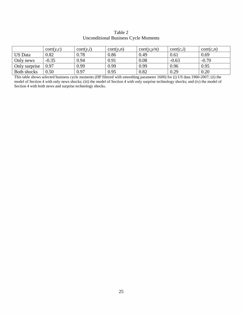
Given that positive comovement among aggregate variables is a ubiquitous feature of the

data, news shocks as estimated here cannot be the sole driving force behind fluctuations.

The first interior row of Table 2 shows selected correlations among HP filtered aggregate

variables for the period 1960-2007 (using smoothing parameter 1600). These correlations

are all positive and strong, but many are far from one. The second interior row of the

table shows the correlations that would obtain if the news shock were the only stochastic

disturbance in the simple model as presented above (parameterized as described). While the

correlations between output and investment and output and hours are reasonably close to

those in the data, the correlations involving consumption and other aggregates are negative.

This is clearly at odds with the data.

The next row of the table shows the resulting moments if a surprise technology shock were

the only stochastic disturbance in the model. The shock is assumed to follow a stationary

AR(1) process with autoregressive coefficient 0.98 and standard deviation of 0.75 percent.

This calibration produces an impulse response of technology that matches the observed

18

response of TFP to its own innovation in our VARs. Here the resulting correlations are all

nearly one, which is too high relative to the data. The final row shows the correlations that

result if both the permanent news shock and the transitory surprise technology shock are

included in the model. Relative to the one shock model, the two shock version fits better

on many dimensions – the correlations are all positive but not too close to one.

The above exercise is meant to be illustrative but makes two related points. First,

conventional business cycle models are capable of qualitatively matching the dynamic, con-

ditional responses of many aggregate variables to news about future technology. Second,

even if news shocks do not induce positive comovement on impact, they can nevertheless

be an important part of the data generating process and can help explain some features of

the data. In particular, the presence of news shocks can work to lower the correlations

among aggregate variables that obtain in a simple one shock RBC model, in much the same

way that, for example, government spending or distortionary tax shocks do (Christiano and

Eichenbaum, 1992, and McGrattan, 1994). New research points out several additional chan-

nels by which news shocks help to better fit the data. Kurmann and Otrok (2010), using

a similar methodology to that pursued here, argue that news shocks help explain the slope

of the term structure of interest rates. Mertens (2010) shows how news shocks can help

account for the comovement between output and interest rates that has puzzled economists

since King and Watson (1996).

Our results suggest that research should move more towards medium frequencies and in

finding structural explanations for news, and away from trying to resolve impact comovement

problems. News shocks (or more generally slow technological diffusion) can be an important

propagation mechanism, even if the shocks do not induce high frequency comovement (An-

dolfatto and MacDonald, 1998, and Leeper and Walker, 2011). Most of the theoretical work

in the news area assumes that good news is “manna from heaven” – that is, agents receive

word in advance that aggregate technology will exogenously change at some point in the

future. This assumption seems unrealistic; searching for a deeper structural explanation for

what has been empirically identified and labeled as “news” is a promising avenue for future

work. Schmitt-Grohe and Uribe (2011), for example, argue that a common trend shock to

both neutral and investment specific technology is an important driving force behind fluctu-

ations. The impulse responses of aggregate variables to their common trend shock are very

similar to the responses to our news shock.

19

5 Conclusion

The news driven business cycle hypothesis offers the tantalizing possibility that business

cycles could emerge absent any (ex-post) change in fundamentals. If good news about the

future can set off a boom today, then a realization worse than anticipated can set off a

bust. For this story to work, however, good news about the future must induce broad-based

comovement, which is not the prediction of standard macro models. Existing empirical

evidence suggesting that news shocks do lead to broad-based comovement has spawned a

new literature searching for theoretical frameworks capable of delivering business cycle-like

behavior when driven by news shocks about future technology.

This paper has taken a closer look at the empirical evidence in favor of this theory of

fluctuations. It implemented a novel empirical approach for identifying news shocks that is

directly based on the implications of theoretical models of news driven business cycles. In

contrast to the existing literature, a good realization of our news shock is associated with

an increase in consumption and impact declines in output, hours, and investment. After

impact, aggregate variables largely track, as opposed to anticipate, predicted movements

in measured TFP. The estimated impulse responses are broadly consistent with the im-

plications of standard macro models. While important at medium to low frequencies, an

historical decomposition reveals that news shocks have not been a major source of post-war

US recessions. News shocks nevertheless do help to explain several features of the data.

While we find no evidence to support the “boom-bust” story advanced by the literature,

incorporating news shocks into existing models and seeking deeper structural explanations

for what manifests itself as “news” seem like promising avenues for future research.

20

References

[1] Andolfatto, D., MacDonald, G., 1998. Technology diffusion and aggregate dynamics.

Review of Economic Dynamics 1 (2), 338-370.

[2] Barro, R., King, R., 1984. Time separable preferences and intertemporal substitution

models of business cycles. Quarterly Journal of Economics 99 (4), 817-839.

[3] Barsky, R., Sims, E., 2010. Information, animal spirits, and the meaning of innovations

in consumer confidence. NBER Working Paper 15049.

[4] Basu, S., Fernald, J., Kimball, M., 2006. Are technology improvements contractionary?

American Economic Review 96 (5), 1418-1448.

[5] Beaudry, P., Lucke, B., 2010. Letting different views about business cycles compete.

NBER Macroeconomics Annual 2009 24, 413-455.

[6] Beaudry, P., Portier, F., 2004. An exploration into Pigou’s theory of cycles. Journal

of Monetary Economics 51 (6), 1183-1216.

[7] Beaudry, P., Portier, F., 2006. News, stock prices, and economic fluctuations. American

Economic Review 96 (4), 1293-1307.

[8] Beaudry, P., Dupaigne, M., Portier, F., 2008. The international propagation of news

shocks. Unpublished manuscript, University of British Columbia.

[9] Blanchard, O., L’Hullier, J., Lorenzoni, G., 2009. News, noise, and fluctuations: an

empirical exploration. NBER Working Paper 15015.

[10] Chari, V., Kehoe, P., McGrattan, E., 2008. Are structural VARs with long run restric-

tions useful in developing business cycle theory? Journal of Monetary Economics 55 (8),

1337-1352.

[11] Christiano, L., Eichenbaum, M., 1992. Current real business cycle theories and aggregate

labor market fluctuations. American Economic Review 82 (3), 430-450.

[12] Christiano, L., Ilut, C., Motto, R., Rostagno, M., 2008. Monetary policy and stock

market boom bust cycles. Unpublished manuscript, Northwestern University.

[13] Cochrane, J., 1994. Shocks. Carnegie-Rochester Conference Series on Public Policy 41

(1), 295-364.

21

[14] Den Haan, W., Kaltenbrunner, G., 2006. Anticipated growth and business cycles in

matching models. Unpublished manuscript, Euro Area Business Cycle Network.

[15] Faust, J., 1998. The robustness of identified VAR conclusions about money. Carnegie-

Rochester Conference Series on Public Policy 49 (1), 207-244.

[16] Faust, J., Leeper, E., 1997. When do long run identifying restrictions give reliable

results? Journal of Business and Economic Statistics 15 (3), 345-353.

[17] Fernandez-Villaverde, J., Rubio-Ramirez, J. Sargent, T., Watson, M., 2007. ABCs (and

Ds) of understanding VARs. American Economic Review 97 (3), 1021-1026.

[18] Fisher, J., 2006. The dynamic effects of neutral and investment specific technology

shocks. Journal of Political Economy 114 (3), 413-451.

[19] Fisher, J., 2010. Comment on: Letting different views about business cycles compete.

NBER Macroeconomics Annual 2009 24, 457-474.

[20] Francis, N., Owyang, M., Roush, J., 2007. A flexible finite horizon identification of

technology shocks. Unpublished manuscript, Federal Reserve Bank of St. Louis.

[21] Hamilton, J., 1994. Time series analysis. Princeton University Press, Princeton.

[22] Jaimovich, N., Rebelo, S., 2009. Can news about the future drive the business cycle?

American Economic Review 99 (4), 1097-1118

[23] Jinnai, R., 2010. News shocks, product innovations, and business cycles. Unpublished

manuscript, Texas A & M University.

[24] Kilian, L., 1998. Small sample confidence intervals for impulse response functions.

Review of Economics and Statistics 80 (2), 218-230.

[25] King, R., Watson, M., 1996. Money, prices, interest rates and the business cycle.

Review of Economics and Statistics 78 (1), 35-53.

[26] Kurmann, A., Otrok, C., 2010. News shocks and the slope of the term structure of

interest rates. Unpublished manuscript, University of Virginia.

[27] Leeper, E., Walker, T., 2011. Information flows and news driven business cycles. Review

of Economic Dynamics 14 (1), 55-71.

[28] Leeper, E., Walker, T., Yang, S.C., 2008. Fiscal foresight: analytics and econometrics.

NBER Working Paper 14028.

22

[29] McGrattan, E., 1994. The macroeconomic effects of distortionary taxation. Journal of

Monetary Economics 33 (3), 573-601.

[30] Mertens, E., 2010. Structural shocks and the comovements between output and interest

rates. Journal of Economic Dynamics and Control 34 (6), 1171-1186.

[31] Pigou, A., 1927. Industrial fluctuations. MacMillan, London.

[32] Schmitt-Grohe, S., Uribe, M., 2008. What’s news in the business cycle? NBER Working

Paper 14215.

[33] Schmitt-Grohe, S., Uribe, M., 2011. Business cycles with a common trend in neutral

and investment specific productivity. Review of Economic Dynamics 14 (1), 122-135.

[34] Sims, C., Zha, T., 2006. Does monetary policy generate recessions? Macroeconomic

Dynamics 10 (2), 231-272.

[35] Smets, F., Wouters, R., 2007. Shocks and frictions in US business cycles: a Bayesian

DSGE approach. American Economic Review 97 (3), 586-606.

[36] Uhlig, H., 2003. What drives GNP? Unpublished manuscript, Euro Area Business Cycle

Network.

[37] Uhlig, H., 2004. Do technology shocks lead to a fall in total hours worked? Journal of

the European Economic Association 2 (2-3), 361-371.

[38] Walentin, K., 2009. Expectation driven business cycles with limited enforcement.

Sveriges Riksbank Working Paper No. 229.

[39] Watson, M., 1986. Vector autoregressions and cointegration. In: Engle, R. and McFad-

den, D. (Eds.), Handbook of Econometrics. Elsevier, Amsterdam, pp. 2843-2915.

23

24

Table 1

Share of Forecast Error Variance Attributable to News Shock: Seven Variable VAR

h=0 h=4 h=8 h=16 h=24 h=40 TFP 0.000 0.062 0.126 0.269 0.366 0.454 (0.00) (0.06) (0.11) (0.14) (0.15) (0.16) Consumption 0.050 0.234 0.377 0.493 0.524 0.507 (0.09) (0.18) (0.24) (0.27) (0.27) (0.26) Output 0.111 0.091 0.242 0.382 0.429 0.431 (0.07) (0.10) (0.18) (0.23) (0.24) (0.24) Hours 0.622 0.200 0.105 0.092 0.094 0.089 (0.23) (0.16) (0.13) (0.15) (0.16) (0.15) Stock Price 0.140 0.200 0.185 0.189 0.193 0.181 (0.17) (0.20) (0.20) (0.21) (0.22) (0.21) Confidence 0.245 0.343 0.353 0.333 0.310 0.286 (0.21) (0.22) (0.22) (0.22) (0.20) (0.18) Inflation 0.138 0.220 0.226 0.205 0.191 0.180 (0.18) (0.18) (0.15) (0.15) (0.14) (0.14) Total TFP 1.000 0.948 0.943 0.951 0.948 0.910 Total Output 0.731 0.282 0.364 0.451 0.491 0.520 The letter h refers to the forecast horizon. The numbers denote the fraction of the total forecast error variance of each variable assigned to our identified news shock. The numbers in parentheses are the standard deviation of a bias-corrected bootstrap simulation. The row titled “Total TFP” shows the total forecast error variance of measured TFP explained by the news shock and the TFP innovation combined. The row titled “Total Output” show the total forecast error variance of output explained by the news shock and the TFP innovation combined.

25

Table 2

Unconditional Business Cycle Moments

corr(y,c) corr(y,i) corr(y,n) corr(y,y/n) corr(c,i) corr(c,n) US Data 0.82 0.78 0.86 0.49 0.61 0.69 Only news -0.35 0.94 0.91 0.08 -0.63 -0.70 Only surprise 0.97 0.99 0.99 0.99 0.96 0.95 Both shocks 0.50 0.97 0.95 0.82 0.29 0.20 This table shows selected business cycle moments (HP filtered with smoothing parameter 1600) for (i) US data 1960-2007; (ii) the model of Section 4 with only news shocks; (iii) the model of Section 4 with only surprise technology shocks; and (iv) the model of Section 4 with both news and surprise technology shocks.

26

Figure 1 Model and Monte Carlo Estimated Impulse Responses to News Shocks

Horizon

Per

cent

Technology

0 5 10 15 20

0

0.2

0.4

Consumption

Horizon

Per

cent

0 5 10 15 200

0.2

0.4

Output

Horizon

Per

cent

0 5 10 15 20-0.2

0

0.2

0.4

0.6

0.8Hours

Horizon

Per

cent

0 5 10 15 20-0.2

-0.1

0

0.1

0.2

Investment

Horizon

Per

cent

0 5 10 15 20-0.5

0

0.5

1

1.5

The solid line shows the theoretical impulse response to a news shock from the model presented in Section 2.2. The dashed line is the average estimated impulse responses from a Monte Carlo simulation with 2000 repetitions and 191 observations per repetition. The estimated VAR includes TFP, consumption, output, and hours, all in levels. The investment response is imputed as the output response less the share-weighted consumption response. The shaded gray areas are the one +/- one standard deviation confidence bands from the 2000 Monte Carlo repetitions. The horizontal axes refer to forecast horizons and the units of the vertical axes are percentage deviations (times 100).

27

Figure 2 Empirical Impulse Responses to News Shock: Four Variable VAR

Horizon

Per

cent

TFP

5 10 15 20 25 30 35 40-1

0

1

2

3x 10

-3 Consumption

Horizon

Per

cent

5 10 15 20 25 30 35 400

2

4

6x 10

-3

Output

Horizon

Per

cent

5 10 15 20 25 30 35 40-5

0

5

10x 10

-3 Hours

Horizon

Per

cent

5 10 15 20 25 30 35 40-5

0

5x 10

-3

Investment

Horizon

Per

cent

5 10 15 20 25 30 35 40-0.01

-0.005

0

0.005

0.01

0.015

The solid lines are the estimated impulse responses to our news shock from a four variable VAR featuring TFP, consumption, output, and hours. The investment impulse response is imputed as output minus the share-weighted consumption response. The shaded gray areas are the +/- one standard deviation confidence band from 2000 bias-corrected bootstrap replications of the reduced form VAR. The horizontal axes refer to forecast horizons and the units of the vertical axes are percentage deviations.

28

Figure 3 Empirical Impulse Responses to Surprise Technology Shock: Four Variable VAR

TFP

Horizon

Per

cent

5 10 15 20 25 30 35 40-2

0

2

4

6

8x 10

-3 Consumption

Horizon

Per

cent

5 10 15 20 25 30 35 40-2

-1

0

1

2

3x 10

-3

Output

Horizon

Per

cent

5 10 15 20 25 30 35 40-4

-2

0

2

4

6x 10

-3 Hours

Horizon

Per

cent

5 10 15 20 25 30 35 40-2

-1

0

1

2

3x 10

-3

Investment

Horizon

Per

cent

5 10 15 20 25 30 35 40-5

0

5

10

15

20x 10

-3

The solid lines are the estimated impulse responses to the surprise technology shock, which is simply the reduced form innovation in the VAR. The shaded gray areas are the +/- one standard deviation confidence band from 2000 bias-corrected bootstrap replications of the reduced form VAR. The horizontal axes refer to forecast horizons and the units of the vertical axes are in percentage deviations.

29

Figure 4 Empirical Impulse Responses to News Shock: Seven Variable VAR

TFP

Horizon

Per

cent

5 10 15 20 25 30 35 400

2

4

6x 10

-3 Consumption

Horizon

Per

cent

5 10 15 20 25 30 35 40-5

0

5

10x 10

-3

Output

Horizon

Per

cent

5 10 15 20 25 30 35 40-5

0

5

10

15x 10

-3 Hours

Horizon

Per

cent

5 10 15 20 25 30 35 40-0.01

-0.005

0

0.005

0.01

Investment

Horizon

Per

cent

5 10 15 20 25 30 35 40-0.02

-0.01

0

0.01

0.02

0.03

The solid line is the estimated impulse response to a news shock from a seven variable VAR featuring TFP, consumption, output, hours, stock prices, consumer confidence, and inflation. The shaded gray areas are the +/- one standard deviation confidence band from 2000 bias-corrected bootstrap replications of the reduced form VAR. The horizontal axes refer to forecast horizons and the units of the vertical axes are percentage deviations.

30

Figure 5 Empirical Impulse Responses to News Shock: Seven Variable VAR (“Information Variables”)

Stock Prices

Horizon

Per

cent

5 10 15 20 25 30 35 40-0.04

-0.02

0

0.02

0.04

0.06

0.08Inflation

HorizonP

erce

ntag

e P

oint

s

5 10 15 20 25 30 35 40-1.2

-1

-0.8

-0.6

-0.4

-0.2

0

0.2

0.4

Consumer Confidence

Horizon

Poi

nts

5 10 15 20 25 30 35 40-2

-1

0

1

2

3

4

These are impulse responses of the “information variables” from the seven variable VAR described in Section 3. The shaded gray areas are the +/- one standard deviation confidence band from 2000 bias-corrected bootstrap replications of the reduced form VAR.

31

Figure 6 Empirical Impulse Responses to Surprise Technology Shock: Seven Variable VAR

TFP

Horizon

Per

cent

5 10 15 20 25 30 35 40-2

0

2

4

6

8x 10

-3 Consumption

Horizon

Per

cent

5 10 15 20 25 30 35 40-10

-5

0

5x 10

-3

Output

Horizon

Per

cent

5 10 15 20 25 30 35 40-0.015

-0.01

-0.005

0

0.005

0.01Hours

Horizon

Per

cent

5 10 15 20 25 30 35 40-6

-4

-2

0

2

4x 10

-3

Investment

Horizon

Per

cent

5 10 15 20 25 30 35 40-0.02

-0.01

0

0.01

0.02

0.03

The solid lines are the impulse responses of the variables to the contemporaneous innovation in TFP from the seven variable system. The shaded gray areas are the +/- one standard deviation confidence band from 2000 bias-corrected bootstrap replications of the reduced form VAR. The horizontal axes refer to forecast horizons and the units of the vertical axes are percentage points.

32

Figure 7 Historical Simulation of Output

-10.94

-10.93

-10.92

-10.91

-10.90

-10.89

-10.88

-10.87

-10.86

1969Q1 1969Q3 1970Q1 1970Q3 1971Q1 1971Q3-10.90

-10.88

-10.86

-10.84

-10.82

-10.80

-10.78

1973Q1 1973Q3 1974Q1 1974Q3 1975Q1 1975Q3 1976Q1

Actual GDP Simulated GDP

-10.80

-10.78

-10.76

-10.74

-10.72

-10.70

-10.68

-10.66

-10.64

1979 1980 1981 1982 1983-10.56

-10.54

-10.52

-10.50

-10.48

-10.46

1989Q3 1990Q1 1990Q3 1991Q1 1991Q3 1992Q1

-10.38

-10.36

-10.34

-10.32

-10.30

-10.28

-10.26

2000Q1 2000Q3 2001Q1 2001Q3 2002Q1 2002Q3

1969-1970 Recession 1973-1975 Recession

1980 and 1981-1982 Recessions1990-1991 Recession

2001 Recession

In these figures the solid line is the actual level of log real output. The dashed line is the simulated log level if news shocks were the only stochastic disturbance. The shaded areas correspond to recession dates as defined by the NBER. The units of the vertical axes are the log of output per capita. The horizontal axes refer to dates.

33

Figure 8

Empirical Impulse Responses vs. RBC Model Impulse Responses

Technology

Horizon

Per

cent

5 10 15 200

2

4

6x 10

-3 Consumption

Horizon

Per

cent

5 10 15 20-5

0

5

10x 10

-3

Output

Horizon

Per

cent

5 10 15 20-5

0

5

10

15x 10

-3 Hours

Horizon

Per

cent

5 10 15 20-0.01

-0.005

0

0.005

0.01

Investment

Horizon

Per

cent

5 10 15 20-0.02

-0.01

0

0.01

0.02

0.03Value of the Firm

Horizon

Per

cent

5 10 15 20-0.02

0

0.02

0.04

0.06

0.08

The solid lines are the estimation empirical responses, identical to those shown in Figure 4. The shaded gray areas are the +/- one standard error bootstrap confidence bands. The dashed lines are the theoretical responses from the best-fitting parameterization of the simple RBC model. The horizontal axes refer to forecast horizons and the units of the vertical axes are percentage deviations.