newton power flow methods for unbalanced three-phase...
TRANSCRIPT

Article
Newton Power Flow Methods for UnbalancedThree-Phase Distribution Networks
Baljinnyam Sereeter *, Kees Vuik and Cees Witteveen
Faculty of Electrical Engineering, Mathematics and Computer Science, Delft University of Technology,Mekelweg 4, 2628 CD Delft, The Netherlands; [email protected] (K.V.); [email protected] (C.W.)* Correspondence: [email protected]; Tel.: +31-015-2781-692
Received: 25 August 2017; Accepted: 12 October 2017; Published: 20 October 2017
Abstract: Two mismatch functions (power or current) and three coordinates (polar, Cartesian andcomplex form) result in six versions of the Newton–Raphson method for the solution of powerflow problems. In this paper, five new versions of the Newton power flow method developed forsingle-phase problems in our previous paper are extended to three-phase power flow problems.Mathematical models of the load, load connection, transformer, and distributed generation (DG)are presented. A three-phase power flow formulation is described for both power and currentmismatch functions. Extended versions of the Newton power flow method are compared with thebackward-forward sweep-based algorithm. Furthermore, the convergence behavior for differentloading conditions, R/X ratios, and load models, is investigated by numerical experiments onbalanced and unbalanced distribution networks. On the basis of these experiments, we conclude thattwo versions using the current mismatch function in polar and Cartesian coordinates perform thebest for both balanced and unbalanced distribution networks.
Keywords: power flow analysis; Newton–Raphson method; three-phase; unbalanced; distributionnetworks
1. Introduction
The electrical power system is one of the most complex system types built by engineers [1].Traditionally, electricity was generated by a small number of large bulk power plants that use coal, oil,or nuclear fission and was delivered to consumers through the power system in a one-way direction.Due to the modernization of the existing grid, a large number of new grid elements and functionsincluding smart meters, smart appliances, renewable energy resources, and storage devices are beingintegrated into the grid. Thus, the existing electrical grid is changing rapidly and becoming more andmore complex to control. A smart grid (SG) is offered as the solution to this problem [2–4].
In a smart grid, most of the new grid elements are directly connected to the distribution networkwhich requires new types of operation and maintenance. The distribution network has been consideredas a passive network that totally depends on the transmission network for control and regulation ofsystem parameters. Conventionally, the power flow in the distribution system was one-way traffic(vertical) from the substation (only source) to the end of the feeders. However, the utilization ofdistributed generation (DG) made the distribution network active in the sense that the distributionnetwork can generate electrical power in the network and transfer the extra power to the transmissionnetwork. This changes the direction of the power flow in networks into two-way traffic (horizontal).Therefore, central grid operators or transmission system operators (TSOs) of the power system musthave different approaches for maintaining and operating the electrical grid because in this case,the main purpose of the operator has been adjusted to interconnect the various active distributionnetworks. As the distribution network becomes more active, there is an increasing role of distribution
Energies 2017, 10, 1658; doi:10.3390/en10101658 www.mdpi.com/journal/energies

Energies 2017, 10, 1658 2 of 20
system operators (DSOs). For efficient operation and planning of the power system, it is essential toknow the system steady state conditions for various load demands.
A power flow computation that determines the steady state behavior of the network is one ofthe most important tools for grid operators. The solution of power flow computation can be used toassess whether the power system can function properly for the given generation and consumption.Traditionally, power flow computations were calculated only in the transmission network andthe distribution networks were aggregated as buses in the power system model. However, in the newoperation and maintenance of the distribution network, the power flow problem computation must bedone on the distribution network as well.
A reliable distribution power flow solution method will be required to solve a three-phase powerflow problem in unbalanced distribution networks integrated with distributed generations and activeresources (i.e., renewable power generations, storage devices, and electric vehicles etc.) [5,6]. Thereare conventional power flow solution techniques for transmission networks, such as Gauss–Seidel(GS), Newton power flow (NR), and fast decoupled load flow (FDLF) [7–9] which are widely used forpower system operation, control and planning. However, these conventional power flow methodsdo not always converge when they are applied to the distribution power flow problem due to somespecial features of the distribution network:
• Radial or weakly meshed (radial network with a few simple loops) structure:In general, a transmission network is operated in a meshed structure, whereas a distributionnetwork is operated in a radial structure where there are no loops in the network and each bus isconnected to the source via exactly one path.
• High R/X ratio:Transmission lines of the distribution network have a wide range of resistance R and reactanceX values. Therefore, R/X ratios in the distribution network are relatively high compared to thetransmission network.
• Multi-phase power flow and unbalanced loads:A single-phase representation is used for power flow analysis on transmission network whichis assumed to be a balanced network. Unlike the transmission network, a distribution networkmust use a three-phase power flow analysis due to the unbalanced loads.
• Distributed generations:Unlike conventional power plants connected to the transmission network, DGs have fluctuatingpower output that is difficult to predict and control since it is strongly dependent onweather conditions.
Systems with the above features create ill-conditioned systems of nonlinear algebraic equationsthat cause numerical problems for the conventional methods [10–12]. Many methods have beendeveloped on distribution power flow analysis and generally they can be divided into two maincategories as:
• Modification of conventional power flow solution methods [13–33]:Methods in this category are generally a proper modification of existing methods such as GS, NRand FDLF.
• Backward–forward sweep (BFS)-based algorithms [34–61]:BFS-based algorithms generally take an advantage of the radial network topology. The method isan iterative process in which at each iteration two computational steps are performed, a forwardand a backward sweep. The forward sweep is mainly the node voltage calculation and thebackward sweep is the branch current or power, or the admittance summation.
Several reviews on distribution power flow solution methods can be found in [5,6,62–64].In this paper, we focus on the Newton based power flow methods for balanced and unbalanced
distribution networks with a general topology. Depending on the problem formulation (poweror current mismatch) and specification of the coordinates (polar, Cartesian and complex form),

Energies 2017, 10, 1658 3 of 20
the Newton–Raphson method can be applied in six different ways as a solution method for powerflow problems. We refer to [65] for more details on all six versions of the Newton power flow method.In [65], the existing versions of the Newton power flow method [8,18,66] are compared with thenewly developed/improved versions of the Newton power flow method (Cartesian power mismatch,complex power mismatch, polar current mismatch, Cartesian current mismatch, and complex currentmismatch) for single-phase power flow problems in balanced transmission and distribution networks.It is concluded in [65] that the newly developed/improved versions have better performance than theexisting versions of the Newton power flow method.
Therefore, we want to extend the Newton power flow methods developed for a single-phaseproblem in [65] to three-phase power flow problems. In this paper, only the polar current mismatchversion is explained in detail for a three-phase power flow problem and the remaining versionscan be derived similarly. Moreover, all six versions are implemented and compared with the BFSalgorithm [43] for both balanced and unbalanced distribution networks. Different load models,loading conditions, and R/X ratios are considered in order to analyze the convergence ability of allextended versions. The key contribution of this work is new formulations of the Newton power flowmethod. Compared to existing versions of the Newton power flow method, our versions use differentequations for PV buses in the Jacobian matrix that result in better convergence and robust performance.We present how these versions can be applied to unbalanced distribution networks by studying loads,three-phase load connections, three-phase transformers, and DGs.
This paper is structured as follows. In Section 2, mathematical models of the power system, load,three-phase load connection, three-phase transformer, and DG are introduced. Section 3 mathematicallydescribes the three-phase power flow problem. The Newton power flow method, the polar andthe current mismatch formulations, and the polar current mismatch version are explained for thethree-phase power flow problem in Section 4. The comparison result of all the versions of the Newtonpower flow method with BFS algorithm in balanced and unbalanced distribution networks is presentedin Section 5. Finally, the conclusions are given in Section 6.
2. Power System Model
Power systems are modeled as a network of buses (nodes) and branches (transmission lines),whereas a network bus represents a system component such as a generator, load, and transmissionsubstation, etc. There are three types of network buses such as a slack bus, a generator bus (PV bus)and a load bus (PQ bus). Each bus in the power network is fully described by the following fourelectrical quantities:
• |Vi| : the voltage magnitude• δi : the voltage phase angle• Pi : the active power• Qi : the reactive power
Depending on the type of the bus, two of the four electrical quantities are specified as shownin Table 1.
Table 1. Network bus type. i: index of the bus; Ng: number of generator buses; N: total number ofbuses in the network.
Bus Type Number of Buses Known Unknown
slack node or swing bus 1 |Vi|, δi Pi, Qigenerator node or PV bus Ng Pi, |Vi| Qi, δi
load node or PQ bus N − Ng − 1 Pi, Qi |Vi|, δi
For more details on the power system model we refer to [1].

Energies 2017, 10, 1658 4 of 20
2.1. Load Model
For load buses (PQ buses) in the network, active P and reactive Q power loads must be knownin advance. In the power flow analysis, these loads (P and Q) can be modeled as a static or dynamicload. For the power flow computation, the static load models are used, so that active P and reactive Qpowers are expressed as a function of the voltages. The following are commonly used models [67]:
• Constant power (PQ):The powers (P and Q) are independent of variations in the voltage magnitude |V|:
PP0
= 1,QQ0
= 1
• Constant current (I):The powers (P and Q) vary directly with the voltage magnitude |V|:
PP0
=|V||V0|
,QQ0
=|V||V0|
• Constant impedance (Z):The powers (P and Q) vary with the square of the voltage magnitude |V|:
PP0
=( |V||V0|
)2,
QQ0
=( |V||V0|
)2
• Polynomial (Po):The relation between powers (P and Q) and voltage magnitudes |V| is described by apolynomial equation:
PP0
= a0 + a1|V||V0|
+ a2
( |V||V0|
)2,
QQ0
= b0 + b1|V||V0|
+ b2
( |V||V0|
)2
where a0, a1, a2 and b0, b1, b2 are constant parameters of the model and satisfy thefollowing equations:
a0 + a1 + a2 = 1, b0 + b1 + b2 = 1
• Exponential:The relation between powers (P and Q) and voltage magnitudes |V| is described by anexponential equation:
PP0
=( |V||V0|
)n,
QQ0
=( |V||V0|
)n
where n is a constant parameter of the model.
Here P0, Q0, and V0 are the specified parameters of the each bus in the network.
2.2. Load Connection
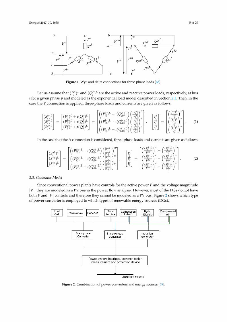
Three-phase loads can be connected in a grounded Wye (Y) configuration or an ungroundeddelta (∆) configuration as shown in Figure 1. Loads are connected phase-to-neutral or phase-to-phasein a four-wire Wye configuration. Similarly, loads are connected phase-to-phase in a three-wiredelta configuration.
Energies 2017, 10, 1658 5 of 20
Figure 1. Wye and delta connections for three-phase loads [68].
Let us assume that (Ppi )
L and (Qpi )
L are the active and reactive power loads, respectively, at busi for a given phase p and modeled as the exponential load model described in Section 2.1. Then, in thecase the Y connection is applied, three-phase loads and currents are given as follows:
(Sai )
L
(Sbi )
L
(Sci )
L
=
(Pai )
L + ı(Qai )
L
(Pbi )
L + ı(Qbi )
L
(Pci )
L + ı(Qci )
L
=
((Pa
i0)L + ı(Qa
i0)L)( |Va
i ||Va
0 |
)n((Pb
i0)L + ı(Qb
i0)L)( |Vb
i ||Vb
0 |
)n((Pc
i0)L + ı(Qc
i0)L)( |Vc
i ||Vc
0 |
)n
,
Iai
Ibi
Ici
=
((Sa
i )L
Vai
)∗((Sb
i )L
Vbi
)∗((Sc
i )L
Vci
)∗ . (1)
In the case that the ∆ connection is considered, three-phase loads and currents are given as follows:
(Sabi )L
(Sbci )L
(Scai )L
=
((Pab
i0 )L + ı(Qab
i0 )L)( |Vab
i ||Vab
0 |
)n
((Pbc
i0 )L + ı(Qbc
i0 )L)( |Vbc
i ||Vbc
0 |
)n((Pca
i0 )L + ı(Qca
i0 )L)( |Vca
i ||Vca
0 |
)n
,
Iai
Ibi
Ici
=
((Sab
i )L
Vabi
)∗−((Sca
i )L
Vcai
)∗((Sbc
i )L
Vbci
)∗−((Sab
i )L
Vabi
)∗((Sca
i )L
Vcai
)∗−((Sbc
i )L
Vbci
)∗ . (2)
2.3. Generator Model
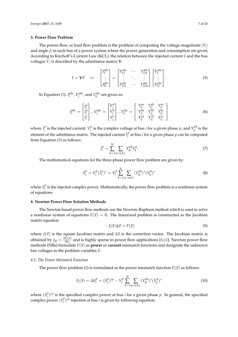
Since conventional power plants have controls for the active power P and the voltage magnitude|V|, they are modeled as a PV bus in the power flow analysis. However, most of the DGs do not haveboth P and |V| controls and therefore they cannot be modeled as a PV bus. Figure 2 shows which typeof power converter is employed to which types of renewable energy sources (DGs).
Figure 2. Combination of power converters and energy sources [69].

Energies 2017, 10, 1658 6 of 20
Depending on the types of energy sources and energy converters, the DGs are modeled as follows:
• The constant power factor model (PQ bus):The active power P output and power factor p f are specified and the reactive power Q isdetermined by these two variables.
• The variable reactive power model (PQ bus):The active power P output is specified and the reactive power Q is determined by applyinga predetermined polynomial function.
• The constant voltage model (PV bus):The active power P output and voltage magnitude |V| are specified.
The DGs modeled as PQ buses can be treated as negative PQ loads in power flow analysis.
2.4. Transformer Model
Three-phase transformers are modeled by an admittance matrix YabcT which depends upon the
connection of the primary and secondary taps, and the leakage admittance.
YabcT =
[Yabc
pp Yabcps
Yabcsp Yabc
ss
](3)
where Yabcps , Yabc
sp are a mutual admittance and Yabcpp , Yabc
ss are a self admittance of the primary andthe secondary taps, respectively. The submatrices of the admittance matrix for different transformerconnections are given in Table 2.
Table 2. Characteristic submatrices of admittance matrices for different transformer connections.
Transformer Connection Self Admittance Mutual Admittance
Bus P Bus S Yabcpp Yabc
ss Yabcps Yabc
sp
Wye-G Wye-G YI YI −YI −YIWye-G Wye YI I YI I −YI I −YI IWye-G Delta YI YI I YI I I YT
II IWye Wye-G YI I YI I −YI I −YI IWye Wye YI I YI I −YI I −YI IWye Delta YI I YI I YI I I YT
II IDelta Wye-G YI I YI YT
II I YI I IDelta Wye YI I YI I YT
II I YI I IDelta Delta YI I YI I −YI I −YI I
In this table, submatrices are given as:
YI =
yt 0 00 yt 00 0 yt
, YI I =13
2yt −yt −yt
−yt 2yt −yt
−yt −yt 2yt
, YI I I =1√3
−yt yt 00 −yt yt
yt 0 −yt
(4)
and yt is the leakage admittance of the transformer. If the transformer has an off-nominal tap ratio α:βwhere α and β are tappings on the primary and secondary sides respectively, then the submatricesmust be modified as follows:
• Divide the self admittance matrix of the primary by α2:Yabc
ppα2
• Divide the self admittance matrix of the secondary by β2: Yabcssβ2
• Divide the mutual admittance matrices by αβ:Yabc
psαβ ,
Yabcspαβ
The admittance matrix (3) for the transformer can be added to the general admittance matrixin (5). For more detailed information, we refer to [15].
Energies 2017, 10, 1658 7 of 20
3. Power Flow Problem
The power flow, or load flow problem is the problem of computing the voltage magnitude |Vi|and angle δi in each bus of a power system where the power generation and consumption are given.According to Kirchoff’s Current Law (KCL), the relation between the injected current I and the busvoltages V, is described by the admittance matrix Y:
I = YV ↔
Iabc1...
IabcN
=
Yabc11 · · · Yabc
1N...
. . ....
YabcN1 · · · Yabc
NN
Vabc
1...
VabcN
. (5)
In Equation (5), Iabci , Vabc
j , and Yabcij are given as:
Iabci =
Iai
Ibi
Ici
, Vabcj =
Vaj
Vbj
Vcj
, Yabcij =
Yaaij Yab
ij Yacij
Ybaij Ybb
ij Ybcij
Ycaij Ycb
ij Yccij
(6)
where Ipi is the injected current, Vp
i is the complex voltage at bus i for a given phase p, and Ypqij is the
element of the admittance matrix. The injected current Ipi at bus i for a given phase p can be computed
from Equation (5) as follows:
Ipi =
N
∑k=1
∑q=a,b,c
Ypqik Vq
k . (7)
The mathematical equations for the three-phase power flow problem are given by:
Spi = Vp
i (Ipi )∗ = Vp
i
N
∑k=1
∑q=a,b,c
(Ypqik )∗(Vq
k )∗ (8)
where Spi is the injected complex power. Mathematically, the power flow problem is a nonlinear system
of equations.
4. Newton Power Flow Solution Methods
The Newton based power flow methods use the Newton–Raphson method which is used to solvea nonlinear system of equations F(~x) = 0. The linearized problem is constructed as the Jacobianmatrix equation
− J(~x)∆~x = F(~x) (9)
where J(~x) is the square Jacobian matrix and ∆~x is the correction vector. The Jacobian matrix isobtained by Jik = ∂Fi(~x)
∂xkand is highly sparse in power flow applications [8,62]. Newton power flow
methods (NRs) formulate F(~x) as power or current-mismatch functions and designate the unknownbus voltages as the problem variables ~x.
4.1. The Power Mismatch Function
The power flow problem (8) is formulated as the power mismatch function F(~x) as follows:
Fi(~x) = ∆Spi = (Sp
i )sp −Vp
i
N
∑k=1
∑q=a,b,c
(Ypqik )∗(Vq
k )∗ (10)
where (Spi )
sp is the specified complex power at bus i for a given phase p. In general, the specifiedcomplex power (Sp
i )sp injection at bus i is given by following equation:

Energies 2017, 10, 1658 8 of 20
(Spi )
sp = (Spi )
G − (Spi )
L
where (Spi )
G is the specified complex power generation, whereas (Spi )
L = (Ppi )
L + ı(Qpi )
L is specifiedcomplex power load at bus i for a given phase p. Here, (Pp
i )L and (Qp
i )L can be modeled as one of the
load models described in Section 2.1.
4.2. The Current Mismatch Function
The power flow problem (8) is formulated as the current-mismatch function F(~x) as follows:
Fi(~x) = ∆Ipi =
( (Spi )
sp
Vpi
)∗−
N
∑k=1
∑q=a,b,c
Ypqik Vq
k (11)
where (Spi )
sp is the specified complex power at bus i for a given phase p.The power mismatch (10) and current mismatch (11) functions given in complex form can be
reformulated into real equations and variables using polar and Cartesian coordinates. These twomismatch functions (power and current) and three coordinates (polar, Cartesian and complex form),result in six versions of the Newton–Raphson method for the solution of power flow problems.The detailed explanations of all six versions can be found in [65]. Only the version using the currentmismatch functions in polar coordinates is explained in the following section. The remaining versionscan be derived similarly.
4.2.1. Polar Current Mismatch Version (NR-c-pol)
In this version, the current mismatch function (11) is rewritten for real and imaginary parts usingpolar coordinates as follows:
∆(Iri )
p(~x) =(Psp
i )p cos δpi + (Qsp
i )p sin δpi
|Vpi |
−N
∑k=1
∑q=a,b,c
|Vqk |(G
pqik cos δ
qk − Bpq
ik sin δqk) (12)
∆(Imi )p(~x) =
(Pspi )p sin δ
pi − (Qsp
i )p cos δpi
|Vpi |
−N
∑k=1
∑q=a,b,c
|Vqk |(G
pqik sin δ
qk + Bpq
ik cos δqk). (13)
The current mismatch function can be written in vector form as follows:
F(~x) =
∆(Ir1)
abc
...∆(Ir
N)abc
∆(Im1 )abc
...∆(Im
N)abc
(14)
where
∆(Iri )
abc =
∆(Iri )
a(~x)∆(Ir
i )b(~x)
∆(Iri )
c(~x)
, ∆(Imi )abc =
∆(Imi )a(~x)
∆(Imi )b(~x)
∆(Imi )c(~x)
(15)
and we look for the solution where the current mismatch function (14) is equal to zero:
F(~x) = 0. (16)

Energies 2017, 10, 1658 9 of 20
Application of a first-order Taylor approximation to the current mismatch function (14) results ina linear system of equations that is solved in every Newton iteration:
J(~x)∆~x = F(~x) (17)
where ∆~x is the correction and J(~x) is the Jacobian matrix of the current mismatch function. Here, theJacobian matrix is obtained by taking all first-order partial derivatives of the current mismatch functionwith respect to the voltage angles δp and magnitudes |V|p as:if i 6= k
∂∆(Iri )
p(~x)∂|Vp
k |= −(Gpp
ik cos δpk − Bpp
ik sin δpk )
∂∆(Iri )
p(~x)∂δ
pk
= |Vpk |(G
ppik sin δ
pk + Bpp
ik cos δpk )
∂∆(Imi )p(~x)
∂|Vpk |
= −(Gppik sin δ
pk + Bpp
ik cos δpk )
∂∆(Imi )p(~x)∂δ
pk
= −|Vpk |(G
ppik cos δ
pk − Bpp
ik sin δpk )
if i = k
∂∆(Iri )
p(~x)∂|Vp
i |= −(Gpp
ii cos δpi − Bpp
ii sin δpi )−
(Pspi )p cos δ
pi + (Qsp
i )p sin δpi
|Vpi |2
∂∆(Iri )
p(~x)∂δ
pi
= |Vpi |(G
ppii sin δ
pi + Bpp
ii cos δpi )−
(Pspi )p sin δ
pi − (Qsp
i )p cos δpi
|Vpi |
∂∆(Imi )p(~x)
∂|Vpi |
= −(Gppii sin δ
pi + Bpp
ii cos δpi )−
(Pspi )p sin δ
pi − (Qsp
i )p cos δpi
|Vpi |2
∂∆(Imi )p(~x)∂δ
pi
= −|Vpi |(G
ppii cos δ
pi − Bpp
ii sin δpi ) +
(Pspi )p cos δ
pi + (Qsp
i )p sin δpi
|Vpi |
The linear system of Equation (17) that is solved in every Newton iteration can be written inmatrix form as follows:
−
∂∆(Ir1)
abc
∂δabc1
· · · ∂∆(Ir1)
abc
∂δabcN
∂∆(Ir1)
abc
∂|Vabc1 |
· · · ∂∆(Ir1)
abc
∂|VabcN |
.... . .
......
. . ....
∂∆(IrN)abc
∂δabc1
· · · ∂∆(IrN)abc
∂δabcN
∂∆(IrN)abc
∂|Vabc1 |
· · · ∂∆(IrN)abc
∂|VabcN |
∂∆(Im1 )abc
∂δabc1
· · · ∂∆(Im1 )abc
∂δabcN
∂∆(Im1 )abc
∂|Vabc1 |
· · · ∂∆(Im1 )abc
∂|VabcN |
.... . .
......
. . ....
∂∆(ImN )abc
∂δabc1
· · · ∂∆(ImN )abc
∂δabcN
∂∆(ImN )abc
∂|Vabc1 |
· · · ∂∆(ImN )abc
∂|VabcN |
∆δabc1...
∆δabcN
∆|Vabc1 |...
∆|VabcN |
=
∆(Ir1)
abc
...∆(Ir
N)abc
∆(Im1 )abc
...∆(Im
N)abc
(18)
where

Energies 2017, 10, 1658 10 of 20
∆δabci =
∆δai
∆δbi
∆δci
,∂∆(Ir
i )abc
∂δabcj
=
∂∆(Ir
i )a
∂δaj
∂∆(Iri )
a
∂δbj
∂∆(Iri )
a
∂δcj
∂∆(Iri )
b
∂δaj
∂∆(Iri )
b
∂δbj
∂∆(Iri )
b
∂δcj
∂∆(Iri )
c
∂δaj
∂∆(Iri )
c
∂δbj
∂∆(Iri )
c
∂δcj
, (19)
∆|Vabci | =
∆|Vai |
∆|Vbi |
∆|Vci |
,∂∆(Im
i )abc
∂|Vabcj |
=
∂∆(Im
i )a
∂|Vaj |
∂∆(Imi )a
∂|Vbj |
∂∆(Imi )a
∂|Vcj |
∂∆(Imi )b
∂|Vaj |
∂∆(Imi )b
∂|Vbj |
∂∆(Imi )b
∂|Vcj |
∂∆(Imi )c
∂|Vaj |
∂∆(Imi )c
∂|Vbj |
∂∆(Imi )c
∂|Vcj |
. (20)
The bus voltage correction in polar coordinate is given by:
|Vpi |
(h+1) = |Vpi |
(h) + ∆|Vpi |
(h) (21)
(δpi )
(h+1) = (δpi )
(h) + ∆(δpi )
(h) (22)
where h is the iteration counter. Then the complex voltage at bus i can be computed by:
(Vpi )
(h+1) = |Vpi |
(h+1)eı(δpi )
(h+1). (23)
4.2.2. Representation of PV Buses for NR-c-pol
In case of a PV bus j, a voltage magnitude |Vabcj | is specified instead of reactive power Qabc
j where
|Vabcj | =
|Vaj ||Vb
j ||Vc
j |
, Qabcj =
Qaj
Qbj
Qcj
. (24)
In the current mismatch formulation, it is possible to choose the reactive power Qpj at the bus j for
a given phase p as an unknown variable as a voltage magnitude |V| or an angle δ. Since Qabcj is an
unknown variable, all the first-order partial derivatives ∂∆(Iri )
abc
∂Qabcj
and ∂(∆Imi )abc
∂Qabcj
must be computed as:
∂∆(Iri )
abc
∂Qabcj
=
∂∆(Ir
i )a
∂Qaj
∂∆(Iri )
a
∂Qbj
∂∆(Iri )
a
∂Qcj
∂∆(Iri )
b
∂Qaj
∂∆(Iri )
b
∂Qbj
∂∆(Iri )
b
∂Qcj
∂∆(Iri )
c
∂Qaj
∂∆(Iri )
c
∂Qbj
∂∆(Iri )
c
∂Qcj
,∂∆(Im
i )abc
∂Qabcj
=
∂∆(Im
i )a
∂Qaj
∂∆(Imi )a
∂Qbj
∂∆(Imi )a
∂Qcj
∂∆(Imi )b
∂Qaj
∂∆(Imi )b
∂Qbj
∂∆(Imi )b
∂Qcj
∂∆(Imi )c
∂Qaj
∂∆(Imi )c
∂Qbj
∂∆(Imi )c
∂Qcj
(25)
where if i 6= j
∂∆(Iri )
abc(~x)∂Qabc
j=
0 0 00 0 00 0 0
,∂∆(Im
i )abc(~x)∂Qabc
j=
0 0 00 0 00 0 0
(26)
if i = j
∂∆(Irj )
abc(~x)
∂Qabcj
=
sin δa
j|Va
j |sp 0 0
0sin δb
j
|Vbj |sp 0
0 0sin δc
j|Vc
j |sp
,∂∆(Ir
j )abc(~x)
∂Qabcj
= −
cos δa
j|Va
j |sp 0 0
0cos δb
j
|Vbj |sp 0
0 0cos δc
j|Vc
j |sp
(27)

Energies 2017, 10, 1658 11 of 20
When the derivatives ∂∆(Iri )
abc
∂Qabcj
and ∂∆(Imi )abc
∂Qabcj
are added into the Jacobian matrix J(~x), the Jacobian
matrix becomes a rectangular matrix. However, all derivatives of real ∆(Iri )
abc and reactive ∆(Imi )abc
current mismatch functions with respect to |Vabcj | cannot be taken since |Vabc
j | is not an unknown
variable. Therefore, we can remove all the ∂∆(Iri )
abc
∂|Vabcj |
and ∂∆(Imi )abc
∂|Vabcj |
from the Jacobian matrix J(~x) and
the correction ∆|Vabcj | can be replaced by ∆Qabc
j . Thus, the Jacobian matrix J(~x) is again square and
therefore we will have a unique solution. The initial reactive power (Qpj )
0 at PV bus j for a given phasep is computed as follows:
(Qpj )
0 =N
∑k=1
∑q=a,b,c
|Vpj ||V
qk |(G
pqjk sin δ
qjk − Bpq
jk cos δqjk). (28)
The reactive power is updated at each iteration use.
(Qpj )
(h+1) = (Qpj )
(h) + ∆(Qpj )
(h). (29)
The flow chart of the polar current mismatch version (NR-c-pol) is given in Figure 3.The remaining versions of the Newton power flow method (NR) such as Cartesian current mismatch(NR-c-car), complex current mismatch (NR-c-com), Cartesian power mismatch (NR-p-car), andcomplex power mismatch (NR-p-com) which are newly developed for a single-phase power flowproblem in [65], can be extended to a three-phase power flow problem analogously.
let h = 0 and ~xh =
[~δh
|~V|h]
the initial iterate
compute the current-mismatches F(~xh) using (12) and (13)
||F(~xh)||∞ ≤ ε ?
solve the correction ∆~xh =
[∆~δh
∆|~V|h]
using (18)
Stop
update iterate ~xh+1 using (21) and (22)
yes
no
h = h + 1
Figure 3. Flow chart of the polar current mismatch version.

Energies 2017, 10, 1658 12 of 20
5. Numerical Experiment
We have shown how all versions of the Newton power flow method, originally developed forsingle-phase power flow problems in [65], can be extended to three-phase power flow problems withunbalanced distribution networks. Depending on the properties of a given network, one versioncan work better than the other versions. Therefore, it is crucial to study which version is moresuitable for which kind of a power network. We use different load models, transformer connections,loading conditions, and R/X ratios in order to analyze the convergence ability and scalability ofall versions. Different loading conditions are considered by multiplying each bus’s power S by aconstant k as S = k ∗ S. Similarly, different R/X ratios are obtained by multiplying each branchresistance by a constant k as Z = k ∗ R + ıX. Finally, the performance of the solution methodsis evaluated for constant power and constant polynomial load models as defined in Section 2.1.The most widely used version using power mismatch function in polar coordinates (NR-p-pol [8]) ofthe Newton power flow method and backward–forward sweep-based algorithm (BFS [43]) are appliedfor comparison purposes.
Two balanced distribution networks (33-bus [70] and 69-bus [71]) and two unbalanced distributionnetworks (IEEE 13-bus [72] and IEEE 37-bus [72]) are used for the numerical experiment. All methodsare implemented in Matlab and the relative convergence tolerance ε is set to 10−5. The maximumnumber of iterations is set to 50. Experiments are performed on an Intel computer i5-4690 3.5 GHzCPU with four cores and 64 Gb memory, running a Debian 64-bit Linux 8.7 distribution.
5.1. Single-Phase Problems
The convergence results of all solution methods for balanced distribution networks (DCase33 [70]and DCase69 [71]) are shown in Table 3.
Table 3. Balanced distribution networks: DCase33 and DCase69.
Methods
Test Cases
DCase33 DCase69
Iter Time ||F(~x)||∞ Iter Time ||F(~x)||∞NR-p-pol [8] 3 0.0123 7.4675× 10⁻⁶ 4 0.0131 5.5875× 10⁻⁹
NR-p-car 3 0.0067 1.0433× 10⁻⁶ 3 0.0069 8.1777× 10⁻⁶
NR-p-com 6 0.0058 6.4610× 10⁻⁶ 7 0.0060 4.0138× 10⁻⁶
NR-c-pol 3 0.0087 1.4291× 10⁻⁹ 3 0.0090 8.5226× 10⁻⁹
NR-c-car 3 0.0073 1.3954× 10⁻⁹ 3 0.0077 1.9503× 10⁻⁸
NR-c-com 7 0.0068 5.3792× 10⁻⁶ 10 0.0084 2.7697× 10⁻⁶
BFS [43] 7 0.0102 1.0454× 10⁻⁶ 7 0.0104 7.7770× 10⁻⁶
From Table 3, we see that NR-c-pol and NR-c-car versions have better performance in terms ofa number of iterations and the norm of the residual of the mismatch function. Although NR-p-pol [8]and NR-p-car versions converged after the same number of iterations, the value of the residual normis larger than for the NR-c-pol and NR-c-car versions. This means that if we set the tolerance to 10−7,these versions will need extra iterations to converge, whereas NR-c-pol and NR-c-car versions stillconverge after three iterations. We also see that NR-p-com, NR-c-com and BFS [43] methods needmore iterations and have a linear convergence compared to other versions which have a quadraticconvergence. These three methods solve the power flow problem in complex form, whereas otherversions (NR-p-car, NR-p-pol, NR-c-car, and NR-c-pol) reformulate the problem into real equationsusing Cartesian and polar coordinates. Figure 4a shows the comparison of the results obtained byproposed solution methods with the well-known result of the existing method [48] for the computedvoltage magnitude of DCase69. All the results of the proposed solution methods match the well-knownresult well with accuracy of 10−5 as shown in Figure 4b.

Energies 2017, 10, 1658 13 of 20
A convergence result of all solution methods for the balanced distribution network DCase69with different loading conditions and different R/X ratios, is shown in Figures 5 and 6, respectively.We see that NR-p-com, NR-c-com, and BFS [43] are more sensitive to the change of loads and R/Xratios compared to other versions that use real variables and values for the problem formulation usingpolar and Cartesian coordinates. Figure 7 shows the convergence of all solution methods for differentload models. It is clear that for all methods, a constant power (PQ) model is more suitable to use ona balanced distribution network.
Thus, we can conclude that NR-c-pol and NR-c-car versions developed in [65] are more suitablefor balanced distribution networks than versions using power mismatch functions (NR-p-pol [8],NR-p-car). Furthermore, NR-p-com and NR-c-com versions, as well as BFS [43] are the least preferablemethods for balanced distribution networks in terms of convergence and robustness.
0 10 20 30 40 50 60 70
0.95
1
buses
|V|
NR-p-pol [8]NR-p-rec
NR-p-comNR-c-polNR-c-rec
NR-c-comBFS [43]
Method [48]
(a)
0 10 20 30 40 50 60 70
0
1
2
·10−5
buses
|V| [4
8]−|V|
NR-p-pol [8]NR-p-rec
NR-p-comNR-c-polNR-c-rec
NR-c-comBFS [43]
(b)
Figure 4. Computed voltage magnitude of DCase69. (a) Computed voltage magnitude |V|; (b) Differencebetween proposed methods and existing method [48] for the computed voltage magnitude.

Energies 2017, 10, 1658 14 of 20
NR-p-p
ol[8]
NR-p-ca
r
NR-p-co
m
NR-c-pol
NR-c-ca
r
NR-c-co
m
BFS[43]
0
10
20
30
4 37
3 3
107
4 4
11
3 3
15
94 4
21
4 4
31
12It
erat
ion
num
ber
k = 1 k = 1.5 k = 2
Figure 5. Convergence results for different loading conditions (S = k ∗ S) in DCase69.
NR-p-p
ol[8]
NR-p-ca
r
NR-p-co
m
NR-c-pol
NR-c-ca
r
NR-c-co
m
BFS[43]
0
20
40
60
4 3 7 3 310 74 4
93 3
149
4 4
27
4 4
58
14
Iter
atio
nnu
mbe
r
k = 1 k = 1.5 k = 2.5
Figure 6. Convergence results for different R/X ratios (Z = k ∗ R + ıX) in DCase69.
NR-p-p
ol[8]
NR-p-ca
r
NR-p-co
m
NR-c-pol
NR-c-ca
r
NR-c-co
m
BFS[43]
2
4
6
8
10
43
7
3 3
10
77 7 76
7
10
7
Iter
atio
nnu
mbe
r
PQ Po
Figure 7. Convergence result for different load models (constant power (PQ) and polynomial (Po))in DCase69.
5.2. Three-Phase Problems
For IEEE 13-bus (DCase13) and IEEE 37-bus (DCase37) test networks, regulators are removed andall three-phase loads are chosen to be connected in a grounded Wye configuration as defined in Section2.2. For the unbalanced distribution network DCase13, the transformer is connected in Wye-G, whereas

Energies 2017, 10, 1658 15 of 20
DCase37 has the delta–delta transformer connection as defined in Section 2.4. The BFS method [43]is not implemented for three-phase power flow problems since it is not explained in sufficient detailhow the three-phase transformer is handled for this method. The convergence result of all solutionmethods for unbalanced distribution networks (DCase13 and DCase37) is shown in Table 4.
From Table 4, we see that except for the NR-p-com and NR-c-com versions, all methods convergedafter the same number of iterations for both unbalanced distribution networks. However, NR-c-pol andNR-c-car versions have better performance in terms of both number of iterations and residual norm ofthe mismatch function, as we had the same result for balanced distribution networks. Again, NR-p-comand NR-c-com versions need more iterations to converge compared to other versions.
Table 4. Unbalanced distribution networks: DCase13 and DCase37.
Methods
Test Cases
DCase13 DCase37
Iter Time ||F(~x)||∞ Iter Time ||F(~x)||∞NR-p-pol [8] 3 0.0116 1.5571× 10⁻⁹ 2 0.0134 3.4150× 10⁻⁷
NR-p-car 3 0.0067 6.7018× 10⁻⁹ 2 0.0069 1.1627× 10⁻⁷
NR-p-com 5 0.0055 5.0957× 10⁻⁷ 3 0.0055 5.3394× 10⁻⁷
NR-c-pol 3 0.0087 6.9974× 10⁻¹¹ 2 0.0094 3.9750× 10⁻⁸
NR-c-car 3 0.0073 8.1499× 10⁻¹¹ 2 0.0079 4.0339× 10⁻⁸
NR-c-com 5 0.0067 3.5585× 10⁻⁷ 3 0.0065 7.4985× 10⁻⁷
A convergence result of all solution methods for the unbalanced distribution network DCase13with different loading conditions and different R/X ratios is shown in Figures 8 and 9, respectively.As in single-phase cases, NR-p-com and NR-c-com versions are more sensitive to the change of loadsand R/X ratios compared to other versions. Moreover, NR-c-pol and NR-c-car versions were morestable for the changes and therefore they can be applied to any unbalanced distribution networks withhigh R/X ratios and loading conditions. All methods performed better when a constant power (PQ)model was applied to three-phase problems as shown in Figure 10. We can conclude that versionsusing the current mismatch functions (NR-c-pol and NR-c-car) are more suitable than versions usingthe power-mismatch functions (NR-p-pol [8] and NR-p-car) for unbalanced distribution networks.
NR-p-p
ol[8]
NR-p-ca
r
NR-p-co
m
NR-c-pol
NR-c-ca
r
NR-c-co
m
0
10
20
30
40
3 3 5 3 3 54 4
15
4 4
15
5 5
36
4 4
37
Iter
atio
nnu
mbe
r
k = 1 k = 10 k = 20
Figure 8. Convergence results for different loading conditions (S = k ∗ S) in DCase13.

Energies 2017, 10, 1658 16 of 20
NR-p-p
ol[8]
NR-p-ca
r
NR-p-co
m
NR-c-pol
NR-c-ca
r
NR-c-co
m
5
10
15
20
3 35
3 354 4
7
3 3
86 6
19
3 4
16
Iter
atio
nnu
mbe
r
k = 1 k = 10 k = 20
Figure 9. Convergence results for different R/X ratios (Z = k ∗ R + ıX) in DCase13.
NR-p-p
ol[8]
NR-p-ca
r
NR-p-co
m
NR-c-pol
NR-c-ca
r
NR-c-co
m
3
4
5
3 3
5
3 3
5
4 4
5
4 4
5
Iter
atio
nnu
mbe
r
PQ Po
Figure 10. Convergence result for different load models (constant power (PQ) and polynomial (Po))in DCase13.
6. Conclusions
In this paper, the Newton power flow methods developed for single-phase problems in [65]are extended to three-phase power flow problems. Mathematical models of the load, three-phaseload connection, and three-phase transformer connection are studied and applied in the numericalexperiments. The power flow problem is mathematically described for the three-phase problem.The Newton power flow method and its six possible versions are introduced for three-phase powerflow problems. As one of the newly developed versions of the Newton power flow method, the polarcurrent mismatch version (NR-c-pol) is explained in detail for a three-phase power flow problem.The existing version (NR-p-pol [8]) and the backward–forward sweep-based algorithm (BFS [43]) areapplied for comparison purposes. As a result of the numerical experiment, the polar current mismatch(NR-c-pol) and the Cartesian current mismatch (NR-c-car) versions developed in [65] and extendedin this paper perform the best for both balanced and unbalanced distribution networks. We alsoinvestigate which version can be applied to what kind of a power network by comparing all versionsfor distribution networks with different loading conditions, R/X ratios, and load models. We observethat NR-c-pol and NR-c-car versions are more stable to the change of loading conditions and R/Xratios for both balanced and unbalanced networks, whereas the performance of other methods ishighly sensitive to them. Therefore, these two versions are the fastest and the most robust methods ofother versions that can be applied to single or three-phase power flow problems in any balanced orunbalanced networks. For the subsequent research, these newly developed versions (NR-c-pol and

Energies 2017, 10, 1658 17 of 20
NR-c-car) will be applied to the optimal power flow problem in hybrid networks including DGs asthey result in new formulations for equality constraints.
Acknowledgments: This research is supported by the Netherlands Organization for Scientific Research Science(NWO), domain Applied and Engineering Sciences, Grant No. 14181.
Author Contributions: All the authors contributed equally in all aspects of this work.
Conflicts of Interest: The authors declare no conflict of interest.
Abbreviations
The following abbreviations are used in this manuscript:
BFS backward-forward sweepDG distributed generationDSO distribution system operatorsFDLF fast-decoupled load flowGS Gauss–SeidelNR Newton power flow methodNR-p-pol polar power mismatch version of NRNR-p-car Cartesian power mismatch version of NRNR-p-com complex power mismatch version of NRNR-c-pol polar current mismatch version of NRNR-c-car Cartesian current mismatch version of NRNR-c-com complex current mismatch version of NRTSO transmission system operatorSG smart grid
References
1. Schavemaker, P.; van der Sluis, L. Electrical Power System Essentials; Wiley: Hoboken, NJ, USA, 2008.2. Keyhani, A.; Marwali, M. Smart Power Grids 2011; Power Systems; Springer: Berlin, Germany, 2012.3. Budka, K.; Deshpande, J.; Thottan, M. Communication Networks for Smart Grids: Making Smart Grid Real;
Computer Communications and Networks; Springer: Berlin, Germany, 2014.4. Thomas, M.; McDonald, J. Power System SCADA and Smart Grids; Taylor & Francis: Abingdon, UK, 2015.5. Balamurugan, K.; Srinivasan, D. Review of power flow studies on distribution network with distributed
generation. In Proceedings of the 2011 IEEE Ninth International Conference on Power Electronics and DriveSystems, Singapore, 5–8 December 2011; pp. 411–417.
6. Martinez, J.A.; Mahseredjian, J. Load flow calculations in distribution systems with distributed resources.A review. In Proceedings of the 2011 IEEE Power and Energy Society General Meeting, Detroit, MI, USA,24–29 July 2011; pp. 1–8.
7. Stevenson, W.D. Elements of Power System Analysis; McGraw-Hill: New York, NY, USA, 1975.8. Tinney, W.F.; Hart, C.E. Power flow solution by Newton’s method. IEEE Trans. Power Appar. Syst.
1967, PAS-86, 1449–1460.9. Stott, B.; Alsaç, O. Fast decoupled load flow. IEEE Trans. Power Appar. Syst. 1974, PAS-93, 859–869.10. Iwamoto, S.; Tamura, Y. A load flow calculation method for Ill-conditioned power systems. IEEE Trans.
Power Appar. Syst. 1981, PAS-100, 1736–1743.11. Tripathy, S.C.; Prasad, G.D.; Malik, O.P.; Hope, G.S. Load-flow solutions for ill-conditioned power systems
by a newton-like method. IEEE Trans. Power Appar. Syst. 1982, PAS-101, 3648–3657.12. Reddy, S.; Suresh, S.S.K.; Kumar, S.V.J. Load flow solution for ill-conditioned power systems using
runge-kutta and Iwamoto methods with facts devices. J. Theor. Appl. Inf. Technol. 2009, 5, 693–703.13. Chiang, H.D. A decoupled load flow method for distribution power networks: Algorithms, analysis and
convergence study. Int. J. Electr. Power Energy Syst. 1991, 13, 130–138.14. Chen, T.H.; Chen, M.S.; Hwang, K.J.; Kotas, P.; Chebli, E.A. Distribution system power flow analysis—
A rigid approach. IEEE Trans. Power Deliv. 1991, 6, 1146–1152.15. Chen, T.H.; Chen, M.S.; Inoue, T.; Kotas, P.; Chebli, E.A. Three-phase cogenerator and transformer models
for distribution system analysis. IEEE Trans. Power Deliv. 1991, 6, 1671–1681.

Energies 2017, 10, 1658 18 of 20
16. Zhang, F.; Cheng, C.S. A modified Newton method for radial distribution system power flow analysis.IEEE Trans. Power Syst. 1997, 12, 389–397.
17. Nguyen, H.L. Newton-Raphson method in complex form. IEEE Trans. Power Deliv. 1997, 12, 1355–1359.18. Da Costa, V.M.; Martins, N.; Pereira, J.L.R. Developments in the Newton Raphson power flow formulation
based on current injections. IEEE Trans. Power Syst. 1999, 14, 1320–1326.19. Garcia, P.A.N.; Pereira, J.L.R.; Carneiro, S.; da Costa, V.M.; Martins, N. Three-phase power flow calculations
using the current injection method. IEEE Trans. Power Syst. 2000, 15, 508–514.20. Lin, W.M.; Teng, J.H. Three-phase distribution network fast-decoupled power flow solutions. Int. J. Electr.
Power Energy Syst. 2000, 22, 375–380.21. Teng, J.H.; Chang, C.Y. A novel and fast three-phase load flow for unbalanced radial distribution systems.
IEEE Trans. Power Deliv. 2002, 17, 1238–1244.22. Teng, J.H. A modified Gauss-Seidel algorithm of three-phase power flow analysis in distribution networks.
Int. J. Electr. Power Energy Syst. 2002, 24, 97–102.23. Vieira, J.; Freitas, W.; Morelato, A. Phase-decoupled method for three-phase power-flow analysis of
unbalanced distribution systems. IEE Proc. Gener. Transm. Distrib. 2004, 151, 568–574.24. Chen, T.H.; Yang, N.C. Loop frame of reference based three-phase power flow for unbalanced radial
distribution systems. Electr. Power Syst. Res. 2010, 80, 799–806.25. Sun, H.; Nikovski, D.; Ohno, T.; Takano, T.; Kojima, Y. A fast and robust load flow method for distribution
systems with distributed generations. Energy Procedia 2011, 12, 236–244.26. Lagace, P.J. Power flow methods for improving convergence. In Proceedings of the IECON 2012—38th
Annual Conference on IEEE Industrial Electronics Society, Montreal, QC, Canada, 25–28 October 2012;pp. 1387–1392.
27. Abdelaziz, M.M.A.; Farag, H.E.; El-Saadany, E.F.; Mohamed, Y.A.R.I. A novel and generalized three-phasepower flow algorithm for islanded microgrids using a Newton trust region method. IEEE Trans. Power Syst.2013, 28, 190–201.
28. Idema, R.; Lahaye, D. Computational Methods in Power System Analysis; Atlantis Studies in ScientificComputing in Electromagnetics; Atlantis Press: Amsterdam, The Netherlands, 2014.
29. Li, C.; Chaudhary, S.K.; Vasquez, J.C.; Guerrero, J.M. Power flow analysis algorithm for islanded LV microgridsincluding distributed generator units with droop control and virtual impedance loop. In Proceedings of the2014 IEEE Applied Power Electronics Conference and Exposition, Fort Worth, TX, USA, 16–20 March 2014;pp. 3181–3185.
30. Wang, L.; Chen, C.; Shen, T. Improvement of power flow calculation with optimization factor based oncurrent injection method. Discrete Dyn. Nat. Soc. 2014, 2014, 437567.
31. Milano, F. Analogy and convergence of Levenberg’s and Lyapunov-based methods for power flow analysis.IEEE Trans. Power Syst. 2016, 31, 1663–1664.
32. Mumtaz, F.; Syed, M.; Al Hosani, M.; Zeineldin, H. A novel approach to solve power flow for islandedmicrogrids using modified Newton-Raphson with droop control of DG. IEEE Trans. Sustain. Energy 2016, 7,493–503.
33. Pourbagher, R.; Derakhshandeh, S.Y. A powerful method for solving the power flow problem in theill-conditioned systems. Int. J. Electr. Power Energy Syst. 2018, 94, 88–96.
34. Cheng, C.S.; Shirmohammadi, D. A three-phase power flow method for real-time distribution systemanalysis. IEEE Trans. Power Deliv. 1995, 10, 671–679.
35. Thukaram, D.; Banda, H.W.; Jerome, J. A robust three phase power flow algorithm for radial distributionsystems. Electr. Power Syst. Res. 1999, 50, 227–236.
36. Ranjan, R.; Venkatesh, B.; Chaturvedi, A.; Das, D. Power flow solution of three-phase unbalanced radialdistribution network. Electr. Power Compon. Syst. 2004, 32, 421–433.
37. Khushalani, S.; Solanki, J.M.; Schulz, N.N. Development of three-phase unbalanced power flow using PVand PQ models for distributed generation and study of the impact of DG models. IEEE Trans. Power Deliv.2007, 22, 1019–1025.
38. Moghaddas-Tafreshi, S.; Mashhour, E. Distributed generation modeling for power flow studies anda three-phase unbalanced power flow solution for radial distribution systems considering distributedgeneration. Electr. Power Syst. Res. 2009, 79, 680–686.

Energies 2017, 10, 1658 19 of 20
39. Shirmohammadi, D.; Hong, H.; Semlyen, A.; Luo, G. A compensation-based power flow method for weaklymeshed distribution and transmission networks. IEEE Trans. Power Deliv. 1988, 3, 753–762.
40. Luo, G.X.; Semlyen, A. Efficient load flow for large weakly meshed networks. IEEE Trans. Power Syst. 1990,5, 1309–1316.
41. Haque, M.H. Efficient load flow method for distribution systems with radial or mesh configuration. IEE Proc.Gener. Transm. Distrib. 1996, 143, 33–38.
42. Haque, M. A general load flow method for distribution systems. Electr. Power Syst. Res. 2000, 54, 47–54.43. Teng, J.H. A direct approach for distribution system load flow solutions. IEEE Trans. Power Deliv. 2003, 18,
882–887.44. Rajicic, D.; Ackovski, R.; Taleski, R. Voltage correction power flow. IEEE Trans. Power Deliv. 1994, 9, 1056–1062.45. Zhu, Y.; Tomsovic, K. Adaptive power flow method for distribution systems with dispersed generation.
IEEE Trans. Power Deliv. 2002, 17, 822–827.46. Teng, J.H. Modelling distributed generations in three-phase distribution load flow. IET Proc. Gener.
Transm. Distrib. 2008, 2, 330–340.47. Augugliaro, A.; Dusonchet, L.; Favuzza, S.; Ippolito, M.; Sanseverino, E.R. A new backward/forward
method for solving radial distribution networks with PV nodes. Electr. Power Syst. Res. 2008, 78, 330–336.48. Ghosh, S.; Das, D. Method for load-flow solution of radial distribution networks. IEE Proc. Gener.
Transm. Distrib. 1999, 146, 641–648.49. Samuel Mok, S.; Elangovan, C.L.; Salama, M. A new approach for power flow analysis of balanced radial
distribution systems. Electr. Mach. Power Syst. 2000, 28, 325–340.50. Aravindhababu, P.; Ganapathy, S.; Nayar, K. A novel technique for the analysis of radial distribution systems.
Int. J. Electr. Power Energy Syst. 2001, 23, 167–171.51. Liu, J.; Salama, M.; Mansour, R. An efficient power flow algorithm for distribution systems with polynomial
load. Int. J. Electr. Eng. Educ. 2002, 39, 371–386.52. Cespedes, R. New method for the analysis of distribution networks. IEEE Trans. Power Deliv. 1990, 5, 391–396.53. Jasmon, G.; Lee, L. Distribution network reduction for voltage stability analysis and loadflow calculations.
Int. J. Electr. Power Energy Syst. 1991, 13, 9–13.54. Das, D.; Nagi, H.; Kothari, D. Novel method for solving radial distribution networks. IEE Proc. Gener.
Transm. Distrib. 1994, 141, 291–298.55. Das, D.; Kothari, D.; Kalam, A. Simple and efficient method for load flow solution of radial distribution
networks. Int. J. Electr. Power Energy Syst. 1995, 17, 335–346.56. Haque, M. Load flow solution of distribution systems with voltage dependent load models. Electr. Power
Syst. Res. 1996, 36, 151–156.57. Afsari, M.; Singh, S.; Raju, G.; Rao, G. A fast power flow solution of radial distribution networks. Electr. Power
Compon. Syst. 2002, 30, 1065–1074.58. Mekhamer, S.; Soliman, S.; Moustafa, M.; El-Hawary, M. Load flow solution of radial distribution feeders:
A new contribution. Int. J. Electr. Power Energy Syst. 2002, 24, 701–707.59. Ranjan, R.; DAS. Simple and efficient computer algorithm to solve radial distribution networks. Electr. Power
Compon. Syst. 2003, 31, 95–107.60. Eminoglu, U.; Hocaoglu, M.H. A new power flow method for radial distribution systems including voltage
dependent load models. Electr. Power Syst. Res. 2005, 76, 106–114.61. Satyanarayana, S.; Ramana, T.; Sivanagaraju, S.; Rao, G. An efficient load flow solution for radial distribution
network including voltage dependent load models. Electr. Power Compon. Syst. 2007, 35, 539–551.62. Stott, B. Review of load-flow calculation methods. Proc. IEEE 1974, 62, 916–929.63. Srinivas, M.S. Distribution load flows: A brief review. In Proceedings of the 2000 IEEE Power Engineering
Society Winter Meeting, Singapore, 23–27 January 2000; Volume 2, pp. 942–945.64. Eminoglu, U.; Hocaoglu, M.H. Distribution systems forward/backward sweep-based power flow algorithms:
A review and comparison study. Electr. Power Compon. Syst. 2008, 37, 91–110.65. Sereeter, B.; Vuik, C.; Witteveen, C. On a Comparison of Newton-Raphson Solvers for Power Flow Problems; Report
17-7; Delft Institute of Applied Mathematics, Delft University of Technology: Delft, The Netherlands, 2017.66. Van Ness, J.E.; Griffin, J.H. Elimination methods for load-flow studies. Trans. Am. Inst. Electr. Eng. Part III
1961, 80, 299–302.

Energies 2017, 10, 1658 20 of 20
67. Lindén, K.; Segerqvist, I. Modelling of Load Devices and Studying Load/System Characteristics; Technical Report;Chalmers University of Technology: Gothenburg, Sweden, 1992.
68. Subrahmanyam, J.; Radhakrishna, C. A simple approach of three phase distribution system modeling forpower flow calculations. Int. J. Energy Power Eng. 2010, 3, 3.
69. Electric Power Research Institute (EPRI). Engineering Guide for Integration of Distributed Generation and Storageinto Power Distribution Systems; Technical Report; EPRI: Palo Alto, CA, USA, 2000.
70. Baran, M.E.; Wu, F.F. Network reconfiguration in distribution systems for loss reduction and load balancing.IEEE Trans. Power Deliv. 1989, 4, 1401–1407.
71. Baran, M.E.; Wu, F.F. Optimal capacitor placement on radial distribution systems. IEEE Trans. Power Deliv.1989, 4, 725–734.
72. Kersting, W.H. Radial distribution test feeders. In Proceedings of the 2001 IEEE Power Engineering SocietyWinter Meeting, Columbus, OH, USA, 28 January–1 February 2001; Volume 2, pp. 908–912.
c© 2017 by the authors. Licensee MDPI, Basel, Switzerland. This article is an open accessarticle distributed under the terms and conditions of the Creative Commons Attribution(CC BY) license (http://creativecommons.org/licenses/by/4.0/).