Newtonian Particles

Steve RotenbergCSE291: Physics Simulation

UCSDSpring 2019

CSE291: Physics Simulation

• Instructor: Steve Rotenberg (srotenberg@ucsd.edu)

• Lecture: EBU3 4140 (TTh 5:00 – 6:20pm)

• Office: EBU3 2210 (TTh 3:50– 4:50pm)

• TA: Mridul Kavidayal (mkaviday@eng.ucsd.edu)

• Web page:

https://cseweb.ucsd.edu/classes/sp19/cse291-d/index.html

CSE291: Physics Simulation

• Focus will be on physics of motion (dynamics)

• Main subjects:– Solid mechanics (deformable bodies & fracture)

– Fluid dynamics

– Rigid body dynamics

• Additional topics:– Vehicle dynamics

– Galactic dynamics

– Molecular modeling

Programming Project

• There will a single programming project over the quarter• You can choose one of the following options

– Fracture modeling– Particle based fluids– Rigid body dynamics

• Or you can suggest your own idea, but talk to me first• The project will involve implementing the physics, some level of

collision detection and optimization, some level of visualization, and some level of user interaction

• You can work on your own or in a group of two• You also have to do a presentation for the final and demo it live or

show some rendered video• I will provide more details on the web page

Grading

• There will be two pop quizzes, each worth 5% of the total grade

• For the project, you will have to demonstrate your current progress at two different times in the quarter (roughly 1/3 and 2/3 through). These will each be worth 10% of the total grade

• The final presentation is worth 10%

• The remaining 60% is for the content of the project itself

Course Outline

1. Newtonian Particles2. Integration3. Elasticity4. Finite Elements5. Mesh Generation6. Contact Modeling7. Fracture8. Vector Calculus9. Fluid Dynamics

10.Poisson Equations11.Particle-Based Fluids12.Advanced Fluids13.Rigid Body Motion14.Articulated Bodies15.Rigid Body Collisions16.Vehicle Dynamics17.Galactic Dynamics18.Molecular Modeling

Recommended Reading

• “Nonlinear Finite Elements for Continua and Structures”, Second Edition

• Belytschko, Liu, Moran, Elkhodary, 2014

• In addition, I will post several papers on the web page

Physics Resources

• “Numerical Recipes: The Art of Scientific Computing, 3rd

Edition” is also a great book that covers a wide range of useful numerical techniques (Press, Teukolsky, Vetterling, Flannery, 2007)

• www.PhysicsBasedAnimation.com is a great web page with links to tons of papers on advanced physics simulation

• “An Introduction to Physics-based Animation” was a course at SIGGRAPH 2018 presented by Adam Bargteil and Tamar Shinar

http://www.cs.ucr.edu/~shinar/papers/2018_introduction_to_pba.pdf

Simulation & Models

Simulation

• A simulation is an imitation of a process based on a model (or model equations) and using approximation

• The model represents the system being simulated

• The simulation represents the behavior of the system over time

• Simulation can be applied to natural systems such as chemistry, biology, and physics, or human systems such as economics, social science, transportation

• Powerful tool in research, engineering, education, training, entertainment…

Models

• The model is a set of equations that describes the behavior of the system over time

• Models of physical systems always involve some level of approximation (for example, we can model a ball bouncing without having to model the quantum mechanics of every single subatomic particle in the ball)

• Models can be discreet or continuous in time• In a continuous simulation, the model equations are typically

differential equations that are based on physics• One can also perform discrete simulations (such as a logic

simulation of a computer chip) that are based on logical equations rather than differential equations

• We will focus mainly on time continuous simulations in this class

Model Validation

• Often times, simulations are used to predict the behavior of some real world process

• In this case, the simulation is only useful if can match the real world to some degree of accuracy

• Simulation models can be directly compared to real world measurements to verify the validity of the model and determine the range of parameters where the simulation is useful

Model Calibration

• Often, models can be calibrated to match real world results• If a particular model has adjustable constants, then one can

use calibration algorithms that can set these constants such as to optimize a models ability to reproduce a set of real world results

• For example, if we have a simulation of a cannon ball and we want to predict how far it will fly, we have some constants that we don’t want to mess with (such as gravity, or the radius of the cannon ball) but we might have other constants that are a little more flexible (such as the drag coefficient of the ball)

• We will come back to this in a later lecture

Degrees of Freedom

• The parameters that describe the state of the simulation are called the degrees of freedom (DOFs) of the system

• The number of DOFs is often constant, but does not have to be. For example, a simulation of fracture may result in more DOFs at the end of the simulation than at the beginning

• Simulations that use adaptive level of detail will add or remove DOFs as the simulation proceeds

• In our physics simulations, the DOFs will mainly be position and velocity values (including angles and angular velocities)

Initial Conditions

• Time-continuous simulations start at some time t0 and advance forward to some final time tfinal

• We will need to specify the initial conditions, which requires values for all of the DOFs at time t0

• For some simulations, specifying the model and the initial conditions is enough to determine the entire simulation

• For other simulations (such as interactive, or human-in-the-loop), there will also be a continuous stream of input data that is generated throughout the simulation

Visualization

• There is a lot to be said about visualization of physics simulations, but the details are outside of the scope of this class

• We can at least assume that we will want to draw the objects we are simulating in some sort of animation

• In addition to the object geometry, we can also visualize forces, velocities, pressures, temperature, stresses, and any other properties we are interested in

• We will assume the use of OpenGL or some similar graphics API for this class, and stick to fairly simple visualization

Physical Domains

Physical Domains

• Depending on what we’re simulating, we may operate in different physical domains

Slow to fast Very fast

Small to very large size

Classical Relativistic

Very small Quantum Mechanical

Quantum Field Theory

Classical Domain

• The classical domain refers to the physics of everyday objects from things as small as a molecule to as large as a cluster of galaxies

• We can divide the classical domain further into:– Mechanics

– Electromagnetics

– Statistical Mechanics

– Thermodynamics

– And more…

• In this course, we will mostly be interested in classical mechanics, but we will touch on some other areas

Quantum Domain

• If we want to model very small things down at the level of electrons, we need to work in the domain of quantum mechanics

• Quantum mechanical simulations are typically based on the Schrödinger Equation, in either the time-dependent or time-independent form

• With these models, we can predict shapes of molecules as well as their chemical properties based on first principles of quantum mechanics

• We will briefly discuss these in a later lecture on molecular simulation

Relativistic Domain

• If we are dealing with very fast moving objects near the speed of light, we operate in the domain of relativistic mechanics

• We can model systems based on both special relativity or general relativity

• For example, simulations of black hole merging are done using space-time general relativistic models

Quantum Field Theory Domain

• If we need both high relativistic speeds and small quantum scales, we can work in the domain of quantum field theory

• This is used for simulations of subatomic particle interactions and modeling of the Standard Model of elementary particles and the fundamental forces of nature

• Unfortunately, we won’t be covering this…

Classical Mechanics

Statics vs. Dynamics

• The field of classical mechanics includes both statics and dynamics• Statics refers to the analysis of stable configurations for things such

as structures (buildings, bridges…). This can also apply to steady-state motion such as an aircraft cruising at a constant speed.

• Dynamics refers to the study of change. This often refers to physical movement, but can also refer to changes in other properties such as temperature as in thermodynamics.

• Within dynamics we sometimes refer to modal dynamics as the study of repeating oscillations in the frequency domain vs. transient dynamics as the study of non-repeating processes in the time domain.

• In this course, we will mainly be interested in transient dynamics, but will occasionally discuss statics and modal dynamics.

Kinematics

• The subject of mechanics also includes kinematics which is the geometric description of motion, independent of the physical forces involved

• Kinematics describes motion in terms of positions, velocities, and accelerations, but makes no reference to the causes of the motions (i.e., forces, masses, momentum…)

Newtonian Dynamics

• Within the realm of classical mechanics, there are several ways to formulate equations of motion

• Newtonian formulations are based around the use of Newton’s Second Law: f=ma

• One typically starts by computing all of the forces, acting on all of the degrees of freedom in a system, usually in a single global frame of reference

• These physical forces can then be related to kinematic accelerations using f=ma

• The accelerations can then be integrated to produce velocities and positions

• The Newtonian formulation of dynamics is particularly well suited to geometrically complex transient dynamic problems, such as the ones we are interested in

• Most of the systems we discuss in this course will be based on this type of formulation

Lagrangian Dynamics

• In 1788, Joseph-Louis Lagrange reformulated classical mechanics into a system now known as Lagrangian mechanics

• Lagrangian mechanics applies to systems with constraints• Typically these constraints are described geometrically, for example, one

might describe the motion of a door that is constrained by a hinge• The Newtonian formulation would think of a door as a 6 degree-of-

freedom (DOF) rigid body that is constrained in 5 of its DOFs. This leads to 5 unknown constraint forces that need to be solved, which can be costly

• The Lagrangian formulation defines a set of generalized DOFs that express only the unconstrained motion. In the case of a door, it would require only 1 DOF

• In highly constrained situations, Lagrangian formulations often reduce to simpler sets of equations than Newtonian ones, and can be more efficient to compute

• We will look at these in more detail when we discuss articulated rigid bodies in a later lecture

Hamiltonian Dynamics

• In 1833, William Rowan Hamilton reformulated classical mechanics once again, starting with Lagrangian mechanics

• It is similar to Lagrangian dynamics in that it uses generalized coordinates and formulates the equations in terms of energy

• It is more abstract than the Newtonian approach but can be useful for understanding the behavior of complex systems with many degrees of freedom

• We will briefly cover this method in a later lecture

Newtonian Particles

Kinematics of Particles

• We will define an individual particle’s 3D position over time as r(t), or just r

• By definition, velocity is the first derivative of position:

𝐯 𝑡 =𝑑𝐫

𝑑𝑡

• And acceleration is the second derivative:

𝐚 𝑡 =𝑑𝐯

𝑑𝑡=

𝑑2𝐫

𝑑𝑡2

Uniform Acceleration

• How does a particle move when undergoing a constant acceleration?

𝐚 𝑡 = 𝐚0

𝐯 𝑡 = 𝐚𝑑𝑡 = 𝐯0 + 𝐚0𝑡

𝐫 𝑡 = 𝐯𝑑𝑡 = 𝐫0 + 𝐯0𝑡 +1

2𝐚0𝑡

2

Uniform Acceleration

𝐫 𝑡 = 𝐫0 + 𝐯0𝑡 +1

2𝐚0𝑡

2

• This shows us that a particle undergoing a constant acceleration will follow a parabola

• Keep in mind that this is a 3D vector equation and there is potentially a parabola equation in each dimension. Together, they will form a 2D parabola oriented in 3D space

• We also see that we need two additional vectors 𝐫0and 𝐯0 in order to fully specify the equation. These represent the initial position and velocity at time t=0

Newton’s First Law

• Newton’s First Law states that a body in motion will remain in motion and a body at rest will remain at rest- unless acted upon by some force

• This implies that a free particle moving out in space will just travel in a straight line:

𝐚 = 0

𝐯 = 𝐯0𝐫 = 𝐫0 + 𝐯0𝑡

Mass and Momentum

• We can associate a mass m with each particle. We will assume that the mass is constant:

𝑚 = 𝑚0

• We will also define a vector quantity called momentum p, which is the product of scalar mass and vector velocity

𝐩 = 𝑚𝐯

Force

• Force is defined as the rate of change of momentum

𝐟 =𝑑𝐩

𝑑𝑡• If we assume that mass m is constant, we can expand

this to:

𝐟 =𝑑𝐩

𝑑𝑡=𝑑 𝑚𝐯

𝑑𝑡= 𝑚

𝑑𝐯

𝑑𝑡= 𝑚𝐚

𝐟 = 𝑚𝐚

Newton’s Second Law

• Newton’s Second Law says:

𝐟 =𝑑𝐩

𝑑𝑡= 𝑚𝐚

• This relates the kinematic quantity of acceleration a to the physical quantity of force f

Newton’s Third Law

• Newton’s Third Law says that any force that body A applies to body B will be met by an equal and opposite force from B to A

𝐟𝐴𝐵 = −𝐟𝐵𝐴

• Put another way: every action has an equal and opposite reaction

• This is very important when combined with the Second Law, as the two together imply the Law of Conservation of Momentum

Conservation of Momentum

• Remember that a force is a rate of change of momentum

• If Newton’s Third Law says that the forces in a system cancel out, then the total change of momentum of the system must be 0

• Therefore, the total momentum in a system must remain constant

• This is the Law of Conservation of Momentum

Forces on a Particle

• A particle may be subjected to several simultaneous vector forces from different sources

• All of these forces simply add up to a single total force acting on the particle:

𝐟𝑡𝑜𝑡𝑎𝑙 =𝐟𝑖

Newtonian Mechanics

• Newton’s Second Law relates the property of force to the kinematic property of acceleration through a measureable constant mass:

𝐟 = 𝑚𝐚• Forces are a very useful property to work with because of Newton’s

Third Law:𝐟𝐴𝐵 = −𝐟𝐵𝐴

• And because they add up in a very simple way:

𝐟𝑡𝑜𝑡𝑎𝑙 =𝐟𝑖

• These principles form the foundation of all Newtonian based simulations, including solid dynamics, rigid body dynamics, and fluid dynamics

Differential Equations

• The forces in a system are generally based on the current configuration of the system

• Mathematically, this says that the second derivative (acceleration) of a value is dependent on the value itself (and possibly it’s first derivative as well)

• This implies that the equations of motion will be differential equations (as the equations contain differentials…)

• In particular, they will be second order ordinary differential equations

• Ultimately, we wish to integrate these to compute positions over some time range

Integration

• Newton’s Second Law (f=ma) relates the physical forces in a system to the kinematic accelerations

• Given initial conditions (initial positions and velocities), we can integrate the accelerations to compute the velocities and positions over time

• In practice, we won’t be able to compute an exact integral because the system is too complicated and produces equations that might not have exact integrals

• We therefore have to resort to a numerical integration technique, where we rely on some degree of approximation

Numerical Integration

• There are many techniques to numerically integrate systems of ordinary differential equations

• They differ in computational cost, accuracy, stability, and flexibility

• We will spend the next lecture examining them in more detail

• For today, we will stick to the simplest method, known as the forward Euler method

Forward Euler Integration

• The forward Euler method uses the derivative at the start of the time step to advance the simulation forward

• For example, to compute the new velocity at time step i+1, we use the acceleration computed at time step i and assume it holds constant for the duration of ∆𝑡

𝐯𝑖+1 = 𝐯𝑖 + 𝐚𝑖∆𝑡

• For the position integration, we do essentially the same thing, except we use the new velocity instead of the previous velocity

𝐫𝑖+1 = 𝐫𝑖 + 𝐯𝑖+1∆𝑡

• We will discuss this further in the next lecture…

Newtonian Simulation

• Newtonian simulations generally follow a pattern like this:

- Set up initial conditions- while (not finished) {

- Compute all forces in the system, which can then be used to compute the accelerations through f=ma- Integrate the accelerations one small step forward in time to compute new velocities and positions

}

• Sure, the details will get more complicated, but in general, we are taking finite steps forward in time and evaluating forces at each step

Particle Example

class Particle {public:

void ApplyForce(vec3 &f) {Force+=f;}void Integrate(float deltaTime) {

vec3 accel=(1/Mass) * Force;Velocity += accel*deltaTime;Position += Velocity*deltaTime;Force=vec3(0);

}private:

vec3 Position;vec3 Velocity;vec3 Force;float Mass;

};

Energy

• The kinetic energy of a particle is 1

2𝑚 𝐯 2

• There are also various forms of potential energy such (gravity, springs, etc. can store energy as a potential)

• Energy in a system may convert between different forms (kinetic, potential, thermal, electromagnetic…) but the total energy in a system remains constant

• The subject of energy is important in physics, but Newtonian formulations of the equations rarely make direct use of it

• We will therefore not discuss it much today, but it will come back from time to time in later lectures

Basic Forces

Uniform Gravity

• A very simple, useful force is the uniform gravity field:

𝐟𝑔𝑟𝑎𝑣𝑖𝑡𝑦 = 𝑚𝐠0

𝐠0 = 0 −9.8 0𝑚

𝑠2

• It assumes that we are near the surface of the Earth and we can approximate the gravity as constant in both magnitude and direction

• 9.8 m/s2 is a reasonable approximation, as it actually ranges from roughly 9.76 to 9.83 around the world due to variations in altitude and local density

• By definition, standard gravity is 9.80665 m/s2, which is a number agreed upon in 1901 and is used in various standards of weight and mass, and would make a good choice as a default gravity value for simulations

• There also exist detailed maps of Earth’s gravity that account for variation in direction and magnitude of the local gravity vector at the surface

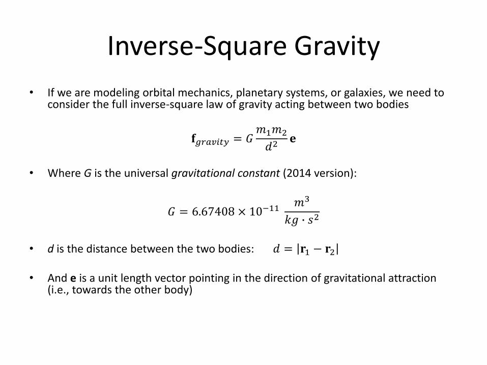
Inverse-Square Gravity

• If we are modeling orbital mechanics, planetary systems, or galaxies, we need to consider the full inverse-square law of gravity acting between two bodies

𝐟𝑔𝑟𝑎𝑣𝑖𝑡𝑦 = 𝐺𝑚1𝑚2

𝑑2𝐞

• Where G is the universal gravitational constant (2014 version):

𝐺 = 6.67408 × 10−11𝑚3

𝑘𝑔 ∙ 𝑠2

• d is the distance between the two bodies: 𝑑 = 𝐫1 − 𝐫2

• And e is a unit length vector pointing in the direction of gravitational attraction (i.e., towards the other body)

Inverse-Square Gravity

𝐟𝑔𝑟𝑎𝑣𝑖𝑡𝑦 = 𝐺𝑚1𝑚2

𝑑2𝐞

• We need to consider the gravitational force acting on every pair of bodies• In a system of n bodies, this means we need to compute a gravitational

force Τ𝑛 𝑛 − 1 2 times• In terms of algorithm performance, this implies O(n2) performance, which

is potentially slow for large values of n• It turns out that for galactic simulations with millions of particles, we can

actually achieve O(n log n) performance using some octree techniques• For big-bang simulations in periodic domains with billions of particles, we

can even achieve O(n) performance using some Fourier techniques• We will discuss these techniques in more detail in a later lecture

Aerodynamic Drag

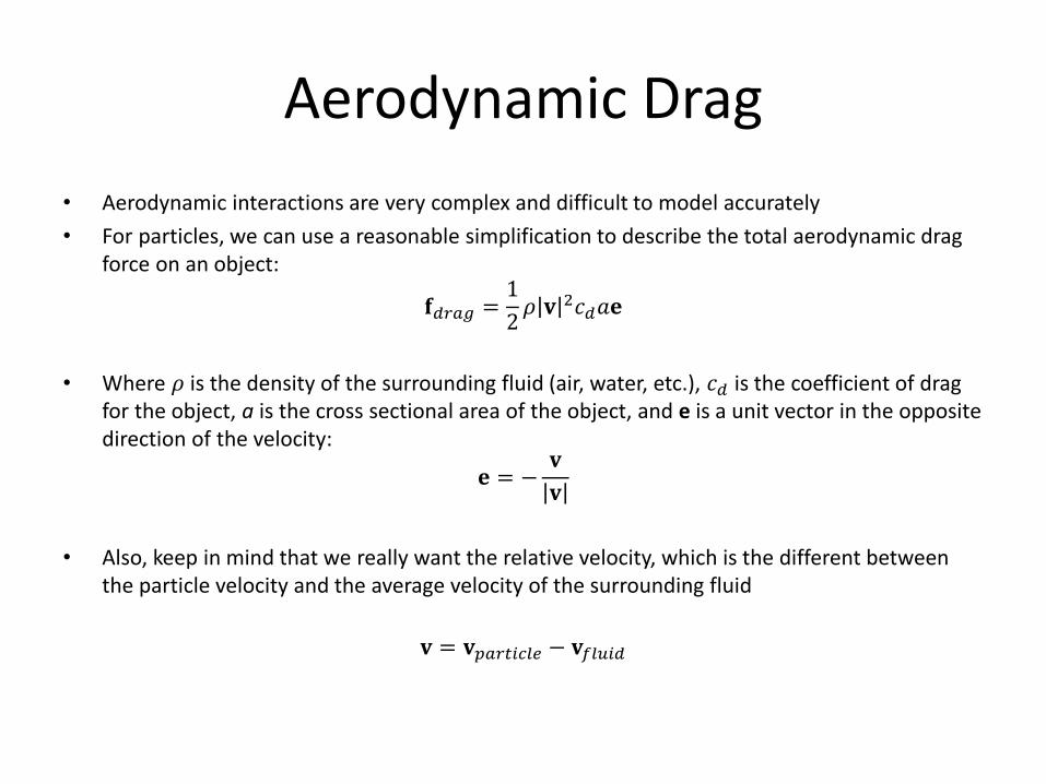
• Aerodynamic interactions are very complex and difficult to model accurately

• For particles, we can use a reasonable simplification to describe the total aerodynamic drag force on an object:

𝐟𝑑𝑟𝑎𝑔 =1

2𝜌 𝐯 2𝑐𝑑𝑎𝐞

• Where 𝜌 is the density of the surrounding fluid (air, water, etc.), 𝑐𝑑 is the coefficient of drag for the object, a is the cross sectional area of the object, and e is a unit vector in the opposite direction of the velocity:

𝐞 = −𝐯

𝐯

• Also, keep in mind that we really want the relative velocity, which is the different between the particle velocity and the average velocity of the surrounding fluid

𝐯 = 𝐯𝑝𝑎𝑟𝑡𝑖𝑐𝑙𝑒 − 𝐯𝑓𝑙𝑢𝑖𝑑

Fluid Density: 𝜌

𝐟𝑑𝑟𝑎𝑔 =1

2𝜌 𝐯 2𝑐𝑑𝑎𝐞

• The fluid density 𝜌 of air at 15o C and a pressure of 101.325 kPa (14.696 psi) is 1.225 kg/m3 and is used as a common default value

• For aircraft simulations, one could use more advanced density models that vary with altitude, temperature, and humidity

• The fluid density 𝜌 of liquid water is 999.8 kg/m3 at 0o

C and 997.0 kg/m3 at 25o C at sea level

Drag Coefficient: 𝑐𝑑

𝐟𝑑𝑟𝑎𝑔 =1

2𝜌 𝐯 2𝑐𝑑𝑎𝐞

• The aerodynamic drag force uses a unit-less constant 𝑐𝑑 called the drag coefficient

• This number effectively quantifies the aerodynamic drag of the particular shape, and typically ranges from around 0.01 (very streamlined) to 1.5 (bluff body)

• A sphere has a 𝑐𝑑 around 0.47 and a cube has a 𝑐𝑑 around 1.05• The Tesla Model 3 has a 𝑐𝑑 of 0.23 and a Jeep Wrangler has a 𝑐𝑑 of 0.58• A person on a bicycle has a 𝑐𝑑 around 1.0 and a person running has a

𝑐𝑑 around 1.2• A Formula-1 race car actually has a 𝑐𝑑 near 1.4! This is because the

aerodynamics of the car body are designed to generate downforce to keep the car on the ground in tight turns. This downforce has to increase drag due to conservation of momentum

Cross Sectional Area: 𝑎

𝐟𝑑𝑟𝑎𝑔 =1

2𝜌 𝐯 2𝑐𝑑𝑎𝐞

• In the aerodynamic drag equation above, a refers to the cross sectional area of the object moving through the surrounding fluid

• This means the area when viewed from the direction of motion

• For a spherical object of radius r, it would be 𝜋𝑟2

• For a car driving forward, this would be the area of the front of the car viewed with an orthographic projection

Aerodynamic Drag

𝐟𝑑𝑟𝑎𝑔 =1

2𝜌 𝐯 2𝑐𝑑𝑎𝐞

• Most of the values here are constants (𝜌, 𝑐𝑑, 𝑎), and eis just used to specify the direction the force acts

• Therefore, when we really boil this down, we see that the aerodynamic drag force is proportional to velocity squared

𝑓𝑑𝑟𝑎𝑔 ∝ 𝑣2

Springs

• We can use Hooke’s Law to model simple linear spring forces:

𝐟𝑠𝑝𝑟𝑖𝑛𝑔 = −𝑘𝑠𝐱

• Where 𝑘𝑠 is the spring constant describing the stiffness of the spring and x is a vector describing the displacement

• The spring force is therefore going to work against the displacement

• The direction of the force will be along the axis of the spring and will pull if the spring is extended and push if the spring is compressed

Springs

• In practice, it’s nice to define a spring as connecting two particles and having a rest length 𝑙0 where the spring force is 0

• This gives us:

𝑥 = 𝐫1 − 𝐫2 − 𝑙0

𝐞 =𝐫1−𝐫2

𝐫1−𝐫2

𝐱 = 𝑥𝐞

𝑙0

𝑙0𝑥

𝐫1 𝐫2

𝐫1 𝐫2

𝐱

Springs

• A spring applies equal and opposite forces to two particles, and therefore explicitly obeys Newton’s Third Law

• They should also obey the Laws of Conservation of Momentum and Conservation of Energy

• In practice however, how well they obey these laws is due to the numerical integration scheme used

• We will discuss this in more detail in the next lecture

Dampers

• We can apply damping forces between particles:

𝐟𝑑𝑎𝑚𝑝 = −𝑘𝑑𝑣𝑐𝑙𝑜𝑠𝑒𝐞

• 𝑘𝑑 is the damping constant, 𝑣𝑐𝑙𝑜𝑠𝑒 is the closing velocity, and 𝐞 is a unit vector that provides the direction (𝐞 works the same as with springs)

• Dampers will oppose any difference in velocity between particles• The damping forces are equal and opposite, so they should conserve

momentum, but they will remove energy from the system by design• In real dampers, kinetic energy of motion is converted into complex fluid

motion within the damper and then diffused into random molecular motion in the form of heat

• In other words, the kinetic energy of motion is effectively lost, but Conservation of Energy is still obeyed because the kinetic energy is converted into thermal energy

Closing Velocity

• To calculate the damping force, we need to calculate the closing velocity between two particles

• This is the rate that the two particles are approaching each other

𝑣𝑐𝑙𝑜𝑠𝑒 = 𝐯2 − 𝐯1 ∙ 𝐞

𝐫2𝐫1

𝐯2

𝐯1𝐞

Spring-Dampers

• It is common to combine a spring and a damper into a single entity called a spring-damper

• A spring-damper connects two particles and has a rest length 𝑙0, a spring constant 𝑘𝑠, and a damping constant 𝑘𝑑

Spring-Damper Example

class SpringDamper {public:

void ComputeForces();private:

Particle *P1,*P2;float SpringConstant;float DampingConstant;float RestLength;

};

Spring-Damper Example

SpringDamper::ComputeForces() {// Get kinematic particle propertiesconst vec3 &r1=P1->GetPosition(), &r2=P2->GetPosition();const vec3 &v1=P1->GetVelocity(), &v2=P2->GetVelocity();

// Compute kinematic properties based on both particlesfloat dist=distance(r1,r2); // Distance between particlesvec3 e=(r1-r2)/dist; // Unit vector for directionfloat x=dist-RestLength; // Displacementfloat v=dot((v2-v1),e); // Closing velocity

// Compute spring-damper forcevec3 force=(- SpringConstant*x - DampingConstant*v ) * e;

// Apply force to particlesP1->ApplyForce(force); // Apply force to P1P2->ApplyForce(-force); // Apply equal and opposite force to P2

}

Combining Forces

• All of the different forces we’ve examined can be combined by simply adding them together

• The total force on a particle is just the sum of all of the individual forces

• In each step of the simulation, we compute all of the forces in the entire system at the particular instant

• We then use those forces to integrate the accelerations to compute new velocities and positions at some finite time step later