next-generation nato reference mobility model using …€¦ · generation nato reference mobility...

2019 NDIA GROUND VEHICLE SYSTEMS ENGINEERING AND TECHNOLOGY SYMPOSIUM

MODELING & SIMULATION, TEST & VALIDATION TECHNICAL SESSION AUGUST 13-15, 2019 - NOVI, MICHIGAN

NEXT-GENERATION NATO REFERENCE MOBILITY MODEL USING ROAMS SIMULATION FOR DEMONSTRATION OF TECHNOLOGY -

VERIFICATION AND VALIDATION

Ole Balling, PhD1, Morten Rydahl-Haastrup, PhD1, Louise Bendtsen1, Frederik Homaa1

Christopher S. Lim2, Aaron Gaut2, Abhinandan Jain, PhD2

1Department of Engineering, Section of Mechanical and Materials Engineering,

Aarhus University, Aarhus, Denmark

2Jet Propulsion Laboratory/California Institute of Technology, Pasadena, CA

ABSTRACT

The work presented in this contribution demonstrates the results of the verification and validation efforts of simulation versus test of the mobility of a light tactical vehicle, the Fuel Efficiency Demonstrator, FED-Alpha. The simulations are the contribution to the Cooperate Demonstration of Technology (CDT) of Next Generation NATO Reference Mobility Model as performed by the Aarhus University (AU) team using Jet Propulsion Laboratory’s (JPL) ROver Analysis, Modeling and Analysis Software ROAMS. The work demonstrates hard surface automotive tests as well as soft soil tire-terrain terramechanics tests such as drawbar pull on fine and coarse grained soils and a variable sand slope test on coarse grained soil. Furthermore, a traverse of mixed terrain types and the results of a developed off-road driver model are shown as a demonstrator of Next-Generation NATO Reference Mobility Model simulation capability.

Citation: O. Balling, M. Rydahl-Haastrup, L. Bendtsen, F. Homaa, C. Lim, A. Gaut, A. Jain, “Next-Generation NATO Reference Mobility Model Using ROAMS Simulation for Demonstration of Technology – Verification and Validation”, In Proceedings of the Ground Vehicle Systems Engineering and Technology Symposium (GVSETS), NDIA, Novi, MI, Aug. 13-15, 2019.

1. INTRODUCTION

This paper has two parts. The first part concerns the vehicle simulation in ROAMS. The methods and theories for the involved simulation aspects are explained here. The second part concerns the execution in simulation and results of the individual

vehicle tests as required for the CDT. This includes details on the implementation using the vehicle and soil data from Keweenaw Research Center (KRC) and insights into how the virtual vehicle tests were conducted in ROAMS.

Proceedings of the 2019 Ground Vehicle Systems Engineering and Technology Symposium (GVSETS)

“Next-Generation NATO Reference Mobility Model Using ROAMS Simulation for Demonstration of Technology – Verification and Validation”, O. Balling et al.

of 18

2. ROAMS IMPLEMENTATION The ROAMS software is made available to

Aarhus University through a research-use license agreement between Aarhus University and Jet Propulsion Laboratory at California Institute of Technology. ROAMS is developed at JPL’s Dynamics Algorithms for Real-Time Simulation Laboratory, DARTS Lab. The DARTS Lab provides several multi-mission space system simulation tools for the closed-loop development and testing of flight algorithms and software. This toolkit can be used in workstation environments as well as in real-time, hardware-in-the-loop simulations for the testing and verification of flight software and hardware. ROAMS (Rover Analysis, Modeling and Simulation) is a physics based simulation tool for the analysis, design, development, test and operation of rovers for planetary surface exploration missions. ROAMS provides a modular rover simulation framework to facilitate its use by planetary exploration missions for system engineering studies, technology development, and mission operation teams. ROAMS is currently being developed and used by NASA's Mars Program as a virtual testing ground for various rover subsystems and components. ROAMS is a rover specific extension of the multi-mission DARTS and DSHELL spacecraft simulation toolkit, which is capable of modeling vehicle dynamics, engineering sensors and actuators, environments and is in use by several missions such as Cassini, Space Interferometry Mission, Deep Space 1, Mars Science Laboratory etc.

Figure 1: The FED-Alpha in ROAMS

ROAMS provides a library of high fidelity

models for the surface rover. Its modular architecture permits the user to configure the modular structure simulation tailored to specific needs and fidelity. For instance different rover vehicles, environments, navigation modes etc. can be defined for creating the simulation of the vehicle performance. The simulation framework and the graphical representation of the FED-Alpha vehicle is illustrated in Figure 1. ROAMS can also be used for real-time simulations using the real-time features of the underlying Darts/Dshell simulation toolkit [1].

2.1. Terrain data

To enable the use of the ROAMS simulation framework for the prediction of mobility of the FED-Alpha vehicle, the KRC terrain information provided in the GeoTIFF format was used. The GeoTIFF metadata format allows geo-referencing to be embedded within the tiff file. The metadata can contain additional information such as elevation, soil type and specific soil properties. The SIMSCAPE toolkit [2] from JPL was used to get the KRC terrain data into an x-y grid of elevation or mesh suitable for vehicle simulation. SIMSCAPE provides a common infrastructure to import terrain data from multiple sources. The tire model in ROAMS is able to use the information and compute the tire forces using the elevation and soil properties of the wheel location. The spatial resolution of a GeoTIFF depends on the highest resolution of the data sources available. In the case of the KRC terrain, the elevation data provided the highest resolution such that a pixel represents an area of approximate 7 by 7 centimeters. This elevation data is combined with the actual measured surface and soil parameters such as coefficient of friction and Bekker-Wong data where applicable.



of 18

2.2. The FED-Alpha in ROAMS The multibody dynamics formulation behind the

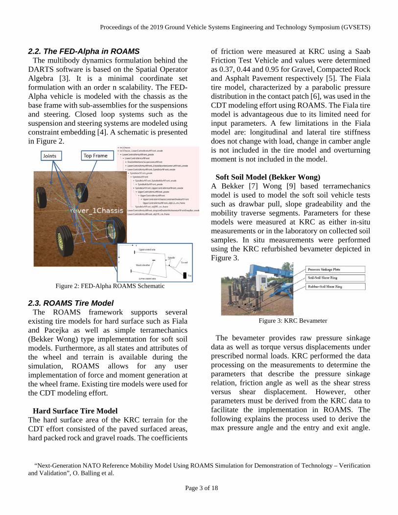
DARTS software is based on the Spatial Operator Algebra [3]. It is a minimal coordinate set formulation with an order n scalability. The FED-Alpha vehicle is modeled with the chassis as the base frame with sub-assemblies for the suspensions and steering. Closed loop systems such as the suspension and steering systems are modeled using constraint embedding [4]. A schematic is presented in Figure 2.

Figure 2: FED-Alpha ROAMS Schematic

2.3. ROAMS Tire Model

The ROAMS framework supports several existing tire models for hard surface such as Fiala and Pacejka as well as simple terramechanics (Bekker Wong) type implementation for soft soil models. Furthermore, as all states and attributes of the wheel and terrain is available during the simulation, ROAMS allows for any user implementation of force and moment generation at the wheel frame. Existing tire models were used for the CDT modeling effort.

Hard Surface Tire Model

The hard surface area of the KRC terrain for the CDT effort consisted of the paved surfaced areas, hard packed rock and gravel roads. The coefficients

of friction were measured at KRC using a Saab Friction Test Vehicle and values were determined as 0.37, 0.44 and 0.95 for Gravel, Compacted Rock and Asphalt Pavement respectively [5]. The Fiala tire model, characterized by a parabolic pressure distribution in the contact patch [6], was used in the CDT modeling effort using ROAMS. The Fiala tire model is advantageous due to its limited need for input parameters. A few limitations in the Fiala model are: longitudinal and lateral tire stiffness does not change with load, change in camber angle is not included in the tire model and overturning moment is not included in the model.

Soft Soil Model (Bekker Wong)

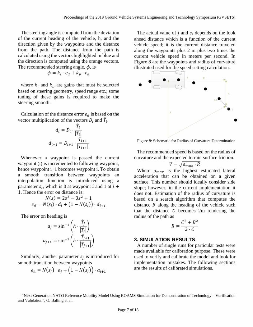
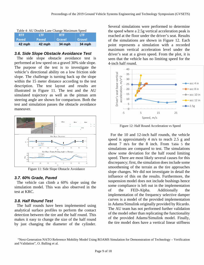
A Bekker [7] Wong [9] based terramechanics model is used to model the soft soil vehicle tests such as drawbar pull, slope gradeability and the mobility traverse segments. Parameters for these models were measured at KRC as either in-situ measurements or in the laboratory on collected soil samples. In situ measurements were performed using the KRC refurbished bevameter depicted in Figure 3.

Figure 3: KRC Bevameter

The bevameter provides raw pressure sinkage

data as well as torque versus displacements under prescribed normal loads. KRC performed the data processing on the measurements to determine the parameters that describe the pressure sinkage relation, friction angle as well as the shear stress versus shear displacement. However, other parameters must be derived from the KRC data to facilitate the implementation in ROAMS. The following explains the process used to derive the max pressure angle and the entry and exit angle.



of 18

These depend on the sinkage and the restitution of the soil after the wheel has passed.

The pressure sinkage relation is the cornerstone in the Bekker soft soil model [7]. It is defined as:

𝑝𝑝 = �𝑘𝑘𝑐𝑐𝑏𝑏

+ 𝑘𝑘𝑝𝑝ℎ𝑖𝑖� ⋅ 𝑧𝑧𝑛𝑛 or

𝑝𝑝 = 𝑘𝑘𝑒𝑒𝑒𝑒 ⋅ 𝑧𝑧𝑛𝑛 (1) The parameters used in the drawbar pull

simulations are listed in Table 1. The parameters are derived by KRC based on in situ soft soil test using the KRC bevameter [8]. 𝑘𝑘𝑐𝑐 and 𝑘𝑘𝜙𝜙are the cohesive and frictional moduli of deformation and b is the smaller of the loading area. If the value of 𝑘𝑘𝜙𝜙 is negative, 𝑘𝑘𝑒𝑒𝑒𝑒 is used and 𝑘𝑘𝑐𝑐 is set to zero. The value of 𝑛𝑛 is also adjusted in this case.

The shear modulus K and cohesion c does depend on the tread pattern on the tire, because the shear force transfer is different in soil-soil contact and rubber-soil contact. Aberdeen Test Center has measured the area of rubber contact with the ground on hard surface in [10]. The net contact area and rubber contact area are depicted versus tire inflation pressure and tire normal load. From this table it was calculated that 58% of the contact patch is rubber-soil. The remaining is soil-soil contact. This ratio was used in calculating the shear modulus K and the cohesion c in Table 1.

Table 1. Measured soil parameters for the Bekker model. Soil type 𝒏𝒏 𝒌𝒌𝒆𝒆𝒆𝒆 𝑲𝑲 𝒄𝒄 𝝓𝝓

𝑁𝑁𝑚𝑚𝑛𝑛+2 mm Pa deg

FGS Dry (1) 1.55 9.96E+04 13.6 441 32.3

FGS Dry (2) 1.92 5.37E+05 11.1 612.5 31.9

CGS Dry (1) 0.55 1686 13 840.2 28.1

CGS Dry (2) 0.74 2765 15.7 597.9 28.9

CGS Dry (3) 0.87 3367 15 488.4 29

FGS Wet (1) 4.39 8.24E+06 15.4 1552.8 32.3

FGS Wet (2) 3.68 5.20E+05 17.9 1996.8 30.6

In the implementation of the Bekker model in ROAMS, values for max pressure angle and exit angle are needed. These values are estimated from the calculations presented below. First step is to estimate the nominal sinkage given a rigid wheel on soft soil. The pressure under a tire can be estimated using the pressure sinkage relation, equation (4.1) in [9], which is reprinted below.

𝑝𝑝 = 𝑘𝑘𝑒𝑒𝑒𝑒 ⋅ 𝑧𝑧𝑛𝑛 (1) Assuming that the pressure calculated is the

average pressure, then it must equal the load on the tire divided by the area. However, the area increases as the tire is loaded.

Figure 4: Sketch for the calculation of sinkage.

𝑝𝑝 =𝑊𝑊𝐴𝐴

=𝑊𝑊

2 ⋅ 𝑙𝑙 ⋅ 𝑏𝑏=

𝑊𝑊2 ⋅ �2 ⋅ 𝑟𝑟𝑛𝑛 ⋅ 𝑧𝑧 − 𝑧𝑧2 ⋅ 𝑏𝑏

=1370𝑘𝑘𝑘𝑘 ⋅ 9.81 𝑁𝑁

𝑘𝑘𝑘𝑘2 ⋅ √2 ⋅ 0.4987 ⋅ 𝑧𝑧 − 𝑧𝑧2 ⋅ 0.335

(2)

Setting this equation equal to equation (1), it is

possible to calculate the sinkage, z.



of 18

Figure 5: Sketch for the calculation of exit angle and max

pressure angle. The approach of repetitive loading [9] is used to

calculate the elastic part of the unloading of the soil. The surface pressure after the wheel has passed is zero. Hence, equation 4.23 in [9] is set to zero.

𝑝𝑝 = 0 = 𝑘𝑘𝑒𝑒𝑒𝑒 ⋅ 𝑧𝑧𝑛𝑛 − 𝑘𝑘𝑢𝑢 ⋅ (𝑧𝑧 − 𝑧𝑧𝑒𝑒) 𝑘𝑘𝑢𝑢 = 𝑘𝑘0 + 𝐴𝐴𝑢𝑢 ⋅ 𝑧𝑧

𝑧𝑧𝑒𝑒 = 𝑧𝑧 −𝑘𝑘𝑒𝑒𝑒𝑒 ⋅ 𝑧𝑧𝑛𝑛

𝑘𝑘0 + 𝐴𝐴𝑢𝑢 ⋅ 𝑧𝑧

The numbers 𝑘𝑘𝑢𝑢 and 𝐴𝐴𝑢𝑢 are obtained from

measurements and is provided for each of the soil type.

For some of the Design of Experiment (DoE) runs the AU team was asked to perform for the uncertainty quantification, 𝑧𝑧𝑒𝑒 become negative meaning that the compression curve is steeper than the release curve. This does not make sense from a physical point of view, hence for those cases 𝑧𝑧𝑒𝑒 = 𝑧𝑧.

Some of the soils in the DoE-runs were specified quite firm with a sinkage of only a few millimeters. In those cases, the tire deformation is significant. The nominal radius of the tire is 𝑟𝑟𝑛𝑛 = 0.498𝑚𝑚 and the rolling radius is 𝑟𝑟𝑟𝑟 = 0.453. It was chosen to add the difference in radii to the sinkage when calculating the maximum pressure angle θ𝑚𝑚 and the exit angle 𝜃𝜃𝑒𝑒. The tire deformation was

accounted for by doing so. The exit angle as illustrated in Figure 5 is:

𝜃𝜃𝑒𝑒 = − cos−1 �𝑟𝑟𝑛𝑛 − 𝑧𝑧𝑒𝑒 − (𝑟𝑟𝑛𝑛 − 𝑟𝑟𝑟𝑟)

𝑟𝑟𝑛𝑛�

For calculation of the maximum pressure angle, it

is assumed that the pressure distribution underneath the tire is symmetric in the region between the entry and exit angle. Lack of detailed information of the variation of the location of the maximum pressure angle for the soils assigned for simulation is the reason for this assumption.

𝜃𝜃1 = cos−1 �𝑟𝑟𝑛𝑛 − 𝑧𝑧 − (𝑟𝑟𝑛𝑛 − 𝑟𝑟𝑟𝑟)

𝑟𝑟𝑛𝑛�

𝜃𝜃𝑚𝑚 = (𝜃𝜃1 + 𝜃𝜃𝑒𝑒) ⋅ 0.5

Table 2: Soil parameters used in the drawbar pull simulations for the Bekker model continued.

Soil type 𝒛𝒛 𝒛𝒛𝒆𝒆 𝜽𝜽𝒎𝒎 𝜽𝜽𝒆𝒆

mm mm deg deg

FGS Dry (1) 15.9 1 1.88 -25.11

FGS Dry (2) 14.9 1.1 1.75 -25.13

CGS Dry (1) 14.7 1.1 1.73 -25.12

CGS Dry (2) 19.2 0.9 2.29 -25.07

CGS Dry (3) 24.2 0.7 2.88 -25.03

FGS Wet (1) 71.6 0.8 7.56 -25.05

FGS Wet (2) 88.8 0.6 9.08 -24.99

2.4. Drivetrain Model

The drivetrain consists of front, rear and center differential, gearbox, transfer case, torque converter and engine. The drivetrain model is based on a semi kinematic approach where throttle position, angular speed and acceleration of the wheels are given as inputs and the torque at each wheel is the output. The wheel speeds are entering through the differentials, transfer case and gearbox to the engine while being multiplied by the appropriate gear ratio at each junction with a gearing. The torque travels the other way through the drivetrain, and is multiplied by efficiencies as



of 18

well as gear ratios along the way as illustrated in Figure 6.

Figure 6: Drivetrain Schematic and Engine Torque Curve

Differentials The speed and acceleration of the shaft towards

the gearbox (low speed side) is the average speed of the wheels times the gear ratio of the differentials. Logarithmic filtering is used at this stage on the angular velocity and acceleration to avoid transfer of small changes in wheel torque from the tire model to the engine. This has proven to be necessary, and the filtering accounts for some flexibility and damping in the drivetrain. Some of the CDT tests are conducted with open differentials, meaning the torque is equally distributed to all wheels. If a wheel loses traction, it will accelerate. With locked differentials, the wheels must rotate with the same speed. This is implemented by applying a PID-controller that adjusts the torque applied to each wheel to keep equal rotational velocity.

Gearbox The Fed-Alpha has a six gear automatic gearbox

with a high and low range for a total of 12 different combinations of gear ratio. All the gear ratios and efficiencies were supplied with the FED-Alpha vehicle data set [11]. The AU team have implemented both automatic and manual (fixed) gear selection.

Engine The engine model is based on a lookup table

smoothened by use of an Akima spline [13]. For a given engine rpm the corresponding torque is

computed using the performance curve stored in the lookup table. The engine torque map for full throttle is presented in Figure 6. The engine inertia is accounted for when determining available torque.

2.5. Springs and Dampers

The suspension springs of the vehicle are nonlinear. Their stiffness is also implemented using Akima splines.

The dampers are frequency dependent, so-called FSD (Frequency Selective Dampers). Two sets of measured damping have been made available: low and high frequency respectively. The damping curves are also implemented as Akima splines. The input to the function returning the damping values is speed and the output is force. The splines are almost identical when the damper is in jounce, i.e. the speed is negative. A first order filter can remove high frequency content from the speed signal; hence, the filtered velocity can be used for determining if the high or low frequency spline should be used.

2.6. Driver Model

The driver model has two parts: an algorithm for computing the steering angle and another for predicting the highest safe speed at a given location taking into account upcoming corners and current velocity. The driver model is designed to follow waypoints recorded with a GPS with close to uniform spacing. The AU team used waypoints for the CDT that are located at about 1m spacing. The driver model and its use of waypoints are illustrated in Figure 7.

Figure 7: Schematic of AU Driver Model's use of

Waypoints



of 18

The steering angle is computed from the deviation of the current heading of the vehicle, h, and the direction given by the waypoints and the distance from the path. The distance from the path is calculated using the vectors highlighted in blue and the direction is computed using the orange vectors. The recommended steering angle, 𝜙𝜙, is

𝜙𝜙 = 𝑘𝑘𝑖𝑖 ⋅ 𝑒𝑒𝑑𝑑 + 𝑘𝑘𝑝𝑝 ⋅ 𝑒𝑒ℎ where 𝑘𝑘𝑖𝑖 and 𝑘𝑘𝑝𝑝 are gains that must be selected

based on steering geometry, speed range etc.; some tuning of these gains is required to make the steering smooth.

Calculation of the distance error 𝑒𝑒𝑑𝑑 is based on the

vector multiplication of the vectors 𝐷𝐷𝑖𝑖 and 𝑇𝑇�𝑖𝑖.

𝑑𝑑𝑖𝑖 = 𝐷𝐷𝑖𝑖 ⋅𝑇𝑇�𝑖𝑖

|𝑇𝑇𝑖𝑖|

𝑑𝑑𝑖𝑖+1 = 𝐷𝐷𝑖𝑖+1 ⋅𝑇𝑇�𝑖𝑖+1

|𝑇𝑇𝑖𝑖+1|

Whenever a waypoint is passed the current

waypoint (i) is incremented to following waypoint, hence waypoint i+1 becomes waypoint i. To obtain a smooth transition between waypoints an interpolation function is introduced using a parameter 𝑠𝑠𝑖𝑖, which is 0 at waypoint 𝑖𝑖 and 1 at 𝑖𝑖 +1. Hence the error on distance is:

𝑁𝑁(𝑠𝑠) = 2𝑠𝑠3 − 3𝑠𝑠2 + 1 𝑒𝑒𝑑𝑑 = 𝑁𝑁(𝑠𝑠𝑖𝑖) ⋅ 𝑑𝑑𝑖𝑖 + �1 − 𝑁𝑁(𝑠𝑠𝑖𝑖)� ⋅ 𝑑𝑑𝑖𝑖+1

The error on heading is

𝑎𝑎𝑗𝑗 = sin−1 �ℎ ⋅𝑇𝑇�𝑗𝑗�𝑇𝑇𝑗𝑗�

�

𝑎𝑎𝑗𝑗+1 = sin−1 �ℎ ⋅𝑇𝑇�𝑗𝑗+1�𝑇𝑇𝑗𝑗+1�

�

Similarly, another parameter 𝑠𝑠𝑗𝑗 is introduced for

smooth transition between waypoints 𝑒𝑒ℎ = 𝑁𝑁�𝑠𝑠𝑗𝑗� ⋅ 𝑎𝑎𝑗𝑗 + �1 − 𝑁𝑁�𝑠𝑠𝑗𝑗�� ⋅ 𝑎𝑎𝑗𝑗+1

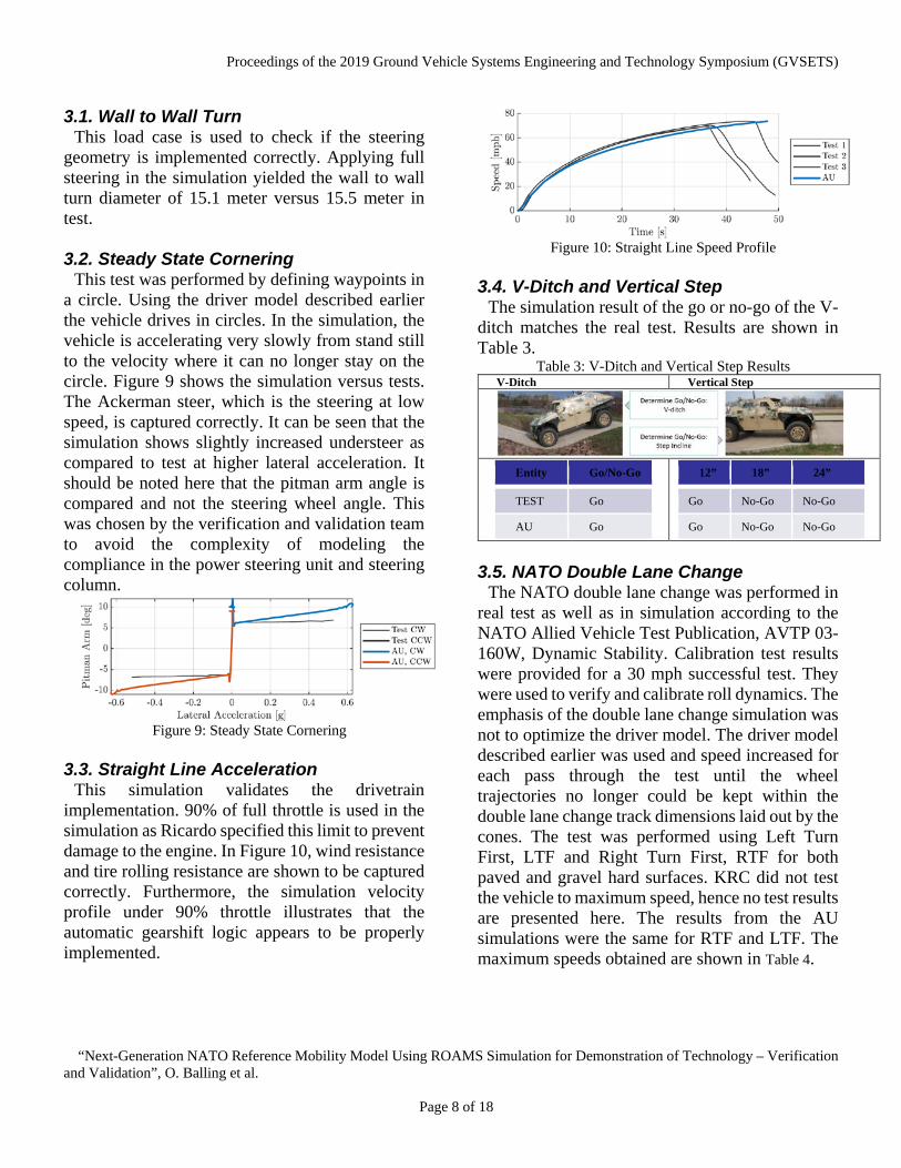
The actual value of 𝑗𝑗 and 𝑠𝑠𝑗𝑗 depends on the look ahead distance which is a function of the current vehicle speed; it is the current distance traveled along the waypoints plus 2 m plus two times the current vehicle speed in meters per second. In Figure 8 are the waypoints and radius of curvature illustrated used for the speed setting calculation.

Figure 8: Schematic for Radius of Curvature Determination The recommended speed is based on the radius of

curvature and the expected terrain surface friction. 𝑉𝑉 = �𝑎𝑎𝑚𝑚𝑚𝑚𝑚𝑚 ⋅ 𝑅𝑅

Where 𝑎𝑎𝑚𝑚𝑚𝑚𝑚𝑚 is the highest estimated lateral acceleration that can be obtained on a given surface. This number should ideally consider side slope; however, in the current implementation it does not. Estimation of the radius of curvature is based on a search algorithm that computes the distance 𝐵𝐵 along the heading of the vehicle such that the distance 𝐶𝐶 becomes 2m rendering the radius of the path as

𝑅𝑅 =𝐶𝐶2 + 𝐵𝐵2

2 ⋅ 𝐶𝐶

3. SIMULATION RESULTS

A number of single runs for particular tests were made available for calibration purpose. These were used to verify and calibrate the model and look for implementation mistakes. The following sections are the results of calibrated simulations.



of 18

3.1. Wall to Wall Turn This load case is used to check if the steering

geometry is implemented correctly. Applying full steering in the simulation yielded the wall to wall turn diameter of 15.1 meter versus 15.5 meter in test.

3.2. Steady State Cornering

This test was performed by defining waypoints in a circle. Using the driver model described earlier the vehicle drives in circles. In the simulation, the vehicle is accelerating very slowly from stand still to the velocity where it can no longer stay on the circle. Figure 9 shows the simulation versus tests. The Ackerman steer, which is the steering at low speed, is captured correctly. It can be seen that the simulation shows slightly increased understeer as compared to test at higher lateral acceleration. It should be noted here that the pitman arm angle is compared and not the steering wheel angle. This was chosen by the verification and validation team to avoid the complexity of modeling the compliance in the power steering unit and steering column.

Figure 9: Steady State Cornering

3.3. Straight Line Acceleration

This simulation validates the drivetrain implementation. 90% of full throttle is used in the simulation as Ricardo specified this limit to prevent damage to the engine. In Figure 10, wind resistance and tire rolling resistance are shown to be captured correctly. Furthermore, the simulation velocity profile under 90% throttle illustrates that the automatic gearshift logic appears to be properly implemented.

Figure 10: Straight Line Speed Profile

3.4. V-Ditch and Vertical Step

The simulation result of the go or no-go of the V-ditch matches the real test. Results are shown in Table 3.

Table 3: V-Ditch and Vertical Step Results V-Ditch Vertical Step

Entity Go/No-Go

TEST Go

AU Go

12” 18” 24”

Go No-Go No-Go

Go No-Go No-Go

3.5. NATO Double Lane Change

The NATO double lane change was performed in real test as well as in simulation according to the NATO Allied Vehicle Test Publication, AVTP 03-160W, Dynamic Stability. Calibration test results were provided for a 30 mph successful test. They were used to verify and calibrate roll dynamics. The emphasis of the double lane change simulation was not to optimize the driver model. The driver model described earlier was used and speed increased for each pass through the test until the wheel trajectories no longer could be kept within the double lane change track dimensions laid out by the cones. The test was performed using Left Turn First, LTF and Right Turn First, RTF for both paved and gravel hard surfaces. KRC did not test the vehicle to maximum speed, hence no test results are presented here. The results from the AU simulations were the same for RTF and LTF. The maximum speeds obtained are shown in Table 4.



of 18

Table 4: AU Double Lane Change Maximum Speed

RTF Paved

LTF Paved

RTF Gravel

LTF Gravel

42 mph 42 mph 34 mph 34 mph

3.6. Side Slope Obstacle Avoidance Test The side slope obstacle avoidance test is

performed at low speed on a gravel 30% side slope. The purpose of the test is to investigate the vehicle’s directional ability on a low friction side slope. The challenge is turning back up the slope within the 15 meter distance according to the test description. The test layout and results are illustrated in Figure 11. The test and the AU simulated trajectory as well as the pitman arm steering angle are shown for comparison. Both the test and simulation passes the obstacle avoidance maneuver.

Figure 11: Side Slope Obstacle Avoidance

3.7. 60% Grade, Paved

The vehicle can climb a 60% slope using the simulation model. This was also observed in the test at KRC.

3.8. Half Round Test

The half rounds have been implemented using analytical surface profiles to perform the contact detection between the tire and the half round. This makes it easy to change the size of the half round by just changing the diameter of the cylinder.

Several simulations were performed to determine the speed where a 2.5g vertical acceleration peak is reached at the floor under the driver’s seat. Results of the simulations are shown in Figure 12. Each point represents a simulation with a recorded maximum vertical acceleration level under the driver’s seat at a given speed. From the plot, it is seen that the vehicle has no limiting speed for the 4-inch half round.

Figure 12: Half Round Acceleration vs Speed

For the 10 and 12-inch half rounds, the vehicle

speed is approximately 4 m/s to reach 2.5 g and about 7 m/s for the 8 inch. From Table 5 the simulations are compared to test. The simulations show some deviation for the half round limiting speed. There are most likely several causes for this discrepancy; first, the simulation does include some smoothening of the terrain as the tire approaches slope changes. We did not investigate in detail the influence of this on the results. Furthermore, the suspension model does not include bushings hence some compliance is left out in the implementation of the FED-Alpha. Additionally the implementation of the frequency selective damper curves is a model of the provided implementation in Adams/Simulink originally provided by Ricardo. The AU team has not performed further validation of the model other than replicating the functionality of the provided Adams/Simulink model. Finally, the tire model does have a vertical linear stiffness

0

5

10

15

20

25

30

35

40

-5 5 15 25Dr

iver

's se

at b

ase

vert

ical

ac

cele

ratio

n, m

/s^2

Speed, m/s

acc 4 in

acc 8 in

acc 10 in

acc 12 in

2.5g



of 18

of the tire, but this is possibly too simplistic for the large deflection the real tire exhibits as it travels over the half round. The first effect should allow for faster speeds and the two last points should cause lower speeds.

Table 5: 2.5g Half Round Limiting Speed (m/s)

Entity 4” 8” 10” 12”

TEST No Limit 9.8 8 6.7

AU No Limit 7 4.5 4

3.9. RMS Symmetric: Absorbed Power

The symmetric Root Mean Square (RMS) courses have been designed for the CDT. The desired courses were designed as RMS 1.0, 1.5, 2.0, 3.0, 4.0 inch. The courses were scanned after construction to measure their “as built” values. These are listed in Table 6. The courses are referred to their desired RMS value in the following.

Table 6: Desired and "As Built" RMS courses

Course: 1.0” 1.5” 2.0” 3.0” 4.0”

As Built: 1.06” 1.54” 1.99” 2.77” 3.88”

A number of straight-line runs along the

individual RMS courses each at a different speed were completed. The absorbed power was computed using the vertical component of the seat base acceleration signal according to [12]. The resulting data is presented in Figure 13 with linear interpolation between the data points. The crossing of the 6 watt absorbed line yields the absorbed power. Improved approximation of the 6 watt absorbed speed of an RMS course can be obtained by performing additional speed runs around the 6 watt crossing. The 6 watt speed are compared to test in mph in Table 7. Some deviation from test is found and can be attributed to the same reasons listed in the half round section.

Table 7: AU and Test 6 Watt Absorbed Power Speed

(mph) for 5 Symmetric RMS Courses

Course: 1.0” 1.5” 2.0” 3.0” 4.0”

Test 15.0 13.7 10.7 10.7 10.1

AU 7.4 11.2 12.1 16.3 18.8

Figure 13: Symmetric RMS Absorbed Power versus Speed

3.10. Asymmetric RMS Absorbed Power The two asymmetric RMS tests are similar to the

symmetric one with the difference that the vehicle is straddling two separate RMS courses. For the first test, one side of the vehicle’s wheels is driven on the 1 inch course and the other side on the 1.5 inch. For the second test, one side of wheels is driven on the 1.5 inch and the other side on the 2 inch course. The absorbed power versus speed plots are presented in Figure 14.

Figure 14: Asymmetric RMS Absorbed Power versus Speed The comparison to test is presented in Table 8 with speed in mph.

Table 8: AU and Test 6 Watt Absorbed Power Speed (mph) for 2 Asymmetric RMS Courses



of 18

Asymmetric RMS Course: 1.0”-1.5” 1.5”-2”

Test 14.4 13.2

AU 22.0 17.0

3.11. Soft Soil Tests Drawbar Pull

Drawbar pull is the measure of a vehicle’s available force for pulling a load on flat terrain on either paved surface or soft soil. Drawbar pull can also be thought of as the vehicle’s tractive effort minus the motion resistance. The tractive effort is the force available from the drivetrain before deforming the soil and tire. Drawbar pull is often depicted as drawbar force normalized with vehicle weight against wheel slip. This plot is called drawbar coefficient versus slip and can be thought of as the vehicle’s ability to utilize its weight to tow a load on a given surface or soil. The total average slip s for the vehicle is calculated by:

𝑠𝑠 =𝜔𝜔𝑤𝑤 ⋅ 𝑟𝑟𝑟𝑟 − 𝑣𝑣𝜔𝜔𝑤𝑤 ⋅ 𝑟𝑟𝑟𝑟

⋅ 100

where 𝑣𝑣 is the vehicle speed, 𝜔𝜔𝑤𝑤 is the average

wheel speed and 𝑟𝑟𝑟𝑟 the rolling radius. Using this definition the slip is zero when there is no drawbar force and no rolling resistance depending on how the rolling radius is measured. The Technical Operating Procedure, TOP 2-2-604, calls for the rolling radius being calculated using the distance traveled for one revolution of the tire towed over paved surface. For the FED-Alpha this radius is approximately 0.45 meter. The vehicle is immobilized at 100% slip when the drawbar force is large enough to stop the vehicle.

It is preferable to have the test in steady state condition due to the complexity of the soil-tire interaction under dynamic conditions. A challenge in real testing is to keep the vehicle at constant slip for a period long enough to obtain steady state conditions due to variations in soil conditions, wheel rpm and vehicle speeds. Furthermore, the

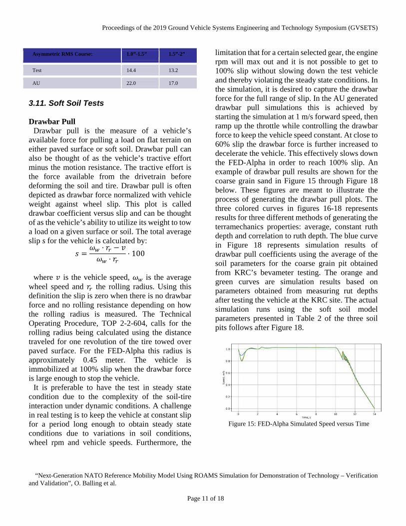
limitation that for a certain selected gear, the engine rpm will max out and it is not possible to get to 100% slip without slowing down the test vehicle and thereby violating the steady state conditions. In the simulation, it is desired to capture the drawbar force for the full range of slip. In the AU generated drawbar pull simulations this is achieved by starting the simulation at 1 m/s forward speed, then ramp up the throttle while controlling the drawbar force to keep the vehicle speed constant. At close to 60% slip the drawbar force is further increased to decelerate the vehicle. This effectively slows down the FED-Alpha in order to reach 100% slip. An example of drawbar pull results are shown for the coarse grain sand in Figure 15 through Figure 18 below. These figures are meant to illustrate the process of generating the drawbar pull plots. The three colored curves in figures 16-18 represents results for three different methods of generating the terramechanics properties: average, constant ruth depth and correlation to ruth depth. The blue curve in Figure 18 represents simulation results of drawbar pull coefficients using the average of the soil parameters for the coarse grain pit obtained from KRC’s bevameter testing. The orange and green curves are simulation results based on parameters obtained from measuring rut depths after testing the vehicle at the KRC site. The actual simulation runs using the soft soil model parameters presented in Table 2 of the three soil pits follows after Figure 18.

Figure 15: FED-Alpha Simulated Speed versus Time



of 18

Figure 16: FED-Alpha Simulated Throttle versus Time

Figure 17: FED-Alpha Drawbar Force versus Time

Figure 18: FED-Alpha Simulated Drawbar Pull Coefficient

(%) versus Slip for Coarse Grain Dry Soil In the following figures are the three drawbar pull

coefficient versus slip simulation results presented of the three KRC drawbar pull soil pits. The x-markers in the figures represents the first set of drawbar pull test data released from KRC with inertia correction. The individual color of the marker identifies separate test runs in the same pit. The full curves in the figures represent simulation results produced by the AU ROAMS model. The legend in the plots matches the naming of the soil properties presented in Table 1. It was chosen to make individual simulations with all Bekker parameters given for each individual soil pit to see the variation in the simulation results to the

different pit locations where the measurements were taken by KRC. In Figure 19 is the Fine Grain Sand Dry results presented. It is seen that the FGS_Dry2 parameters represent the test data well.

Figure 19: Drawbar Pull Coefficient, Fine Grain Sand –

Dry, X = Test The Fine Grain Sand Wet simulation and test

results are compared in Figure 20. Larger discrepancy was experienced in the Fine Grain Sand Wet. It is believed that the large flow of soil in this pit is posing a challenge for the simple terramechanics model. It should be noted that the ROAMS implementation for the CDT did not take multipass effects into account. The rear wheels sees undisturbed soil. This can be included in the ROAMS soft soil model by adding memory to the terrain about previous compaction history.

Figure 20: Drawbar Pull Coefficient, Fine Grain – Wet, X

= Test

0 20 40 60 80 100

Slip, %

0

0.1

0.2

0.3

0.4

0.5

0.6

Dra

wba

r coe

ffici

ent

FGS_Dry1

FGS_Dry2

0 20 40 60 80 100

Slip, %

0

0.1

0.2

0.3

0.4

0.5

0.6

Dra

wba

r coe

ffici

ent

FGS_Wet1

FGS_Wet2

FGS_Wet3



of 18

In Figure 21 is the Coarse Grain Sand drawbar pull simulation and test results presented. The coarse grain sand proved difficult to predict drawbar pull coefficient with the Bekker Wong based model and the bevameter data obtained in the field at KRC. This soil also exhibited large rut depth.

Figure 21: Drawbar Pull Coefficient, Coarse Grain – Dry,

X = Test The rut depths measured at KRC from the three

drawbar pull pits are presented in Table 9.

Table 9: Rut Depth Measured at KRC (cm)

The general conclusion from the drawbar pull

tests is that firm soil such as the Fine Grain – Dry drawbar pull performance was possible to capture with the Bekker Wong based model implemented in ROAMS. There were significant challenges in predicted reasonable drawbar pull performance on soils where large rut depths were measured. This leads to conclude that further investigations are needed to find the reason for the shortcomings of the implementation of the soft soil model in

ROAMS. There can be several reasons for that. The approximation of the maxium pressure location on the tire circumference being in the middle between entry and exit is a place of improvement. Moving this location closer to the soil entry point would increase the motion resistance and thereby lowering the drawbar pull results. However, with the data presented for this effort, the team did not have evidence to approximate this location different. Other places to look could be for the soil soil shear in the large rut depth soils. Possibly, the pressure in the tread pattern is not at a level supporting much shear due to soil flow out of the tread. At a given shear displacement it was found that the combined shear force generation from the soil soil and soil rubber engagement was dominated by the latter despite the higher friction angle for soil soil. The reason for this is the significant lower shear modulus for soil rubber.

Variable Grade Sand Slope The slope indicated by the orange elevation graph

in Figure 22 is the terrain used in the AU simulation of the vehicle performance on the sand slope. The blue curve is the vehicle center of gravity and the orange is the ground elevation as a function of distance traveled. The sand slope is composed of discrete steps in slope increments of 5% each.

Figure 22: Sand Slope, Variable Grade in Increments of

5% up through 60% Slope The simulated sand slope begins at level ground

and continues through 60% slope. The vehicle became immobilized at 40% slope as illustrated in the bottom plot of Figure 23 below.

0 20 40 60 80 100

Slip, %

0

0.1

0.2

0.3

0.4

0.5

0.6

Dra

wba

r coe

ffici

ent

CGS_Dry1

CGS_Dry2

CGS_Dry3

CGS_Dry4



of 18

Figure 23: Vehicle Velocities in the Vehicle Forward,

Lateral and Vertical Directions and Slope versus Time The vehicle accelerates while on the low grade

part of the sand slope. At about 15% incline the vehicle slows down. Engine torque and speed in rad/s are shown in the figure below along with the gear shifting.

Figure 24: Engine Torque (Nm), Speed (rad/s) and Gear The KRC variable grade was made of increments

of 15 degree. The FED-Alpha became immobilized with the front wheels at the 20% slope and the rear at the 15% slope. It was judged by KRC that the single number for gradeability should be 18.5%. A difference between the AU simulation and the KRC test is that the speed for the simulation was significantly larger than the at the test. This gives the vehicle additional linear momentum that can propel the vehicle higher up the slope. Another clear cause of the better performance of the simulation is related to the increased drawbar pull coefficient for the coarse grain sand. The soil type

of the sand slope was very similar to the coarse grain sand pit. Therefore the over prediction of the drawbar pull will cause the performance on the sand slope to over predict as well. It is expected that the maximum slope is not simply when the drawbar pull force measured at flat terrain is equal the vehicle weight times the sine of the slope angle. The shear as well as bearing capacity of the soil is expected to degrade on slopes.

3.12. Uncertainty Quantification

The CDT called for a demonstration of Uncertainty Quantification in the predicted Go-NoGo and Speed-Made-Good. Early in the process it was decided that the team from RAMDO Solutions, would supply software developers with Design of Experiment (DOE) soil parameters and slope for the developers to determine Go-NoGo and Speed-Made-Good. The AU team was provided with 100 combinations of soft soil parameters and slope. Simulations were designed that started the vehicle on flat terrain at low speed and then smoothly transitioned into the demanded slope. Throttle was then slowly increased till the vehicle reached a maximum speed. For some slope and soil combinations the vehicle could not move on the slope rendering a 0 or negative speed for a NoGo result. If the vehicle slid backward, 0 speed was reported as well. Average wheel slip was monitored and reported as well as the maximum speed obtained on the slope. The result was sent to RAMDO Solutions who processed the results and generated deterministic and a surrogate model to render confidence maps as depicted in Table 10 for Go-NoGo areas.

Table 10: Uncertainty Quantification, Confidence Intervals

on Go-NoGo Areas, 8kph Cut Off Speed

KRC CDT Area Overview

Deterministic Go-NoGo

Map Legend



of 18

10% Confidence Level









From the table it is observed that at low

confidence levels most of the KRC test area is green indicating Go. As the confidence level is increased, significant areas become red indicating NoGo. At the 90% confidence levels mainly the hard surface and flat areas are Go.

Table 11: Uncertainty Quantification, Confidence Intervals

on Speed-Made-Good

KRC CDT Area Overview

Deterministic Map

Speed-Made-Good








80% Confidence Level 90% Confidence Level

Table 11 shows the results of the Speed-Made-

Good uncertainty quantification. In the center top row is the deterministic speed map depicted. In the following cells of the table are the 10% through 90% confidence Speed-Made-Good maps shown. Similar trend as for the Go-NoGo maps, when the confidence level is increased the speed becomes slower in the areas of soft soil and slope. The uncertainty of the predicted speed on firm pavement is low hence, the Speed-Made-Good predicted by the light green color in the 80-100 km/h does not change much except in the soft soil trail area in the lower right hand corner of the area of operation.

3.13. Mobility Traverse

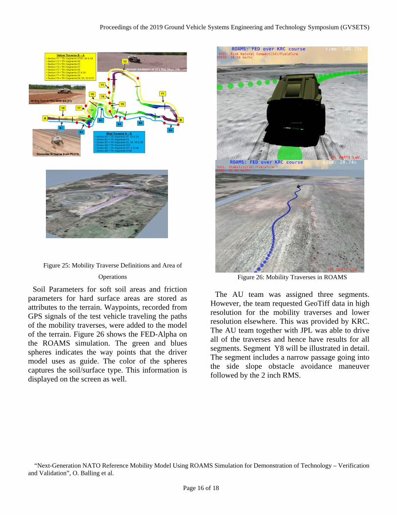
With the ROAMS simulation tool and using SimScape, the entire KRC Area of Operation was imported into the simulation framework. The definitions of the segments along with the entire area of operation loaded into ROAMS is illustrated in Figure 26.



of 18

Soil Parameters for soft soil areas and friction parameters for hard surface areas are stored as attributes to the terrain. Waypoints, recorded from GPS signals of the test vehicle traveling the paths of the mobility traverses, were added to the model of the terrain. Figure 26 shows the FED-Alpha on the ROAMS simulation. The green and blues spheres indicates the way points that the driver model uses as guide. The color of the spheres captures the soil/surface type. This information is displayed on the screen as well.

Figure 26: Mobility Traverses in ROAMS

The AU team was assigned three segments.

However, the team requested GeoTiff data in high resolution for the mobility traverses and lower resolution elsewhere. This was provided by KRC. The AU team together with JPL was able to drive all of the traverses and hence have results for all segments. Segment Y8 will be illustrated in detail. The segment includes a narrow passage going into the side slope obstacle avoidance maneuver followed by the 2 inch RMS.

Figure 25: Mobility Traverse Definitions and Area of

Operations



of 18

Figure 27: Mobility Traverse Segment Y8

The ROAMS simulation of segment Y8 is

compared to the actual vehicle test in Figure 28. The speed of the AU simulation is in general faster than the KRC test up until 200 meters traveled. This is because the simulated driver has less restriction with respect to speed than the actual driver sitting in the vehicle feeling the vibration levels. From approximately 210 to 310 meters traveled the vehicle is negotiating the side slop obstacle avoidance maneuver. The speed in test and simulation are comparable. The RMS course is also comparable as the RMS is limited by the 6 watt absorbed power speed. The two lower plots of Figure 28 show sideslip angle and lateral acceleration.

Figure 28: ROAMS Simulation of Segment Y8,

Comparison to Test

4. Conclusions and Discussions The ROAMS implementation and verification

and validation has shown its feasibility for the Next Generation-NATO Reference Mobility Model. A 3D multibody dynamics model was implemented in the software modeling framework ROAMS from JPL. The model was verified and validated against real test data. In the validation process, some discrepancies between the real tested vehicle and the simulated were identified. The major areas of disagreement is in the ride quality where the ROAMS simulation overestimated the speed for the half round and RMS course performance. Furthermore, it was proven difficult in its current form to model the Coarse Grain soil and the Fine Grain Sand Wet drawbar performance. However, the Fine Grain Sand Dry was possible to simulate using the Bekker Wong and Janosi terramechanics models. It appears that these models struggle to perform well on low bearing capacity soils evidenced by large rut depths. The uncertainty quantification was demonstrated using Go-NoGo and Speed-Made-Good confidence intervals by implementing 3D vehicle dynamics on soft soil to simulate uphill maximum speed or NoGo for a variation of soil and slope combinations. A surrogate model was generated by RAMDO Solutions to generate the confidence maps.

The mobility traverses were simulated using

KRC’s GeoTIFF terrain data based on high resolution scans of the segments and low resolution scans of the overall Area of Operation. The team has successfully implemented and demonstrated the vehicle based on the minimal coordinate formulation in ROAMS, the bulk terramechanics representation of the KRC soils and an automated speed and steering driver model using recorded waypoints as guidance. This enabled the team to fully automate the driving on both the yellow and blue traverses. Furthermore, at the CDT event in Houghton Michigan, September 25-27, the team demonstrated a realtime driving simulator capable of simulating the FED-Alpha vehicle dynamics on



of 18

soft and hard soil with a driver in the loop on the modeled KRC terrain traverses. Traverse speed versus distance traveled was compared to KRC testing. Other metrics were monitored for vehicle performance as well.

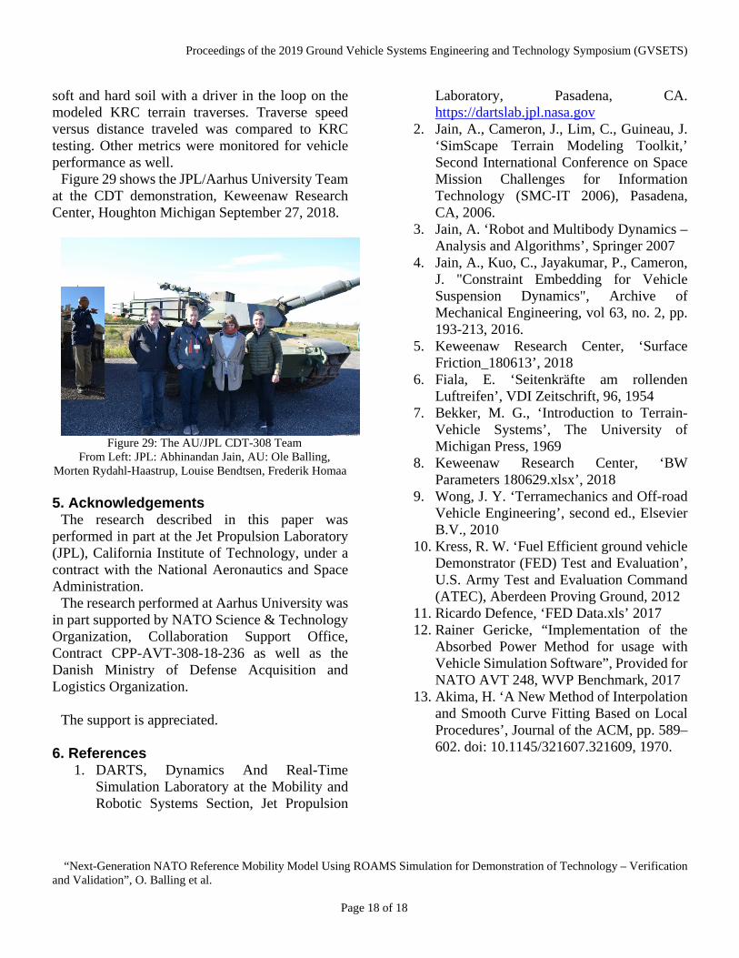
Figure 29 shows the JPL/Aarhus University Team at the CDT demonstration, Keweenaw Research Center, Houghton Michigan September 27, 2018.

Figure 29: The AU/JPL CDT-308 Team

From Left: JPL: Abhinandan Jain, AU: Ole Balling, Morten Rydahl-Haastrup, Louise Bendtsen, Frederik Homaa

5. Acknowledgements

The research described in this paper was performed in part at the Jet Propulsion Laboratory (JPL), California Institute of Technology, under a contract with the National Aeronautics and Space Administration.

The research performed at Aarhus University was in part supported by NATO Science & Technology Organization, Collaboration Support Office, Contract CPP-AVT-308-18-236 as well as the Danish Ministry of Defense Acquisition and Logistics Organization.

The support is appreciated.

6. References 1. DARTS, Dynamics And Real-Time

Simulation Laboratory at the Mobility and Robotic Systems Section, Jet Propulsion

Laboratory, Pasadena, CA. https://dartslab.jpl.nasa.gov

2. Jain, A., Cameron, J., Lim, C., Guineau, J. ‘SimScape Terrain Modeling Toolkit,’ Second International Conference on Space Mission Challenges for Information Technology (SMC-IT 2006), Pasadena, CA, 2006.

3. Jain, A. ‘Robot and Multibody Dynamics – Analysis and Algorithms’, Springer 2007

4. Jain, A., Kuo, C., Jayakumar, P., Cameron, J. "Constraint Embedding for Vehicle Suspension Dynamics", Archive of Mechanical Engineering, vol 63, no. 2, pp. 193-213, 2016.

5. Keweenaw Research Center, ‘Surface Friction_180613’, 2018

6. Fiala, E. ‘Seitenkräfte am rollenden Luftreifen’, VDI Zeitschrift, 96, 1954

7. Bekker, M. G., ‘Introduction to Terrain-Vehicle Systems’, The University of Michigan Press, 1969

8. Keweenaw Research Center, ‘BW Parameters 180629.xlsx’, 2018

9. Wong, J. Y. ‘Terramechanics and Off-road Vehicle Engineering’, second ed., Elsevier B.V., 2010

10. Kress, R. W. ‘Fuel Efficient ground vehicle Demonstrator (FED) Test and Evaluation’, U.S. Army Test and Evaluation Command (ATEC), Aberdeen Proving Ground, 2012

11. Ricardo Defence, ‘FED Data.xls’ 2017 12. Rainer Gericke, “Implementation of the

Absorbed Power Method for usage with Vehicle Simulation Software”, Provided for NATO AVT 248, WVP Benchmark, 2017

13. Akima, H. ‘A New Method of Interpolation and Smooth Curve Fitting Based on Local Procedures’, Journal of the ACM, pp. 589–602. doi: 10.1145/321607.321609, 1970.

https://dartslab.jpl.nasa.gov/

next-generation nato reference mobility model using …€¦ · generation nato reference mobility...

Documents