next performance curve analysis and validation€¦ · next performance curve analysis and...

NEXT Performance Curve Analysis And Validation

Pratik Saripalli∗

Graduate Research Assistant, College Park, Maryland, 20740, USA

Eric Cardiff† and Jacob Englander ‡

NASA Goddard Space Flight Center, Greenbelt, Maryland, 20770, USA

Performance curves of the NEXT thruster are highly important in determining thethruster’s ability in performing towards mission-specific goals. New performance curves areproposed and examined here. The Evolutionary Mission Trajectory Generator (EMTG)is used to verify variations in mission solutions based on both available thruster curvesand the new curves generated. Furthermore, variations in BOL and EOL curves are alsoexamined. Mission design results shown here validate the use of EMTG and the newperformance curves.

Nomenclature

m Mass flow rate, mg/sT Thrust, NIsp Specific impulse, secVbps Beam power supply voltage, VBOL Beginning of lifeEOL End of lifePin Input Power, kW

I. Introduction

Electric propulsion (EP) systems are required to perform within a wide range of requirements dependingon the mission. In order to accomplish this, proper performance characterization is required to understandeach thruster’s capabilities and limits for mission design analysis and evaluation.

NASA’s Evolutionary Xenon Thruster (NEXT) is a flight-qualified gridded electrostatic system that iscapable of offering two and a half times the thrust of the of the NSTAR ion engines.1 In order for it to beconsidered for future missions, its capabilities as an EP thruster must be quantified for mission planning,calling for a set of throttle curves that can characterize the thruster’s operating limits. These curves plotthe thrust (T) and mass flow rate (m) as a function of input power at constant beam power supply voltage(Vbsp). The Vbsp ranges from 275 V (low power) to 1800 V. The throttle table is shown in Table 1, below.Each Vbsp at a certain input power level is defined as a“throttle point”. Forty throttle points have beenidentified for NEXT, with each combination representing a unique beam voltage and current.2,3 NEXT hasbeen designed to operate between 0.6 - 7.2 kW input power. The throttle curves described in this paper aimto represent the performance capabilities of NEXT.

∗Graduate Research Assistant, Department of Aerospace Engineering, University of Maryland, College Park, 20740†Senior Propulsion Engineer, Propulsion Branch (CODE 597), NASA Goddard Space Flight Center‡Systems Engineer, Mission Design Branch (CODE 595), NASA Goddard Space Flight Center

1 of 30

https://ntrs.nasa.gov/search.jsp?R=20160009362 2020-04-29T20:47:58+00:00Z

Beam%Current,%A%

Beam%Power%Supply%Voltage%(Vbps),%V%

1800$ 1567$ 1396$ 1179$ 1021$ 936$ 850$ 700$ 679$ 650$ 400$ 300$ 275$

3.52$ TL40 TL39 TL38 TL37 ETL3.52A ETL3.52B ETL3.52C ETL3.52D $$ $$ $$ $$

3.10$ TL36 TL35 TL34 TL33 ETL3.1A ETL3.1B ETL3.1C ETL3.1D ETL3.1E $$ $$ $$

2.70$ TL32 TL31 TL30 TL29 TL28 ETL2.7A ETL2.7B ETL2.7C ETL2.7D ETL2.7E $$ $$



1.60$ TL17 TL16 TL15 TL14 TL13 ETL1.6A ETL1.6B ETL1.6C ETL1.6D ETL1.6E ETL1.6F

1.20$ TL12 TL11 TL10 TL09 TL08 TL07 TL06 $$ TL05 TL04 TL03 TL02

1.00$ TL01

Table 1: Input parameters for the throttle points available for the NEXT thruster.

NASA Glenn Research Center (GRC) has released high thrust and high Isp throttle curves that have beenused in mission designs for the Discovery and New Frontiers proposal calls. However, this paper suggeststhat these curves might not be adequate to accurately quantify the thruster’s performance. Trajectoryoptimizers use throttle curves to find the best solutions for a required mission objective. By not havingnumerous or accurate curves that can fully characterize a thruster, mission solutions won’t be fully optimized.Mission trajectories will vary depending on the thruster curve used, resulting in an inability to reproducean optimized solution. Furthermore, if degradation of thruster performance due to regular operation isn’taccounted for, more inaccuracies can occur. Therefore, validation of thruster curves is necessary for properthruster performance characterization. A global trajectory optimizer (such as EMTG, discussed later) isrequired to test each throttle curve against specific mission requirements.

II. Engine Models

A. New Throttle Curves

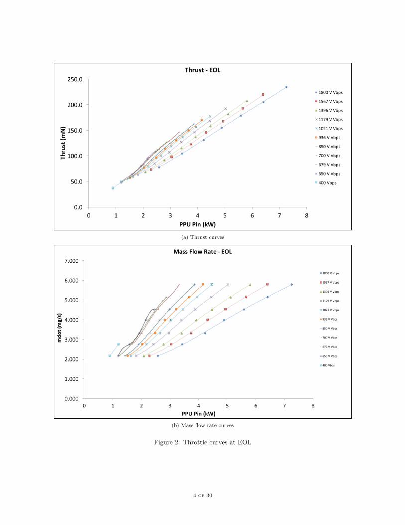
Each throttle point shown in Table 1 has documented beginning of life (BOL) and end of life (EOL)data describing m and T. Using these values, separate thruster curves were generated for each Vbsp at bothBOL and EOL. In order to have a continuous curve, a 4th-order polynomial best fit was applied to eachcurve. These curves can be found in the Appendix. None of the fit lines have a R2 value lower than 0.99,verifying good representation of the data. Furthermore, BOL and EOL high thrust and high Isp curves werealso generated using the highest thrust and m values at each Vbsp. Throughout the paper, the 1800 Vbsp

BOL and EOL curves along with the BOL and EOL high thrust curves were used to compare with the GRCcurves. Data was taken from Throttle Table 11, released by GRC.4

Figures 1 and 2 show the thruster curves for thrust and m at each Vbsp, BOL and EOL. Each plot includesthe discrete data points as well as the fit lines. Note that the lowest Vbsp fit line shown is 400 V. The 275Vbsp and 300 Vbsp fit lines are not shown for clarity purposes.

2 of 30

0.0

50.0

100.0

150.0

200.0

250.0

0 1 2 3 4 5 6 7 8

Thrust(m

N)

PPUPin(kW)

Thrust- BOL1800VVbps

1567VVbps

1396VVbps

1179VVbps

1021VVbps

936VVbps

850VVbps

700VVbps

679VVbps

650VVbps

400Vbps

(a) Thrust curves

0.000

1.000

2.000

3.000

4.000

5.000

6.000

7.000

0 1 2 3 4 5 6 7 8

mdo

t(mg/s)

PPUPin(kW)

MassFlowRate- BOL

1800VVbps

1567VVbps

1396VVbps

1179VVbps

1021VVbps

936VVbps

850VVbps

700VVbps

679VVbps

650VVbps

400Vbps

(b) Mass flow rate curves

Figure 1: Throttle curves at BOL

3 of 30

0.0

50.0

100.0

150.0

200.0

250.0

0 1 2 3 4 5 6 7 8

Thrust(m

N)

PPUPin(kW)

Thrust- EOL

1800VVbps

1567VVbps

1396VVbps

1179VVbps

1021VVbps

936VVbps

850VVbps

700VVbps

679VVbps

650VVbps

400Vbps

(a) Thrust curves

0.000

1.000

2.000

3.000

4.000

5.000

6.000

7.000

0 1 2 3 4 5 6 7 8

mdo

t(mg/s)

PPUPin(kW)

MassFlowRate- EOL

1800VVbps

1567VVbps

1396VVbps

1179VVbps

1021VVbps

936VVbps

850VVbps

700VVbps

679VVbps

650VVbps

400Vbps


Figure 2: Throttle curves at EOL

4 of 30

As can be seen in Figures 1 and 2, there are no data points to represent the low-power regime for thehigh voltage curves, especially for the 1800 V curve. This forces the polynomial fit to inaccurately representthe thrust and mass flow rate at low power. Therefore, data points from lower voltage curves were used togenerate modified fit-lines at 1800 V. These are shown below (Figures 3 and 4). The points shown in redrepresent the original 1800 V data whereas the points shown in blue represent the modified 1800 V data.It is clear that the modified curves have better representation of the low-power regime. In addition to themodified 1800 V curves, high thrust and high Isp curves were also generated. Table 2 visualizes the throttlepoints used for the hight thrust and high Isp curves as well as the modified 1800 V curves. The green linein Figure 2a shows the throttle points used for the high thrust curves. The red line in Figure 2b shows thethrottle points used for the high Isp curves. Figure 2b also shows the throttle points used for the modified1800 V curves, marked by the dashed yellow line. Figure 5 plots these new throttle curves alongside otherspreviously generated.

Before moving on, it is beneficial to address the validity of the approach used to generate the modified1800 V curves. The modified 1800 V curves use similar throttle points to the high Isp curves (see Table2b). The only difference is fewer points were used in defining the low power regime of the 1800 V curve.This was to ensure the modified 1800 V curve was still a predominantly 1800 Vbsp curve but still have somerepresentation in the low power regime. Therefore, the modified 1800 V curve is a hybrid between the full1800 V curve and a high Isp curve. Both of these curves, along with the curves mentioned above, were usedin the mission analysis discussed latter in the paper.

5 of 30

Beam%Current,%A%


1800$ 1567$ 1396$ 1179$ 1021$ 936$ 850$ 700$ 679$ 650$ 400$ 300$ 275$








1.00$ TL01

(a) High thrust curve throttle points

Beam%Current,%A%


1800$ 1567$ 1396$ 1179$ 1021$ 936$ 850$ 700$ 679$ 650$ 400$ 300$ 275$








1.00$ TL01

(b) High Isp (red) and 1800 V (dashed yellow) curve throttle points

Table 2: Throttle points used for the high thrust and high Isp curves

6 of 30

0.0

50.0

100.0

150.0

200.0

250.0

0 1 2 3 4 5 6 7 8

Thrust(m

N)

PPUPin(W)

Thrust- BOL

1800VVbpsBOL(Modified)

1800VVbpsBOL

(a) Thrust curves

0.000

1.000

2.000

3.000

4.000

5.000

6.000

7.000

0 1 2 3 4 5 6 7 8

mdo

t(mg/s)

PPUPin(kW)

MassFlowRate- BOL

1800VVbpsBOL(Modified)

1800VVbpsBOL


Figure 3: Throttle curves for 1800 V at BOL

7 of 30

0.0

50.0

100.0

150.0

200.0

250.0

0 1 2 3 4 5 6 7 8

Thrust(m

N)

PPUPin(kW)

Thrust- EOL

1800VVbpsEOL(Modified)

1800VVbpsEOL

(a) Thrust curves

0.000

1.000

2.000

3.000

4.000

5.000

6.000

7.000

0 1 2 3 4 5 6 7 8

mdo

t(mg/s)

PPUPin(kW)

MassFlowRate- EOL

1800VVbpsEOL(Modified)

1800VVbpsEOL


Figure 4: Throttle curves for 1800 V at EOL

8 of 30

0.0

50.0

100.0

150.0

200.0

250.0

0 1 2 3 4 5 6 7 8

Thrust(m

N)

PPUPin(kW)

HighThrustContour1800VVbps

1567VVbps

1396VVbps

1179VVbps

1021VVbps

936VVbps

850VVbps

700VVbps

679VVbps

650VVbps

(a) High thrust contour polynomial

0

500

1,000

1,500

2,000

2,500

3,000

3,500

4,000

4,500

0 1 2 3 4 5 6 7 8

Isp(sec)

PPUPin(kW)

HighISPContour

1800VVbps

1567VVbps

1396VVbps

1179VVbps

1021VVbps

936VVbps

850VVbps

700VVbps

679VVbps

650VVbps

400-275VVbps

(b) High Isp contour polynomial

Figure 5: Contour plots for high thrust and high Isp

9 of 30

B. GRC Curves

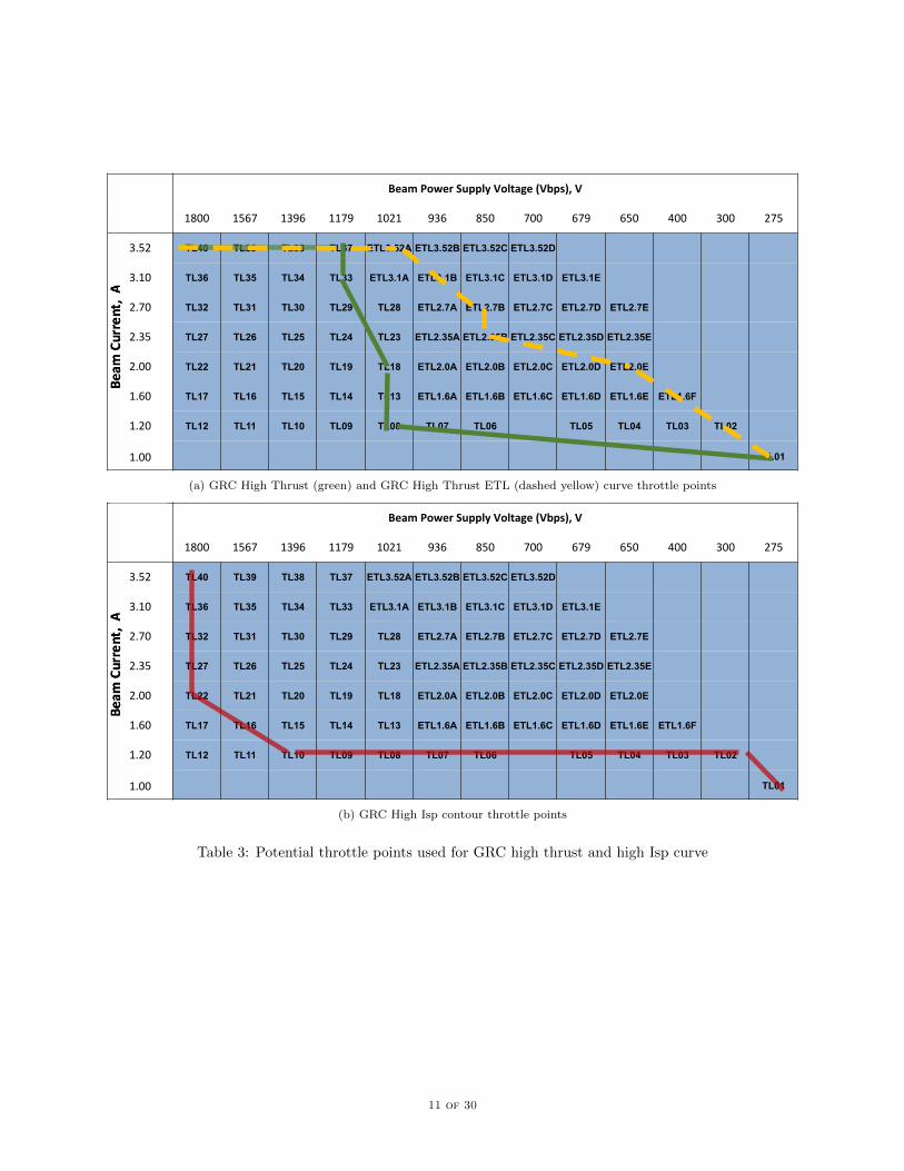
NASA GRC has documented multiple curve fits that are currently being used for mission analysis.According to the 2014 NEXT Discovery AO,4 the GRC high thrust curves are broken up into baselinethrottle level and an extended throttle level (ETL) curves. An effort has been made to extract whichthrottle points were used to generate the GRC high thrust and high Isp curves (Tables 3a and 3b).

The equations for all the fit lines are shown in Tables 9, 10, 11, and 12 located in the appendix section.The high Isp and high thrust equations are also listed. Tables 13, 14, 15 and 16 show the equations for GRChigh thrust and GRC high thrust ETL curves. The GRC high Isp equations are listed in Tables 17 and 18.Note that the independent variable for these equation is Pin.a.

aHigher significant figures were used for the 1800 Vbsp to ensure no error at full power

10 of 30

Beam%Current,%A%


1800$ 1567$ 1396$ 1179$ 1021$ 936$ 850$ 700$ 679$ 650$ 400$ 300$ 275$








1.00$ TL01

(a) GRC High Thrust (green) and GRC High Thrust ETL (dashed yellow) curve throttle points

Beam%Current,%A%


1800$ 1567$ 1396$ 1179$ 1021$ 936$ 850$ 700$ 679$ 650$ 400$ 300$ 275$








1.00$ TL01

(b) GRC High Isp contour throttle points

Table 3: Potential throttle points used for GRC high thrust and high Isp curve

11 of 30

C. Comparision

The following figures compare the GRC high thrust and high Isp curves with the author’s high thrustand high Isp curves (Figures 6 and 7). The black lines represent the high thrust and Isp curves generatedby the authors in this paper and the blue represent the baseline GRC high thrust and high Isp curves forNEXT. Specific to the high thrust plots, the red lines represent the GRC high thrust ETL curves.

The GRC high Isp curves and the author’s high Isp curves are relatively close to each other with someareas at which the thrust and mass flow rate curves vary slightly. It is expected that there will be smallvariations when using these curves for mission design, which will be addressed below. The high thrust curves,on the other hand, have a larger discrepancy between them. This paper’s high thrust curves used throttlepoints that maximized thrust (maximizing beam current at lower levels of beam power supply voltage). TheGRC and GRC ETL curves used throttle points with lower beam current levels at lower beam power supplyvoltage).

Figures 8 and 9, below, plot each of throttle curves on thrust vs input power and mass flow rate vs inputpower graphs. The curves are broken up into high thrust and high Isp categories. As is shown, there is somevariation between curves, especially between the GRC curves and the curves generated in this paper. Thesevariations do have an effect on mission planning as explored further in the paper.

In particular, in Figure 6 the high thrust curve produces the same amount of thrust as the GRC curvesat both ends of input power (low and high power) but higher thrust at powers from 1 kW to 6 kW. In Figure7, the 1800 V BOL/EOL curves are higher in thrust and lower in Isp than the GRC curves at low powerbut provide similar amounts of thrust at higher Isp’s at powers 2 kW to 5 kW. Figures 8 and 9 plot all thecurves used for mission analysis.

12 of 30

-50

0

50

100

150

200

250

0 1 2 3 4 5 6 7 8

Thrust(m

N)

PPUPin(kW)

HighThrustComparision(Thrust)

GRCHighThrust

GRCHighThrust(ETL)

Poly.(HighThrustContour)

(a) High Thrust Comparison (Thrust)

0

1

2

3

4

5

6

7

0 1 2 3 4 5 6 7 8

mdo

t(mg/s)

PPUPin(kW)

HighThrust(mdot)Comparision

GRCHighThrust

BOLHighThrust

GRCHighThrust(ETL)

(b) High Thrust Comparison (m-dot)

Figure 6: Comparison of High Thrust Equations

13 of 30

-50

0

50

100

150

200

250

300

0 1 2 3 4 5 6 7 8

Thrust(m

N)

PPUPin(kW)

HighIspComparison(Thrust)

GRCHighISP

BOLHighIsp

(a) High Isp Comparison (Thrust)

0

1

2

3

4

5

6

7

0 1 2 3 4 5 6 7 8

mdo

t(mg/s)

PPUPin(kW)

HighIspComparison

GlennHIGHISP

BOLHighISP

(b) High Isp Comparison (m-dot)

Figure 7: Comparison of High Isp Equations

14 of 30

-50

0

50

100

150

200

250

300

0 1 2 3 4 5 6 7 8

Thrust(m

N)

PPUPin(kW)

ComparisonPlot- HighThrust(Thrust)

GRCHighThrust

HighThrustBOL

HighThrustEOL

GRCHighThrust(ETL)

(a) High Thrust (thrust)

0

1

2

3

4

5

6

7

0 1 2 3 4 5 6 7 8

mdo

t(mg/s)

PPUPin(kW)

ComparisonPlot- HighThrust(mdot)

GRCHighThrust

HighThrustBOL

HighThrustEOL

GRCHighThrust(ETL)

(b) High Thrust (mdot)

Figure 8: Comparison plots for High Thrust

15 of 30

-50

0

50

100

150

200

250

300

0 1 2 3 4 5 6 7 8

Thrust(m

N)

PPUPin(kW)

ComparisonPlot- HighISP(Thrust)

1800BOL

1800EOL

GRCHighISP

HighIspBOL

HighIspEOL

(a) High Isp (thrust)

0

1

2

3

4

5

6

7

0 1 2 3 4 5 6 7 8

mdo

t(mg/s)

PPUPin(kW)

ComparisonPlot- HighISP(mdot)

1800BOL

1800EOL

GRCHighISP

HighIspBOL

HighIspEOL

(b) High Isp (mdot)

Figure 9: Comparison plots for High Isp

16 of 30

III. Mission Analysis

EMTG5 is an in-house NASA GSFC flight dynamics low thrust global optimizer that provides solutionsfor various mission criteria. Starting with user-inputs of thrust and mass flow rate curves, along with otherconstraints, EMTG produces a full mission solution. Therefore, by creating a custom mission using data-based thrust and mass flow rate curves, one can produce a better visual on the effects of the different curveson the thruster and mission.6–8

EMTG has previously been used in support of the OSIRIS-Rex Step 2 New Frontiers proposal andsubsequently for Phase C work on that mission. In addition, EMTG is being used to support the AsteroidRedirect Robotic Mission (ARRM).9 EMTGs low-thrust design capability is based on the medium-fidelitySims-Flanagan transcription and launch vehicle, and power system models5 which are industry standardfor this type of design. EMTGs modeling is therefore nearly identical to that employed in other industry-standard tools such as MALTO,10 GALLOP,11 PAGMO,12 and COLTT.13 Like other industry-standardtools, EMTG uses SPICE for all planetary and small-body ephemerides.14

A. Validation

The following paragraphs describe two classic test problems (DAWN and NEARER) from the literature15

which are relevant to small-body mission design. EMTG and MALTO, NASA Jet Propulsion Laboratory’s(JPL) equivalent tool, are used to provide missions solutions to these problems. These solutions are checkedfor consitency to help determine ensure EMTG’s validation.

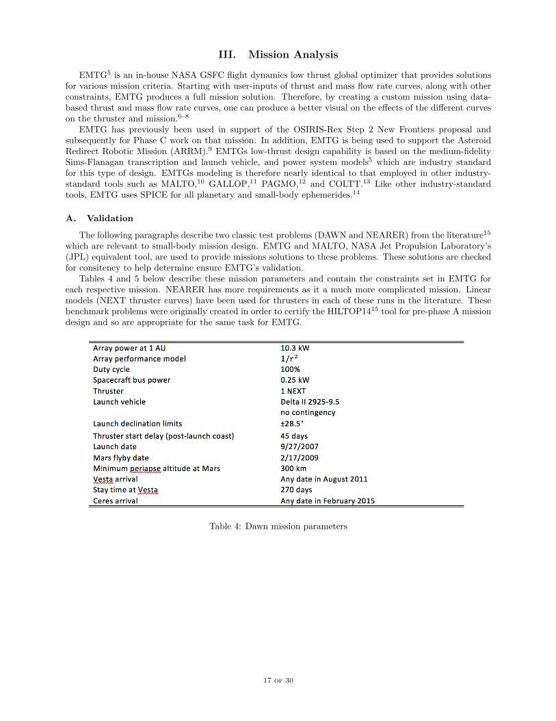
Tables 4 and 5 below describe these mission parameters and contain the constraints set in EMTG foreach respective mission. NEARER has more requirements as it a much more complicated mission. Linearmodels (NEXT thruster curves) have been used for thrusters in each of these runs in the literature. Thesebenchmark problems were originally created in order to certify the HILTOP1415 tool for pre-phase A missiondesign and so are appropriate for the same task for EMTG.

Table 4: Dawn mission parameters

17 of 30

Table 5: NEARER mission parameters

1. DAWN

The spacecraft (used in the mission optimizer) is identical to Dawn in all respects except that insteadof using the NSTAR thruster, it uses an early version of the NEXT thruster. Also, because the two toolsfor which the problem was originally constructed, HILTOP and MALTO, had different propulsion modelingschemes, the NEXT performance model is linearized as follows:

T = atP + bt

m = afP + bf

where T is thrust, m is mass flow rate, P is available power, and at is 7.282, bt = 32.901, af = 1.066 and bf= 0.699 are model coefficients.

The optimal solutions found using EMTG and MALTO are shown in Table 6. Note that the result foundby the two tools are nearly identical, well within the bounds of acceptability for preliminary design. Theonly difference is that EMTG was able to improve the propellant use by 0.8 kg by moving the Mars flybytwo weeks later than in the solution found using MALTO. This could be because of small (much less than 1percent) modeling differences between the two medium-fidelity tools or because of a small bifurcation in thesolution space where each tool went in a slightly different direction. The difference between the two solutionsis negligible. A plot of the optimal trajectory found in EMTG is shown in Figure 10. Note: this solution isvery similar to how all mission solutions are calculated throughout the paper.

18 of 30

Event Location Date C3 Mass

EMTG MALTO EMTG MALTO EMTG MALTO

Launch Earth 9/27/2007 9/27/2007 5.1529 5.1529 1114.4 1114.4

Flyby Mars 3/2/2009 2/18/2009 16.48 16.81 1040.2 1039.8Arrival Vesta 8/1/2011 8/1/2011 908.4 907.3

Departure Vesta 4/27/2012 4/27/2012 908.4 907.3

Arrival Ceres 2/28/2015 2/28/2015 808.0 807.2

Table 6: Comparison of the EMTG and MALTO solutions to the Dawn test problem

Figure 10: Optimal EMTG solution to the Dawn test problem

19 of 30

2. NEARER

The optimal solutions found by EMTG and MALTO are shown in Table 7. Two EMTG solutions arepresented. The first solution forces EMTG to produce the same solution as MALTO. The solutions werevery close: 808.7 kg final mass for EMTG vs 810.2 kg for MALTO, a difference of 0.2%.

This solution results in a violation of the propellant tank constraint by 1.5 kg. The small difference isdue to the slight differences in modeling between the two tools and is not significant for preliminary design.After the first solution was found, EMTG was allowed to search the solution space more thoroughly andlook for solutions that meet the constraints originally set but are not necessarily similar to the publishedMALTO trajectory. EMTGs global search mode identified a solution with a launch date in October 2014instead of the published May 2014. This launch date enables a more efficient Earth to Nereus phase whichallows a final mass of 830.5 kg. The optimal solution is shown in Figure 11.

Event Location Date C3 MassEMTG#1 EMTG#2 MALTO EMTG

#1EMTG#2

MALTO EMTG#1 EMTG#2 MALTO

Launch Earth 5/15/14 10/3/14 5/17/14 39.9 39.3 39.9 1312.2 1332.8 1312.2

Arrival Nereus 6/22/16 6/20/16 6/24/16 1125.4 1150.4 1129.3

Departure Nereus 8/21/16 8/19/16 8/23/16 1090.4 1115.4 1094.3

Flyby Earth 2/1/18 2/3/18 2/4/18 39.2 39.6 44.5 960.2 986.4 963.7Arrival 1996FG3 5/14/20 5/6/20 6/4/20 891.7 915.5 893.0

Departure 1996FG3 8/1/20 7/27/20 8/3/20 861.7 885.5 863.0

Arrival Earth 6/21/21 6/21/21 6/21/21 44.9 44.9 44.9 808.7 830.8 810.2

Table 7: Comparison of the EMTG and MALTO solutions to the NEARER test problem

Figure 11: Optimal solution to the NEARER test problem

The examples presented above demonstrate that EMTGs modeling fidelity is sufficient for preliminarydesign and is equivalent, if not superior, to the commonly used MALTO tool. The differences between

20 of 30

EMTGs modeling and that of other medium-fidelity tools are significantly less than the difference betweenany medium-fidelity design and the eventual high-fidelity design.

B. EMTG Customization

Customization for EMTG is broken up into three categories: global mission options, spacecraft optionsand journey options. The global mission parameter options include mission launch dates, duration boundsand locations of launch. Spacecraft options primarily deal with power and propulsion of the mission. Thelaunch vehicle as well as the thruster can be changed. Custom thruster curves can also be input to thesystem. Power sources for the spacecraft can either be solar or radioisotope. A power model and a decayrate can also be implemented.

In this work, an Earth to Mars mission was designed as a control to test each of the throttle curves inEMTG. It was a 3 year mission with a 30 day launch date window. A successful mission scenario occurswhen the spacecraft launches from Earth, reaches rendezvous with Mars and performs a “spiral down”landing procedure. All parameters are set constant when changing between different throttle curves. Table8 contains this information. Three optimization variables were chosen for EMTG. They were maximizingpayload mass, minimizing time (final mass constraint set), and minimizing BOL power (reducing the size ofthe solar array).

Table 8: EMTG contraints: Earth to Mars

C. Results

In the following tables, the modified 1800 V curves from both the BOL and EOL along with theirrespective high thrust curves are being compared to the NASA GRC high thrust (baseline and ETL) andIsp curves. Figure 12 compares the high Isp curves with the 1800 V BOL and EOL modified curves. FigureFigures 13 compares the high thrust curves. Tables 19, 20, and 21 (Appendix A) present the data collectedfrom EMTG for each optimization.

Figures 12a, 12b, and 12c present results from the high ISP curves and 1800 V curves. Figure 12a displayshow much propellant was used during each mission. For solutions optimized for maximizing final mass, the1800 V BOL curves used the least amount of propellant where as the EOL high ISP curve and GRC highISP curves used the most amount of propellant. The solutions vary by a few kg’s of propellant, which isstill significant for such a small mission. When optimizing for minimum time, all missions used the sameamount of propellant due to a final mass constraint (mentioned above). The maximum propellant allowablefor this mission was 125 kg (525 kg (initial mass) - 400 kg (maximum final mass)). This helps further solidifyEMTG’s ability to implement mission constraints into its optimization scheme. Lastly, when looking atminimizing BOL power, the BOL/EOL high Isp curves used the most amount of propellant.

Figure 12b shows the total trip time for all optimization (for high Isp curves). For all three optimizations,the total trip time only varies by tens of days between each curve. Figure 12c shows the peak power generated(right after launch) for each of the three optimizations. Once again, there isn’t a large difference betweeneach of the curves for peak power generated. The GRC high Isp curve does necessitate a slightly larger solararray when minimizing for BOL power.

The high thrust curves shown in Figures 13a, 13b and 13c show that the GRC high thrust curve used theleast amount of propellant when maximizing final mass to produce similar trip times which is counter-intuitivesince a high thrust curve should use more propellant to achieve shorter trip times. This is addressed in thediscussion section below. The GRC ETL curve used about the same amount of propellant as the BOL/EOLhigh thrust curves. All of the high thrust curves used the same amount of propellant when optimizing for

21 of 30

minimum time and minimum BOL power. The high thrust curves also had very similar trip times for eachoptimization.

When looking at peak power generated (Figure 13c), there is variation when the curves were optimizingtowards minimum BOL power. The GRC curves have a higher peak power than the other curves, failing tominimize BOL power.

22 of 30

70

80

90

100

110

120

130

140

150

MaximizingFinalMass MinimizingTime MinimizingBOLpower

Prop

ellentUsed(kg)

EarthtoMars:PropellantUsed(HighISPContours)

1800VBOL 1800VEOL GRCISP BOLHighISP EOLHighISP

(a) High ISP curves - comparing propellant used

0

100

200

300

400

500

600

700

800


TripTim

e(days)

EarthtoMars:TripTime(HighISPContours)


(b) High ISP curves - comparing total trip time

0

2

4

6

8

10

12


PeakPow

erGen

erated

(kW)

EarthtoMars:PeakPowerGenerated(MinimizingBOLPower,HighIspContours)


(c) High ISP curves - comparing peak power used

Figure 12: Earth to Mars results: High Isp

23 of 30

70

80

90

100

110

120

130

140

150


Prop

ellentUsed(kg)

EarthtoMars:PropellantUsed(HighThrustContours)

GRCHighThrust(ETL) GRCHighThrust BOLHighThrust EOLHighThrust

(a) High thrust curves - comparing propellant used

0

100

200

300

400

500

600

700

800


TripTim

e(days)

EarthtoMars:TripTime(HighThrustContours)

GRCHighThrust(ETL) GRCHighThrust BOLHighThrust EOLHighThrust

(b) High thrust curves - comparing total trip time

0

2

4

6

8

10

12

MaximizingFinalMass MinimizingTime

PeakPow

erGen

erated

(kW)

EarthtoMars:PeakPowerGenerated(MinimizingBOLPower,HighThrustContours)

GlennHighThrust(ETL) GRCHighThrust BOLHighThrust EOLHighThrust

(c) High thrust curves - comparing comparing peak power used

Figure 13: Earth to Mars results: High Thrust

24 of 30

IV. Discussion

There are two specific findings of note within the high thrust solutions. The first is propellant usagewhen optimizing for maximum final mass (Figure 13a). The GRC high thrust curve produced similar triptimes as the other curves when maximizing final mass but required much less propellant. This is because theGRC high thrust curve uses only the regular throttle points instead of the extended throttle table, allowingEMTG to access the lower power levels of NEXT. Therefore, the GRC high thrust curve has a higher Ispthan the GRC ETL curve, resulting in a solution that didn’t require as much propellant.

The second discrepancy within the high thrust curve solutions occurs when optimizing for BOL power(Figure 13c). The GRC high thrust curve requires almost 0.8 kW more power (when compared to other highthrust curves) in a case that minimizes BOL power. The GRC high thrust ETL curve and the BOL/EOLhigh thrust curves developed here provide the best results for a power-constrained mission.

The GRC high Isp curves performed relatively well when compared to the high Isp curves created here.Most of the solutions required similar amounts of propellant and total trip time. When optimizing formaximum final mass, the GRC high Isp curve falls between the BOL and EOL curve for high Isp. Similarly,it fell in between the 1800 V BOL and EOL curve for propellant usage when minimizing BOL power.

The reason why the high thrust curves differ more than the high Isp curves is due to the throttle pointsthe GRC curves seem to be generated from. The GRC high Isp curve (Figure ??) use almost the samethrottle points as BOL/EOL high Isp curves (Figure ??) except at low beam current levels (at 1800 beampower supply voltage). Such a small difference resulted in only small variations between mission solutions.The high thrust curves, on the other hand, have more noticeable variations between mission solutions. Thisis due to the GRC high thrust and GRC high thrust ETL curves using throttle points (Figure ??) that don’tfully maximized towards high thrust (when compared to the BOL/EOL high thrust curves shown in Figure??).

In general, the new curves generated here for thrust produce lower trip time solutions and the high Ispcurves produce lower propellant required solutions when compared to the GRC high thrust and high Ispcurves. In each of the tests, results have differed on the order of days for trip time and kg’s for propellant.Specific to the Earth to Mars mission, on average, propellant variation is around 10 kg between two extremes.When optimizing for maximizing final mass, as shown in Figures 12a and 13c, this would be more than a 10percent change in propellant use. Although the percent change on the overall trip time between curves isn’tas high with only a few days variation against an overall trip time that is a few hundreds of days (Figures12b and 13b), it does represent mission solution variations that need to be accounted for.

In addition to differences between BOL/EOL and GRC curves, it is shown that BOL and EOL donot produce the same results in any scenario, indicating the effect of thruster degradation, as mentionedpreviously. Improvements to this would require an interpolation method in order to properly address anyperformance decrease of the thruster, which currently does not exist. Nevertheless, a single curve is notsufficient to describe thruster performance as demonstrated by the difference in mission solutions among theBOL, EOL and GRC curves.

V. Conclusion

From the work done in this paper, it is seen that existing curves for NEXT are not sufficient to characterizeits performance. Optimal performance of a given mission was characterized by propellant mass, total triptime and peak-power (size of solar array). The GRC high thrust and high Isp curves do not fully maximizethrust and Isp respectively. Small variations between the GRC curves and the ones generated in thispaper result in different solutions to an optimized mission-design. For high thrust, curves that follow theETL perform better for power-constrained missions and the non-ETL high thrust curves perform better forpropellant constrained missions. Furthermore, thruster degradation needs to be accounted for as well.

Acknowledgments

The authors would like to thank the Harriett Jenkins Graduate Fellowship for funding this research aswell as Mike Patterson for consulting on the throttle table.

25 of 30

References

1Garner, R., “NASA’s Goddard, Glenn Centers Look to Lift Space Astronomy out of the Fog,” March 2012, [Online;posted 03-March-2012].

2Soulas, C. G. and Patterson, M. J., “NEXT Ion Thruster Performance Dispersion Analyses,” .3Herman, D. A., Soulas, G. C., Van Noord, J. L., and Patterson, M. J., “NASAs Evolutionary Xenon Thruster Long-

Duration Test Results,” Journal of Propulsion and Power , Vol. 28, No. 3.4“NEXT Document for Discovery 2014 AO Library,” .5Englander, J. A., Ellison, D. H., and Conway, B. A., “Global Optimization of Low-Thrust, Multiple-Flyby Trajectories

at Medium and Medium-High Fidelity,” .6Englander, J. A., Vavrina, M. A., Naasz, B., Merill, R. G., and Qu, M., “Mars, Phobos, and Deimos Sample Return

Enabled by ARRM Alternative Trade Study Spacecraft,” .7Englander, J., Automated Trajectory Planning For Multiple-Flyby Interplanetary Missions, Ph.D. thesis, University of

Illinois at Urbana-Champaign, Illinois, 2013.8Englander, J. A. and Englander, A. C., “Tuning Monotonic Basin Hopping: Improving the Efficiency of Stochastic Search

as Applied to Low-Thrust Trajectory Optimization,” .9Englander, J., Vavrina, M., Naasz, B., Merill, R., and Qu, M., “Mars, Phoos, and Deimos Sample Return Enabled by

ARRM Alternative Trade Study Spacecraft,” .10Sims, J. A., Finlayson, P., Rinderle, E., Vavrina, M., and Kowalkowski, T., “Implementation of a low-thrust trajectory

optimization algorithm for preliminary design,” .11McConaghy, T., Debban, T., Petropolous, A., and Longuski, J., “Design and Optimization of Low-Thrust Trajectories

with Gravity Assists,” Journal of Spacecraft and Rockets, Vol. 40.12Yam, C., Di Lorenzo, D., and Izzo, D., “Low-Thrust Trajectory Design as a Constrained Global Optimization Problem,”

Part G: Journal of Aerospace Engineering, Vol. 225.13Herman, J., Zimmer, A., Reijneveld, J., Dunlop, K., Takahashi, Y., Tardivel, S., and Scheeres, D., “Human Exploration

of Near Earth Asteroids: Mission Analysis for a Chemical and Electric Propulsion Mission,” Acta Astronautica.14“Spice Ephemeris,” DOI: 10.1016/j.actaastro.2014.07.034.15Horsewood, Jerry, L. and Dankanich, J. W., “Heliocentric Interplanetary Low-thrust Trajectory Optimization Program

Capabilities and Comparison to NASAs Low-thrust Trajectory Tools,” .

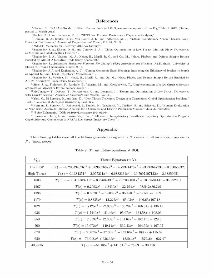
Appendix

The following tables show all the fit lines generated along with GRC curves. In all instances, x representsPin (input power).

Table 9: Thrust fit-line equations at BOL

Vbsp Thrust Equation (mN)

High ISP T (x) = −0.200394396x4 + 3.09602667x3 − 14.79371475x2 + 53.24364773x− 0.880568326

High Thrust T (x) = 0.13843514 − 2.057211x3 + 6.6882331x2 + 39.7097107132x− 2.38859651

1800 T (x) = −0.041430321x4 + 0.2968243x3 + 2.37060001x2 + 10.5258144x + 34.992831

1567 T (x) = 0.2593x4 − 4.8436x3 + 32.794x2 − 58.542x86.249

1396 T (x) = 0.3078x4 − 5.5039x3 + 35.458x2 − 58.533x81.189

1179 T (x) = 0.8335x4 − 12.225x3 + 65.03x2 − 106.65x107.18

1021 T (x) = 1.7125x4 − 22.389x3 + 105.28x2 − 166.54x + 136.17

936 T (x) = 1.7449x4 − 21.46x3 + 95.07x2 − 134.58x + 108.06

850 T (x) = 2.87924 − 32.368x3 + 131.64x2 − 182.47x + 129.3

700 T (x) = 15.072x4 − 149.14x3 + 539.43x2 − 794.55x + 467.02

679 T (x) = 3.3676x4 − 37.335x3 + 143.66x2 − 180.2x + 115.69

650 T (x) = −76.018x4 + 536.65x3 + −1380.4x2 + 1579.2x− 627.97

400-275 T (x) = −54.185x3 + 141.54x2 − 75.69x + 30.498

26 of 30

Table 10: Mass flow rate fit-line equations at BOL

Vbsp Mass Flow Rate (mg/s)

High ISP m(x) = −0.005987542x4 + 0.074628525x3 − 0.175668526x2 + 0.151098815x + 1.956250894

High Thrust m(x) = 0.0084761x4 − 0.1113601x3 + 0.2587433x2 + 1.44382383x + 0.7717598

1800 m(x) = −0.00266205x4 + 0.0150629x3 + 0.20069186x2 − 0.83824381x + 2.8759130

1567 m(x) = 0.0118x4 − 0.2377x3 + 1.712x2 − 4.2632x + 5.3694

1396 m(x) = 0.0161x4 − 0.3012x3 + 2.0117x2 − 4.5961x + 5.3217

1179 m(x) = 0.0355x4 − 0.5574x3 + 3.1474x2 − 6.2963x + 6.0651

1021 m(x) = 0.0812x4 − 1.0969x3 + 5.3349x2 − 9.6331x + 7.762

936 m(x) = 0.0873x4 − 1.0939x3 + 4.9409x2 − 8.0383x + 6.2311

850 m(x) = 0.1266x4 − 1.4707x3 + 6.1652x2 − 9.42x + 6.6949

700 m(x) = 1.0409x4 − 10.375x3 + 37.864x2 − 57.984x + 34.106

679 m(x) = 0.0535x4 − 0.0992x3 + 2.0944x2 − 3.3188x + 3.2846

650 m(x) = −5.6594x4 + 40.367x3 − 105.1x2 + 120.06x− 48.65

400-275 m(x) = −17.475x3 − 45.14x2 + 38.754x2 − 9.0094

Table 11: Thrust fit-line equations at EOL

Vbsp Thrust Equation (mN)

High ISP T (x) = −0.196896539x4 + 3.05918604x3 − 14.72524921x2 + 53.32445536x− 1.335725134

High Thrust T (x) = 0.13701397x4 − 2.05900345x36.8929834x2 + 38.74487882x + 2.250668

1800 T (x) = −0.0405432x4 + 0.29083768x3 + 2.3320396x2 + 10.6571918x + 34.687332

1567 T (x) = 0.2534x4 − 4.7545x3 + 32.34x2 − 57.84x + 85.831

1396 T (x) = 0.2996x4 − 5.3855x3 + 34.883x2 − 57.68x + 80.699

1179 T (x) = 0.809x4 − 11.937x3 + 63.874x2 − 105.15x + 106.51

1021 T (x) = 1.6564x4 − 21.802x3 + 103.2x2 − 164.07x + 135.23

936 T (x) = 1.6806x4 − 20.82x3 + 92.899x2 − 132.08x + 107.07

850 T (x) = 2.7668x4 − 31.346x3 + 128.46x2 − 179.06x + 128.09

700 T (x) = 14.355x4 − 143.34x3 + 523.13x2 − 776.89x + 460.99

679 T (x) = 3.2213x4 − 36.011x3 + 139.76x2 − 176.44x + 114.53

650 T (x) = −71.839x4 + 511.84x3 − 1328.6x2 + 1534.5x− 615.39

400-275 T (x) = −59.967x3 + 158.93x2 − 92.693x + 35.411

27 of 30

Table 12: Mass flow rate fit-line equations at EOL

Vbsp Mass Flow Rate (mg/s)

High ISP m(x) = −0.004792385x4 + 0.057358188x3 − 0.09987237x2 + 0.032353523x + 2.137689593

High Thrust m(x) = 0.0094585x4 − 0.12660861x3 + 0.3336997x2 + 1.3059342x + 0.9485779

1800 m(x) = −0.001156113x4 − 0.00786841x3 + 0.31217985x2 − 1.0476175x + 3.1343462

1567 m(x) = 0.0086x4 − 0.1704x3 + 1.2174x2 − 2.7769x + 3.9603

1396 m(x) = 0.0113x4 − 0.2107x3 + 1.4067x2 − 2.9458x + 3.9006

1179 m(x) = 0.0265x4 − 0.4128x3 + 2.3166x2 − 4.3433x + 4.6092

1021 m(x) = 0.0479x4 − 0.6627x3 + 3.3035x2 − 5.6585x + 5.1535

936 m(x) = 0.0682x4 − 0.8811x3 + 4.104x2 − 6.6825x + 5.5781

850 m(x) = 0.0995x4 − 1.1913x3 + 5.1458x2 − 7.8876x + 6.0038

700 m(x) = 0.967x4 − 9.7669x336.14x2 − 56.095x + 33.612

679 m(x) = −0.0909x4 + 0.2654x3 + 0.8749x2 − 1.6774x + 2.6339

650 m(x) = −5.6776x4 + 40.975x3 + −107.97x2 + 124.74x− 51.056

400-275 m(x) = 16.961x3 − 44.401x2 + 38.632x− 8.9972

Table 13: GRC high thrust thrust fit-line equations4

Thrust (mN)

GRC thrustT (x) = 0.101855017x4 − 2.04053417x3

+ 11.4181412x2 + 16.0989424x + 11.9388817

Table 14: GRC high thrust mass flow rate fit-line equations4

Mass Flow Rate (mg/s)

GRC mdotm(x) = 0.011021367x4 − 0.207253445x3

+ 1.216702370x2 − 1.71102132x + 2.75956482

Table 15: GRC high thrust (ETL) thrust fit-line equations4

Thrust (mN)

GRC ETL thrustT (x) = 0.085120672x4 − 1.42659172x3

+ 5.17797704x2 + 37.1873936x + −0.804281458

28 of 30

Table 16: GRC high thrust (ETL) mass flow rate fit-line equations4


GRC mdotm(x) = 0.009019519x4 − 0.138009326x3

+ 0.535910391x20.534442545x + 1.40535083

Table 17: GRC high Isp thrust fit-line equations4

Thrust (mN)

GRC thurstT (x) = −0.111563126x4 + 1.72548416x3

+ −7.91621814x2 + 40.543251x + 3.68945763

Table 18: GRC high Isp mass flow rate fit-line equations4


GRC mdotT (x) = −0.00291399146x4 + 0.0298873982000000x3

+ 0.0277715756x2 − 0.180919262x + 2.22052155

29 of 30

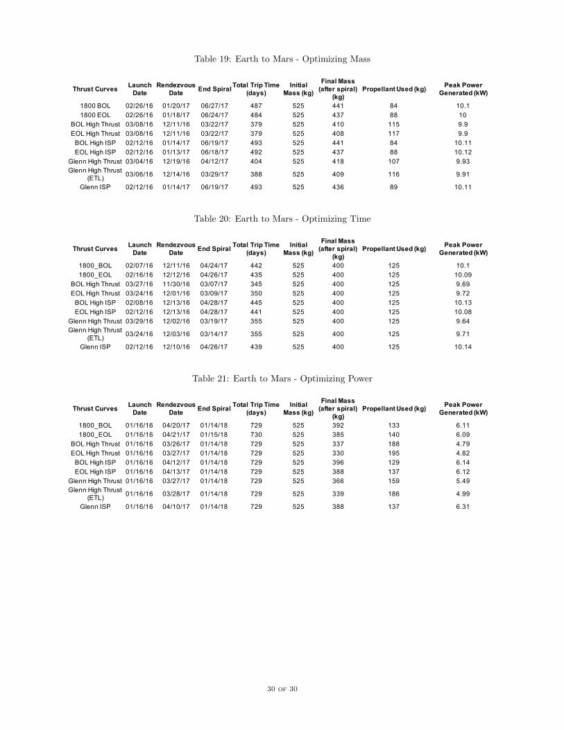
Table 19: Earth to Mars - Optimizing Mass

Thrust Curves Launch Date

Rendezvous Date End Spiral Total Trip Time

(days)Initial

Mass (kg)

Final Mass (after spiral)

(kg)Propellant Used (kg) Peak Power

Generated (kW)

1800 BOL 02/26/16 01/20/17 06/27/17 487 525 441 84 10.11800 EOL 02/26/16 01/18/17 06/24/17 484 525 437 88 10

BOL High Thrust 03/08/16 12/11/16 03/22/17 379 525 410 115 9.9EOL High Thrust 03/08/16 12/11/16 03/22/17 379 525 408 117 9.9

BOL High ISP 02/12/16 01/14/17 06/19/17 493 525 441 84 10.11EOL High ISP 02/12/16 01/13/17 06/18/17 492 525 437 88 10.12

Glenn High Thrust 03/04/16 12/19/16 04/12/17 404 525 418 107 9.93Glenn High Thrust

(ETL) 03/06/16 12/14/16 03/29/17 388 525 409 116 9.91

Glenn ISP 02/12/16 01/14/17 06/19/17 493 525 436 89 10.11

Table 20: Earth to Mars - Optimizing Time



(days)Initial

Mass (kg)



Generated (kW)

1800_BOL 02/07/16 12/11/16 04/24/17 442 525 400 125 10.11800_EOL 02/16/16 12/12/16 04/26/17 435 525 400 125 10.09




(ETL) 03/24/16 12/03/16 03/14/17 355 525 400 125 9.71

Glenn ISP 02/12/16 12/10/16 04/26/17 439 525 400 125 10.14

Table 21: Earth to Mars - Optimizing Power



(days)Initial

Mass (kg)



Generated (kW)

1800_BOL 01/16/16 04/20/17 01/14/18 729 525 392 133 6.111800_EOL 01/16/16 04/21/17 01/15/18 730 525 385 140 6.09




(ETL) 01/16/16 03/28/17 01/14/18 729 525 339 186 4.99

Glenn ISP 01/16/16 04/10/17 01/14/18 729 525 388 137 6.31

30 of 30

next performance curve analysis and validation€¦ · next performance curve analysis and...

Documents