next-to-leading order in qcd
TRANSCRIPT

arX
iv:h
ep-p
h/02
0308
9v1
8 M
ar 2
002
RM3-TH/02-3ROME1-1333/02
SHEP 02/04
Lifetime Ratios of Beauty Hadrons at the
Next-to-Leading Order in QCD
E. Francoa, V. Lubiczb, F. Mesciac and C. Tarantinob
a Dip. di Fisica, Univ. di Roma “La Sapienza” and INFN, Sezione di Roma,
P.le A. Moro 2, I-00185 Rome, Italy
b Dip. di Fisica, Univ. di Roma Tre and INFN, Sezione di Roma III,
Via della Vasca Navale 84, I-00146 Rome, Italy
c Dept. of Physics and Astronomy, Univ. of Southampton,
Highfield, Southampton, SO17 1BJ, U.K.
Abstract
We compute the next-to-leading order QCD corrections to spectator effects in thelifetime ratios of beauty hadrons. With respect to previous calculations, we take intoaccount the non vanishing value of the charm quark mass. We obtain the predictionsτ(B+)/τ(Bd) = 1.06±0.02, τ(Bs)/τ(Bd) = 1.00±0.01 and τ(Λb)/τ(Bd) = 0.90±0.05,in good agreement with the experimental results. In the case of τ(Bs)/τ(Bd) andτ(Λb)/τ(Bd), however, some contributions, which either vanish in the vacuum inser-tion approximation or represent a pure NLO corrections, have not been determinedyet.

1 Introduction
The inclusive decay rates of beauty hadrons can be computed by expanding the amplitudesin increasing powers of ΛQCD/mb [1, 2] and using the assumption of quark-hadron duality.The leading term in this expansion reproduces the predictions of the naıve quark spectatormodel, and the first correction of O(1/mb) is absent in this case.
Within this theoretical framework, up to terms of O(1/m2b) only the b quark enters
the short-distance weak decay, while the light quarks in the hadron interact through softgluons only. For this reason, the lifetime ratios of beauty hadrons are predicted to be unityat this order, with corrections which are at most of few percent.
Spectator contributions, which are expected to be mainly responsible for the lifetimedifferences of beauty hadrons, only appear at O(1/m3
b) in the Heavy Quark Expansion(HQE). These effects, although suppressed by powers of 1/mb, are enhanced, with respectto leading contributions, by a phase-space factor of 16π2, being 2 → 2 processes instead of1 → 3 decays. Indeed, the inclusion of these corrections at the leading order (LO) in QCDhas allowed to reproduce the observed pattern of the lifetime ratios [3, 4].
In this paper we compute the next-to-leading order (NLO) QCD corrections to spectatoreffects in the lifetime ratios of beauty hadrons. In the limit of vanishing charm quark mass,these corrections have been already computed in ref. [5], and we refer to this paper for manydetails of the NLO calculation. We find that the inclusion of the NLO corrections improvesthe agreement with the experimental measurements. Moreover, it increases the accuracyof the theoretical predictions by reducing significantly the dependence on the operatorrenormalization scale.
After our calculation was completed, the NLO corrections to spectator effects in theratio τ(B+)/τ(Bd) have been also presented in ref. [6]. We agree with their results. Withrespect to ref. [6], we also perform in this paper the NLO calculation of the Wilson coeffi-cients entering the HQE of the ratios τ(Bs)/τ(Bd) and τ(Λb)/τ(Bd).
By using the lattice determinations of the relevant hadronic matrix elements [7]-[10],we have performed a theoretical estimate of the lifetime ratios and obtained the NLOpredictions
τ(B+)
τ(Bd)= 1.06± 0.02 ,
τ(Bs)
τ(Bd)= 1.00± 0.01 ,
τ(Λb)
τ(Bd)= 0.90± 0.05 . (1)
These estimates must be compared with the experimental measurements [11]
τ(B+)
τ(Bd)= 1.074± 0.014 ,
τ(Bs)
τ(Bd)= 0.948± 0.038 ,
τ(Λb)
τ(Bd)= 0.796± 0.052 . (2)
The theoretical predictions turn out to be in good agreement with the experimental data.As we will discuss below, however, in the case of τ(Bs)/τ(Bd) and τ(Λb)/τ(Bd) the theo-retical predictions can be further improved, since some contributions, which either vanishin the vacuum insertion approximation (VIA) or represent a pure NLO correction, are stilllacking. With respect to the results of ref. [5], we find that the NLO charm quark masscorrections are rather large for some of the Wilson coefficients. Nevertheless, the totaleffect of these contributions on the lifetime ratios is numerically small.
1

An important check of the perturbative calculation performed in this paper is providedby the cancellation of the infrared (IR) divergences in the expressions of the Wilson co-efficients, in spite these divergences appear in the individual amplitudes. The presenceof these divergences explicitly shows that the Bloch-Nordsieck theorem does not apply innon-abelian gauge theories [12]-[14]. We have also checked that our results are explicitlygauge invariant and have the correct ultraviolet (UV) renormalization-scale dependence aspredicted by the known LO anomalous dimensions of the relevant operators.
The HQE of the lifetime ratios results in a series of local operators of increasing dimen-sion defined in the Heavy Quark Effective Theory (HQET). Indeed, renormalized operatorsin QCD mix with operators of lower dimension, with coefficients proportional to powersof the b-quark mass. In this case, the dimensional ordering of the HQE would be lost. Inorder to implement the expansion, the matrix elements of the local operators should becut-off at a scale smaller than the b-quark mass, which is naturally realized in the HQET.1
In the case of τ(B+)/τ(Bd), only flavour non-singlet operators enter the expansion. Forthese operators, the mixing with lower dimensional operators is absent, and the HQE canbe expressed in terms of operators defined in QCD. For these operators, the matchingbetween QCD and HQET has been computed, at the NLO, in ref. [5].
As mentioned before, the NLO predictions for the lifetime ratios τ(Bs)/τ(Bd) andτ(Λb)/τ(Bd) may still be improved in some ways. In particular:
- the contributions of the four-fermion operators containing the charm quark field andof the penguin operator (see eqs. (10) and (11)) have not been determined yet. Thesecontributions, which either vanish in the VIA (charm operators) or represent a pureNLO correction (penguin operator), do not affect the theoretical determination ofτ(B+)/τ(Bd) and represent only an SU(3)-breaking effect for τ(Bs)/τ(Bd);
- the lattice determination of the hadronic matrix elements have been performed byneglecting penguin contractions (i.e. eye diagrams), which exist in the case of flavoursinglet operators. Also in this case, the corresponding contributions cancel in theratio τ(B+)/τ(Bd) but affect τ(Λb)/τ(Bd) and τ(Bs)/τ(Bd), the latter only throughSU(3)-breaking effects;
- the NLO anomalous dimension of the four-fermion DB = 0 operators in the HQETis still unknown. For this reason, the renormalization scale evolution of the Λb matrixelements, computed on the lattice in the HQET at a scale smaller than the b-quarkmass [8, 9], has been only performed at the LO. For B mesons, a complete NLOevolution has been performed by using operators defined in QCD [10].
For these reasons, at present, the best theoretical accuracy is achieved in the determinationof the lifetime ratio τ(B+)/τ(Bd).
We conclude this section by presenting the plan of this paper. In sect. 2 we review thebasic formalism of the HQE applied to the lifetime ratios of beauty hadrons. Details of theNLO calculation and the numerical results obtained for the Wilson coefficients are givenin sect. 3. In sect. 4 we present the predictions for the lifetime ratios of beauty hadrons.
1On this point, we disagree with the general statement of ref. [6] according to which the HQE can beperformed in QCD also in the presence of mixing with lower dimensional operators.
2

Finally, we collect in the appendix the analytical expressions for the Wilson coefficientfunctions.
2 HQE for the lifetime ratios of beauty hadrons
Using the optical theorem, the inclusive decay width Γ(Hb) of a hadron containing a bquark can be written as
Γ(Hb) =1
MHb
Im〈Hb|T |Hb〉 , (3)
where the transition operator T is given by
T = i∫
d4x T(H∆B=1
eff (x)H∆B=1eff (0)
)(4)
and H∆B=1eff is the effective weak hamiltonian which describes ∆B = 1 transitions.
By neglecting the Cabibbo suppressed contribution of b → u transitions (|Vub|2/|Vcb|2 ∼0.16λ2) and terms proportional to |Vtd|/|Vts| in the penguin sector, the ∆B = 1 effectivehamiltonian can be written in the form
H∆B=1eff =
GF√2V ∗
cb
[C1 (Q1 +Qc
1)+C2 (Q2 +Qc2)+
6∑
i=3
CiQi+C8GQ8G+∑
l=e,µ,τ
Ql
]+h.c. . (5)
The Ci are the Wilson coefficients, known at the NLO in perturbation theory [15]-[17], andthe operators Qi are defined as
Q1 = (bicj)V−A(ujd′
i)V−A , Q2 = (bici)V−A(ujd′
j)V−A ,
Qc1 = (bicj)V−A(cjs
′
i)V−A , Qc2 = (bici)V−A(cjs
′
j)V−A ,
Q3 = (bisi)V−A
∑
q
(qjqj)V−A , Q4 = (bisj)V−A
∑
q
(qjqi)V−A ,
Q5 = (bisi)V−A
∑
q
(qjqj)V+A , Q6 = (bisj)V−A
∑
q
(qjqi)V+A ,
Q8G =gs8π2
mbbiσµν (1− γ5) taijsjG
aµν , Ql = (bici)V−A(νll)V−A ,
(6)
where d ′ = cos θcd + sin θcs and s ′ = − sin θcd + cos θcs (θc is the Cabibbo angle). Hereand in the following we use the notation (qq)V±A = qγµ(1±γ5)q and (qq)S±P = q(1±γ5)q.A sum over repeated colour indices is always understood.
Because of the large mass of the b quark, it is possible to construct an Operator ProductExpansion (OPE) for the transition operator T of eq. (4), which results in a sum of localoperators of increasing dimension [1, 2]. We include in this expansion terms up to O(1/m2
b)plus those 1/m3
b corrections that come from spectator effects and are enhanced by the phasespace. The resulting expression for the inclusive width of eq. (3) is given by
Γ(Hb) =G2
F |Vcb|2m5b
192π3
c(3)
〈bb〉Hb
2MHb
+ c(5)gsm2
b
〈bσµνGµνb〉Hb
2MHb
+96π2
m3b
∑
k
c(6)k
〈O(6)k 〉Hb
2MHb
, (7)
3
b b 1 b b
b b 1/mb2
b b
b b
s s
1/mb3
b b
s s
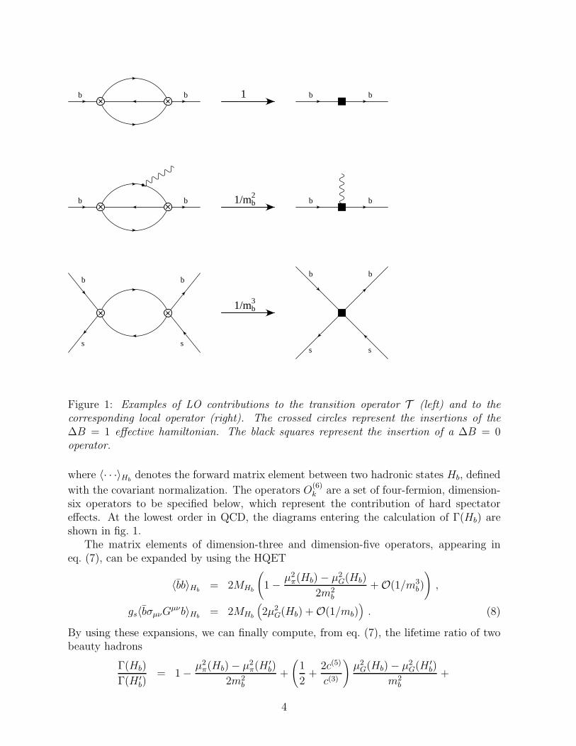
Figure 1: Examples of LO contributions to the transition operator T (left) and to thecorresponding local operator (right). The crossed circles represent the insertions of the∆B = 1 effective hamiltonian. The black squares represent the insertion of a ∆B = 0operator.
where 〈· · ·〉Hbdenotes the forward matrix element between two hadronic states Hb, defined
with the covariant normalization. The operators O(6)k are a set of four-fermion, dimension-
six operators to be specified below, which represent the contribution of hard spectatoreffects. At the lowest order in QCD, the diagrams entering the calculation of Γ(Hb) areshown in fig. 1.
The matrix elements of dimension-three and dimension-five operators, appearing ineq. (7), can be expanded by using the HQET
〈bb〉Hb= 2MHb
(1− µ2
π(Hb)− µ2G(Hb)
2m2b
+O(1/m3b)
),
gs〈bσµνGµνb〉Hb
= 2MHb
(2µ2
G(Hb) +O(1/mb)). (8)
By using these expansions, we can finally compute, from eq. (7), the lifetime ratio of twobeauty hadrons
Γ(Hb)
Γ(H ′
b)= 1− µ2
π(Hb)− µ2π(H
′
b)
2m2b
+
(1
2+
2c(5)
c(3)
)µ2G(Hb)− µ2
G(H′
b)
m2b
+
4

96π2
m3b c
(3)
∑
k
c(6)k
〈O(6)
k 〉Hb
2MHb
−〈O(6)
k 〉H′
b
2MH′
b
. (9)
The dimension-six operators in eq. (9), which express the hard spectator contributions,are the four current-current operators2
Oq1 = (b q)V−A (q b)V−A , Oq
2 = (b q)S−P (q b)S+P ,
Oq3 = (b taq)V−A (q tab)V−A , Oq
4 = (b taq)S−P (q tab)S+P ,
(10)
with q = u, d, s, c, and the penguin operator
OP = (btab)V∑
q=u,d,s,c
(qtaq)V . (11)
In these definitions, the symbols b and b denote the heavy quark fields in the HQET.The Wilson coefficients c(3) and c(5), of the dimension-three and dimension-five operators
in eq. (9), have been computed at the LO in ref. [18], while the NLO corrections to c(3) havebeen evaluated in [19]-[24]. The NLO corrections to c(5) are still missing. Their numericalcontribution to the lifetime ratios, however, is expected to be negligible.
The coefficient functions of the dimension-six current-current operators Oqk, have been
computed at the LO in ref. [4, 25] for q = u, d, s, and in ref. [26] for q = c. The coefficientfunction of the penguin operator OP vanishes at the LO.
In this paper we have computed the NLO QCD corrections to the coefficient func-tions of the operators Oq
k with q = u, d, s. The operators containing the charm quarkfields contribute, as valence operators, only to the inclusive decay rate of Bc mesons, andtheir contribution to non-charmed hadron decay rates is expected to be negligible. Thecalculation of the NLO corrections to these coefficient functions, as well as the NLO cal-culation of the coefficient function of the penguin operator, has not been performed yet.The non-perturbative determinations of the corresponding matrix elements are also lack-ing at present. However, as we will discuss in sect. 4, these contributions only enter thetheoretical estimates of the ratios τ(Bs)/τ(Bd) and τ(Λb)/τ(Bd), and vanish in the VIA.
3 NLO calculation of the Wilson coefficients
All the details of the matching procedure used to determine the Wilson coefficients atthe NLO have been given in ref. [5], where the calculation has been performed in thelimit of vanishing charm quark mass. A finite value of the charm quark mass does notintroduce conceptual difficulties in the calculation, besides requiring the evaluation of one-and two-loop integrals with an additional mass scale. For this reason, we only remind inthis section the general strategy of the perturbative calculation, and refer the interestedreader to ref. [5] for further details. In this section, we will also present the numericalresults for the Wilson coefficients, while the analytical expressions of these coefficients arecollected in the appendix.
5

b
q
b
q
D1
b
q
b
q
D2
b
q
b
q
D3
b
q
b
q
D4
b
q
b
q
D5
b
q
b
q
D6
b
q
b
q
D7
b
q
b
q
D8
b
q
b
q
D9
b
q
b
q
D10
b
q
b
q
D11
b
q
b
q
D12
b
q
b
q
D13
b
q
b
q
D14
b
q
b
q
D15
Figure 2: Feynman diagrams which contribute at NLO to the matrix element of the tran-sition operator T in the case q = s. In the other cases, q = u, d, diagrams D14 and D15
are Cabibbo suppressed and have been neglected in the calculation.
6

b
q
b
qE1
b
q
b
qE2
b
q
b
qE3
b
q
b
qE4
b
q
b
qE5
b
q
b
qE6
Figure 3: Feynman diagrams which contribute, at NLO, to the matrix element of the ∆B =0 operators entering the HQET.
In order to compute the Wilson coefficients of the ∆B = 0 operators at the NLO, wehave evaluated in QCD the imaginary part of the diagrams shown in fig. 2 (full theory) andin the HQET the diagrams shown in fig. 3 (effective theory). The external quark stateshave been taken on-shell and all quark masses, except mb and mc, have been neglected.More specifically, we have chosen the heavy quark momenta p2b = m2
b in QCD and kb = 0 inthe HQET, and pq = 0 for the external light quarks. In this way, we automatically retainthe leading term in the 1/mb expansion. We have performed the calculation in a genericcovariant gauge, in order to check the gauge independence of the final results. Two-loopintegrals have been reduced to a set of independent master integrals by using the recurrencerelation technique [27]-[29] implemented in the TARCER package [30]. Equations of motionhave been used to reduce the number of independent operators.
Some diagrams, both in the full and in the effective theory, are plagued by IR diver-gences. These divergences do not cancel in the final partonic amplitudes, and provide anexample of violation of the Bloch-Nordsieck theorem in non-abelian gauge theories [12]-[14]. IR poles, however, are expected to cancel in the matching and we have explicitlychecked that, in the computation of the coefficient functions, this cancellation takes place.
We use D-dimensional regularization with anticommuting γ5 (NDR) to regularize bothUV and IR divergences. As discussed in details in ref. [5], the presence of dimensionally-regularized IR divergences introduces subtleties in the matching procedure. The matchingmust be consistently performed in D dimensions. This requires, in particular, enlarging
2Note that, with respect to ref. [5], we use a different basis of operators.
7

the operator basis to include (renormalized) evanescent operators, which must be insertedin the one-loop diagrams of the effective theory. Because of the IR divergences, the matrixelements of the renormalized evanescent operators do not vanish in the D → 4 limit [31],and give a finite contribution in the matching procedure.
As a check of the perturbative calculation, we have verified that our results for theWilson coefficients satisfy the following requirements:
• gauge invariance: the coefficient functions in the MS scheme are explicitly gauge-invariant. The same is true for the full and the effective amplitudes separately;
• renormalization-scale dependence: the coefficient functions have the correct logarith-mic scale dependence as predicted by the LO anomalous dimensions of the ∆B = 0and ∆B = 1 operators;
• IR divergences: the coefficient functions are infrared finite. We verified that thecancellation of IR divergences also takes place, separately in the full and the effectiveamplitudes, for the abelian combination of diagrams .
The ∆B = 0 effective theory is derived from the double insertion of the ∆B = 1 effectivehamiltonian. Therefore, the coefficient functions cqk of the ∆B = 0 effective theory dependquadratically on the coefficient functions Ci of the ∆B = 1 effective hamiltonian, and wecan write
cqk(µ0) =∑
i,j
Ci(µ1)Cj(µ1)Fqk,ij(µ1, µ0) . (12)
Eq. (12) shows explicitly the scale dependence of the several terms. We denote with µ1 therenormalization scale of the ∆B = 1 effective hamiltonian, whereas µ0 is the renormaliza-tion scale of the ∆B = 0 operators. The coefficients F q
k,ij depend on the renormalizationscheme and scale of both the ∆B = 0 and ∆B = 1 operators. The dependence on the scaleµ1 and on the renormalization scheme of the ∆B = 1 operators actually cancels, order byorder in perturbation theory, against the corresponding dependence of the ∆B = 1 Wilsoncoefficients Ci. Therefore, the coefficient functions cqk only depend on the renormalizationscheme and scale of the ∆B = 0 operators. We have chosen to renormalize these operators,in the HQET, in the NDR-MS scheme defined in details in ref. [32].
The four fermion operators, in the effective ∆B = 1 hamiltonian, are naturally ex-pressed in terms of the weak eigenstates d ′ and s ′. For this reason, we can write thecoefficients F q
k,ij of eq. (12) in the form
F dk,ij = cos2 θcF
d ′
k,ij + sin2 θcFs ′
k,ij
F sk,ij = sin2 θcF
d ′
k,ij + cos2 θcFs ′
k,ij (13)
for i, j = 1, 2. In the case q = s, the coefficient functions also receive contributions fromthe insertion of the penguin and chromomagnetic operators (diagram D15 of fig. 2). Sincethe Wilson coefficients C3–C6 are small, contributions with a double insertion of penguinoperators can be safely neglected. As suggested in [33], a consistent way for implementingthis approximation is to consider the coefficients C3–C6 as formally of O(αs). Within thisapproximation, only single insertions of penguin operators need to be considered at the
8

q = d q = u q = s
LO NLO NLO LO NLO NLO LO NLO NLO
(mc = 0) (mc = 0) (mc = 0)
c q1 −0.02 −0.03 −0.03 −0.06 −0.33 −0.29 −0.01 −0.03 −0.03
c q2 0.02 0.03 0.03 0.00 −0.01 −0.01 0.02 0.03 0.04
c q3 −0.70 −0.65 −0.67 2.11 2.27 2.34 −0.61 −0.51 −0.56
c q4 0.79 0.68 0.68 0.00 −0.06 −0.05 0.77 0.61 0.64
Table 1: Wilson coefficients cqk computed at the LO and NLO, in the latter case with andwithout the inclusion of charm quark mass corrections at O(αs). As reference values of theinput parameters, we use µ0 = µ1 = mb = 4.8 GeV and mc = 1.4 GeV.
NLO, and we can write
csk =∑
i,j=1,2
CiCjFsk,ij + 2
αs
4πC2C8GPk,28 + 2
∑
i=1,2
∑
r=3,6
Ci CrPk,ir , (14)
which generalizes eq. (12) for the case q = s.The analytical expressions of the coefficients F q
k,ij and Pk,ij will be given in the appendix.For illustration we present here, in table 1, the numerical values of the coefficients cqk bothat LO and NLO and, in the latter case, with and without the inclusion of the O(αs)charm quark mass corrections computed in this paper. As reference values of the inputparameters, we use µ0 = µ1 = mb = 4.8 GeV and mc = 1.4 GeV.
By looking at the results shown in table 1, we see that the NLO charm quark masscorrections are rather large for some of the Wilson coefficients, although the total effectof these contributions on the lifetime ratios will be found to be small. The numerical ex-pressions of the lifetime ratios as a function of the B-parameters will be given in the nextsection (eq.(26)). In these expressions we will also include an estimate of the theoreticalerror on the coefficients, coming from the residual NNLO dependence on the renormal-ization scale µ1 and from the uncertainties on the values of the charm and bottom quarkmasses and the other input parameters.
The combinations cuk−cdk (k = 1, . . . 4) of Wilson coefficients, which enter the theoreticalexpression of the ratio τ(B+)/τ(Bd), have been also computed, at the NLO, in ref. [6]. Inthis case, the corresponding operators are the flavour non-singlet combinations Ou
k − Odk,
which do not mix, with coefficients proportional to powers of the b quark mass, withoperators of lower dimension. For this reason, the HQE can be also expressed in this casein terms of operators defined in QCD, and this is the choice followed by ref. [6].
9

In order to compare our results with those of ref. [6], at the NLO, it is necessary toimplement the matching, at O(αs), between QCD and HQET operators. This matchingcan be written in terms of the Wilson coefficients, in the form
[cuk (mb)− c d
k (mb)]QCD
=
(1 +
αs(mb)
4πS
)
k,l
[cul (mb)− c d
l (mb)]HQET
, (15)
where a common renormalization scale µ = mb has been chosen for all the coefficients.The matrix S has been computed in ref. [5]. It depends on the renormalization schemes ofboth QCD and HQET operators. In this paper, we have chosen to renormalize the HQEToperators in the NDR-MS scheme of ref. [32]. By choosing for the QCD operators theNDR-MS scheme of ref. [6], defined in ref. [34], one finds that the matrix S is given by 3
S =
32/3 0 22/9 1/3
−16/3 −16/3 4/9 −2/9
11 3/2 −7/2 1/4
2 −1 3 5/2
(16)
By using eq. (15), we have verified that our results for the combinations cuk − cdk agreewith those of ref. [6]. Note that in the notation of [6] the labels u and d are interchangedwith respect to our convention and that the Wilson coefficients are defined with a relativefactor of 3. The numerical comparison of our results with those shown in table 1 of ref. [6],however, shows some differences, particularly at the LO. The reason is that some of thecoefficient functions, because of large cancellations, are extremely sensitive to the value ofthe coupling constant αs(µ).
4 Theoretical estimates of the lifetime ratios
In this section we present the theoretical estimates of the lifetime ratios of beauty hadrons,obtained by using the NLO expressions of the Wilson coefficients and the lattice determi-nations of the relevant hadronic matrix elements [7]-[10].
The HQE for the ratio of inclusive widths of beauty hadrons is expressed by eq. (9), upto and including 1/m3
b spectator effects. The combinations of hadronic parameters enteringthis formula at order 1/m2
b can be evaluated from the heavy hadron spectroscopy [35], andone obtains the estimate
τ(B+)
τ(Bd)= 1.00−∆B+
spec ,τ(Bs)
τ(Bd)= 1.00−∆Bs
spec ,τ(Λb)
τ(Bd)= 0.98(1)−∆Λ
spec , (17)
where the ∆s represent the 1/m3b contributions of hard spectator effects
∆Hbspec =
96π2
m3b c
(3)
∑
k
c(6)k
〈O(6)
k 〉Hb
2MHb
− 〈O(6)k 〉Bd
2MBd
. (18)
3This matrix differs from the matrix C1 given in ref. [5] by a linear transformation, since a basis of
operators different from eq. (10) has been chosen in that paper. More specifically, S = −MCT1M−1, where
M is defined in ref. [5].
10

Note that, by neglecting these contributions, the 1/m2b predictions of eq. (17) are incom-
patible with the experimental results of eq. (2).In parametrizing the matrix elements of the dimension-six current-current operators,
we follow the analysis of ref. [5] and we distinguish two cases, depending on whether ornot the light quark q of the operator enters as a valence quark in the external hadronicstate. Correspondingly, we introduce different B-parameters for the valence and non-valence contributions. For the B-meson matrix elements, we write the matrix elements ofthe non-valence operators in the form
〈Bq|Oq′
k |Bq〉2MBq
=f 2BqMBq
2δ q′qk for q 6= q′ , (19)
while, in the case of the valence contributions (q = q′), we write
〈Bq|Oq1|Bq〉
2MBq
=f 2BqMBq
2(B q
1 + δ qq1 ) ,
〈Bq|Oq3|Bq〉
2MBq
=f 2BqMBq
2(ε q
1 + δ qq3 ) ,
〈Bq|Oq2|Bq〉
2MBq
=f 2BqMBq
2(B q
2 + δ qq2 ) ,
〈Bq|Oq4|Bq〉
2MBq
=f 2BqMBq
2(ε q
2 + δ qq4 ) .
(20)
The parameters δ qqk in eq. (20) are defined as the δ qq′
k of eq. (19) in the limit of degeneratequark masses (mq = mq′). In the VIA, B q
1 = B q2 = 1 while the ε parameters and all the
δs vanish. Note that, in the SU(2) limit, the parameters B d1,2 and ε d
1,2 express the matrixelements of the non-singlet operator Ou
k −Odk between external B-meson states.
The reason to distinguish between valence and non valence contributions, is that onlythe former have been computed so far by using lattice QCD simulations [7, 10]. A non-perturbative lattice calculation of the δ parameters would be also possible, in principle.However, it requires to deal with the difficult problem of subtractions of power-divergences,which has prevented so far the calculation of the corresponding diagrams.
To complete the definitions of the B-parameters for the B-mesons, we introduce aparameter for the matrix element of the penguin operator
〈Bq|OP |Bq〉2MBq
=f 2BMB
2P q . (21)
We now define the B-parameters for the Λb baryon. Up to 1/mb corrections, the matrixelements of the operators Oq
2 and Oq4, between external Λb states, can be related to the
matrix elements of the operators Oq1 and Oq
3 [4]
〈Λb|Oq1|Λb〉 = −2 〈Λb|Oq
2|Λb〉 , 〈Λb|Oq3|Λb〉 = −2 〈Λb|Oq
4|Λb〉 . (22)
For the independent matrix elements, assuming SU(2) symmetry, we define
〈Λb|Oq1|Λb〉
2MΛb
=f 2BMB
2
(L1 + δ Λq
1
)for q = u, d ,
〈Λb|Oq3|Λb〉
2MΛb
=f 2BMB
2
(L2 + δ Λq
2
)for q = u, d ,
11

〈Λb|Oq1|Λb〉
2MΛb
=f 2BMB
2δ Λq1 for q = s, c , (23)
〈Λb|Oq3|Λb〉
2MΛb
=f 2BMB
2δ Λq2 for q = s, c ,
〈Λb|OP |Λb〉2MΛb
=f 2BMB
2P Λ .
In analogy with the B-meson case, the parameters L1 and L2 represent the valence contri-butions computed so far by current lattice calculations [8, 9].
In terms of valence and non valence B-parameters, the quantities ∆Hbspec of eq. (18),
which represent the spectator contributions to the lifetime ratios, are expressed in theform
∆B+
spec = 48π2 f2BMB
m3bc
(3)
4∑
k=1
(cuk − c d
k
)B dk ,
∆Bs
spec = 48π2 f2BMB
m3bc
(3)
{4∑
k=1
[r c s
k B sk − c d
k B dk +
(cuk + c d
k
) (r δ ds
k − δ ddk
)+
c sk
(r δ ss
k − δ sdk
)+ c c
k
(r δ cs
k − δ cdk
)]+ cP
(rP s − P d
)}, (24)
∆Λspec = 48π2 f
2BMB
m3bc
(3)
{4∑
k=1
[(cuk + c d
k
)LΛ
k − c dk B d
k +(cuk + c d
k
) (δ Λdk − δ dd
k
)+
c sk
(δ Λsk − δ sd
k
)+ c c
k
(δ Λck − δ cd
k
)]+ cP
(P Λ − P d
)}.
where r denotes the ratio (f 2BsMBs
)/(f 2BMB) and, in order to simplify the notation, we
have defined the vectors of parameters
~Bq = {Bq1, B
q2, ε
q1, ε
q1} ,
~L = {L1,−L1/2, L2,−L2/2} , (25)
~δΛq = {δΛq1 ,−δΛq1 /2, δΛq2 ,−δΛq2 /2} .
An important consequence of eq. (24) is that, because of the SU(2) symmetry, the non-valence (δs) and penguin (P s) contributions cancel out in the expressions of the lifetimeratio τ(B+)/τ(Bd). Thus, the theoretical prediction of this ratio is at present the mostaccurate, since it depends only on the non-perturbative parameters actually computed bycurrent lattice calculations. The prediction of the ratio τ(Λb)/τ(Bd), instead, is affectedby both the uncertainties on the values of the δ and P parameters, and by the unknownexpressions of the Wilson coefficients c c
k and cP at the NLO. For the ratio τ(Bs)/τ(Bd)the same uncertainties exist, although their effect is expected to be smaller, since thecontributions of non-valence and penguin operators cancel, in this case, in the limit ofexact SU(3) symmetry.
In the numerical analysis of the ratios τ(Bs)/τ(Bd) and τ(Λb)/τ(Bd), we will neglectthe non-valence and penguin contributions. The non-valence contributions vanish in theVIA, and present phenomenological estimates indicate that the corresponding matrix el-ements are suppressed, with respect to the valence contributions, by at least one order
12

of magnitude [36, 37]. On the other hand, the matrix elements of the penguin operatorsare not expected to be smaller than those of the valence operators. Since the coefficientfunction cP vanishes at the LO, this contribution is expected to have the size of a typicalNLO corrections. Thus, from a theoretical point of view, a quantitative evaluation of thenon-valence and penguin operator matrix elements would be of the greatest interest toimprove the determination of the ΛB lifetime.
By neglecting the non valence and penguin contributions, we obtain from eq. (24) thefollowing numerical expressions for the spectator effects
∆B+
spec = − 0.06(2)Bd1 − 0.010(3)Bd
2 + 0.7(2) εd1 − 0.18(5) εd2 ,
∆Bsspec = − 0.010(2)Bs
1 + 0.011(3)Bs2 − 0.16(4) εs1 + 0.18(5) εs2
+0.008(2)Bd1 − 0.008(2)Bd
2 + 0.16(4) εd1 − 0.16(4) εd2 ,
∆Λspec = − 0.08(2)L1 + 0.33(8)L2
+0.008(2)Bd1 − 0.008(2)Bd
2 + 0.16(4) εd1 − 0.16(4) εd2 ,
(26)
These formulae, which are accurate at the NLO, represent the main result of this paper.The errors on the coefficients take into account both the residual NNLO dependence onthe renormalization scale of the ∆B = 1 operators and the theoretical uncertainties onthe input parameters. To estimate the former, the scale µ1 has been varied in the intervalbetween mb/2 and 2mb. For the charm and bottom quark masses, and the B meson decayconstants we have used the central values and errors given in table 2. The strong couplingconstant has been fixed at the value αs(mZ) = 0.118. The parameter c(3) in eq. (24) isa function of the ratio m2
c/m2b , and such a dependence has been consistently taken into
account in the numerical analysis and in the estimates of the errors. For the range ofmasses given in table 2, c(3) varies in the interval c(3) = 3.4÷ 4.2 [22]-[24].
As discussed in the previous section, the HQE for the ratio τ(B+)/τ(Bd) can be alsoexpressed in terms of operators defined in QCD. The corresponding coefficient functionscan be evaluated by applying the matching defined in eq. (15). In this way, we obtain theexpression
∆B+
spec = − 0.05(1) Bd1 − 0.007(2) Bd
2 + 0.7(2) εd1 − 0.15(4) εd2 (27)
where the B and ε parameters are now defined in terms of matrix elements of QCD oper-ators. This expression is in agreement with the result obtained in ref. [6].
The errors quoted on the coefficients in eq. (26) are strongly correlated, since theyoriginate from the theoretical uncertainties on the same set of input parameters. For thisreason, in order to evaluate the lifetime ratios, we have not used directly eq. (26). Instead,we have performed a bayesian statistical analysis by implementing a short Monte Carlocalculation. The input parameters have been extracted with flat distributions, assumingas central values and standard deviations the values given in table 2. The results for theB-parameters are based on the lattice determinations of refs. [7]-[10].4 As discussed indetails in ref. [5], we have included in the errors an estimate of the uncertainties not taken
4For recent estimates of these matrix elements based on QCD sum rules, see refs. [38]-[41].
13

Bd1 = 1.2± 0.2 Bs
1 = 1.0± 0.2
Bd2 = 0.9± 0.1 Bs
2 = 0.8± 0.1
εd1 = 0.04± 0.01 εs1 = 0.03± 0.01
εd2 = 0.04± 0.01 εs2 = 0.03± 0.01
L1 = −0.2 ± 0.1 L2 = 0.2± 0.1
mb = 4.8± 0.1 GeV mb −mc = 3.40± 0.06 GeV
fB = 200± 25 MeV fBs/fB = 1.16± 0.04
Table 2: Central values and standard deviations of the input parameters used in the nu-merical analysis. The values of mb and mc refer to the pole mass definitions of thesequantities.
into account in the original papers. The QCD results for the B meson B-parameters ofref. [10] have been converted to HQET by using eq. (15).5 The contributions of all the δand P parameters have been neglected.
In this way we obtain the NLO predictions for the lifetimes ratios which have been alsoquoted in the introduction
τ(B+)
τ(Bd)= 1.06± 0.02 ,
τ(Bs)
τ(Bd)= 1.00± 0.01 ,
τ(Λb)
τ(Bd)= 0.90± 0.05 . (28)
The central values and errors correspond to the average and the standard deviation of thetheoretical distributions. These distributions are shown in fig. 4, together with the experi-mental ones. We mention that uncertainties coming from the residual scale dependence inthe results of eq. (28) represent less than 20% of the quoted errors.
In conclusion we find that, with the inclusion of the NLO corrections, the theoreticalprediction for the ratio τ(B+)/τ(Bd) turns out to be in very good agreement with the ex-perimental measurement, given in eq. (2). For the ratios τ(Bs)/τ(Bd) and τ(Λb)/τ(Bd) theagreement is also very satisfactory, and the difference between theoretical and experimen-tal determinations is at the 1σ level. We have pointed out, however, that the theoreticalpredictions are less accurate in these cases, since a reliable estimate of the contribution ofthe non-valence and penguin operators cannot be performed yet. We also found that theNLO charm quark mass corrections computed in this paper are rather large for some ofthe Wilson coefficients. Nevertheless, the total effect of these contributions on the lifetimeratios is numerically small.
5With respect to ref. [5], we use for the B-meson B-parameters the results updated in ref. [10].
14

0.650.70.750.80.850.90.95 1
ΤHLbL�ΤHBdLLO
0
2
4
6
8
0.650.70.750.80.850.90.95 1
ΤHLbL�ΤHBdLNLO
0
2
4
6
8
0.85 0.9 0.95 1 1.05 1.1
ΤHBsL�ΤHBdLLO
0
10
20
30
40
50
60
0.85 0.9 0.95 1 1.05 1.1
ΤHBsL�ΤHBdLNLO
0
10
20
30
40
50
0.95 1 1.05 1.1 1.15 1.2
ΤHB+L�ΤHBdLLO
0
5
10
15
20
25
0.95 1 1.05 1.1 1.15 1.2
ΤHB+L�ΤHBdLNLO
0
5
10
15
20
25
Figure 4: Theoretical (histogram) vs experimental (solid line) distributions of lifetime ra-tios. The theoretical predictions are shown at the LO (left) and NLO (right).
15

Acknowledgments
We are very grateful to M. Ciuchini for interesting discussions on the subject of this paper.Work partially supported by the European Community’s Human Potential Programmeunder HPRN-CT-2000-00145 Hadrons/Lattice QCD.
Appendix
In this appendix we collect the analytical expressions of the Wilson coefficients, both atthe LO and NLO. The LO coefficients have been computed in refs. [4, 25] and are reportedhere for completeness.
We distinguish the leading and next-to-leading contributions in the coefficients F qk,ij by
writing the expansion
F qk,ij = Aq
k,ij +αs
4πBq
k,ij , (29)
(q = u, d′, s′). Since, by definition, the coefficients Aqk,ij and Bq
k,ij are symmetric in theindices i and j, we will only present results for i ≤ j.
The LO coefficients Aqk,ij read
Au1,11 =
(1− z)2
3, Au
1,12 = (1− z)2, Au
1,22 =(1− z)
2
3,
Au2,11 = 0 , Au
2,12 = 0 , Au2,22 = 0 ,
Au3,11 = 2 (1− z)
2, Au
3,12 = 0 , Au3,22 = 2 (1− z)
2,
Au4,11 = 0 , Au
4,12 = 0 , Au4,22 = 0 .
(30)
Ad ′
1,11 =−(1− z)
2(2 + z)
2, Ad ′
1,12 =−(1− z)
2(2 + z)
6, Ad ′
1,22 =−(1− z)
2(2 + z)
18,
Ad ′
2,11 = (1− z)2(1 + 2 z) , Ad ′
2,12 =(1− z)
2(1 + 2 z)
3, Ad ′
2,22 =(1− z)
2(1 + 2 z)
9,
Ad ′
3,11 = 0 , Ad ′
3,12 = 0 , Ad ′
3,22 =−(1− z)
2(2 + z)
3,
Ad ′
4,11 = 0 , Ad ′
4,12 = 0 , Ad ′
4,22 =2 (1− z)
2(1 + 2 z)
3.
(31)
16

As ′
1,11 = −√1− 4 z (1− z) , As ′
1,12 =−√1− 4 z (1− z)
3, As ′
1,22 =−√1− 4 z (1− z)
9,
As ′
2,11 =√1− 4 z (1 + 2 z) , As ′
2,12 =
√1− 4 z (1 + 2 z)
3, As ′
2,22 =
√1− 4 z (1 + 2 z)
9,
As ′
3,11 = 0 , As ′
3,12 = 0 , As ′
3,22 =−2
√1− 4 z (1− z)
3,
As ′
4,11 = 0 , As ′
4,12 = 0 , As ′
4,22 =2√1− 4 z (1 + 2 z)
3.
(32)
where z = m2c/m
2b .
The NLO results for the coefficients Bqk,ij have been obtained in the NDR-MS scheme
of ref. [34] for the ∆B = 1 operators and the NDR-MS scheme of ref. [32] for the ∆B = 0,HQET operators. We find
Bu1,11 =
−8 (1− z)(164 + 12 π2 − 109 z + 5 z2
)
81− 16 (1− z)2 (6 log x1 + (1 + z) log(1 − z))
9−
16 z(12 + z − 3 z2
)log z
27− 16 (1− 3 z) (1− z) (log(1− z) log z + 2Li2(z))
9,
Bu2,11 =
16 (1− z)(4− 11 z + 10 z2
)
81+
16 z2 log z
27,
Bu3,11 =
((1− z)
(751− 12 π2 (7− 9 z)− 1199 z − 26 z2
))
27+
8 log x1(1− z)2 − 4 (26− z) (1− z)2 log(1− z)
3−
2 z(192− 119 z + 6 z2
)log z
9− 8 (4− 3 z) (1− z) (log(1 − z) log z + 2Li2(z))
3,
Bu4,11 =
−8 (1− z)(11− 10 z − 13 z2
)
27+
32 z2 log z
9, (33)
Bu1,12 =
−8 (1− z)(13 + 2 π2 − 2 z + z2
)
9− 4 (1− z)
2(6 log x0 + 4 log(1− z))
3−
16 (3− z) z log z
3+
16 (1− z) z (log(1− z) log z + 2Li2(z))
3,
Bu2,12 =
32 (1− z)3
9,
Bu3,12 =
−2 (1− z)(125 + 6 π2 − 103 z + 2 z2
)
9+
(1− z)2(6 log x0 − 24 log x1 − 4 z log(1− z))− 4 z
(3 + 4 z − 3 z2
)log z
3−
4 (1− 2 z) (1− z) (log(1− z) log z + 2Li2(z)) ,
Bu4,12 =
−4 (1− z)(2− z − 4 z2
)
9+
4 z2 log z
3, (34)
Bu1,22 =
−8 (1− z)(164 + 12 π2 − 109 z + 5 z2
)
81−
17

16 (1− z)2 (6 log x1 + (1 + z) log(1− z))
9− 16 z
(12 + z − 3 z2
)log z
27−
16 (1− 3 z) (1− z) (log(1 − z) log z + 2Li2(z))
9,
Bu2,22 =
16 (1− z)(4− 11 z + 10 z2
)
81+
16 z2 log z
27,
Bu3,22 =
(1− z)(751− 875 z − 26 z2 − 12 π2 (7 + 9 z)
)
27+
4 (1− z)2(6 log x1 − (17− z) log(1− z))
3− 2 (28− 3 z) (3− 2 z) z log z
9+
8 (1− z) (5 + 3 z) (log(1− z) log z + 2Li2(z))
3,
Bu4,22 =
−8 (1− z)(11− 10 z − 13 z2
)
27+
32 z2 log z
9, (35)
Bd ′
1,11 =2 (1− z) (2− z) (5 + 3 z)
3+
4 (1− z)2 (4 + 5 z) log(1 − z)
3+
4 z(5 + 4 z − 5 z2
)log z
3+
2 (1− z)2(2 + z) (6 log x0 − 4 (log(1− z) log z + 2Li2(z)))
3,
Bd ′
2,11 =−4 (1− z)
(5− 7 z + 6 z2
)
3− 8 (1− z)
2(2 + 10 z − 3 z2
)log(1− z)
3+
8 z(2− 17 z + 16 z2 − 3 z3
)log z
3−
4 (1− z)2(1 + 2 z) (6 log x0 − 4 (log(1− z) log z + 2Li2(z)))
3,
Bd ′
3,11 =−((1− z)
(205 + 7 z − 110 z2
))
18−
3 (1− z)2 (2 + z) (2 log x0 − 2 log(1− z))
2− z2 (6 + 11 z) log z
3,
Bd ′
4,11 =(1− z)
(95 + 104 z − 211 z2
)
9+
(1− z)2(1 + 2 z) (6 log x0 − 6 log(1 − z))− 4 (12− 11 z) z2 log z
3, (36)
Bd ′
1,12 =8 π2 (1− z) z (2 + z)
27+
2 (1− z)(42− 15 z − 25 z2
)
9+
2 (1− z)2 (2 + z) (2 log x0 + 4 log x1)
3+
4 (1− z)2(2 + z + 3 z2
)log(1− z)
9 z+
4 z(1 + 6 z − 6 z2
)log z
9−
8 (1− z) (2− z) (2 + z) (log(1− z) log z + 2Li2(z))
9,
Bd ′
2,12 =−16 π2 (1− z) z (1 + 2 z)
27− 4 (1− z)
(21 + 27 z − 38 z2
)
9−
4 (1− z)2 (1 + 2 z) (2 log x0 + 4 log x1)
3−
18

8 (1− z)2(1 + 2 z + 6 z2 − 3 z3
)log(1− z)
9 z+
8 z(4− 24 z + 18 z2 − 3 z3
)log z
9+
16 (1− z) (2− z) (1 + 2 z) (log(1 − z) log z + 2Li2(z))
9,
Bd ′
3,12 =2 π2 (1− z) z (2 + z)
9+
(1− z)(83− 151 z − 88 z2
)
54−
(1− z)2(2 + z) (2 log x0 − 4 log x1)
2+
(1− z)2(1 + z) (2 + z) log(1 − z)
3 z− 2 z
(6 + 7 z2
)log z
9−
2 (1− z) (2 + z) (log(1− z) log z + 2Li2(z))
3,
Bd ′
4,12 =−4 π2 (1− z) z (1 + 2 z)
9− (1− z)
(49 + 202 z − 185 z2
)
27+
(1− z)2(1 + 2 z) (2 log x0 − 4 log x1)−
2 (1− z)2(1 + z) (1 + 2 z) log(1− z)
3 z+
2 z(6− 45 z + 28 z2
)log z
9+
4 (1− z) (1 + 2 z) (log(1 − z) log z + 2Li2(z))
3, (37)
Bd ′
1,22 =16 π2 (1− z) z (2 + z)
81+
2 (1− z)(461− 286 z − 313 z2
)
243+
16 (1− z)2 (2 + z) log x1
9+
16 (1− z)2(1 + z + z2
)log(1− z)
27 z−
4 z(9− 18 z + 32 z2
)log z
81−
8 (1− z) (3− z) (2 + z) (log(1− z) log z + 2Li2(z))
27,
Bd ′
2,22 =−32 π2 (1− z) z (1 + 2 z)
81− 4 (1− z)
(238 + 445 z − 527 z2
)
243−
32 (1− z)2(1 + 2 z) log x1
9−
8 (1− z)2(2 + 5 z + 8 z2 − 3 z3
)log(1− z)
27 z+
8 z(18− 117 z + 82 z2 − 9 z3
)log z
81+
16 (1− z) (3− z) (1 + 2 z) (log(1− z) log z + 2Li2(z))
27,
Bd ′
3,22 =2 π2 (1− z) (2 + z) (9 + 7 z)
27− (1− z)
(937− 449 z − 746 z2
)
81−
4 (1− z)2 (2 + z) log x1
3− 4 (1− z)
2(1− 17 z − 8 z2
)log(1− z)
9 z+
2 z(72− 9 z − 20 z2
)log z
27−
4 (1− z) (2 + z) (3 + 5 z) (log(1− z) log z + 2Li2(z))
9,
19

Bd ′
4,22 =−4 π2 (1− z) (1 + 2 z) (9 + 7 z)
27+
(1− z)(715 + 1003 z − 2804 z2
)
81+
8 (1− z)2(1 + 2 z) log x1
3+
2 (1− z)2(2− 31 z − 64 z2 − 3 z3
)log(1− z)
9 z+
2 z(36− 288 z + 62 z2 + 9 z3
)log z
27+
8 (1− z) (1 + 2 z) (3 + 5 z) (log(1− z) log z + 2Li2(z))
9, (38)
Bs ′
1,11 =4√1− 4 z (1− z) (5 + 6 z)
3+
8(6− 13 z − 2 z2 + 6 z3
)log σ
3+
4√1− 4 z (1− z) (6 log x0 + 8 log(1− 4 z)− 12 log z)
3−
16
3(1− 2 z) (1− z)
(3 log2 σ + 2 log σ log(1 − 4 z)− 3 log σ log z + 4Li2(σ)+
2Li2(σ2)),
Bs ′
2,11 = −4√1− 4 z (1− 4 z) (5 + 6 z)
3− 16
(3− 2 z − 7 z2 + 12 z3
)log σ
3+
16 (1− 2 z) (1 + 2 z) log2 σ +32 (1− 2 z) (1 + 2 z) log σ log(1− 4 z)
3−
4√1− 4 z (1 + 2 z) (6 log x0 + 8 log(1− 4 z)− 12 log z)
3−
16 (1− 2 z) (1 + 2 z) log σ log z +64 (1− 2 z) (1 + 2 z) Li2(σ)
3+
32 (1− 2 z) (1 + 2 z) Li2(σ2)
3,
Bs ′
3,11 =−(√
1− 4 z(205 + 14 z + 24 z2
))
18+
2(9− 27 z − 6 z2 + 4 z3
)log σ
3−
3√1− 4 z (1− z) (2 log x0 − 2 log(1− 4 z) + 2 log z) ,
Bs ′
4,11 =
√1− 4 z
(95 + 208 z + 48 z2
)
9− 2
(9− 6 z2 + 16 z3
)log σ
3+
3√1− 4 z (1 + 2 z) (2 log x0 − 2 log(1− 4 z) + 2 log z) , (39)
Bs′
1,12 =
√1− 4 z
(26− 17 z − 6 z2
)
3−(1− 60 z + 146 z2 − 36 z4
)log σ
9 z+
4√1− 4 z (1− z) (6 log x0 + 12 log x1 + 8 log(1− 4 z))
9+
√1− 4 z
(1− 58 z + 72 z2
)log z
9 z−
16
9(1− 2 z) (1− z)
(3 log2 σ + 2 log σ log(1− 4 z)− 3 log σ log z + 4Li2(σ)+
2Li2(σ2)),
Bs ′
2,12 =−4
√1− 4 z (7− 3 z) (1 + 2 z)
3+
4(1− 15 z − 4 z2 + 48 z3 − 36 z4
)log σ
9 z−
4√1− 4 z (1 + 2 z) (6 log x0 + 12 log x1 + 8 log(1 − 4 z))
9−
20

4√1− 4 z
(1− 13 z − 36 z2
)log z
9 z+
16
9(1− 2 z) (1 + 2 z)
(3 log2 σ + 2 log σ log(1− 4 z)− 3 log σ log z + 4Li2(σ)+
2Li2(σ2)),
Bs ′
3,12 =
√1− 4 z
(112− 523 z + 6 z2
)
108−(3− 108 z + 342 z2 + 4 z4
)log σ
36 z−
√1− 4 z (1− z) (2 log x0 − 4 log x1 − 2 log(1− 4 z)) +√1− 4 z
(1− 34 z + 48 z2
)log z
12 z,
Bs ′
4,12 =−(√
1− 4 z(49 + 215 z + 6 z2
))
27+
(3− 27 z − 36 z2 + 72 z3 + 4 z4
)log σ
9 z+
√1− 4 z (1 + 2 z) (2 log x0 − 4 log x1 − 2 log(1− 4 z))−√1− 4 z
(1− 7 z − 24 z2
)log z
3 z, (40)
Bs ′
1,22 =2√1− 4 z
(407− 491 z − 78 z2
)
243− 2
(3− 144 z + 390 z2 − 52 z4
)log σ
81 z+
8√1− 4 z (1− z) (12 log x1 + 7 log(1 − 4 z))
27+
2√1− 4 z
(1− 46 z + 60 z2
)log z
27 z−
16
27(1− 2 z) (1− z)
(3 log2 σ + 2 log σ log(1− 4 z)− 3 log σ log z + 4Li2(σ)+
2Li2(σ2)),
Bs ′
2,22 =−8
√1− 4 z
(119 + 256 z − 78 z2
)
243+
8(3− 36 z − 24 z2 + 108 z3 − 52 z4
)log σ
81 z−
8√1− 4 z (1 + 2 z) (12 log x1 + 7 log(1− 4 z))
27− 8
√1− 4 z
(1− 10 z − 30 z2
)log z
27 z+
16
27(1− 2 z) (1 + 2 z)
(3 log2 σ + 2 log σ log(1− 4 z)− 3 log σ log z + 4Li2(σ)+
2Li2(σ2)),
Bs ′
3,22 =4 π2 (1− z)
3−
√1− 4 z
(1129− 2143 z + 186 z2
)
81+
2(21 + 78 z − 267 z2 + 90 z3 + 62 z4
)log σ
27 z−
8 (2− 5 z)√1− 4 z log x1
9+
112√1− 4 z (1− z) log(1− 4 z)
9−
4 (1− z) (7 + 4 z) log σ log(1 − 4 z)
9− 2
√1− 4 z
(7 + 40 z − 71 z2
)log z
9 z−
4 (1− z) (5 + 2 z)(log2 σ − log σ log z
)
3+
16 (1− 2 z) (1− z) Li2(σ)
9− 16 (1− z) (4 + z) Li2(σ
2)
9,
Bs ′
4,22 =−4 π2 (1 + 2 z)
3+
√1− 4 z
(691 + 1922 z + 1608 z2
)
81−
2(3 + 159 z + 138 z2 − 774 z3 + 536 z4
)log σ
27 z+
8√1− 4 z (1 + 2 z) (2 log x1 − 14 log(1− 4 z))
9+
21

4 (1 + 2 z) (7 + 4 z) log σ log(1− 4 z)
9+
2√1− 4 z
(1 + 55 z + 154 z2
)log z
9 z+
4 (1 + 2 z) (5 + 2 z)(log2 σ − log σ log z
)
3−
16 (1− 2 z) (1 + 2 z) Li2(σ)
9+
16 (4 + z) (1 + 2 z) Li2(σ2)
9, (41)
where σ is the ratio
σ =1−
√1− 4z
1 +√1− 4z
, (42)
and we have defined x0 = µ0/mb and x1 = µ1/mb.Finally we present the results for the coefficients Pk,ij of the penguin and chromomag-
netic operators defined in eq. (14). The coefficients Pk,28 have been computed by using theconvention in which the chromomagnetic coefficient C8G has a positive sign. We obtainthe expressions:
P1,13 = −√1− 4 z (1− z) , P1,23 =
−√1− 4 z (1− z)
3, P1,14 =
−√1− 4 z (1− z)
3,
P2,13 =√1− 4 z (1 + 2 z) , P2,23 =
√1− 4 z (1 + 2 z)
3, P2,14 =
√1− 4 z (1 + 2 z)
3,
P3,13 = 0 , P3,23 = 0 , P3,14 = 0 ,P4,13 = 0 , P4,23 = 0 , P4,14 = 0 .
(43)
P1,24 =−√1− 4 z (1− z)
9, P1,15 = −3 z
√1− 4 z , P1,25 = −z
√1− 4 z ,
P2,24 =
√1− 4 z (1 + 2 z)
9, P2,15 = 0 , P2,25 = 0 ,
P3,24 =−2
√1− 4 z (1− z)
3, P3,15 = 0 , P3,25 = 0 ,
P4,24 =2√1− 4 z (1 + 2 z)
3, P4,15 = 0 , P4,25 = 0 .
(44)
P1,16 = −z√1− 4 z , P1,26 =
−z√1− 4 z
3, P1,28 = 0 ,
P2,16 = 0 , P2,26 = 0 , P2,28 = 0 ,
P3,16 = 0 , P3,26 = −2 z√1− 4 z , P3,28 =
−2√1− 4 z (1 + 2 z)
3,
P4,16 = 0 , P4,26 = 0 , P4,28 =2√1− 4 z (1 + 2 z)
3.
(45)
Note that, in the limit of vanishing charm quark mass (z = 0), the contribution of thepenguin operators Q5 and Q6 vanish for chirality.
References
[1] V.A. Khoze, M.A. Shifman, N.G. Uraltsev and M.B. Voloshin, Sov. J. Nucl. Phys. 46(1987) 112 [Yad. Fiz. 46 (1987) 181].
[2] J. Chay, H. Georgi and B. Grinstein, Phys. Lett. B 247 (1990) 399.
[3] I. I. Bigi, N. G. Uraltsev and A. I. Vainshtein, Phys. Lett. B 293 (1992) 430 [Erratum-ibid. B 297 (1992) 477] [hep-ph/9207214].
22

[4] M. Neubert and C.T. Sachrajda, Nucl. Phys. B 483, 339 (1997) [hep-ph/9603202].
[5] M. Ciuchini, E. Franco, V. Lubicz and F. Mescia, hep-ph/0110375.
[6] M. Beneke, G. Buchalla, C. Greub, A. Lenz and U. Nierste, hep-ph/0202106.
[7] M. Di Pierro and C.T. Sachrajda [UKQCD Collaboration], Nucl. Phys. B 534 (1998)373 [hep-lat/9805028].
[8] M. Di Pierro, C. T. Sachrajda and C. Michael [UKQCD collaboration], Phys. Lett. B468 (1999) 143 [hep-lat/9906031].
[9] M. Di Pierro and C.T. Sachrajda [UKQCD collaboration], Nucl. Phys. Proc. Suppl.73 (1999) 384 [hep-lat/9809083].
[10] D. Becirevic, private communication; updated results with respect to hep-ph/0110124
[11] E. Barberio, presented at the Worksop on the CKM Unitarity Triangle, CERN, Gen-eve, February 13-16, 2002, http://ckm-workshop.web.cern.ch/
[12] F. Bloch and A. Nordsieck, Phys. Rev. 52 (1937) 54.
[13] R. Doria, J. Frenkel and J. C. Taylor, Nucl. Phys. B 168, 93 (1980).
[14] C. Di’Lieto, S. Gendron, I. G. Halliday and C. T. Sachrajda, Nucl. Phys. B 183, 223(1981).
[15] A.J. Buras, M. Jamin, M.E. Lautenbacher and P.H. Weisz, Nucl. Phys. B 400 (1993)37 [hep-ph/9211304];
[16] A.J. Buras, M. Jamin and M.E. Lautenbacher, Nucl. Phys. B 400 (1993) 75 [hep-ph/9211321];
[17] M. Ciuchini, E. Franco, G. Martinelli and L. Reina, Nucl. Phys. B 415 (1994) 403[hep-ph/9304257].
[18] I.I. Bigi, N.G. Uraltsev and A.I. Vainshtein, Phys. Lett. B 293, 430 (1992); Erratum297, 477 (1993) [hep-ph/9207214].
[19] Q. Ho-kim and X.-y. Pham, Phys. Lett. B 122 (1983) 297;
[20] Y. Nir, Phys. Lett. B 221 (1989) 184;
[21] E. Bagan, P. Ball, V.M. Braun and P. Gosdzinsky, Nucl. Phys. B 432 (1994) 3 [hep-ph/9408306];
[22] E. Bagan, P. Ball, V.M. Braun and P. Gosdzinsky, Phys. Lett. B 342 (1995) 362;Erratum 374 (1996) 363 [hep-ph/9409440];
[23] E. Bagan, P. Ball, B. Fiol and P. Gosdzinsky, Phys. Lett. B 351 (1995) 546 [hep-ph/9502338];
[24] A.F. Falk, Z. Ligeti, M. Neubert and Y. Nir, Phys. Lett. B 326 (1994) 145 [hep-ph/9401226].
[25] N. G. Uraltsev, Phys. Lett. B 376 (1996) 303 [hep-ph/9602324].
[26] M. Beneke and G. Buchalla, Phys. Rev. D 53, 4991 (1996) [hep-ph/9601249].
[27] K.G. Chetyrkin and F.V. Tkachov, Nucl. Phys. B 192 (1981) 159;
23

[28] O.V. Tarasov, Nucl. Phys. B 502 (1997) 455 [hep-ph/9703319];
[29] O. V. Tarasov, Phys. Rev. D 54 (1996) 6479 [hep-th/9606018].
[30] R. Mertig and R. Scharf, Comput. Phys. Commun. 111 (1998) 265 [hep-ph/9801383].
[31] M. Misiak and J. Urban, Phys. Lett. B 451 (1999) 161 [hep-ph/9901278].
[32] V. Gimenez and J. Reyes, Nucl. Phys. B 545, 576 (1999) [hep-lat/9806023].
[33] M. Beneke, G. Buchalla, C. Greub, A. Lenz and U. Nierste, Phys. Lett. B 459, 631(1999) [hep-ph/9808385].
[34] M. Ciuchini, E. Franco, V. Lubicz, G. Martinelli, I. Scimemi and L. Silvestrini, Nucl.Phys. B 523, 501 (1998) [hep-ph/9711402];
[35] M. Neubert, Adv. Ser. Direct. High Energy Phys. 15 (1998) 239 [hep-ph/9702375].
[36] V. Chernyak, Nucl. Phys. B 457 (1995) 96 [hep-ph/9503208].
[37] D. Pirjol and N. Uraltsev, Phys. Rev. D 59, 034012 (1999) [hep-ph/9805488].
[38] P. Colangelo and F. De Fazio, Phys. Lett. B 387 (1996) 371 [hep-ph/9604425].
[39] M. S. Baek, J. Lee, C. Liu and H. S. Song, Phys. Rev. D 57, 4091 (1998) [hep-ph/9709386].
[40] H. Y. Cheng and K. C. Yang, Phys. Rev. D 59 (1999) 014011 [hep-ph/9805222].
[41] C. S. Huang, C. Liu and S. L. Zhu, Phys. Rev. D 61, 054004 (2000) [hep-ph/9906300].
24