niilo kärkkäinen asset characteristics based portfolio...
TRANSCRIPT

OULU BUSINESS SCHOOL
Niilo Kärkkäinen
ASSET CHARACTERISTICS BASED PORTFOLIO OPTIMIZATION ON COUNTRY
INDICES
Master’s Thesis
Department of Finance
May 2014
Unit
Department of Finance
Author
Kärkkäinen Niilo
Supervisor
Joenväärä J, Postdoctoral researcher
Salehi H, Doctoral student
Title
Asset Characteristics Based Portfolio Optimization on Country Indices.
Subject
Finance
Type of the degree
Master’s Thesis
Time of publication
May 2014
Number of pages
45
Abstract
Mean-variance model of Markowitz is important milestone in the history of the quantitative finance
but the model is problematic in real portfolio optimization implementations. The estimation error
remains an insuperable problem to overcome despite of many improvements that enhance the
performance of the mean-variance model.
We derive an asset characteristic based portfolio solution based on the work of Brandt et al. (2009)
and Hjalmarsson and Manchev (2012). The data include stock markets in 21 countries in the period of
January 1986 to December 2011.Our objective is to show the performance of this kind of simple
portfolio optimization method with a set of asset characteristics. We do not seek the best set of
characteristics but choose five characteristics that are earnings-to-price ratio, dividend yield, price-to-
book ratio, market value and momentum. In addition to asset characteristic portfolios we show
performances of equally weighted portfolio and two simple risk parity strategies which we then
combine with the asset characteristic portfolio. We also show the importance of the selected asset
characteristics for portfolio performance. For portfolio performance metrics we compute Sharpe ratio,
Jensen’s alpha ant turnover.
Our results support the claim that equally weighted and simple risk parity portfolios are great
alternatives to mean-variance model. By out-of-sample performance measures they beat the sample
efficient mean-variance tangency portfolio easily. They also show better performance values than the
benchmark index, MSCI WI, when measured by Sharpe ratio or Jensen’s alpha although we do not
find these measures to be statistically significant. Moreover, our results suggest that performances of
these alternative methods can be improved even further by combining them with an asset
characteristic based portfolio. The presented portfolio selection methods provide stable and financially
sensible results which are in-line with the previous literature.
Keywords
Quantitative portfolio optimization, risk parity
Additional information

CONTENTS
1 INTRODUCTION............................................................................................... 5
2 TRADITIONAL PORTFOLIO OPTIMIZATION ......................................... 7
2.1 Mean-Variance Approach ......................................................................... 7
2.2 Criticism of Mean-Variance Approach .................................................... 8
2.3 Extensions ................................................................................................... 9
3 ALTERNATIVE METHODS FOR PORTFOLIO OPTIMIZATION ....... 12
3.1 Asset Characteristics Based Model ......................................................... 12
3.2 Risk Parity ................................................................................................ 15
4 EMPIRICAL RESEARCH .............................................................................. 17
4.1 Data and Characteristics ......................................................................... 17
4.1.1 Overview ......................................................................................... 17
4.1.2 Asset Characteristics ....................................................................... 17
4.2 Constructed Portfolios ............................................................................. 21
4.3 Performance Metrics ............................................................................... 23
4.3.1 Sharpe Ratio .................................................................................... 23
4.3.2 Jensen’s Alpha ................................................................................ 23
4.3.3 Turnover .......................................................................................... 24
5 RESULTS AND DISCUSSION ....................................................................... 25
5.1 Preliminary Results .................................................................................. 25
5.2 Results of Combined Portfolio ................................................................ 32
6 CONCLUSIONS ............................................................................................... 36
REFERENCES ......................................................................................................... 38
APPENDICES
Appendix 1 Additional Results ………………………………………….…. 42

FIGURES
Figure 1. Cross-Sectional Mean and Standard Deviation of the Momentum. ....................... 19
Figure 2. Cross-Sectional Mean and Standard Deviation of the Earnings to Price Ratio. ... 20
Figure 3. Cross-Sectional Mean and Standard Deviation of the Dividend Yield. ................. 20
Figure 4. Cross-Sectional Mean and Standard Deviation of the Book-to-Market Ratio. ..... 20
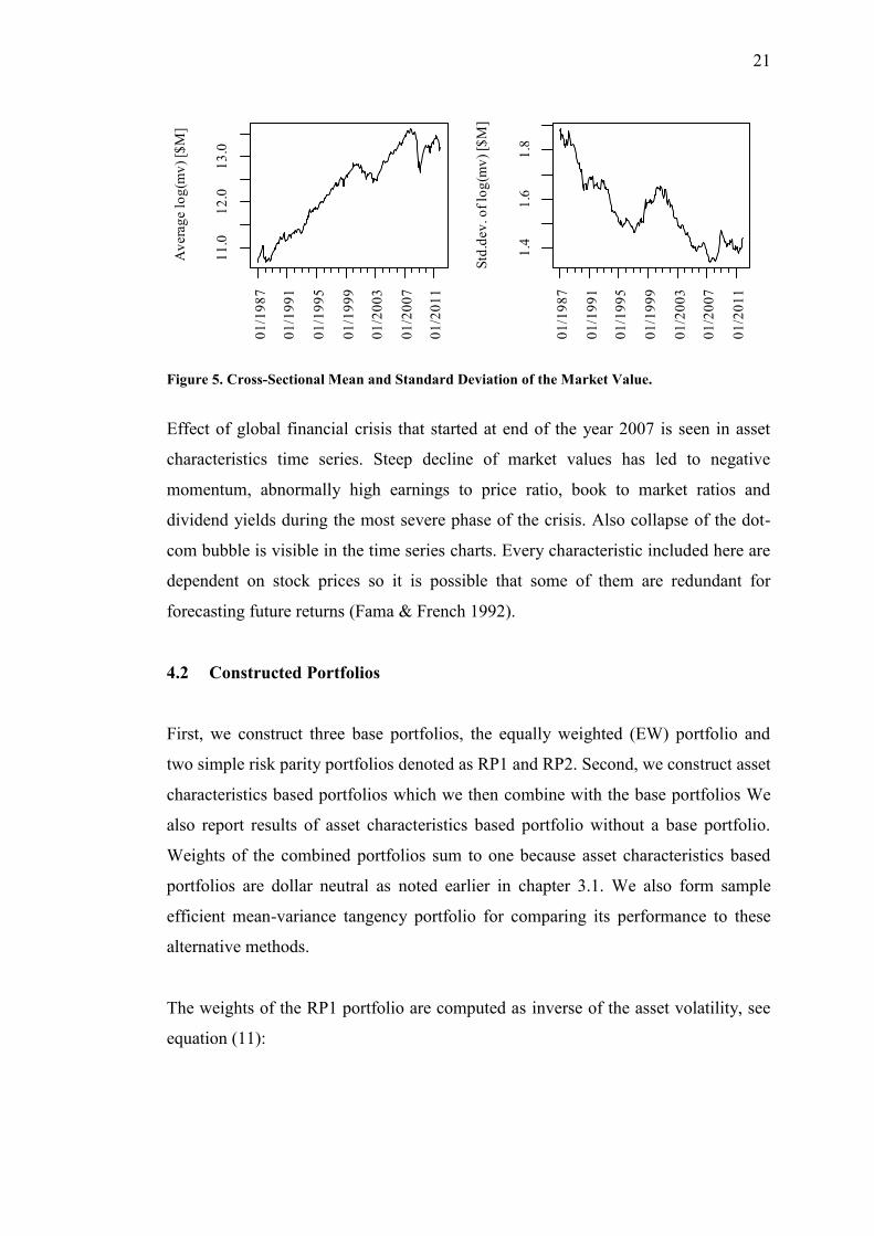
Figure 5. Cross-Sectional Mean and Standard Deviation of the Market Value. ................... 21
TABLES
Table 1. Summary statistics of total excess returns of country indices and the benchmark
index. ............................................................................................................................................ 18
Table 2. In-Sample Results and Performance Measures of Base Portfolios and the
Benchmark Index. ....................................................................................................................... 25
Table 3. Out-of-Sample Results and Performance Measures of Base Portfolios and the
Benchmark Index. ....................................................................................................................... 26
Table 4. In-Sample Statistics and Performance Measures of Asset Characteristics Based
Portfolio Without a Base Portfolio. ........................................................................................... 28
Table 5. Out-of-Sample Statistics and Performance Measures of Asset Characteristics Based
Portfolio Without a Base Portfolio. ........................................................................................... 29
Table 6. In-Sample and Out-of-Sample Estimates of the θ. .................................................... 31
Table 7. In-Sample Statistics and Performance Measures of Asset Characteristics Based
Portfolio Where the RP2 Portfolio is the Base Portfolio. ......................................................... 34
Table 8. Out-of-Sample Statistics and Performance Measures of Asset Characteristics Based
Portfolio Where the RP2 Portfolio is the Base Portfolio. ......................................................... 35
Table 9. In-Sample Statistics and Performance Measures of Asset Characteristics Based
Portfolios Where the Equally Weighted Portfolio is the Base Portfolio. ................................ 42
Table 10. Out-of-Sample Statistics and Performance Measures of Asset Characteristics
Based Portfolios Where the Equally Weighted Portfolio is the Base Portfolio. ..................... 43
Table 11. In-Sample Statistics and Performance Measures of Asset Characteristics Based
Portfolios Where the RP1 Portfolio is the Base Portfolio. ....................................................... 44
Table 12. Out-of-Sample Statistics and Performance Measures of Asset Characteristics
Based Portfolio Where the RP1 Portfolio is the Base Portfolio............................................... 45

5
1 INTRODUCTION
It is said that diversification is the only free lunch available in financial markets.
Portfolio optimization is all about diversification. Thus it is not surprising that
portfolio optimization is and has been interesting research topic for decades. Modern
portfolio theory had its start launch by Markowitz (1952) when he presented his
famous mean-variance model for portfolio optimization. The mean-variance model is
about finding portfolio weights that maximizes expected return with a given amount
of risk or alternatively minimizes risk with a given expected return level. Since then
many has contributed to this topic and theory has evolved greatly but still many
issues remain to be researched more closely. Portfolio optimization theory has direct
connection to real world finance and it surely is the motivation for many to search for
strategies that gain higher excess returns with less risk. Real world implementations
of modern portfolio optimization theory often face challenges and thus theories are
not very usable as is in practice. Theory itself may be very elegant and seem
righteous and sensible but when applied to real investment process many flaws may
be discovered. This applies also to the mean-variance model. Improvements to the
model to mitigate these common problems have been introduced in previous
literature.
This paper is about selecting country index portfolio using method introduced by
Brandt, Santa Clara and Valkanov (2007) and Hjalmarsson and Manchev (2009). In
their methods portfolio weights are directly estimated from asset characteristics.
Country indexes have similar characteristics and in this paper the following
characteristics are used in the method, price-to-earnings ratio, dividend yield, value,
size and momentum. MSCI World Index is used as benchmark when performance of
formed portfolios is analyzed. Portfolio performance metrics are measured by Sharpe
ratio, Jensen’s alpha and turnover.
The remainder of the paper is organized as follows. Section 2 is about literature
review of mean-variance portfolio solution, its common problems and presented
enhancements in earlier literature. Section 3 describes two alternative views for
portfolio optimization. First, portfolio solution based on asset characteristics is

6
presented and next, we take a look at a risk parity strategy. Section 4 is about data
used in the empirical part of the thesis. Also the characteristics included in the
parametric portfolio optimization model are described here. Section 5 presents the
results of the empirical research. Finally, section 6 concludes.

7
2 TRADITIONAL PORTFOLIO OPTIMIZATION
2.1 Mean-Variance Approach
Markowitz published mean-variance model for portfolio selection in his path-
breaking article in 1952 (Markowitz 1952). This model formed the foundation of the
so called Modern Portfolio Theory (MPT) and even after decades it is still inspiring
theoretical and empirical research today. Tobin’s well-known Two Fund Theorem
and the famous capital asset pricing model (CAPM) are great examples of
importance of Markowitz’s mean-variance model (Tobin 1958, Sharpe 1964, Lintner
1965a, Lintner 1965b).
Mean-variance model is concerned with investors acting under uncertainty.
Markowitz argues that investors are risk averse and only interested in myopically
optimizing variances and expected returns of their investment portfolios. The mean-
variance model aims to maximize expected return of the portfolio with a given
amount of risk or alternatively minimize the portfolio variance with a given expected
return target. This kind of optimization leads to efficient portfolios which form the
famous efficient frontier. Standard deviation of return is used as a proxy for risk and
asset returns are assumed to be jointly normally distributed. Other assumptions made
by the MPT includes that short selling is allowed, there is no transaction costs or
other constraints, asset positions are fully divisible and investor can lend and borrow
at risk free rate without restrictions. (Markowitz 1952, Sharpe 1964)
Intuition behind mean-variance model is that an asset weight in an investment
portfolio should not be selected independently from other assets. Rather, asset
weights should be obtained by statistical analysis where expected returns, variances
and covariance between assets are used as inputs. Markowitz suggests that portfolio
selection process may be divided into two stages. The first stage consists of creation
of beliefs about future performances of available securities. In the second stage these
newly formed beliefs are used for selecting weights for every asset in the portfolio.
Markowitz argues that if the future mean returns and covariance is known, the mean-
variance model results in the best possible portfolio solution in the risk-return sense.
Variance of a portfolio is lower than variance of any single asset when assets are not
8
perfectly positively correlated and short selling is allowed. Hence mean-variance
model illustrates the benefits of diversification and higher expected returns can only
be gained by taking more risk. (Markowitz 1952, Sharpe 1964)
2.2 Criticism of Mean-Variance Approach
There is no doubt of importance of the mean-variance model for the field of
quantitative portfolio optimization. Yet, mean-variance model has also received
notable amount of criticism. The mean-variance optimization requires investor to
estimate future expected mean returns, variances and covariance for all assets in the
asset universe but it does not take into account possible errors in these estimates
(Barry 1974). Instead, mean-variance optimization process considers given estimates
to be absolutely accurate. Using historical means and covariance as estimates for
mean-variance process is not optimal (Michaud 1989, Kan and Zhou 2007).
DeMiguel, Garlappi and Uppal (2009) show that out-of-sample performance of the
sample based mean-variance portfolio is not better than the performance of the equal
weighted portfolio. It is easy to argue that an investor can have proper views of
future performance only for a subset of assets at the most and even then these views
may be erroneous. This feature of the mean-variance model is called as estimation
error and it is the main problem in the model.
Best and Grauer (1991) show that even slight modifications to estimates of expected
returns or covariance may lead to dramatic changes in portfolio weights. Chopra and
Ziemba (1993) show that estimation errors in mean returns have stronger impact on
portfolio allocation than estimation errors in the covariance matrix. Michaud (1989)
call mean-variance optimizer as an error maximizer. He argues that mean-variance
optimizer puts too much weight on assets with large expected returns, small
variances and negative correlations and correspondingly mean-variance optimizer
underweight assets with low expected returns, high variances and positive
correlations. Michaud (1989) state also that these securities are most likely the ones
with large estimation errors.
In addition to estimation error, the mean-variance model has also been criticized for
its simplifying assumptions. Lintner (1969) and Merton (1973) list some of these
9
prerequisite assumptions: there are no taxes and transaction costs nor problems with
indivisibilities of assets; single trading period model, there is a riskless asset
available for every investor to hold or borrow at a fixed interest rate; all investors act
in terms of identical joint probability distributions; short selling is allowed and
possible for all; market is always in equilibrium. Many of these assumptions can be
rejected just by using common sense as they match poorly with the real world
financial markets.
Single investment period does not hold in real life where stocks are bought and sold
every bank day. This kind of assumption would lead to ignoring dynamic nature of
financial markets. Correlations between assets are not fixed and depend on
systematic relationships between the assets. When these relationships change
correlations change. For example correlations tend to increase during bear markets,
because all asset prices fall together (Campbell, Koedijk and Kofman 2002).
Taxes and transaction costs cannot be omitted in real life investments. Brennan
(1970) studies personal tax effects on corporation valuation. Levy (1978)
incorporates transaction costs in his study. In real world borrowing has also some
restrictions. Usually borrower needs to pledge some collateral to secure a loan. Thus
an investor has a limit in the amount she can borrow. Black (1972) has studied
setting in which there is no riskless asset. Short selling is not unlimitedly available
for every investor. Markowitz (1990) considers effects of short selling restrictions.
Assuming that market is always in equilibrium means that greater returns can only be
gained by taking more risk. However, in the modern financial literature there is
evidence of anomalies that have predictability of returns. Fama and French (1988)
show that dividend to price ratio can forecast future returns. This and few other
anomalies are discussed in more detail in chapter 4.
2.3 Extensions
The estimation error problem of the mean-variance model has motivated researchers
to find different improving methods to mitigate the problem. There exists vast

10
amount of literature presenting implementations like deploying portfolio constraints,
use of factor models and Bayesian shrinkage approach.
Frost and Savarino (1988), Chopra (1993) and Jagannathan and Ma (2003) propose
rules for constraining portfolio weights. Their studies show that imposing
shortselling constraints reduce the sensitivity of the portfolio composition to
estimation errors. Goldfarb and Iyengar (2003) and Garlappi, Uppal and Wang
(2007) deal with robust portfolio selection problems where they treat market
parameters as bounded random values. MacKinlay and Pastor (2000) propose
missing-factor model for more stable estimations.
Chan, Karceski and Lakonish (1999) focus on estimating the covariance matrix with
different factor models. Their study shows that factor models help to improve the
portfolio performance by lowering the portfolio volatility. Ledoit and Wolf (2004a,
2004b) shrink sample-based values of the covariance matrix towards more central
values. Their method increases performance of the managed portfolio.
Black and Litterman (1992) propose approach where investor’s subjective views are
combined with estimates from the CAPM. Their model has been named logically as
Black-Litterman model. Pástor (2000) and Pástor and Stambaugh (2000) propose
Bayesian method where shrinkage target depends on the investor’s belief in an asset
pricing model. Jobson, Korkie and Ratti (1979) and Jorion (1985, 1986) use Bayes-
Stein shrinkage estimation which shrinks the asset’s sample mean toward a common
mean. Jorion (1985, 1986) sets the common mean to be the mean of the minimum
variance portfolio.
Demiguel, Garlappi and Uppal (2007) compare out of sample performance of
sample-based mean-variance model and 13 different extensions of it to performance
of the naïve equal weighted portfolio. None of the models they evaluated consistently
outperformed the equal weighted rule in terms of Sharpe ratio, certainty-equivalent
return or turnover. Demiguel et al. (2007) show that poor performance of mean-
variance based portfolios is due to small estimation window. They argue that
estimation window should be at least “3000 months for a portfolio with only 25
assets, and more than 6000 months for a portfolio with 50 assets”.

11
Kan and Zhou (2007) show that optimally combining the risk-free asset, the sample
tangency portfolio and the sample minimum variance portfolio outperforms portfolio
that is only composed of the risk-free asset and the sample tangency portfolio. Tu
and Zhou (2008) takes this model a step further and argue that their portfolio strategy
consistently performs well with estimation window as small as 120 months.

12
3 ALTERNATIVE METHODS FOR PORTFOLIO OPTIMIZATION
3.1 Asset Characteristics Based Model
Mean-variance approach has its drawbacks as mentioned in the previous chapter.
Brandt, Santa-Clara and Valkanov (2009) suggested portfolio selection process
without modeling probability distributions of expected returns. Instead, in their
model portfolio weights are derived directly from asset specific characteristics.
Demiguel et al. (2007) wrote in their paper that this kind of approach “can represent
a promising direction to pursue”. Hjalmarsson and Manchev (2012) also focus on
direct estimation of portfolio weights. Brandt et al. (2009) work with investor’s
general utility functions whereas Hjalmarsson and Manchev use mean-variance
formulation in the portfolio weight estimator. For simplicity taxes and transaction
costs are omitted.
Below we take a closer look on the method for modeling portfolio weights directly
from asset characteristics. For standardizing asset characteristics we adopt the same
technique as in Brandt et al. (2009). For rest of the direct estimation procedure we
follow method presented by Hjalmarsson and Manchev (2012). And eventually, we
form final portfolio weights similarly as in Brandt et al. (2009).
First of all, asset characteristics are standardized to have zero mean and unit
standard deviation for every cross-section with the following equation,
)(
)(,
,
t
ttiti
X
XXx
, (1)
where xi,t is standardized characteristic for i:th asset at t:th time period, Xi,t represents
raw characteristic value, μ(Xt) is cross sectional mean of asset and σ(Xt)is cross
sectional standard deviation of asset characteristics on t:th time period. Alternatively
characteristics could be normalized to have values between -1 and 1 as in
Hjalmarsson and Manchev (2012). Standardization as in equation (1) ensures
characteristics to have zero mean. This is not the case with normalization. Depending

13
on the deviation of the characteristic the mean after normalization will likely be
different from zero.
Suppose investor’s problem is to maximize her portfolio return according to
following equation:
T
t
tttttw
rwrwT 1
21
'1
' ))(2
(1
max
, (2)
where w is an n x 1 vector of portfolio weights, rt+1 hold excess returns on assets
from period t to t+1 and γ is the coefficient of relative risk aversion (Hjalmarsson &
Manchev 2012). If we parameterize the portfolio weights, w, as a function of the
asset characteristics, x:
tt xw , (3)
and denote the sum of multiplication of asset specific characteristics by
corresponding excess return at each time period by
1'
1 ttt rxr , (4)
we get the following estimation problem,
T
t
tt rrT 1
21
'1
' ))(2
(1
max
, (5)
where θ is the estimates of characteristics loading on portfolio weights (Hjalmarsson
& Manchev 2012). The first order conditions for equation (5) are given by
T
t
ttt rrrT 1
11'
1 0))((1
, (6)
and finally θ can be estimated from

14
T
t
tt
T
t
t rT
rrT 1
1
1
'1
1
1
111~
(7)
(Hjalmarsson & Manchev 2012). Coefficients of θ are constant across assets and
through time (Brandt et al. 2009)
Hjalmarsson and Manchev propose that θ can be estimated also with ordinary least
square (OLS) regression as in Britten-Jones (1999). Britten-Jones shows that
regression of vector of ones onto a set of excess returns without an intercept term
results in the tangency portfolio weights when weights are scaled to sum to one.
Equations (8) and (9) capture this idea into the direct portfolio weight estimation
problem. The OLS regression equation is given by
ubrl , (8)
where l is vector of ones and b is the vector of regression coefficients and u is the
error term. Scaling coefficients b to sum to one results in the estimation of θ,
bl
b'
. (9)
After θ is estimated, the portfolio weights are given by the equation (3). These
weights form a dollar neutral long-short portfolio like Hjalmarsson & Manchev
(2012) apply in their paper. The dollar neutrality or other words weights summing to
zero is direct consequence of standardizing characters to have zeroed mean. Brandt et
al. propose that weights given by asset characteristics strategy can be thought as
deviation from a benchmark portfolio. Equation (10) describes this idea as follows:
ti
t
titi xN
ww ,'
,,
1 , (10)
15
where w is the weight vector of the base portfolio and Nt represents time varying
number of assets available for an investor. A base portfolio could be for example the
market portfolio or equal weighted portfolio.
3.2 Risk Parity
Risk parity strategies represent another approach that does not require estimates of
expected returns and has increased its popularity among researchers and practitioners
during the last ten years. The risk parity strategies focus on balancing amount of risk
per each asset in the portfolio – that is, diversifying by risk sources instead of by
dollars. Assets with low (high) risk are overweighted (underweighted) when
compared to market portfolio.
Allocation of 60 percent to stocks and 40 percent to bonds can be stated as normal
allocation of wealth. Total risk of the 60/40 stock/bond portfolio is dominated by
stock market risk because it is significantly more volatile than bond market. Chaves,
Hsu, Li and Shakernia (2011) show that risk parity strategy performs similarly
against 60/40 and equally weighted portfolios and clearly better than minimum-
variance or mean-variance portfolios in terms of Sharpe ratio. Although they note
that performances of different strategies vary greatly depending on the time period
and on the universe of asset classes included. (Chaves, Hsu, Li & Shakernia 2011)
In addition of allocation between different asset classes, risk parity strategy can be
applied in portfolio allocation within an asset class. Teiletche, Roncalli and Maillard
(2010) test equal risk contribution (ERC) strategy within two different set of asset
classes. The first set consists of ten industry sectors for the US equity market and the
second set is based on a basket of light agricultural commodities. They compare an
ERC portfolio with minimum variance and equally-weighted portfolios and note that
ERC portfolio is an attractive alternative to these. In volatility sense the ERC
portfolio lie between the two benchmark portfolios. With US equity market industry
sector data the risk adjusted performance of the ERC strategy is slightly better than
that of the equally weighted portfolio while minimum variance portfolio dominates
both of them due to its low volatility. When measured by the raw return levels, the
ERC strategy is on par with the equally weighted case and the minimum variance

16
portfolio receives the lowest return of the three portfolios. The ERC strategy
generates portfolios which may be concentrated in terms of weights but not nearly as
heavily as with minimum variance strategy. On the other hand, the ERC strategy is
diversified between risk sources while the equally weighted portfolio is more
concentrated in terms of risk sources. (Teiletche, Roncalli & Maillard 2010)
17
4 EMPIRICAL RESEARCH
4.1 Data and Characteristics
4.1.1 Overview
The data includes total return indexes for stock markets in 21 countries and the
following characteristics data sets for these markets: earnings to price ratio, dividend
yield, price to book ratio, market value. These data sets are obtained from Thomson
Reuters Datastream. As a risk-free rate we use U.S. dollar based 1-month London
interbank offered rate (LIBOR) and as a benchmark market return we use Morgan
Stanley Capital International gross return world index (MSCI WI). All the data are
U.S. dollar based and on monthly frequency from January of 1986 through
December of 2011. The first 12 months of the data are used only to create
momentum data. Table 1 lists the 21 country indices and the benchmark index
included in the study with summary statistics. The statistics show that different
markets are homogeneous with few exceptions. Markets of Austria and Hong Kong
have exceptionally high kurtosis.
4.1.2 Asset Characteristics
As already mentioned, we selected book to market ratio, market value, momentum,
dividend yield and earnings to price ratio to be the variables included in the asset
characteristics based model. There are two reasons why we ended up with these
specific characteristics. First, these characteristics have been commonly used in the
previous literature in the field of quantitative portfolio optimization. Second, our
study does not aim to find the optimal set of asset characteristics to be used with the
asset characteristics based model. Our goal is just to demonstrate the model with a
set of characteristics.
Earnings to price ratio (EP) or its inverse, price to earnings ratio (PE) is trivial and
widely used stock valuation measure. Portfolios with low PE ratios tend to earn
higher rates of return than portfolios with high PE ratios (Basu 1977). Basu (1983)
confirms this effect even after taking into account firm size. Ball (1978) argues that
18
EP can capture also other unknown risk factors. Dividend yield (DY) is another
important ratio in investing. It represents the amount of dividends firms pay relative
to their stock prices. Dividend yield has been reported to have predictability over
future returns (Fama & French 1988, Arnott & Asness 2003, Cochrane 2007).
Table 1. Summary statistics of total excess returns of country indices and the benchmark index.
Market Max Min Mean std kurt skew
Austria 16.43 -57.32 7.37 24.44 15.50 -2.27
Australia 19.93 -42.09 3.44 24.34 6.03 -1.16
Belgium 14.94 -39.20 4.42 20.18 7.78 -1.55
Canada 18.48 -30.95 6.37 19.82 5.09 -1.26
Denmark 18.36 -30.80 7.63 20.13 3.43 -0.85
Finland 25.77 -34.24 4.12 29.83 1.09 -0.25
France 17.56 -24.40 4.61 21.12 1.23 -0.63
Germany 17.56 -23.27 2.75 21.60 1.59 -0.75
Hong Kong 25.33 -61.16 7.10 28.75 10.75 -1.60
Ireland 18.01 -29.50 4.00 23.31 2.87 -0.97
Italy 18.89 -26.44 -1.24 23.97 0.59 -0.24
Japan 23.29 -19.98 -2.63 21.96 0.60 0.11
Malaysia 37.48 -40.88 6.16 29.90 4.82 -0.63
Netherlands 15.05 -37.14 4.50 20.46 6.81 -1.60
New Zealand 25.47 -20.72 4.16 22.26 1.13 -0.22
Norway 17.25 -36.72 8.76 27.45 3.70 -1.23
Singapore 22.98 -46.89 4.86 25.41 6.91 -1.32
Spain 19.30 -28.22 4.61 22.96 2.00 -0.73
Switzerland 14.00 -20.80 6.21 17.38 1.57 -0.73
UK 13.75 -24.52 5.22 18.13 2.48 -0.64
US 12.04 -23.91 4.99 16.15 3.17 -1.04
MSCI WI 10.69 -21.20 2.72 16.09 2.24 -0.87
This table shows the performance of the benchmark and country indices in the period of 01/1987 to 12/2011. First
column reports the market or country index and following six columns reports maximum, minimum, annualized
mean, annualized standard deviation, excess kurtosis and skewness of the monthly return series.
Banz (1981) showed that size factor, measured by market value (MV) of an asset,
has forecasting power on future returns. On average, firms with smaller market
capitalization tend to earn higher risk adjusted returns than those with bigger market
capitalizations (Banz 1981). For size factor in our study, we use log of market value.
Fama and French (1992) show with U.S. stocks that book to market ratio (B/E) is
more powerful return estimator than market value. Stocks with high book to market
19
ratios earn higher returns than growth stocks (Fama & French 1992). Value effect is
also observed in international returns (Fama & French 2012, Asness, Moskowitz &
Pedersen 2013). For value factor in our study, we use log book to market value.
There is also evidence of momentum (MOM) effect, Jegadeesh and Titman (1993)
report that a momentum strategy generates significant positive returns in the US
stock markets. Momentum effect in international returns is reported by Fama and
French (2012) and Asness et al. (2013). In our study, we calculate momentum as
cumulative log return from past twelve months as there is no evident of short term
reversal in country index returns (Patro and Wu 2004). Size, value and momentum
anomalies have been included in multifactor extensions of the CAPM. Fama and
French (1993) used size and value effects in their famous 3-factor model. Carhart
added one more factor, momentum, and formed a 4-factor model (Carhart 1997).
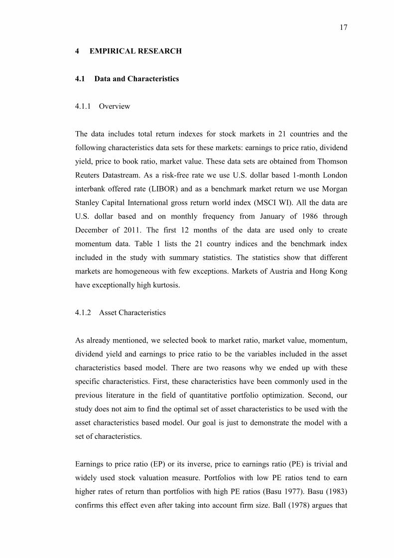
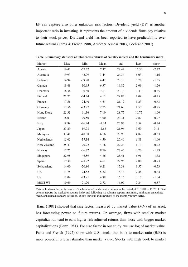
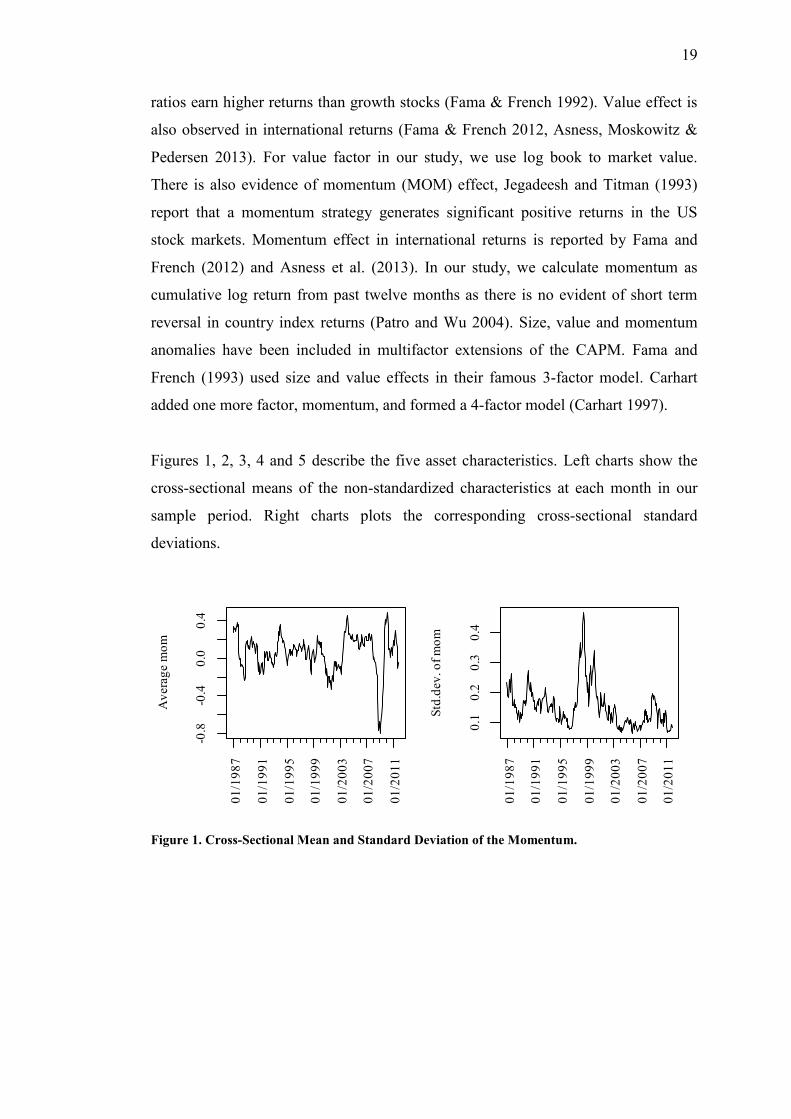
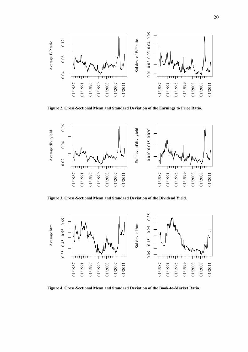
Figures 1, 2, 3, 4 and 5 describe the five asset characteristics. Left charts show the
cross-sectional means of the non-standardized characteristics at each month in our
sample period. Right charts plots the corresponding cross-sectional standard
deviations.
Figure 1. Cross-Sectional Mean and Standard Deviation of the Momentum.
-0.8
-0.4
0.0
0.4
01
/19
87
01
/19
91
01
/19
95
01
/19
99
01
/20
03
01
/20
07
01
/20
11
Av
era
ge m
om
0.1
0.2
0.3
0.4
01
/19
87
01
/19
91
01
/19
95
01
/19
99
01
/20
03
01
/20
07
01
/20
11
Std
.dev
. o
f m
om
20
Figure 2. Cross-Sectional Mean and Standard Deviation of the Earnings to Price Ratio.
Figure 3. Cross-Sectional Mean and Standard Deviation of the Dividend Yield.
Figure 4. Cross-Sectional Mean and Standard Deviation of the Book-to-Market Ratio.
0.0
40
.08
0.1
2
01
/19
87
01
/19
91
01
/19
95
01
/19
99
01
/20
03
01
/20
07
01
/20
11
Av
era
ge E
/P r
ati
o
0.0
10
.02
0.0
30
.04
0.0
5
01
/19
87
01
/19
91
01
/19
95
01
/19
99
01
/20
03
01
/20
07
01
/20
11
Std
.dev
. o
f E
/P r
ati
o
0.0
20
.04
0.0
6
01
/19
87
01
/19
91
01
/19
95
01
/19
99
01
/20
03
01
/20
07
01
/20
11
Av
era
ge d
iv. y
ield
0.0
10
0.0
15
0.0
20
01
/19
87
01
/19
91
01
/19
95
01
/19
99
01
/20
03
01
/20
07
01
/20
11
Std
.dev
. o
f d
iv. y
ield
0.3
50
.45
0.5
50
.65
01
/19
87
01
/19
91
01
/19
95
01
/19
99
01
/20
03
01
/20
07
01
/20
11
Av
era
ge b
tm
0.0
50
.15
0.2
50
.35
01
/19
87
01
/19
91
01
/19
95
01
/19
99
01
/20
03
01
/20
07
01
/20
11
Std
.dev
. o
f b
tm
21
Figure 5. Cross-Sectional Mean and Standard Deviation of the Market Value.
Effect of global financial crisis that started at end of the year 2007 is seen in asset
characteristics time series. Steep decline of market values has led to negative
momentum, abnormally high earnings to price ratio, book to market ratios and
dividend yields during the most severe phase of the crisis. Also collapse of the dot-
com bubble is visible in the time series charts. Every characteristic included here are
dependent on stock prices so it is possible that some of them are redundant for
forecasting future returns (Fama & French 1992).
4.2 Constructed Portfolios
First, we construct three base portfolios, the equally weighted (EW) portfolio and
two simple risk parity portfolios denoted as RP1 and RP2. Second, we construct asset
characteristics based portfolios which we then combine with the base portfolios We
also report results of asset characteristics based portfolio without a base portfolio.
Weights of the combined portfolios sum to one because asset characteristics based
portfolios are dollar neutral as noted earlier in chapter 3.1. We also form sample
efficient mean-variance tangency portfolio for comparing its performance to these
alternative methods.
The weights of the RP1 portfolio are computed as inverse of the asset volatility, see
equation (11):
11
.01
2.0
13
.0
01
/19
87
01
/19
91
01
/19
95
01
/19
99
01
/20
03
01
/20
07
01
/20
11
Av
era
ge l
og
(mv
) [$
M]
1.4
1.6
1.8
01
/19
87
01
/19
91
01
/19
95
01
/19
99
01
/20
03
01
/20
07
01
/20
11
Std
.dev
. o
f lo
g(m
v)
[$M
]
22
)(
1
,
,
ti
tir
w
, (11)
where σ(ri,t) is the volatility of an asset i at time period t, and then scaling the weights
to sum to one. Asness, Frazzini and Pedersen (2012) use similar method for risk
parity strategy. Note, that this kind of simple risk parity strategy omits the covariance
structure between the assets while formerly mentioned ERC strategy takes it in the
account.
The weights of the RP2 portfolio are computed as inverse of the asset variance, see
equation (12):
)(
1
,2,
ti
tir
w
, (12)
where σ2(ri,t) is the variance of an asset i at time period t, and again the final weights
are received by scaling them to sum to one. The difference between the RP1 and the
RP2 strategies is that RP2 overweight (underweight) low (high) volatile assets a bit
more than the RP1 strategy.
For asset characteristics based portfolios we form single-characteristic portfolios
with every characteristic and two combinations of characteristics: (i) book to market
ratio, market value and momentum and, (ii) all five characteristics. At first, the
characteristics are standardized with the equation (1) and then the estimates of
characteristics loading on portfolio weights, θ, is received with the equations (8) and
(9). Asset characteristics based portfolio weights are then computed with the
equation (3) and final portfolio weights, a combination of a base portfolio and an
asset characteristics based portfolio, is computed with the equation (10).
The results of all constructed portfolios are presented in chapter 5. In-sample results
are obtained using the data from the whole sample and out-of-sample results are
computed with all the data available at the time of portfolio formation from the
beginning of the full sample period. The first out-of-sample portfolio is formed with

23
the first 60 months of data. For portfolio performance measures we compute three
quantities; Sharpe ratio, Jensen’s alpha and turnover. These metrics are explained in
more detail in chapter 4.3 below. Our objective is to observe the importance of the
selected asset characteristics for portfolio performance and the performances of the
base portfolios, the asset characteristics based portfolios and the combinations of
them.
4.3 Performance Metrics
4.3.1 Sharpe Ratio
Sharpe ratio is very commonly used for portfolio performance measurements. It tells
portfolio’s return per one unit of risk, in other words, risk-adjusted return. It is
defined as portfolio return over risk-free rate divided by standard deviation of that
return. Equation (13) is mathematical form of the Sharpe ratio of portfolio k:
k
fk
k
rrSR
(13)
where rk is the return of portfolio k, rf is the risk-free rate and σk is standard deviation
of portfolio k. The higher the Sharpe ratio better is the performance of the portfolio.
In addition to bare Sharpe ratios we also compute difference of portfolio Sharpe
ratios compared to that of the benchmark.
4.3.2 Jensen’s Alpha
Jensen’s alpha is risk-adjusted performance measure which represents the average
portfolio return over the return predicted by the CAPM with given portfolio beta and
benchmark return. Equation (14) is the mathematical representation of it:
))(( fbkfkk rrrr , (14)

24
where αk is the alpha for the portfolio k, rk is the return of the portfolio, rf is the risk-
free rate, βk is the portfolio beta and rb is the return of the benchmark or market
portfolio. Positive and large alpha is desirable as it suggests about portfolio strategy
that is beating its benchmark portfolio.
4.3.3 Turnover
Turnover measure reports average percentage of wealth traded at each rebalancing
moment. We use the same method to compute the portfolio turnover as in DeMiguel
& al. (2007). As equation (15) shows, the portfolio turnover is defined as the average
sum of the trades across N available assets:
T
t
N
j
tjktjk wwT
Turnover1 1
,,1,, )ˆˆ(1
, (15)
where 1,,ˆ tjkw is the weight of portfolio k after rebalancing, tjkw ,,ˆ is the weight
before rebalancing and T represents number of trading periods. Although we do not
include effect of transaction costs in our study, portfolio turnover gives indirectly a
sense of magnitude of the proportional transaction costs for each portfolio.
25
5 RESULTS AND DISCUSSION
5.1 Preliminary Results
All the returns reported in this study are excess log returns and taxes and transaction
costs are omitted. The in-sample and out-of-sample results and performance
measures of base portfolios are shown in table 2 and 3. These tables contain also the
same statistics for the benchmark index, MSCI WI, and for the sample efficient
mean-variance tangency portfolio (MVTAN).
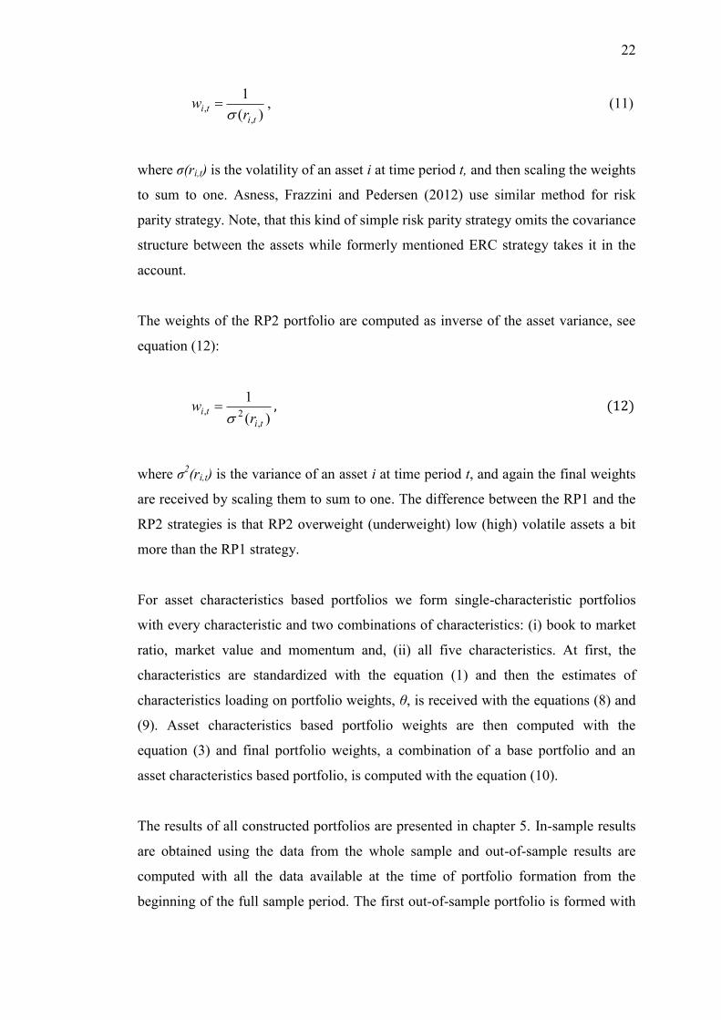
Table 2. In-Sample Results and Performance Measures of Base Portfolios and the Benchmark
Index.
Panel A: Summary statistics of the return series
Strategy Max Min Mean Std kurt skew min w max w
EW 12.66 -26.59 4.53 17.62 4.57 -1.33 4.76 4.76
RP1 12.41 -26.38 4.53 17.34 4.56 -1.33 3.54 6.55
RP2 12.17 -26.07 4.55 17.07 4.52 -1.33 2.56 8.78
MVTAN 32.66 -64.90 27.36 36.18 5.56 -0.97 -120.90 180.34
MSCI WI 10.69 -21.20 2.30 15.98 2.25 -0.91
Panel B: Performance measures
Strategy SR SR diff alpha beta turnover
EW 0.26 0.11 0.36 0.12 4.83
(1.28) (0.41) (1.21) (1.85)
RP1 0.26 0.12 0.35 0.12 4.71
(1.30) (0.42) (1.23) (1.89)
RP2 0.27 0.12 0.36 0.12 4.60
(1.33) (0.44) (1.25) (1.93)
MVTAN 0.76 0.61 2.24 0.21 51.30
(3.77) (2.08) (3.71) (1.64)
MSCI WI 0.14
(0.72)
Panel A shows the in-sample results of base portfolios and the benchmark index in the period of 01/1987 to
12/2011. First column reports the investment strategy and following six columns reports maximum, minimum,
annualized mean return, annualized standard deviation, excess kurtosis and skewness of the monthly in-sample
return series. The two remaining columns report minimum and maximum weights in the period. EW = equal
weight portfolio, MVTAN = mean-variance tangency portfolio, RP1 = risk-parity portfolio where weights are
relational to inverse of the standard deviation of the return and RP2 = risk-parity portfolio where weights are
relational to inverse of the variance of the return. Panel B shows the in-sample performance measures of formed
portfolios. First column reports the investment strategy. Second column reports the annualized in-sample Sharpe
ratio with t-statistic in the parenthesis below. Third column reports annualized differences of Sharpe ratios
between the benchmark (MSCI WI) and strategies. Next two columns report the CAPM monthly alpha and beta.
The last column reports the average monthly turnover. The bolded values are statistically significant at least at
90% confidence level.
26
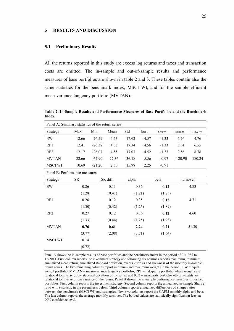
Table 3. Out-of-Sample Results and Performance Measures of Base Portfolios and the
Benchmark Index.
Panel A: Summary statistics of the return series
Strategy Max Min Mean Std kurt skew min w max w
EW 12.66 -26.59 4.50 17.59 3.80 -1.13 4.76 4.76
RP1 12.43 -26.74 4.53 17.40 4.05 -1.18 2.66 7.22
RP2 12.22 -26.79 4.59 17.23 4.23 -1.22 1.41 10.48
MVTAN 102.26 -271.36 0.28 80.95 76.33 -6.34 -3461.74 2592.14
MSCI WI 10.69 -21.20 2.76 15.52 2.18 -0.90
Panel B: Performance measures
Strategy SR SR diff alpha beta turnover
EW 0.26 0.08 0.34 0.17 4.76
(1.14) (0.26) (1.03) (2.32)
RP1 0.26 0.08 0.34 0.17 4.64
(1.16) (0.28) (1.05) (2.31)
RP2 0.27 0.09 0.34 0.16 4.55
(1.19) (0.30) (1.08) (2.31)
MVTAN 0.00 -0.17 -0.02 0.17 317.50
(0.02) (-0.55) (-0.01) (0.51)
MSCI WI 0.18
(0.79)
Panel A shows the out-of-sample results of base portfolios and the benchmark index in the period of 01/1992 to
12/2011. First column reports the investment strategy and following six columns reports maximum, minimum,
annualized mean return, annualized standard deviation, excess kurtosis and skewness of the monthly in-sample
return series. The two remaining columns report minimum and maximum weights in the period. EW = equal
weight portfolio, MVTAN = mean-variance tangency portfolio, RP1 = risk-parity portfolio where weights are
relational to inverse of the standard deviation of the return and RP2 = risk-parity portfolio where weights are
relational to inverse of the variance of the return. Panel B shows the out-of-sample performance measures of
formed portfolios. First column reports the investment strategy. Second column reports the annualized in-sample
Sharpe ratio with t-statistic in the parenthesis below. Third column reports annualized differences of Sharpe ratios
between the benchmark (MSCI WI) and strategies. Next two columns report the CAPM monthly alpha and beta.
The last column reports the average monthly turnover. The bolded values are statistically significant at least at
90% confidence level.
Performances of equally weighted, RP1 and RP2 portfolios are very close to each
other in both in-sample and out-of-sample. They show almost identical summary
statistics of the return series although there are considerable deviations in weights
between the portfolios as can be seen from the reported minimum and maximum
weights of the portfolios. All of the three portfolios gain better mean return than the
MSCI WI, the benchmark portfolio, but at the same time their standard deviations are
a bit higher too. Sharpe ratios of the three base portfolios are positive and better than
that of the benchmark portfolio but none of these Sharpe ratios are statistically
significant at the 90% confidence level. The same thing is seen in the evaluation of
27
the difference of the Sharpe ratios between each base portfolio and the benchmark
portfolio. The differences are positive but hypothesis of the null cannot be rejected at
the 90% confidence level in any case. All three base portfolio strategies generate
positive alphas but again, they are not statistically significant at the 90% confidence
level. Betas are low and statistically significant for all three base portfolios in both
in-sample and out-of-sample. The monthly mean turnover rates are reasonable for all
three portfolios; in average clearly less than 5% of wealth is traded at each
rebalancing moment.
The sample efficient mean-variance tangency portfolio shows measures which make
it stand out of the rest. In in-sample it dominates all other strategies by receiving
highest mean return and Sharpe ratio despite of receiving also the highest standard
deviation of return. The Sharpe ratio is statistically significant. The same applies also
to other in-sample performance measures of the MVTAN strategy. Sharpe ratio
difference to the benchmark portfolio is large and statistically significant even at the
95% confidence level. Also the alpha is large, over 2% and, statistically significant at
high confidence level. The minimum and maximum values of the weights give hint
of the unstable nature of the mean-variance strategy. The minimum and maximum
weights are large, representing values well over 100% short or long in one asset. In
out-of-sample the unstable nature of the mean-variance method is even more clearly
visible. Now the minimum and maximum weights show huge values, 3462% long
position in one asset or 2592% short position in one asset. Also the minimum and the
maximum values of the return series show large scale of deviation. When in the in-
sample the performance of the MVTAN was superior compared to other portfolios,
in the out-of-sample it performs the worst. The out-of-sample Sharpe ratio is zero,
difference of the Sharpe ration is negative as is the alpha. The turnover value of over
300% tells that MVTAN strategy requires heavy trading. An investor should trade
over three times of her own wealth in each rebalancing period in average. All in all,
the performance of the MVTAN is quite expected based on the chapter 2.2 and our
results support the idea that the equally weighted or even simple risk parity strategies
are great alternatives for the mean-variance approach.
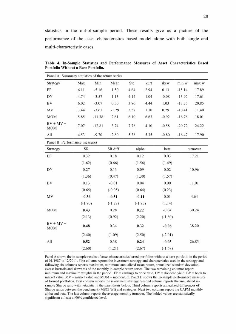
Table 4 represents in-sample results and performance measures of the asset
characteristic based portfolios without a base portfolio. Table 5 represents the same
28
statistics in the out-of-sample period. These results give us a picture of the
performance of the asset characteristics based model alone with both single and
multi-characteristic cases.
Table 4. In-Sample Statistics and Performance Measures of Asset Characteristics Based
Portfolio Without a Base Portfolio.
Panel A: Summary statistics of the return series
Strategy Max Min Mean Std kurt skew min w max w
EP 6.11 -5.16 1.50 4.64 2.94 0.13 -15.14 17.89
DY 4.74 -3.57 1.13 4.14 1.04 -0.08 -13.92 17.61
BV 6.02 -3.07 0.50 3.80 4.44 1.03 -13.75 20.85
MV 3.44 -3.61 -1.29 3.57 1.10 0.29 -10.41 11.40
MOM 5.85 -11.38 2.61 6.10 6.63 -0.92 -16.76 18.01
BV + MV +
MOM 7.07 -12.81 3.74 7.78 4.10 -0.58 -20.72 24.22
All 4.53 -9.70 2.80 5.38 5.35 -0.80 -16.47 17.90
Panel B: Performance measures
Strategy SR SR diff alpha beta turnover
EP 0.32 0.18 0.12 0.03 17.21
(1.62) (0.66) (1.56) (1.49)
DY 0.27 0.13 0.09 0.02 10.96
(1.36) (0.47) (1.30) (1.57)
BV 0.13 -0.01 0.04 0.00 11.01
(0.65) (-0.05) (0.64) (0.23)
MV -0.36 -0.51 -0.11 0.01 4.64
(-1.80) (-1.79) (-1.85) (1.14)
MOM 0.43 0.28 0.22 -0.04 30.24
(2.13) (0.92) (2.20) (-1.60)
BV + MV +
MOM 0.48 0.34 0.32 -0.06 38.20
(2.40) (1.09) (2.50) (-2.01)
All 0.52 0.38 0.24 -0.03 26.83
(2.60) (1.21) (2.67) (-1.68)
Panel A shows the in-sample results of asset characteristics based portfolios without a base portfolio in the period
of 01/1987 to 12/2011. First column reports the investment strategy and characteristics used in the strategy and
following six columns reports maximum, minimum, annualized mean return, annualized standard deviation,
excess kurtosis and skewness of the monthly in-sample return series. The two remaining columns report
minimum and maximum weights in the period. EP = earnings to price ratio, DY = dividend yield, BV = book to
market value, MV = market value and MOM = momentum. Panel B shows the in-sample performance measures
of formed portfolios. First column reports the investment strategy. Second column reports the annualized in-
sample Sharpe ratio with t-statistic in the parenthesis below. Third column reports annualized differences of
Sharpe ratios between the benchmark (MSCI WI) and strategies. Next two columns report the CAPM monthly
alpha and beta. The last column reports the average monthly turnover. The bolded values are statistically
significant at least at 90% confidence level.
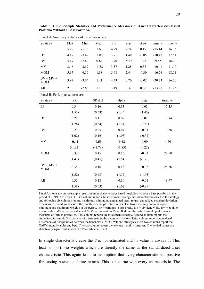
29
Table 5. Out-of-Sample Statistics and Performance Measures of Asset Characteristics Based
Portfolio Without a Base Portfolio.
Panel A: Summary statistics of the return series
Strategy Max Min Mean Std kurt skew min w max w
EP 5.98 -5.15 1.63 4.79 2.74 0.17 -15.14 16.83
DY 4.19 -3.42 1.06 3.71 1.40 -0.05 -10.48 17.61
BV 5.49 -2.62 0.84 3.70 5.39 1.27 -9.65 18.20
MV 3.46 -2.57 -1.38 3.37 1.28 0.57 -10.41 11.40
MOM 5.67 -6.59 1.88 5.68 2.44 -0.30 -16.76 18.01
BV + MV +
MOM 3.97 -3.65 1.41 4.33 0.70 -0.02 -20.23 16.70
All 2.70 -2.66 1.13 3.19 0.32 0.00 -13.91 11.23
Panel B: Performance measures
Strategy SR SR diff alpha beta turnover
EP 0.34 0.16 0.13 0.03 17.45
(1.52) (0.53) (1.45) (1.45)
DY 0.29 0.11 0.09 0.01 10.84
(1.28) (0.34) (1.24) (0.71)
BV 0.23 0.05 0.07 -0.01 10.88
(1.02) (0.16) (1.03) (-0.37)
MV -0.41 -0.59 -0.12 0.00 4.40
(-1.82) (-1.78) (-1.83) (0.22)
MOM 0.33 0.15 0.16 -0.03 29.58
(1.47) (0.45) (1.54) (-1.26)
BV + MV +
MOM 0.34 0.16 0.13 -0.02 24.26
(1.52) (0.48) (1.57) (-1.05)
All 0.35 0.18 0.10 -0.01 19.97
(1.58) (0.53) (1.62) (-0.87)
Panel A shows the out-of-sample results of asset characteristics based portfolios without a base portfolio in the
period of 01/1992 to 12/2011. First column reports the investment strategy and characteristics used in the strategy
and following six columns reports maximum, minimum, annualized mean return, annualized standard deviation,
excess kurtosis and skewness of the monthly in-sample return series. The two remaining columns report
minimum and maximum weights in the period. EP = earnings to price ratio, DY = dividend yield, BV = book to
market value, MV = market value and MOM = momentum. Panel B shows the out-of-sample performance
measures of formed portfolios. First column reports the investment strategy. Second column reports the
annualized in-sample Sharpe ratio with t-statistic in the parenthesis below. Third column reports annualized
differences of Sharpe ratios between the benchmark (MSCI WI) and strategies. Next two columns report the
CAPM monthly alpha and beta. The last column reports the average monthly turnover. The bolded values are
statistically significant at least at 90% confidence level.
In single characteristic case the θ is not estimated and its value is always 1. This
leads to portfolio weights which are directly the same as the standardized asset
characteristic. This again leads to assumption that every characteristic has positive
forecasting power on future returns. This is not true with every characteristic. The
30
size characteristic (MV) shows negative return in both in-sample and out-of-sample.
All the rest single characteristic portfolios generate positive returns in both sample
periods. The value effect (BV) shows the lowest positive return and momentum
effect (MOM) dominates the rest characteristics. These results are in-line with the
previous studies of the effects of these characteristics as discussed in the chapter
4.1.2.
In the in-sample, the negative Sharpe ratio, -0.36, of the MV portfolio is statistically
significant at 10% level and the positive Sharpe ratio, 0.43, of the MOM portfolio is
statistically significant even at 5% level. In out-of-sample, only the negative Sharpe
ratio of the MV portfolio is statistically significant at 10% level. The rest of the
Sharpe ratios of the single characteristic portfolios are not statistically significant at
10% level although EP portfolio shows promising values both in- and out-of-sample.
The difference of the Sharpe ratios between the single asset characteristics and the
benchmark portfolio are low and not statistically significant at 90% confidence level
except for the MV portfolio. The difference in the case of the MV portfolio is -0.51
in the in-sample and -0.59 in the out-of-sample. Both values are statistically
significant at 10% level.
All single characteristic portfolios show zero betas both in- and out-of-sample. The
portfolio performance evaluated by the monthly alphas highlight the same portfolios
as the Sharpe ratios. In in-sample, MV portfolio generates statistically significant
negative alpha and the monthly alpha of the MOM portfolio is positive and
statistically significant. In out-of-sample only the negative alpha of the MV portfolio
is statistically significant. Again, EP portfolio shows promising results also with the
alpha statistic although they are not statistically significant at 10% level. The
turnovers are similar in in-sample and out-of-sample periods. Magnitude of the
monthly average turnover of the EP portfolio shows that the strategy requires a lot of
trading. The same value of the MOM portfolio conveys that the momentum strategy
requires very heavy trading and thus its performance would be lower if the
transaction costs would be taken into account.
Tables 4 and 5 represent performance values and statistics also for the multi-
characteristic settings. We test multi-characteristic strategy with two different set of
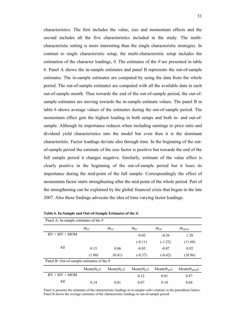
31
characteristics. The first includes the value, size and momentum effects and the
second includes all the five characteristics included in the study. The multi-
characteristic setting is more interesting than the single characteristic strategies. In
contrast to single characteristic setup, the multi-characteristic setup includes the
estimation of the character loadings, θ. The estimates of the θ are presented in table
6. Panel A shows the in-sample estimates and panel B represents the out-of-sample
estimates. The in-sample estimates are computed by using the data from the whole
period. The out-of-sample estimates are computed with all the available data in each
out-of-sample month. Thus towards the end of the out-of-sample period, the out-of-
sample estimates are moving towards the in-sample estimate values. The panel B in
table 6 shows average values of the estimates during the out-of-sample period. The
momentum effect gets the highest loading in both setups and both in- and out-of-
sample. Although its importance reduces when including earnings to price ratio and
dividend yield characteristics into the model but even then it is the dominant
characteristic. Factor loadings deviate also through time. In the beginning of the out-
of-sample period the estimate of the size factor is positive but towards the end of the
full sample period it changes negative. Similarly, estimate of the value effect is
clearly positive in the beginning of the out-of-sample period but it loses its
importance during the mid-point of the full sample. Correspondingly the effect of
momentum factor starts strengthening after the mid-point of the whole period. Part of
the strengthening can be explained by the global financial crisis that begun in the late
2007. Also these findings advocate the idea of time varying factor loadings.
Table 6. In-Sample and Out-of-Sample Estimates of the θ.
Panel A: In-sample estimates of the θ
ΘEP ΘDY ΘBV ΘMV ΘMOM
BV + MV + MOM -0.02 -0.26 1.28
(-0.11) (-1.22) (11.68)
All 0.15 0.06 -0.05 -0.07 0.92
(1.00) (0.41) (-0.37) (-0.42) (10.96)
Panel B: Out-of-sample estimates of the θ
Mean(ΘEP) Mean(ΘDY) Mean(ΘBV) Mean(ΘMV) Mean(ΘMOM)
BV + MV + MOM 0.12 0.01 0.87
All 0.14 0.01 0.07 0.10 0.68
Panel A presents the estimates of the characteristic loadings in in-sample with t-statistic in the parenthesis below.
Panel B shows the average estimates of the characteristic loadings in out-of-sample period.
32
Our estimates of the θ are similar with the estimates of the Hjalmarsson and
Manchev (2012). They include dividend yield, book to market ratio and momentum
characteristics in their work. They find momentum to be the most important
characteristic, just as we did. They report dividend yield to be not important
characteristic. This is the case also with our study. With book to market ratio our
estimates show clearly lower importance rate than estimates in Hjalmarsson and
Manchew (2012) does.
By comparing the results of the multi-characteristic portfolios to those of single
characteristic portfolios, we observe that multi-characteristic portfolios outperform
the single characteristic portfolios. Only MOM of the single characteristic portfolios
shows results close to the multi-characteristic strategies. This is not a surprise after
evaluation of estimates of the θ which showed large loading on the momentum
effect. The best results are obtained with the strategy which incorporates all five
asset characteristics. In in-sample the Sharpe ratios of the multi-characteristic
portfolios are statistically highly significant and better than any of the other
portfolios considered here. Also in the out-of-sample period the multi-characteristic
portfolios show the best Sharpe ratios although they are not statistically significant
anymore. The differences of the Sharpe ratios between the multi-characteristic
portfolios and the benchmark index are positive but the hypothesis of the null cannot
be rejected. The in-sample monthly mean alphas are positive and highly significant.
In out-of-sample, alphas appear to be a bit lower and not quite statistically significant
at the 10% level. The betas are slightly negative in both in- and out-of-sample but
only statistically significant in the in-sample. The monthly average turnovers are
quite high, around 20-25% of wealth traded in each rebalancing moment.
5.2 Results of Combined Portfolio
We choose RP2 to be the base portfolio for asset characteristics based portfolios
which we present here in the main part of the work because its performance metric
numbers show the best performance although the margin is almost indistinguishable
small, see tables 2 and 3. Results of asset characteristic based portfolios with EW and
RP1 portfolios as a base portfolio are presented in the appendix 1. Logically, asset
characteristic based portfolios with all three base portfolios show results close to
33
each other. This is because the performance of the base portfolios itself are close to
each other and asset characteristic based portfolios deviate the weights of the base
portfolios the same way.
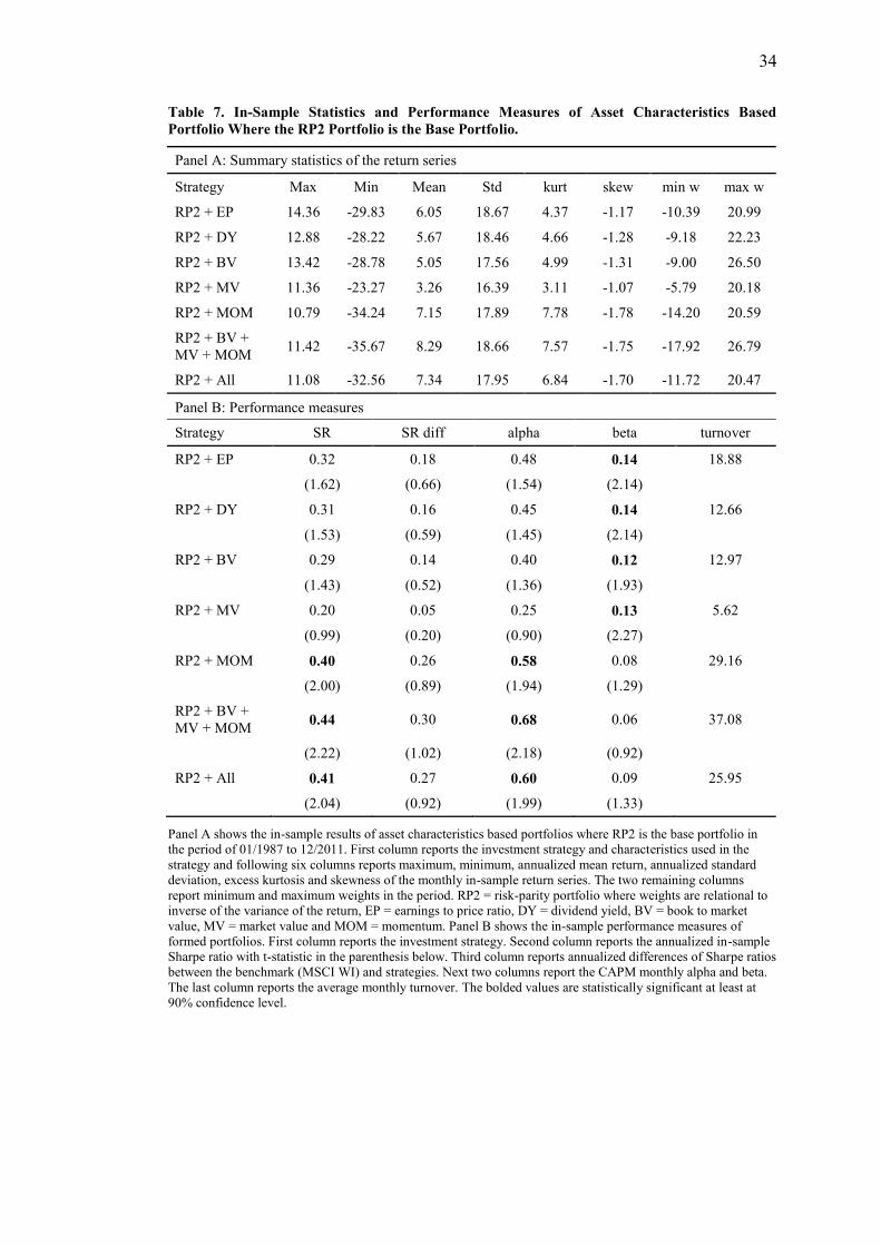
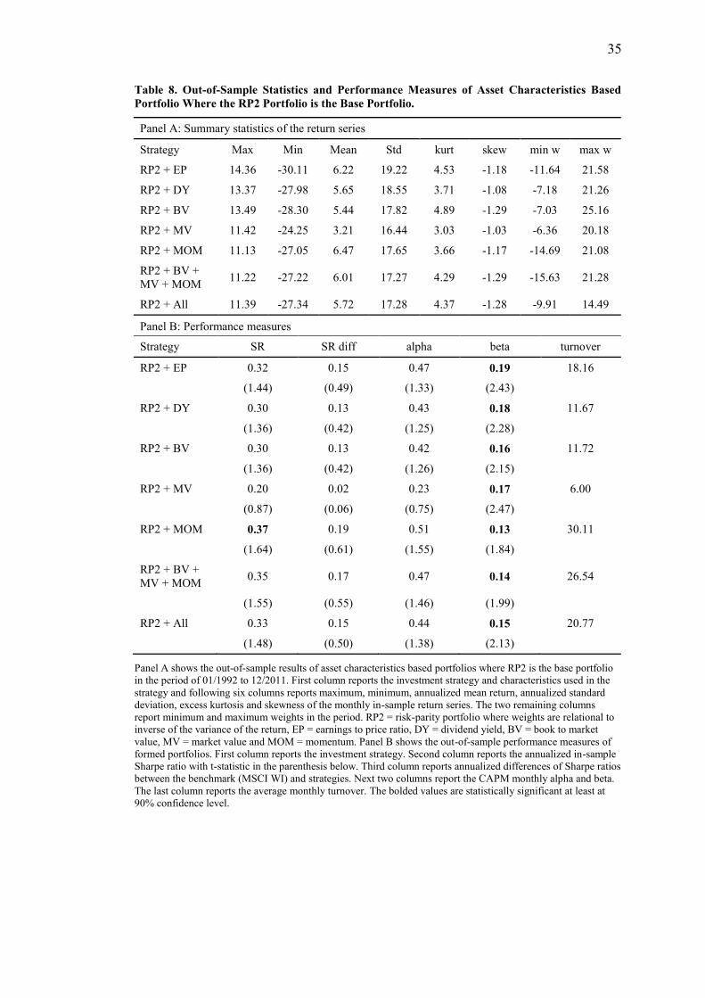
Table 7 and 8 show the in-sample and out-of-sample results and performance
measures of asset characteristic based portfolios combined with the RP2 portfolio.
As a common observation we state that combination of the base portfolio and the
asset characteristic based portfolios improve the results compared to those of
standalone portfolios. In the previous chapter we observed that in the asset
characteristic based portfolio setting the multi-characteristic strategies outperform
the single characteristic portfolios. Thus here we concentrate on the portfolios of RP2
portfolio combined with multi-asset characteristic strategies.
In-sample Sharpe ratios are close to each other showing 0.44 for the three
characteristics case and 0.39 with all five characteristics. Both ratios are statistically
significant. The out-of-sample Sharpe ratios are a bit lower and not statistically
significant. Sharpe ratio differences are not statistically significant nor in in-sample
or out-of-sample. By this it is not so clear if RP2 portfolio combined with multi-
characteristic strategy beats the benchmark index in risk-adjusted metrics. The in-
sample alphas, 0.68 and 0.60 with three characteristics and five characteristics
respectively, are high and statistically significant at 5% level for both RP2 multi-
characteristic portfolios. The out-of-sample alphas are lower and not anymore
statistically significant even at the 10 % level. Betas for these portfolios are low in-
and out-of-sample. Turnovers are similar as they were with standalone asset
characteristic based portfolios. Although the important out-of-sample performance
measures are not quite statistically significant at the 90% confidence level, the
combination of simple risk parity strategy and multi-characteristic based portfolio
strategy shows interesting and promising results. With these results we agree with
what Demiguel et al. (2007) state; asset characteristic based portfolio solution can
represent a promising direction to pursue.
34
Table 7. In-Sample Statistics and Performance Measures of Asset Characteristics Based
Portfolio Where the RP2 Portfolio is the Base Portfolio.
Panel A: Summary statistics of the return series
Strategy Max Min Mean Std kurt skew min w max w
RP2 + EP 14.36 -29.83 6.05 18.67 4.37 -1.17 -10.39 20.99
RP2 + DY 12.88 -28.22 5.67 18.46 4.66 -1.28 -9.18 22.23
RP2 + BV 13.42 -28.78 5.05 17.56 4.99 -1.31 -9.00 26.50
RP2 + MV 11.36 -23.27 3.26 16.39 3.11 -1.07 -5.79 20.18
RP2 + MOM 10.79 -34.24 7.15 17.89 7.78 -1.78 -14.20 20.59
RP2 + BV +
MV + MOM 11.42 -35.67 8.29 18.66 7.57 -1.75 -17.92 26.79
RP2 + All 11.08 -32.56 7.34 17.95 6.84 -1.70 -11.72 20.47
Panel B: Performance measures
Strategy SR SR diff alpha beta turnover
RP2 + EP 0.32 0.18 0.48 0.14 18.88
(1.62) (0.66) (1.54) (2.14)
RP2 + DY 0.31 0.16 0.45 0.14 12.66
(1.53) (0.59) (1.45) (2.14)
RP2 + BV 0.29 0.14 0.40 0.12 12.97
(1.43) (0.52) (1.36) (1.93)
RP2 + MV 0.20 0.05 0.25 0.13 5.62
(0.99) (0.20) (0.90) (2.27)
RP2 + MOM 0.40 0.26 0.58 0.08 29.16
(2.00) (0.89) (1.94) (1.29)
RP2 + BV +
MV + MOM 0.44 0.30 0.68 0.06 37.08
(2.22) (1.02) (2.18) (0.92)
RP2 + All 0.41 0.27 0.60 0.09 25.95
(2.04) (0.92) (1.99) (1.33)
Panel A shows the in-sample results of asset characteristics based portfolios where RP2 is the base portfolio in
the period of 01/1987 to 12/2011. First column reports the investment strategy and characteristics used in the
strategy and following six columns reports maximum, minimum, annualized mean return, annualized standard
deviation, excess kurtosis and skewness of the monthly in-sample return series. The two remaining columns
report minimum and maximum weights in the period. RP2 = risk-parity portfolio where weights are relational to
inverse of the variance of the return, EP = earnings to price ratio, DY = dividend yield, BV = book to market
value, MV = market value and MOM = momentum. Panel B shows the in-sample performance measures of
formed portfolios. First column reports the investment strategy. Second column reports the annualized in-sample
Sharpe ratio with t-statistic in the parenthesis below. Third column reports annualized differences of Sharpe ratios
between the benchmark (MSCI WI) and strategies. Next two columns report the CAPM monthly alpha and beta.
The last column reports the average monthly turnover. The bolded values are statistically significant at least at
90% confidence level.
35
Table 8. Out-of-Sample Statistics and Performance Measures of Asset Characteristics Based
Portfolio Where the RP2 Portfolio is the Base Portfolio.
Panel A: Summary statistics of the return series
Strategy Max Min Mean Std kurt skew min w max w
RP2 + EP 14.36 -30.11 6.22 19.22 4.53 -1.18 -11.64 21.58
RP2 + DY 13.37 -27.98 5.65 18.55 3.71 -1.08 -7.18 21.26
RP2 + BV 13.49 -28.30 5.44 17.82 4.89 -1.29 -7.03 25.16
RP2 + MV 11.42 -24.25 3.21 16.44 3.03 -1.03 -6.36 20.18
RP2 + MOM 11.13 -27.05 6.47 17.65 3.66 -1.17 -14.69 21.08
RP2 + BV +
MV + MOM 11.22 -27.22 6.01 17.27 4.29 -1.29 -15.63 21.28
RP2 + All 11.39 -27.34 5.72 17.28 4.37 -1.28 -9.91 14.49
Panel B: Performance measures
Strategy SR SR diff alpha beta turnover
RP2 + EP 0.32 0.15 0.47 0.19 18.16
(1.44) (0.49) (1.33) (2.43)
RP2 + DY 0.30 0.13 0.43 0.18 11.67
(1.36) (0.42) (1.25) (2.28)
RP2 + BV 0.30 0.13 0.42 0.16 11.72
(1.36) (0.42) (1.26) (2.15)
RP2 + MV 0.20 0.02 0.23 0.17 6.00
(0.87) (0.06) (0.75) (2.47)
RP2 + MOM 0.37 0.19 0.51 0.13 30.11
(1.64) (0.61) (1.55) (1.84)
RP2 + BV +
MV + MOM 0.35 0.17 0.47 0.14 26.54
(1.55) (0.55) (1.46) (1.99)
RP2 + All 0.33 0.15 0.44 0.15 20.77
(1.48) (0.50) (1.38) (2.13)
Panel A shows the out-of-sample results of asset characteristics based portfolios where RP2 is the base portfolio
in the period of 01/1992 to 12/2011. First column reports the investment strategy and characteristics used in the
strategy and following six columns reports maximum, minimum, annualized mean return, annualized standard
deviation, excess kurtosis and skewness of the monthly in-sample return series. The two remaining columns
report minimum and maximum weights in the period. RP2 = risk-parity portfolio where weights are relational to
inverse of the variance of the return, EP = earnings to price ratio, DY = dividend yield, BV = book to market
value, MV = market value and MOM = momentum. Panel B shows the out-of-sample performance measures of
formed portfolios. First column reports the investment strategy. Second column reports the annualized in-sample
Sharpe ratio with t-statistic in the parenthesis below. Third column reports annualized differences of Sharpe ratios
between the benchmark (MSCI WI) and strategies. Next two columns report the CAPM monthly alpha and beta.
The last column reports the average monthly turnover. The bolded values are statistically significant at least at
90% confidence level.
36
6 CONCLUSIONS
Mean-variance model of Markowitz is important milestone in the quantitative
finance history but the model is problematic in the real portfolio optimization
implementations. The estimation error remains an insuperable problem to overcome
despite many of the presented improvements enhance the performance of the mean-
variance model.
We derive an asset characteristic based portfolio solution based on the work of
Brandt et al. (2009) and Hjalmarsson and Manchev (2012). Our objective is to show
the performance of this kind of simple portfolio optimization method with a set of
asset characteristics. We do not seek the best set of characteristics but choose five
characteristics that are common and are studied extensively in the earlier literature.
In addition to asset characteristic portfolios we show performances of equally
weighted portfolio and two simple risk parity strategies which we then combine with
the asset characteristic portfolio. We also show the importance of the selected asset
characteristics for portfolio performance. None of these alternative methods for
portfolio selection require the estimation of the future expected mean returns.
The data includes stock markets in 21 countries in the period of January 1986 to
December 2011. The data period can be described as challenging as it encloses many
bear and bull market sub-periods. The global financial crisis that begun in the late
2007 and recovery from it can be mentioned as the latest example. The asset specific
characteristics chosen are earnings-to-price ratio, dividend yield, price-to-book ratio,
market value and momentum.
Our results support the claim that equally weighted and simple risk parity portfolios
are great alternatives to mean-variance model. By out-of-sample performance
measures they beat the sample efficient mean-variance tangency portfolio easily.
They also show better performance values than the benchmark index, MSCI WI,
when measured by Sharpe ratio or Jensen’s alpha although we do not find these
measures to be statistically significant. Moreover, our results suggest that
performances of these alternative methods can be improved even further by
combining them with an asset characteristic based portfolio. The presented portfolio

37
selection methods provide stable and financially sensible results which are in-line
with the previous literature.
It is always important to consider the possibilities for real world implementations of
the portfolio strategies studied. The asset characteristic based portfolio of country
indices with or without a base portfolio weights could be implemented with country
index futures. Implementation with index following funds may be challenging
because of the negative weights the strategy may generate.
For future studies with the asset characteristic based portfolio selection with country
indices we raise two ideas. One, the model could be tested with other or additional
characteristics like difference of short and long interest rates or long-term return
reversal. Two, monthly time series of asset characteristics could be filtered simply by
moving average. Our undocumented quick tests imply that applying this would result
in lower turnover rates and improved performance measures across-the-board.
38
REFERENCES
Arnott, R. D. & Asness, C. S. (2003). Surprise! higher dividends= higher earnings
growth. Financial Analysts Journal 70-87.
Asness, C., Frazzini, A. & Pedersen, L. H. (2012). Leverage aversion and risk parity.
Financial Analysts Journal 68(1), 47-59.
Asness, C. S., Moskowitz, T. J. & Pedersen, L. H. (2013). Value and momentum
everywhere. The Journal of Finance 68(3), 929-985.
Ball, R. (1978). Anomalies in relationships between securities' yields and yield-
surrogates. Journal of Financial Economics 6(2), 103-126.
Banz, R. W. (1981). The relationship between return and market value of common
stocks. Journal of Financial Economics 9(1), 3-18.
Barry, C. B. (1974). Portfolio analysis under uncertain means, variances, and
covariances. The Journal of Finance 29(2), 515-522.
Basu, S. (1977). Investment performance of common stocks in relation to their
price‐earnings ratios: A test of the efficient market hypothesis. The Journal of
Finance 32(3), 663-682.
Basu, S. (1983). The relationship between earnings' yield, market value and return
for NYSE common stocks: Further evidence. Journal of Financial Economics
12(1), 129-156.
Best, M. J. & Grauer, R. R. (1991). On the sensitivity of mean-variance-efficient
portfolios to changes in asset means: Some analytical and computational results.
Review of Financial Studies 4(2), 315-342.
Black, F. (1972). Capital market equilibrium with restricted borrowing. Journal of
business 444-455.
Black, F. & Litterman, R. (1992). Global portfolio optimization. Financial Analysts
Journal 28-43.
Brandt, M. W., Santa-Clara, P. & Valkanov, R. (2009). Parametric portfolio policies:
Exploiting characteristics in the cross-section of equity returns. Review of
Financial Studies 22(9), 3411-3447.
Brennan, M. J. (1970). Taxes, market valuation and corporate financial policy.
National Tax Journal 417-427.
Campbell, R., Koedijk, K. & Kofman, P. (2002). Increased correlation in bear
markets. Financial Analysts Journal 87-94.

39
Carhart, M. M. (1997). On persistence in mutual fund performance. The Journal of
finance 52(1), 57-82.
Chan, L. K., Karceski, J. & Lakonishok, J. (1999). On portfolio optimization:
Forecasting covariances and choosing the risk model. Review of Financial
Studies 12(5), 937-974.
Chaves, D., Hsu, J., Li, F. & Shakernia, O. (2011). Risk parity portfolio vs. other
asset allocation heuristic portfolios. The Journal of Investing 20(1), 108-118.
Chopra, V. K. & Ziemba, W. T. (1993). The effect of errors in means, variances, and
covariances on optimal portfolio choice. The journal of portfolio management
19(2), 6-11.
Cochrane, J. H. (2008). The dog that did not bark: A defense of return predictability.
Review of Financial Studies 21(4), 1533-1575.
DeMiguel, V., Garlappi, L. & Uppal, R. (2009). Optimal versus naive diversification:
How inefficient is the 1/N portfolio strategy? Review of Financial Studies 22(5),
1915-1953.
Fama, E. F. & French, K. R. (1988). Dividend yields and expected stock returns.
Journal of Financial Economics 22(1), 3-25.
Fama, E. F. & French, K. R. (1992). The cross‐section of expected stock returns. the
Journal of Finance 47(2), 427-465.
Fama, E. F. & French, K. R. (1993). Common risk factors in the returns on stocks
and bonds. Journal of Financial Economics 33(1), 3-56.
Fama, E. F. & French, K. R. (2012). Size, value, and momentum in international
stock returns. Journal of Financial Economics 105(3), 457-472.
Frost, P. A. & Savarino, J. E. (1988). For better performance: Constrain portfolio
weights. The Journal of Portfolio Management 15(1), 29-34.
Garlappi, L., Uppal, R. & Wang, T. (2007). Portfolio selection with parameter and
model uncertainty: A multi-prior approach. Review of Financial Studies 20(1),
41-81.
Goldfarb, D. & Iyengar, G. (2003). Robust portfolio selection problems.
Mathematics of Operations Research 28(1), 1-38.
Hjalmarsson, E. & Manchev, P. (2012). Characteristic-based mean-variance portfolio
choice. Journal of Banking & Finance 36(5), 1392-1401.
Jagannathan, R. & Ma, T. (2003). Risk reduction in large portfolios: Why imposing
the wrong constraints helps. The Journal of Finance 58(4), 1651-1684.
40
Jegadeesh, N. & Titman, S. (1993). Returns to buying winners and selling losers:
Implications for stock market efficiency. The Journal of Finance 48(1), 65-91.
Jobson, J., Korkie, B., & Ratti, V. (1979). Improved estimation for markowitz
portfolios using james-stein type estimators. Proceedings of the American
Statistical Association, Business and Economics Statistics Section, , 41 279-284.
Jorion, P. (1985). International portfolio diversification with estimation risk. The
Journal of Business 58(3), 259-278.
Jorion, P. (1986). Bayes-stein estimation for portfolio analysis. Journal of Financial
and Quantitative Analysis 21(03), 279-292.
Kan, R. & Zhou, G. (2007). Optimal portfolio choice with parameter uncertainty.
Journal of Financial and Quantitative Analysis 42(03), 621-656.
Ledoit, O. & Wolf, M. (2004). Honey, I shrunk the sample covariance matrix. The
Journal of Portfolio Management 30(4), 110-119.
Ledoit, O. & Wolf, M. (2004). A well-conditioned estimator for large-dimensional
covariance matrices. Journal of multivariate analysis 88(2), 365-411.
Levy, H. (1978). Equilibrium in an imperfect market: A constraint on the number of
securities in the portfolio. The American Economic Review 643-658.
Lintner, J. (1965). Security prices, risk, and maximal gains from diversification*. The
Journal of Finance 20(4), 587-615.
Lintner, J. (1965). The valuation of risk assets and the selection of risky investments
in stock portfolios and capital budgets. The review of economics and statistics
13-37.
Lintner, J. (1969). The aggregation of investor's diverse judgments and preferences
in purely competitive security markets. Journal of Financial and Quantitative
Analysis 4(04), 347-400.
MacKinlay, A. C. & Pastor, L. (2000). Asset pricing models: Implications for
expected returns and portfolio selection. Review of Financial Studies 13(4), 883-
916.
Markowitz, H. (1952). Portfolio selection*. The journal of finance 7(1), 77-91.
Markowitz, H. M. (1990). Risk adjustment. Journal of Accounting, Auditing &
Finance 5(2), 213-225.
Merton, R. C. (1973). An intertemporal capital asset pricing model. Econometrica:
Journal of the Econometric Society 867-887.
Michaud, R. O. (1989). The markowitz optimization enigma: Is' optimized'optimal?
Financial Analysts Journal 31-42.

41
Pástor, Ľ. (2000). Portfolio selection and asset pricing models. The Journal of
Finance 55(1), 179-223.
Pástor, Ľ. & Stambaugh, R. F. (2000). Comparing asset pricing models: An
investment perspective. Journal of Financial Economics 56(3), 335-381.
Patro, D. K. & Wu, Y. (2004). Predictability of short-horizon returns in international
equity markets. Journal of Empirical Finance 11(4), 553-584.
Sharpe, W. F. (1964). Capital asset prices: A theory of market equilibrium under
conditions of risk*. The journal of finance 19(3), 425-442.
Teiletche, J., Roncalli, T. & Maillard, S. (2010). The properties of equally-weighted
risk contributions portfolios.
Tobin, J. (1958). Liquidity preference as behavior towards risk. The review of
economic studies 65-86.
Tu, J., & Zhou, G. (2008). Being naive about naive diversification: Can investment
theory be consistently useful? EFA 2008 Athens Meetings Paper,
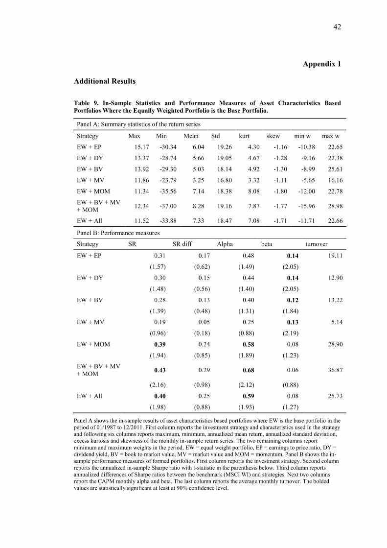
42
Appendix 1
Additional Results
Table 9. In-Sample Statistics and Performance Measures of Asset Characteristics Based
Portfolios Where the Equally Weighted Portfolio is the Base Portfolio.
Panel A: Summary statistics of the return series
Strategy Max Min Mean Std kurt skew min w max w
EW + EP 15.17 -30.34 6.04 19.26 4.30 -1.16 -10.38 22.65
EW + DY 13.37 -28.74 5.66 19.05 4.67 -1.28 -9.16 22.38
EW + BV 13.92 -29.30 5.03 18.14 4.92 -1.30 -8.99 25.61
EW + MV 11.86 -23.79 3.25 16.80 3.32 -1.11 -5.65 16.16
EW + MOM 11.34 -35.56 7.14 18.38 8.08 -1.80 -12.00 22.78
EW + BV + MV
+ MOM 12.34 -37.00 8.28 19.16 7.87 -1.77 -15.96 28.98
EW + All 11.52 -33.88 7.33 18.47 7.08 -1.71 -11.71 22.66
Panel B: Performance measures
Strategy SR SR diff Alpha beta turnover
EW + EP 0.31 0.17 0.48 0.14 19.11
(1.57) (0.62) (1.49) (2.05)
EW + DY 0.30 0.15 0.44 0.14 12.90
(1.48) (0.56) (1.40) (2.05)
EW + BV 0.28 0.13 0.40 0.12 13.22
(1.39) (0.48) (1.31) (1.84)
EW + MV 0.19 0.05 0.25 0.13 5.14
(0.96) (0.18) (0.88) (2.19)
EW + MOM 0.39 0.24 0.58 0.08 28.90
(1.94) (0.85) (1.89) (1.23)
EW + BV + MV
+ MOM 0.43 0.29 0.68 0.06 36.87
(2.16) (0.98) (2.12) (0.88)
EW + All 0.40 0.25 0.59 0.08 25.73
(1.98) (0.88) (1.93) (1.27)
Panel A shows the in-sample results of asset characteristics based portfolios where EW is the base portfolio in the
period of 01/1987 to 12/2011. First column reports the investment strategy and characteristics used in the strategy
and following six columns reports maximum, minimum, annualized mean return, annualized standard deviation,
excess kurtosis and skewness of the monthly in-sample return series. The two remaining columns report
minimum and maximum weights in the period. EW = equal weight portfolio, EP = earnings to price ratio, DY =
dividend yield, BV = book to market value, MV = market value and MOM = momentum. Panel B shows the in-
sample performance measures of formed portfolios. First column reports the investment strategy. Second column
reports the annualized in-sample Sharpe ratio with t-statistic in the parenthesis below. Third column reports
annualized differences of Sharpe ratios between the benchmark (MSCI WI) and strategies. Next two columns
report the CAPM monthly alpha and beta. The last column reports the average monthly turnover. The bolded
values are statistically significant at least at 90% confidence level.
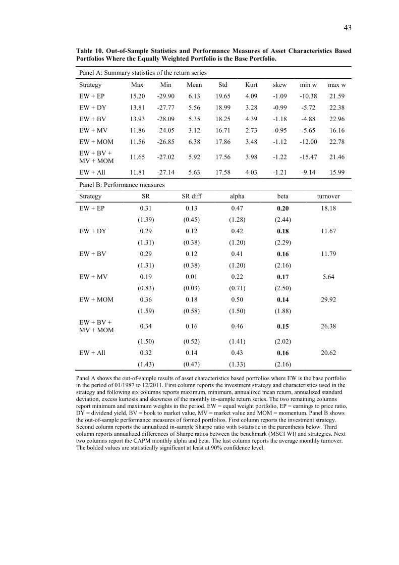
43
Table 10. Out-of-Sample Statistics and Performance Measures of Asset Characteristics Based
Portfolios Where the Equally Weighted Portfolio is the Base Portfolio.
Panel A: Summary statistics of the return series
Strategy Max Min Mean Std Kurt skew min w max w
EW + EP 15.20 -29.90 6.13 19.65 4.09 -1.09 -10.38 21.59
EW + DY 13.81 -27.77 5.56 18.99 3.28 -0.99 -5.72 22.38
EW + BV 13.93 -28.09 5.35 18.25 4.39 -1.18 -4.88 22.96
EW + MV 11.86 -24.05 3.12 16.71 2.73 -0.95 -5.65 16.16
EW + MOM 11.56 -26.85 6.38 17.86 3.48 -1.12 -12.00 22.78
EW + BV +
MV + MOM 11.65 -27.02 5.92 17.56 3.98 -1.22 -15.47 21.46
EW + All 11.81 -27.14 5.63 17.58 4.03 -1.21 -9.14 15.99
Panel B: Performance measures
Strategy SR SR diff alpha beta turnover
EW + EP 0.31 0.13 0.47 0.20 18.18
(1.39) (0.45) (1.28) (2.44)
EW + DY 0.29 0.12 0.42 0.18 11.67
(1.31) (0.38) (1.20) (2.29)
EW + BV 0.29 0.12 0.41 0.16 11.79
(1.31) (0.38) (1.20) (2.16)
EW + MV 0.19 0.01 0.22 0.17 5.64
(0.83) (0.03) (0.71) (2.50)
EW + MOM 0.36 0.18 0.50 0.14 29.92
(1.59) (0.58) (1.50) (1.88)
EW + BV +
MV + MOM 0.34 0.16 0.46 0.15 26.38
(1.50) (0.52) (1.41) (2.02)
EW + All 0.32 0.14 0.43 0.16 20.62
(1.43) (0.47) (1.33) (2.16)
Panel A shows the out-of-sample results of asset characteristics based portfolios where EW is the base portfolio
in the period of 01/1987 to 12/2011. First column reports the investment strategy and characteristics used in the
strategy and following six columns reports maximum, minimum, annualized mean return, annualized standard
deviation, excess kurtosis and skewness of the monthly in-sample return series. The two remaining columns
report minimum and maximum weights in the period. EW = equal weight portfolio, EP = earnings to price ratio,
DY = dividend yield, BV = book to market value, MV = market value and MOM = momentum. Panel B shows
the out-of-sample performance measures of formed portfolios. First column reports the investment strategy.
Second column reports the annualized in-sample Sharpe ratio with t-statistic in the parenthesis below. Third
column reports annualized differences of Sharpe ratios between the benchmark (MSCI WI) and strategies. Next
two columns report the CAPM monthly alpha and beta. The last column reports the average monthly turnover.
The bolded values are statistically significant at least at 90% confidence level.
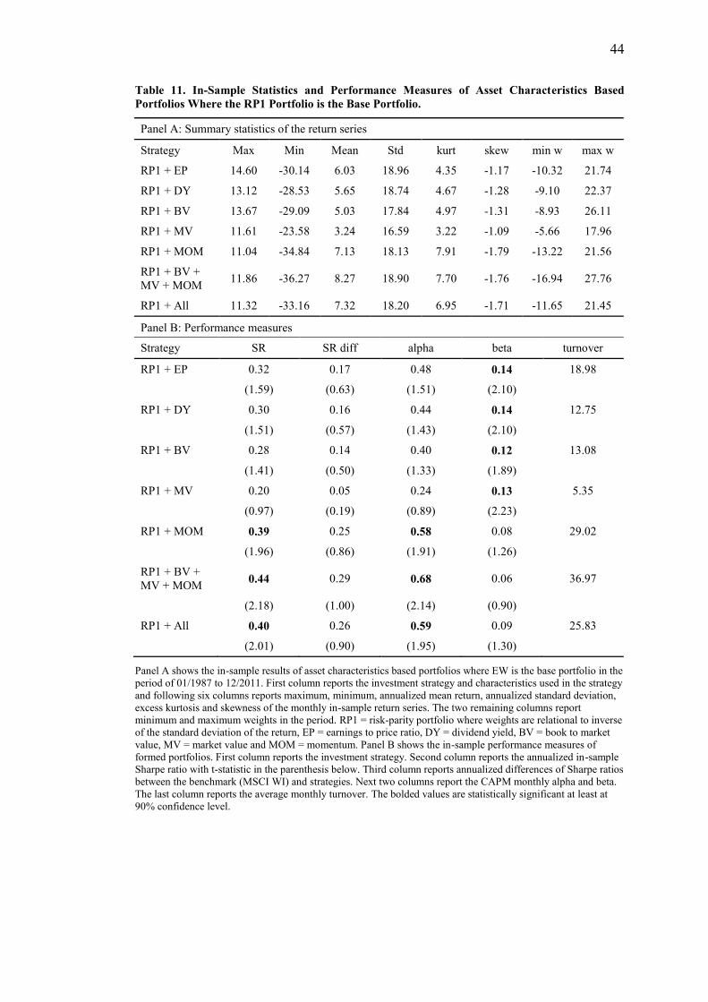
44
Table 11. In-Sample Statistics and Performance Measures of Asset Characteristics Based
Portfolios Where the RP1 Portfolio is the Base Portfolio.
Panel A: Summary statistics of the return series
Strategy Max Min Mean Std kurt skew min w max w
RP1 + EP 14.60 -30.14 6.03 18.96 4.35 -1.17 -10.32 21.74
RP1 + DY 13.12 -28.53 5.65 18.74 4.67 -1.28 -9.10 22.37
RP1 + BV 13.67 -29.09 5.03 17.84 4.97 -1.31 -8.93 26.11
RP1 + MV 11.61 -23.58 3.24 16.59 3.22 -1.09 -5.66 17.96
RP1 + MOM 11.04 -34.84 7.13 18.13 7.91 -1.79 -13.22 21.56
RP1 + BV +
MV + MOM 11.86 -36.27 8.27 18.90 7.70 -1.76 -16.94 27.76
RP1 + All 11.32 -33.16 7.32 18.20 6.95 -1.71 -11.65 21.45
Panel B: Performance measures
Strategy SR SR diff alpha beta turnover
RP1 + EP 0.32 0.17 0.48 0.14 18.98
(1.59) (0.63) (1.51) (2.10)
RP1 + DY 0.30 0.16 0.44 0.14 12.75
(1.51) (0.57) (1.43) (2.10)
RP1 + BV 0.28 0.14 0.40 0.12 13.08
(1.41) (0.50) (1.33) (1.89)
RP1 + MV 0.20 0.05 0.24 0.13 5.35
(0.97) (0.19) (0.89) (2.23)
RP1 + MOM 0.39 0.25 0.58 0.08 29.02
(1.96) (0.86) (1.91) (1.26)
RP1 + BV +
MV + MOM 0.44 0.29 0.68 0.06 36.97
(2.18) (1.00) (2.14) (0.90)
RP1 + All 0.40 0.26 0.59 0.09 25.83
(2.01) (0.90) (1.95) (1.30)
Panel A shows the in-sample results of asset characteristics based portfolios where EW is the base portfolio in the
period of 01/1987 to 12/2011. First column reports the investment strategy and characteristics used in the strategy
and following six columns reports maximum, minimum, annualized mean return, annualized standard deviation,
excess kurtosis and skewness of the monthly in-sample return series. The two remaining columns report
minimum and maximum weights in the period. RP1 = risk-parity portfolio where weights are relational to inverse
of the standard deviation of the return, EP = earnings to price ratio, DY = dividend yield, BV = book to market
value, MV = market value and MOM = momentum. Panel B shows the in-sample performance measures of
formed portfolios. First column reports the investment strategy. Second column reports the annualized in-sample
Sharpe ratio with t-statistic in the parenthesis below. Third column reports annualized differences of Sharpe ratios
between the benchmark (MSCI WI) and strategies. Next two columns report the CAPM monthly alpha and beta.
The last column reports the average monthly turnover. The bolded values are statistically significant at least at
90% confidence level.
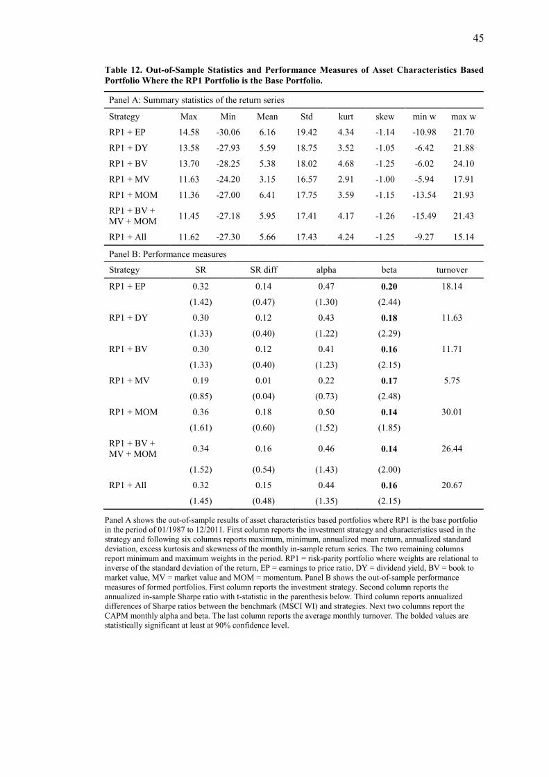
45
Table 12. Out-of-Sample Statistics and Performance Measures of Asset Characteristics Based
Portfolio Where the RP1 Portfolio is the Base Portfolio.
Panel A: Summary statistics of the return series
Strategy Max Min Mean Std kurt skew min w max w
RP1 + EP 14.58 -30.06 6.16 19.42 4.34 -1.14 -10.98 21.70
RP1 + DY 13.58 -27.93 5.59 18.75 3.52 -1.05 -6.42 21.88
RP1 + BV 13.70 -28.25 5.38 18.02 4.68 -1.25 -6.02 24.10
RP1 + MV 11.63 -24.20 3.15 16.57 2.91 -1.00 -5.94 17.91
RP1 + MOM 11.36 -27.00 6.41 17.75 3.59 -1.15 -13.54 21.93
RP1 + BV +
MV + MOM 11.45 -27.18 5.95 17.41 4.17 -1.26 -15.49 21.43
RP1 + All 11.62 -27.30 5.66 17.43 4.24 -1.25 -9.27 15.14
Panel B: Performance measures
Strategy SR SR diff alpha beta turnover
RP1 + EP 0.32 0.14 0.47 0.20 18.14
(1.42) (0.47) (1.30) (2.44)
RP1 + DY 0.30 0.12 0.43 0.18 11.63
(1.33) (0.40) (1.22) (2.29)
RP1 + BV 0.30 0.12 0.41 0.16 11.71
(1.33) (0.40) (1.23) (2.15)
RP1 + MV 0.19 0.01 0.22 0.17 5.75
(0.85) (0.04) (0.73) (2.48)
RP1 + MOM 0.36 0.18 0.50 0.14 30.01
(1.61) (0.60) (1.52) (1.85)
RP1 + BV +
MV + MOM 0.34 0.16 0.46 0.14 26.44
(1.52) (0.54) (1.43) (2.00)
RP1 + All 0.32 0.15 0.44 0.16 20.67
(1.45) (0.48) (1.35) (2.15)
Panel A shows the out-of-sample results of asset characteristics based portfolios where RP1 is the base portfolio
in the period of 01/1987 to 12/2011. First column reports the investment strategy and characteristics used in the
strategy and following six columns reports maximum, minimum, annualized mean return, annualized standard
deviation, excess kurtosis and skewness of the monthly in-sample return series. The two remaining columns
report minimum and maximum weights in the period. RP1 = risk-parity portfolio where weights are relational to
inverse of the standard deviation of the return, EP = earnings to price ratio, DY = dividend yield, BV = book to
market value, MV = market value and MOM = momentum. Panel B shows the out-of-sample performance
measures of formed portfolios. First column reports the investment strategy. Second column reports the
annualized in-sample Sharpe ratio with t-statistic in the parenthesis below. Third column reports annualized
differences of Sharpe ratios between the benchmark (MSCI WI) and strategies. Next two columns report the
CAPM monthly alpha and beta. The last column reports the average monthly turnover. The bolded values are
statistically significant at least at 90% confidence level.