NILMTK: An Open Source Toolkit for Non-intrusive LoadMonitoring

Nipun Batra1, Jack Kelly2, Oliver Parson3, Haimonti Dutta4, William Knottenbelt2,Alex Rogers3, Amarjeet Singh1, Mani Srivastava5

1Indraprastha Institute of Information Technology Delhi, India {nipunb, amarjeet}@iiitd.ac.in2 Imperial College London {jack.kelly, w.knottenbelt}@imperial.ac.uk

3 University of Southampton {osp, acr}@ecs.soton.ac.uk4 CCLS Columbia {haimonti@ccls.columbia.edu}

5 UCLA {mbs@ucla.edu}

ABSTRACTNon-intrusive load monitoring, or energy disaggregation,

aims to separate household energy consumption data col-lected from a single point of measurement into appliance-level consumption data. In recent years, the field has rapidlyexpanded due to increased interest as national deploymentsof smart meters have begun in many countries. However,empirically comparing disaggregation algorithms is currentlyvirtually impossible. This is due to the different data setsused, the lack of reference implementations of these algo-rithms and the variety of accuracy metrics employed. Toaddress this challenge, we present the Non-intrusive LoadMonitoring Toolkit (NILMTK); an open source toolkit de-signed specifically to enable the comparison of energy disag-gregation algorithms in a reproducible manner. This workis the first research to compare multiple disaggregation ap-proaches across multiple publicly available data sets. Ourtoolkit includes parsers for a range of existing data sets, acollection of preprocessing algorithms, a set of statistics fordescribing data sets, two reference benchmark disaggregationalgorithms and a suite of accuracy metrics. We demonstratethe range of reproducible analyses which are made possibleby our toolkit, including the analysis of six publicly availabledata sets and the evaluation of both benchmark disaggrega-tion algorithms across such data sets.

Categories and Subject DescriptorsI.5 [Pattern Recognition]: Applications

; I.2 [Artificial Intelligence]: Learning—Parameter learn-ing

Keywordsenergy disaggregation; non-intrusive load monitoring; smartmeters

To appear in the fifth International Conference on Future Energy Systems(ACM e-Energy), Cambridge, UK. 2014

1. INTRODUCTIONNon-intrusive load monitoring (NILM), or energy disaggre-gation, aims to break down a household’s aggregate electric-ity consumption into individual appliances [1]. The moti-vations for such a process are threefold. First, informing ahousehold’s occupants of how much energy each applianceconsumes empowers them to take steps towards reducingtheir energy consumption [2]. Second, personalised feed-back can be provided which quantifies the savings of certainappliance-specific advice, such as the financial savings whenan old inefficient appliance is replaced by a new efficient ap-pliance. Third, if the NILM system is able to determine thetime of use of each appliance, a recommender system wouldbe able to inform the household’s occupants of the savingsof deferring appliance use to a time of day when electricityis either cheaper or has a lower carbon footprint.

Such benefits have drawn significant interest in the fieldsince its inception 25 years ago. In recent years, the combi-nation of smart meter meter deployments [3, 4] and reducedhardware costs of household electricity sensors has led to arapid expansion of the field. Such rapid growth over thepast five years has been evidenced by the wealth of aca-demic papers published, international meetings held (e.g.NILM 20121 and EPRI NILM 20132), startup companiesfounded (e.g. Bidgely and Neurio) and data sets released,(e.g. REDD [5], BLUED [6] and Smart* [7]).

However, three core obstacles currently prevent the directcomparison of state-of-the-art approaches, and as a resultmay be impeding progress within the field. To the best ofour knowledge, each contribution to date has only been eval-uated on a single data set and consequently it is hard to as-sess whether such approaches generalise to new households.Furthermore, many researchers sub-sample data sets to se-lect specific households, appliances and time periods, mak-ing experimental results more difficult to reproduce. Second,newly proposed approaches are rarely compared against thesame benchmark algorithms, further increasing the difficultyin empirical comparisons of performance between differentpublications. Moreover, the lack of reference implementa-tions of these state-of-the-art algorithms often leads to thereimplementation of such approaches. Third, many paperstarget different use cases for NILM and therefore the ac-curacy of their proposed approaches are evaluated using adifferent set of performance metrics. As a result the nu-

1http://www.ices.cmu.edu/psii/nilm/2http://goo.gl/dr4tpq

arX

iv:1

404.

3878

v1 [

stat

.AP]

15

Apr

201

4

merical performance calculated by such metrics cannot becompared between any two papers. These three obstacleshave led to the proposal of successive extensions to state-of-the-art algorithms, while a direct comparison between newand existing approaches remains impossible.

Similar obstacles have arisen in other research fields andprompted the development of toolkits specifically designedto support research in that area. For example, PhysioToolkitoffers access to over 50 databases of physiological data andprovides software to support the processing and analysis ofsuch data for the biomedical research community [8]. Sim-ilarly, CRAWDAD collects 89 data sets of wireless networkdata in addition to software to aid the analysis of such datafor the wireless network community [9]. However, no suchtoolkit is available to the NILM community.

Against this background, we propose NILMTK3; an opensource toolkit designed specifically to enable easy accessto and comparative analysis of energy disaggregation algo-rithms across diverse data sets. NILMTK provides a com-plete pipeline from data sets to accuracy metrics, therebylowering the entry barrier for researchers to implement a newalgorithm and compare its performance against the currentstate of the art. NILMTK has been:

• released as open source software (with documentation4)in an effort to encourage researchers to contribute datasets, benchmark algorithms and accuracy metrics asthey are proposed, with the goal of enabling a greaterlevel of collaboration within the community.

• designed using a modular structure, therefore allow-ing researchers to reuse or replace individual compo-nents as required. The API design is influenced byscikit-learn [10], which is a machine learning libraryin Python, well known for its consistent API and com-plete documentation.

• written in Python with flat file input and output for-mats, in addition to high performance binary formats,ensuring compatibility with existing algorithms writ-ten in any language and designed for any platform.

The contributions of NILMTK are summarised as follows:

• We propose NILMTK-DF (data format), the standardenergy disaggregation data structure used by our toolkit.NILMTK-DF is modelled loosely on the REDD dataset format [5] to allow easy adoption within the com-munity. Furthermore, we provide parsers from six ex-isting data sets into our proposed NILMTK-DF for-mat.

• We provide statistical and diagnostic functions whichprovide a detailed understanding of each data set. Wealso provide preprocessing functions for mitigating com-mon challenges with NILM data sets.

• We provide implementations of two benchmark disag-gregation algorithms: first an approach based on com-binatorial optimisation [1], and second an approachbased on the factorial hidden Markov model [5, 11].We demonstrate the ease by which NILMTK allows

3Code: http://github.com/nilmtk/nilmtk (release v0.1.0was used for this paper)4Documentation: http://nilmtk.github.io/nilmtk

the comparison of these algorithms across a range ofexisting data sets, and present results of their perfor-mance.

• We present a suite of accuracy metrics which enablesthe evaluation of any disaggregation algorithm com-patible with NILMTK. This allows the performance ofa disaggregation algorithm to be evaluated for a rangeof use cases.

The remainder of this paper is organised as follows. InSection 2 we provide an overview of related work. In Sec-tion 3 we present NILMTK and describe its components. InSection 4 we demonstrate the empirical evaluations whichare enabled by NILMTK, and provide analyses of existingdata sets and disaggregation algorithms. Finally, in Sec-tion 5 we conclude the paper and propose directions for fu-ture work.

2. BACKGROUNDThe field of non-intrusive load monitoring was founded 25years ago when Hart proposed the first algorithm for the dis-aggregation of household energy usage [1, 12]. However, themajority of research prior to 2011 had been evaluated usingeither lab-based or simulated data and hence the perfor-mance of disaggregation algorithms in real households hadremained unknown. More recently, national deployments ofsmart meters have prompted a renewed interest in energydisaggregation. We now discuss recent research which hascontributed new data sets (Section 2.1), disaggregation algo-rithms (Section 2.2) and evaluation metrics (Section 2.3) tothe field. In Section 2.4 we discuss general purpose toolkits,and finally in Section 2.5 we formalise the NILM problemdrawing upon notation used in prior literature.

2.1 Public Data SetsIn 2011, the Reference Energy Disaggregation Dataset (REDD)[5] was introduced as the first publicly available data setcollected specifically to aid NILM research. The data setcontains both aggregate and sub-metered power data fromsix households, and has since become the most popular dataset for evaluating energy disaggregation algorithms. In 2012,the Building-Level fUlly-labeled dataset for Electricity Dis-aggregation (BLUED) [6] was released containing data froma single household. However, the data set does not includesub-metered power data, and instead records events trig-gered by appliance state changes. As a result, it is only pos-sible to evaluate whether changes in appliance states havebeen detected (e.g. washing machine turns on), rather thanthe assignment of aggregate power demand to individual ap-pliances (e.g. washing machine draws 2 kW power). Morerecently, the Smart* [7] data set was released, which con-tains household aggregate power data from three households,while sub-metered appliance power data was only collectedfrom a single household.

In 2013 the Pecan Street sample data set was released [13],which contains both aggregate and sub-metered power datafrom 10 households. Later, the Household Electricity Sur-vey data set was released [14], which contains data from251 households although aggregate data was only collectedfor 14 households. The Almanac of Minutely Power dataset(AMPds) [15] was also released that year containing bothaggregate and sub-metered power data from a single house-hold. Subsequently, the Indian data for Ambient Water and

Duration Number Appliance AggregateData set Institution Location per of sample sample

house houses frequency frequencyREDD (2011) MIT MA, USA 3-19 days 6 3 sec 1 sec & 15 kHz

BLUED (2012) CMU PA, USA 8 days 1 N/A* 12 kHzSmart* (2012) UMass MA, USA 3 months 3 1 sec 1 sec

Tracebase (2012) Darmstadt Germany N/A N/A 1-10 sec N/ASample (2013) Pecan Street TX, USA 7 days 10 1 min 1 min

HES (2013) DECC, DEFRA UK 1 or 12 months 251 2 or 10 min 2 or 10 minAMPds (2013) Simon Fraser U. BC, Canada 1 year 1 1 min 1 miniAWE (2013) IIIT Delhi Delhi, India 73 days 1 1 or 6 sec 1 sec

UK-DALE (2014) Imperial College London, UK 3-17 months 4 6 sec 1-6 sec & 16 kHz

Table 1: Comparison of household energy data sets. *BLUED labels state transitions for each appliance.

Electricity Sensing (iAWE) [16] was released, which containsboth aggregate and sub-metered power data from a singlehouse. Most recently, the UK Domestic Appliance-LevelElectricity data set [17] (UK-DALE) was released which con-tains data from four households using both aggregate metersand individual appliance sub-meters. Unfortunately, subtledifferences in the aims of each data set have led to com-pletely different data formats being used. As a result, atime-consuming engineering barrier exists when using thedata sets, each of which are in different formats. This hasresulted in publications using only a single data set to eval-uate a given approach, and consequently the generality ofresults over large numbers of households are rarely investi-gated. We summarise these data sets in Table 1.

2.2 Disaggregation Algorithms & BenchmarksThe REDD data set was proposed along with a performanceresult of a benchmark disaggregation algorithm using 10 sec-ond data across five of the six households [5]. Kolter andJaakkola later proposed an extension to the benchmark al-gorithm [18], however the extension was only evaluated us-ing features extracted from 15 kHz data from a single housefrom the data set, and therefore the performance resultsare not directly comparable. Later, Zeifman [19] and John-son and Willsky [20] evaluated various approaches using thesame data set, although both selected a different subset ofappliances and calculated an artificial household aggregatefrom these appliances, therefore simplifying the disaggrega-tion problem and preventing a numerical comparison withother publications. Subsequently, Parson et al. [21] and Ra-hayu et al. [22] both proposed new approaches, althougheach were evaluated using a different set of four houses fromthe REDD data set, again preventing a numerical compar-ison between publications. Last, Batra et al. [23] evalu-ated their approach on the REDD data set using a differenthousehold to Kolter and Jaakkola. As a result, it has notbeen possible to deduce whether one approach is preferableto another from the literature.

The BLUED data set was introduced along with a bench-mark algorithm [6], but has since only been used by oneother publication [24]. Similarly, AMPds has only been usedto evaluate disaggregation algorithms proposed by the dataset authors [15]. Clearly, the variety of different formats isslowing the uptake of new data sets, and also preventingalgorithms from being tested across multiple data sets.

It is essential to compare newly proposed disaggregationalgorithms to the state of the art in order to assess the in-

crease in an algorithm’s performance. However, the lack ofavailable reference implementations of state-of-the-art dis-aggregation algorithms has led to authors often comparingagainst more basic benchmark algorithms. This problemis further compounded since there is no single consensuson which benchmarks to use, and as a result most publi-cations use a different benchmark algorithm. For example,Kolter and Jaakkola compared their approach to a set ofdecoupled HMMs [18], Parson et al. and Batra et al. bothevaluated their approaches against variants of their own ap-proaches [21, 23], Zeifman compared their approach to aBayesian classifier, while Rahayu et al. and Johnson andWillsky both compared against a factorial hidden Markovmodel (FHMM) [22, 20]. Clearly, further publications wouldbenefit from openly available benchmark algorithms againstwhich newly proposed algorithms could be easily compared.

2.3 Evaluation MetricsThe range of different application areas of energy disaggre-gation has prompted a number of evaluation metrics to beproposed. For example, four disaggregation metrics labelledenergy correctly assigned have recently been used to evalu-ate the performance of disaggregation algorithms using theREDD data set. First, Kolter and Johnson [5] proposed anaccuracy metric which captures the error in assigned energynormalised by the actual energy consumption in each timeslice averaged over all appliances, which was also later usedby Rahayu et al. [22] and Johnson and Willsky [20]. How-ever, large errors in the assigned energy in some time sliceswill result in a negative accuracy, making this an ill-posedmetric. Second, Kolter and Jaakkola [18] proposed an equiv-alent metric wherein the error is presented individually foreach appliance rather than an average across all appliances.Third, Parson et al. [21] proposed a metric which capturesthe error in assigned energy consumed over the complete du-ration of the data set rather than per time slice. This met-ric allows overestimates and underestimates in the assignedenergy in different time slices to cancel out, and thereforedoes not represent all disaggregation errors. Fourth, Batraet al. [23] proposed a subtly different metric to Kolter andJohnson [5], in which error is reported instead of accuracy,and also energy assigned to an incorrect appliance is doublecounted as both an overestimate of one appliance’s energyconsumption and an underestimate of another. The differ-ences between these four metrics prevent numerical compar-isons between publications, and motivate the use of commonmetrics.

Disaggregation

Data interface

NILMTK-DF Preprocessing

Statistics Training Model

MetricsUK-DALE

BLUED

REDD

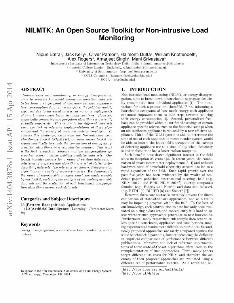
Figure 1: NILMTK pipeline. At each stage of the pipeline, results and data can be stored to or loaded from disk.

2.4 General Purpose ToolkitsAlthough no toolkit currently exists specifically for energydisaggregation, various toolkits are available for more gen-eral machine learning tasks. For example, scikit-learn isa general purpose machine learning toolkit implemented inPython [10] and GraphLab is a machine learning and datamining toolkit written in C++ [25]. While such toolkitsprovide generic implementations of machine learning algo-rithms, they lack functionality specific to the energy disag-gregation domain, such as data set parsers, benchmark dis-aggregation algorithms, and energy disaggregation metrics.Therefore, an energy disaggregation toolkit should extendsuch general toolkits rather than replace them, in a similarway that scikit-learn adds machine learning functionalityto the numpy numerical library for Python.

2.5 Energy Disaggregation DefinitionThe aim of energy disaggregation is to provide estimates,

y(n)t , of the actual power demand, y

(n)t , of each appliance n at

time t, from household aggregate power readings, yt. MostNILM algorithms model appliances using a set of discrete

states such as off, on, intermediate, etc. We use x(n)t ∈ Z>0

to represent the ground truth state, and x(n)t to represent

the appliance state estimated by a disaggregation algorithm.

3. NILMTKWe designed NILMTK with two core use cases in mind.First, it should enable the analysis of existing data sets andalgorithms. Second, it should provide a simple interface forthe addition of new data sets and algorithms. To do so, weimplemented NILMTK in Python due to the availability ofa vast set of libraries supporting both machine learning re-search (e.g. Pandas, scikit-learn) and the deployment ofsuch research as web applications (e.g. Django). Further-more, Python allows easy deployment in diverse environ-ments including academic settings and is increasingly beingused for data science.

Figure 1 presents the NILMTK pipeline from the importof data sets to the evaluation of various disaggregation algo-rithms over various metrics. In Appendix A we summarisethe NILMTK pipeline with an illustrative code snippet. Inthe remainder of this section we discuss each module of thepipeline: the NILMTK data format, the data set diagnosticsand statistics, preprocessing, disaggregation, model importand export and finally we describe accuracy metrics.

3.1 Data FormatMotivated by our discussion in Section 2.1 of the wide dif-ferences between multiple data sets released in the publicdomain, we propose NILMTK-DF; a common data set for-mat inspired by the REDD format [5], into which existingdata sets can be converted. NILMTK currently includesimporters for the following six data sets: REDD, Smart*,Pecan Street, iAWE, AMPds and UK-DALE. BLUED wasexcluded due to the lack of sub-metered power data, theTracebase data set was excluded due to the lack of house-hold aggregate power data and HES was excluded due totime constraints.

After import, the data resides in our NILMTK-DF in-memory data structure, which is used throughout the NILMTKpipeline. Data can be saved or loaded from disk at multiplestages in the NILMTK processing pipeline to allow othertools to interact with NILMTK. We provide two CSV flatfile formats: a rich NILMTK-DF CSV format and a “strictREDD” format which allows researchers to use their exist-ing tools designed to process REDD data. We also providea more efficient binary format using the Hierarchical DataFormat (HDF5). In addition to storing electricity data,NILMTK-DF can also store relevant metadata and othersensor modalities such as gas, water, temperature, etc. Ithas been shown that such additional sensor and metadatainformation may help enhance NILM prediction [26].

Another important feature of our format is the standard-isation of nomenclature. Different data sets use differentlabels for the same class of appliance (e.g. REDD uses ‘re-frigerator’ whilst AMPds uses ‘FGE’) and different namesfor the measured parameters. When data is first importedinto NILMTK, these diverse labels are converted to a stan-dard vocabulary [27].

In addition, NILMTK allows rich metadata to be associ-ated with a household, appliance or meter. For example,NILMTK can store the parameters measured by each meter(e.g. reactive power, real power), the geographical coordi-nates of each house (to enable weather data to be retrieved),the mains wiring defining the meter hierarchy (useful if asingle appliance is measured at the appliance, circuit andaggregate levels), whether a single meter measures multipleappliances and whether a specific lamp is dimmable. Moredetail is provided in Appendix B and our full NILM Meta-data schema is described in [27].

Through such a combination of metadata and standardnomenclature, NILMTK allows for analysis of appliance dataacross multiple data sets. For example, users can perform

queries such as: ‘what is the energy consumption of refriger-ators in the USA compared to the UK?’. Further examplesare given in Appendix C.

We have defined a common interface for data set importerswhich, combined with the definition of our in-memory datastructures, enables developers to easily add new data setimporters to NILMTK.

3.2 Data Set DiagnosticsSince no data set is perfect, researchers are required to ex-plore the characteristics of each data set before disaggrega-tion approaches can be evaluated. To help diagnose theseissues, NILMTK provides diagnostic functions including:

Detect gaps: Many NILM algorithms assume that eachsensor channel is contiguous. However, this assumption isviolated when sensors are off or malfunctioning. A ‘gap’exists between any pair of consecutive samples if the timeelapsed between them is larger than a predefined threshold.

Dropout rate: The dropout rate is the total number ofrecorded samples, divided by the number of expected sam-ples (which is the length of the time window under consid-eration multiplied by the sample rate).

Dropout rate (ignoring gaps): To quantify the rateat which a wireless sensor drops samples due to radio is-sues, we first remove large gaps where the sensor is off andsubsequently calculate the dropout rate for the remainingcontiguous sections.

Up-time: The up-time is the total time for which a sen-sor was recording. It is the last timestamp, minus the firsttimestamp, minus the duration of any gaps.

Diagnose: NILMTK provides a single diagnose functionwhich checks for all the issues we have encountered.

3.3 Data Set StatisticsDistinct from diagnostic statistics, NILMTK also providesfunctions for exploring appliance usage, e.g.:

Proportion of energy sub-metered: Data sets rarelysub-meter every appliance or circuit, and as a result it isuseful to quantify the proportion of total energy measured bysub-metered channels. Prior to calculating this statistic, allgaps present in the mains recordings are masked out of eachsub-metered channel, and therefore any additional missingsub-meter data is assumed to be due to the meter and loadbeing switched off.

Section 3.2 and 3.3 have described a subset of the diagnos-tic and statistical functions in NILMTK. Further functionsare listed in Appendix D and in the statistics section of theonline documentation.5

3.4 Preprocessing of Data SetsTo mitigate the problems with different data sets, some ofwhich were presented in Section 3.2, NILMTK provides sev-eral preprocessing functions, including:

Downsample: As seen in Table 1, the sampling rate ofappliance monitors varies from 0.008 Hz to 16 kHz acrossthe data sets. The downsample preprocessor down-samplesdata sets to a specified frequency using aggregation functionssuch as mean, mode and median.

Voltage normalisation: The data sets presented in Ta-ble 1 have been collected from different countries, wherevoltage fluctuations vary widely. Batra et al. showed volt-age fluctuates from 180-250 V in the iAWE data set collected

5 http://nilmtk.github.io/nilmtk/stats.html

in India [16], while the voltage in the Smart* data set variesacross the range 118-123 V. Hart suggested to account forthese voltage fluctuations as they can significantly impactpower draw [1]. Therefore, NILMTK provides a voltage nor-malisation function based on Hart’s equation:

Powernormalised =

(Voltagenominal

Voltageobserved

)2

× Powerobserved (1)

Top-k appliances: It is often advantageous to model thetop-k energy consuming appliances instead of all appliancesfor the following three reasons. First, the disaggregation ofsuch appliances provides the most value. Second, such appli-ances contribute the most salient features, and therefore theremaining appliances can be considered to contribute onlynoise. Third, each additional modelled appliance might con-tribute significantly to the complexity of the disaggregationtask. Therefore, NILMTK provides a function to identifythe top-k energy consuming appliances.

NILMTK also provides preprocessing functions for fixingother common issues with these data sets, such as: (i) in-terpolating small periods of missing data when appliancesensors did not report readings, (ii) filtering out implausi-ble values (such as readings where observed voltage is morethan twice the rated voltage) and (iii) filtering out appliancedata when mains data is missing.

Each data set importer defines a preprocess functionwhich runs the necessary preprocessing functions to cleanthe specific data set. A detailed account of preprocess-ing functions supported by NILMTK can be found in Ap-pendix D and in the online documentation.6

3.5 Training and Disaggregation AlgorithmsNILMTK provides implementations of two common bench-mark disaggregation algorithms: combinatorial optimisation(CO) and factorial hidden Markov model (FHMM). CO wasproposed by Hart in his seminal work [1], while techniquesbased on extensions of the FHMM have been proposed morerecently [5, 11]. The aim of the inclusion of these algorithmsis not to present state-of-the-art disaggregation results, butinstead to enable new approaches to be compared to well-studied benchmark algorithms without requiring the reim-plementation of such algorithms. We now describe these twoalgorithms.

Combinatorial Optimisation: CO finds the optimalcombination of appliance states, which minimises the differ-ence between the sum of the predicted appliance power andthe observed aggregate power, subject to a set of appliancemodels.

x(n)t = argmin

x(n)t

∣∣∣∣∣yt −N∑n=1

y(n)t

∣∣∣∣∣ (2)

Since each time slice is considered as a separate optimi-sation problem, each time slice is assumed to be indepen-dent. CO resembles the subset sum problem and thus isNP-complete. The complexity of disaggregation for T timeslices is O(TKN ), where N is the number of appliances andK is the number of appliance states. Since the complexityof CO is exponential in the number of appliances, the ap-proach is only computationally tractable for a small numberof modelled appliances.

6 http://nilmtk.github.io/nilmtk/preprocessing.html

Factorial Hidden Markov Model: The power demandof each appliance can be modelled as the observed value ofa hidden Markov model (HMM). The hidden component ofthese HMMs are the states of the appliances. Energy dis-aggregation involves jointly decoding the power draw of nappliances and hence a factorial HMM [28] is well suited. AFHMM can be represented by an equivalent HMM in whicheach state corresponds to a different combination of states ofeach appliance. Such a FHMM model has three parameters:(i) prior probability (π) containing KN entries, (ii) transi-tion matrix (A) containing KN ×KN or K2N entries, and(iii) emission matrix (B) containing 2KN entries. The com-plexity of exact disaggregation for such a model isO(TK2N ),and as a result FHMMs scale even worse than CO. From animplementation perspective, even storing (or computing) Afor 14 appliances with two states each consumes 8 GB ofRAM. Hence, we propose to validate FHMMs on prepro-cessed data where the top-k appliances are modelled, andappliances contributing less than a given threshold are dis-carded. However, it should be noted that more efficientpseudo-time algorithms could alternatively be used for in-ference over both CO and FHMM.

For algorithms such as FHMMs, it is necessary to modelthe relationships amongst consecutive samples. Thus, NILMTKprovides facilities for dividing data into continuous sets fortraining and testing. While we have discussed supervisedand non-event based algorithms here, NILMTK also sup-ports event based and unsupervised approaches. Details foradding new algorithms are provided in Appendix E.

3.6 Appliance Model Import and ExportMany approaches require sub-metered power data to be col-lected for training purposes from the same household inwhich disaggregation is to be performed. However, suchdata is costly and intrusive to collect, and therefore is un-likely to be available in a large-scale deployment of a NILMsystem. As a result, recent research has proposed trainingmethods which do not require sub-metered power data to becollected from each household [11, 21]. To provide a clearinterface between training and disaggregation algorithms,NILMTK provides a model module which encapsulates theresults of the training module required by the disaggregationmodule. Each implementation of the module must provideimport and export functions to interface with a JSON filefor persistent model storage. NILMTK currently includesimporters and exporters for both the FHMM and CO ap-proaches described in Section 3.5.

3.7 Accuracy MetricsAs discussed in Section 2.3, a range of accuracy metricsare required due to the diversity of application areas of en-ergy disaggregation research. To satisfy this requirement,NILMTK provides a set of metrics which combines bothgeneral detection metrics and those specific to energy dis-aggregation. We now give a brief description of each metricimplemented in NILMTK along with its mathematical defi-nition.

Error in total energy assigned: The difference be-tween the total assigned energy and the actual energy con-sumed by appliance n over the entire data set.∣∣∣∣∣∑

t

y(n)t −

∑t

y(n)t

∣∣∣∣∣ (3)

Fraction of total energy assigned correctly: Theoverlap between the fraction of energy assigned to each ap-pliance and the actual fraction of energy consumed by eachappliance over the data set.∑

n

min

( ∑n y

(n)t∑

n,t y(n)t

,

∑n y

(n)t∑

n,t y(n)t

)(4)

Normalised error in assigned power: The sum of thedifferences between the assigned power and actual power ofappliance n in each time slice t, normalised by the appli-ance’s total energy consumption.∑

t

∣∣∣y(n)t − y(n)t

∣∣∣∑t y

(n)t

(5)

RMS error in assigned power: The root mean squareerror between the assigned power and actual power of appli-ance n in each time slice t.√

1

T

∑t

(y(n)t − y(n)t

)2(6)

Confusion matrix: The number of time slices in whicheach of an appliance’s states were either confused with everyother state or correctly classified.

True positives, False positives, False negatives, Truenegatives: The number of time slices in which appliance nwas either correctly classified as being on (TP), classifiedas being on while it was actually off (FP), classified as offwhile is was actually on (FN ) and correctly classified as be-ing off (TN ).

TP (n) =∑t

AND(x(n)t = on, x

(n)t = on

)(7)

FP (n) =∑t

AND(x(n)t = off , x

(n)t = on

)(8)

FN (n) =∑t

AND(x(n)t = on, x

(n)t = off

)(9)

TN (n) =∑t

AND(x(n)t = off , x

(n)t = off

)(10)

True/False positive rate: The fraction of time slicesin which an appliance was correctly predicted to be on thatit was actually on (TPR), and the fraction of time slices inwhich the appliance was incorrectly predicted to be on thatit was actually off (FPR). We omit appliance indices n inthe following metrics for clarity.

TPR =TP

(TP + FN )(11)

FPR =FP

(FP + TN )(12)

Precision, Recall: The fraction of time slices in whichan appliance was correctly predicted to be on that it wasactually off (Precision), and the fraction of time slices inwhich the appliance was correctly predicted to be on that itwas actually on (Recall).

Precision =TP

(TP + FP)(13)

Data setNumber ofappliances

Percentageenergy

sub-metered

Dropout rate(percent)

ignoring gaps

Mains up-timeper house

(days)

Percentageup-time

REDD 9, 16, 23 58, 71, 89 0, 10, 16 4, 18, 19 8, 40, 79Smart* 25 86 0 88 96

Pecan Street 13, 14, 22 75, 87, 150 0, 0, 0 7, 7, 7 100, 100, 100AMPds 20 97 0 364 100iAWE 10 48 8 47 93

UK-DALE 4, 12, 53 19, 48, 82 0, 7, 22 36, 102, 470 73, 84, 100

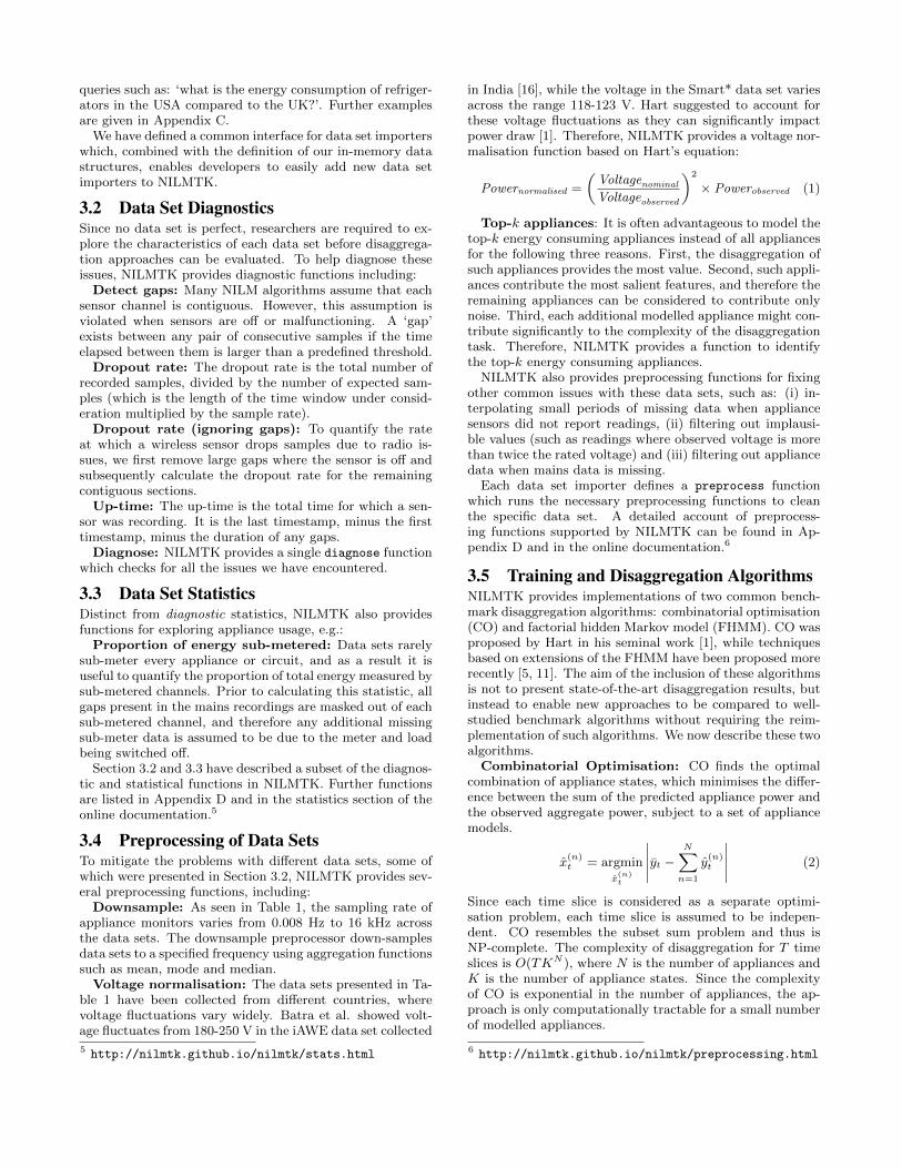
Table 2: Summary of data set results calculated by the diagnostic and statistical functions in NILMTK. Each cellrepresents the range of values across all households per data set. The three numbers per cell are the minimum, medianand maximum values. AMPds, Smart* and iAWE each contain just a single house, hence these rows have a singlenumber per cell.

18/04/11 06/05/11 24/05/11Time (day/month/year)

Fridge

Washer dryer

Kitchen outlets

Mains 1

Mains 2

0

10

≥ 20

Dro

pout

rate

(%)

Figure 2: Lost samples per hour from a representativesubset of channels in REDD house 1.

Recall =TP

(TP + FN )(14)

F-score: The harmonic mean of precision and recall.

F -score =2.Precision.Recall

Precision + Recall(15)

Hamming loss: The total information lost when appli-ances are incorrectly classified over the data set.

HammingLoss =1

T

∑t

1

N

∑n

XOR(x(n)t , x

(n)t

)(16)

4. EVALUATIONWe now demonstrate several examples of the rich analysessupported by NILMTK. First, we diagnose some common(and inevitable) issues in a selection of data sets. Second,we show various patterns of appliance usage. Third, we givesome examples of the effect of voltage normalisation on thepower demand of individual appliances, and discuss how thismight affect the performance of a disaggregation algorithm.Fourth, we present summary performance results of the twobenchmark algorithms included in NILMTK across six datasets using a number of accuracy metrics. Finally, we presentdetailed results of these algorithms for a single data set, anddiscuss their performance for different appliances.

4.1 Data Set DiagnosticsTable 2 shows a selection of diagnostic and statistical func-tions (defined in Section 3.2 and 3.3) computed by NILMTKacross six public data sets. BLUED, Tracebase and HESwere not included for the same reasons as in Section 3.1.The table illustrates that AMPds used a robust recordingplatform because it has a percentage up-time of 100%, adropout rate of zero and 97% of the energy recorded by the

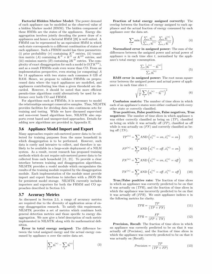
0 30 600

1

2

3

Act

ive

pow

er(k

W)

REDD

0 30 60

UK-DALE

Time (minutes)

Figure 3: Comparison of power draw of washing ma-chines in one house from REDD (USA) and UK-DALE.

mains channel was captured by the sub-meters. Similarly,Pecan Street has an up-time of 100% and zero dropout rate.However, two homes in the Pecan Street data registered aproportion of energy sub-metered of over 100%. This indi-cates that some overlap exists between the metered chan-nels, and as a result some appliances are metered by mul-tiple channels. This illustrates the importance of data setmetadata (proposed as part of NILMTK-DF in Section 3.1)describing the basic mains wiring.

Figure 2 shows the distribution of missing samples forREDD house 1. From this we can see that each mainsrecording channel has four large gaps (the solid black blocks)where the sensors are off. The sub-metered channels haveonly one large gap. Ignoring this gap and focusing on thetime periods where the sensors are recording, we see numer-ous periods where the dropout rate is around 10%. Suchissues are by no means unique to REDD and are crucial todiagnose before data sets can be used for the evaluation ofdisaggregation algorithms or for data set statistics.

4.2 Data Set StatisticsEnergy disaggregation systems must model individual ap-pliances. Hence, as well as diagnosing technical issues witheach data set, NILMTK also provides functions to visu-alise patterns of behaviour recorded in each data set. Forexample, different appliances draw a different amount ofpower (e.g. a toaster draws approximately 1.57 kW), areused at different times of day (e.g. the TV is usually onin the evening) and have different correlations with exter-nal factors such as weather (e.g. lower outside temperatureimplies more usage of electric heating). Furthermore, loadprofiles of different appliances of the same type can varyconsiderably, especially appliances from different countries(e.g. the two washing machine profiles in Figure 3). Some

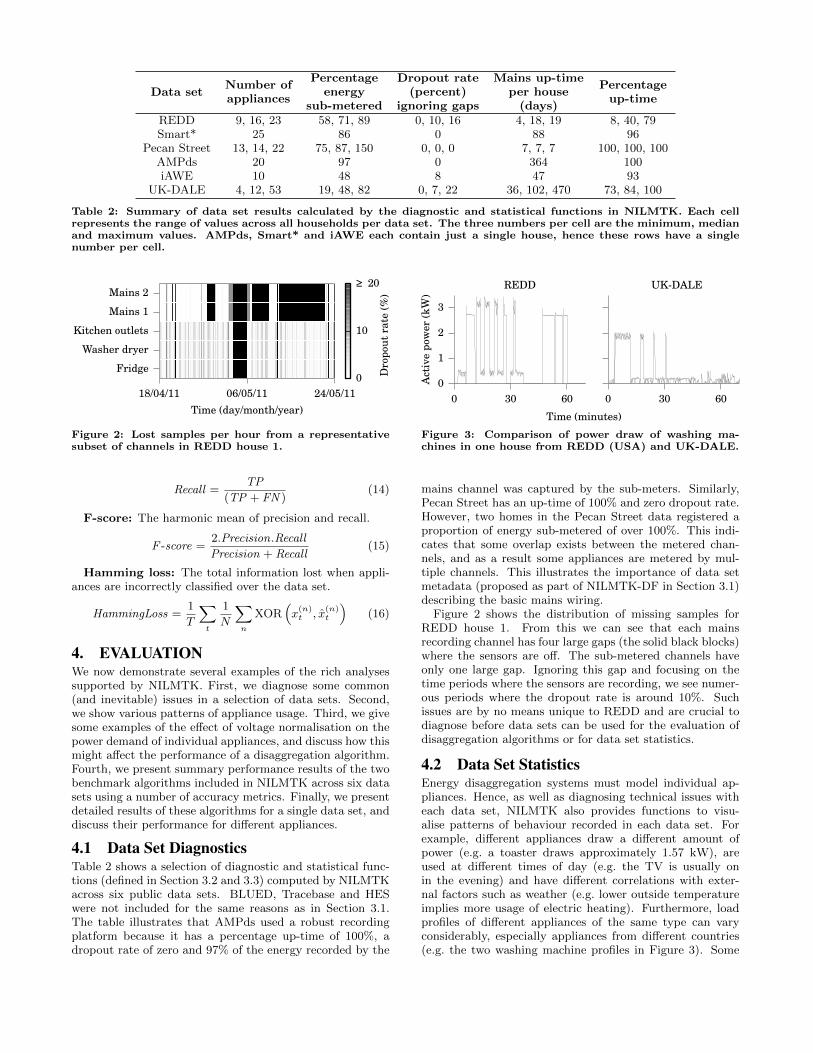
0.0 1.0 2.0

Fre

quen

cyWasher dryer

1.5 1.6

Toaster

0.1 0.2

Dimmable LED kitchen lights

1.6 1.8 2.0 2.2

Air conditioning

Active power (kW)

Figure 4: Histograms of power consumption. The filled grey plots show histograms of normalised power. The thin,grey, semi-transparent lines drawn over the filled plots show histograms of un-normalised power.

disaggregation systems benefit by capturing these patterns(for example, the conditional factorial hidden Markov model(CFHMM) [11] can model the influence of time of day onappliance usage). In the following sections, we present ex-amples of how such information can be extracted from ex-isting data sets using NILMTK, covering the distributionof appliance power demands (Section 4.2.1), usage patterns(Section 4.2.2) and external dependencies (Section 4.2.3).

4.2.1 Appliance power demandsFigure 4 displays histograms of the distribution of powersused by a selection of appliances (the washer dryer, toasterand dimmable LED kitchen lights are from UK-DALE house1; the air conditioning unit is from iAWE). Appliances suchas toasters and kettles tend to have just two possible powerstates: on and off. This simplicity makes them amenable tobe modelled by, for example, Markov chains with only twostates per chain. In contrast, more complex appliances suchas washing machines, vacuum cleaners and computers oftenhave many more states.

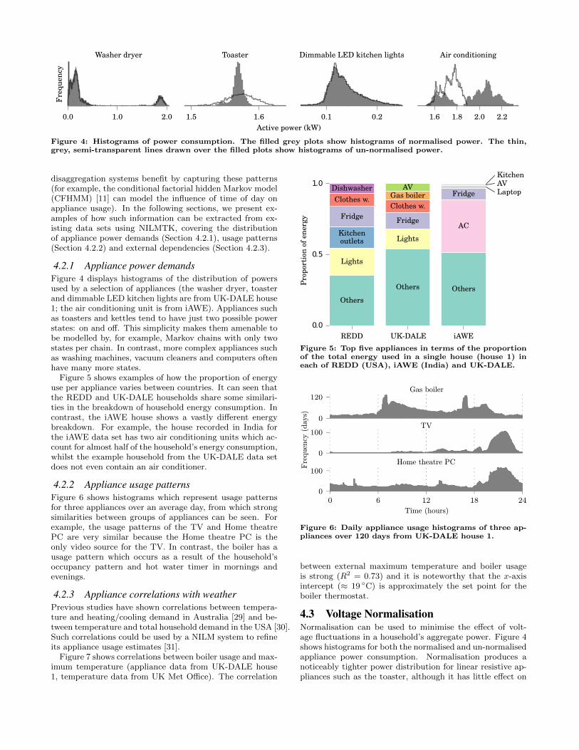
Figure 5 shows examples of how the proportion of energyuse per appliance varies between countries. It can seen thatthe REDD and UK-DALE households share some similari-ties in the breakdown of household energy consumption. Incontrast, the iAWE house shows a vastly different energybreakdown. For example, the house recorded in India forthe iAWE data set has two air conditioning units which ac-count for almost half of the household’s energy consumption,whilst the example household from the UK-DALE data setdoes not even contain an air conditioner.

4.2.2 Appliance usage patternsFigure 6 shows histograms which represent usage patternsfor three appliances over an average day, from which strongsimilarities between groups of appliances can be seen. Forexample, the usage patterns of the TV and Home theatrePC are very similar because the Home theatre PC is theonly video source for the TV. In contrast, the boiler has ausage pattern which occurs as a result of the household’soccupancy pattern and hot water timer in mornings andevenings.

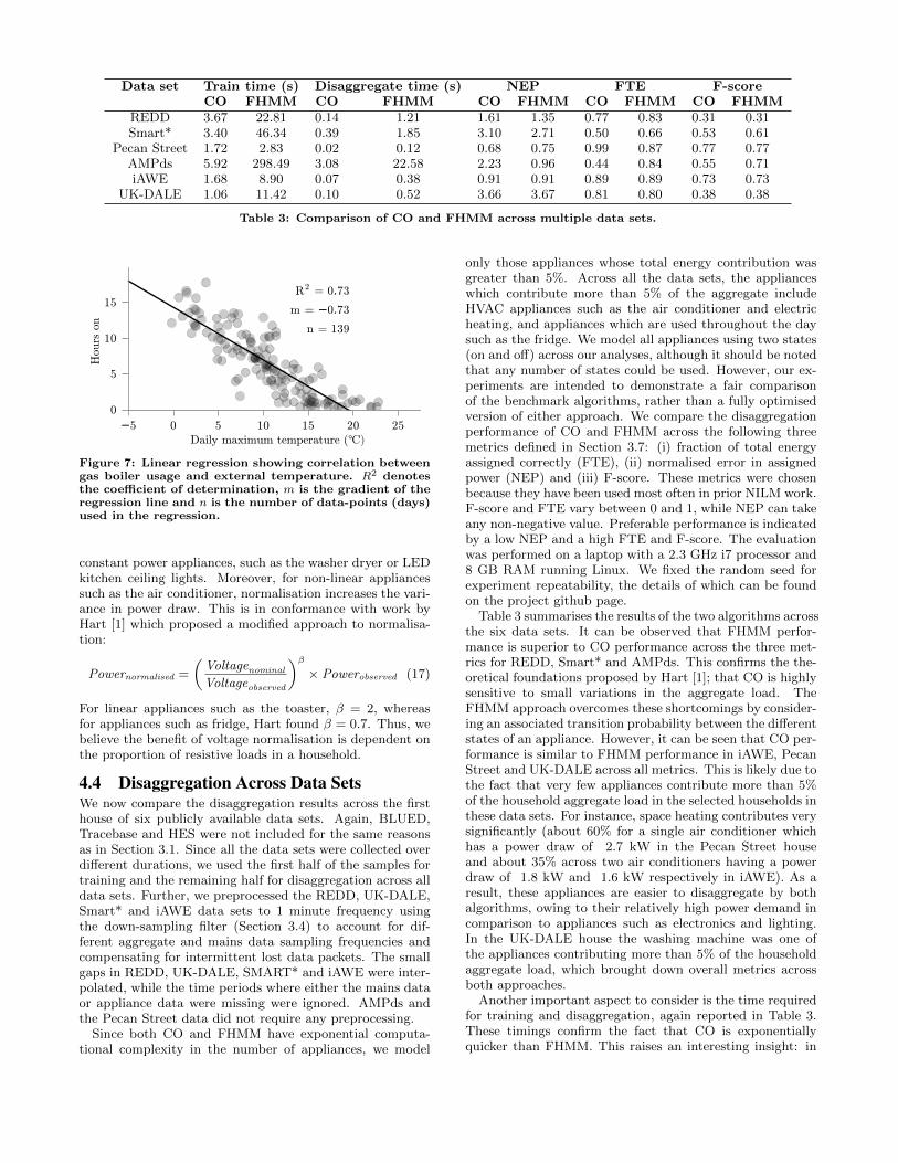
4.2.3 Appliance correlations with weatherPrevious studies have shown correlations between tempera-ture and heating/cooling demand in Australia [29] and be-tween temperature and total household demand in the USA [30].Such correlations could be used by a NILM system to refineits appliance usage estimates [31].

Figure 7 shows correlations between boiler usage and max-imum temperature (appliance data from UK-DALE house1, temperature data from UK Met Office). The correlation

REDD UK-DALE iAWE0.0

0.5

1.0

Pro

port

ion

ofen

ergy

Others

Others Others

Lights

Lights

ACKitchenoutlets

Fridge

Fridge

FridgeClothes w.

LaptopClothes w. Gas boiler

AVDishwasher AV

Kitchen

Figure 5: Top five appliances in terms of the proportionof the total energy used in a single house (house 1) ineach of REDD (USA), iAWE (India) and UK-DALE.

HHome theatre PC

TV

Gas boiler

Time (hours)

Fre

quen

cy (

days)

Figure 6: Daily appliance usage histograms of three ap-pliances over 120 days from UK-DALE house 1.

between external maximum temperature and boiler usageis strong (R2 = 0.73) and it is noteworthy that the x-axisintercept (≈ 19 ◦C) is approximately the set point for theboiler thermostat.

4.3 Voltage NormalisationNormalisation can be used to minimise the effect of volt-age fluctuations in a household’s aggregate power. Figure 4shows histograms for both the normalised and un-normalisedappliance power consumption. Normalisation produces anoticeably tighter power distribution for linear resistive ap-pliances such as the toaster, although it has little effect on

Data set Train time (s) Disaggregate time (s) NEP FTE F-scoreCO FHMM CO FHMM CO FHMM CO FHMM CO FHMM

REDD 3.67 22.81 0.14 1.21 1.61 1.35 0.77 0.83 0.31 0.31Smart* 3.40 46.34 0.39 1.85 3.10 2.71 0.50 0.66 0.53 0.61

Pecan Street 1.72 2.83 0.02 0.12 0.68 0.75 0.99 0.87 0.77 0.77AMPds 5.92 298.49 3.08 22.58 2.23 0.96 0.44 0.84 0.55 0.71iAWE 1.68 8.90 0.07 0.38 0.91 0.91 0.89 0.89 0.73 0.73

UK-DALE 1.06 11.42 0.10 0.52 3.66 3.67 0.81 0.80 0.38 0.38

Table 3: Comparison of CO and FHMM across multiple data sets.

−5 0 5 10 15 20 25

0

5

10

15R2 = 0.73

m = −0.73

n = 139

Daily maximum temperature (℃)

Hours

on

Figure 7: Linear regression showing correlation betweengas boiler usage and external temperature. R2 denotesthe coefficient of determination, m is the gradient of theregression line and n is the number of data-points (days)used in the regression.

constant power appliances, such as the washer dryer or LEDkitchen ceiling lights. Moreover, for non-linear appliancessuch as the air conditioner, normalisation increases the vari-ance in power draw. This is in conformance with work byHart [1] which proposed a modified approach to normalisa-tion:

Powernormalised =

(Voltagenominal

Voltageobserved

)β× Powerobserved (17)

For linear appliances such as the toaster, β = 2, whereasfor appliances such as fridge, Hart found β = 0.7. Thus, webelieve the benefit of voltage normalisation is dependent onthe proportion of resistive loads in a household.

4.4 Disaggregation Across Data SetsWe now compare the disaggregation results across the firsthouse of six publicly available data sets. Again, BLUED,Tracebase and HES were not included for the same reasonsas in Section 3.1. Since all the data sets were collected overdifferent durations, we used the first half of the samples fortraining and the remaining half for disaggregation across alldata sets. Further, we preprocessed the REDD, UK-DALE,Smart* and iAWE data sets to 1 minute frequency usingthe down-sampling filter (Section 3.4) to account for dif-ferent aggregate and mains data sampling frequencies andcompensating for intermittent lost data packets. The smallgaps in REDD, UK-DALE, SMART* and iAWE were inter-polated, while the time periods where either the mains dataor appliance data were missing were ignored. AMPds andthe Pecan Street data did not require any preprocessing.

Since both CO and FHMM have exponential computa-tional complexity in the number of appliances, we model

only those appliances whose total energy contribution wasgreater than 5%. Across all the data sets, the applianceswhich contribute more than 5% of the aggregate includeHVAC appliances such as the air conditioner and electricheating, and appliances which are used throughout the daysuch as the fridge. We model all appliances using two states(on and off) across our analyses, although it should be notedthat any number of states could be used. However, our ex-periments are intended to demonstrate a fair comparisonof the benchmark algorithms, rather than a fully optimisedversion of either approach. We compare the disaggregationperformance of CO and FHMM across the following threemetrics defined in Section 3.7: (i) fraction of total energyassigned correctly (FTE), (ii) normalised error in assignedpower (NEP) and (iii) F-score. These metrics were chosenbecause they have been used most often in prior NILM work.F-score and FTE vary between 0 and 1, while NEP can takeany non-negative value. Preferable performance is indicatedby a low NEP and a high FTE and F-score. The evaluationwas performed on a laptop with a 2.3 GHz i7 processor and8 GB RAM running Linux. We fixed the random seed forexperiment repeatability, the details of which can be foundon the project github page.

Table 3 summarises the results of the two algorithms acrossthe six data sets. It can be observed that FHMM perfor-mance is superior to CO performance across the three met-rics for REDD, Smart* and AMPds. This confirms the the-oretical foundations proposed by Hart [1]; that CO is highlysensitive to small variations in the aggregate load. TheFHMM approach overcomes these shortcomings by consider-ing an associated transition probability between the differentstates of an appliance. However, it can be seen that CO per-formance is similar to FHMM performance in iAWE, PecanStreet and UK-DALE across all metrics. This is likely due tothe fact that very few appliances contribute more than 5%of the household aggregate load in the selected households inthese data sets. For instance, space heating contributes verysignificantly (about 60% for a single air conditioner whichhas a power draw of 2.7 kW in the Pecan Street houseand about 35% across two air conditioners having a powerdraw of 1.8 kW and 1.6 kW respectively in iAWE). As aresult, these appliances are easier to disaggregate by bothalgorithms, owing to their relatively high power demand incomparison to appliances such as electronics and lighting.In the UK-DALE house the washing machine was one ofthe appliances contributing more than 5% of the householdaggregate load, which brought down overall metrics acrossboth approaches.

Another important aspect to consider is the time requiredfor training and disaggregation, again reported in Table 3.These timings confirm the fact that CO is exponentiallyquicker than FHMM. This raises an interesting insight: in

Appliance NEP F-scoreCO FHMM CO FHMM

Air conditioner 1 0.3 0.3 0.9 0.9Air conditioner 2 1.0 1.0 0.7 0.7

Entertainment unit 4.2 4.1 0.3 0.3Fridge 0.5 0.5 0.8 0.8

Laptop computer 1.7 1.8 0.3 0.2Washing machine 130.1 125.1 0.0 0.0

Table 4: Comparison of CO and FHMM across differentappliances in iAWE data set.

0 30 60Time

(mins)

0.0

0.5

1.0

1.5

2.0

Act

ive

pow

er(k

W)

Ground truthpower

0 30 60Time

(mins)

Predicted powerCO

0 30 60Time

(mins)

Predicted powerFHMM

Figure 8: Predicted power (CO and FHMM) withground truth for air conditioner 2 in the iAWE data set.

households such as the ones used from Pecan Street andiAWE in the above analysis, it may be beneficial to use COover a FHMM owing to the reduced amount of time requiredfor training and disaggregation, even though FHMMs are ingeneral considered to be more powerful. It should be notedthat the greater amount of time required to train and disag-gregate the AMPds data is a result of the data set containingone year of data, as opposed to the Pecan Street data setwhich contains one week of data, as shown by Table 1.

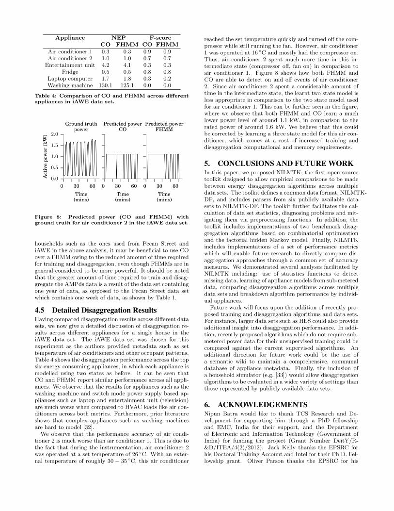
4.5 Detailed Disaggregation ResultsHaving compared disaggregation results across different datasets, we now give a detailed discussion of disaggregation re-sults across different appliances for a single house in theiAWE data set. The iAWE data set was chosen for thisexperiment as the authors provided metadata such as settemperature of air conditioners and other occupant patterns.Table 4 shows the disaggregation performance across the topsix energy consuming appliances, in which each appliance ismodelled using two states as before. It can be seen thatCO and FHMM report similar performance across all appli-ances. We observe that the results for appliances such as thewashing machine and switch mode power supply based ap-pliances such as laptop and entertainment unit (television)are much worse when compared to HVAC loads like air con-ditioners across both metrics. Furthermore, prior literatureshows that complex appliances such as washing machinesare hard to model [32].

We observe that the performance accuracy of air condi-tioner 2 is much worse than air conditioner 1. This is due tothe fact that during the instrumentation, air conditioner 2was operated at a set temperature of 26 ◦C. With an exter-nal temperature of roughly 30 − 35 ◦C, this air conditioner

reached the set temperature quickly and turned off the com-pressor while still running the fan. However, air conditioner1 was operated at 16 ◦C and mostly had the compressor on.Thus, air conditioner 2 spent much more time in this in-termediate state (compressor off, fan on) in comparison toair conditioner 1. Figure 8 shows how both FHMM andCO are able to detect on and off events of air conditioner2. Since air conditioner 2 spent a considerable amount oftime in the intermediate state, the learnt two state model isless appropriate in comparison to the two state model usedfor air conditioner 1. This can be further seen in the figure,where we observe that both FHMM and CO learn a muchlower power level of around 1.1 kW, in comparison to therated power of around 1.6 kW. We believe that this couldbe corrected by learning a three state model for this air con-ditioner, which comes at a cost of increased training anddisaggregation computational and memory requirements.

5. CONCLUSIONS AND FUTURE WORKIn this paper, we proposed NILMTK; the first open sourcetoolkit designed to allow empirical comparisons to be madebetween energy disaggregation algorithms across multipledata sets. The toolkit defines a common data format, NILMTK-DF, and includes parsers from six publicly available datasets to NILMTK-DF. The toolkit further facilitates the cal-culation of data set statistics, diagnosing problems and mit-igating them via preprocessing functions. In addition, thetoolkit includes implementations of two benchmark disag-gregation algorithms based on combinatorial optimisationand the factorial hidden Markov model. Finally, NILMTKincludes implementations of a set of performance metricswhich will enable future research to directly compare dis-aggregation approaches through a common set of accuracymeasures. We demonstrated several analyses facilitated byNILMTK including: use of statistics functions to detectmissing data, learning of appliance models from sub-metereddata, comparing disaggregation algorithms across multipledata sets and breakdown algorithm performance by individ-ual appliances.

Future work will focus upon the addition of recently pro-posed training and disaggregation algorithms and data sets.For instance, larger data sets such as HES could also provideadditional insight into disaggregation performance. In addi-tion, recently proposed algorithms which do not require sub-metered power data for their unsupervised training could becompared against the current supervised algorithms. Anadditional direction for future work could be the use ofa semantic wiki to maintain a comprehensive, communaldatabase of appliance metadata. Finally, the inclusion ofa household simulator (e.g. [33]) would allow disaggregationalgorithms to be evaluated in a wider variety of settings thanthose represented by publicly available data sets.

6. ACKNOWLEDGEMENTSNipun Batra would like to thank TCS Research and De-velopment for supporting him through a PhD fellowshipand EMC, India for their support, and the Departmentof Electronic and Information Technology (Government ofIndia) for funding the project (Grant Number DeitY/R-&D/ITEA/4(2)/2012). Jack Kelly thanks the EPSRC forhis Doctoral Training Account and Intel for their Ph.D. Fel-lowship grant. Oliver Parson thanks the EPSRC for his

Doctoral Prize Award. The authors thank the anonymousreviewers for their feedback, and also Denzil Correa, PhDstudent IIIT Delhi for his valuable comments.

7. REFERENCES[1] G. W. Hart. Nonintrusive appliance load monitoring.

Proceedings of the IEEE, 80(12):1870–1891, 1992.doi:10.1109/5.192069.

[2] S. Darby. The effectiveness of feedback on energyconsumption. A Review for DEFRA of the Literatureon Metering, Billing and direct Displays, 2006.

[3] California Public Utilities Commission. Final OpinionAuthorizing Pacific Gas and Electric Company toDeploy Advanced Metering Infrastructure. Technicalreport, 2006.

[4] Department of Energy & Climate Change. SmartMetering Equipment Technical Specifications Version2. Technical report, UK, 2013.

[5] J. Z. Kolter and M. J. Johnson. REDD: A public dataset for energy disaggregation research. In Proceedingsof 1st KDD Workshop on Data Mining Applications inSustainability, San Diego, CA, USA, 2011.

[6] K. Anderson, A. Ocneanu, D. Benitez, D. Carlson,A. Rowe, and M. Berges. BLUED: A fully labeledpublic dataset for Event-Based Non-Intrusive loadmonitoring research. In Proceedings of 2nd KDDWorkshop on Data Mining Applications inSustainability, pages 12–16, Beijing, China, 2012.

[7] S. Barker, A. Mishra, D. Irwin, E. Cecchet, P. Shenoy,and J. Albrecht. Smart*: An open data set and toolsfor enabling research in sustainable homes. InProceedings of 2nd KDD Workshop on Data MiningApplications in Sustainability, Beijing, China, 2012.

[8] A. L. Goldberger, L. A. Amaral, L. Glass, J. M.Hausdorff, P. C. Ivanov, R. G. Mark, J. E. Mietus,G. B. Moody, C.-K. Peng, and H. E. Stanley.PhysioBank, PhysioToolkit, and PhysioNet:components of a new research resource for complexphysiologic signals. Circulation, 101(23):e215–e220,2000. doi:10.1161/01.cir.101.23.e215.

[9] D. Kotz and T. Henderson. Crawdad: A communityresource for archiving wireless data at dartmouth.Pervasive Computing, IEEE, 4(4):12–14, 2005.doi:10.1109/MPRV.2005.75.

[10] F. Pedregosa, G. Varoquaux, A. Gramfort, V. Michel,B. Thirion, O. Grisel, M. Blondel, P. Prettenhofer,R. Weiss, V. Dubourg, J. Vanderplas, A. Passos,D. Cournapeau, M. Brucher, M. Perrot, andE. Duchesnay. Scikit-learn: Machine learning inPython. Journal of Machine Learning Research,12:2825–2830, 2011. arXiv:1201.0490.

[11] H. Kim, M. Marwah, M. F. Arlitt, G. Lyon, andJ. Han. Unsupervised Disaggregation of LowFrequency Power Measurements. In Proceedings of11th SIAM International Conference on Data Mining,pages 747–758, Mesa, AZ, USA, 2011.doi:10.1137/1.9781611972818.64.

[12] K. C. Armel, A. Gupta, G. Shrimali, and A. Albert. Isdisaggregation the holy grail of energy efficiency? Thecase of electricity. Energy Policy, 52:213–234, 2013.doi:10.1016/j.enpol.2012.08.062.

[13] C. Holcomb. Pecan Street Inc.: A Test-bed for NILM.In International Workshop on Non-Intrusive LoadMonitoring, Pittsburgh, PA, USA, 2012.

[14] J.-P. Zimmermann, M. Evans, J. Griggs, N. King,L. Harding, P. Roberts, and C. Evans. HouseholdElectricity Survey. A study of domestic electricalproduct usage. Technical Report R66141, DEFRA,May 2012.

[15] S. Makonin, F. Popowich, L. Bartram, B. Gill, andI. V. Bajic. AMPds: A Public Dataset for LoadDisaggregation and Eco-Feedback Research. In IEEEElectrical Power and Energy Conference, Halifax, NS,Canada, 2013.

[16] N. Batra, M. Gulati, A. Singh, and M. B. Srivastava.It’s Different: Insights into home energy consumptionin India. In Proceedings of the Fifth ACM Workshopon Embedded Sensing Systems for Energy-Efficiency inBuildings, 2013. doi:10.1145/2528282.2528293.

[17] J. Kelly and W. Knottenbelt. ‘UK-DALE’: A datasetrecording UK Domestic Appliance-Level Electricitydemand and whole-house demand. ArXiv e-prints,2014. arXiv:1404.0284.

[18] J. Z. Kolter and T. Jaakkola. Approximate Inferencein Additive Factorial HMMs with Application toEnergy Disaggregation. In Proceedings of theInternational Conference on Artificial Intelligence andStatistics, pages 1472–1482, La Palma, CanaryIslands, 2012.

[19] M. Zeifman. Disaggregation of home energy displaydata using probabilistic approach. IEEE Transactionson Consumer Electronics, 58(1):23–31, 2012.doi:10.1109/TCE.2012.6170051.

[20] M. J. Johnson and A. S. Willsky. BayesianNonparametric Hidden Semi-Markov Models. Journalof Machine Learning Research, 14:673–701, 2013.arXiv:1203.1365.

[21] O. Parson, S. Ghosh, M. Weal, and A. Rogers.Non-intrusive load monitoring using prior models ofgeneral appliance types. In Proceedings of the 26thAAAI Conference on Artificial Intelligence, pages356–362, Toronto, ON, Canada, 2012.

[22] D. Rahayu, B. Narayanaswamy, S. Krishnaswamy,C. Labbe, and D. P. Seetharam. Learning to beenergy-wise: Discriminative methods for loaddisaggregation. In 3rd International Conference onFuture Energy Systems, pages 1–4, 2012.doi:10.1145/2208828.2208838.

[23] N. Batra, H. Dutta, and A. Singh. INDiC: ImprovedNon-Intrusive load monitoring using load Division andCalibration. In International Conference of MachineLearning and Applications, Miami, FL, USA, 2013.

[24] K. Anderson, M. Berges, A. Ocneanu, D. Benitez, andJ. Moura. Event detection for non intrusive loadmonitoring. In Proceedings of 38th Annual Conferenceon IEEE Industrial Electronics Society, pages3312–3317, 2012. doi:10.1109/IECON.2012.6389367.

[25] Y. Low, J. Gonzalez, A. Kyrola, D. Bickson,C. Guestrin, and J. M. Hellerstein. Graphlab: A newparallel framework for machine learning. InConference on Uncertainty in Artificial Intelligence,Catalina Island, CA, USA, 2010. arXiv:1006.4990.

[26] A. Schoofs, A. Guerrieri, D. T. Delaney, G. O’Hare,and A. G. Ruzzelli. ANNOT: Automated ElectricityData Annotation Using Wireless Sensor Networks. InProceedings of the 7th Annual IEEE CommunicationsSociety Conference on Sensor Mesh and Ad HocCommunications and Networks, Boston, MA, USA,2010. doi:10.1109/SECON.2010.5508248.

[27] J. Kelly and W. Knottenbelt. Metadata for EnergyDisaggregation. ArXiv e-prints, Mar. 2014.arXiv:1403.5946.

[28] Z. Ghahramani and M. I. Jordan. Factorial hiddenmarkov models. Machine learning, 29(2-3):245–273,1997. doi:10.1023/A:1007425814087.

[29] Richard de Dear and Melissa Hart. ApplianceElectricity End-Use: Weather and Climate Sensitivity.Technical report, Sustainable Energy Group,Australian Greenhouse Office, 2002.

[30] A. Kavousian, R. Rajagopal, and M. Fischer.Determinants of residential electricity consumption:Using smart meter data to examine the effect ofclimate, building characteristics, appliance stock, andoccupants’ behavior. Energy, 55(0):184 – 194, 2013.doi:10.1016/j.energy.2013.03.086.

[31] M. Wytock and J. Zico Kolter. ContextuallySupervised Source Separation with Application toEnergy Disaggregation. ArXiv e-prints, 2013.arXiv:1312.5023.

[32] S. Barker, S. Kalra, D. Irwin, and P. Shenoy.Empirical characterization and modeling of electricalloads in smart homes. In IEEE International GreenComputing Conference, pages 1–10, Arlington, VA,USA, 2013. doi:10.1109/IGCC.2013.6604512.

[33] J. Liang, S. K. K. Ng, G. Kendall, and J. W. M.Cheng. Load Signature Study - Part II: DisaggregationFramework, Simulation, and Applications. IEEETransactions on Power Delivery, 25(2):561–569, 2010.doi:10.1109/TPWRD.2009.2033800.

APPENDIXA. SAMPLE CODE FOR NILMTK PIPELINEAlgorithm 1 illustrates the NILMTK pipeline via a minimalcode example.

Algorithm 1 Example code of complete pipeline.

dataset = DataSet()

# Load the dataset

dataset.load_hdf5(DATASET_PATH)

# Load first house

building = dataset.buildings[1]

# Remove records where voltage<160

building = filter_out_implausible_values(

building, Measurement(‘voltage’, ‘’), 160)

# Downsample to 1 minute

building = downsample(building, rule=‘1T’)

# Choosing feature for disaggregation

DISAGG_FEATURE = Measurement(‘power’, ‘active’)

# Dividing the data into train and test

train, test = train_test_split(building)

# Train on DISAGG_FEATURES using FHMM

disaggregator = FHMM()

disaggregator.train(train, disagg_features=

[DISAGG_FEATURE])

# Disaggregate

disaggregator.disaggregate(test)

# F1 score metric

f1_score = f1(disaggregator.predictions,

test)

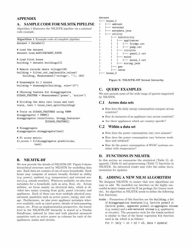
B. NILMTK-DFWe now provide the details of NILMTK-DF. Figure 9 showshierarchical structure used by NILMTK for modelling datasets. Each data set consists of one of more households. Eachhouse may comprise of sensors broadly divided as utility(e.g. power), ambient (e.g. temperature) and external sen-sors (e.g. outside weather). Wherever available, we also storemetadata for a household, such as area, floor, etc. Acrossutilities, we focus mainly on electrical data, which is di-vided into mains (coming from grid), panel (circuits) andappliances. Each of these can store multiple physical mea-surement quantities such as active power, energy and volt-age. Furthermore, we also store appliance metadata wher-ever available, such as rated power, details of instrumentingsensor, etc. From an implementation perspective, the lowestlevel in the NILMTK-DF hierarchy is stored as a PandasDataFrame, indexed by time and with physical measuredquantities such as active power as columns for each of theappliances, mains and circuits.

dataset

|--- house_1

| |--- ambient

| |--- external

| |--- metadata.json

| |--- utility

| |--- electricity

| | |--- appliances

| | | |--- fridge.csv

| | | |--- pump.csv

| | |--- circuits

| | | |--- panel_1.csv

| | |--- mains

| | | |--- mains_1.csv

| | |--- wiring.json

| |--- gas

| |--- water

|--- house_2

Figure 9: NILMTK-DF format hierarchy

C. QUERY EXAMPLESWe now present some of the wide range of queries supportedby NILMTK.

C.1 Across data sets• How does the daily energy consumption compare across

countries?

• How do instances of an appliance vary across countries?

• Are there appliances which are country specific?

C.2 Within a data set• How does the power consumption vary over seasons?

• How does the power consumption vary between week-days and weekend?

• How do the power consumption of HVAC systems cor-relate with temperature?

D. FUNCTIONS IN NILMTKIn this section we summarise the statistical (Table 5), di-agnostic (Table 6) and preprocessing (Table 7) functions inNILMTK. An interested reader may refer the online docu-mentation for updates.

E. ADDING A NEW NILM ALGORITHMWe designed NILMTK to ensure that new algorithms areeasy to add. We modelled our interface on the highly suc-cessful scikit-learn and the R lm package (for Linear mod-els). An algorithm in NILMTK needs to define the followingfour functions:

train : Parameters of this function are the building, a listof disaggregation features (e.g. [active power] or[active power, apparent power], an aggregate stream

(e.g. mains) and a sub-metered stream (e.g. appliancesor circuits). The parameter style for the train methodis similar to that of the linear regression fit functionused in lm, which is as follows:

fit <- lm(y ∼ x1 + x2 + x3, data = mydata)

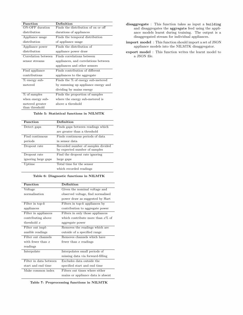
Function DefinitionON-OFF duration Finds the distribution of on or off

distribution durations of appliances

Appliance usage Finds the temporal distribution

distribution of appliance usage

Appliance power Finds the distribution of

distribution appliance power draw

Correlation between Finds correlations between

sensor streams appliances, and correlations between

appliances and other sensors

Find appliance Finds contribution of different

contributions appliances to the aggregate

% energy sub- Finds the % of energy sub-metered

metered by summing up appliance energy and

dividing by mains energy

% of samples Finds the proportion of samples

when energy sub- where the energy sub-metered is

metered greater above a thresholdthan threshold

Table 5: Statistical functions in NILMTK

Function Definition

Detect gaps Finds gaps between readings which

are greater than a threshold

Find continuous Finds continuous periods of data

periods in sensor data

Dropout rate Recorded number of samples dividedby expected number of samples

Dropout rate Find the dropout rate ignoring

ignoring large gaps large gaps

Uptime Total time for the sensor

which recorded readings

Table 6: Diagnostic functions in NILMTK

Function Definition

Voltage Given the nominal voltage and

normalisation observed voltage, find normalised

power draw as suggested by Hart

Filter in top-k Filters in top-k appliances by

appliances contribution to aggregate power

Filter in appliances Filters in only those appliances

contributing above which contribute more than x% of

threshold x aggregate power

Filter out impl- Removes the readings which are

ausible readings outside of a specified range

Filter out channels Removes channels which have

with fewer than x fewer than x readings

readings

Interpolate Interpolates small periods of

missing data via forward-filling

Filter in data between Excludes data outside the

start and end time specified start and end time

Make common index Filters out times where either

mains or appliance data is absent

Table 7: Preprocessing functions in NILMTK

disaggregate : This function takes as input a building

and disaggregates the aggregate feed using the appli-ance models learnt during training. The output is adisaggregated stream for individual appliances.

import model : This function should import a set of JSONappliance models into the NILMTK disaggregator.

export model : This function writes the learnt model toa JSON file.