nmrpipe · nmrpipe: spectral processing as a unix pipeline . 1d-4d ft, lp, mem, ml, pca . parallel...
TRANSCRIPT
Page 1
July 2012 Frank Delaglio
ΣΠΑΡΤΑ+

Spectrometer Format Conversion
1D-4D Fourier Transform and Signal Enhancement
Spectral Visualization
1D-4D Peak Detection and Quantification: Position, Amplitude, Width and Modulation/Evolution
Spectral Assignment
Extraction of Structural Parameters
Molecular Structure Calculation
Molecular Display and Structure Verification
Exploitation of Structure
Spectral Imaging
Automation, Batch Analysis, and Screening
Web-Based Server Implementations
July 2012 [email protected]
Ad Bax ● Joeseph Barchi ● James Chou ● Gabriel Cornilescu ● George Gray ● Alex Grishaev Stephan Grzesiek ● Georg Kontaxis ● John Kuszewski ● Ryan McKay ● John Pfeiffer
Ben Ramirez ● Michael Shapiro ● Tobias Ulmer ● Gerteen Vuister ● Justin Wu ● Jinfa Ying Shen Yang ● Guang Zhu ● Edward Zartler
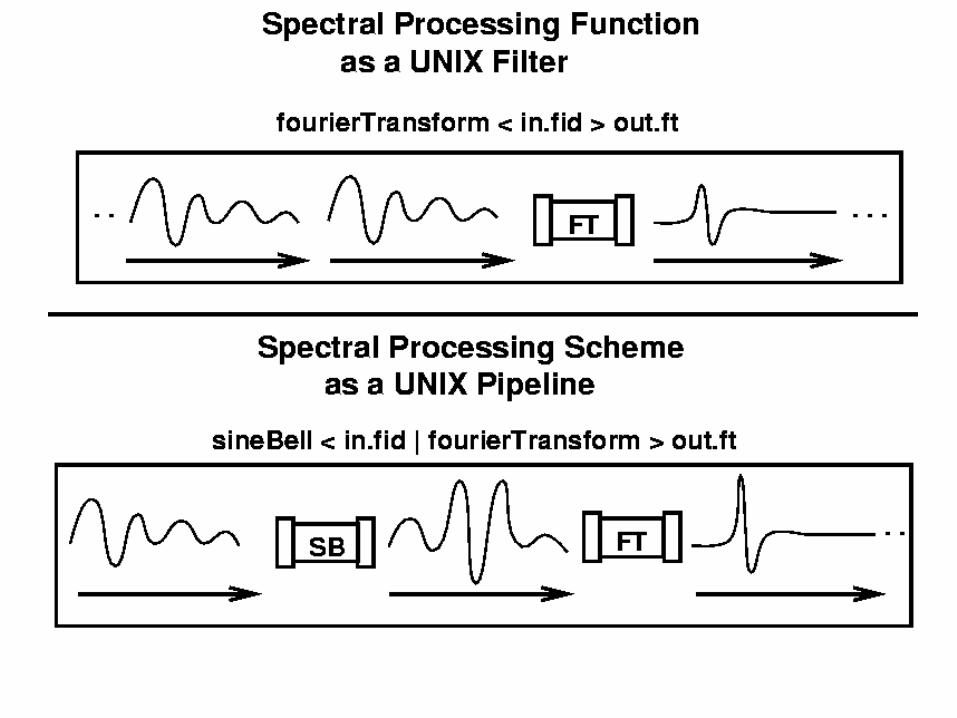

NMRPipe: Spectral Processing as a UNIX Pipeline
1D-4D FT, LP, MEM, ML, PCA Parallel Processing 1D-4D Peak Detection and Quantification Spectral Graphics, Strips, Projections Extensively Customizable Molecular Structure Calculation
NMR Parameter Calculation (Shifts, Dipolar Couplings, PCS, etc) Customization is via standard scripting languages (C-shell, TCL) Created and Maintained by one developer, with contributed modules Solaris, IRIX, HP/UX, DEC OSF, IBM AIX, IBM Blue Gene, Convex OS, Cray OS, Mac OS X, Linux, WindowsXP Interix, VMWare Player Bottom-up Software Design


NMRWish
Customized version of TCL/TK “wish” interpreter Script-based Interactive Spectral graphics (multi-window and PostScript) Generic Database Engine (GDB) Manipulate Peak Data, Assignments, NMR Parameters, and Molecular Structure


Analyze Titration Curve to Estimate Kd


Bax Group NMR Calculation Servers http://spin.niddk.nih.gov/bax/nmrserver

ΣΠΑΡΤΑ+
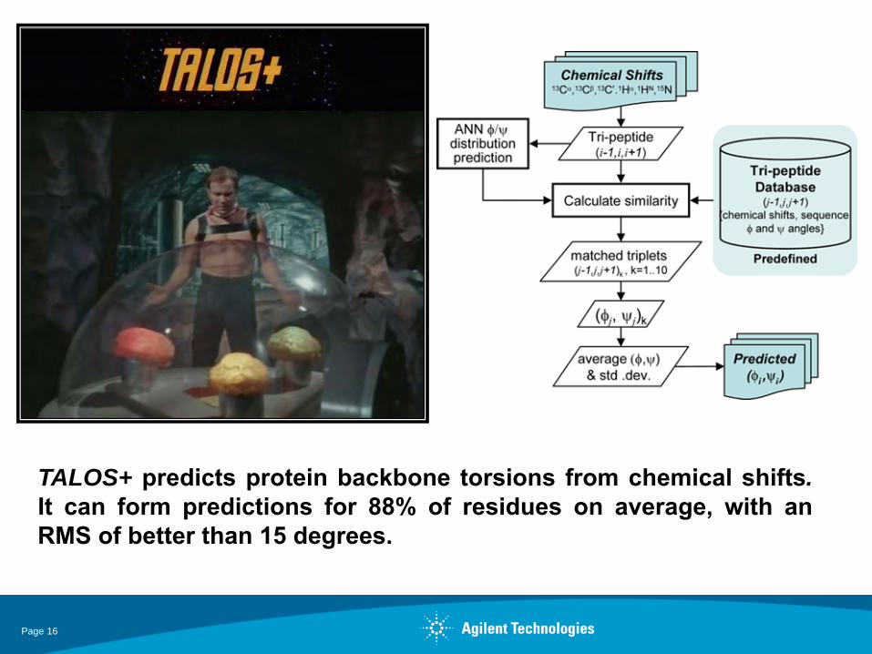
TALOS+: prediction of protein backbone phi,psi torsions From chemical shifts.
SPARTA+: prediction of protein backbone chemical shifts from structure.
PROMEGA: prediction of PRO cis-trans conformation from backbone chemical shifts.
DYNAMO/PDBUTIL: simple structure calcuation, utilities to add protons, create extended structures, etc.
DC: manipulation of Dipolar Couplings and NMR Homology Search (MFR).
AXES: prediction of Small-Angle X-Ray Scattering from PDB
NMRPipe: Related Programs and Features
Page 16
TALOS+ predicts protein backbone torsions from chemical shifts. It can form predictions for 88% of residues on average, with an RMS of better than 15 degrees.

Page 17

Page 18
ΣΠΑΡΤΑ+


• Rotate PDB onto Tensor Frame
• Molecular Fragment Replacement
• Amino Acid Type by Chemical Shift
Tensor and NMR Homology Search Utilities

Page 21
• Create Extended Structure
• Add Protons
• Transformations of PDB Coordinates
• List Secondary Structure, H-Bonds
• Mass, Volume, Surface Area
• Simple simulated annealing

Page 22

Page 23

Page 24
Manually Select Acquisition Mode
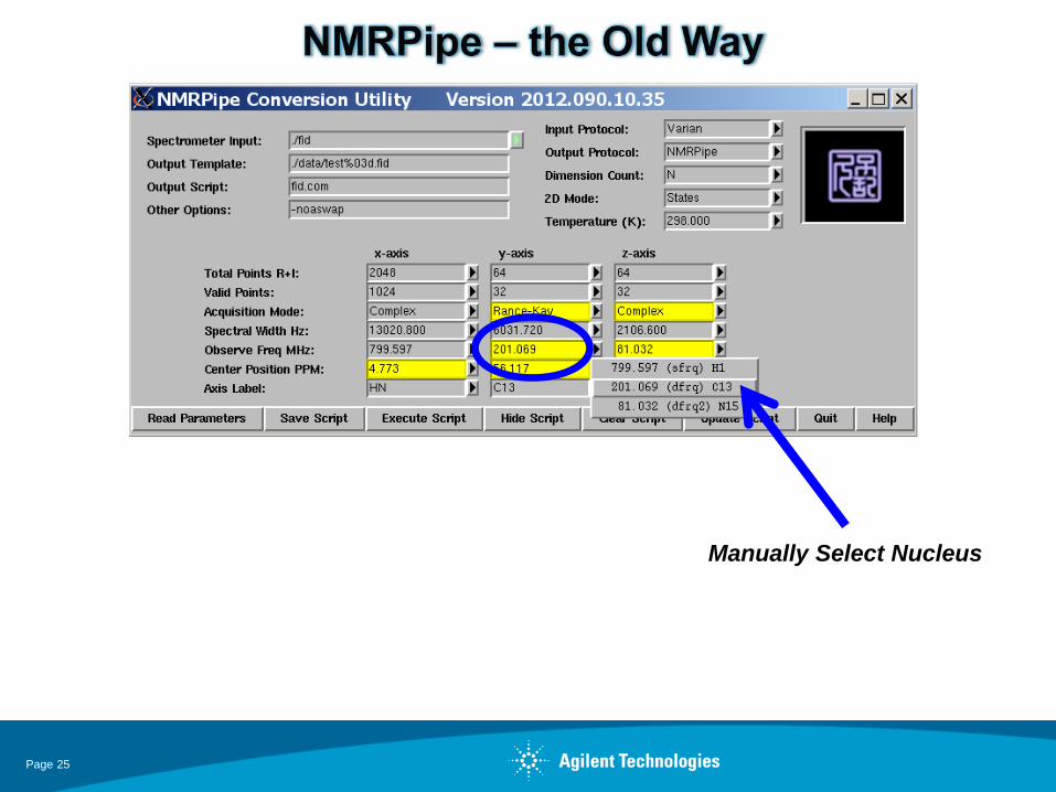
Page 25
Manually Select Nucleus

Page 26
Manually Select Axis Label

Page 27
Traditionally, NMRPipe scripts are manually edited to set parameter values
#!/bin/csh
xyz2pipe -in fid/test%03d.fid -x -verb \ | nmrPipe -fn SOL \ | nmrPipe -fn SP -off 0.5 -end 0.98 -pow 2 -c 0.5 \ | nmrPipe -fn ZF \ | nmrPipe -fn FT \ | nmrPipe -fn PS -p0 43.0 -p1 0.0 -di \ | nmrPipe -fn EXT –x1 10.5ppm –xn 5.7ppm -sw \ | nmrPipe -fn TP \ | nmrPipe -fn SP -off 0.5 -end 0.98 -pow 1 -c 1.0 \ | nmrPipe -fn ZF \ | nmrPipe -fn FT \ | nmrPipe -fn PS -p0 -90.0 -p1 180.0 -di \ | nmrPipe -fn TP \ | nmrPipe -fn POLY -auto \ | pipe2xyz -out ft/test%03d.ft2 -x -to 0 xyz2pipe -in ft/test%03d.ft2 -z -verb \ | nmrPipe -fn SP -off 0.5 -end 0.98 -pow 1 -c 0.5 \ | nmrPipe -fn ZF \ | nmrPipe -fn FT \ | nmrPipe -fn PS -p0 0.0 -p1 0.0 -di \ | pipe2xyz -out ft/test%03d.ft3 -z

Page 28
Now, values determined in VnmrJ can be automatically inserted into any NMRPipe script
#!/bin/csh
xyz2pipe -in _inName_ -x -verb \ | nmrPipe -fn SOL \ | nmrPipe -fn SP -off 0.5 -end 0.98 -pow 2 -c _xC1_ \ | nmrPipe -fn ZF \ | nmrPipe -fn FT \ | nmrPipe -fn PS -p0 _xP0_ -p1 _xP1_ -di \ | nmrPipe -fn EXT –x1 _xEXTX1_ –xn _xEXTXN_ -sw \ | nmrPipe -fn TP \ | nmrPipe -fn SP -off 0.5 -end 0.98 -pow 1 -c _yC1_ \ | nmrPipe -fn ZF \ | nmrPipe -fn FT \ | nmrPipe -fn PS -p0 _yP0_ -p1 _yP1_ -di \ | nmrPipe -fn TP \ | nmrPipe -fn POLY -auto \ | pipe2xyz -out _auxName_ -x -to 0 xyz2pipe -in _auxName_ -z -verb \ | nmrPipe -fn SP -off 0.5 -end 0.98 -pow 1 -c _zC1_ \ | nmrPipe -fn ZF \ | nmrPipe -fn FT \ | nmrPipe -fn PS -p0 _zP0_ -p1 _zP1_ -di \ | pipe2xyz -out _outName_ -z

Page 29
Automatically Create and Run NMRPipe Scripts

Page 30
The VnmrJ “Do it All” Button

Page 31
Strip display overview of processed result is created automatically

Page 32
Strip display schemes for multiple spectra can be created automatically

Page 33
CBCA(CO)NH NUS Sampling Schedule
25% Density
Original Data ¼ Resolution NUS
13C (10% Decay)
15N (U
niform)
FT LP ML MEM FT LP ML MEM FT ML MEM

Page 34

Page 35

x ix
1 i
2 -1
3 -i
4 1
5 i
6 -1
7 -i
8 1

x ix
1 i
2 -1
3 -i
4 1
5 i
6 -1
7 -i
8 1
exp( -i 2πft ) = cos( 2πft ) - i sin( 2πft ) … exp( i 2πft ) = cos( 2πft ) + i sin( 2πft )


Page 40
X( f ) = Σ x( t ) [ cos( 2πft / N ) - i sin( 2πft / N ) ]
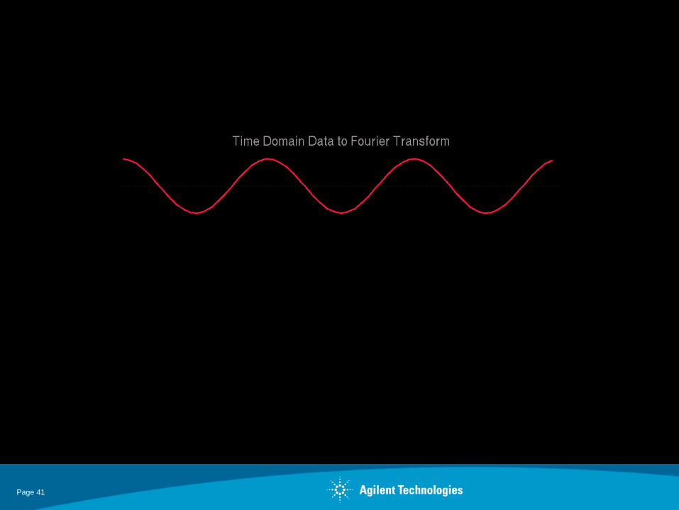
Page 41

Page 42

/* Fourier transform of complex data tR,tI to produce fR,fI. */
void ft( float *tR, float *tI, float *fR, float *fI, int size ) { float vR, vI, twoPI; int mid, k, n; twoPI = 4.0*acos( 0.0 ); mid = size/2; for( k = 0; k < size; k++ ) /* For every output freq point … */ { fR[k] = 0.0; fI[k] = 0.0; for( n = 0; n < size; n++ ) /* Sum over input times sinusoid. */ { f = twoPI*(k - mid)*n/size; vR = cos( f ); vI = sin( f ); fR[k] += tR[n]*vR - tI[n]*vI; fI[k] += tR[n]*vI + tI[n]*vR; } } }

Page 44

Page 45

Page 46

Page 47


exp( -i 2πft ) = cos( 2πft ) - i sin( 2πft )

exp( -i 2πft ) = cos( 2πft ) - i sin( 2πft )

exp( -i 2πft ) = cos( 2πft ) - i sin( 2πft )

Page 55

Linear Prediction


Page 58

xyz2pipe -in fid/test%03d.fid -x -verb \ # Process the Directly-detected X-Axis. | nmrPipe -fn SOL \ | nmrPipe -fn SP -off 0.5 -end 0.98 -pow 2 -c 0.5 \ | nmrPipe -fn ZF -auto \ | nmrPipe -fn FT \ | nmrPipe -fn PS -p0 43 -p1 0.0 -di \ | nmrPipe -fn EXT -x1 11.5ppm -xn 5.5ppm -sw \ | pipe2xyz -out lp/x%03d.ft1 -x xyz2pipe -in lp/x%03d.ft1 -z -verb \ # Process the Indirectly-detected Z-Axis. | nmrPipe -fn SP -off 0.5 -end 0.95 -pow 1 -c 0.5 \ | nmrPipe -fn ZF -auto \ | nmrPipe -fn FT \ | nmrPipe -fn PS -p0 0.0 -p1 0.0 -di \ | pipe2xyz -out lp/xz%03d.ft2 -z xyz2pipe -in lp/xz%03d.ft2 -y -verb \ # Linear Predict and Process the | nmrPipe -fn LP -fb -ord 12 \ # Indirectly-Detected Z-Axis. | nmrPipe -fn SP -off 0.5 -end 0.98 -pow 1 -c 1.0 \ | nmrPipe -fn ZF -auto \ | nmrPipe -fn FT \ | nmrPipe -fn PS -p0 -135 -p1 180 -di \ | pipe2xyz -out lp/xyz%03d.ft3 -y xyz2pipe -in lp/xyz%03d.ft3 -z -verb \ # Inverse Process, Linear Predict, | nmrPipe -fn HT -auto \ # and Re-Process the Z-Axis | nmrPipe -fn PS -inv -hdr \ | nmrPipe -fn FT -inv \ | nmrPipe -fn ZF -inv \ | nmrPipe -fn SP -inv -hdr \ | nmrPipe -fn LP -fb \ | nmrPipe -fn SP -off 0.5 -end 0.98 -pow 1 -c 0.5 \ | nmrPipe -fn ZF -auto \ | nmrPipe -fn FT \ | nmrPipe -fn PS -hdr -di \ | pipe2xyz -out lp/test%03d.ft3 -z

FT FT with LP Linear Prediction

Page 61
Non-Uniform Sampling on a Uniform Grid

Page 62
Non-Uniform Sampling: Skip a Fraction of the Points

Page 63
Non-Uniform Sampling

Page 64
Non-Uniform Sampling: for Fourier Transform, Replace Missing Points with Zeros

Page 65

Page 66

Page 67

Page 68

Page 69

Page 70

Page 71
Maximum Entropy Methods

Page 72
Maximum Entropy Methods

Page 73

Page 74
Threshold Methods

Page 75
Threshold Methods

Maximum Entropy Method

Page 77
( A )
( B )
( B – c A )
( scale c = ) A B
A A ___ Σ

Page 78
( A )
( B )
( B – c A )
( scale c = ) A B
A A ___ Σ

Page 79

Page 80
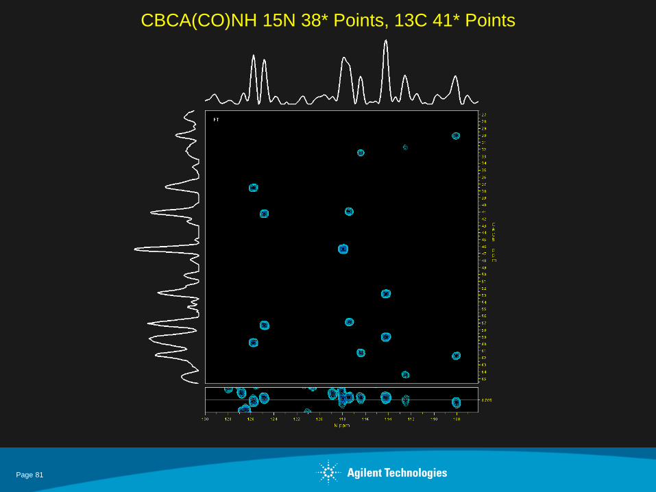
CBCA(CO)NH NUS Sampling Schedule
25% Density
Original Data ¼ Resolution NUS
13C (10% Decay)
15N (U
niform)
FT LP ML MEM FT LP ML MEM FT ML MEM
Page 81
CBCA(CO)NH 15N 38* Points, 13C 41* Points

Page 82
FT
LP ML MEM
FT 1/4 FT NUS

Page 83
FT
LP 1/4 ML NUS MEM NUS
FT 1/4 FT NUS

Page 84
Linearity – Reconstructed Peak Height vs Peak Height in FT Spectrum
ML MEM

Page 85

Page 86
Matrix Decomposition: Each Multidimensional NMR Signal is the Product of 1D Vectors
+ =
= =

Page 87
X X
NUS – Missing Information in a Deleted Point is Also Contained in the Same Row or Column

Page 88
Spectral Matrix Decomposition by Principal Component Analysis (PCA)
Page 88

Page 89
Spectral Matrix Decomposition by Principal Component Analysis (PCA)
+ =

Page 90

Page 91

Page 92

Page 93

Page 94

Page 95

Page 96

Page 97

Page 98

Page 99


Page 101

Chemical Shift
J-Coupling
NOE Distance
Structural Data from NMR

Identify many H-H short range NOE distances
Supplement with torsions from J-Coupling values
Assume standard peptide geometry
Use simulated annealing to find a structure which matches distances

NOE distances are only qualitative
A given peak might be the only evidence of an interaction
A mis-assigned peak can be similarly problematic


Alternate Approaches to NMR Structure Chemical Shifts


Use chemical shifts directly rather than secondary shifts (SS).
For a given residue in the target:
For a given residue type in the database:
Compute chemical shift distance.
Use Gaussian to estimate a P value
Find avg P value for residue type
Normalize over all residue types
Residue Type Probability from Chemical Shifts
DINI SS Method D81 Residues
50 14 4 2 3 (8)
61.7% 17.3% 4.9% 2.4% 3.7% 9.9%
DINI Direct Method 81 Residues:
64 11 3 2 1 0
79.0% 13.6% 3.7% 2.5% 1.2% 0%
FBP 170 residues:
129 20 10 6 2 (3)
75.9% 11.8% 5.9% 3.5% 1.2% (1.8%)
V-Alpha 114 residues:
66 18 14 2 3 (11)
57.9% 15.8% 12.3% 1.8% 2.6% (9.6%)
Gamma Crystalin 170 residues:
87 24 20 12 8 (19)
51.2% 14.1% 11.8% 7.1% 4.7% 11.2%

Subtract Residue-Specific Random Coil Shift to form Secondary Shift


Chemical Shift and Backbone Structure Motif
Match database triplet with target, based on sum-of squares difference in chemical shifts, plus residue type homology term.
Use central residue as predictor of phi and psi.


The SPARTA Program of Shen and Bax …

Alternate Approaches to NMR Structure Residual Dipolar Couplings
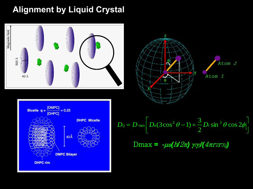
Alignment by Liquid Crystal
+−= φθθ 2cossin
23)1cos3( 22
max raij DDDD
Dmax = -µ0(h/2π) γiγj/(4πr2r3ij)

isotropic 5% w/v bicelles 8% w/v bicelles
1H-15N HSQC spectra of ubiquitin
Alignment: 0 % 0.1% 0.16%


+−= φθθ 2cossin
23)1cos3( 22
max raij DDDD
Dab = Dmax [ (s1)*0.5*(3.0*zIJ*zIJ - 1.0)
+ (s2)*0.5*(xIJ*xIJ - yIJ*yIJ)
+ (s3)*2.0*xIJ*yIJ
+ (s4)*2.0*xIJ*zIJ
+ (s5)*2.0*yIJ*zIJ ]


• Search PDB for small fragments whose simulated dipolar couplings and shifts match the observed values.
• Use the fragment information to reconstitute larger structural elements.
• Also: Sequential NOEs, J values, etc. • Nucleic Acid Applications
Molecular Fragment Replacement (MFR)

Initial Structure from Average Phi and Psi of Fragment
Ensemble
1ubq vs MFR phi/psi refined structure

MFR Estimation of Tensor Parameters
• Magnitude
• Rhombicity
• Orientation (Euler Angles)

MFR Fragment Tensor Magnitudes Reveal Dynamics
S42

Gamma S
177 Residues, two similar domains, homologous structure is known.
179 Amide-Amide NOEs, 70 Methyl-Methyl NOEs, including 6 inter-domain
DC Medium 1: 144 HN-N, 111 CA-CB, 150 CA-C’, 134 N-C’
DC Medium 2: 147 HN-N, 135 CA-CB, 153 CA-C’, 139 N-C’
Side-chain χ1 angles from 3JNCγ and 3JC′Cγ couplings, χ2 from 3JCγCδ

• Conduct MFR Search with SVD (free tensor) • Conduct second MFR Search with fixed tensor
Da, Rh, and relative orientation • Refine all fragments with fixed tensor Da, Rh to
yield Phi and Psi for 90% of residues; 50% have better than 5 degree RMS consenus; 33% are 3 degree RMS or better.

dynReadGMC -gmc $gmcDir -pdb $pdbName for {set i 1} {$i <= $count} {incr i} \ { dynSimulateAnnealing -graph -print 50 -rasmol 500 \ -sa stepCount init 100 \ stepCount high 24000 \ stepCount cool 8000 \ timeStep all 3 \ temperature all 4000 \ temperature coolEnd 0 \ -fc dc coolEnd 2.0 \ torsion all 50 \ torsion coolEnd 10 \ noe all 25 \ noe coolEnd 100 \ radGyr all 0.0 set outName [format $outTemplate $i] dynWrite -pdb -src $dynInfo(gmc,pdb) -out $outName –rem $dynInfo(energyText) dynRead -pdb -src $dynInfo(gmc,pdb) -in $pdbName incr iseed 111 srand $iseed }
• MFR Torsions Preserve Secondary Structure During High Temperature Phase • During Cooling, MFR Torsion Restraint Force Constant is Decreased • DC Force Constant is Increased as Ideal Fold is Approached

Backbone RMSD γS(NMR) and γB-crystallin (X-ray) C-terminal domain: 1.09 A N-terminal domain: 0.63 A

Consistent blind protein structure generation from NMR chemical shift data Proc Natl Acad Sci USA, (2008) 105, 4685-4690
Yang Shen Oliver Lange Frank Delaglio Paolo Rossi James M. Aramini Gaohua Liu Alexander Eletsky Yibing Wu Kiran K. Singarapu Alexander Lemak Alexandr Ignatchenko Cheryl H. Arrowsmith Thomas Szyperski Gaetano T. Montelione David Baker Ad Bax

Using SPARTA Chemical Shift Prediction to Improve ROSETTA Scoring Function


Protein Number of Residues PDB ID
RMSD Å (backbone)
RMSD Å (all)
% NOE Peak
Agreement
RpT7 65 2jtv 0.64 1.29 69
StR82 69 2jt1 0.57 1.14 65
RhR95 72 2jvm 0.66 1.18 55
NeT4 73 2jv8 0.70 1.42 57
TR80 78 2jxt 0.69 1.27 67
VfR117 80 2jvw 0.60 1.40 37
PsR211 100 2jva 2.07 2.34 57
AtR23 101 2jya 1.10 1.81 60
NeR45A 147 2jxn 2.03 2.85 53
CS-ROSETTA performance on nine structural genomics proteins
StR82
PsR211
NeR45A


Structures of two designed proteins with high sequence identity
NMR structures of Ga88 and Gb88 NMR structures vs csRosetta models
1.07A Mean-to-mean backbone RMSD
1.31A Patrick A. Alexander, Yanan He, Yihong Chen, John Orban, and Philip N. Bryan
PNAS, 2007, 104:11963-11968
PNAS, 2008, 105:14412-14417

NMR Applications in Drug Discovery


NMR Spectral Series: Two Approaches
Applications of NMR in the Drug Discovery Process
SAR by NMR (Abbott Labs)
Observe Ligand Signals
Observe Protein Signals


Amide-HN Chemical Shift of Residue i Am
ide-
N C
hem
ical
Shi
ft of
Res
idue
i


Analyze Titration Curve to Estimate Kd

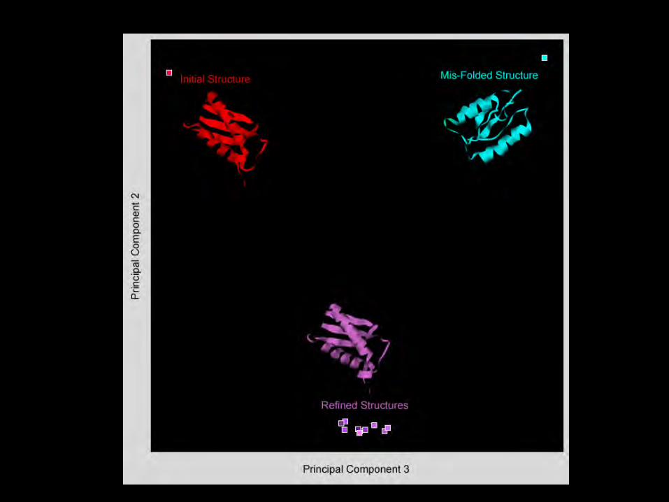
Entire spectrum is a single object in multdimensional space.
Coordinates of the object are the spectral intensities.
Similar spectra cluster together.
Spectra with similar features lie along lines and curves
Multivariate Navigation by Principal Component Analysis (PCA)


Useful Graphics Strategies

Graphics Strategies of Edward Tufte www.edwardtufte.com
Above all, Show the Data
Show Cause and Effect
Represent Data and Scale Faithfully
Maximize “Data Ink” and Data Density, Minimize “Chart Junk”
Shrink Graphics - Integrate Text, Values, and Graphics
Be Multivariate
Use Layers – Use Macro and Micro Interpretations - Clarify by Adding Detail
Conserve Color Space
Use Small Multiples
Find Ways to Show All of the Data
Treat Design as a Solved Problem, then Find the Best Examples

Page 166
Agilent Restricted
Adobe Photoshop “redefines digital imaging with powerful new photography tools and breakthrough capabilities for complex image selections, realistic painting, and intelligent retouching.” - from adobe.com
Microsoft PowerPoint “with new and improved tools for video and photo editing, dramatic new transitions, and realistic animation, you can add polish to presentations that will captivate your audience.” - from microsoft.com
In the content-creation arena, amazon.com lists Microsoft Office and Adobe Photoshop as highest-sellers. It could be claimed, Photoshop is about the content, while PowerPoint is often about the scaffold …

Page 167
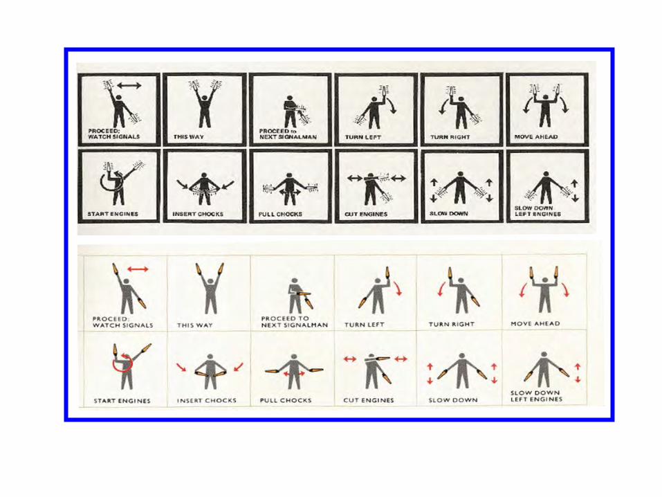
Graphic Design and PowerPoint Abuse: ordered and unordered lists
Agilent Restricted
We rely on PowerPoint to communicate. But there are many enticements to abuse PowerPoint. Beautiful 3D graphics can be used to decorate a presentation and help unify its contents. But in some cases, presentation graphics are used to hide lack of content, or in the worst case, to disguise or misrepresent data. The presentation graphics themselves often have no actual relation to the information being conveyed – they are just ways of dressing up a list or a sequence.
Its useful for us to be able to detect this sort of problem when we see it, avoid this in our own presentations, and avoid it in the User Interface design of our software.
“Impress your audience with these professional and pre-designed 3D PowerPoint Graphics” - from presentationload.com

Page 168
Avoiding inappropriate presentation modes and unneeded 3D effects
Agilent Restricted
Microsoft PowerPoint – “as you can see, the blue-greenish quarter was about the same as the blue one.”
There are no numbers given, and the trend over time, which shows falling sales, is hidden. Also, the 3D perspective might actually distort the apparent values:
Apple Keynote – “as you can see, our maple year was only 1% different than our teak year.”
The segments are at least nicely labeled with numbers, but the wood textures, while really cool, are impossible to decipher. Likewise, the trend with time is hidden, and 3D perspective potentially distorts the apparent values.
The wrong graphical paradigm can make data hard to interpret, or even misleading.
61%
22%
9% 8%
Q1 Q2 Q3 Q4
Quarterly Sales as a Percent of Year Totals
Estimated by Eye from Obscure 3D Pie Chart

Morton Thiokol engineers debated the problem of O-ring failure due to low temperature for several hours the night before the launch, and made the company’s only no-launch request in 12 years. Their presentation of evidence did not convince NASA management. The shuttle blew up 73 seconds after ignition.
Debate on the Challenger Launch


Napolean’s Route: 422,000 Men to 10,000 Men, Five Dimensions


Bax Group Figure: 18 values

Weather Statistics: 1,800+ Values, Four Variables, Notations
.


Page 188