- Bogotá - Colombia - Bogotá - Colombia - Bogotá - Colombia - Bogotá - Colombia - Bogotá - Colombia - Bogotá - Colombia - Bogotá - Colombia - Bogotá - Colombia - B

Okun´s law in Colombia: a non-linear cointegration

By: Luz A. Flórez, Karen L. Pulido-Mahecha, Mario A. Ramos-Veloza

No. 10392018

0

OKUN´S LAW IN COLOMBIA: A NON-LINEAR COINTEGRATION

APPROACH

Luz A. Flórez Karen L. Pulido-Mahecha Mario A. Ramos-Veloza*

Banco de la República -

Medellín

Universidad Nacional Banco de la República-

Bogota

The opinions contained in this document are the sole responsibility of the authors and do not commit

Banco de la República or its Board of Directors.

Abstract

This paper identifies Okun´s law in Colombia between 1984 and 2016 using a

Vector Error Correction Model (VECM) as there is evidence of a long-term

relationship between the unemployment rate and the GDP. Results suggest that

after a one percent increase in GDP, the unemployment rate is reduced by 0.45

percentage points in the long run (after sixteen quarters). In addition we inspect

for nonlinearities using a threshold cointegration model (TVECM). Results

suggest the existence of two regimes a low and a high one. The high regime starts

at the late nineties and is associated with a more flexible labor market. Under

this regime, a 1% increase in GDP, reduces the UR 0.6 percentage points after

eighteen quarters. By contrast, under the low regime the response is 0.2

percentage points after eight quarters.

JEL classification: E24, J3, J4

Keywords: Okun´s law, co-integration, nonlinearities.

* We acknowledge the comments of Luis Fernando Melo and the assistants of the VII Internal research workshop of

the Central Bank and the excellent research assistance of Jose Lobo and Julian Londoño, the authors are the only

responsible of any remaining errors. The authors are researcher Luz Adriana Florez (lflorefl@banrep.gov.co), junior

researcher Mario Ramos (mramosve@banrep.gov.co) and research assistance Kalen Pulido from National University.

1

1. INTRODUCTION

Okun´s law is an empirical regularity that shows the association between unemployment rate and

economic growth. It is named after Arthur Okun (1962) who suggested that a one-percentage point

increase in the unemployment rate is associated with a three-percentage points (pp) fall in the US

output. Further research showed that Okun’s Law also held in other industrialized countries but

with a different magnitude to that estimated for the US. For instance, in France and Germany the

impact was lower given the lower flexibility of their labor markets. Understanding Okun’s Law

does not require a great deal of economic knowledge, which makes it attractive and very useful for

non-specialized audiences, it also has proved to be a power and useful for forecasting [Mitchell and

Pearce (2010)].

Originally Okun proposed two specifications: the difference and the GAP specifications. While in

the difference specification the contemporaneous correlation between the change in unemployment

and economic growth is inspected, in the gap specification the cyclical relationship is inspected.

The cyclical component is computed by removing the permanent component from the series. Thus,

both the differentiation and the subtraction of the long-run trend eliminate any low frequency

movements. The OLS estimates (called the Okun’s Law coefficient (OLC)) capture the short-run

relationship. No specification is inherently superior/preferable given that both have their

drawbacks. While the difference specification does not capture structural changes the gap

specification requires the knowledge of the potential GDP and the natural unemployment rate,

which are unobservable variables [Knotek (2007)].

Vector Autoregressive models (VAR) have also been used to study Okun´s relationship given that

past levels of output may affect current unemployment dynamics, allowing for flexibility in the

timing of the response then the whole effect is not forced to take place immediately. However, this

poses a problem as the interpretation is not straightforward as in the static specification.1 Following

this dynamic analysis, researchers have included the possibility of cointegration among the

variables; that is the existence of a stable long-run relationship between output and unemployment.

Under these conditions a VEC model would better predict the response of output to a drop in

employment than a VAR model [Attfield & Silverstone (1997), Lee(2000)]. Lee (2000) provides

evidence that Okun´s law holds between 1995 and 1996 in 16 OECD countries with remarkable

differences in the estimates across countries. His analysis also considers that the short-run response

can be affected by the long term relationship of these variables and the existence of asymmetries.

1 Another approach to estimate Okun´s Law is to provide an underlying production function that describes the

relationship between output and employment. Using a particular production function, it is possible to account for all

components that determine total output. Thus, output is derived from employment, capital and technology and the

evolution of the output is determined by job creation and total factor productivity (TFP) (e.g. Luchetta and Paradiso

(2014)).

2

He also shows that the “Gap specification” estimates are very sensitive to the detrending

methodology selected.

A more recent question is whether the response is stable over time as economic conditions,

institutions, and the business cycles change. As social institutions, regulations and productivity

vary among countries, the mechanisms through which the Okun’s Law operates in each country

may differ. Hence, researchers have extended its focus to examine other labor market indicators

and whether there is a symmetric response across the business cycle. For example, Ball, et al (2013,

2016) found evidence in favor of Okun´s Law in developed and in developing countries, with a

lower response to economic fluctuations in developing countries. Moreover, in developing

countries they found huge heterogeneity of the OLC and in the adjustment measure of the model

(R2). Additionally, they inspected institutional and economic factors that may account for that

heterogeneity and found that the mean unemployment and the share of the services in the GDP

were the key variables to explain that difference among countries. The asymmetric responses of

the unemployment rate to the cycle has also been introduced in theoretical model. Gomme (1999)

introduced a shirking option into a real business cycle model and found a higher unemployment

response after a negative shock as compared to a positive shock. Schettkat (1996) used flows from

unemployment to employment to find that the introduction of hiring costs caused an asymmetric

response of the unemployment rate over the business cycle.

Empirical evidence of nonlinearities is presented by Bodman (1988), Meyer and Tasci (2012),

Owyang and Sekhposyan (2012), and Daly, et al., (2014) who found a higher response of

unemployment during recessions as compared to expansions. On the other hand, Virén (2001)

found a stronger effect when the economy was in a boom for most of twenty OECD countries.

Altissimo and Violante (2001) showed that the propagation of output shocks took longer during

recessions than expansions. The introduction of nonlinearities has also been used in the

cointegration framework. For example, Shin et al (2014), proposed the NARDL in which the short

and long run dynamics could be asymmetric. Chinn et al (2013), presented a smooth transition

VECM with a unique long run relationship but the short run dynamics and the speed of adjustment

varied over expansions and recessions. The threshold cointegration model (TVECM) that is similar

to the smooth transition VECM, has been introduced by Balke and Fomby (1997).

In Colombia González (2002), DANE (2006), Guillén (2010), Páez (2013), Cuervo y Mondragón

(2016) estimated Okun´s Law using static specifications. These authors estimated an OLC in the

range of -0.43 to -0.52 for Colombia, except for DANE whose estimate was lower at -0.17. All

these studies, however, have two limitations: they have not explored neither the possibility of a

dynamic relationship nor the existence of cointegration or asymmetries over the business cycle.

Hence, the main objective of this paper is to explore the best specification of the empirical

relationship between the unemployment rate and the GDP for Colombia during the period 1984

and 2016, allowing for cointegration and asymmetries in the response across the business cycle.

3

Our paper contributes to the applied literature in Colombia allowing for a dynamic response in a

VECM framework2. Our results indicate that after a 1% increase in the quarterly growth of GDP

the unemployment rate is reduced by 0.45 pp in the long run. We also find evidence of a non-linear

relationship between unemployment rate and GDP. This is why we estimate a TVECM model with

two regimes; one that we call a low regime characterized with low labour market flexibility and

another that we call high associated with a higher flexibility of the labor market due to changes in

regulation and economic conditions. We find that in the latter regime a 1% increase of the GDP

reduces the unemployment rate by 0.6 pp after eighteen quarters, while under the low regime this

response is about 0.2 pp after eigh quarters. This paper is divided in four sections being first this

introduction. The second section describes the static and dynamic specifications that have been

used in the economics literature to estimate Okun’s law. The third section briefly discusses the data

and presents the estimates from the static and dynamic versions previously presented, focusing on

the threshold cointegration model (TVECM). Finally, in the last section we summarize the results.

2. EMPIRICAL SPECIFICATIONS

2.1 THE TRADITIONAL STATIC SPECIFICATIONS OF OKUN´S LAW

Okun (1962) suggested two linear specifications to characterize the relationship between the

unemployment rate and the output: i) in first difference ii) in gaps. The first differences model

captures how changes in the unemployment rate from one quarter to the next are related to

economic growth:

Δ𝑢𝑡 = 𝛽0 + 𝛽1 Δ𝑦𝑡 + 𝜀𝑡 (1)

Where Δ𝑢𝑡 represents the first difference of the unemployment rate (quarterly change) and Δ𝑦𝑡 the

first difference of the logarithm of output (quarterly growth). The parameter 𝛽1 is the Okun

coefficient and is expected to be negative, as the simultaneous correlation is negative. The ratio 𝛽0

−𝛽1

represents the growth rate that is consistent with a constant unemployment, where higher levels of

economic growth with respect to that benchmark lead to reductions in the unemployment rate.

The gap model relies on the cyclical component of the series or difference between actual and

potential output, and the difference between the current unemployment rate and the one that do not

generates inflationary pressures (known as Non-Acelerating Inflation Rate of Unemployment –

NAIRU- which by definition is consistent with potential output). Thus, a high unemployment rate

is associated with idle resources.

2 In these paper we also explore the NARDL methodology but we do not find evidence of an asymmetric respond

during recessions and expansions. Results are available upon request.

4

𝑢𝑡 − 𝑢𝑡∗ = 𝛽1(𝑦𝑡 − 𝑦𝑡

∗) + 𝜀𝑡 (2)

Where 𝑢𝑡∗ represents the natural rate of unemployment or NAIRU such that 𝑢𝑡

𝑐 ≡ 𝑢𝑡 − 𝑢𝑡∗ is the

cyclical unemployment rate (unemployment gap). Correspondingly, 𝑦𝑡∗ represents the potential

level of output under full employment, 𝑦𝑡 is the GDP at time t, thus the cyclical level of output or

output gap is 𝑦𝑡𝑐 ≡ 𝑦𝑡 − 𝑦𝑡

∗. The main drawback of equation (2) is that potential output and natural

rate of unemployment or NAIRU are unknown, when their estimates come from approximations

made using econometric techniques. While Okun (1962) used exponential or logarithmic linear

trend to capture the permanent component, nowadays more advanced techniques have been

developed to decompose a series Hodrick–Prescott (1997), Christiano-Fitzgerald (2003), and

Baxter-King (1999). Some of these methodologies are used in the next section.

2.2 DYNAMIC SPECIFICATIONS

Okun (1962) also suggested that current and past levels of output may affect unemployment, then

equation (1) would be miss-specified and lags of the change in both variables must be included.

Thus the unemployment rate is not restricted to a simultaneous response, which implies that the

whole effect may take several periods. Under this specification is possible to determine how long

it will take for the propagation of a shock in economic growth. The equation for the change in the

unemployment rate from a Vector Autoregressive models, or VAR (p) model will be:

Δ𝑢𝑡 = 𝛽0 + ∑ 𝛽𝑖Δ𝑦𝑡−𝑖

𝑝

𝑖=1

+ ∑ 𝜙𝑖Δ𝑢𝑡−𝑖

𝑝

𝑖=1

+ 𝜀𝑡

(3)

Where the parameters 𝛽𝑖, 𝑖 = 1, … , 𝑝 capture the effect on Δ𝑢𝑡 of short-run GDP growth and

𝜙𝑖 , 𝑖 = 1, … , 𝑝 capture the effects of short-run unemployment changes. However, as pointed out by

Attfield and Silverstone (1997) if the GDP and the unemployment rate are cointegrated, the VAR

model is misspecified. Then, the correct specification in this case is a Vector Error Correction

Model (VECM), which takes into account the long-run relation.

Δ𝑢𝑡 = α(yt−1 + δut−1 + c ) + ∑ 𝛽𝑖Δ𝑦𝑡−𝑖

𝑝

𝑖=1

+ ∑ 𝜙𝑖Δ𝑢𝑡−𝑖

𝑝

𝑖=1

+ 𝜀𝑡

(4)

In equation (4) the short-run dynamics of the unemployment rate (Δ𝑢𝑡) does not only depend on

the VAR(p) specification but also on the previous period misalignment (yt−1 + δut−1 + c) from

the long run equilibrium. The parameter α represents the speed of adjustment of the unemployment

rate to the long run equilibrium [Hamilton (1994), chapter 19, p. 581]. With δ and c are the

parameters of the long-term relationship between GDP and the UR.

5

A more general specification involves the existence of different regimes in the economy which

implies an asymmetric relation. Given that social institutions, regulations and productivity might

change over time, the relation between the unemployment rate and GDP might change. Then we

inspect one nonlinear model, the threshold cointegration model (TVECM), introduced by Balke

and Fomby (1997). This technique assumes a linear long-term relationship with short-run

parameters and speed of adjustment that depend on the regime. Moreover, the speed of adjustment

will change with the regime. The VECM model is a special case of the TVECM with only one

regime. The specification of TVECM model would depend on the number of regimes taking into

account. Following, Hansen and Tseo (2002), a two regimes model for Δ𝑢𝑡 is given by:

Δ𝑢𝑡 = {α𝐿(𝑤𝑡−1) + ∑ 𝛽𝑖

𝐿Δ𝑦𝑡−𝑖𝑝𝑖=1 + ∑ 𝜙𝑖

𝐿Δ𝑢𝑡−𝑖𝑝𝑖=1 + 𝜀𝑡 𝑖𝑓 𝑤𝑡−1 ≤ 𝛾

α𝐻(wt−1) + ∑ 𝛽𝑖𝐻Δ𝑦𝑡−𝑖

𝑝𝑖=1 + ∑ 𝜙𝑖

𝐻Δ𝑢𝑡−𝑖𝑝𝑖=1 + 𝜀𝑡 𝑖𝑓 𝑤𝑡−1 > 𝛾

(5),

Where 𝑤𝑡−1 = yt−1 + δut−1 + c , represents the previous lag of the error-correction term, and is

used to define 𝛾, the threshold parameter for the change on the regimen.

3. OKUN´S LAW ESTIMATES

3.1 DATA

We use quarterly data of the unemployment rate and the Gross Domestic Product (GDP) since 1984

to estimate the Okun´s law relationship. The GDP corresponds to the value of the good and services

produced in Colombia according to the National Department Administrative of Statistics (DANE).

During the period of analysis four methodologies were used. The first methodology provides data

for the evolution of domestic production in Colombia between 1984 and 1989, using a laspeyres

index with 1975 as the reference year, for the basket of goods and services. The second

methodology updates the reference year and the basket used to measure the evolution of production

to 1994, and the third methodology updates the reference year to 2000. The most recent

methodology starts in 2005 when DANE changed the reference year and the aggregation to a chain

index. We generate our historic quarterly series using the percentage change between periods

before 2005 according to the prevailing methodology.

The unemployment rate is also computed by the DANE since 1984, using surveys to households

in the main cities of Colombia. These surveys provide the longest time series and are the most

important source of labor market information covering job, earnings and basic education. Between

1984 and 2000, Household Survey was called Encuesta Nacional de Hogares, it was quarterly and

covered the seven main cities (Bogotá, Cali, Medellin, Barranquilla, Bucaramanga, Manizales and

Pasto). Starting from 2001 the methodology changed to adapt to the International Labour

6

Organization (ILO) international standards and the survey changed its name to Encuesta Continua

de Hogares. DANE began to gather data on a monthly basis; also the geographic coverage was

increased to the thirteen main cities. Moreover, there were changes in the definitions and criteria

of the main indicators (including the unemployment rate). In July 2006, the implementation of

methodology changed, introducing a personal interview survey that include different technological

changes. Since then the household survey has been called Gran Encuesta Integrada de Hogares.

We select the unemployment rate of the seven main cities because it is the longest and more

homogenous available series. While the change between 2000 and 2001 has important differences,

according to Arango et al. (2008), the change in 2006 does not affect the definitions nor the main

indicators of the surveys. To correct for these methodological changes we follow Arango et al.

(2008) who adjust the main labor market series to accommodate changes in the survey carried out

in 2000. The seasonal component of the GDP and the unemployment rate was removed using X12

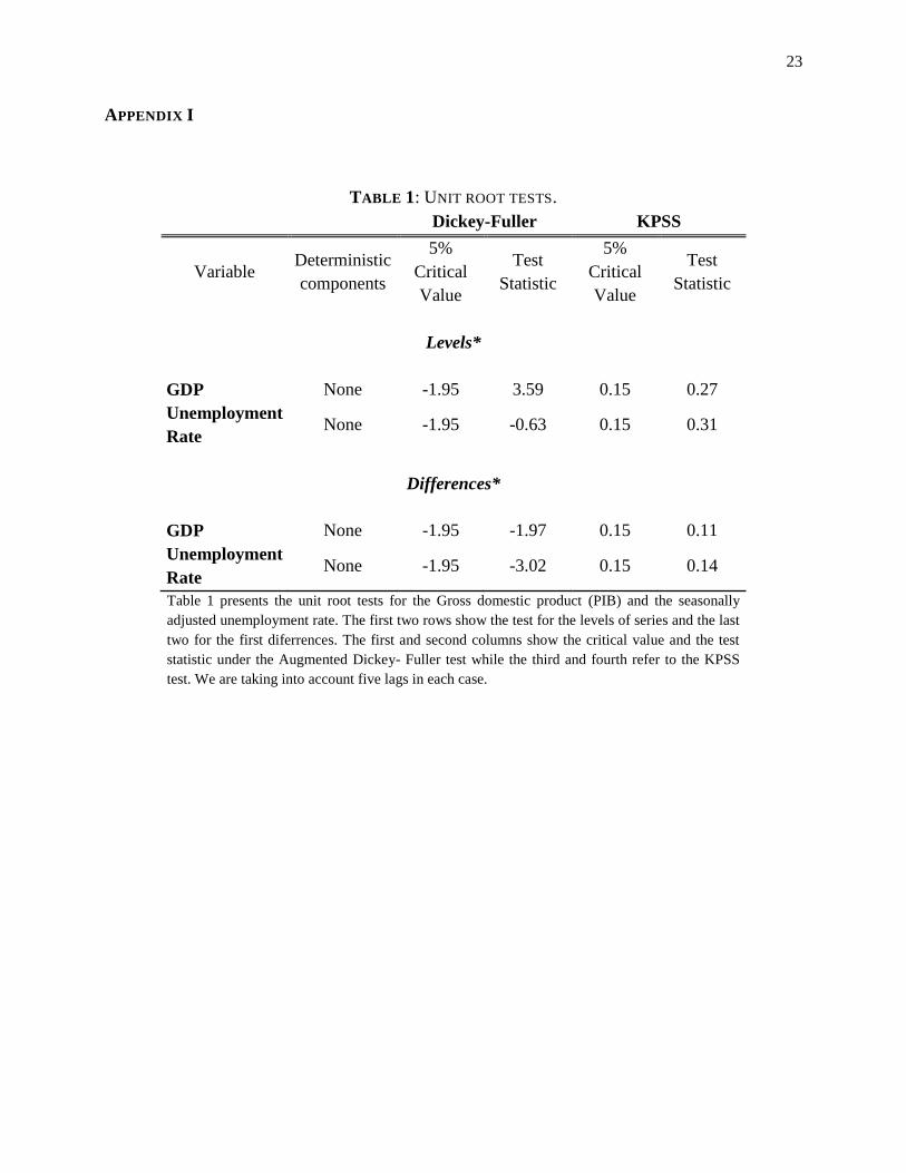
and the remaining series are integrated of order 1 as we present them in Appendix I.

3.2 STATIC RESPONSE

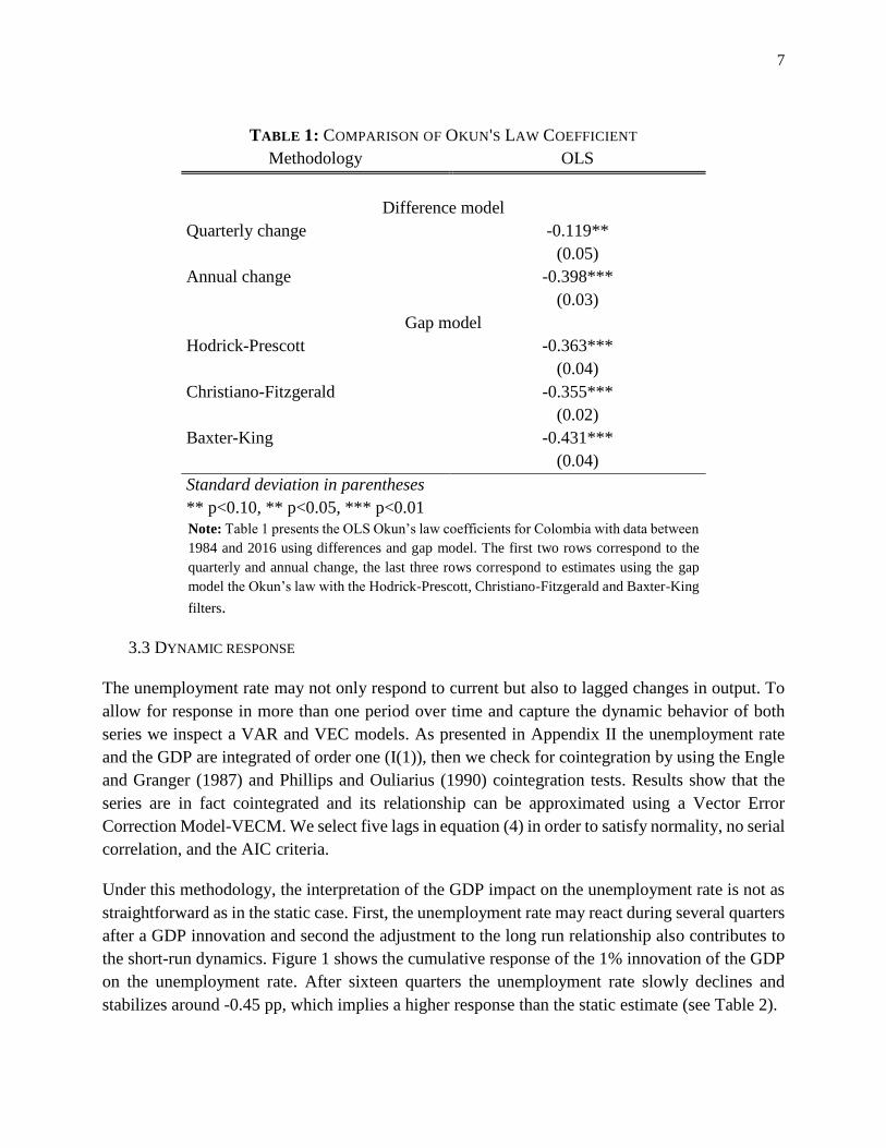
Table 1 presents the OLC estimates under five static specifications for the difference and gap

models (equations 1 and 2). The first panel corresponded to the quarterly and the annual change of

the variables, while the second panel corresponded to the estimates of the gap models using three

filters to decompose each time series among its cyclical and permanent component: Hodrick–

Prescott (1997), Christiano-Fitzgerald (2003) and Baxter-King (1999).

Thus, a 1% increment in the quarterly growth of the GDP reduces the unemployment rate by 0.12

pp, while a 1% increase in the annual growth reduces the unemployment rate by 0.40 pp. Hence,

the response with quarterly data is about one fourth of the one using annual changes; this fact is

consistent with findings by Knotek (2007). Also, estimates are similar to previous findings for

Colombia using quarterly data (see DANE (2006)). The OLC using annually change or filters

ranges from -0.35 pp to -0.44 pp similar to previous findings that use annual data in their

estimations (see González (2002), DANE (2006), Guillén (2010), Páez (2013), Cuervo y

Mondragón (2016)).

7

TABLE 1: COMPARISON OF OKUN'S LAW COEFFICIENT

Methodology OLS

Difference model

Quarterly change -0.119** (0.05)

Annual change -0.398*** (0.03)

Gap model

Hodrick-Prescott -0.363*** (0.04)

Christiano-Fitzgerald -0.355*** (0.02)

Baxter-King -0.431*** (0.04)

Standard deviation in parentheses

** p<0.10, ** p<0.05, *** p<0.01

Note: Table 1 presents the OLS Okun’s law coefficients for Colombia with data between

1984 and 2016 using differences and gap model. The first two rows correspond to the

quarterly and annual change, the last three rows correspond to estimates using the gap

model the Okun’s law with the Hodrick-Prescott, Christiano-Fitzgerald and Baxter-King

filters.

3.3 DYNAMIC RESPONSE

The unemployment rate may not only respond to current but also to lagged changes in output. To

allow for response in more than one period over time and capture the dynamic behavior of both

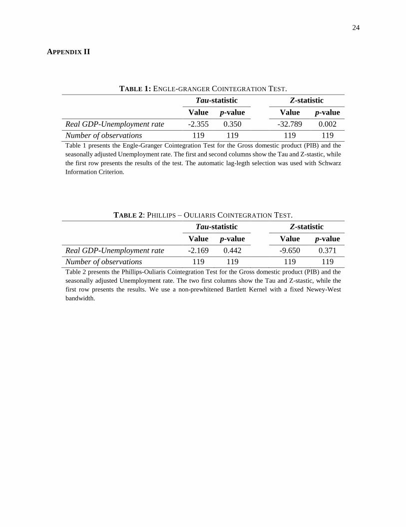
series we inspect a VAR and VEC models. As presented in Appendix II the unemployment rate

and the GDP are integrated of order one (I(1)), then we check for cointegration by using the Engle

and Granger (1987) and Phillips and Ouliarius (1990) cointegration tests. Results show that the

series are in fact cointegrated and its relationship can be approximated using a Vector Error

Correction Model-VECM. We select five lags in equation (4) in order to satisfy normality, no serial

correlation, and the AIC criteria.

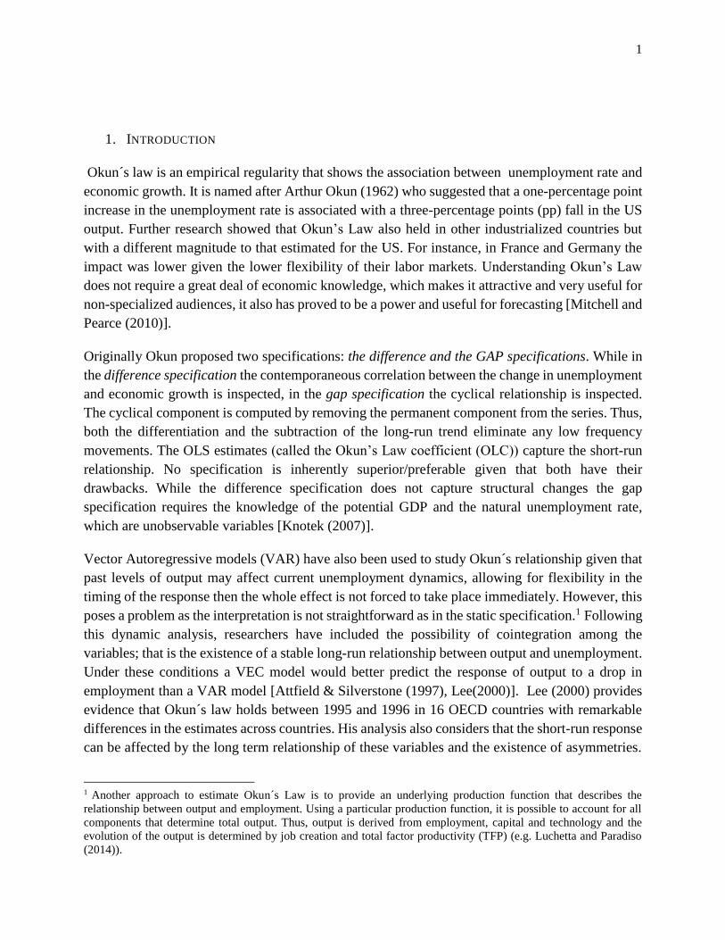
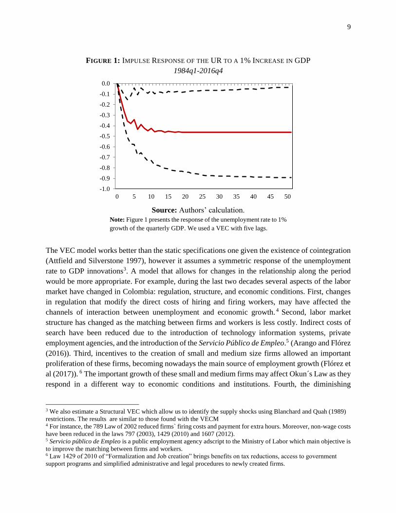
Under this methodology, the interpretation of the GDP impact on the unemployment rate is not as

straightforward as in the static case. First, the unemployment rate may react during several quarters

after a GDP innovation and second the adjustment to the long run relationship also contributes to

the short-run dynamics. Figure 1 shows the cumulative response of the 1% innovation of the GDP

on the unemployment rate. After sixteen quarters the unemployment rate slowly declines and

stabilizes around -0.45 pp, which implies a higher response than the static estimate (see Table 2).

8

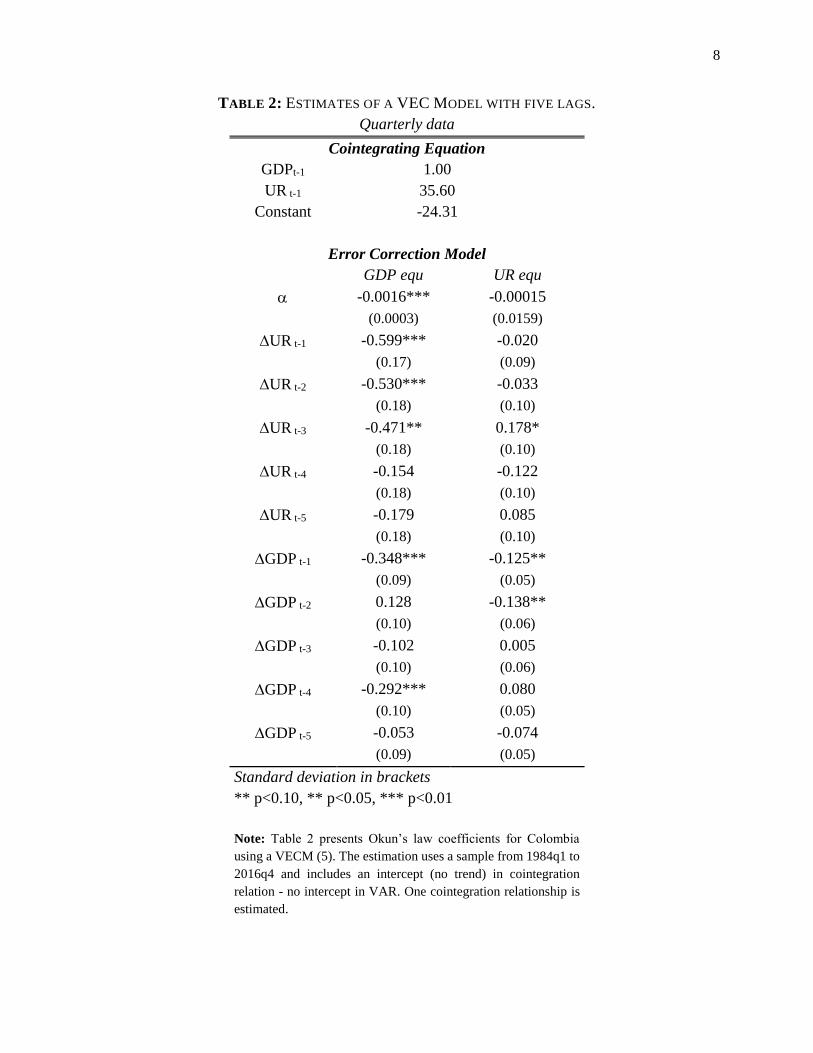
TABLE 2: ESTIMATES OF A VEC MODEL WITH FIVE LAGS.

Quarterly data

Cointegrating Equation

GDPt-1 1.00 UR t-1 35.60

Constant -24.31

Error Correction Model

GDP equ UR equ

-0.0016*** -0.00015

(0.0003) (0.0159)

UR t-1 -0.599*** -0.020

(0.17) (0.09)

UR t-2 -0.530*** -0.033

(0.18) (0.10)

UR t-3 -0.471** 0.178*

(0.18) (0.10)

UR t-4 -0.154 -0.122

(0.18) (0.10)

UR t-5 -0.179 0.085

(0.18) (0.10)

GDP t-1 -0.348*** -0.125**

(0.09) (0.05)

GDP t-2 0.128 -0.138**

(0.10) (0.06)

GDP t-3 -0.102 0.005

(0.10) (0.06)

GDP t-4 -0.292*** 0.080

(0.10) (0.05)

GDP t-5 -0.053 -0.074

(0.09) (0.05)

Standard deviation in brackets

** p<0.10, ** p<0.05, *** p<0.01

Note: Table 2 presents Okun’s law coefficients for Colombia

using a VECM (5). The estimation uses a sample from 1984q1 to

2016q4 and includes an intercept (no trend) in cointegration

relation - no intercept in VAR. One cointegration relationship is

estimated.

9

FIGURE 1: IMPULSE RESPONSE OF THE UR TO A 1% INCREASE IN GDP

1984q1-2016q4

Source: Authors’ calculation.

Note: Figure 1 presents the response of the unemployment rate to 1%

growth of the quarterly GDP. We used a VEC with five lags.

The VEC model works better than the static specifications one given the existence of cointegration

(Attfield and Silverstone 1997), however it assumes a symmetric response of the unemployment

rate to GDP innovations3. A model that allows for changes in the relationship along the period

would be more appropriate. For example, during the last two decades several aspects of the labor

market have changed in Colombia: regulation, structure, and economic conditions. First, changes

in regulation that modify the direct costs of hiring and firing workers, may have affected the

channels of interaction between unemployment and economic growth. 4 Second, labor market

structure has changed as the matching between firms and workers is less costly. Indirect costs of

search have been reduced due to the introduction of technology information systems, private

employment agencies, and the introduction of the Servicio Público de Empleo.5 (Arango and Flórez

(2016)). Third, incentives to the creation of small and medium size firms allowed an important

proliferation of these firms, becoming nowadays the main source of employment growth (Flórez et

al (2017)). 6 The important growth of these small and medium firms may affect Okun´s Law as they

respond in a different way to economic conditions and institutions. Fourth, the diminishing

3 We also estimate a Structural VEC which allow us to identify the supply shocks using Blanchard and Quah (1989)

restrictions. The results are similar to those found with the VECM 4 For instance, the 789 Law of 2002 reduced firms` firing costs and payment for extra hours. Moreover, non-wage costs

have been reduced in the laws 797 (2003), 1429 (2010) and 1607 (2012). 5 Servicio público de Empleo is a public employment agency adscript to the Ministry of Labor which main objective is

to improve the matching between firms and workers. 6 Law 1429 of 2010 of “Formalization and Job creation” brings benefits on tax reductions, access to government

support programs and simplified administrative and legal procedures to newly created firms.

-1.0

-0.9

-0.8

-0.7

-0.6

-0.5

-0.4

-0.3

-0.2

-0.1

0.0

0 5 10 15 20 25 30 35 40 45 50

10

importance of the minimum wage as determinant of both the natural unemployment rate and the

unemployment rate (see Arango, et al. (2016, 2017))7. Thus, it is rational to expect that changes on

the transmission channel of the minimum wage to the economy also change the relationship

between the unemployment rate and the GDP. Finally, after the economic crisis of the late nineties,

and the openness to international trade, there was an increase in the introduction of temporary

contracts that allows firms to respond in a more flexible way to an economic crisis and to be able

to compete internationally (Heckman and Pagés (2004)). All these changes in the labor market

across the last two decades might have changed the relation between UR and GDP across time.

Given these considerations we check for nonlinearities in each series and in the cointegration

context. First, we inspect evidence of unit root in a non-linear framework for the UR and GDP.

First, we used Andrews and Zivot (1992), Perron and Vogelsang (1992) and Clemente et al., (1988)

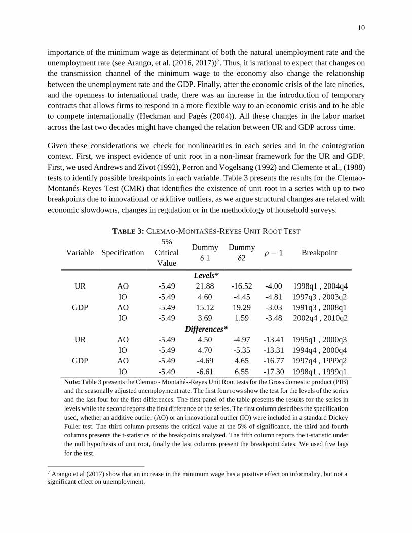
tests to identify possible breakpoints in each variable. Table 3 presents the results for the Clemao-

Montanés-Reyes Test (CMR) that identifies the existence of unit root in a series with up to two

breakpoints due to innovational or additive outliers, as we argue structural changes are related with

economic slowdowns, changes in regulation or in the methodology of household surveys.

TABLE 3: CLEMAO-MONTAÑÉS-REYES UNIT ROOT TEST

Variable Specification

5%

Critical

Value

Dummy

δ 1

Dummy

δ2 𝜌 − 1 Breakpoint

Levels*

UR AO -5.49 21.88 -16.52 -4.00 1998q1 , 2004q4

IO -5.49 4.60 -4.45 -4.81 1997q3 , 2003q2

GDP AO -5.49 15.12 19.29 -3.03 1991q3 , 2008q1

IO -5.49 3.69 1.59 -3.48 2002q4 , 2010q2

Differences*

UR AO -5.49 4.50 -4.97 -13.41 1995q1 , 2000q3

IO -5.49 4.70 -5.35 -13.31 1994q4 , 2000q4

GDP AO -5.49 -4.69 4.65 -16.77 1997q4 , 1999q2

IO -5.49 -6.61 6.55 -17.30 1998q1 , 1999q1

Note: Table 3 presents the Clemao - Montañés-Reyes Unit Root tests for the Gross domestic product (PIB)

and the seasonally adjusted unemployment rate. The first four rows show the test for the levels of the series

and the last four for the first differences. The first panel of the table presents the results for the series in

levels while the second reports the first difference of the series. The first column describes the specification

used, whether an additive outlier (AO) or an innovational outlier (IO) were included in a standard Dickey

Fuller test. The third column presents the critical value at the 5% of significance, the third and fourth

columns presents the t-statistics of the breakpoints analyzed. The fifth column reports the t-statistic under

the null hypothesis of unit root, finally the last columns present the breakpoint dates. We used five lags

for the test.

7 Arango et al (2017) show that an increase in the minimum wage has a positive effect on informality, but not a

significant effect on unemployment.

11

The first panel of the table presents the results for the levels of the series while the second reports

the results for the first differences. The first column describes the specification used, whether an

additive outlier (AO) or an innovational outlier (IO) were included in a standard Dickey Fuller test.

The second column presents the critical value at the 5% of significance, the third and fourth

columns present the t-statistics of the first and second breakpoints analyzed. The fifth column

reports the t-statistic for (𝜌 − 1) under the null hypothesis. Finally, the last column presents the

breakpoint dates. Results show the existence of structural changes and unit root in the series in

level. First, the t-statistic of IO and AO are significant at the 5% critical value, then we cannot

reject null hypothesis of unit root for the series in levels. Second, the first differences of both series

show evidence of stationarity with structural changes. These results are similar to those of the

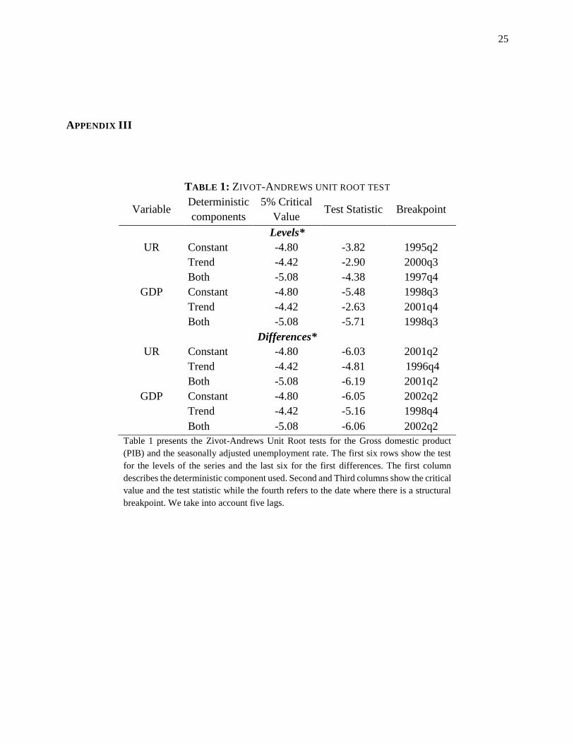
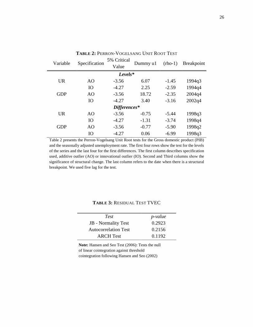
Andrews and Zivot and Perron and Vogelsang tests (see Appendix III). The breakpoints coincide

with the crises in the late nineties which had a strong effect over the Colombian economy, and the

methodological changes in the household surveys.

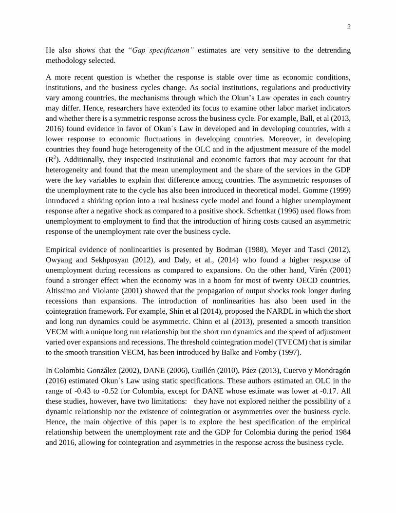
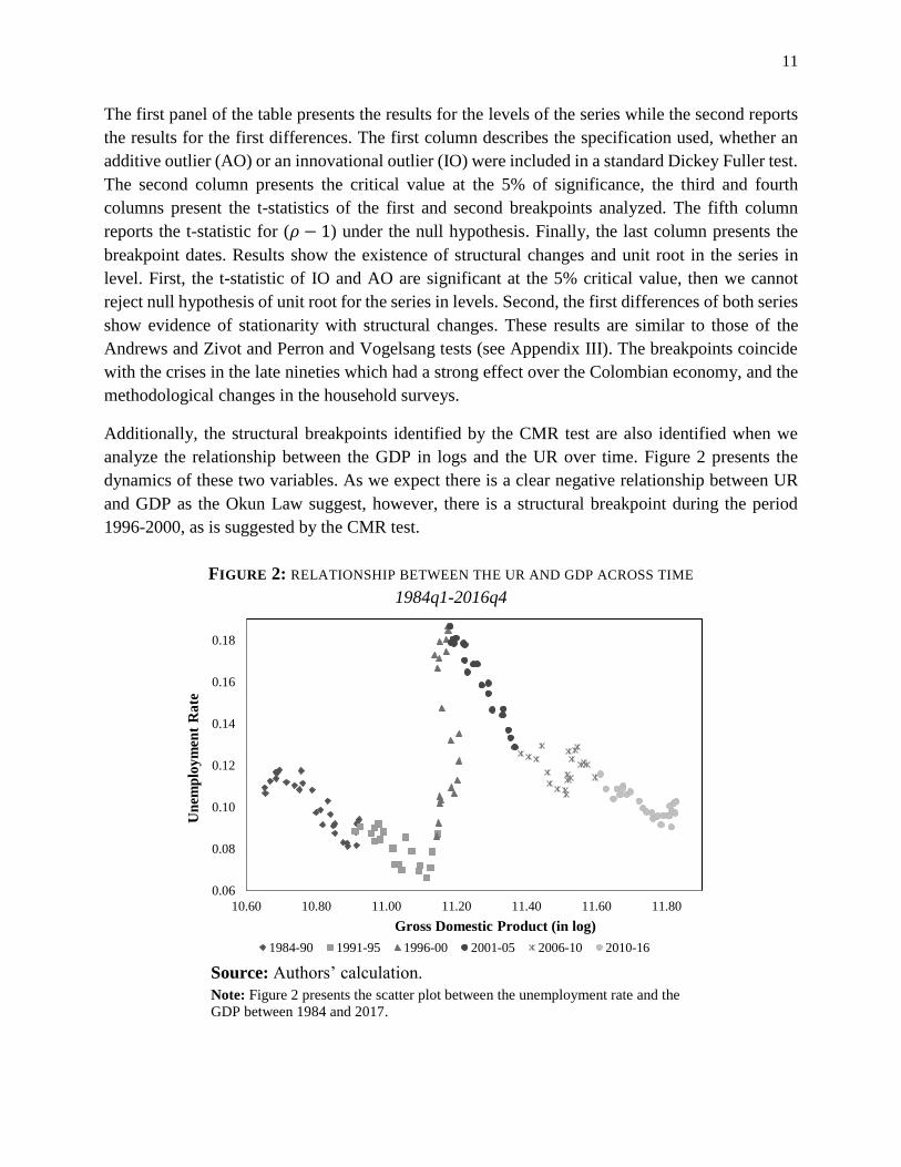
Additionally, the structural breakpoints identified by the CMR test are also identified when we

analyze the relationship between the GDP in logs and the UR over time. Figure 2 presents the

dynamics of these two variables. As we expect there is a clear negative relationship between UR

and GDP as the Okun Law suggest, however, there is a structural breakpoint during the period

1996-2000, as is suggested by the CMR test.

FIGURE 2: RELATIONSHIP BETWEEN THE UR AND GDP ACROSS TIME

1984q1-2016q4

Source: Authors’ calculation.

Note: Figure 2 presents the scatter plot between the unemployment rate and the

GDP between 1984 and 2017.

0.06

0.08

0.10

0.12

0.14

0.16

0.18

10.60 10.80 11.00 11.20 11.40 11.60 11.80

Un

emp

loy

men

t R

ate

Gross Domestic Product (in log)

1984-90 1991-95 1996-00 2001-05 2006-10 2010-16

12

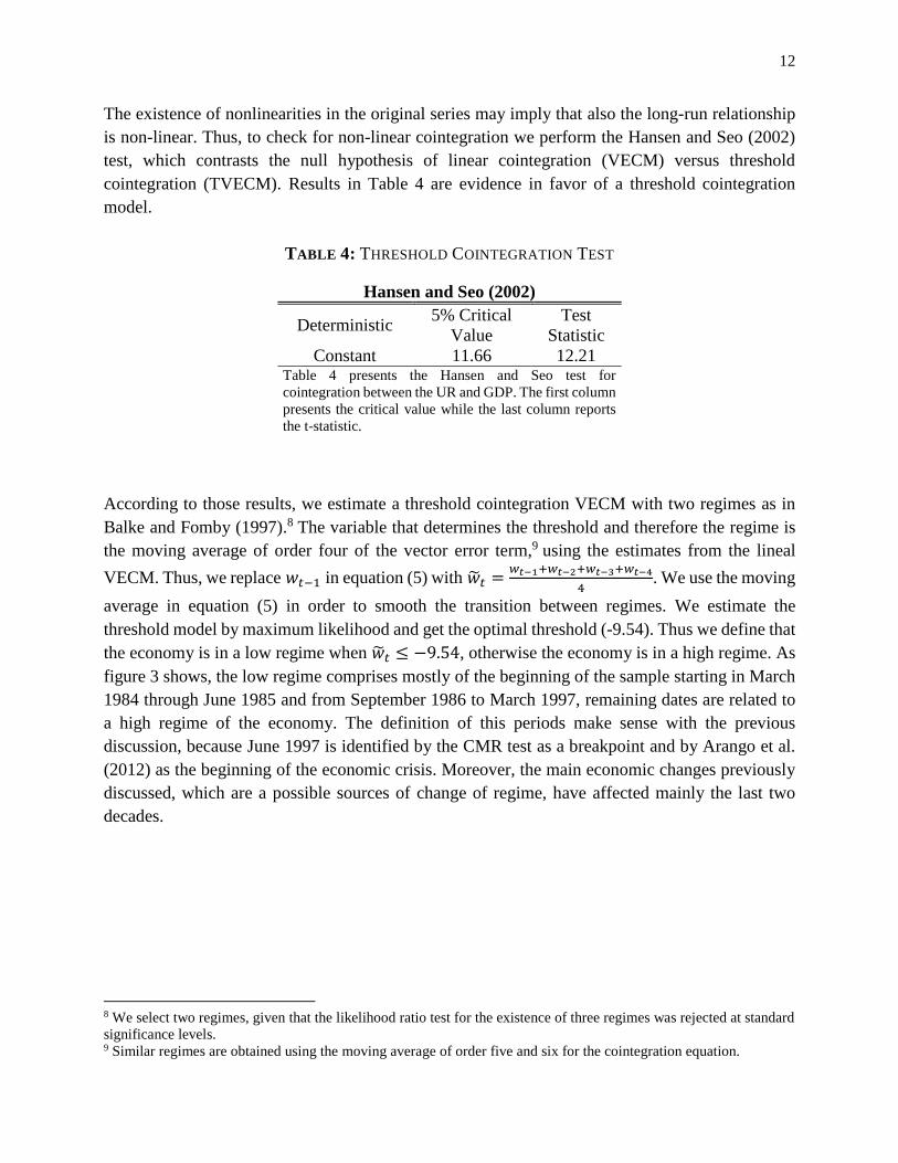
The existence of nonlinearities in the original series may imply that also the long-run relationship

is non-linear. Thus, to check for non-linear cointegration we perform the Hansen and Seo (2002)

test, which contrasts the null hypothesis of linear cointegration (VECM) versus threshold

cointegration (TVECM). Results in Table 4 are evidence in favor of a threshold cointegration

model.

TABLE 4: THRESHOLD COINTEGRATION TEST

Hansen and Seo (2002)

Deterministic 5% Critical

Value

Test

Statistic

Constant 11.66 12.21 Table 4 presents the Hansen and Seo test for

cointegration between the UR and GDP. The first column

presents the critical value while the last column reports

the t-statistic.

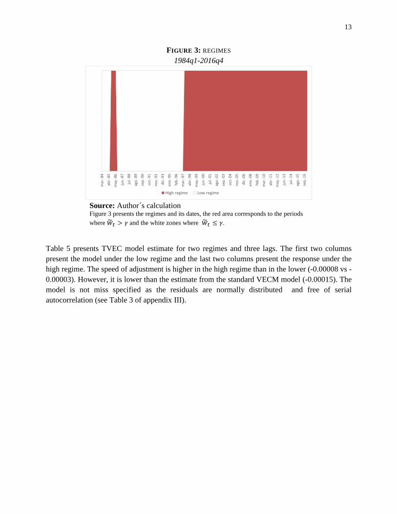
According to those results, we estimate a threshold cointegration VECM with two regimes as in

Balke and Fomby (1997).8 The variable that determines the threshold and therefore the regime is

the moving average of order four of the vector error term,9 using the estimates from the lineal

VECM. Thus, we replace 𝑤𝑡−1 in equation (5) with �̃�𝑡 =𝑤𝑡−1+𝑤𝑡−2+𝑤𝑡−3+𝑤𝑡−4

4. We use the moving

average in equation (5) in order to smooth the transition between regimes. We estimate the

threshold model by maximum likelihood and get the optimal threshold (-9.54). Thus we define that

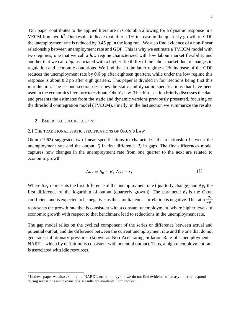
the economy is in a low regime when �̃�𝑡 ≤ −9.54, otherwise the economy is in a high regime. As

figure 3 shows, the low regime comprises mostly of the beginning of the sample starting in March

1984 through June 1985 and from September 1986 to March 1997, remaining dates are related to

a high regime of the economy. The definition of this periods make sense with the previous

discussion, because June 1997 is identified by the CMR test as a breakpoint and by Arango et al.

(2012) as the beginning of the economic crisis. Moreover, the main economic changes previously

discussed, which are a possible sources of change of regime, have affected mainly the last two

decades.

8 We select two regimes, given that the likelihood ratio test for the existence of three regimes was rejected at standard

significance levels. 9 Similar regimes are obtained using the moving average of order five and six for the cointegration equation.

13

FIGURE 3: REGIMES

1984q1-2016q4

Source: Author´s calculation Figure 3 presents the regimes and its dates, the red area corresponds to the periods

where �̃�𝑡 > 𝛾 and the white zones where �̃�𝑡 ≤ 𝛾.

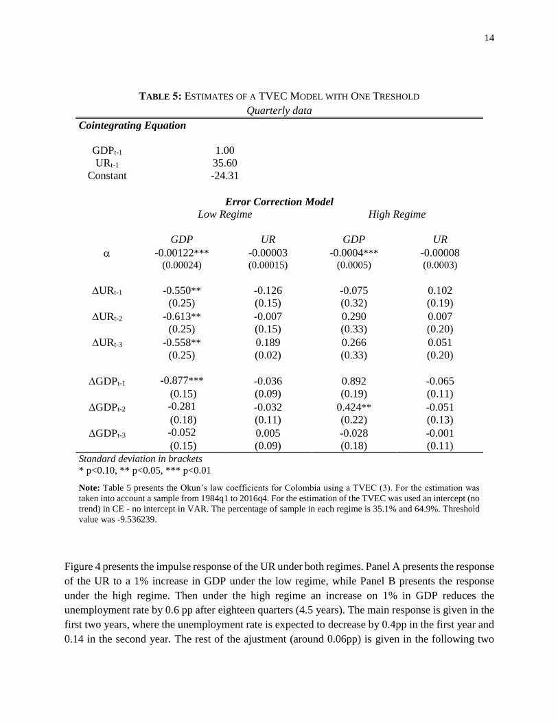
Table 5 presents TVEC model estimate for two regimes and three lags. The first two columns

present the model under the low regime and the last two columns present the response under the

high regime. The speed of adjustment is higher in the high regime than in the lower (-0.00008 vs -

0.00003). However, it is lower than the estimate from the standard VECM model (-0.00015). The

model is not miss specified as the residuals are normally distributed and free of serial

autocorrelation (see Table 3 of appendix III).

0%

10%

20%

30%

40%

50%

60%

70%

80%

90%

100%

mar

.-84

abr.

-85

may

.-86

jun

.-87

jul.-

88

ago

.-89

sep

.-90

oct

.-91

no

v.-9

2

dic

.-93

ene.

-95

feb

.-96

mar

.-97

abr.

-98

may

.-99

jun

.-00

jul.-

01

ago

.-02

sep

.-03

oct

.-04

no

v.-0

5

dic

.-06

ene.

-08

feb

.-09

mar

.-10

abr.

-11

may

.-12

jun

.-13

jul.-

14

ago

.-15

sep

.-16

High regime Low regime

14

TABLE 5: ESTIMATES OF A TVEC MODEL WITH ONE TRESHOLD

Quarterly data

Cointegrating Equation

GDPt-1 1.00

URt-1 35.60

Constant -24.31

Error Correction Model

Low Regime High Regime

GDP UR GDP UR

-0.00122*** -0.00003 -0.0004*** -0.00008(0.00024) (0.00015) (0.0005) (0.0003)

URt-1 -0.550** -0.126 -0.075 0.102

(0.25) (0.15) (0.32) (0.19)

URt-2 -0.613** -0.007 0.290 0.007

(0.25) (0.15) (0.33) (0.20)

URt-3 -0.558** 0.189 0.266 0.051

(0.25) (0.02) (0.33) (0.20)

GDPt-1 -0.877*** -0.036 0.892 -0.065

(0.15) (0.09) (0.19) (0.11)

GDPt-2 -0.281 -0.032 0.424** -0.051

(0.18) (0.11) (0.22) (0.13)

GDPt-3 -0.052 0.005 -0.028 -0.001

(0.15) (0.09) (0.18) (0.11)

Standard deviation in brackets

* p<0.10, ** p<0.05, *** p<0.01

Note: Table 5 presents the Okun’s law coefficients for Colombia using a TVEC (3). For the estimation was

taken into account a sample from 1984q1 to 2016q4. For the estimation of the TVEC was used an intercept (no

trend) in CE - no intercept in VAR. The percentage of sample in each regime is 35.1% and 64.9%. Threshold

value was -9.536239.

Figure 4 presents the impulse response of the UR under both regimes. Panel A presents the response

of the UR to a 1% increase in GDP under the low regime, while Panel B presents the response

under the high regime. Then under the high regime an increase on 1% in GDP reduces the

unemployment rate by 0.6 pp after eighteen quarters (4.5 years). The main response is given in the

first two years, where the unemployment rate is expected to decrease by 0.4pp in the first year and

0.14 in the second year. The rest of the ajustment (around 0.06pp) is given in the following two

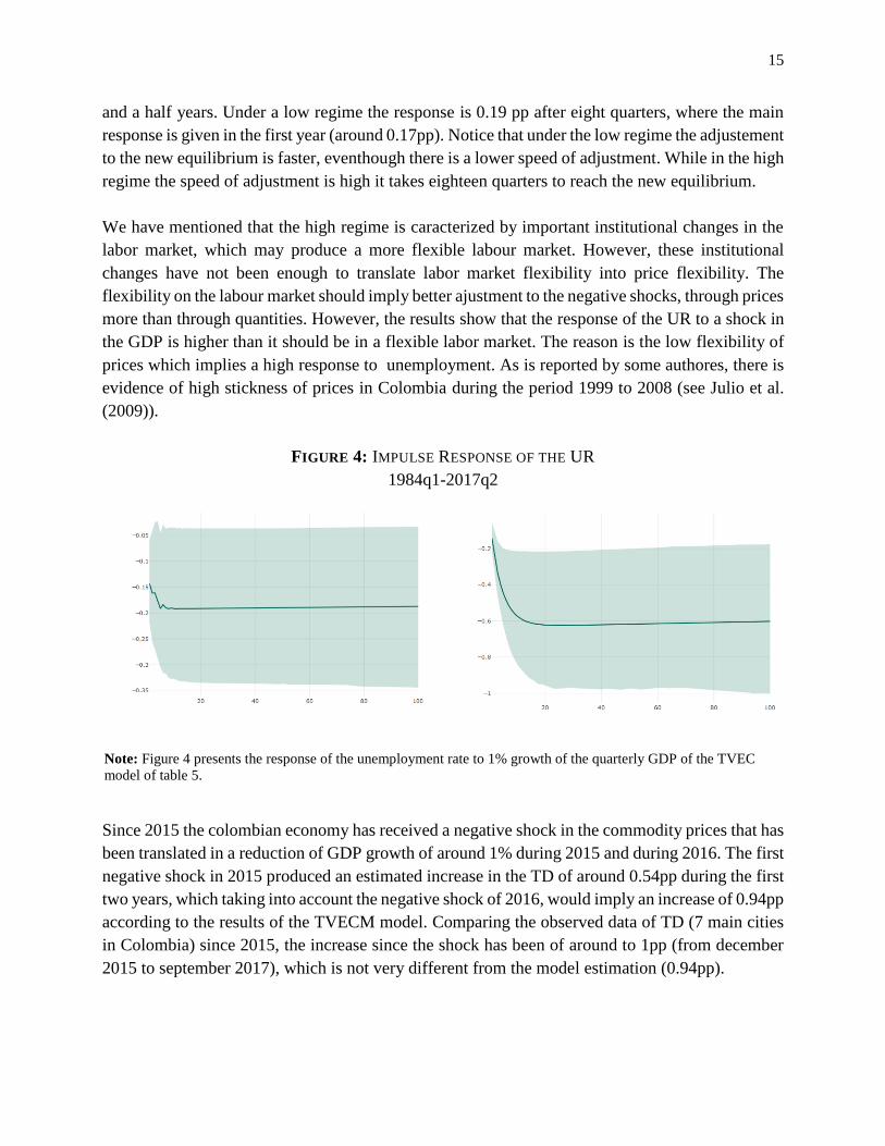
15

and a half years. Under a low regime the response is 0.19 pp after eight quarters, where the main

response is given in the first year (around 0.17pp). Notice that under the low regime the adjustement

to the new equilibrium is faster, eventhough there is a lower speed of adjustment. While in the high

regime the speed of adjustment is high it takes eighteen quarters to reach the new equilibrium.

We have mentioned that the high regime is caracterized by important institutional changes in the

labor market, which may produce a more flexible labour market. However, these institutional

changes have not been enough to translate labor market flexibility into price flexibility. The

flexibility on the labour market should imply better ajustment to the negative shocks, through prices

more than through quantities. However, the results show that the response of the UR to a shock in

the GDP is higher than it should be in a flexible labor market. The reason is the low flexibility of

prices which implies a high response to unemployment. As is reported by some authores, there is

evidence of high stickness of prices in Colombia during the period 1999 to 2008 (see Julio et al.

(2009)).

FIGURE 4: IMPULSE RESPONSE OF THE UR

1984q1-2017q2

Note: Figure 4 presents the response of the unemployment rate to 1% growth of the quarterly GDP of the TVEC

model of table 5.

Since 2015 the colombian economy has received a negative shock in the commodity prices that has

been translated in a reduction of GDP growth of around 1% during 2015 and during 2016. The first

negative shock in 2015 produced an estimated increase in the TD of around 0.54pp during the first

two years, which taking into account the negative shock of 2016, would imply an increase of 0.94pp

according to the results of the TVECM model. Comparing the observed data of TD (7 main cities

in Colombia) since 2015, the increase since the shock has been of around to 1pp (from december

2015 to september 2017), which is not very different from the model estimation (0.94pp).

16

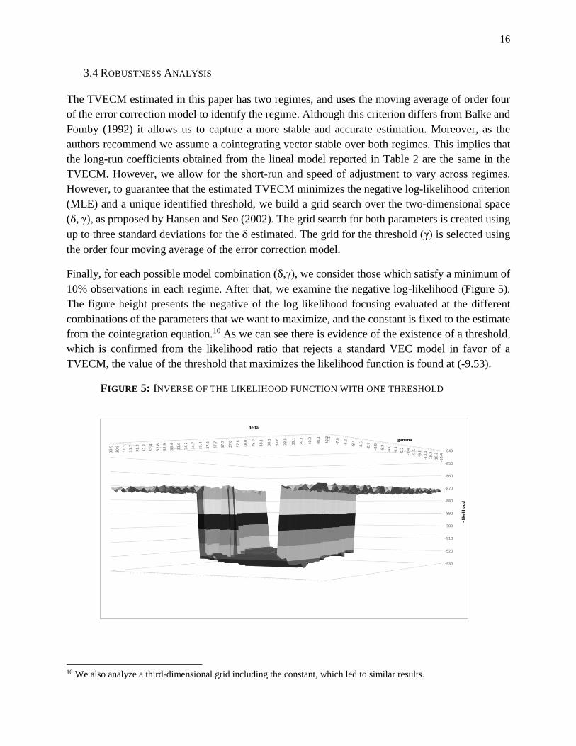
3.4 ROBUSTNESS ANALYSIS

The TVECM estimated in this paper has two regimes, and uses the moving average of order four

of the error correction model to identify the regime. Although this criterion differs from Balke and

Fomby (1992) it allows us to capture a more stable and accurate estimation. Moreover, as the

authors recommend we assume a cointegrating vector stable over both regimes. This implies that

the long-run coefficients obtained from the lineal model reported in Table 2 are the same in the

TVECM. However, we allow for the short-run and speed of adjustment to vary across regimes.

However, to guarantee that the estimated TVECM minimizes the negative log-likelihood criterion

(MLE) and a unique identified threshold, we build a grid search over the two-dimensional space

(δ, γ), as proposed by Hansen and Seo (2002). The grid search for both parameters is created using

up to three standard deviations for the δ estimated. The grid for the threshold (γ) is selected using

the order four moving average of the error correction model.

Finally, for each possible model combination (δ,γ), we consider those which satisfy a minimum of

10% observations in each regime. After that, we examine the negative log-likelihood (Figure 5).

The figure height presents the negative of the log likelihood focusing evaluated at the different

combinations of the parameters that we want to maximize, and the constant is fixed to the estimate

from the cointegration equation.10 As we can see there is evidence of the existence of a threshold,

which is confirmed from the likelihood ratio that rejects a standard VEC model in favor of a

TVECM, the value of the threshold that maximizes the likelihood function is found at (-9.53).

FIGURE 5: INVERSE OF THE LIKELIHOOD FUNCTION WITH ONE THRESHOLD

10 We also analyze a third-dimensional grid including the constant, which led to similar results.

30

.9

30

.9

31

.3

31

.7

31

.9

32

.3

32

.4

32

.8

32

.9

33

.4

33

.6

34

.2

34

.7

35

.4

37

.3

37

.7

37

.7

37

.8

37

.8

38

.0

38

.0

38

.1

38

.1

38

.6

38

.9

39

.1

39

.7

40

.0

40

.1

40

.3

-930

-920

-910

-900

-890

-880

-870

-860

-850

-840

-10

.4-1

0.2

-10

.2

-10

.0

-9.8

-9.6

-9.4

-9.2

-9.1

-9.0

-8.9

-8.8

-8.7

-8.5

-8.4

-8.2

-7.6

-7.1

-likelih

ood

gamma

delta

17

4. FINAL REMARKS.

This paper estimates a non-linear cointegration model (TVEC) that seems to be the best empirical

specification to capture the Okun´s Law in Colombia from 1984-2017. Following the traditional

literature we estimate the first-differences model, which suggests that an increase of 1% in the

quarterly growth of the GDP reduces unemployment rate by 0.12 pp, while a 1% increase in the

annual growth reduces unemployment rate by 0.40 pp. We also estimate the GAP specification

where the OL coefficients range from -0.35 pp to -0.44 pp. These results are similar to previous

findings estimated for Colombia (see González (2002), DANE (2006), Guillén (2010), Páez (2013),

Cuervo y Mondragón (2016)).

A lineal and non-linear cointegration approach has not been used before in Colombian case to

estimate the OL. Results from a lineal VECM estimation, show that after 1% increase in the GDP,

the unemployment rate is reduced by 0.45 pp after sixteen quarters. However, according to our

results, a non-linear cointegration approach (TVECM) seems to be a better empirical

approximation. We estimate two-regimes in relation to the moving average of order four of the

error-correction term. We find evidence of a higher response in the current regime (high regime),

than in the lower regime. Under a high regime, an increase of 1% in GDP reduces the UR by 0.6pp

after eighteen quarters (4.5 years), while in the low regime the response is 0.19 pp after eight

quarters (2 years).

We define the high regime as a regime that has been characterized by important transformations in

the Colombian labor market. During the last two decades, several aspects of the labor market have

changed: i) changes in the regulation that modify the direct cost of hiring and firing workers, ii)

increase in matchng efficiency between firms and workers, due to the introduction of technology

information systems, and private and public employment agencies, such as the Servicio Publico de

Empleo, iii) major incentives for the creation of small and medium size firms, which nowadays are

one of the main sources of employment growth and (Flórez et al (2017)), iv) change of the role of

minimum wage as being less important determinant of the natural unemployment rate or the

unemployment rate in Colombia (see Arango, et al. (2016, 2017))11, v) finally, after the economic

crisis of the late nineties, and the openness to international trade, there was an increase on the

introduction of temporary contracts that allowed firms to respond in a more flexible way to

economic crisis and to be able to compete internationally (Heckman and Pagés (2004)).

All these changes in the labor market across the last two decades might have changed the relation

between UR and GDP across time, making the labor market more flexible. Some evidence of this

flexibility in the labor market is reflected the increase of worker mobility across estates

(employment, unemployment and non-participant) found by Lasso (2013) as well as the growth in

11 Arango et al. (2017) show that an increase on the minimum wage have a positive effect on the informality but not a

significant effect on the unemployment.

18

churning and workers reallocation rates in Colombia for the period 2009-2015 found by Flórez, et

al. (2017) and Morales and Medina (2016).

We have mentioned that the high regime is caracterized by important institutional changes in the

labor market, which may imply a more flexible labour market. However, these institutional changes

have not been sufficient to translate labor market flexibility into price flexibility. The flexibility of

the labour market should imply a better ajustment to negative shocks through prices more than

quantities. However, the results of the TVECM model show that under a high regime the response

of the UR to a shock in the GDP is higher than it should be in a flexible labor market, where the

ajustment should be given by reduction/increase on wages instead of increase/reduction of

unemployment. The reason is the low flexibility of prices (Julio et al. 2009), which implies a high

response through unemployment.

Since 2015 the colombian economy has received a negative shock in the commodity prices that has

been translated into a reducción of GDP growth of around 1% during 2015 and during 2016.

According to the TVECM model these two negative shocks would imply an estimated increase in

the TD of around 0.94pp after the two previous years. However, since 2015, the increase in the TD

(seven main cities) has been of around 1pp (from december 2015 to september 2017). Even though,

the final effect would be observed in the next two years.

The estimation of a non-linear cointegration model of the Okun Law in the case of Colombia

produces very usefull and interesting results that call for further research. The results of the paper

are usefull for policy makers to forecast the response of the unemployment rate under a negative

shock to the GDP, as has been the case with the current (2015-2017) slowdown of economic

growth. Given the atipic historical behavior of the colombian unemployment rate, more non-linear

methodologies can be implemented in order to improve our knowledge of labour market dynamics,

and explore the change in the relation between the unemployment rate and the GDP growth.

19

REFERENCES

Alfonso, V., Arango, L., Arias, F., Cangrejo, G., & Pulido, J. (2012). Ciclos de Negocios en

Colombia: 1975-2011, Borradores de Economía, (651). Banco de la República de Colombia.

Altissimo, F., & Violante, G. L. (2001). The nonlinear dynamics of output and unemployment in

the U.S, Journal of Applied Economics., vol.16, 461–486.

Arango, L.E., García, A. F., & Posada, C. E. (2008). La metodología de la Encuesta Continua de

Hogares y el empalme de las series del mercado laboral urbano de Colombia. Desarrollo y

Sociedad, (61), 207-248.

Arango, L. E., & Flórez, L. A. (2016). Determinants of Structural Unemployment in Colombia: a

Search Approach. Borradores de Economía, (969).

Arango, L. E., & Flórez, L. A. (2017). Informalidad laboral y elementos para un salario mínimo

diferencial por regiones en Colombia (No. 1023). Banco de la Republica de Colombia.

Attfield, L.F., & Brian, S. (1997). Okun’s Coefficient: A Comment. Review of Economics and

Statistics, vol.79, 326 – 329.

Balke, N., & Fomby, T., (1997). Threshold Cointegration. International Economic Review, vol.

38(3), 627-45.

Ball, L. M., Leigh, D., & Loungani, P. (2013). Okun's Law: Fit at Fifty?, NBER Working Papers

18668, National Bureau of Economic Research.

Ball, L. M., Furceri, D., Leigh, D., & Loungani, P. (2016). Does One Law Fit All ? Cross- Country

Evidence on Okun ’s Law. Paper Presented at the IMF-OCP Workshop on Global Labour Markets.

Blanchard, O. J.; Quah, D. (1989). The Dynamic Effects of Aggregate Demand and Supply

Disturbances, American Economic Review, vol. 79, 4, pp. 655-673.

Baxter, M. & King, R. (1999). Measuring Business Cycles: Approximate Band-Pass Filters For

Economic Time Series. The Review of Economics and Statistics, vol. 81(4), 575-593.

Binet, M., & Francois, F. (2013). Okun's law in the french regions: a cross-regional comparison.

Economics Bulletin, AccessEcon, vol. 33(1), 420-433.

Bodman, P. M. (1998). Asymmetry and Duration Dependence in Australian GDP and

Unemployment. Economic Record, Vol.74(227), 399 – 411.

Chinn, M. D., Ferrara, L., & Mignon, V. (2013). Post-Recession Us Employment Through the Lens

of a Nonlinear Okun's Law. NBER Working Paper No. w19047.

Christiano, J. & Fitzgerald, J., (2003). The Band Pass Filter. International Economic Review,

Department of Economics, University of Pennsylvania and Osaka University Institute of Social

and Economic Research Association, vol. 44(2), 435-465, 05.

Clemente, J., Montañés, A., & Reyes, M., (1998). Testing for a unit root in variables with a double

change in the mean. Economics Letters, vol. 59(2), 175-182.

20

Crespo, J. (2003). Okun's Law Revisited. Oxford Bulletin of Economics and Statistics, Department

of Economics, University of Oxford, vol. 65(4), 439-451.

Cuervo, D., & Mondragón, J. (2016). Respuesta del producto a perturbaciones de oferta y demanda

en Colombia: 1981-2015. Econografos Centro de investigaciones para el Desarrollo (CID).

Daly, M., Fernald, J., Jorda, O., & Nechio, F. (2012). Okun’s Macroscope: Output and Employment

after the great recession. Federal Reserve Bank of San Francisco.

DANE. (2006). Ejercicios econométricos para evaluar los cambios en las principales variables

laborales y su relación con el desempeño económico. Revista/Journal: Anexos comisión GEIH.

Engle, R., & Granger, C., (1987). Co-integration and Error Correction: Representation, Estimation,

and Testing. Econometrica, Vol. 55(2), 251-76.

Gomme, P., (1999). Shirking, Unemployment and Aggregate Fluctuations. International Economic

Review, Department of Economics, University of Pennsylvania and Osaka University Institute of

Social and Economic Research Association, vol. 40(1), 3-21.

González, J. A., (2002). Labor market flexibility in thirteen Latin American countries and the

United States: Revisiting and Expanding Okun coefficients, Center for Research on Economic

Development and Policy Reform - Working paper No. 136 Stanford University.

Guillén, A. L. (2010). La Ley de Okun para la economía colombiana, periodo 1985-2009,

Observatorio de la Economía Latinoamericana, N°135.

Heckman, J. and Pagés, C. (2003). Law and employment: Lessons from Latin America and the

Caribbean (No. w10129). National Bureau of Economic Research.

Hamilton, J. D. (1994). Time series analysis, Princeton University Press, Princeton, NJ.

Hansen, B., & Seo, B. (2002). Testing for two-regime threshold cointegration in vector error-

correction models. Journal of Econometrics, vol. 110(2), 293-318.

Hodrick, R. & Prescott, E,. (1997). Postwar U.S. Business Cycles: An Empirical Investigation.

Journal of Money, Credit, and Banking, vol. 29 (1), 1–16

Huang, H.-C., Yeh, C.-C., Ku, K.-P., & Lin, S.-C. (2016). The effects of inflation targeting on

Okun’s law. Applied Economics Letters, vol. 23(12), 868–874.

Johansen, S., (1988). Statistical Analysis of Cointegration Vectors, Journal of Economic Dynamics

and Control, Vol. 12(2–3), 231–254.

Johansen, S., (1991). Estimation and Hypothesis Testing of Cointegration Vectors in Gaussian

Vector Autoregressive Models. Econometrica, Vol. 59(6), 1551–1580.

Julio, J. M., Zárate, H. M., & Hernández, M. D. (2010). The Stickiness of Colombian Consumer

Prices. Ensayos sobre Política Económica, 28(63), 100-152.

Kapetanios, G., Shin, Y., & Snell, A. (2006). Testing for cointegration in nonlinear smooth

transition error correction models. Econometric Theory, 22, 279-303.

21

Knotek II, E. S., (2007). How useful is Okun's law?. Economic Review, Federal Reserve Bank of

Kansas City, issue Q IV, 73-103.

Lasso, F. J. (2013). La dinámica del desempleo urbano en Colombia. En L. E. Arango, & F.

Hamann, El mercado de trabajo en Colombia: hechos, tendencias e instituciones. Banco de la

República. Cap. 3, 131 - 166.

Lee, Jim., (2000). The Robustness of Okun´s Law: Evidence from OECD Countries, Journal of

Macroeconomics, vol. 22 (2), 331-356.

Lucchetta, M., & Paradiso, A. (2014). Sluggish US employment recovery after the Great

Recession: Cyclical or structural factors?, Economics Letters, Elsevier, vol. 123(2),109-112.

Morales, L. F., & Medina, D. (2016). Labor Fluidity and Performance of Labor Outcomes in

Colombia: Evidence from Employer-Employee Linked Panel. Borradores de Economía, (926)

Meyer, B., & Tasci, M. (2012). An unstable Okun’s Law, not the best rule of thumb. Economic

Commentary, 2012-08.

Mitchell, K., & Pearce, D.K., 2010, Do Wall Street Economists Believe in Okun’s Law and the

Taylor Rule?. Journal of Economics and Finance, Vol. 34, 196 -217.

Okun, A.M. (1962). Potential GNP: its measurement and significance, in American statistical

association. Proceedings of the Business and Economics Statistics, 98–104.

Owyang, M., & Sekhposyan, T. (2012). Okun’s law over the business cycle: Was the great

recession all that different? Federal Reserve Bank of St. Louis Review. Vol. 94(4), 399-418.

Páez, N., (2013), Una revisión de la Ley de Okun para Latinoamérica. Tesis de maestría, Editorial:

Universidad del Valle Cali, Colombia.

Perman, R., Stephan, G., & Tavéra, C. (2015). Okun’s Law a Meta-analysis. Manchester School,

83(1), 101–126.

Perron, P., & Vogelsang, T. (1992), Testing for a Unit Root in a Time Series with a Changing

Mean: Corrections and Extensions, Journal of Business & Economic Statistics, vol.10 (4), 467-70.

Phillips, P., & Ouliaris, S. (1990). “Asymptotic Properties of Residual Based Tests for

Cointegration” Econometrica, Vol. 58(1), 165-93.

Psaradakis, Z., Sola, M., & Spagnolo, F. (2004). On Markov error-correction models, with an

application to stock prices and dividends. Journal of Applied Econometrics, vol. 19, 69-88.

Schettkat, R. (1996). Labor Market Flows Over the Business Cycle: An Asymmetric Hiring Cost

Explanation. Journal of Institutional and Theoretical Economics (JITE) / Zeitschrift Für Die

Gesamte Staatswissenschaft, vol. 152(4), 641-653.

Seo, M. H., (2006). Bootstrap testing for the null of no cointegration in a threshold vector error

correction model. Journal of Econometrics, vol. 134(1), 129-150.

22

Shin, Y., Yu, B., & Greenwood-Nimmo, M. (2014). Modelling Asymmetric Cointegration and

Dynamic Multipliers in a Nonlinear ARDL Framework, in "Festschrift in Honor of Peter Schmidt:

Econometric Methods and Applications", editor "Sickles, Robin C. and Horrace, William C."

Viren, Matti. (2001). The Okun Curve is Nonlinear. Economics Letters, vol. 70(2), 253-257

Zidong, A., Nathalie, G. P., Prakash, L., & Saurabh, M. (2016). Does Growth Create Jobs?

Evidence for Advanced and Developing Economies. IMF RESEARCH, vol.17(3), 27.

Zivot, E., & Andrews, D. (1992). Further Evidence on the Great Crash, the Oil-Price Shock, and

the Unit-Root Hypothesis. Journal of Business & Economic Statistics, vol.10(3), 251-270.

23

APPENDIX I

TABLE 1: UNIT ROOT TESTS.

Dickey-Fuller KPSS

Variable Deterministic

components

5%

Critical

Value

Test

Statistic

5%

Critical

Value

Test

Statistic

Levels*

GDP None -1.95 3.59 0.15 0.27

Unemployment

Rate None -1.95 -0.63 0.15 0.31

Differences*

GDP None -1.95 -1.97 0.15 0.11

Unemployment

Rate None -1.95 -3.02 0.15 0.14

Table 1 presents the unit root tests for the Gross domestic product (PIB) and the seasonally

adjusted unemployment rate. The first two rows show the test for the levels of series and the last

two for the first diferrences. The first and second columns show the critical value and the test

statistic under the Augmented Dickey- Fuller test while the third and fourth refer to the KPSS

test. We are taking into account five lags in each case.

24

APPENDIX II

TABLE 1: ENGLE-GRANGER COINTEGRATION TEST.

Tau-statistic Z-statistic

Value p-value Value p-value

Real GDP-Unemployment rate -2.355 0.350 -32.789 0.002

Number of observations 119 119 119 119

Table 1 presents the Engle-Granger Cointegration Test for the Gross domestic product (PIB) and the

seasonally adjusted Unemployment rate. The first and second columns show the Tau and Z-stastic, while

the first row presents the results of the test. The automatic lag-legth selection was used with Schwarz

Information Criterion.

TABLE 2: PHILLIPS – OULIARIS COINTEGRATION TEST.

Tau-statistic Z-statistic

Value p-value Value p-value

Real GDP-Unemployment rate -2.169 0.442 -9.650 0.371

Number of observations 119 119 119 119

Table 2 presents the Phillips-Ouliaris Cointegration Test for the Gross domestic product (PIB) and the

seasonally adjusted Unemployment rate. The two first columns show the Tau and Z-stastic, while the

first row presents the results. We use a non-prewhitened Bartlett Kernel with a fixed Newey-West

bandwidth.

25

APPENDIX III

TABLE 1: ZIVOT-ANDREWS UNIT ROOT TEST

Variable Deterministic

components

5% Critical

Value Test Statistic Breakpoint

Levels*

UR Constant -4.80 -3.82 1995q2

Trend -4.42 -2.90 2000q3

Both -5.08 -4.38 1997q4

GDP Constant -4.80 -5.48 1998q3

Trend -4.42 -2.63 2001q4

Both -5.08 -5.71 1998q3

Differences*

UR Constant -4.80 -6.03 2001q2

Trend -4.42 -4.81 1996q4

Both -5.08 -6.19 2001q2

GDP Constant -4.80 -6.05 2002q2

Trend -4.42 -5.16 1998q4

Both -5.08 -6.06 2002q2

Table 1 presents the Zivot-Andrews Unit Root tests for the Gross domestic product

(PIB) and the seasonally adjusted unemployment rate. The first six rows show the test

for the levels of the series and the last six for the first differences. The first column

describes the deterministic component used. Second and Third columns show the critical

value and the test statistic while the fourth refers to the date where there is a structural

breakpoint. We take into account five lags.

26

TABLE 2: PERRON-VOGELSANG UNIT ROOT TEST

Variable Specification 5% Critical

Value Dummy u1 (rho-1) Breakpoint

Levels*

UR AO -3.56 6.07 -1.45 1994q3

IO -4.27 2.25 -2.59 1994q4

GDP AO -3.56 18.72 -2.35 2004q4

IO -4.27 3.40 -3.16 2002q4

Differences*

UR AO -3.56 -0.75 -5.44 1998q3

IO -4.27 -1.31 -3.74 1998q4

GDP AO -3.56 -0.77 -5.90 1998q2

IO -4.27 0.06 -6.99 1998q3

Table 2 presents the Perron-Vogelsang Unit Root tests for the Gross domestic product (PIB)

and the seasonally adjusted unemployment rate. The first four rows show the test for the levels

of the series and the last four for the first differences. The first column describes specification

used, additive outlier (AO) or innovational outlier (IO). Second and Third columns show the

significance of structural change. The last column refers to the date when there is a structural

breakpoint. We used five lag for the test.

TABLE 3: RESIDUAL TEST TVEC

Test p-value

JB - Normality Test 0.2923

Autocorrelation Test 0.2156

ARCH Test 0.1192

Note: Hansen and Seo Test (2006): Tests the null

of linear cointegration against threshold

cointegration following Hansen and Seo (2002)

ogotá -