no. 574 identifying the bank lending channel in brazil

No. 574

Identifying the bank lending channel in

Brazil through data frequency

Christiano A. Coelho João M. P. de Mello Márcio G. P. Garcia

TEXTO PARA DISCUSSÃO

DEPARTAMENTO DE ECONOMIA www.econ.puc-rio.br

1

Identifying the bank lending channel in Brazil

through data frequency §

Christiano A Coelho†, João M P De Mello‡ and Márcio G. P. Garcia¥

Abstract

Using the different response timings of credit demand and supply, we

isolate supply shifts after monetary policy shocks. We show that the

bank lending channel exists in Brazil: after an increase (decrease) in

the basic interest rate (Selic), banks reduce (increase) the quantity of

new loans and raise (lower) interest rates. However, contrary to the

empirical literature for the US, we find evidence that large banks react

more than smaller ones to monetary policy shocks. Results may have

important implications for monetary policy transmission in light of the

recent wave of concentration in the Brazilian banking industry.

KEY WORDS: monetary policy transmission; credit markets; bank

lending channel.

JEL CODES: E52; E58.

This version: May 3rd, 2010

§We would like to thank Arturo Galindo, Roberto Rigobon, Sérgio Werlang, Márcio Nakane, Leonardo Rezende, Juliano Assunção and our editor Claudio Raddatz for insightful comments. Opinions expressed here are solely from the authors, and do not reflect any official position of the Central Bank of Brazil. † Central Bank of Brazil and Departamento de Economia, PUC-Rio: [email protected]. . ‡ Departamento de Economia, PUC-Rio: [email protected]. ¥ Departamento de Economia, PUC-Rio: [email protected].

2

I. Introduction

Monetary policy affects economic activity through different channels. One

mechanism is the credit channel, i.e., how monetary policy impacts the real sector

through its effect on the functioning of credit markets (Bernanke and Blinder [1988],

Bernanke and Gertler [1989], Bernanke, Gertler and Gilchrist [2000] and Kyiotaki and

Moore [1997]). There are two types of credit channels: the broad credit channel and the

bank lending channel. The former is the channel through which monetary policy affects

the balance sheet of lenders and borrowers in the economy.

Banks fund a significant part of their operation issuing deposits, normally the

cheapest way to get funding. Assuming that deposits and other source of funding are

less-than-perfect substitutes, monetary policy, insofar as it affects the amount of deposits

in the banking system, will shift the supply schedule of bank credit, a transmission

mechanism known as the bank lending channel.

Bernanke and Blinder [1992] first tried to identify the bank lending channel by

looking at the relationship between monetary policy shocks and future amounts of loans.

Interpretation of their empirical results is blurred by the fact that, several months ahead of

a monetary policy shock, aggregate lending changes because of both supply (bank

lending channel) and demand reasons (changes in investment and consumption

decisions). In other words, one cannot disentangle demand and supply reactions to

monetary policy with low frequency data (quarterly in the case of Bernanke and Blinder

[1992]). Kashyap, Stein and Cox [1993] also use quarterly data but look into the impact

of monetary policy on commercial papers, a substitute for bank loans. Contractions in

monetary policy are associated with increases in future quantities of commercial paper,

supporting the idea of a supply shock. However, identification remains unsatisfactory.

Focusing the empirical analysis on quantities does not exclude the possibility that

demand for bank credit and commercial papers react differently to shocks in monetary

policy.

Dissatisfaction with identification based on aggregate data led to the use of bank-

level data. In a seminal work, Kashyap and Stein [1994] (KS hereafter) use bank

characteristics to identify the bank lending channel. They assume that smaller banks,

3

relatively to larger ones, have more difficulty raising funds in money markets. In this

case, differences in reactions of small and large banks to changes in monetary policy may

be interpreted as evidence of the bank lending channel. Kashyap and Stein [2000] and

Arena et al [2007] are additional examples of such strategy.

Kashyap and Stein [1994], Kashyap et al [2000] and Arena [2007] all rely on

theoretical arguments that bank characteristics are informative about the bank’s ability to

substitute away from deposits. Thus, they always test a joint hypothesis of “bank lending

channel plus larger-banks-can-better-substitute-deposits theory” is correct. Furthermore,

even if the theory is correct, banks with different characteristics serve different clients

(Berger et al [2005]). Large banks tend to serve large corporations and smaller banks tend

to supply credit to Small and Medium Enterprises (SMEs). Large corporations have

better access to capital markets than SMEs. Thus, large corporations have a more elastic

credit demand than SMEs, and large banks would lose market share to bond markets if

they tight credit concession in response to a shock in monetary policy.1 In this case,

differences in bank market structure for SMEs and corporations rationalize KS [1994,

2000] results without the bank lending channel being operative.

We contribute to the empirical understanding of the bank lending channel by

employing a sharper identification strategy. Besides bank-level data, we use very high

frequency data, loan-type information to isolate supply shocks driven by monetary

policy. Our method bypasses both concerns with KS’s identification strategy. We have

daily bank-level data on interest rate and quantity. The high frequency of the data is used

to isolate supply from demand shocks. The key identifying assumption is that supply

reacts faster than demand to monetary shocks. Demand for credit depends on investment

and consumption decisions that do not react immediately (our estimation window is very

short, of just a few days) to changes in monetary policy. In contrast, banks’ costs of funds

increase immediately (on the following working day) to an increase in the basic interest

rate, especially for short maturity loans such as working capital, or some types of

consumer credit. Thus, by looking at a short window around the monetary policy

committee meeting, we hold demand constant. This is our identification assumption.

1 If shocks to monetary policy increase the cost raising capital in all funding markets (equity, bond and bank credit) commensurately, then corporations and SMEs would have equal bank credit demand elasticities.

4

Thus, reduced-form estimates of the impact of changes in the monetary policy on

equilibrium amounts and interest rates can be interpreted as supply shifts.

Other features of our data help in identifying the bank lending channel. First, and

differently from the literature, we use data on both new loans and interest rates. Shifts in

credit demand and supply caused by monetary policy have, in theory, opposite effects on

credit interest rate. Through the demand channel, a tightening of monetary policy reduces

the equilibrium rate. Through the supply channel, interest rates increase. Hence, we

corroborate our identification strategy by looking at the sign of the reduced form impact

of monetary policy on lending rates. Second, we use data on several types of loans. The

literature’s goal (ours included) is to estimate a shift in supply by computing before and

after quantities (and, in our case, interest rates). However, this object is conditional on

demand elasticity. Therefore, the bank lending channel could be very different for

different types of credit. In fact, when decomposing the response to monetary policy

according to the size of the bank, quantity responses may differ because demand

elasticities are different. Then, by looking at the same product across banks, we are able

to estimate the decomposition according to bank characteristics without confounding

different demand elasticities. Third, estimation by product type is also important for clean

identification based on high frequency. Identification is cleanest for products with a short

maturity because their relevant cost of funds is strongly linked to short-term rates.

We have two important findings. First, we document the bank lending channel

directly. Credit volume and interest rate respond strongly to monetary policy changes in

the direction one would expect if we were estimating a supply response: after basic rate

increases, bank interest rate increases and credit volume contracts. Second, we investigate

whether bank structure matters for the transmission of monetary policy. In sharp contrast

with existing literature, we find that, in Brazil, larger banks react more strongly to

monetary policy than smaller banks. Responses are similar among foreign and domestic

owned, and privately versus government-owned banks.

Decomposing the impact of monetary policy according to bank size is interesting

for two reasons. First and foremost, it is an important policy question per se, in light of

recent changes in bank market structure. In particular, mergers in Brazil and other

countries have produced larger banks. So the prediction is that monetary policy has more

5

power now. The second reason is identification. Part of the empirical literature (Kashyap

and Stein [2000] and Arena et al [2007]) has typically assumed (but not having

empirically shown) that large banks have better access to deposit substitutes because of

informational and monitoring reasons. Papers then proceed to investigate whether large

and small banks respond differently to shocks in monetary policy. They typically find

that larger banks are less sensitive than small ones and interpret this as evidence in favor

of the theory. We emphasize that, if it is assumed that supply reacts faster than demand to

shocks in monetary policy, it’s not necessary to resort to assumptions about how size

determines ability to solve informational and monitoring problems. Epistemologically, all

we need is our assumption to be more convincing than the one in Kashyap and Stein

[2000] and Arena et al [2007], a bar we believe we pass.

Why are bank-size results different in Brazil and the US? We cannot answer this

question definitely, but we may speculate. As we saw, the empirical literature has

typically assumed as a valid hypothesis that large banks have better access to deposit

substitutes because of informational reasons. In Brazil, it is not really obvious whether

larger banks suffer less from opaqueness than smaller banks. Several small banks are

publicly traded and receive wide coverage from sell-side analysts. In contrast, some of

the largest banks are not publicly traded (or the Brazilian operation is not listed

separately): CAIXA ECONÔMICA FEDERAL, HSBC, SAFRA and until very recently

SANTANDER. Then, in contrast to the American banks, it is not clear whether smaller

banks suffer more from informational problems. Numbers also make a difference. The

Brazilian bank market has some 230 players (in contrast to more than 7,000 in the US).

Large institutional depositors may be able to monitor a large proportion of small and mid-

sized banks in Brazil. In addition, in Brazil, small banks have a more concentrated

deposit base than large banks. Thus, it is unclear whether moral hazard problems plague

smaller or larger banks. In summary, the informational content of the bank lending

channel may still be operative but it may well work the other way around in Brazil.

Our results are important in terms of policy implications. With the caveat of

external validity in mind, we find that large banks are more sensitive to monetary policy

than smaller ones. With bank concentration increasing over time (a phenomenon not

6

particular to Brazil), our results suggest that monetary policy will have more power

through the credit channel in the future.

The paper is organized as follows. In the section II we provide an overview of the

recent evolution of the Brazilian credit market and the description of our dataset. Section

III highlights our empirical strategy, with emphasis on the identification strategy. Results

are presented in section IV. Section V concludes with a discussion about policy

implications.

II. Background: the credit market in Brazil and monetary policy framework

The performance of Brazilian credit markets is still poor by international

standards. Spreads are high and credit volume is low even when compared to other

emerging markets. Gelos (2006) calculates that the average interest rate margin in Brazil

was 8.9%, while the emerging economies average was 5% and Latin American countries

average was 8%2. In the same paper the author shows that Brazilian credit to private

sector-to-GDP ratio was the sixth smallest in a sample of sixteen countries, below those

of Chile, Bolivia, Costa Rica and Honduras.3

Figure 1 depicts the distribution of the banks in our sample by total assets. A large

number of small banks (187 banks with less than R$5 billion4 in assets) represented,

during the sample period, less than 14% of the industry’s total assets. In contrast, the

large banks5 (average total asset during the sample of more than R$25 billion, US$ 9.25

billion) owned no less than two-thirds of the industry’s assets. The twenty-four medium-

2 In table 1 of Gelos (2006) the interest rate margins, measured as the bank total interest rate income minus total interest rate expense divided by the sum of total interest bearing assets, were 6.6% for Mexico, 5.5% for Chile and 4% for Colombia. 3 For the difficulties in international comparisons of bank spreads see Costa e Nakane (2005). For the methodological decomposition of bank spread between costs, taxes and profit margin in Brazil see Costa and Nakane (2004). 4 Using the average exchange rate during the sample period (Nov 01 to Dec 06), 2.7019 R$/US$, R$ 5 billion corresponds to US$ 1.85 billion. One should note, however, that volatility was very high during the sample period, which included a sudden stop episode in late 2002, when the exchange rate even touched 4 R$/US$. 5 From these, three are government-owned banks (the first, the second and the eleventh largest banks) and represented 29.6% of system total asset. Three are foreign banks and represented 12.4% of the system total assets. The remaining are domestic private banks and represented 58% of the system total asset. One of the banks in this group is not a retail bank, but instead its main market niche is wealth management, catering to rich clients and large companies.

7

sized banks amounted to 20.6% of the system total assets. A couple of important features

for our empirical strategy emerge from graph 2. First, variation in bank size is abundant,

so we are able to test if large and small banks react differently to monetary policy shocks.

Second, the pass-through of marginal cost to prices depends on market power (Panzar

and Rosse (1987)), and the industry is rather concentrated.

Table 1 shows the balance sheet of the banking sector. Panel A is the liability

side. Time deposits are the largest category and represent some 20.2% of the industry’s

liability.

Figure 1 - Distribution of banks by total asset*

0

10

20

30

40

50

60

70

80

90

100

110

120

130

140

150

160

170

180

190

200

0-5 5-10 10-15 15-20 20-25 >25Class- R$ billions

Number of banks in the class

*Source: Central Bank of Brasil, banking balancesheet accounts(COSIF)

8

The Brazilian banking industry has some peculiarities worth noting.6 The first is

the prominent presence of the public sector in financial intermediation. Government

participation in the banking sector is high. Two out of the three largest commercial banks

in Brazil are state-owned (Banco do Brasil and Caixa Econômica Federal).7 In 2006 they

represented roughly 23% of all outstanding credit in the banking system. In addition, the

federal government owns a very large development bank (BNDES) that alone was

responsible for another 11% of all credit outstanding in 2006. In general, state-owned

banks have preferential or exclusive access to sources of funds that are more stable and

cheaper.8 Some of this funding is earmarked to targeted sectors, such agricultural

working capital loans, housing and trade finance for exports and imports. The remaining

was market-based credit. Potentially important to our purposes, BNDES, the large

development bank, funds working capital loans to SMEs through private banks using the

low-cost funding from payroll deductions (see earmarked funds from domestic official

institutions in table 1). In 2006, earmarked lending represented 15.1% of total lending.

Finally, the Brazilian banking system relies little on time, demand and savings deposits

for international standards (41% of bank’s liabilities). In terms of external validity, our

results are contingent on intermediation with low reliance on deposits.

6 We are grateful to Arturo Galindo for calling our attention to this point. 7 Banco do Brasil is the largest commercial bank and Caixa Econômica Federal is the third, when we measure bank’s size by total assets. Both are owned by the federal government. 8 One example is the “judicial litigation deposits”, which are deposits for civil suits settlements that are not final. By law they have to be deposited in public banks, with regulated low rates, 6% real p.a., a low figure for Brazil (see below). Another important source are workers’ unemployment insurance funds

9

A short description of the Brazilian monetary policy framework is in place. After

floating its currency, the real (BRL), in January, 1999, Brazil adopted inflation targeting

(IT). The two-year-ahead inflation target is set every year (in early July) by the Monetary

Policy Council, a committee composed by the Finance Minister, the Planning Minister,

and the Central Bank Governor. This is supposed to reflect society’s preferences towards

inflation. The Brazilian Central Bank has, so far, been de facto independent in carrying

out the implementation of monetary policy to achieve the inflation target. Currently, the

Monetary Policy Committee (COPOM) meets every six weeks (initially, every four

weeks) to decide upon the basic interest rate (the Selic rate).

III. Data and Descriptive Statistics

Our main data source is an original and unique call-report database from the

Central Bank of Brazil.9 Call reports have daily information, at the bank-type of loan

level, on interest rates and volume of new loans, our two dependent variables. On a

monthly basis, banks have to report data on maturity and default rates. The dataset

contains only non-earmarked credit. Data run from June-2000 through December-2006.

Loans are classified into six categories of consumer lending, and eleven types of

credit to firms. Categories differ in several dimensions such as the presence of collateral,

type of borrower, maturity of the credit, and whether rates are fixed or adjustable.

The main explanatory variable is the unexpected change in the basic interest rate,

which is defined as the difference between the target set for the basic interest rate

(hereafter SELIC) and the median of the market players’ expectations the day before the

meeting (the so-called FOCUS survey, which is the equivalent of the market consensus),

both publicly available. Expected changes in monetary policy should also have an impact

on credit market. However, our identification strategy relies crucially on high frequency

responses to changes in monetary policy. Since it is hard to determine when expected

component was priced in, we work with the unexpected component only for

identification reasons. The Focus survey began in November of 2001. Thus, our final

sample period is November 2001 through December 2006. 9 Data are not publicly available for bank privacy reasons.

10

Figure 2 depicts the actual and unexpected SELIC changes. It shows large

unexpected changes by the end of 2002, a period of macroeconomic instability that

preceded the inauguration of President Lula. In the first meetings during the new

administration, the market consensus (median) underestimated the increases in the

SELIC, reflecting the central bank’s attempt to gain reputation. In the second semester of

2003, the market underestimated the cuts in the SELIC. In 60% of the Monetary Policy

Committee (COPOM) meetings, the consensus forecasts were right. Thus, variation is

available to estimate the impact of surprises on the equilibrium quantity of loans and

interest rates.

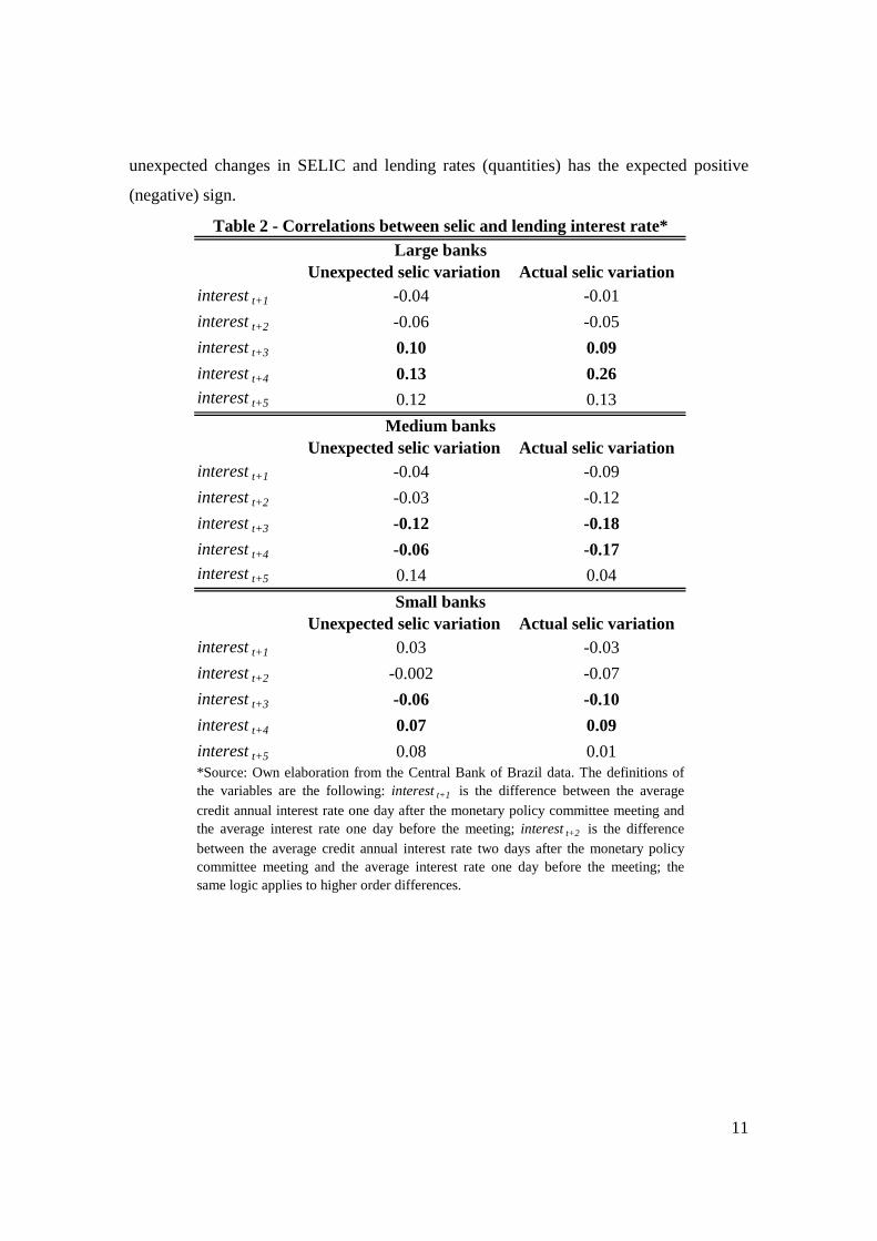
Tables 2 and 3 have pairwise correlations between changes in lending interest rate

and Selic (unexpected and actual), and changes in new loans and Selic (unexpected and

actual). Correlations suggest that it takes two days for changes in the basic rate to affect

lending rates and quantities: three and four days after the meeting the correlation between

-3

-2

-1

0

1

2

3

4

% y

ear

year-month

Figure 2: Actual x Unexpected changes in selic rate

Actual selic rate changes Unexpected selic rate changes

11

unexpected changes in SELIC and lending rates (quantities) has the expected positive

(negative) sign.

Unexpected selic variation Actual selic variationinterest t+1 -0.04 -0.01interest t+2 -0.06 -0.05interest t+3 0.10 0.09interest t+4 0.13 0.26interest t+5 0.12 0.13

Unexpected selic variation Actual selic variationinterest t+1 -0.04 -0.09interest t+2 -0.03 -0.12interest t+3 -0.12 -0.18interest t+4 -0.06 -0.17interest t+5 0.14 0.04

Unexpected selic variation Actual selic variationinterest t+1 0.03 -0.03interest t+2 -0.002 -0.07interest t+3 -0.06 -0.10interest t+4 0.07 0.09interest t+5 0.08 0.01*Source: Own elaboration from the Central Bank of Brazil data. The definitions ofthe variables are the following: interest t+1 is the difference between the averagecredit annual interest rate one day after the monetary policy committee meeting andthe average interest rate one day before the meeting; interest t+2 is the differencebetween the average credit annual interest rate two days after the monetary policycommittee meeting and the average interest rate one day before the meeting; thesame logic applies to higher order differences.

Table 2 - Correlations between selic and lending interest rate*Large banks

Medium banks

Small banks

12

Following the literature, we decompose the impact of monetary according to bank

size, and different categories have distinct funding profiles. Consider the size taxonomy

of figure 1. Table 4 shows deposits as a proportion of total liabilities for the three bank

size categories (large, medium and small).

Unexpected selic variation Actual selic variationnew_loans t+1 0.07 -0.15new_loans t+2 0.061 -0.09new_loans t+3 -0.13 -0.19new_loans t+4 -0.11 -0.31new_loans t+5 0.14 -0.02

Unexpected selic variation Actual selic variationnew_loans t+1 0.04 -0.11new_loans t+2 0.07 -0.11new_loans t+3 -0.02 -0.11new_loans t+4 -0.11 -0.31new_loans t+5 0.17 0.02

Unexpected selic variation Actual selic variationnew_loans t+1 -0.05 -0.17new_loans t+2 0.01 -0.15new_loans t+3 -0.07 -0.10new_loans t+4 -0.07 -0.24new_loans t+5 0.17 0.01

*Source: Own elaboration from the Central Bank of Brazil data. The definitions ofthe variables are the following: new_loans t+1 is the difference between the averagevolume of new loans one day after the monetary policy committee meeting and theaverage volume of new loans one day before the meeting; new_loans t+2 is thedifference between the average volume of new loans two days after the monetarypolicy committee meeting and the average volume of new loans one day before themeeting; the same logic applies to higher order differences.

Table 3 - Correlations between selic and new loans*Large banks

Medium banks

Small banks

13

Clear differences in funding strategies operation emerge. Large banks have the

highest percentage of their liability as deposits. Nevertheless, smaller banks have more

deposits than medium-sized banks. This is true for both sub-categories of deposits (time

and demand), but demand deposits are only relevant for large banks. Savings deposits

monotonically decrease with size.

Some of the facts in table 4 are unsurprising. Banks must have branches all over

the country in order to be able to compete for the demand and saving deposits. The time

deposits market is segmented between large denomination CDs and the “retail” market

for individuals. Small and medium size banks are able to get funding in the wholesale

CDs market.

III. Empirical Strategy

Identifying the banks’ lending reactions is akin to the standard problem of

estimating demand and supply relations in microeconometrics. The bank lending channel

refers to the supply side of the credit market, but we typically observe only equilibrium

values. Following a monetary policy shock, it is conceivable that not only the supply of

Total deposits/liabilityDemand deposits/liability Time deposits/liabilitySaving deposits/liabilityaverage 45.7 8.1 23.4 14.2median 45.6 8.9 22.0 12.4minimum 25.8 2.9 3.2 1.2maximum 74.7 13.0 43.6 31.3

Total deposits/liabilityDemand deposits/liability Time deposits/liabilitySaving deposits/liabilityaverage 20.7 2.5 14 4.6median 18.1 0.7 11 0minimum 0 0 0 0maximum 65.2 9 38 29.1

Total deposits/liabilityDemand deposits/liability Time deposits/liabilitySaving deposits/liabilityaverage 33.8 3.5 29 1.2median 25.5 0.5 20 0minimum 0 0 0 0maximum 98.1 67 98 37.3

*Source: Own elaboration from banks' balance sheet accounts (Cosif, Central Bank of Brazil)

Table 4: Deposit funding by bank's size - % of total liability*Large banks

Medium banks

Small banks

14

credit shifts, but also demand for credit, a problem first recognized by Kashyap and Stein

(1994).

Existing empirical literature has used bank characteristics to isolate demand

factors (Kashyap and Stein (2000), Arena et al (2007)). The key identifying assumption is

that banks differ in their abilities to substitute away from deposits. Furthermore,

observable characteristics determine the ability to move to and from deposits. In this

case, one may interpret different reactions to monetary policy as evidence of the bank

lending channel. Typically, one assumes that larger, more liquid and foreign owned (in

emerging countries) banks are better equipped to move to and from deposits. The

theoretical motivation behind these assumptions is as follows. The presence of deposit

insurance makes deposits free of informational asymmetries, thereby becoming the

cheapest and more stable way to fund bank credit operations. When forced to raise

equity, long-term debt and short-term wholesale debt, banks have to pay dearly for

informational asymmetries and non-contractibilities. In this context, larger banks, perhaps

because of too-big-to--fail effect or because they are easier to monitor, pay less when

substituting away from deposits to these more expensive instruments (see Kashyap and

Stein (2000) and Stein (1998)). The same would apply for foreign banks in emerging

countries. Liquidity also matters because, if banks have very liquid instruments in the

asset part of the balance sheet, they may sell position when facing funding shortage.

Finally, banks follow distinct strategies for funding. In Brazil, as Table 4 shows, larger

banks have a stronger reliance on deposits than smaller banks, although the industry’s as

a whole relies little on deposits in an international comparison.10

Regardless of the empirical validity of such theoretical arguments, banks with

characteristics serve different clientele. In this case, equilibrium reaction to monetary

policy may differ for demand reasons: different borrowers may react differently to

monetary policy shocks. For example, middle-market banks specialize in receivables’

discounting for Small and Medium Enterprises (SMEs). Large universal banks, in

addition to discounting, do short and medium term working capital loans for larger firms.

It is quite conceivable that large firms will reduce their working capital demand in

10 Among Latin American countries, the Brazilian banking system has the lowest Deposits-to-Liabilities ratio, 41%. The average is 65%. We kindly thank Arturo Galindo for pointing this out and sending out the data on different Latin American countries.

15

response to monetary tightening, but SMEs will not cut so fast their demand for

discounting. Furthermore, consumer credit is highly concentrated in larger banks, and

consumption and investment may react very differently to monetary policy.

In contrast with the literature, our main identification strategy is data-driven. A

well established fact in monetary economics is that output and inflation are only slowly

affected by the traditional monetary policy mechanism (see Christiano et al (1999),

among many others11). In the short run, consumption and investment decisions have some

inertia. Since monetary policy affects banks’ marginal cost immediately for several

products, credit supply should react faster to monetary policy than credit demand. Using

daily data and focusing on few days before and after the monetary policy committee

meeting, we are confident we are recovering only systematic supply shifts. In addition to

high frequency, we have information about flows, i.e., new loans. This is crucial for our

strategy to be successful because stocks hardly move much in the very short-run. Another

advantage vis-à-vis the literature, we have data on interest rate, which is useful to

corroborate that we capture supply shocks: supply and demand shocks to monetary policy

have similar implications for quantities, but opposite implications for interest rates.

Finally, we also follow the literature and decompose the response to monetary policy

according to bank characteristics, i.e., size, ownership and liquidity.

In the event study, we compare the amount of new loans issued and interest rates

charged on a few days before and after the monetary policy committee meeting to set a

new target for the basic interest rate. We use only the surprise of the announcement, i.e.,

the difference between the median expected change in the basic interest rate (day before

the meeting) and the actual change.12 In doing so, we mitigate the possibility that most

effects of policy announcement may have occurred way before the meeting.

We estimate the following equations:

11 The famous expression coined by Friedman [1972] is that monetary policy works with “long and variable lags.” 12 As a robustness test we used the actual interest rate changes too. Results are available upon request.

16

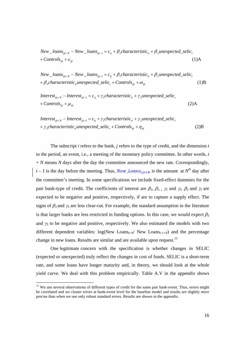
The subscript i refers to the bank, j refers to the type of credit, and the dimension t

to the period, an event, i.e., a meeting of the monetary policy committee. In other words, t

+ N means N days after the day the committee announced the new rate. Correspondingly,

t – 1 is the day before the meeting. Thus, _ is the amount at Nth day after

the committee’s meeting. In some specifications we include fixed-effect dummies for the

pair bank-type of credit. The coefficients of interest are β2, β3 , γ2 and γ3. β2 and γ2 are

expected to be negative and positive, respectively, if are to capture a supply effect. The

signs of β3 and γ3 are less clear-cut. For example, the standard assumption in the literature

is that larger banks are less restricted in funding options. In this case, we would expect β3

and γ3 to be negative and positive, respectively. We also estimated the models with two

different dependent variables: log(New Loanst+N/ New Loanst-1+N) and the percentage

change in new loans. Results are similar and are available upon request.13

One legitimate concern with the specification is whether changes in SELIC

(expected or unexpected) truly reflect the changes in cost of funds. SELIC is a short-term

rate, and some loans have longer maturity and, in theory, we should look at the whole

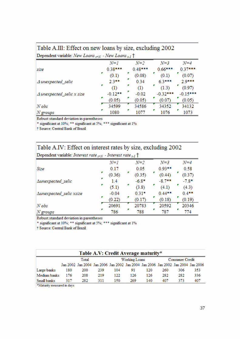
yield curve. We deal with this problem empirically. Table A.V in the appendix shows

13 We use several observations of different types of credit for the same pair bank-event. Thus, errors might be correlated and we cluster errors at bank-event level for the baseline model and results are slightly more precise than when we use only robust standard errors. Results are shown in the appendix.

(1)B

__

(1)A

__

3

211

211

ijtijttit

titijijtNijt

ijtijt

titijijtNijt

Controls_selicunexpectedsticcharacteri

_selicunexpectedsticcharactericloansNewloansNew

Controls

_selicunexpectedsticcharactericloansNewloansNew

ωβ

ββ

ε

ββ

+++

++=−

++

++=−

−+

−+

(2)B

(2)A

3

211

211

ijtijttit

titijijtNijt

ijtijt

titijijtNijt

Controls_selicunexpectedsticcharacteri

_selicunexpectedsticcharactericInterestInterest

Controls

_selicunexpectedsticcharactericInterestInterest

ηγ

γγ

μ

γγ

+++

++=−

++

++=−

−+

−+

17

two things. First, the average maturity of loans in Brazil is short: 7 months. Then, short-

term rates seem appropriate. Second, there is heterogeneity in maturity among different

types of loans. So, if estimates are not sensitive to the type of loan considered, SELIC is

not a bad measure of cost of funds.

IV. Results

IV.A. General effects of monetary policy

IV.A.1 Main estimates

Tables 5 and 6 show the results for (1)A and (2)A, i.e., the models without any

decomposition:

N=1 N=2 N=3 N=4Δ unexpected_selic .17*** .015 -.29*** -.11***

(.048) (.032) (.048) (.025)N obs 45532 45480 45255 45030N groups 1090 1087 1085 1083

† Source: Central Bank of Brazil

Table 5: Effect on new loans without decompositionDependent variable: New Loans t+N - New Loans t-1 †

Robust standard deviation in parentheses* significant at 10%; ** significant at 5%; *** significant at 1%

N=1 N=2 N=3 N=4Δ unexpected_selic -.64*** -.69*** .63*** 1.4***

(.2) (.19) (.18) (.18)N obs 27060 27097 27022 26633N groups 810 812 811 803


Table 6: Effect on interest rates without decompositionDependent variable: Interest rate t+N - Interest rate t-1 †


18

The results show that unexpected changes in the SELIC rate have a negative and

statistical significant effect on new loans, and a positive and statistical significant effect

on lending interest rate on the third and fourth days after the committee’s meeting. In

days 1 and 2, results are reversed. We prefer results for days 3 and 4 for four reasons.

First, they are more consistent than results for days 1 and 2. In fact, day 2’s the impact on

quantity is zero. Second, banks may hesitate to move on the very first days, to avoid

moving alone. This is yet more important for small banks, which may act as followers. In

fact, when we decompose observations by size, we see that results for days 1 and 2 for

larger banks are inconsistent for prices and quantities (see tables 9 and 10 below). Third,

there is a delay between the contract date and the fund release date. For example, the

contract date could be one day after the meeting, but the actual release of the fund could

be two or three days after. The same kind of effect could affect the new loans one and

two days after the meeting: in this case at least part of the loans actually refers to the day

of the meeting (or even prior), which is not affected by the new information about basic

interest rate. Last, but not least, results for days 3 and 4 have theoretical support: they

represent a supply shift. Even if they were consistent, it would be hard to interpret results

for days 1 and 2 because they are compatible with demand, not supply, and demand

should not respond this quickly. Thus, throughout the discussion, we focus on days 3 and

4.

In quantitative terms, an unexpected increase of the Selic rate of 1% per year

implies a drop14 of average daily new loans of R$290 thousand (US$ 107 thousand, about

11% of the average value of the new loans in the sample). Industry wide this means an

impact of R$57.7 million (US$ 21.3 million, approximately 2.7% of the average value of

the industry new loans in the sample). 15

The effect of SELIC on credit interest rate is positive and statistically significant

in windows 3 and 4. The estimated pass-through in the 3-days window is less than one,

which means that not all Selic’s variation is passed on credit interest rate. This stickiness

is compatible with market power (Panzar and Rosse (1987)) or with adverse selection in

14 These calculations use the 3-days window results. 15We use several observations of several different types of credit for the same pair bank-event. Thus, errors might be correlated and we cluster errors at bank-event level for the baseline model and results are slightly more precise than when we use only robust standard errors. Results are shown in the appendix.

19

credit markets as in Stiglitz and Weiss (1981). The signs and magnitudes of our estimated

responses to SELIC for the 3 and 4-days windows are compatible with supply but not

demand shifts, corroborating our identification strategy.

IV.A.2 Robustness checks

Figure 1 shows that our sample contains only a few large banks. By equally

weighting, the documented differences come mostly from differences between medium

and small ones. To prove our results, we weight observations by bank size. Results,

which are similar, are in tables A.I and A.II of the appendix.

Figure 2 shows that our sample contains several events in 2002, a year of

economic turmoil in Brazil. Therefore, our results may be driven by crisis periods. We re-

estimate the model excluding all events from 2002. Results, which are similar, are in

tables A.III and A.IV of the appendix.

Another important issue concerns the possibility of hoarding. If announcements

are made at pre-announced dates, lenders (or banks) may hoard loan applications until the

uncertainty is uncovered. Two comments are in place. First, hoarding applies only to

quantities, not interest rates. Second, we take steps to address the possibility that

hoarding mechanically produces the results for quantities. If hoarding is in fact relevant

empirically, we should observe that new loan concessions should be lower in the days

immediately preceding the COPOM meetings than, say, 7 to 10 days before the meeting.

This is irrespective of whether SELIC rates surprise up or down. Table A.VI in the

appendix shows that this is not the case.

IV.B Size Decomposition

In this subsection we follow the literature and estimate models (1)B and (2)B

decomposing the impact of monetary policy according to bank size. The intuition is that

as larger banks have more collateral to offer, they probably will find easier to trade

deposits for other kind of debts. Furthermore, investors could be more willing to buy

shares of larger banks if they thought government saw them as too big to fail. We use the

20

log of assets as a measure of size. Tables 7 and 8 show the results for new loans and

interest rate, respectively16.

16 The results using size could be generated by the larger amount of medium and small banks in our sample. In order to deal with this possible problem we estimated the same model of this section including weights based on the sample average size of each bank. Results are showed in the tables A.I and A.II of the appendix. We can see that results are not qualitatively different from those of tables 6 and 7.

21

In line with our previous estimates, banks’ reactions to changes in monetary

policy are again compatible with a supply response: they increase lending interest rates

and contract new loans after a monetary policy contraction.

Results on the interaction term are in sharp contrast with existing literature. If

large banks were better equipped in substituting away from deposits, they should respond

less strongly to changes in monetary policy. In fact, they respond more strongly. Using

estimates in tables 7 and 8, tables 9 and 10 show the average response for the three

groups of banks: small, medium and large sized. In general, small banks do not respond

to shocks in monetary policy. On the other hand, among large banks a one percentage-

point unexpected increase in the SELIC rate causes an average daily reduction of R$1.24

million (US$ 459 thousand), which means an average aggregate daily reduction of

R$13.6 million (US$ 5.03 million, approximated 8.8% of the average value of the large

banks new loans in the sample). Accordingly, interest rates charged by small banks is

insensitive to unexpected changes in monetary policy and a one percentage-point

unexpected increase in the SELIC rate causes a increase of 2.13 percentage points in the

interest rate charged by large banks17.

17 Figure 2 shows that five events of unexpected changes in Selic occurred in 2002, a year of economic crisis in Brazil. To ensure that results are not confined to crisis period, we re-estimated the model of this section excluding 2002. Tables A.III and A.IV of the appendix have the results, which are qualitatively similar to those in tables 6 and 7.

22

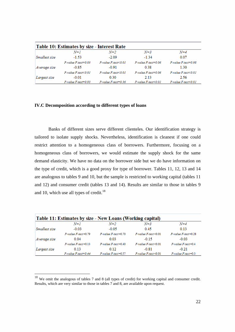
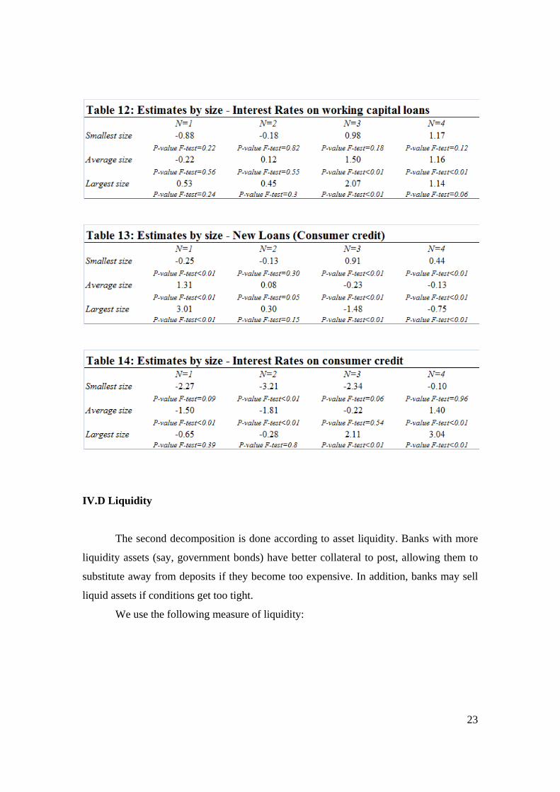
IV.C Decomposition according to different types of loans

Banks of different sizes serve different clienteles. Our identification strategy is

tailored to isolate supply shocks. Nevertheless, identification is cleanest if one could

restrict attention to a homogeneous class of borrowers. Furthermore, focusing on a

homogeneous class of borrowers, we would estimate the supply shock for the same

demand elasticity. We have no data on the borrower side but we do have information on

the type of credit, which is a good proxy for type of borrower. Tables 11, 12, 13 and 14

are analogous to tables 9 and 10, but the sample is restricted to working capital (tables 11

and 12) and consumer credit (tables 13 and 14). Results are similar to those in tables 9

and 10, which use all types of credit.18

18 We omit the analogous of tables 7 and 8 (all types of credit) for working capital and consumer credit. Results, which are very similar to those in tables 7 and 8, are available upon request.

23

IV.D Liquidity

The second decomposition is done according to asset liquidity. Banks with more

liquidity assets (say, government bonds) have better collateral to post, allowing them to

substitute away from deposits if they become too expensive. In addition, banks may sell

liquid assets if conditions get too tight.

We use the following measure of liquidity:

itit AssetsTotalliquidity =

24

Tables 15 and 16 present the results.

Contrary to theoretical arguments, estimates show that liquidity does not appear to

influence the transmission of monetary policy through the bank lending channel.

25

IV.E Deposits and Earmarked Funds

The credit channel of monetary policy operates mainly through its impact on the

cost of funds to banks. Deposits, a form of short-term debt, are immediately affected by

changes in the basic rate. Thus, one should conjecture that the impact of monetary policy

depends on the proportion of deposits different banks hold in their liabilities. In fact, as

Table 4 shows, larger banks rely more on demand deposits than smaller ones. Because of

that, results in subsection IV.B may be due to different liability composition (see

subsection IV.F for further evidence). Tables 17 and 18 test this conjecture.

N=1 N=2 N=3 N=4%demand deposits -.016 .31 .065 -.28

(.35) (.3) (.32) (.28)Δ unexpected_selic .1*** .00072 -.21*** -.088***

(.035) (.024) (.035) (.02)Δ unexpected_selic x %demand deposits 1.3*** .28 -1.5*** -.39**

(.43) (.26) (.44) (.2)N obs 45442 45404 45181 44956N groups 1090 1087 1085 1083


Table 17: Effect on new loans by demand depositsDependent variable: New Loans t+N - New Loans t-1 †


26

In line with the conjecture, Tables 17 and 18 show that banks rely more on

deposits for their funding respond more to changes in monetary policy. This is true for

both on interest rates and loan concessions at the same three and four day window. Small

and large banks differ in their funding strategy. Then, it is important to check whether

results in tables 8 and 9 are robust to controlling for difference in funding strategy (see

tables 23 and 24 below).

Also on the liability side, banks receive funding from the government through

some programs. BNDES earmarked for working capital to small and medium-sized firms

is the largest component of this kind of fund. These loans have variable but regulated

rates and, by construction, should respond less to shocks on monetary policy. Tables 19

and 20 have the estimates of the models (1)B and (2)B decomposed by BNDES funding

as a percentage liabilities.

N=1 N=2 N=3 N=4%demand deposits -.66 2.1 1.4 -6.2*

(3.2) (3.8) (3.2) (3.3)Δ unexpected_selic -.69** -.61*** .55** 1***

(.27) (.24) (.24) (.22)Δ unexpected_selic x %demand deposits 1.1 -1.4 1.3 5.4***

(2.1) (1.6) (1.7) (1.8)N obs 27006 27048 26976 26584N groups 810 811 811 803


Table 18: Effect on interest rates by demand depositsDependent variable: Interest rate t+N - Interest rate t-1 †


27

In line with expectations, banks with a large share of earmarked BNDES funding

are less sensitive to changes in monetary policy. Again, banks differ in their reliance on

earmarked funds. Thus, as previously emphasized, it is important to check whether

results in tables 8 and 9 are robust to controlling for difference in earmarked funding (see

tables 23 and 24 below).

IV.E Ownership

N=1 N=2 N=3 N=4%earmarked funds -.018 -.075 -.24 -.21

(.22) (.22) (.22) (.2)Δ unexpected_selic .18*** .015 -.31*** -.12***

(.052) (.034) (.051) (.026)Δ unexpected_selic x %earmarked funds -.16* .0059 .31*** .14***

(.091) (.063) (.094) (.05)N obs 45442 45404 45181 44956N groups 1090 1087 1085 1083


Table 19: Effect on new loans by earmarked fundsDependent variable: New Loans t+N - New Loans t-1 †


N=1 N=2 N=3 N=4%earmarked funds .38 2.4 2.8 3.6

(2.5) (2.3) (2.4) (2.3)Δ unexpected_selic -.65*** -.84*** .55*** 1.4***

(.21) (.21) (.21) (.19)Δ unexpected_selic x %earmarked funds .4 2.8*** 1.4 .36

(1.2) (1) (1.1) (1)N obs 27006 27048 26976 26584N groups 810 811 811 803


Table 20: Effect on interest rates by earmarked fundsDependent variable: Interest rate t+N - Interest rate t-1 †


28

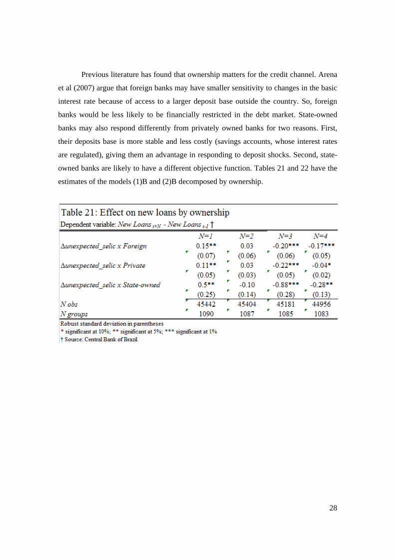
Previous literature has found that ownership matters for the credit channel. Arena

et al (2007) argue that foreign banks may have smaller sensitivity to changes in the basic

interest rate because of access to a larger deposit base outside the country. So, foreign

banks would be less likely to be financially restricted in the debt market. State-owned

banks may also respond differently from privately owned banks for two reasons. First,

their deposits base is more stable and less costly (savings accounts, whose interest rates

are regulated), giving them an advantage in responding to deposit shocks. Second, state-

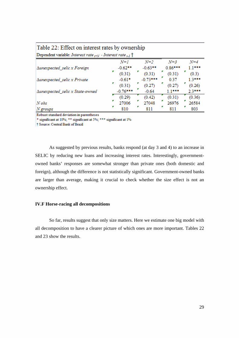
owned banks are likely to have a different objective function. Tables 21 and 22 have the

estimates of the models (1)B and (2)B decomposed by ownership.

29

As suggested by previous results, banks respond (at day 3 and 4) to an increase in

SELIC by reducing new loans and increasing interest rates. Interestingly, government-

owned banks’ responses are somewhat stronger than private ones (both domestic and

foreign), although the difference is not statistically significant. Government-owned banks

are larger than average, making it crucial to check whether the size effect is not an

ownership effect.

IV.F Horse-racing all decompositions

So far, results suggest that only size matters. Here we estimate one big model with

all decomposition to have a clearer picture of which ones are more important. Tables 22

and 23 show the results.

31

When we horse-race all explanations, results are somewhat similar to those we get

when estimating the models separately. We find that a stronger response by larger banks

(reduce more new loans and increase more the interest rate). Banks whose funding rely

more on deposits increase their interest rates more, as expected, but we find no results on

quantities. Thus, we do not find these results conclusive. A higher proportion of

earmarked funds is associated with a damped response in quantities, but no response in

32

interest rate. This is precisely as expected: earmarked funds are passed on with regulated

rates. Then, prices should not respond much.

V. Conclusion

We studied the monetary policy transmission mechanism that works through bank

credit in Brazil: the bank lending channel. We had access to a unique data set that include

all bank credit concessions (above a threshold) in Brazil, both to firms and people. The

data include the loan amount and the interest rate charged. We use the daily frequency of

the new loans and interest rate information to identify bank credit supply responses to

monetary policy shocks (unexpected basic interest rate changes) in a cleaner way than in

the previous literature.

In contrast to the existing empirical literature for other countries, in Brazil, larger

banks respond more to shocks in monetary policy than smaller ones. We do not interpret

this result as evidence contrary to the theoretical mechanism behind the bank lending

channel. The empirical literature typically uses US data (Kashyap, Stein and Wilcox

(1993), Kashyap, Stein (2000)). The assumption – reasonable for the US - is that

informational asymmetries and moral hazard problems plague smaller banks more than

large ones. In Brazil the assumption is much less obviously true.

Our results have potentially important implications for the conduct of monetary

policy in Brazil. The impact of changes in the basic interest rate (SELIC) is transmitted

more strongly by larger banks, which hold the largest share of loans in the economy,

increasing the power of monetary policy. Furthermore, market structure has been

changing. In particular, consolidation has increased the size of a typical bank. Our results

suggest that the power of the monetary policy through the credit channel will increase

overtime.

33

References

Stein, Jeremy, “An adverse-selection model of bank asset and liability management with

implications for monetary policy,” The Rand Journal of Economics, Vol. 29, pp. 466-

486.

Arena, Marco, Carmen Reinhart and Francisco Vasquez, “The lending channel in

emerging economies: are foreign banks different?”, IMF working paper, WP/07/48, Feb.,

2007.

Bernanke, Ben and Alan Blinder, “Credit, money and aggregate demand,” American

Economic Review, Vol. 78, pp. 435-9, 1988.

Bernanke, Ben and Alan Blinder, “The Federal Funds rate and the channels of monetary

policy transmission”, American Economic Review, Vol. 82, pp. 901-921, 1992.

Bernanke, Ben and Mark Gertler, “Agency costs, net worth and business fluctuations,”

American Economic Review, Vol. 79, pp. 14-31, 1989.

Bernanke, Ben, Mark Gertler and S. Gilchrist, The financial accelerator in a quantitative

business cycle framework, in J. B. Taylor e M. Woodford (eds.) Handbook of

Macroeconomics, North-Holland, 2000.

Berger, Allen, Nathan Miller, Mitchell Petersen, Raghuram Rajan, and Jeremy Stein

“Does function follow organizational form? Evidence from the lending practices of large

and small banks” Journal of Financial Economics, Vol. 75, pp. 237-269, 2005.

BIS, “Monetary policy framework and central banks operations”, April 2008.

34

Christiano, Laurence, Martin Eichenbaum and Charles Evans, “Monetary policy shocks:

what have we learned and to what end?”, Handbook of Macroeconomics, Vol. 1, Part A,

pp. 65-148, 1999.

Costa, Ana Carla A. and Márcio I. Nakane, “Revisitando a metodologia de decomposição

do spread bancário no Brasil”, in: XXVI Encontro brasileiro de econometria, João

Pessoa, 2004.

Costa, Ana Carla A. and Márcio I. Nakane, “Spread bancário: os problemas da

comparação internacional”, (pdf), 2005.

Fachada, Pedro, Figueiredo, Luiz Fernando and Lundberg, Eduardo, “Sistema judicial e

mercado de crédito no Brasil”, Notas técnicas do Banco Central do Brasil, No. 35, May,

2003.

Friedman, Milton (1972), ‘Have Monetary Policies Failed?’, American Economic Review (Papers and Proceedings), 62, 11–18.

Gelos, Gaston, “Banking spreads in latin america”, IMF working paper, WP/06/44,Feb.,

2006.

Kashyap, Anil and Jeremy Stein, “The impact of monetary policy on bank balance

sheets”, NBER working paper series No. 4821, August, 1994.

Kashyap, Anil and Jeremy Stein, “What do a million of observations on banks say about

the transmission of monetary policy?”, The American Economic Review, Vol. 90, pp.

407-428, Jun., 2000.

Kashyap, Anil, Jeremy Stein and David Wilcox, “Monetary policy and credit conditions:

evidence from the composition of external finance”, American Economic Review, Vol.

83, No. 1, pp. 78-98, Mar., 1993.

35

N. Kiyotaki and J. Moore, “Credit Cycles,” Journal of Political Economy, Vol. 105. pp.

211-48, 1997.

Nakane, Márcio, Fabiana Rocha and Tony Takeda “The reaction of banking lending to

monetary policy in Brazil”, Revista Brasileira de Economia, Vol. 50, pp. 107–126, 2005.

Panzar, John and James Rosse, “Testing for the “monopoly” solution,” Journal of

Industrial Organization, Vol. 35, pp. 34-

Stiglitz, J. E., A. Weiss. “Credit rationing in markets with imperfect information,”

American Economic Review, Vol. 71, 1981.

Appendix

Departamento de Economia PUC-Rio

Pontifícia Universidade Católica do Rio de Janeiro Rua Marques de Sâo Vicente 225 - Rio de Janeiro 22453-900, RJ

Tel.(21) 35271078 Fax (21) 35271084 www.econ.puc-rio.br [email protected]

no. 574 identifying the bank lending channel in brazil

Documents