No Pain, No Gain:

The Effects of Exports on Sickness, Injury, and Effort

David Hummels, Purdue University and NBER

Jakob Munch, University of Copenhagen and IZA

Chong Xiang, Purdue University

November 2016

Abstract: Health is an important contributor to our well-being, but we do not fully understand how to quantify this contribution, or how demand shocks affect health. We combine Danish data on individuals’ health with Danish matched worker-firm data. We find that when firm exports rise for exogenous reasons: 1. Women have higher sickness rates. For example, a 10% exogenous increase in exports increases women’s rates of depression by 2.5%, and hospitalizations due to heart attacks or strokes by 15%. 2. Both men and women have higher injury rates, both overall and correcting for hours worked; and 3. Both men and women work longer hours and take fewer sick-leave days. We then develop a novel framework to calculate the marginal disutility of any non-fatal disease, and to aggregate across multiple types of sickness and injury to compute the total utility loss. The ex-ante utility loss due to higher sickness rates is one fifth of the wage gain from rising exports for the average man, and over one half for the average woman. Our marginal disutility estimates suggest that ex post, those who actually get injured or sick suffer large utility losses; e.g. exceeding 3 million Danish Kroner for a woman who is hospitalized due to a heart attack or stroke. JEL: I1, F1, J2 and F6. Acknowledgements: We thank the The Danish Council for Independent Research | Social Sciences for funding. For helpful comments we thank Osea Giuntella, Nils Gottfries and seminar participants at NHH Bergen, University of Oslo, University of Oxford, ESWC Montreal, University of Lund, Singapore Management University, University College Dublin, Copenhagen Business School, Aarhus University, IFN Stockholm, University of Chicago, Uppsala University and University of Oxford Trade and Health Workshop.

1

1. Introduction

Health is an important contributor to our well-being, but we do not yet fully understand how

health responds to demand shocks, an important question that is of interest for academic research, the

general public and policy makers. An expansion of demand likely raises income, and many studies

show that higher income or wealth leads to better health (e.g. Marmot et al. 1991, Smith 1999, and

Sullivan and von Wachter 2009). In contrast, Ruhm (2000)’s finding that the U.S. mortality rate is pro-

cyclical suggests a competing channel: rising demand may lead to higher health risks, due to increased

stress and efforts or reduced leisure. However, tight identification of this channel remains challenging.

Stevens, Miller, Page and Filipski (2015), for example, argue that Ruhm (2000)’s result for mortality is

driven by staffing changes at nursing homes.1

Nor do we fully understand how to quantify the contribution of health to our well-being. While

estimates for the marginal disutility of mortality and injury, or VSLI (value of a statistical life/injury),

have been well-established (e.g. Viscusi 1993) and widely used by U.S. regulatory agencies (e.g.

Viscusi and Aldy 2003), similar estimates for non-fatal diseases remain elusive. For example, Jones

and Klenow (2016)’s well-being index incorporates mortality but leaves out morbidity.

In this paper we tackle both questions. Our matched worker-firm data allows us to show that

within job-spells, the hazard rates of worker-level stress, injury, and illness increase in response to

exogenous rises of export activities within the workers’ employers, a source of exogenous shocks to

work demand. We also find that this demand increase can be met by inducing workers to expand hours

and increase work intensity, a potentially important adjustment mechanism that has been largely

overlooked in the literature on globalization and labor markets (e.g. Verhoogen 2008, Autor, Dorn and

Hanson 2013, and Hummels, Jørgensen, Munch and Xiang 2014, or HJMX 2014)2. Taking this one

1See also Lindo (2013), Tekin, McClellan and Minyard (2013), Ruhm (2013) and Coile, Levine and McKnight (2014). 2 For recent surveys see Goldberg and Pavcnik (2007), Harrison, McLaren and McMillan (2011), and Hummels, Munch and Xiang (2016).

2

step further, we develop a novel framework to calculate the aggregate losses in well-being, or ex-ante

utility losses, that result from higher rates of non-fatal injury and illness. This framework also allows us

to calculate the marginal disutility of any non-fatal disease, which corresponds to ex post utility losses

for those who actually get sick. Our utility-loss calculations suggest that, in the spirit of Rosen (1986),

some of the wage gains from rising exports may reflect compensating differential. Recent studies have

examined the implications of health status for GDP (e.g. Murphy and Topel 2003, Becker, Philipson

and Soares 2005), macro-economic fluctuations (e.g. Egan, Mulligan and Philipson 2013) and

economic growth (e.g. Jones 2016) by focusing on mortality. Our framework may help broaden the

scope of the inquiry to also examine non-fatal injuries and diseases.

We draw on Danish administrative data that match the population of Danish workers to the

universe of private-sector Danish firms. For each firm, we have detailed information on its

characteristics, including trade activity. For each individual we observe socio-economic characteristics

and rich details about every interaction between every individual and the Danish healthcare system. For

example, we observe the universe of prescription drug purchases made by every individual in

Denmark, plus the date (by week), total cost and the type of drug (by 4-digit classification) of every

purchase. We have similar information for doctor visits and hospitalization. This rich data on

individuals’ health is available to us because Danish health care is free and universal, and every

individual has access to health care, regardless of income and employment status. This distinguishes

our work from previous research on health and labor market using U.S. data, where workers’ access to

health care is correlated with income and employment status.3

To motivate our estimation, we consider a framework where workers bargain with their

employer. Each worker chooses the optimal effort level by equalizing the marginal benefit of effort,

determined through bargaining, with the marginal cost of effort, due to hazards of stress and sickness.

3 See, e.g., Currie and Madrian (1999) for a survey.

3

When exports rise exogenously, demand for the firm’s output rises, and so the marginal benefit of

efforts increases. As a result, workers’ efforts increase, and so do their rates of stress and sickness. For

specific disease types we focus on job injury and heart attacks and strokes, because stress and efforts

are both risk factors for them according to medical research.4

We face several significant challenges in taking our hypotheses to the data. One, individuals’

health is affected by many idiosyncratic and time-invariant factors, such as early-childhood and pre-

natal development.5 Two, individual workers’ stress and efforts are very hard to observe in the data.

Three, exports are endogenous. A firm may export a lot because it uses superior technology and good

management practices, which, in turn, may reduce its employees’ injury and sickness rates.

The comprehensive and panel structure of our Danish data allow us to deal with the first two

issues. First, we consistently track each worker and each firm over time and so we are able to condition

on job-spell fixed effects; i.e. the source of our variation is the change over time within a given worker-

firm relationship. Second, a salient feature of our sample is that exports and output per worker have

strong positive correlation at the firm level, and the richness of our data allows us to directly measure

both stress and efforts at the worker level. For stress we observe the universe of anti-depressant

purchases and visits to psychiatrists of every worker. For efforts we observe total hours worked,

including over-time, by individual workers, which is an indicator for the extensive margin of efforts.

This then allows us to construct hours-based injury rate for individual workers, an indicator for the

intensive margin of efforts. Following the literature (e.g. Ichino and Maggi 2000, Hesselius et al., 2009,

Ichino and Moretti 2009) we also use workers’ sick-leave days as an indicator for efforts.6 However,

4 e.g. Harkness et al., 2004, Virtanen et al. 2012, O’Reilly and Rosato 2013, Kivimaki and Kawachi 2015. The medical literature focuses on risk factors and correlation patterns, and does not relate injury and sickness rates and efforts to demand shocks. . 5 See, e.g. Case and Paxson 2008. Almond and Currie (2011) provide a recent survey. 6 Other measures for shirking/efforts include survey questions (e.g. Freeman, Kruse and Blasi, 2008) and outputs of individual workers at individual firms (e.g. Lazear 2000, Mas and Moretti 2009). The medical literature also uses the number of sick-leave days (e.g. Kivimaki et al, 2005), but, again, does not have information about what the workers do during sick-leave spells.

4

we can go one step further to distinguish between their “major” and “minor” sick-leave days because

we observe the universe of healthcare transactions. Major-leave sick days correspond to time off work

in which workers also access healthcare, see a doctor or buy prescription drugs, within a week. Minor

sick-leave days correspond to time off work in which workers do not access healthcare. We show that

major and minor sick days have different responses to exports.

To address the endogeneity of exports, we follow our previous work, HJMX 2014, and

construct instruments for exports. A key feature of firms’ exporting behavior in our data is that within

the same industry, otherwise similar firms sell different 6-digit products to different destination

countries.7 This allows us to construct instruments, transportation costs and importer demand shocks,

that are specific to a particular partner country x product x year, but whose impact varies across firms.

These instruments generate large exogenous firm-year variation in the exports, providing an excellent

source of identification for changing work intensity and health outcomes.

We find that rising exports lead to higher rates of injury, for both men and women, and

sickness, mainly for women. A 10% exogenous increase in exports increases women’s chance of severe

job injury by 6.35%, depression by 2.51%, the use of antithrombotic drugs by 7.70%, and

hospitalizations due to heart attacks or strokes by 15.01%. We also find that rising exports lead to

increased efforts. For the extensive margin, both men and women increase total hours (regular hours

plus over-time hours) as exports rise exogenously. For the intensive margin, the elasticity of hours with

respect to exports is smaller than the elasticity of injury rates, and workers have higher hours-based

injury rate. In addition, exports have non-linear effects on sick-leave days. Following modest export

shocks both men and women reduce major and minor sick-leave days, consistent with adjustment along

the extensive margin of efforts. Following large export shocks, workers experience more major sick-

leave days but no change in minor sick-leave days, consistent with the intensive margin. These results

7 As we show in our previous work, HJMX 2014, of the distribution of the number of firms exporting the same product to the same destination country, the median is 1 and the 90th percentile is 3.

5

are novel to the literature.

To quantify the effects of non-fatal diseases on well-being, we start from individuals deriving

expected utility (e.g. Ma and McGuire 1997, Cutler and Zeckhauser 2000) from one healthy state and

multiple sick states. Then by the logic of compensating variation, there exists a monetary compensation

that equates this expected utility to the utility level in the completely healthy state. This monetary

compensation quantifies the ex-ante utility loss due to risks of injury and sickness. However, it is hard

to compute the level of this monetary compensation, because the literature on the state dependence of

utility has not reached a consensus about how marginal utilities in healthy and sick states differ.8 We

take a different approach. Rather than focus on the level of monetary compensation, we compute how

it changes when a worker is subject to increased rates of sickness and injury. We first show that the

functional relationship between the monetary compensation and sickness rates is akin to a cost

function; namely, the utility loss is increasing and weakly convex with respect to individual sickness

rates. Building on this functional relationship, we show that we can carry out our computation using the

percentage changes of sickness rates in response to demand shocks, their share weights, and the

marginal disutility of one disease type. We obtain the first from our own estimation, the second using

healthcare expenditure shares, and the last for injury by following the estimation procedure of the VSLI

literature.

Our framework then allows us to calculate the ex-ante utility loss of the average worker, due to

higher rates of injury and multiple types of non-fatal illness. Relative to the wage gains from rising

exports, this loss is substantial, 20.04% for the average man and 53.50% for the average woman. These

results suggest that a substantial portion of the wage gains due to rising exports could be compensating

differential for higher risks of injury and sickness. In addition, the comparison between men’s and

8 It is negative (positive) state dependence if marginal utility in the healthy state is higher (lower) than in sick states. For example, Viscusi and Evans (1990) and Finkelstein, Luttmer and Notowidigdo (2013) report evidence for negative state dependence, Lillard and Weiss (1998), Edwards (2008) and Ameriks, Briggs, Caplin, Shapiro and Tonetti (2016) report positive state dependence, while Evans and Viscusi (1991) report no state dependence.

6

women’s ex-ante losses suggests that rising exports, or rising demand in general, leads to inequality in

health and well-being, complementing the literatures on gender wage inequality and globalization and

income inequality.9 We are also able to calculate the marginal disutility of any non-fatal disease, and

this represents the ex-post utility loss of those workers who actually get sick. These ex-post losses are

large, e.g. exceeding 3 million Danish Kroner for a woman who gets hospitalized due to a heart attack

or stroke (1 DKK is about 0.18 USD in our sample period). Given that the estimates of the VSLI

literature are widely used in policy making, we hope that our marginal-disutility estimates for non-fatal

diseases can be useful for policy analyses, too.

In economics, two approaches have produced estimates of utility losses from non-fatal diseases.

The first is based on estimates of the state dependence of utility (e.g. Viscusi and Evans 1990,

Finkelstein, Luttmer and Notowidigdo 2013), and the second uses surveys to ask people what

compensation they would like for hypothetical scenarios of injury and sickness (e.g. Viscusi 1993).

Both approaches cover specific disease types. Outside of economics, the DALY (Disability-Adjusted

Life Years) approach (e.g. Murray and Acharya 1997) covers many disease types by converting one

life year with diseases into fractions of disease-free life years using disease-specific discount factors.

These discount factors, however, are constructed from survey data (e.g. collected at World Health

Organization meetings) that reflect the “social preferences” of public-health and other government

officials.10 Our framework combines the strengths of these approaches, because we can calculate both

ex-ante and ex-post utility losses of any non-fatal disease, our calculations are based on economic data

reflecting people’s actual choices, and our framework accommodates positive, negative or no state

dependence.

Our work also speaks to the studies that examine the effects of mass layoffs and plant closures

9 One survey of the former literature is Altonji and Blank (1999), and one for the latter Goldberg and Pavcnik (2007). 10 A related approach, QALY (Quality-Adjusted Life Years), assigns utility scores to diseases, assuming that utility is cardinal and people are risk neutral. These utility scores are obtained through judgments by experts or surveys of consumers (e.g. Torrance 1986).

7

on mortality and hospitalization using panel data (e.g. Sullivan and von Wachter 2009, Browning and

Heinesen 2012),11 and those that examine the non-pecuniary effects of import competition (e.g. Autor,

Dorn, Hanson and Song 2014, McManus and Schaur 2015, Pierce and Schott 2016).12 Relative to

these studies we examine the effects of exports, explore a unique set of exogenous shocks that change

the competitive environment of firms, and study the micro channels through which these shocks affect

workers’ injury and sickness.

In what follows, section 2 describes our data. Section 3 provides a theoretical framework to

motivate our empirical specifications, and describes how we construct our instrument variables.

Section 4 presents our results for stress and depression, heart attacks and strokes, and related illness.

Section 5 shows our results for injury. Section 6 shows our results for efforts. Section 7 explores how

the effects of exports vary across occupations and presents the robustness exercises. Section 8 develops

our framework to calculate utility losses. Section 9 concludes.

2. Data

In this section we discuss the main features of our data and our variables for stress, efforts,

injury and illness. We report more details of data construction in the Appendix.

We start with Danish administrative data that matches workers to firms and the import and

export transactions of these firms. The data are annual, cover the period 1995-2006, and match the

population of Danish workers to the universe of private-sector Danish firms. Each firm’s trade

transactions are broken down by product, and origin and destination countries. The primary data

sources are the Firm Statistics Register, the Integrated Database for Labor Market Research (“IDA”),

11 See also Browning, Danø and Heinesen (2006), Eliason and Storie (2007, 2009), and Black, Devereaux and Salvanes (2012). Outside of economics the Framingham heart sample (e.g. Hubert et al. 1983) and the Whitehall sample (e.g. Bosma et al. 1997, Marmot et al. 1997) are two widely-used panel data sets. The former is slightly obese relative to the population, and the latter, civil servants in London. 12 See also Dix-Carneiro, Soares and Ulyssea (2015), Colantone, Crinò and Ogliari (2015) and Autor, Dorn and Hanson (2015).

8

the link between firms and workers (“FIDA”), and the Danish Foreign Trade Statistics Register. 13 Our

identification strategy, which we discuss in detail in sub-section 3.3, requires that we look at exporting

firms. We also focus on the sectors where firms export a large share of their output, and job-related

injury is not uncommon, in order to give our hypotheses a decent chance with data. These

considerations take us to our main sample of large manufacturing firms spanning 1995-2006 with

nearly 2 million worker-firm-year observations.14 Table 1 shows the summary statistics of log hourly

wage, experience, marital status and union status. These values are similar for our main sample as

compared with the samples of the Danish labor force, or the Danish labor force in manufacturing (see

Table A2).

Table 1 also shows that the firms in our sample are highly export oriented, with an average

export-to-sales ratio of 0.66. This implies that exports and output are likely to move together for a

given firm. Further, exports and output move more than employment. We calculate the absolute values

of the deviations from within-job-spell means for log export, log output, and log employment. On

average, export deviates from its job-spell mean by 0.275 log points, output by 0.143 log points, and

employment by 0.106 log points. As a result, changes in output per worker, a firm-level proxy for

efforts, are positively correlated with changes in exports. In Table 2 we show this correlation by

regressing log output per worker on exports, conditional on firm fixed effects and weighted by firm

size.15 In columns 1 and 2 we use log export, and in columns 3 and 4 we use the quartile dummies of

log exports. The coefficients of exports are always positive and highly significant, suggesting that the

co-movement of output per worker and exports is a main feature of our data. This also means that our

13 As we describe in HJMX 2014, Denmark is a good candidate for studying the effect of labor demand shocks on wages because it has one of the most flexible labor markets in the world. HJMX 2014 also has more detailed discussions of the worker-firm-trade data. 14 In Table A1 we list the export-to-sales ratio, injury rate and number of observations (by worker-firm) by sector for the exporting firms in the full sample for 2005. Agriculture-and-Fishing also has a high export-to-sales ratio and a high injury rate, but it has few worker-year observations relative to Manufacturing. 15 Firm size is employment in the first year the firm is observed in our data.

9

data is fertile ground for examining our hypothesis, namely, how worker-level stress, effort, injury and

illness respond to exogenous changes in exports.16

To study individual workers’ sickness and injury rates, we bring in additional administrative

datasets that contain comprehensive information about individuals’ health care utilization during 1995-

2009. We observe the universe of transactions for every person within the Danish healthcare system,

including doctors visits, prescription drug purchases, and hospitalization. Most of these data are

collected at weekly frequencies, and we aggregate them to annual frequencies to match our worker-

firm-trade data. In addition, these datasets are organized by the same worker identifiers as our worker-

firm data, allowing us to merge them. In the literature, a common concern for data on the utilization of

health care is that access to care could be correlated with individuals’ socio-economic conditions (e.g.

income and employment status), and that this correlation could contaminate the care-utilization data

(e.g. Currie and Madrian 1999). This concern is unlikely to be a main issue for us, because the Danish

healthcare system is almost entirely funded by the government, available to all Danish residents

regardless of employment status, and virtually free to all.17 Table 1 shows the summary statistics of our

worker-level variables.

For stress and depression we consider whether an individual has positive expenses on any anti-

depressant prescription drug, and whether an individual purchases anti-depressants or visits a

psychiatrist. Table 1 shows that women have a higher depression rate, 3.95%, than men, 2.43%,

consistent with medical research. Part of the reason could be that men and women have different

16 Our identification strategy is built on the rich variations of exports over time relative to the job-spell mean, and our instrument variables (see sub-section 3.3). We do not use policy changes for identification. This distinguishes our approach from the difference-in-difference estimation strategy, where there is little meaningful variation in the periods before and after the policy changes (Bertrand, Duflo and Mullainathan 2004). 17 There are two main exceptions. 1. Dental care is not covered. 2. Patients bear some co-payments for prescription-drug expenses. We do not consider dental visits in our study, and the prescription co-pays are small enough (roughly 0.13 percent of median income) that income constraints on access are unlikely to be binding.

10

responses to stressful events: women tend to feel sad and guilty while men feel restless and angry.18

This difference between men and women motivates our empirical specification, where we estimate the

differential impacts of exports on men vs. women.

Medical research suggests that depression is a risk factor for heart attacks and strokes,

insomnia, substance abuse and self harm. Therefore, we also consider these sickness conditions in our

analyses. Table 1 also shows that women have lower probability to be on drugs for heart attacks,

strokes, and other heart diseases, again consistent with medical research (e.g. Roger et al., 2012).

Stress and efforts are also risk factors for job injury. When a worker is injured on the job in

Denmark, they may file a petition for compensation with the National Board of Industrial Injuries

(NBII). If the job injuries are severe enough to cause permanent damages to the workers’ earning and

working abilities, then the workers are also eligible for a one-time, lump-sum monetary compensation

from the employers’ mandatory insurance. We observe all the petitions filed during 1995-2009, and the

final decision by NBII for each petition. To measure injury we consider whether an individual receives

positive monetary compensation from NBII.19 Table 1 shows that the mean injury rate is about 4 per

thousand in our sample, lower than in the U.S. data, probably because we only include severe injuries

while the U.S. data includes all injuries.20 In addition, most workers stay employed with the same firm

after injury in our data. This is different from the U.S., where workers typically exit the labor force

upon receiving Social Security Disability Insurance (SSDI).

To discipline our results for the health effects of exports, we examine the response of

18In medical research, Olsen et al. (2007) show that the prevalence of depression is 3-4% in the Danish population, comparable to our sample mean. For the differences between men’s and women’s depression, see http://www.cdc.gov/mentalhealth/data_stats/depression.htm, http://www.takingcharge.csh.umn.edu/conditions/anxiety-depression, and ”In Men, Depression is Different ...”, by Elizabeth Bernstein, the Wall Street Journal, Sep. 19, 2016 19 When we broadened our measure of injury to also include the individuals whose petitions are accepted by the NBII but receive no monetary compensation, we obtained similar results. 20 A medical literature studies the risk factors of job injury using data for individual firms or industries (e.g. Bigos et al. 1991), and a small economic literature studies the “Monday effect”, that the number of injury claims jumps on Mondays in U.S. data (e.g. Campolieti and Hyatt 2006). The mean injury rate in the U.S. data ranges from 3 to 7 per hundred (Viscusi and Aldy 2003), much higher than ours.

11

individual efforts. For a sub-sample of our workers we observe over time hours and construct total

hours (over time plus regular). Table 1 shows that the mean number of total hours is 1532.6 per year,

and that of over-time hours is 50.6 per year. We also have sick leaves in our data, suggesting the

possibility of observing shirking.21 We cross-check the exact dates of every sick-leave spell against the

precise dates of every individual’s every prescription drug purchase and every doctor visit. We count as

minor sick-leave days those for which we do not observe any drug purchase or doctor visit one week

before, during, or one week after a sick-leave spell. We count all the other sick-leave spells as major

sick-leave days.22 Table 1 shows that on average, a worker has 6.11 major sick-leave days per year and

0.21 minor sick-leave days per year.

To summarize, our dataset covers the population of Danish workers and firms, and the

universe of healthcare transactions. It allows us to measure worker-level stress, sickness, injury, and

efforts, and to consistently track their changes over time. These features help us identify the causal

effects of exports on health and efforts, as we explain below.

3. Theoretical Framework, Specification, and Identification

3.1 Theory

We first formalize the conceptual framework laid out in our Introduction and derive our

estimation equations. To ease exposition we will drop subscripts during the initial derivation, but add

them back when we transit to the empirical specifications.

Consider a single Danish firm selling in both domestic and foreign markets, and its total

revenue is ψY. The parameter ψ is a demand shifter, and could potentially capture aggregate

expenditure, elasticity of demand, trade cost to the destination markets, and so on. Y depends on the

21 The sick-leave data does not cover the universe of sick leaves. See the Appendix for more details. 22 Henrekson and Persson (2004) show that the number of sick-leave days responds to changes in sick-leave benefits in Sweden. There has been no major policy change regarding sick-leave benefits in Denmark in our sample period.

12

quantity of the firm’s output, Q, and the elasticity of demand.23 The firm produces output Q using

capital, K, materials, M, and labor, L. Q also depends on workers’ efforts, e. Assume that the firm’s

production function is continuously differentiable and concave (e.g. Cobb-Douglas, CES), and that an

individual worker’ effort cost is ac(e), where a > 0 is a parameter, and the function c(.) is continuously

differentiable and convex. The effort-cost function captures disutility from higher sickness rates, given

that stress and efforts are closely related, and both are risk factors for job injury and other sickness

conditions.

The firm and its employees engage in multi-lateral bargaining, where each worker receives the

same weight in the bargaining process (e.g. Stole and Zwiebel 1996, and Helpman, Itskhoki and

Redding 2010, or HIR 2010).24 The solution of this bargaining problem has the firm collecting the

fraction 1 – β of the total surplus, while each individual worker collects the fraction β of total surplus

per worker. The parameter β is a constant.25 We assume that the workers’ outside options are 0. The

firm’s outside option equals the fraction 1 – θf of total revenue, ψY.

The total surplus of the bargaining game is then ψY – pMM – rK – (1 – θf)ψY = θf ψY – pMM –

rK, where pM is the price of materials, including domestic materials and imported/offshored inputs, and

r is the price of capital. We assume that the firm takes pM and r as given. The firm’s problem is to

choose L, M and K to maximize its take (1 – β)[ θf ψY – pMM – rK] + (1 – θf)ψY – b(L), where b(L) is

23 E.g. consider the following monopolistic-competition framework. Preferences are CES with substitution elasticity σ > 1. There is a single foreign market, and the ice-berg trade cost between Denmark and the foreign market is τ > 1. Let “*” denote the variables for the foreign market. Then it is easy to show that the firm’s total revenue, from both the domestic and

foreign markets, equals 1 1* 1

1 *1( )

E EQ

P P

, where E is consumer expenditure and P the CES price index (e.g. Helpman,

Itskhoki and Redding 2010). In this example, ψ = 1* 1

1 *1( )

E E

P P

and Y =

1

Q

.

24 The gist of our results also holds if the firm faces an upward sloping labor supply curve (e.g. Manning 2011), and so our intuition is more general than our bargaining framework. To see this, the intersection of the firm’s labor demand and supply curves determine wage and quantity of labor. An exogenous increase in the firm’s exports increases its demand for labor. It follows that the quantity of labor supplied to the firm also rises. Labor supplied to the firm can increase through an increase in work intensity, holding the number of workers constant; i.e. increases in efforts. 25 β, in turn, depends on such parameters as the elasticity of demand (e.g. HIR 2010). For our purpose, how β depends on these other parameters does not matter, as long as β is a constant.

13

search/hiring cost. From this problem the firm optimally chooses the quantities of inputs, including

employment, L. For the rest of the paper we push the firm’s problem into the background and focus on

the workers’ problem.26

The workers take the firm’s optimal choices of L, M and K as given and27

max { ( )}f Me

Y rK p Mac e

L

. (1)

Let y = Y/L be revenue per worker. Then the first-order condition for (1) is

'( )f

yac e

e

. (2)

Equation (2) determines the optimal effort level, e, and implies that

2

2

( / )

''( )

f

f

y eey

ac ee

. (3)

Because /y e > 0 (effort makes a positive contribution to output), ''( )c e > 0 (effort cost is convex),

and 2

2

y

e

< 0 (diminishing returns with respect to effort level), equation (3) says that e

> 0; i.e. as

export increases for exogenous reasons, effort level rises. The intuition is simply that the increase in

export raises returns to effort. Therefore,

Proposition 1. Effort level rises as export rises for exogenous reasons.

Proposition 1 says that rising exports unambiguously increases efforts. In comparison, an

increase in offshoring is likely to have ambiguous effects on efforts, because it may either increase or

decrease the firm’s labor demand, depending on the substitutability between labor and imported inputs.

In addition, an increase in offshoring may directly affect individual workers’ injury and sickness rates

26 The firm takes as given individual workers’ optimal choices of effort level, which we derive below. 27 We have dropped the worker subscript, and assume that each worker takes all the other workers’ optimally chosen efforts as given in his/her decision making.

14

by changing the task composition within the firm.28 Therefore, our focus in this paper is exports, and

we control for offshoring in our estimation.

We now make the transition from (2) to an estimation equation. We first make the following

specifications for effort cost and revenue per worker:

( ) , 1ac e ae . (4)

( , , ), 0 1y e F K M L . (5)

Equation (4) specifies a power function for effort cost. The power, η, exceeds 1 to ensure that effort

cost is a convex function. Equation (5) says that effort level enters revenue per worker in a

multiplicative way. The parameter value for the power γ is to ensure that revenue per worker is

increasing and concave in effort level.29

Plugging (4) and (5) into equation (2) yields ( , , )fe F K M La

, or

1 1

ln (ln ln ln ln ln ) ln ( , , )fe a F K M L

. (6)

We now specify how the variables in (6) change across workers, i, firms, j, and years, t. We

assume that β and γ are constant, since they reflect inherent input-output relationship in firm-level

production and elasticity of demand. The firm’s demand shifter, ψ, and input uses, K, L, and M, all

vary by firm by year, while the firm’s outside option, θf, varies across firms but not over time (since we

do not have good measures for θf in the data). Intuitively, the input uses, K, L, and M, show up on the

right-hand side of (6) because they affect the marginal benefit of efforts. For the workers’ variables,

28 HJMX 2014 show that exogenous increases in offshoring lead to higher (lower) wages for skilled (unskilled) workers, and lower wages for the workers of more hazardous occupations conditional on skill. These results are consistent with firms offshoring hazardous tasks. See also Hummels, Munch and Xiang (2016). 29 A special case of (5) is for the production function to be Cobb-Douglas: ( ) , 1K M L

K M LQ BK M EL ,where B

is a constant. In this expression ii

eE , where i indexes individual workers. Preferences are CES so that revenue is a

power function of output (see note 23, where we show that Y = 1

Q

, where σ > 1 is the substitution elasticity).

15

effort level, e, varies by worker by year. We assume that the shape of the effort cost function, η,

captures time-invariant worker characteristics (e.g. gender), while the shifter of the effort cost function,

a, captures time-varying worker characteristics (e.g. union status).30 Adding worker, firm and year

subscripts to equation (6) we get

,

1 1ln (ln ln ln ln ln ) ln ( , , )ijt f j jt it jt jt jt

i i i

e a F K M L

. (7)

Equation (7) implies that ln 1

0ln

it

jt i

e

. This simply echoes Proposition 1. In addition, it

suggests the following interaction effect. A given exogenous change in export has larger effects on the

effort levels of the workers whose effort costs, ηi, are smaller. We will estimate both the direct effect of

exports and how it interacts with time-invariant worker characteristics.

In our data, we use exogenous changes in export, Xjt, to measure changes in the demand shifter,

ψjt. Let Ci be time-invariant worker characteristics that may affect the shape of the cost function, ηi.

Equation (7) then implies the following regression

1 2 1 2 3 ,ln lnX lnX x z x zijt ij jt i jt it jt it jt R IND t ijte C b b b . (8)

In equation (8), 1 2lnX lnXjt i jtC represent the way we estimate the term 1

ln jti

in

equation (7). β1 captures the direct effect of exogenous changes in export on effort, and by Proposition

1, β1 > 0. β2 captures how the effects of exports interact with time-invariant worker characteristics, and

β2 > 0 if an increase in Ci means a decrease in effort cost by equation (7).

The motivation for the other variables in equation (8) is as follows. αij is job-spell fixed effects

and it controls for the terms 1

lni

and ,

1ln f j

i

in (7), and also absorbs the portion of

30 Implicitly we have also assumed that the relationship between ηi and ait and individual effort costs cannot be verified with third parties, so that they do not affect the bargaining game between workers and the firm.

16

1ln ( , , )jt jt jt

i

F K M L

that is worker-firm specific. αR and αIND,t represent region and industry-by-

year fixed effects. The vector of firm characteristics, zjt, and worker characteristics, xit, control for the

terms 1

ln iti

a

and 1

ln ( , , )jt jt jti

F K M L

.

3.2 Empirical Specifications

Motivated by (8), we first estimate the effects of exports on IOSijt, the rates of stress, injury or

other sickness of worker i employed by firm j in year t.

1 2 1 2 3 ,lnX lnX lnx zijt jt i jt it jt j jt ij R IND t ijtIOS F b b b F M . (9)

Equation (9) comes from (8). Fj is the dummy for female. The vector of time-varying worker

characteristics, xit, includes union status, marital status and experience. The vector of time-varying firm

controls, zjt, includes value of offshoring, Mjt, employment, capital/labor ratio, and the share of skilled

workers in employment. Relative to (8), we have included the interaction between the female dummy

and offshoring in (9), and not the other interaction terms between the vectors xit and zjt. The effects of

exports on men’s health are β1, and those for women β1 + β2. If higher exports by firms lead to more

injury and sickness, by (8) we have β1 > 0, β1 + β2 > 0, or both.

We then estimate how export affects WKijt, measures for how much or how hard worker i

works for firm j in year t.

1 2 1 2 3 ,lnX lnX lnx zijt jt i jt it jt j jt ij R IND t ijtWK F b b b F M . (10)

The right-hand side variables of equation (10) are the same as in (9). For the extensive margin of

efforts we use: (1) the number of minor sick-leave days; and (2) the number of total work hours. We

expect the coefficients of exports for total hours to be positive, and those for minor sick-leave days to

be negative, for the following reason. When a worker claims sick leave but never visits a doctor or

purchases any prescription drug one week before and one week after his spell of absence, there are two

17

possibilities. One, the worker could be shirking. Or, his sickness could be so mild that he could have

chosen to work. In either case, we interpret a reduction in the number of minor sick-leave days as

evidence for increased effort level. For the intensive margin of efforts, we use injury rate adjusted by

total hours. The idea is that, while we do not observe changes in work intensity within a given number

of hours, we do observe one of their likely consequences: changes in hours-based injury rate.

According to our hypothesis, then, the coefficient of exports should be positive for hours-based injury

rate.

We also consider the number of major sick-leave days in (10). As exports rise exogenously,

workers increase efforts, and this tends to decrease the number of major sick-leave days.31 However,

workers are also more likely to get sick, and this tends to increase the number of major sick-leave days.

As a result, the coefficient of exports might be positive or negative. We re-visit these points in section

6, where we use our results for the other dependent variables to help interpret the results for major sick-

leave days.

In both equations (9) and (10) we control for job-spell fixed effects αij. This allows us to sweep

out individual-level time-invariant factors that could affect health (e.g. Case and Paxson 2008). We

also include industry x year fixed effects to control for demand fluctuations at the industry-year level,

such as those caused by import competition. Job-spell fixed effects pose a computational challenge for

non-linear specifications of (9), such as Probit or Logit, because the marginal effects there depend on

the values of all the fixed-effects parameters (e.g. Wooldridge 2002), and we have nearly 400,000 of

them in our sample. As a result, we use the linear specification for (9), and think about our results as a

linear approximation around the sample means of the injury-or-sickness variables. When we discuss

our results or draw out inferences we always stick to small changes, such as a 10% increase in exports.

A central concern for our estimating strategy is that exports, Xjt, could be correlated with the 31 Working while sick is not uncommon. A recent survey by the National Foundation for Infectious Diseases shows that in the U.S., 66% of workers still go to the office while showing flu symptoms (e.g. http://www.newrepublic.com/article/119969/new-york-city-ebola-case-why-did-dr-craig-spencer-go-bowling).

18

error term, εijt. For example, variation in firm-year productivity is correlated with Xjt (e.g. Melitz

2003). Productivity may also co-vary with workers’ health outcomes because productive firms use

more modern, and safer, technology and/or good management practices that reduce their employees’

injury and sickness rates. This implies a negative correlation between Xjt and εijt. Below we explain

how we deal with the endogeneity of export.

3.3 Instrumental Variables

We follow HJMX 2014 in using external shocks to Denmark’s trading environment to construct

instruments for Xjt, and direct readers to a lengthy discussion of the instruments found in that paper.

Our instruments are world import demand, cktWID (country c’s total purchases of product k from the

world market, less purchases from Denmark, at time t), and transport costs, ckttc . To get a single value

for each firm-year we aggregate as follows. Let cktI represent instrument ( , )I tc WID and jcks

represent the share of c-k in total exports for firm j in the pre-sample year (1994).32 Then to construct

a time varying instrument for firm j we have ,

jt jck cktc k

I s I .

The idea behind our instruments is the following. For some reason firm j exports a particular

product k to country c. Consumers in c may like firm j products, or j may produce inputs particularly

well suited to the production processes of firms in c. This relationship is set in the pre-sample and is

fairly consistent over time (see HJMX 2014). Over time there are shocks to the desirability of exporting

product k to country c. Transportation costs become more favourable or country c experiences changes

in its production costs or consumer demand that are exogenous to firm j, and these are reflected in

changing imports from the world as a whole by country c. Because firm j exports product k to country c

more than other firms it disproportionately benefits from these changes. HJMX 2014 show that firms

32 Some firms begin exporting in our sample. For these firms we use export patterns in their first years of exports to construct pre-sample weights and employ data from year 2 and onwards for the regression analyses.

19

have very few export-product-by-destination-country in common and that in most cases, firm j is the

only firm that exports product k to country c.

We now discuss threats to identification. We examine changes within job spells, and leave out

the effects of exports on health when workers separate from their employers. To see how separation

affects our estimates, suppose exports rise exogenously for firm j. This is a positive economic shock,

and so workers likely receive higher wages and firm j is unlikely to lay them off. Workers may quit

randomly, and this clearly has no effect on our estimates. Workers may also quit because of higher

injury and sickness rates, due to rising exports. This, however, is unlikely, because we show, in section

8, that the ex-ante utility losses from higher injury and sickness rates are lower than the wage gains.

Another issue is that our instruments may be correlated with imports or offshoring, which may

have different effects on injury and sickness rates than exports, as we previously discussed. We

explicitly control and instrument for offshoring, as well as its interaction with the female dummy, in

our estimation. Our instruments for offshoring mirror those for exports, focused on shocks to countries

that supply Danish firms (rather than buy from them).

Finally, equations (9) and (10) estimate the contemporaneous effects of exports, within the

same calendar year. Do our coefficient estimates, β1 and β2, capture the effects of year-to-year

fluctuations in exports, or longer-term effects? How do the effects of exports vary across occupations

and with age? We address these questions, plus other potential issues and concerns, in section 7.

4. Results for Sickness Rates

We present our main results in sections 4-6, and relegate all robustness exercises to section 7.

Since our main explanatory variable, export, varies by firm-year, we cluster standard errors by firm-

year. We include industry-by-year fixed effects and job-spell fixed effects in the estimation. That is,

suppose worker i is employed by firm j. We ask: if j changes how much it exports for exogenous

20

reasons, does worker i become more likely to get sick or injured?

4.1 Depression

Table 3 reports how export affects individual workers’ rates of depression. Our dependent

variable is a dummy that equals 1 if worker i, employed by firm j, has positive expenses for

prescription anti-depressants in year t. Depression can develop quickly once triggered by stressful life

events, and job pressure is the No. 2 cause of such stress, after financial worries.33 This fits well with

regression (9), which investigates the contemporaneous effects (i.e. within the same year) of exports.

In Column 1 of Table 3, labeled “FE” (for job-spell fixed effects), we report the OLS estimate

for regression (9). The results show that for women, the incidence of depression rises as export

increases, with a precisely estimated coefficient of 0.6 per thousand (0.0012 – 0.0006). However, as we

discussed in sub-section 3.2, this estimate may be biased downward due to the endogeneity of exports.

We then construct instruments for export (and offshoring) as described in sub-section 3.3. Following

Wooldridge (2002), we instrument the interactions of export and offshoring with the female dummy

using the interactions of the export-instruments and offshoring-instruments with the female dummy,

and include the full set of instruments in the first stage of each of the four endogenous variables

(exports, offshoring, and their interactions). Table A4 in the Appendix reports the first stage results.

They are similar to HJMX 2014.

We report the IV estimates in column 2 of Table 3, labeled “FE-IV”. The coefficient estimate

for women is now about 1 per hundred (0.0148 – 0.0049), precisely estimated, and much larger than

the OLS estimate. The difference between IV and OLS estimates is intuitive, because productive firms

likely export a lot and use good technology or management practices that make the workplace less

stressful. To see the economic significance of our IV estimate, suppose a firm’s exports rise

exogenously by 10%, not uncommon in our sample. Then the depression rate of the female employees 33 According to the National Institute of Mental Health in the U.S., “any stressful situation may trigger a depression episode” (http://www.nimh.nih.gov/health/publications/depression/index.shtml#pub5 ). See also “To Cut Office Stress, Try Butterflies and Medication?”, by Sue Shellenbarger, The Wall Street Journal, October 9, 2012.

21

of this firm rises by (0.0148 – 0.0049) x 10% = 0.0010, or 1 per thousand. This is a large effect, for two

reasons. First, women’s mean depression rate is 3.95% in our sample. This means that the 10% rise in

exports increases the fraction of depressed women by 2.5% (0.0010/3.95%). Second, column 2 shows

that getting married is associated with a 0.0049 reduction of the depression rate. This means that the

effect of the 10% rise in exports on depression is roughly one fifth the size of getting married

(0.0010/0.0049).

We now turn to the results for men. Exports reduce men’s incidence of depression, under both

OLS and IV. However, these results are not robust under alternative specifications, as we show in

section 7 and Table 9. Still, the coefficients for men are negative, and the reason could be that

depression is a mental issue and so closely related to subjective feelings. Exogenous rises in exports

raise wages (HJMX 2014), and higher income likely leads to higher subjective happiness. This

additional channel works against our hypothesis that exports tend to increase depression rates. Viewed

from this angle, our results for women become more striking: they develop higher rates of depression

despite higher wages. This strongly suggests that job pressure and efforts are on the rise, which we

investigate in section 6.

In columns 3 and 4 of Table 3 we use a broader measure of depression: our dependent variable

equals 1 if in year t, worker i ever uses prescription anti-depressants or visits a psychiatrist. The results

are very similar to columns 1 and 2.34

4.2 Other Sickness

Table 4 reports our results for other sickness. In the top panel, our dependent variables are

dummies for worker i using the following prescription drugs in year t: (a) hypnotics and sedatives, for

sleep disorder; (b) cardiac glycosides and other drugs for heart diseases; and (c) antithrombotic agents,

which reduce the likelihood of heart attacks and strokes. The bottom panel reports the results for the

34 Dahl (2011) shows that changes in organizational structures of the firm increase the likelihood that their employees take anti-depressants using Danish data.

22

dummy variables for the following causes of hospitalization: (i) sleep disorder; (ii) poisoning, self-

harm or assaults; and (iii) heart attacks or strokes. We report only the coefficient estimates for log

exports and its interaction with the female dummy, to save space. For each dependent variable we

report the results both with and without IV, and we highlight the significant and marginally significant

coefficient estimates in bold-face.

It is clear from Table 4 that there is no statistically significant result for sleep disorder or

hospitalization due to poisoning, self-harm or assault. There is no significant result for men, either. For

women, however, rising exports lead to higher incidences of antithrombotic agents (significant), as well

as hospitalizations due to heart attacks or strokes (marginally significant).35 In both cases, the IV

estimates are substantially larger than the OLS estimates. To show the economic significance of these

results we compare our coefficient estimates with the sample means. A 10% exogenous rise in exports

increases the fraction of women on antithrombotic agents by 7.7% ((0.0089-0.0012) x 10%/0.01), and

raises women’s odds to be hospitalized by heart attacks or strokes by 15.0% ((0.0013-0.0002) x

10%/0.0007). These results suggest that rising exports increases the incidences of heart attacks and

strokes for women, consistent with our findings in Table 3.

5. Results for Injury Rate

5.1 The Effects of Exports on Injury

We report our results in Table 5. The dependent variable equals 1 if worker i, employed by firm

j, gets injured in year t. Column 1 reports the OLS estimate. The coefficient for log export is 0.4 per

thousand (precisely estimated). Column 2 reports the IV estimate. The coefficient for log export is

35 We have used three dependent variables to measure heart diseases in Table 4 and so one may be concerned about multiple testing. Our results are robust to this issue, because the p-value for women’s anti-thrombotic agents is 0.00045, well below even the most conservative Bonferroni threshold of 0.05/3=0.0167. In addition, we show in section 7 and Table 9 that the coefficient estimate for stroke hospitalization becomes significant when we look at the sub-sample with long job spells, use 3-year moving averages of our WID instruments, or include interactions with old age.

23

marginally significant at the 10% level,36 and suggests that if export rises by 10% for exogenous

reasons, the workers’ likelihood of injury rises by 0.2 per thousand within job spells. The IV estimate is

four times as large as the OLS estimate, consistent with our discussions in sections 3 and 4 that

productive firms may export more and use good technology that reduces injury rate. The IV estimate

implies an elasticity of 2.0/3.9 = 0.513, since the mean injury rate is 3.9 per thousand in our sample.

One reason for the marginal significance of the export coefficient can be non-linearity: large

export shocks could have different effects than small ones. To investigate this we calculate, within each

job spell, the deviation of log exports (by firm by year) from the mean within the job spell. We then use

the quartiles of the distribution of the mean-deviations in our sample to construct four export quartile

dummies: the 1st quartile dummy is for all the observations where the mean-deviations of log exports

fall into the first quartile, and so on.37 Interacting the export quartile dummies with the two gender

dummies, we get 8 dummies with 6 degrees of freedom.38 We leave out the first quartile dummies and

estimate the effects of 2nd – 4th quartile export shocks on injury rate, and how these effects vary across

gender.

Column 3 of Table 5 reports the OLS estimates for the discrete export shocks. The effects of

exports are the most pronounced when export shocks are large, in the 4th quartile. In response to these

export shocks, injury rate rises by 0.4 per thousand for women and 0.6 per thousand for men. Column 4

reports the IV estimates, and they are again larger than OLS. For our 6 discrete-export-shock variables,

5 are statistically significant under IV. The effects of exports on injury rate are similar for 2nd-quartile

and 3rd-quartile export shocks, but they are much larger for 4th quartile export shocks. This non-

linearity may explain why our estimate is marginally significant when the export variable is

continuous. 36 It is significant when we look at the sub-sample with long job spells (7+ years), or use 3-year moving averages of our WID instrument. See Table 9 and section 7. 37 The cut-off points for the quartiles for observed exporting are -0.117, 0.005 and 0.134, and for predicted exporting they are -0.088, 0.004 and 0.101. For predicted exporting in the total hours sub-sample they are -0.071, 0.000 and 0.065. 38 The four export quartile dummies sum up to the constant and so do the two gender dummies.

24

Finally, Table 5 shows that the effects are similar for men and women. When export is a

continuous variable, the interaction of the female dummy and log export has insignificant coefficient

estimates. When export is discrete, for example, 3rd quartile shocks increase men’s injury rate by 0.5

per thousand and women’s by 0.6 per thousand, and 4th quartile shocks raise both men and women’s

injury rate by 1.1 per thousand.

5.2 The Economic Significance of the Results for Injury

One might be concerned that our estimation results are narrow, and not readily applicable

outside our estimation sample (large manufacturing firms) and our estimation framework (within job-

spell changes). To address this concern, and to highlight the economic significance of our results, we

investigate whether, and how much, our estimates from micro data help us understand the changes in

the injury rate and total injury count for the entire Danish economy during the Great Recession, both

macro variables.

Like the U.S. (and many other countries), Denmark suffered a large drop in both aggregate

output and trade during 2007-2009 (Figure A1 in the Appendix). During the Great Trade Collapse

Danish export fell by 9.5%, measured in constant prices. If our results are generally applicable, we

should expect to see declines in the injury rate and total injury count for Denmark, a (small) silver

lining for the Great Recession.

This is what we see in the data. Figure 1 plots the total injury count, employment, and injury

rate for Denmark over time, and all three macro variables fall during 2007-2009. In particular, injury

rate falls from 3.58 per thousand in 2007 to 3.13 per thousand in 2009, a decline of 0.45 per thousand.

Using our micro-data coefficient estimate of 2.0 per thousand (column 2 of Table 5), we get a predicted

reduction in injury rate of 0.19 per thousand, which is 42.2% of the actual reduction in injury rate. To

predict the total injury count in Denmark in 2009, we hold Danish employment at its 2007 level, and

multiply it by our predicted injury rate. The predicted drop in total injury count between 2007 and 2009

25

is 452 cases, and it accounts for 27.6% of the actual decline of 1641 cases.

These results show that the empirical relationship between export and injury rate that we have

obtained using micro data, for 1995-2006, and conditional on within-job-spell changes, helps account

for substantial fractions of the actual changes in injury rate and total injury count during 2007-2009,

both macro variables for the entire Danish economy. They highlight the economic significance of our

micro-data estimates, and suggest that they have broader implications beyond our estimation sample of

large manufacturing firms and estimation framework of within-job-spell changes.

6. Results for Efforts

In sections 4 and 5 we show that exports increase workers’ incidences of injury, depression, and

heart attacks and strokes. We now further corroborate these results by examining whether workers

increase efforts in response to rising exports. Efforts may respond through both the extensive margin

(e.g. number of hours) and intensive margin (e.g. higher intensity per hour). Below we provide

evidence for both margins.

6.1. Total Work Hours

Our first measure of work efforts is the total number of work hours per worker per year, which

is the sum of regular and overtime hours. This variable is available for a subset of our sample, about 1.2

million observations. Table 6 shows our results. In columns 1 and 2 we have continuous export

variables. The coefficient of log exports is not significant, but its interaction with the female dummy is

marginally significant at the 10% level, suggesting that women increase total hours as exports rise

exogenously.39 In columns 3 and 4 we use discrete export variables. All the 2nd and 3rd quartile export

variables are statistically significant. They show that men increase total hours by 0.022 to 0.033 log

points, while women increase them by 0.039 and 0.051 log points. The magnitudes of women’s

39 We use the total-hours sub-sample for the first-stage IV estimation, and report the results in Table A4. They are similar to our first-stage results for the full sample.

26

responses tend to be larger than men’s. Columns 3 and 4 also show that the coefficient estimates for the

4th-quartile export shocks are statistically insignificant.

These results for total hours provide evidence for the extensive margin of efforts. For the

evidence for the intensive margin, we note that the coefficient estimates in column 2 suggest an

elasticity of total hours of 0.109 (0.1159 – 0.0071), substantially lower than the elasticity of employee-

based injury rate, 0.513 (see sub-section 5.1). This suggests that hours-based injury rate also increases,

consistent with increases in work intensity holding hours constant. To show this more rigorously, we

construct hours-based injury rate by normalizing our injury dummy by the number of thousands of total

hours, and report how this variable responds to rising exports in column 5. We use discrete export

variables since exports have non-linear effects on total hours. All the coefficient estimates are positive,

and we have statistical significance for men for the 4th-quartile export dummy.40 This suggests that for

the 4th-quartile export shocks, efforts still increase, but along the intensive margin, rather than the

extensive margin. We re-visit this point below.

6.2. Minor and Major Sick-Leave Days

Another way to find evidence for the extensive margin of efforts is to look at the changes in the

number of minor sick-leave days. Since these are sick-leave spells during which the workers neither

visit doctors nor make new purchases of prescription drugs, a reduction in their number likely reflects

increased efforts (e.g. reducing shirking, or choosing to work rather than staying home in case of mild

sickness/discomfort). As a result, according to our hypothesis, the number of minor sick-leave days

should decrease in response to exports.

Table 7 reports our results. In columns 1 and 2 our export variable is continuous and we do not

find significant results. In columns 3 and 4 our export variables are discrete, and we obtain precisely

40 As compared with Table 5 and columns 3 and 4 of Table 6, in column 5 of Table 6 we do not have as many statistically significant coefficient estimates. This could be because relative to those exercises, in column 5 we compress the variation of the dependent variable by using the level of total hours in its denominator. We cannot normalize injury rate by log(total hours) given that our worker-level injury variable is a dummy.

27

estimated coefficients. Under both OLS (column 3) and IV (column 4), men reduce their minor sick-

leave days in the presence of 2nd-quartile export shocks. The magnitude of this reduction, 0.016 – 0.018

days per worker per year, is sizable given the sample mean of 0.21 days. In the presence of 3rd-quartile

export shocks, men reduce their minor sick-leave days even more, by 0.031 – 0.048 days, or 14.6% -

22.9% of the sample mean. On the other hand, women also reduce minor sick-leave days (e.g. the

coefficient estimate for the 3rd-quartile export shock is significant under IV). The magnitudes of

women’s responses tend to be smaller than men’s. This could be because in our sample, the mean

number of minor sick-leave days is lower for women (0.175 days/year) than for men (0.225 days/year).

Finally, the 4th-quartile export shocks have insignificant coefficient estimates. These results match

Table 6 and provide more evidence for the extensive margin of efforts.

We now turn to the number of major sick-leave days. Table 8 reports our results. When our

export variables are continuous (columns 1 and 2), the IV and OLS estimates have opposite signs,

making them hard to interpret. When our export variables are discrete (columns 3 and 4), however, the

OLS and IV estimates are similar. In the presence of 2nd and 3rd quartile export shocks, men cut back

on their number of major sick-leave days by 0.43 – 1.05 days per person per year (all the coefficient

estimates for men are statistically significant). These are sizable effects, given that the number of major

sick-leave days has the sample mean of 6.11. The evidence for women is also strong, showing that they

reduce their major sick-leave days by 1.24 – 2.42 per person per year (3 out of 4 coefficient estimates

for women are statistically significant). The magnitudes of women’s responses tend to be similar to

men’s. These results corroborate our findings in Tables 6 and 7, and provide further evidence that

workers increase efforts when exports rise exogenously (e.g. more working-while-sick).

On the other hand, when export shocks fall in the 4th quartile, our estimates show that men have

more major sick-leave days (under IV), and women have even more than men (both OLS and IV).

These results show that workers suffer more sickness as exports increase, and they corroborate our

28

findings in sections 4 and 5. They also shed light on our earlier results for 4th-quartile export shocks in

Tables 6 and 7: as exports increase, workers neither decrease total hours nor increase minor sick-leave

days, despite having more major sick-leave days and higher hours-based injury rate. We believe this is

evidence that workers have increased efforts along the intensive margin.

7. Heterogeneous Responses and Robustness Exercises

We first study how the effects of exports vary across occupations. Our results for injury

motivate us to examine the role of physical strength. Our idea is that the effects of exports on job injury

may be more pronounced for the occupations where workers use body muscles a lot. Our results for

depression, on the other hand, lead us to examine whether rising exports have weaker impacts on

mental health for the occupations that require self control and stress tolerance. We obtain occupation-

characteristics data from the U.S. O*NET. Physical strength is the principal component of static

strength, explosive strength, dynamic strength, trunk strength and stamina. Mental strength is the

principal component of self control and stress tolerance. We normalize both variables to mean 0 and

standard deviation 1 and interact them with log exports.41 We then augment our regressions with the

interaction terms and instrument for them in the first stage.

The results for physical strength are in the 1st panel of Table 9. The coefficient estimate of

physical strength x log exports is positive in all 6 cases and significant in 4 out of 6. To see the

economic significance of these estimates compare two workers of the same gender whose occupational

requirements for physical strength are 1 standard deviation apart; e.g. pelt dressers, tanners and

fellmongers, 7441, where physical strength = 0 (sample mean), vs. ore and metal furnace operators,

8121, where physical strength = 1 (1 standard deviation above the mean). The effects of a 10%

exogenous increase in exports on depression rates are larger by about 1 per thousand for the latter, 41 More details are in the Appendix. Mental strength has negative correlation with physical strength (-0.28) and positive correlation with the dummy for management occupations (0.25). Physical strength has negative correlation with the management-occupation dummy (-0.24).

29

those on rates of anti-thrombotic drugs larger by 0.7 per thousand, and those on injury rate by 0.2 per

thousand. The results for mental strength are in the 2nd panel of Table 9. The coefficient estimates of

mental strength x log exports are negative in all 6 cases and significant in 4 out of 6. They tend to be

smaller in magnitudes than the coefficient estimates of physical strength x log exports in the 1st panel.

Finally, we have also examined how the effects of exports vary across age groups, and report

the results in the third panel of Table 9. The interaction between log exports and the older-worker

dummy (age 40 and above in 1995) is statistically significant for the rates of stroke hospitalization and

stroke drugs, but not for the rates of depression or injury. Recently there have been discussions about

raising the retirement age for social-security and pension benefits in the U.S. and Europe.42 Our results

suggest that the potential effects of this policy on the elderly’s health should be taken into

consideration.

We now discuss a number of robustness exercises, for which we have obtained similar results.

To save space we only report and discuss the results with IV.

The first set of issues concerns our control variables. In Tables 3-8 we have discrete variables

for worker experience, and in the 4th panel of Table 9 we show the results of using continuous worker

experience and its square instead.43 In Tables 3-8 we do not control for domestic output, and the

concern is that rising exports may simply divert products from the domestic market to international

markets, leaving total output unchanged. In the 5th panel of Table 9 we have the log of domestic output

as an additional control, calculated as gross output minus the value of exports. The results in the 4th and

5th panels of Table 9 are similar to our main results, except that the effects of exports on men’s

42 E.g. for the U.S., http://www.fool.com/retirement/general/2016/03/18/will-social-security-raise-my-retirement-age.aspx. For Europe, http://www.thisismoney.co.uk/money/pensions/article-1696682/Rising-retirement-ages-in-Europe-compared.html. 43 To save space we only report the coefficient estimates of log exports and its interaction with the female dummy, and for the dependent variables measuring depression, heart attacks and strokes, injury and total hours. The rest of the results are available upon request.

30

depression rates are not statistically significant.44

The second set of questions is about the nature of our identification. Given that we use job-spell

fixed effects our approach should work better where job spells are longer. We construct the sub-sample

where all job spells last at least 7 years and report the results in the 6th panel of Table 9. Relative to our

main results we have far fewer observations here but get stronger results. A related question is whether

our results reflect short-term, year-to-year fluctuations in exports, or longer-term effects. We replace

the contemporaneous values of our WID (world import demand) instrument with their 3-year moving

averages,45 and show the results in the 7th panel of Table 9. Again we get stronger results, except for

total hours. In both the 6th and 7th panels of Table 9, exports have statistically significant effects on the

rate of hospitalization due to heart attacks or strokes, and on the injury rate. On the other hand, the

effects of exports on men’s depression rates are insignificant.46

Finally, we investigate whether the effects of exports vary with the tightness of the local labor

market. Suppose the unemployment rate in the local labor market is high. Then the firm has a large

pool of workers it could potentially employ to replace its workforce should bargaining fail; i.e. the firm

has a strong outside option in the bargaining game. In this case the workers extract a small share of the

surplus and so have weak incentives to increase efforts as exports increase exogenously. Alternatively,

high unemployment rate may decrease the workers’ outside option in bargaining and increase their

incentives for efforts. As a result, how the effects of exports vary with labor-market tightness is

ambiguous. We calculate unemployment rate by commuting zone by year,47 augment our regressions

44 A related concern is that rising exports may induce firms to invest in new technology or change organizational structure, both of which may affect employees’ health. We experimented with adding investment and numbers of management layers as additional controls, and obtained very similar results. 45 Following Bertrand (2004) we use contemporaneous values for the 1st years of data and 2-year-average values for the 2nd. 46 One may also ask whether exports have persistent effects on injury and sickness rates. We construct the deviations of our main variables from their job-spell means, and calculate the correlation coefficients between these deviations and their 1-year lagged values. These coefficients are small in magnitude, and in many cases negative (see the Appendix for more details). 47 Commuting zones are based on geographically connected municipalities. 275 municipalities in Denmark are merged into 51 commuting zones such that the internal migration rate is 50% higher than the external migration rate. The commuting

31

with the interaction between unemployment rate and log exports, and instrument for this interaction

term in the first stage. The results are in the last panel of Table 9 and they are mixed. The coefficient

estimate of the unemployment rate interaction is sometimes negative and sometimes positive.

8. Pain vs. Gain from Rising Exports

In sections 4-6 we report a rich set of results showing that rising exports makes individual

workers less healthy by increasing their injury and sickness rates. These results are novel to the

literature, and they are a source of non-pecuniary utility loss. In this section we develop a novel

framework to quantify both the ex-ante utility losses, due to higher (expected) injury-and-sickness

rates, as well as ex-post losses, for those who actually get injured or sick, for multiple types of injury

and sickness conditions. Our framework is quite general in that it allows for moral hazards in the

healthcare market, and for our results we do not need to make assumptions about the state dependence

of the utility function, or whether treatment leads to full or partial recovery, or whether the healthcare

we observe in the data represents optimal insurance. Below we first set up the framework, and then

elaborate on the assumptions we take for our computation and discuss how general they are, and finally

present the results of our computation.

8.1 Theoretical Framework

Following the standard framework used in the literature, we assume that the representative

consumer may live in the healthy state, with income I and utility function u(.), or sickness state g =

1…S, with utility vg(.) and income Ig, whose expression we will spell out later. Given that utility is

lower when sick, we specify Ig < I for all g and vg(x) ≤ u(x) for all income level x. We also assume that

both u(.) and vg(.) are continuous, increasing, and weakly concave. We make no assumptions about

how the first-order derivatives, u'(.) and vg'(.), compare with each other, so that our analyses do not

zone unemployment rate has substantial variation across workers and over time ranging from 1.4% to 16.8% with a mean of 5.3%.

32

depend on the nature of state dependence.

The hazard rate of sickness state g is pg > 0, and that of the healthy state 1 – Σgpg > 0. The

expected utility is

(1 ) ( ) ( ) ( ) [ ( ) ( )]g g g g g g gg g gp u I p v I u I p v I u I . (11)

The first-term on the right-hand side of equation (11) represents utility in the disease-free Utopia. As

for the second-term, vg(Ig) – u(I) < 0 for all g because vg(Ig) ≤ u(Ig) < u(I), and so this term is negative,

and represents utility loss of real life relative to the disease-free Utopia.

To express this utility loss in monetary values, consider compensation M, invariant across state,

that sets expected utility equal to the disease-free level of u(I):

( ) ( ) [ ( ) ( )]g g ggu I u I M p v I M u I M . (12)

Equation (12) is based on the idea of compensating variation. M provides the monetary value for the

expected utility loss due to sickness, in the sense that it is the additional income needed to completely

eliminate such losses. To see this, suppose that the representative consumer is risk neutral and u(.) =

vg(.). Then (12) simplifies to M = Σgpg(I – Ig), meaning that the utility loss due to sickness is the

expected value of losses in monetary income. With risk aversion and u(.) ≠ vg(.), equation (12)

specifies M as an implicit function of the other variables. Therefore, conceptually, we could solve (12)

for M, if we knew the values of these variables, and also knew the utility functions u(.) and vg(.).

However, as we discussed in the Introduction, the literature has not reached a consensus about

how u(.) compares with vg(.). In addition, many factors affecting Ig, such as the monetary equivalent of

the severity of the sickness and how much it can be alleviated by treatment (e.g. Ma and McGuire

1997), are hard to directly observe and quantify in the data. The literature has yet to tackle these issues

computationally. As a result, the literature has not established a common approach to compute M.48

48 e.g. Finkelstein, Luttmer and Notowidigdo (2013) assume that wealth does not vary across sickness states and use a sample of older people and survey data on subjective happiness; Viscusi and Evans (1990) use surveys to ask their subjects

33

As a result, rather than calculating the level of M, we calculate the change in M with respect to

observable changes in exports and hazard rates. Put another way, we have shown that a rise in exports

for exogenous reasons corresponds to an increased likelihood of workers getting sick and injured. How

much must we increase M to hold the worker indifferent between working in the low export versus a

high export firm? We start by examining M as a function of hazard rates, pg, drawing inspiration from

the common and routine practice of specifying the cost or disutility from efforts as a function of effort

level. Using (12), we show, in the Appendix, that

Proposition 2 For all g = 1…S,

( ) ( )

0'( ) [ '( ) '( )]

g g

g l l ll

u I M v I MM

p u I M p v I M u I M

for all g. (13)

Proposition 2 shows the intuitive result that utility loss, M, increases in the hazard rate of sickness, pg.

It also suggests that the marginal disutility from sickness, ∂M/∂pg, likely has a large numerical value.

To see this, suppose that the representative consumer is risk neutral and u(.) = vg(.). Then equation (13)

simplifies to ∂M/∂pg = I – Ig, which is the income differential between healthy and sick states. With risk

aversion and u(.) ≠ vg(.), the concavity of the utility function suggests that utility levels, which are in

the numerator of (13), tend to be large relative to marginal utility, which are in the denominator.49

Empirically, the VSLI literature shows that the marginal disutility of injury likely exceeds $10,000.50

Using equation (13), we show, in the Appendix, that

Proposition 3 2

20

( )g

M

p

, given that

g

M

p

is large, for all g = 1…S.

what compensations they would like for hypothetical scenarios of injury; Edwards (2008) examines how retired households’ perceived health risks relate to the shares of risky financial assets in their portfolios.

49 Consider the following commonly-used utility specifications, CRRA, with 11( ) , 0 1

1u I I

, and log utility,

with u(I) = ln(I). For the former, u(I)/u'(I) = I/(1 – γ), and for the latter, u(I)/u'(I) = I x lnI. u(I)/u'(I) is large in both cases since I is income. 50 In the literature, the estimates for the marginal disutility of injury tend to rise with the severity of injury. When all injury types are included, the estimates typically vary between $20,000 and $70,000 (Viscusi and Aldy 2003). Martinello and Meng (1992) obtain $161,210 - $191,027 for severe injuries using Canadian data.

34

Proposition 3 says that M is weakly convex in pg, holding pl, l ≠ g, fixed. This result is intuitive,

because M represents utility loss and so the relationship between M and pg is reminiscent of a cost

function. Consider, again, risk neutrality with u(.) = vg(.), in which case M = Σgpg(I – Ig). Then

2

20

( )g

M

p

, since M is linear in pg. With risk aversion and u(.) ≠ vg(.), the curvature of the utility

function matters. When pg is high, so is M, by Proposition 2, meaning that income after compensation,

I+M and Ig+M, is high. Marginal utility is then low, due to risk aversion, and so it takes a large rise in

M to compensate for the utility loss caused by a rise in pg.51

For our computation, we take the first-order Taylor approximation of lnM with respect to lnpg,

and show, in the Appendix, that

, 0, 0ga

g ggM B p B a for all g. (14)

Like Propositions 2 and 3, the functional form of (14) can accommodate positive, negative, or zero

state dependence.52 This specification takes full advantage of our ability to observe the injury and

sickness rates, pg, in the data, and our estimates in sections 4-6 for how they change as exports rise.

Using (14) we first calculate how much M changes as exports rise, and then the values of ∂M/∂pg. The

former represents the ex-ante utility loss due to higher rates of injury and sickness, while the latter ex-

post losses for those who actually get injured or sick.

Equation (14) implies that

lnln

, 0, (0,1), 1g gg g g gg g g

p aM MM MA A a

A

. (15)

51 We also show, in the Appendix, that 2

0g l

M

p p

, with the equality holding under risk neutrality. The proof and intuition

are similar to Proposition 3. 52 Relative to equation (12), in (14) we have subsumed into B and ag u(.), vg(.) and Ig, or in words, the underlying parameters of the utility function, direct medical expenses, insurance coverages, severity of injury and sickness, and the effectiveness of treatment. The idea is to hold these variables fixed in our computation, since they are unlikely to change in response to firm-level demand shocks. The nature of state dependence affects the values of B and ag, as we illustrate in the Appendix.

35

In equation (15), ψ is the demand shock we have used in section 3, and corresponds to log exports in

our data. Equation (15) says that the ex-ante utility loss is the product of M and its percentage change.

This percentage change is, in turn, proportional to the weighted average of the percentage changes of

injury and sickness rates, the weights being βg. In the rest of this section we first measure βg, then

calculate ln gp

, and then back out MA.

8.2 Share Weights

In equation (15), βg represents the weight that the representative consumer attaches to disease-

type g. By equations (14) and (15), ln

lngg

MA

p

. This expression and Proposition 2 imply that

[ ( ) ( )]

[ ( ) ( )]g g g g

l l l l

p u I M v I M

p u I M v I M

. (16)

To think about how βg varies across disease types, we assume that (.) (.)g lv v , because not much is

known about how vg(.) varies across disease types.53 To see the intuition of equation (16), consider two

diseases, g and l. Suppose, first, that g happens with a higher frequency (pg > pl). Equation (16) says

that other things equal (i.e. Ig = Il), the representative consumer attaches a larger weight to g; i.e. βg >

βl. Now suppose, instead, that g is more damaging to health; i.e. Ig < Il. Equation (16) says that other

things equal (pg = pl), the representative consumer again attaches a larger weight to g; i.e. βg > βl.

Therefore, the intuition of equation (16) is that βg is high if disease g happens with a high frequency, or

if it is severe and leads to a large ex-post utility loss.

Although the severity of diseases is hard to directly quantify, we can glean useful information

about it by observing individuals’ choices of treatment. To be specific, let sg denote the severity of

53 The state-dependency literature focuses on how u(.) compares with vg(.) and typically considers a single unhealthy state. The exception is Evans and Viscusi (1990), who allow v(.) to differ across two injury types but find results consistent with u(.) = v1(.) = v2(.). Therefore, how vg(.) differs from vl(.) is an additional layer of complexity that the literature has yet to

examine. Note that the assumption (.) (.)g l

v v does not specify how vg(.) and vl(.) compare with u(.); i.e. we still

accommodate positive, negative or zero state dependence.

36

disease g in monetary equivalent terms. If sick, the representative consumer optimally chooses

treatment, tg, which ranges in effectiveness from 0 to 100%. The private cost of treatment is c(tg), and

captures both monetary costs, such as co-pay, and non-monetary costs, such as those associated with

office visits and hospital stay. We assume that c(0) = 0, c'(.) > 0 and c''(.) > 0. Using these new

variables, we can write down that Ig = I – sg(1 – tg) – c(tg). We have an interior solution for tg under

partial recovery. In this case, utility maximization with respect to tg implies that vg'(.)[sg – c'(tg)] = 0, or

that sg = c'(tg). Alternatively, under full recovery, we have a corner solution with tg = 1 for all g. The

literature has considered both partial (e.g. Ma and McGuire 1997) and full recovery (e.g. Cutler and

Zeckhauser 2000). We examine partial recovery first, and then full recovery.

Under partial recovery, we differentiate sg = c'(tg) with respect to sg to get

1

0''( )

g

g g

t

s c t

. (17)

Applying the Envelope Theorem we also have

(1 ) 0gg

g

It

s

. (18)

To see the intuition of equations (17) and (18), suppose disease g is severe and sg is high. Then

equation (17) says that because g leads to a large utility loss if untreated, the marginal benefit of

treatment is high and so the quantity of treatment, tg, is high. Equation (18) says that even after

treatment, ex-post utility remains low with disease g, because treatment is less than 100% effective and

also costly.

Let C(tg) denote the social monetary cost of treatment, with C(0) = 0 and C'(.) > 0. Then the

total expenditure on treatment for g is Eg = pgC(tg). We can now relate the severity of a disease to the

expenditure on its treatment. Compare two diseases, g and l, with the same sickness rate, pg = pl, but g

is more severe (sg > sl). Then by equation (17), treatment quantity for g is higher (tg > tl), and so

expenditure for g is also higher (Eg > El). Furthermore, we can compare the share weights, βg and βl. By

37

equation (18), ex-post utility for g is lower (Ig < Il), and so by (16), the share weight of g is higher (βg >

βl). This means that expenditures on treatment vary in the same direction as share weights. Since

expenditures are observable, they provide a useful proxy for share weights in the data.

We can make a stronger case for the use of expenditures when diseases have similar severity

but different frequency, or when we have full recovery. First, consider diseases g and l again, but

suppose, instead, that sg = sl and pg > pl. Intuitively, people seek treatment after they get sick, not

before, and so severity matters for treatment quantity, but frequency does not matter for treatment

quantity. Consistent with this, equation (17) says that tg = tl, implying that expenditures on their

treatments depend solely on sickness rates (Eg/El = pg/pl). By equation (18), g and l produce the same

ex-post utility (Ig = Il), and so by (16), their share weights depend primarily on sickness rates as well

(βg/βl ≈ pg/pl since vg(.) ≈ vl(.)). Now suppose we have full recovery, meaning that treatment is 100%

effective; i.e. tg = tl = 1 for diseases g and l. This implies that Eg/El = pg/pl ≈ βg/βl, as in the previous

case.

As a result, we measure the share weights, βg, using health-care expenditure shares in Denmark,

because they reflect the hazard rates and severity of the diseases, two important factors that affect βg.

They are also readily available. In Appendix Table A5 we report Denmark’s healthcare spending by

category in 2010. For example, out of 132.1 billion DKK of healthcare spending, 2.5 billion goes to

hospitalizations due to heart attacks or strokes, implying a share of 1.89%. We list these expenditure

shares in column 4 of Table 10, and they range from 0.05%, for antithrombotic agents, to 3.1%, for

injury. Their ranking across diseases is intuitive. Depression happens with a higher frequency than

heart problems (see column 2 of Table 10). Consistent with this, the expenditure share of anti-

depressants exceeds that of anti-thrombotic agents. Both injury and hospitalizations due to heart attacks

and strokes are severe. Consistent with this, their expenditure shares exceed those for anti-depressants

and anti-thrombotic agents.

38

An issue with our approach is that both private- and social-cost functions may differ across

disease types. To address this issue we allow these cost functions to depend on severity, sg, as well.

Assuming that both c(tg, sg) and C(tg, sg) are increasing and convex, we show in the Appendix,

following similar steps as above, that our results still hold. Specifically, for the diseases g and l with pg

= pl but sg > sl, Eg > El and βg > βl, under both partial and full recovery. If pg > pl but sg = sl, then Eg/El

= pg/pl ≈ βg/βl, again under both partial and full recovery. In other words, expenditures remain a useful

proxy for the share weights, βg. Still, the difference between the private- and social-cost functions may

vary across disease types because of institutional features of the healthcare system, states of research in

medical sciences, or healthcare policies. Previous research has not addressed these issues, and we hope

that future research can tackle them.54 On the plus side, we allow the social-cost function to differ from

the private-cost function, and so our framework accommodates moral hazards and we do not need to

take a stand on the efficiency of the Danish healthcare system.55

8.3 Ex-ante and Ex-Post Utility Losses

Going back to equation (15), we now tackle the percentage changes of injury and sickness rates,

drawing on our results from sections 4 and 5. We restrict our calculations to job injury, depression, and

heart attacks or strokes, for which we have unequivocal results using continuous export variables, and

we use our IV estimates, where we have addressed the endogeneity of exports.56 Since our dependent

variables in sections 4 and 5 are dummies, we divide our coefficient estimates by the mean rates of

injury and sickness. We report these calculations in Table 10. For example, for women’s injury rate,

our coefficient estimate is 0.0020 (this is gp

, column 1). Given that 0.31% of women suffer from

54 Our framework focuses on comparative statics, because our identification relies on within-job-spell changes, our sample spans ages 20-60, and it is difficult to model the full transition matrix with large numbers of occupation and health states. e.g. injury rates differ across occupations, and it is unclear how to pin down the effects of different diseases on current and future income and wealth. The studies with dynamic models (e.g. Finkelstein, Luttmer and Notowidigdo 2013, Edwards 2008 and Ameriks, Briggs, Caplin, Shapiro and Tonetti 2016) use samples of senior people or retirees. 55 Both moral hazards and optimality of health care are key topics in the literature (e.g. Cutler and Zeckhauser 2000). 56 We do not include sleep-disorder drugs because the coefficient estimates are not significant under IV. For the same reason we set to 0 the effects of exports on men’s rates of heart attacks and strokes.

39

injury in our sample (this is pg, column 2), the percentage change in injury rate for women is

0.002/0.0031 = 63.50% (this is ln

/g gg

p pp

, column 3); i.e. the elasticity of injury rate with

respect to exports is 0.635. These percentage changes, or elasticities, range from -20.2%, for men’s

depression rate, to 150.1%, for women’s odds to be hospitalized due to heart attacks or strokes. They

are large because our coefficient estimates (column 1) are large relative to the sample means (column

2).

We now plug the percentage changes of injury and sickness rates and their share weights into

equation (15), and obtain that the percentage ex-ante utility loss is proportional to 1.37% for men and

4.95% for women. Our estimate for men is lower than for women because men’s incidence of

depression decreases with respect to exports, and their mean injury rate is higher than women’s.

Finally, we calculate the term MA in equation (15), in order to turn these percentages into

utility losses in levels. While neither M nor A is directly observable in the data, we can back out MA

using the following first-order condition, derived from equation (14),

g gg

Mp MA

p

. (19)

Since we observe both βg and pg, we can recover the value of MA if we know the value of the marginal

disutility for one disease. Here we lean on the well-established approach to estimate the marginal

disutility of injury in the VSLI literature (e.g. Viscusi and Aldy 2003). The idea is that injury rates

differ across occupations, and workers take injury risks into account when making occupational

choices, demanding high wages as compensation where occupational injury rates are high.57 This

allows us to estimate the marginal disutility of injury for the average worker by observing how wages

57 Compatible with this assumption, data for injury risks by industry and occupation are readily available and widely publicized (e.g. http://www.aflcio.org/Issues/Job-Safety ). However, this is not the case for the hazard rates of many non-fatal diseases, implying that it might be problematic to use the same approach to estimate their marginal disutilities.

40

vary with injury risks in the data. Like our framework, this approach does not require the estimation of

the state dependence of utility.

To carry out the estimation, we examine all full-time Danish workers in the private sector aged

18-65 in 2006. We run a Mincer regression, augmented by the occupational injury rate, where the

dependent variable is the log of annual wage. We include the standard controls (e.g. age, gender,

experience, education, etc.) and cluster our standard errors by occupation. Our estimate for the log-

wage-injury gradient is 5.24,58 with the 95% confidence interval [0.45, 10.03] (see the Appendix for

more details of the estimation). In addition, we find that this estimate is similar for men and women,

like Hersch (1998). Because the average wage in our sample is 297,164 DKK for men and 234,995

DKK for women, our estimates for the marginal disutility of injury are DKK 1.57 million (= 297,164 x

5.24) for men and DKK 1.23 million for women, with confidence intervals of [0.134, 2.978] million

DKK and [0.106, 2.356] million DKK, respectively. These estimates are larger than those obtained

using U.S. data, because the injuries in our data are much more severe than in the U.S. data (see section

2 and note 50).

We now calculate the value of MA using (19): 214,809.1 DKK for men and 125,079.7 DKK for

women. The estimate for men is higher because they have higher mean injury rate and higher average

wage. Plugging these values back into (15), the ex-ante utility loss in response to a 10% exogenous

increase in exports is 293.6 DKK for men (10% x 214,809.1 x 1.37%) and 619.5 DKK for women. We

now compare the ex ante utility losses with the wage gains. In our earlier work, HJMX (2014), we have

estimated the wage elasticity of export to be 0.0493. We thus obtain that, following a 10% exogenous

increase in export, the wage gain amounts to 1465 DKK for men and 1158 DKK for women. Women

have lower wage gains than men because they have lower average wages in our sample. As a result, for

58 Our estimate is comparable to the literature, given that our sample mean is 0.0039. For example, Hersch (1998) obtains an estimate of 1.2~1.6 using U.S. data of all injuries, where the sample mean is 0.03, and Martinello and Meng (1992) obtain 3.2~4.1 using Canadian data of severe injuries, where the sample mean is 0.023.

41

men, the ex ante utility loss amounts to 20.04% of wage gain, and for women, 53.50%. Using (13) we

obtain a net utility gain of 1,171.4 DKK for men and 538.5 DKK for women.

Our calculations so far show the ex-ante utility losses for the average man and woman. Ex post,

however, the utility losses are not evenly distributed, that is, they are much higher for those who

actually get injured or sick. Our framework allows us to use the marginal disutility of injury to

calculate the marginal disutility of any disease, because by equation (14),

/

/g g g

l l l

p M p

p M p

for all g, l = 1…S. (20)

Equation (20) says that intuitively, marginal disutility, adjusted by sickness rate, is high if the share

weight is high; i.e. given the marginal disutility of injury, the marginal disutility of disease g is high if

its share weight, βg, is high, or if its frequency, pg, is low. For example, consider hospitalization due to

heart attacks or strokes for women. Its frequency is 0.7 per thousand (vs. 3.1 per thousand for injury)

but its share in healthcare spending is 1.89% (vs. 3.10% for injury), and so its marginal disutility

reaches DKK 3.23 million. We report the marginal disutility values in column (5) of Table 10. They

range from 5,568.4 DKK, for men’s anti-thrombotic agents, to over 7.76 million DKK, for men’s

hospitalization due to heart attacks or strokes, and their ranking across diseases is intuitive. The two

sickness conditions that can be treated by prescription drugs have lower marginal disutility than injury.

The marginal disutility of heart attacks and strokes that lead to hospitalization is higher than that of

injury, but lower than that of mortality, which is $5-6.2 million (Viscusi and Aldy 2003), or DKK

27.78-34.44 million. In columns (6) and (7) of Table 10, we report the upper and lower bounds of the

95% confidence intervals of our marginal-disutility estimates, calculated using the confidence interval

of the marginal disutility of injury.

9. Conclusion

In this paper we use matched worker-firm data from Denmark to study how exogenous shocks

42

to labor demand affect workers’ stress, efforts, and sickness. For each individual in our data we

observe her every transaction with the Danish healthcare system, and we are able to match her health

information with detailed data on her employers’ exposure to global trade. This allows us to base our

identification on changes within worker-firm matches (i.e. within job spells), and on exogenous export

shocks that originate outside of Denmark but whose impacts vary across Danish firms.

We obtain the following results that are novel to the literature. In response to an exogenous

increase in exports, women have higher rates of stress and depression. In addition, both men and

women increase efforts. They work longer hours (regular plus over time), take fewer sick-leave days,

and suffer higher hours-based injury rates. As stress and efforts rise, so do rates of injury and sickness:

higher rates of job injury and more genuine sick days for both men and women, and higher rates of

heart attacks and strokes for women. Our results for injury rates, obtained using micro data, could

account for over one quarter of the reduction in total injury counts in the Danish macro economy

during the 2007-2009 recession. Our results complement Adda (2015), who shows that viral diseases

spread faster during economic expansions in France.

We then develop a novel framework to quantify the ex-ante utility losses due to higher rates of

injury and multiple types of non-fatal diseases. For the average male worker, this loss is 20.04% of the

wage gains from rising exports; for the average female worker, it is 53.50%. These results suggest that

a substantial fraction of wage gain from rising exports could be compensating differential, in the spirit

of Rosen (1986), and that rising exports, or demand shocks in general, lead to inequality in health and

well-being. Using our framework, we also quantify the marginal dis-utilities of non-fatal diseases,

which represent ex-post utility losses for the workers who actually get injured or sick. Such losses are

large, e.g. exceeding 3 million Danish Kroner for a woman who gets hospitalized due to a heart attack

or stroke. Our estimates extend the results of the VSLI literature to non-fatal diseases, and we hope that

they are useful for policy analyses as well.

43

Our results for stress and depression highlight the importance of mental health treatment in

today’s global economy, as exports continue to grow in both developed and developing countries.59

This implication is reminiscent of Sigmund Freud. In his classic, “Civilization and Its Discontents”, he

postulates that, as the civil society grows in terms of technology and profits, its citizens become

neurotic and discontent.60 Unfortunately, in many countries the provision of mental-health care lags far

behind demand; e.g. in 44 U.S. states the biggest mental-health institution is a prison.61 Fortunately,

many employers are taking action. Large U.S. companies are offering training in cognitive behavioral

skills, scented relaxation rooms, smart phone apps for mental-health issues, “living walls” decorated

with plants, and outdoor cafes with wildflowers.62 Perhaps these efforts reflect a growing private sector

recognition of the connection between work demand, work intensity and employee health identified in

this paper, and the need to combat employees’ stress on the job.

References

Adda, Jerome, 2015. “Economic Activity and the Spread of Viral Diseases: Evidence from High Frequency Data”. Quarterly Journal of Economics, forthcoming.

Almond, Douglas, and Janet Currie, 2011. Human Capital Development Before Age Five, Chapter 15, 1315-1486, in Handbook of Labor Economics, vol. 4B, edt. by David Card and Orley Ashenfelter, Elsevier.

Altonji, Joseph G. and Rebecca M. Blank, 1999. Race and Gender in the Labor Market. In Orley Ashenfelter and David Card edts., Handbook of Labor Economics, North-Holland.

Ameriks, John, Joseph Briggs, Andrew Caplin, Matthew Shapiro and Christopher Tonetti, 2016. “Late-in-Life Risks and the Under-Insurance Puzzle”, NBER working paper 22726.

Autor, David, David Dorn, and Gordon Hanson. 2013. “The China Syndrome: Local Labor Market Effects of Import Competition in the United States”. American Economic Review 103, pp. 2121-2168.

Autor, David, David Dorn, and Gordon Hanson. 2015. “The Labor Market and the Marriage Market:

59 The work intensity and health outcome effects of changes in output could in principle be similar, whether they arise from domestic or foreign shocks. We examine only exports in this paper because they provide exogenous variations for our identification. Such variations for domestic shocks are not straightforward to identify. For example, while the change in GDP during the 2007-09 recession is clearly exogenous, the changes in individual firms’ outputs may or may not be. 60 The recent hit song, Stressed Out, by the group Twenty One Pilots, echoes this theme (https://www.youtube.com/watch?v=pXRviuL6vMY). 61 ‘Mental Health: Out of the Shadows”, Economist, April 25, 2015, 56-57. 62 See “To Cut Office Stress, Try Butterflies and Medication?”, by Sue Shellenbarger, The Wall Street Journal, October 9, 2012, and “Management: Tackling Mental Health, One Text at a Time …”, by Rachel Emma Silverman, the Wall Street Journal, July 20, 2016.

44

How Adverse Employment Shocks Affect Marriage, Fertility, and Children’s Living Circumstances”. Working paper, MIT.

Autor, David, David Dorn, Gordon Hanson, and Jae Song. 2014. “Trade Adjustment: Worker Level Evidence”, Quarterly Journal of Economics 129, pp. 1799-1860.

Becker, Gary S., Tomas J. Philipson, and Rodrigo R. Soares, 2005. “The Quantity and Quality of Life and the Evolution of World Inequality”, American Economic Review March 2005, 95(1), pp. 277-291.

Bertrand, M. 2004. “From the Invisible Handshake to the Invisible Hand? How Import Competition Changes the Employment Relationship”. Journal of Labor Economics, vol. 22(4), 723-765.

Bertrand, Marianne, Esther Duflo, and Sendhil Mullainathan. How much should we trust differences-in-differences estimates?. No. w8841. National Bureau of Economic Research, 2002.

Bigos, Stanley J.; Battié, Michele C.; Spengler, Dan M.; Fisher, Lloyd D.; Fordyce, Wilbert E.; Hansson, Tommy H.; Nachemson, Alf L.; Wortley, Mark D. 1991, “A Prospective Study of Work Perceptions and Psychosocial Factors Affecting the Report of Back Injury”, Spine, January 1991.

Black, Sandra E., Paul J. Devereux and Kjell G. Salvanes. 2012. “Losing Heart? The Effect of Job Displacement on Health”. NBER working paper 18660.

Bosma, H., M. G. Marmot, H. Hemingway, A. C. Nicholson, E. Brunner, and S. A. Stansfeld, 1997, “Low Job Control and Risk of Coronary Heart Disease in Whitehall II (prospective cohort) Study”, British Medical Journal 314:558-565.

Browning, Martin, Anne Møller Danø, and Eskil Heinesen, “Job Displacement and Stress-Related Health Outcomes”, Health Economics 15 (2006), 1061-1075.

Browning, Martin and Eskil Heinesen 2012, “Effect of Job Loss Due to Plant Closure on Mortality and Hospitalization”, Journal of Health Economics 31, 599-616.

Case, Anne, and Christina Paxson. 2008. “Stature and Status: Height, Ability, and Labor Market Outcomes”. Journal of Political Economy 116 (3), 499-532.

Campolieti, Michele, and Douglas E. Hyatt, 2006, “Further Evidence on the ‘Monday Effect’ in Workers’ Compensation”, Industrial and Labor Relations Review 59 (3), 438-450.

Coile, Courtney C., Phillip B. Levine, and Robin McKnight, 2014, “Recessions, Older Workers, and Longevity: How Long Are Recessions Good for Your Health”, American Economic Journal: Economic Policy, 6(3), 92-119.

Colantone, Italo, Rosario Crinò, and Laura Ogliari, 2015. “Import competition and mental distress: The hidden cost of globalization”, mimeo.

Currie, Janet, and Brigitte Madrian. 1999. Health, Health Insurance and the Labor Market. In Orley Ashenfelter and David Card edts., Handbook of Labor Economics, North-Holland.

Cutler, David M., and Richard J. Zeckhauser. "The anatomy of health insurance." Handbook of health economics 1 (2000): 563-643.

Dahl, Michael S. 2011, “Organizational Change and Employee Stress”, Management Science 57 (2), pp. 240-256.

Edwards, Ryan D., 2008. “Health Risk and Portfolio Choice”, Journal of Business and Economic Statistics, 26(4), pp 472-485.

Egan, Mark L., Casey B. Mulligan, and Tomas J. Philipson. 2013 “Adjusting Measures of Economic Output For Health: Is the Business Cycle Countercyclical?”, NBER working paper 19058.

Eliason, Marcus, and Donald Storrie, 2007, “Does Job Loss Shorten Life?”, Journal of Human Resources 44(2), 277-302.

Eliason, Marcus, and Donald Storrie, 2009, “Job Loss is Bad for Your Health – Swedish Evidence on Cause-Specific Hospitalization Following involuntary Job Loss”, Social Science and Medicine 68, 1396-1406.

45

Evans, William N. and W. Kip Viscusi, “Estimation of State-Dependent Utility Functions Using Survey Data”, the Review of Economics and Statistics, 73(1), Feb. 1991, pp. 94-104.

Finkelstein, Amy, Erzo P. Luttmer and Matthew J. Notowidigdo, 2013, “What Good is Wealth Without Health? The Effect of Health on the Marginal Utility of Consumption”, Journal of European Economic Association 11(S1): 221-258.

Freeman, Richard, Douglas Kruse, and Joseph Blasi 2008. “Worker Responses To Shirking Under Shared Capitalism” NBER Working Paper No. 14227.

Goldberg, Pinelopi Koujianou, et al. "Imported Intermediate Inputs and Domestic Product Growth: Evidence from India." The Quarterly Journal of Economics 125.4 (2010): 1727-1767.

Goldberg, Pinelopi K., and Nina Pavcnik. 2007. “Distributional Effects of Globalization in Developing Countries.” Journal of Economic Literature 45(1), 39-82.

Harkness, Elaine F., Gary J. Macfarlane, Elizabeth Nahit, Alan J. Silman, and John McBeth, 2004, “Mechanical injury and psychosocial factors in the work place predict the onset of widespread body pain: a two‐year prospective study among cohorts of newly employed workers”, Arthritis & Rheumatism 50(5), 1655-1664.

Harrison, Ann, John McLaren and Margaret S. McMillan. 2011. “Recent Findings on Trade and Inequality”. Annual Review of Economics 3, pp. 261-289.

Helpman, Elhanan, Oleg Itskhoki and Stephen Redding. 2010. “Inequality and Unemployment in a Global Economy”. Econometrica 78(4), 1239-1283.

Henrekson, Magnus, and Mats Persson, 2004, “The Effects on Sick Leave of Changes in the Sickness Insurance System”, Journal of Labor Economics 22(1), 87-113.

Hersch, Joni, 1998. “Compensating Differentials for Gender-Specific Job Injury Risks”, American Economic Review June 1998, 88(3), pp. 598-607.

Hesselius, P., J. P. Nilsson and P. Johansson 2009. "Sick Of Your Colleagues' Absence?" Journal of the European Economic Association 7(2-3): 583-594.

Hubert, H. B., M. Feinleib, P. M. McNamara, and W. P. Castelli, 1983, “Obesity as an Independent Risk Factor for Cardiovascular Disease: A 26-year Follow-up of Participants in the Framingham Heart Study”, Circulation 67: 968-977.

Hummels, D., R. Jørgensen, J. Munch, and C. Xiang, 2014. “The Wage Effects of Offshoring: Evidence from Danish Matched Worker-Firm Data”, American Economic Review, 104 (6), 1597-1629.

Hummels, D., J. Munch, and C. Xiang. 2016. “Offshoring and Labor Markets”, NBER working paper 22041.

Ichino, A. and G. Maggi 2000. "Work environment and individual background: Explaining regional shirking differentials in a large Italian firm." Quarterly Journal of Economics 115(3): 1057-1090.

Ichino, A. and E. Moretti (2009), “Biological Gender Differences, Absenteeism, and the Earnings Gap”, American Economic Journal: Applied Economics 1:1, 183-218.

Jones, Charles, 2016, “Life and Growth”, Journal of Political Economy 124(2), pp. 539-578. Jones, Charles I. and Peter J. Klenow, “Beyond GDP? Welfare across Countries and Time”, American

Economic Review 2016, 106(9), pp 2426-2457. Kivimäki, M., J. Head, J. E. Ferrie, H. Hemingway, M. J. Shipley, J. Vahtera, M. G. Marmot, 2005,

“Working while ill as a risk factor for serious coronary events: the Whitehall II study”, American Journal of Public Health, 95(1), 98-102.

Kivimäki, M., & Kawachi, I. 2015. Work Stress as a Risk Factor for Cardiovascular Disease. Current cardiology reports, 17(9), 1-9.

Lazear, E. P. 2000. "Performance pay and productivity." American Economic Review 90(5): 1346-1361.

46

Lillard, Lee A. and Yoram Weiss, 1997, “Uncertain Health and Survival: Effects on End-of-Life Consumption”, Journal of Business and Economic Statistics, 15(2), pp. 254-268.

Lindo, Jason M. 2013, “Aggregation and the Estimated Effects of Local Economic Conditions on Health”, NBER working paper 19042.

Ma, Ching-To Albert and Thomas G. McGuire, “Optimal Health Insurance and Provider Payment”, the American Economic Review, 87(4), Sep. 1997, pp. 685-704.

Manning, A., 2011, Imperfect Competition in the Labor Market, in O. Ashenfelter and D. Card, eds., Handbook of Labor Economics Vol. 4B, Amsterdam: North Holland.

Marmot, M. G, G. D. Smith, S. Stansfeld, C. Patel, F. North, J. Head, I. White, E. Brunner and A. Feeney, 1991, “Health Inequalities Among British Civil Servants: the Whitehall II Study”, Lancet 337: 1387-1393

Marmot, M. G., H. Bosma, H. Hemingway, E. Brunner and S. Stansfeld, 1997, “Contribution of Job Control and Other Risk Factors to Social Variations in Coronary Heart Disease Incidence”, Lancet 350 (235-239).

Martinello, F. and R. Meng, 1992. “Workplace Risks and the Value of Hazard Avoidance”, Canadian Journal of Economics, 25(2), 333-345.

Mas, A. and E. Moretti 2009. "Peers at Work." American Economic Review 99(1): 112-145. McManus, T. C. and G. Schaur, 2015, “The Effects of Import Competition on Worker Health”, Journal

of International Economics, forthcoming. Murphy, K. M. and R. H. Topel. 2003, “The Economic Value of Medical Research,” in Kevin M.

Murphy and Robert H. Topel, eds., Measuring the Gains from Medical Research: An Economic Approach. Chicago: University of Chicago Press.

Murray, Christopher J.L, and Arnab K. Acharya, 1997. “Understanding DALYs”, Journal of Health Economics 16, 703-730.

Olsen, LR, Munk-Jorgensen P, and Bech P, 2007. “The Prevalence of Depression in Denmark”, Ugeskr Laeger, April 2007, 169(16), 1425-1426.

O’Reilly, Dermot and Michael Rosato. 2013. “Worked to death? A census-based longitudinal study of the relationship between the number of hours spent working and mortality risk”, International Journal of Epidemiology 42(6), 1820-1830.

Pierce, Justin R. and Peter K. Schott. 2016. ”Trade Liberalization and Mortality: Evidence from U.S. Counties”, Working paper, Yale University.

Roger VL, Go AS, Lloyd-Jones DM, Benjamin EJ, Berry JD, Borden WB, et al. 2012, Heart disease and stroke statistics—2012 update: a report from the American Heart Association. Circulation. 125(1): e2–220.

Rosen, Sherwin. 1986. “The Theory of Equalizing Differences”, Chapter 12 in Handbook of Labor Economics, volumn 1, eds. by Orley Ashenfelter and Richard Layard, 641-692. Amsterdam: North-Holland.

Ruhm, Christopher, 2000. “Are Recessions Good for Your Health?”. Quarterly Journal of Economics May 2000, 617-650.

Ruhm, Christopher. 2013, “Recessions, Healthy No More?” NBER working paper 19287. Smith, James, 1999. “Healthy Bodies and Thick Wallets: the Dual Relations between Health and

Economic Status”, Journal of Economic Perspectives 13(2), 145-166. Stevens, Ann Huff, Douglas L. Miller, Marianne E. Page, and Mateusz Filipski. 2015 “The Best of

Times, the Worst of Times: Understanding Pro-Cyclical Mortality”, American Economic Journal: Economic Policy 7, pp. 279-311.

Stock, James H., and Motohiro Yogo. "Testing for Weak Instruments in Linear IV Regression." NBER Working Paper t0284 (2002).

Sullivan, Daniel and Till von Wachter. 2009. “Job Displacement and Mortality: An Analysis Using

47

Administrative Data”. Quarterly Journal of Economics, , 1265-1306. Torrance, George W. "Measurement of health state utilities for economic appraisal: a review." Journal

of health economics 5.1 (1986): 1-30. Tekin, Erdal, Chandler McClellan, and Karen J. Minyard. “Health and Health Behaviors During the

Worst of Times: Evidence from the Great Recession”, NBER working paper 19234 July 2013. Verhoogen, Eric. 2008. “Trade, Quality Upgrading, and Wage Inequality in the Mexican

Manufacturing Sector.” Quarterly Journal of Economics, 123(2), 489-530. Virtanen, Marianna, Katriina Heikkila, Markus Jokela, Jane E. Ferrie, G. David Batty, Jussi Vehtera,

Mika Kivimaki, 2012 “Long working hours and coronary heart disease: a systematic review and meta-analysis”, American Journal of Epidemiology, 176 (7), 586-596.

Viscusi, W. Kip and Aldy, Joseph E., 2003, “The Value of A Statistical Life: A Critical Review of Market Estimates Throughout the World”, Journal of Risk and Uncertainty 27, 5–76.

Viscusi, W. Kip and William N. Evans, “Utility Functions that Depend on Health Status: Estimates and Economic Implications”, the American Economic Review, 80(3), June 1990, pp 353-374.

Wooldridge, Jeffrey M. 2002. Econometric Analysis of Cross Section and Panel Data. The MIT Press, Cambridge and London.

48

Appendix, NOT for Publication

1. More on Data Construction To construct our main sample, we start from the manufacturing firms that both import and export. We select 20-60 year old full-time workers, and we drop all observations where the employment relationship lasts a single year. We select larger firms to get high quality data on capital (those with at least 50 employees and 0.6 million DKK in imports), and drop the observations with missing information about key firm variables (output, capital-labor ratio and the share of high-skilled workers). We also drop the observations with missing education and wage information, since the other worker characteristics of these observations might be prone to measurement errors as well. Prescription drugs data are drawn from the “Register of Medicinal Product Statistics” maintained by Statens Serum Institut (SSI). These data include each individual’s prescription date, detailed drug classification following the 4-digit Anatomical Therapeutic Chemical classification (ATC), copay (out-of-pocket expenses by patients) and total prescription drug cost for the Danish government. For all Danish full time workers aged 20-60 during 1995-2009, the median out-of-pocket expense for prescription-drug copay is 404 DKK while the median labor income is 296,379 DKK (1 DKK is about 0.18 USD in this time period). Data for contacts with the doctor are drawn from the “Doctoral Visits Register”. In this register every visit to the doctor (including phone calls) is identified, and we observe each individual’s visit dates (by week), type of doctors visited (e.g. general practitioner, psychiatrist), and total cost of the visit for the Danish government. We disregard all dental visits in the data, because dental care is not free. Finally, the data on hospitalization includes dates for first and last day of the hospitalization period, the diagnosis which follows the International Classification of diseases (ICD10), and the total cost of in-patient care for the Danish government. 2. ATC Codes and ICD 10 Codes Anti-depressants are defined as ATC code N06A, which includes the subgroups N06AA (Non selective monoamine reuptake inhibitors), N06AB (Selective serotonin reuptake inhibitors), N06AF (Monoamine oxidase inhibitors, non-selective), N06AG (Monoamine oxidase type a inhibitors) and N06AX (Other antidepressants). Of these Selective serotonin reuptake inhibitors account for the bulk of anti-depressant purchases. For example Prozac belongs to this group of anti-depressants. Anti-depressants are often used as first-line treatment of depression and for treatment of mild to moderate depression that persist after alternative treatments such as cognitive therapy. Table 1 shows the summary statistics of these variables. 2.93% of worker-years have positive expenses on anti-depressant drugs, and 3.24% either purchase anti-depressants or visit psychiatrists. Here are the ATC codes for the other prescription drugs we have examined. i) For sleep disorder (sample mean = 2.32%), we look at hypnotics-and-sedatives, N05C; ii) For the drugs that contain antithrombotic agents, which reduce the likelihood of heart attacks and strokes (sample mean = 1.7%), B01; iii) For other heart diseases, we look at cardiac glycosides and other prescription drugs (sample mean = 0.6%), C01. Here are the ICD 10 codes for the hospitalization variables we have examined. i) For sleep disorder (sample mean = 0.06%), G47; ii) For poisoning, self-harm or assault (sample mean = 0.15%), T36-T39, T4, T5, X7, X8, X9 and Y0; iii) For heart attacks or strokes (sample mean = 0.06%), I21, I61 and I63. 3. More on Injury Data Among those filed by Danish workers aged 20-60, NBII rejected 44% of petitions, accepted 28% but paid no compensation, and accepted 22% with compensation. For each petition with positive compensation, we observe: (1) the percentage damage to the workers’ working and earning abilities (e.g. 15%), as determined by NBII; (2) the monetary compensation awarded; (3) detailed types of

49

injury (e.g. “sprain, strain, etc.”, and “toxic eczema”); and (4) the year of the injury and other information. One potential concern with our injury dummy is that the standard used by NBII to award compensation may endogenously respond to economic fluctuations (e.g. tougher standards during recessions). This is not the case in our data. During 2007-2009, Denmark’s Great Depression, NBII accepted around 51% of all petitions, while during the pre-recession years of 2004-2006, NBII accepted about 48% of all petitions. The mean injury compensation across all workers, including those who do not receive positive compensation, is 1542.5 DKK in our estimation sample. The mean conditional on receiving positive compensationis 401,987 DKK in our estimation sample, and this is similar to the mean of all manufacturing worker-years, 450,467 DKK, and the mean of all private-sector Danish worker-years, 430, 571 DKK. 4. More on Sick-Leave Data Worker sick leaves are recorded in the “Sickness benefit register”, along with the reason for absence from work (sickness, birth of child, child care leave, child sick etc). The data cover the universe of sick-leave spells longer than the “employer period”, during which employers are responsible for sick-leave benefits, but do not cover the universe of shorter sick-leave spells. The employer period is 14 days during our sample period, 15 days as of April 2, 2007, 21 days as of June 2, 2008, and 30 days as of January 2, 2011. We use this register to count the number of days absent from work due to sickness for each worker-year. Women have more major sick-leave days (8.24 vs. 5.06) but fewer minor sick-leave days than men (0.18 vs. 0.22). Most observations have 0 values for major (over 90%) and minor sick-leave days (over 95%). Among those with positive values, the mean is 38.9 per worker per year for major sick-leave days and 2.5 per worker per year for minor sick days, and the 25th percentile is 10 for the total number of sick-leave days. 5. More on Hours Data Our work-hours data comes from the “Wage Statistics Register”, which is available from 1997 and onwards. This register is based on reporting from the firms and covers in principle workers in all private sector firms with at least 10 employees. One potential concern is that our work-hour sub-sample may be subject to selection: some occupations (e.g. managers) may be more subject to the reporting rules than others (e.g. assembly line workers). Table A3 in the Appendix tabulates the fractions of 1-digit occupations in employment for our main sample and for the work-hour subsample. The employment shares are similar. In our analysis we focus on the number of total hours, because over-time hours take the value of 0 for a large fraction of our work-hour sub-sample. Women have fewer hours than men (1461.7 vs 1568.5).

6. Additional Details for Robustness Exercises

Our O*NET characteristics ID’s are as follows. Static strength is 1.A.3.a.1, explosive strength = 1.A.3.a.2, dynamic strength = 1.A.3.a.3, trunk strength = 1.A.3.a.4, stamina = 1.A.3.b.1, self control = 1.C.4.a, and stress tolerance = 1.C.4.b. We have obtained the following correlation coefficients for the deviations of the following variables from their job-spell means and their 1-year lagged values: -0.1711 for the number of minor sick days, -0.0577 for the number of major sick days, -0.2234 for log total annual hours, 0.374 for log exports, -0.251 for injury, 0.0851 for anti-depressants, 0.068 for anti-depressants or psychiatrist visits, 0.325 for anti-thrombotic agents, and -0.139 for hospitalizations due to heart attacks or strokes.

50

7. More for section 8 7.1 Proof of Proposition 2 Let pH = 1 – Σgpg > 0 denote the probability of the healthy state. Differentiate both sides of equation (12)

[ '( ) '( )] ( ) ( ) '( )g g g g ggg g

M Mp u I M v I M u I M v I M u I M

p p

, (A1)

which implies

( ) ( ) ( ) ( )

'( ) [ '( ) '( )] '( ) '( )g g g g

g l l l H l l ll l

u I M v I M u I M v I MM

p u I M p v I M u I M p u I M p v I M

g

M

p

> 0 because vg(Ig+M) ≤ u(Ig+M) < u(I+M), and u'(.) > 0 and vg'(.) > 0 for all g. QED.

7.2 Proof of Proposition 3 Let pH = 1 – Σgpg > 0 denote the probability of the healthy state. To economize on notation, let u'(.) denote u'(I+M), and vg'(.) denote vg'(Ig+M), etc. Differentiating both sides of equation (A1), we get

22

2

22

2

[ '(.) '(.)] ( ) [ ''(.) ''(.)] 2 [ '(.) '(.)]( )

'(.) ''(.)( )( )

g g g g gg gg g g

g g

M M Mp u v p u v u v

p p p

M Mu u

p p

Re-arranging, we get

2

22

??0 0

[ '(.) '(.)] ( ) [ ''(.) ''(.)] 2 [ '(.) '(.)]( ) H g g H g g gg g

g g g

M M Mp u p v p u p v u v

p p p

.

In this expression, the sign of u'(.) – vg'(.) depends on the nature of state dependency and so is hard to

determine. However, since g

M

p

is large, the first term on the right-hand side dominates, meaning that

the right-hand side is negative. As a result, 2

2( )g

M

p

> 0. QED.

7.3 Results for 2

g l

M

p p

Let pH = 1 – Σgpg > 0 denote the probability of the healthy state. To economize on notation, let u'(.) denote u'(I+M), and vg'(.) denote vg'(Ig+M), etc. Differentiating both sides of equation (A1), we get

2

2

[ '(.) '(.)] [ ''(.) ''(.)] [ '(.) '(.)] [ '(.) '(.)]

'(.) ''(.)

g g g g l gg gg l g l g l

g l g l

M M M M Mp u v p u v u v u v

p p p p p p

M M Mu u

p p p p

Re-arranging, we get

51

2

0

?? ??0

[ '(.) '(.)]

[ ''(.) ''(.)] [ '(.) '(.)] [ '(.) '(.)]

H g ggg l

H g g l ggg l g l

Mp u p v

p p

M M M Mp u p v u v u v

p p p p

.

Again, the signs of u'(.) – vg'(.) and u'(.) – vl'(.) depend on the nature of state dependency, but the first

term on the right-hand side dominates since g

M

p

is large. Thus the right-hand side is negative, and so

2

g l

M

p p

> 0. QED.

7.4 Derivation of (14), with an Example We obtain the Taylor approximation of lnM around lnM0 and lnpg,0, where M0 and pg,0 are both

constant: 0 ,0 0 ,0

ln ln lnln ln (ln ln ) (ln ln ) ln

ln ln lng g g gg g gg g g

M M MM M p p M p p

p p p

.

Let B = exp 0 ,0

ln(ln ln )

ln ggg

MM p

p

and ag = ln

ln g

M

p

, and we have equation (14).

To see how state dependence affects the values of B and ag consider the following special case. There is a single sick state, u(I) = I, and vg(Ig) = sIg. The parameter s > 0 captures state dependence: when s = 1, there is no state dependence, and when s > 1 (< 1), we have positive (negative) state dependence. Let pH = 1 – pg denote the probability of the healthy state.

Using equation (12), we can show that gg

H g

I sIM p

p p s

. Using (13), we can show that

,0 0 0

0

(1 )ln (1 )1

lng g

gg g g g

p I sI M sM M M sa

p p M I sI I sI

. The effect of state dependence on ag is

now clear: when s = 1, ag = 1, and when s > 1 (< 1), ag < 1 (> 1). On the other hand, the parameter s

affects B as well, since B = exp 0 ,0

ln(ln ln )

ln gg

MM p

p

.

7.5 When c(.) and C(.) depend on both sg and tg Assume that both c(.) and C(.) are increasing and convex. Then Ig = I – sg(1 – tg) – c(sg,tg), and Eg = pgC(sg,tg). First, suppose pg = pl but sg > sl. We show below that Eg > El and βg > βl if the cross-partial of the private-cost function is lower than the 1, which equals the cross-partial of the benefit to utility of

treatment, sgtg; i.e. 2 (.)

1g g

c

t s

.

Consider partial recovery first. Utility maximization implies that ∂Ig/∂tg = 0, or that sg = ∂c(.)/∂tg. This implies that

52

2

2

2

(.)1

0(.)

( )

g g g

g

g

ct t s

cst

. (A2)

The numerator is positive by the assumption that 2 (.)

1g g

c

t s

, and the denominator is positive by

convexity of the function c(.). Equation (A2) says that treatment increases with severity. As a result, tg > tl, and so Eg > El. Using the envelope theorem we get

(.)

(1 ) 0gg

g g

I ct

s s

. (A3)

(A3) implies that Ig < Il, and so βg > βl. Now consider full recovery. We immediately have tg = tl = 1, and so Ig = I– c(sg,1) < Il = I – c(sl, 1). This means βg > βl. On the other hand, Eg = pgC(sg,1) > El = plC(sl,1) since sg > sl. This completes the proof. Second, suppose pg > pl but sg = sl. Under partial recovery, tg = tl and Ig = Il by equations (A2) and (A3). As a result, Eg/El = pg/pl ≈ βg/βl. Under full recovery, again tg = tl = 1, and Ig = Il since sg = sl. As a result, Eg/El = pg/pl ≈ βg/βl. This completes the proof. 7.6 More for the estimation of the marginal disutility of injury We report the results in Table A6. To save space we have left out the coefficient estimates for the following controls: age, experience, experience square, tenure, dummies for marriage, kids, white-collar occupations, vocational education, college education, and native-born Danish. These results are available upon request.

53

8. Appendix figures and tables

Figure A1 Quarterly GNP (Seasonally Adjusted) of Denmark

Table A1 Select Summary Statistics by Sector, Full Sample, Exporting Firms, 2005

Sector Exp./Sales Inj. Rate Obs. No. Ag. & Fishing 0.3162 0.0045 3308 Computer 0.0533 0.0006 13689 Construction 0.0193 0.006 22320 Education 0.0087 0.0017 33220 Finance 0.0259 0.0015 17636 Health 0.6304 0.0038 124736 Manufacturing 0.4609 0.0049 280713 Mining 0.0937 0.0034 2980 Other 0.264 0.0025 79419 Public & Defense 0.0461 0.0041 53417 Retail & Wholesale 0.1799 0.0021 167921 Transportation 0.0583 0.0037 31063 Utility 0.0878 0.0042 6954

54

Table A2 Additional Summary Statistics

Full, 95-09 Mfg, 95-09

Obs Mean Std. Dev. Obs Mean

Std. Dev.

Injury Dummy 33510639 0.0031 0.056 5503922 0.0041 0.064 log (Hourly wage) 31299066 5.280 0.469 5234344 5.356 0.382 Married (Dummy) 33510639 0.525 0.499 5503922 0.541 0.498 Experience 33510591 15.524 10.203 5503919 16.906 9.813 Union (Dummy) 33510564 0.713 0.452 5503912 0.779 0.415

Table A3 Employment Shares by 1-digit Occupation for the Estimation Sample and the Work-hours Subsample

Main Sample Hours

Subsample Occupation (1 digit) Occp. Share Occp. Share

1 .032245 .0370792 2 .0715409 .0779478 3 .1439805 .1619491 4 .0627748 .0556741 5 .0115262 .0052905 6 .0042052 .0028871 7 .1983044 .1716986 8 .3877012 .3975089 9 .082292 .0891845

Missing .0054299 .0007804

55

Table A4. First Stage Results

Notes: Clustered (firm-by-year) t-statistics in square brackets. *** p<0.01, ** p<0.05, * p<0.1. We have multiple endogenous variables that are closely related, and so the F-stat thresholds for weak instruments do not apply (Stock and Yogo 2002). As a result, we report the p-values of our F-statistics in the last row, following recent practices in the literature (e.g. Goldberg, Khandewal, Pavcnik and Topolova 2010, Adda 2015). These p-values are all below 0.01.

log(exp)log(exp) x

female log(off)log(off) x

female log(exp)log(exp) x

female log(off)log(off) x

female

Log WID, exports 0.2600*** -0.0695*** -0.0751 -0.0980*** 0.1655*** -0.0516*** -0.0135 -0.0731***

[3.56] [-4.37] [-0.61] [-5.37] [2.76] [-3.16] [-0.20] [-4.00]

Log transport costs, exports -8.5867 -2.0056* 21.4485*** -4.3490*** -7.7960** -1.7536 4.5822 -6.3907***

[-1.48] [-1.74] [3.03] [-2.72] [-2.02] [-1.26] [0.70] [-4.00]

Log WES, offshoring 0.0286 -0.0528*** 0.2461*** -0.0728*** 0.1596*** -0.0506** 0.3613*** -0.0720***

[0.34] [-3.54] [3.34] [-5.46] [2.80] [-2.41] [5.38] [-5.30]

Log transport costs offshoring 5.0655* 1.2004* -15.3680*** 0.5208 3.9780 0.4462 -13.1457** -0.0294

[1.84] [1.86] [-2.65] [0.66] [1.45] [0.77] [-2.48] [-0.03]

Interactions with female dummy

Log WID, exports -0.1439*** 0.3751*** 0.0762 0.3114*** -0.0762** 0.2852*** 0.1007* 0.3693***

[-4.02] [6.02] [1.55] [3.38] [-2.37] [5.43] [1.90] [4.79]

Log transport costs, exports 1.9843 0.7138 2.5683 30.7920*** 1.1308 -1.7203 0.2134 19.9214***

[1.10] [0.19] [0.90] [5.92] [0.65] [-0.72] [0.07] [4.21]

Log WES, offshoring 0.0634 0.2489*** -0.0715 0.3779*** 0.0288 0.2818*** -0.1477*** 0.3800***

[1.41] [3.62] [-1.53] [5.70] [0.67] [5.45] [-2.96] [5.63]

Log transport costs offshoring -2.2796 -2.5798 -3.1542 -19.7793*** -1.5877 -0.5908 0.1308 -12.3353**

[-1.26] [-0.81] [-1.07] [-3.64] [-0.83] [-0.20] [0.04] [-2.54]

Firm and worker controls

log employment 0.7675*** 0.2325*** 0.9231*** 0.2860*** 0.7425*** 0.2328*** 0.9622*** 0.3087***

[14.12] [13.72] [12.61] [11.91] [11.64] [9.38] [11.58] [9.72]

log capital-labor ratio -0.0159 0.0038 0.0391 0.0177* -0.0250 0.0005 -0.0024 0.0094

[-0.77] [0.51] [1.27] [1.74] [-1.31] [0.07] [-0.08] [0.88]

share, high-skilled workers -0.9227* -0.3596 -0.2364 -0.1575 -1.5839** -0.5812 -1.5628* -0.7224**

[-1.72] [-1.51] [-0.33] [-0.61] [-1.99] [-1.60] [-1.74] [-2.15]

experience 0.0100 -0.0042 0.0238** -0.0049 0.0024 -0.0032 0.0068 -0.0204***

[1.40] [-1.05] [2.50] [-0.90] [0.33] [-0.81] [0.56] [-3.02]

experience squared 0.0000 -0.0001** -0.0001** -0.0001*** 0.0001* 0.0000 0.0001 -0.0000

[0.07] [-2.08] [-2.40] [-2.72] [1.66] [0.05] [1.02] [-1.04]

union -0.0195*** -0.0109*** 0.0132* 0.0001 -0.0086* -0.0067** 0.0035 0.0013

[-3.25] [-3.38] [1.85] [0.03] [-1.65] [-2.50] [0.47] [0.36]

married 0.0036 -0.0042*** 0.0023 -0.0069*** 0.0022 -0.0029* 0.0028 -0.0068***

[1.40] [-2.79] [0.70] [-3.42] [0.79] [-1.69] [0.73] [-2.91]

Observations 1,978,209 1,978,209 1,955,728 1,955,728 1,173,820 1,173,820 1,162,510 1,162,510

R2 0.1977 0.0911 0.1346 0.0809 0.1816 0.0833 0.1589 0.0894

Number of job spell FE 389,015 389,015 387,788 387,788 323,554 323,554 322,033 322,033

F-statistics for instruments 5.759 21.47 5.292 42.26 3.839 13.72 6.098 30.03

p-values for F-stat 0.00 0.00 0.00 0.00 0.00 0.00 0.00 0.00

Main Sample Total-Hours Subsample

56

Table A5 Danish Healthcare Spending by Category, 2010

Sickness Benefits 19.8 Sickness benefits paid out to employees 15.4 Sickness benefits paid out to employers (reimbursement) 3.7 Hospitals 78.7 Heart attacks and strokes 2.5 Prescription drugs 7.4 Anti-Depressant 0.54 Sleep disorder 0.37 Heart disease 0.09 Heart attack and stroke 0.07 Injury Compensation 4.1 Health insurance 19.8 Regular doctor visits 8.1 Specialized doctor visits 3.2 Subsidy to private dentists 1.4 Public dentists 2.1 Home care 3.8 Total health care expenses 132.1

Notes: Units = Billion DKK, 2010. The bold-faced are major categories and the others are sub-categories. The expense for prescription drugs is net of patients’ own payments. The numbers for anti-depressants, sleep disorder, heart disease, heart attacks and strokes are found at medstat.dk/en. Hospital expenses for heart attack and strokes are based on DRG expenses. Using hospital data for 2010, the DRG expenses for records with the stroke diagnosis are 925M DKK while the total DRG expenses 28.598 billion DKK. Thus heart attacks and strokes have a share of 3.23%. Then heart attacks and strokes are imputed to have a total expense of 2.5 billion DKK (78.7 x 3.23%).

57

Table A6 Estimation of the Marginal Dis-utility of Injury

Dep. Var. = log(annual wage) (1) (2) Occp. Inj. Rate 5.239** 4.770**

(2.443) (2.407) Female x Occp. Inj. Rate 2.032

(2.116) Female -0.209*** -0.215*** (0.00894) (0.0131) Obs. No. 890,650 890,650 R2 0.429 0.429 Robust standard errors in parentheses *** p<0.01, ** p<0.05, * p<0.1

Notes: The sample is all private-sector Danish workers aged 18-65 in 2006.

58

Figure 1 Total Injury Count, Employment, and Injury Rate for Denmark

4000

5000

6000

7000

8000

inju

ry c

ount

1995 2000 2005 2010year

2100

000

2150

0002200

000

2250

000

2300

000

empl

oym

ent

1995 2000 2005 2010year

.002

.002

5.0

03.0

035

inju

ry c

ount

per

wor

ker

1995 2000 2005 2010year

Table 1 Summary Statistics

All Men Women

Obs Mean Std. Dev. Obs Mean Std. Dev. Obs Mean Std. Dev.

Injury Dummy 1955728 0.0039 0.0623 1306140 0.0043 0.0652 649588 0.0032 0.0561

Injury Payment (DKK) 1955728 1503.38 50173.68 1306140 1628.99 53628.04 649588 1250.81 42383.08

log (Hourly wage) 1955728 5.1925 0.3078 1306140 5.2517 0.3072 649588 5.0736 0.2728

Married (Dummy) 1955728 0.5862 0.4925 1306140 0.5763 0.4941 649588 0.6060 0.4886

Experience 1955728 17.8630 9.3083 1306140 18.9650 9.5341 649588 15.6473 8.4106

Union (Dummy) 1955728 0.8751 0.3307 1306140 0.8796 0.3255 649588 0.8660 0.3406

Overtime Hours (count) 1161807 50.6229 116.5142 771167 62.7186 130.3582 390640 26.7447 77.2639

Total Hours (count) 1163794 1532.60 365.04 772731 1568.46 364.86 391063 1461.73 354.90

Major Sick Days (count) 1955728 6.1147 30.6058 1306140 5.0586 27.1323 649588 8.2383 36.5134

Minor Sick Days (count) 1955728 0.2081 2.6386 1306140 0.2244 2.8058 649588 0.1754 2.2650

Anti. Dep. (Dummy) 1955728 0.0294 0.1688 1306140 0.0243 0.1539 649588 0.0395 0.1949 Anti. Dep. Or Psych. (Dummy) 1955728 0.0324 0.1771 1306140 0.0261 0.1594 649588 0.0452 0.2077 Drugs: sleep disorder (Dummy) 1955728 0.0232 0.1504 1306140 0.0202 0.1407 649588 0.0291 0.1680 Drugs: heart disease (Dummy) 1955728 0.0057 0.0752 1306140 0.0069 0.0826 649588 0.0033 0.0576

Drugs: heart attack or stroke (Dummy) 1955728 0.0170 0.1292 1306140 0.0205 0.1416 649588 0.0100 0.0995

Hospitalization: sleep disorder (Dummy) 1955728 0.0006 0.0239 1306140 0.0008 0.0279 649588 0.0002 0.0127

Hospitalization: poisoning, self-harm or assault (Dummy) 1955728 0.0015 0.0382 1306140 0.0019 0.0433 649588 0.0006 0.0252

Hospitalization: heart attack or stroke (Dummy) 1955728 0.0006 0.0243 1306140 0.0005 0.0229 649588 0.0007 0.0271

Export/Sales 1955728 0.6592 4.2406 1306140 0.6499 4.4249 649588 0.6779 3.8432

Table 2 Correlation between log(Output/Worker) and log(Export)

VARIABLES  (1)  (2)  (3)  (4) 

              

log export  0.033***  0.018*** 

[130.86]  [76.10] 

Exp. 2q  0.033***  0.019*** 

[56.52]  [35.63] 

Exp. 3q  0.052***  0.022*** 

[91.37]  [40.47] 

Exp. 4q  0.099***  0.058*** 

         [184.12]  [115.53] 

Year Fixed Effects  No  Yes  No  Yes 

Observations  2,244,373  2,244,373  2,244,373  2,244,373 

R‐squared  0.0076  0.1550  0.0158  0.1579 

Notes: t-statistics are in square brackets. 2q = 2nd quartile, etc. The dependent variable is log(output per worker). All specifications are frequency-weighted by firm size, or employment in the first year when the firm is observed, and include firm fixed effects.

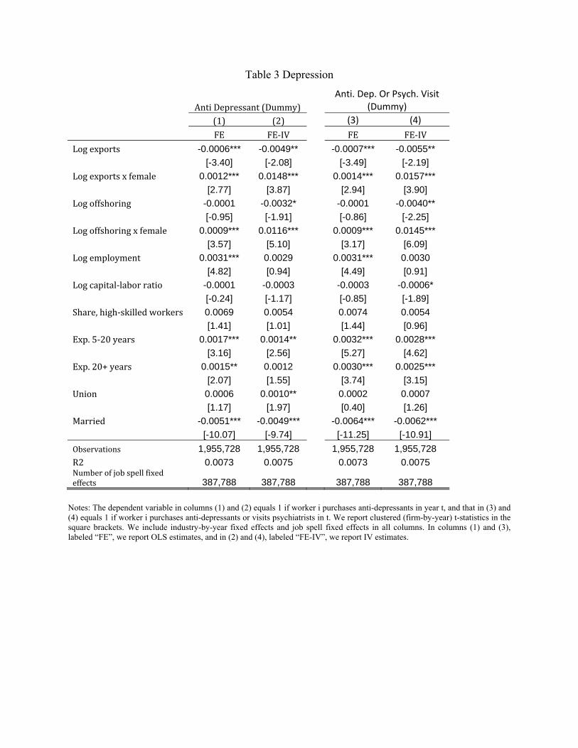
Table 3 Depression

AntiDepressant(Dummy)Anti. Dep. Or Psych. Visit 

(Dummy) 

(1) (2) (3)  (4) 

FE FE‐IV FE FE‐IV

Logexports -0.0006*** -0.0049** -0.0007*** -0.0055**

[-3.40] [-2.08] [-3.49] [-2.19]

Logexportsxfemale 0.0012*** 0.0148*** 0.0014*** 0.0157***

[2.77] [3.87] [2.94] [3.90]

Logoffshoring -0.0001 -0.0032* -0.0001 -0.0040**

[-0.95] [-1.91] [-0.86] [-2.25]

Logoffshoringxfemale 0.0009*** 0.0116*** 0.0009*** 0.0145***

[3.57] [5.10] [3.17] [6.09]

Logemployment 0.0031*** 0.0029 0.0031*** 0.0030

[4.82] [0.94] [4.49] [0.91]

Logcapital‐laborratio -0.0001 -0.0003 -0.0003 -0.0006*

[-0.24] [-1.17] [-0.85] [-1.89]

Share,high‐skilledworkers 0.0069 0.0054 0.0074 0.0054

[1.41] [1.01] [1.44] [0.96]

Exp.5‐20years 0.0017*** 0.0014** 0.0032*** 0.0028***

[3.16] [2.56] [5.27] [4.62]

Exp.20+years 0.0015** 0.0012 0.0030*** 0.0025***

[2.07] [1.55] [3.74] [3.15]

Union 0.0006 0.0010** 0.0002 0.0007

[1.17] [1.97] [0.40] [1.26]

Married -0.0051*** -0.0049*** -0.0064*** -0.0062***

[-10.07] [-9.74] [-11.25] [-10.91]

Observations 1,955,728 1,955,728 1,955,728 1,955,728

R2 0.0073 0.0075 0.0073 0.0075 Numberofjobspellfixedeffects 387,788 387,788    387,788 387,788

Notes: The dependent variable in columns (1) and (2) equals 1 if worker i purchases anti-depressants in year t, and that in (3) and (4) equals 1 if worker i purchases anti-depressants or visits psychiatrists in t. We report clustered (firm-by-year) t-statistics in the square brackets. We include industry-by-year fixed effects and job spell fixed effects in all columns. In columns (1) and (3), labeled “FE”, we report OLS estimates, and in (2) and (4), labeled “FE-IV”, we report IV estimates.

Table 4 Other Sickness Conditions Prescription Drugs for                         

   (1)  (2)  (3)  (4)  (5)  (6) 

Sleep Disorder 

Sleep Disorder 

Heart Disease  

Heart Disease 

Heart Attack or Stroke 

Heart Attack or Stroke 

   FE  FE‐IV  FE  FE‐IV  FE  FE‐IV 

Logexports ‐0.0001  ‐0.0014  0.0002  0.0003  ‐0.0000  ‐0.0012 [‐0.52]  [‐0.68]  [1.57]  [0.26]  [‐0.00]  [‐0.68] 

Logexportsxfemale 0.0005*  0.0005  ‐0.0000  0.0009  ‐0.0002  0.0089*** [1.85]  [0.16]  [‐0.30]  [0.75]  [‐0.84]  [3.51] 

Observations 1,955,728  1,955,728  1,955,728  1,955,728  1,955,728  1,955,728 

R2 0.0017  0.0018  0.0011  0.0012  0.0138  0.0142 Numberofjobspellfixedeffects 387,788  387,788  387,788  387,788  387,788  387,788 

Hospitalization Due to                   

Sleep Disorder 

Sleep Disorder 

Poisoning, Self‐Harm or Assault 

Poisoning, Self‐Harm or Assault 

Heart Attack or Stroke 

Heart Attack or Stroke 

FE  FE‐IV  FE  FE‐IV  FE  FE‐IV 

Logexports 0.0000  0.0003  0.0000  ‐0.0003  0.0000  ‐0.0002 

[0.30]  [0.59]  [0.83]  [‐0.81]  [0.15]  [‐0.34] 

Logexportsxfemale ‐0.0000  0.0003  ‐0.0001  ‐0.0006  ‐0.0000  0.0013* [‐0.11]  [0.81]  [‐1.25]  [‐1.10]  [‐0.48]  [1.90] 

Observations 1,955,728  1,955,728  1,955,728  1,955,728  1,955,728  1,955,728 

R2 0.0002  0.0002  0.0001  0.0001  0.0004  0.0004 

  Numberofjobspellfixedeffects 387,788  387,788     387,788  387,788     387,788  387,788 

Notes: The dependent variables are dummies that equal 1 if worker i has the described sickness conditions in year t. We define the sickness conditions using the ATC codes for the prescription drugs and the ICD-10 codes for the hospitalization diagnoses (see the Appendix for more details). We report clustered (firm-by-year) t-statistics in the square brackets. We include industry-by-year fixed effects and job spell fixed effects in all columns. In the columns labeled “FE” we report OLS estimates, and in those labeled “FE-IV” we report IV estimates.

Table 5 Job Injury

   Dep. Var = Injury Dummy 

FE FE‐IV FE FE‐IVLogexports 0.0004*** 0.0020*

[4.09] [1.71] Logexportsxfemale -0.0001 -0.0017

[-0.71] [-1.42] Exp.2qxmale ‐0.0004*  0.0003 

[‐1.77]  [1.55] 

Exp.2qxfemale ‐0.0002  0.0005** [‐0.85]  [2.05] 

Exp.3qxmale 0.0002  0.0005** [1.27]  [2.52] 

Exp.3qxfemale 0.0003  0.0006*** [1.28]  [2.61] 

Exp.4qxmale 0.0006***  0.0011*** [3.41]  [4.34] 

Exp.4qxfemale 0.0004**  0.0011*** [2.21]  [4.06] 

Logoffshoring -0.0001 0.0022** ‐0.0001  0.0023*** 

[-0.94] [2.56] [‐0.72]  [2.94] 

Logoffshoringxfemale -0.0001 0.0008 ‐0.0001  ‐0.0001 

[-0.75] [0.84] [‐0.89]  [‐0.20] 

Logemployment -0.0004 -0.0036** ‐0.0006**  ‐0.0036*** 

[-1.61] [-2.44] [‐2.17]  [‐4.20] 

Logcapital‐laborratio 0.0004** 0.0003* 0.0003**  0.0003* 

[2.45] [1.88] [2.33]  [1.92] 

Share,high‐skilledworkers -0.0060*** -0.0044* ‐0.0060***  ‐0.0045** 

[-3.20] [-1.94] [‐3.25]  [‐2.35] 

Exp.5‐20years 0.0010*** 0.0010*** 0.0010***  0.0010*** 

[4.35] [4.30] [4.33]  [4.26] 

Exp.20+years 0.0008** 0.0008** 0.0008**  0.0008** 

[2.50] [2.41] [2.49]  [2.41] 

Union 0.0001 0.0001 0.0001  0.0001 

[0.53] [0.43] [0.50]  [0.52] 

Married -0.0002 -0.0002 ‐0.0002  ‐0.0002 

[-0.94] [-1.02] [‐0.93]  [‐1.01] 

Observations 1,955,728 1,955,728 1,955,728  1,955,728 

R2 0.0006 0.0006 387,788  0.0006 

Numberofjobspellfixedeffects 387,788 387,788 0.0006  387,788 

Notes: The dependent variable equals 1 if worker i suffers severe injury in year t that causes permanent damages to her earning and working abilities. The notation “Exp. 2q” means second-quartile export shocks, etc. We report clustered (firm-by-year) t-statistics in the square brackets. We include industry-by-year fixed effects and job spell fixed effects in all columns. In the columns labeled “FE”, we report OLS estimates, and in those labeled “FE-IV” we report IV estimates.

Table 6 Hours and Hours-Based Injury    log(Hours) Inj./ Hours 

FE FE‐IV FE FE‐IV FE‐IV

Logexports -0.0072 -0.0071

[-1.14] [-0.08]

Logexportsxfemale 0.0112* 0.1159*

[1.73] [1.95]

Exp.2qxmale 0.0266***  0.0220***  0.000328 

[3.24]  [3.02]  [0.68] 

Exp.2qxfemale 0.0386***  0.0388***  0.000170 

[5.30]  [5.57]  [0.46] 

Exp.3qxmale 0.0327***  0.0311***  0.000441 

[3.95]  [3.57]  [0.86] 

Exp.3qxfemale 0.0508***  0.0389***  0.000010 

[6.49]  [4.61]  [0.02] 

Exp.4qxmale 0.0009  ‐0.0042  0.001622** 

[0.08]  [‐0.32]  [2.04] 

Exp.4qxfemale 0.0091  0.0142  0.000788 

[1.03]  [1.39]  [1.43] 

Logoffshoring 0.0081*** 0.0270 0.0069**  0.0263  0.000870 

[2.67] [0.74] [2.29]  [0.72]  [0.47] 

Logoffshoringxfemale -0.0031 -0.0757*** ‐0.0023  ‐0.0367**  0.002720** 

[-0.77] [-2.71] [‐0.58]  [‐2.32]  [2.08] 

Logemployment 0.1015*** 0.0799 0.0963***  0.0869**  0.001343***

[4.97] [1.32] [4.46]  [1.97]  [2.62] 

Logcapital‐laborratio 0.0013 0.0019 0.0004  0.0020  0.001420** 

[0.23] [0.32] [0.07]  [0.35]  [1.99] 

Share,high‐skilledworkers 0.1533 0.1899 0.1367  0.1729  0.002045 

[1.35] [1.09] [1.21]  [1.31]  [1.41] 

Exp.5‐20years 0.0986*** 0.0997*** 0.0968***  0.0981***  ‐0.000330 

[24.95] [25.43] [24.89]  [24.78]  [‐0.50] 

Exp.20+years 0.0906*** 0.0920*** 0.0890***  0.0905***  ‐0.005133** 

[23.17] [23.89] [22.99]  [23.08]  [‐2.32] 

Union 0.0020 0.0026 0.0020  0.0017  0.000331 

[0.56] [0.72] [0.58]  [0.49]  [1.15] 

Married 0.0070*** 0.0067*** 0.0065***  0.0067***  0.003271 

[3.14] [3.04] [2.94]  [2.97]  [0.56] 

Observations 1,161,807 1,161,807 1,161,807  1,161,807  1,161,807 

R2 0.0267 0.0265 0.0284  0.0279  0.0006 

Numberoffixedeffects 321,863 321,863 321,863  321,863     321,863 Notes: The dependent variable in the first 4 columns is the log of total (regular plus over time) annual hours, and this variable is only available for a sub-sample of our data. The dependent variable in the last column is the injury dummy divided by the number of total annual hours. The notation “Exp. 2q” means second-quartile export shocks, etc. We report clustered (firm-by-year) t-statistics in the square brackets. We include industry-by-year fixed effects and job spell fixed effects in all columns. In the columns labeled “FE”, we report OLS estimates, and in those labeled “FE-IV” we report IV estimates.

Table 7 Minor Sick-Leave Days

   Dep.Var.=#.MinorSick‐LeaveDays FE FE‐IV FE  FE‐IVLogexports 0.0021 0.0316

[0.63] [0.68] Logexportsxfemale -0.0054 -0.0282

[-1.03] [-0.59] Exp.2qxmale ‐0.0159**  ‐0.0179** 

[‐2.18]  [‐2.11] 

Exp.2qxfemale ‐0.0136  ‐0.0189* [‐1.51]  [‐1.93] 

Exp.3qxmale ‐0.0306***  ‐0.0482*** [‐4.08]  [‐5.47] 

Exp.3qxfemale ‐0.0140  ‐0.0229** [‐1.59]  [‐2.18] 

Exp.4qxmale ‐0.0012  ‐0.0128 [‐0.18]  [‐1.25] 

Exp.4qxfemale ‐0.0063  ‐0.0180 [‐0.81]  [‐1.57] 

Logoffshoring -0.0027 0.0087 ‐0.0022  ‐0.0012 

[-0.94] [0.27] [‐0.76]  [‐0.04] 

Logoffshoringxfemale 0.0105** 0.0725** 0.0099**  0.0578*** 

[2.46] [2.24] [2.31]  [2.67] 

Logemployment -0.0260** -0.0735 ‐0.0223*  ‐0.0192 

[-2.26] [-1.40] [‐1.88]  [‐0.58] 

Logcapital‐laborratio -0.0031 -0.0044 ‐0.0026  ‐0.0046 

[-0.61] [-0.85] [‐0.51]  [‐0.89] 

Share,high‐skilledworkers -0.0505 -0.0271 ‐0.0385  ‐0.0697 

[-0.64] [-0.31] [‐0.49]  [‐0.89] 

Exp.5‐20years -0.0706*** -0.0717*** ‐0.0699***  ‐0.0705*** 

[-5.88] [-5.96] [‐5.83]  [‐5.87] 

Exp.20+years -0.0478*** -0.0493*** ‐0.0470***  ‐0.0482*** 

[-3.03] [-3.12] [‐2.98]  [‐3.05] 

Union 0.0018 0.0027 0.0017  0.0017 

[0.19] [0.30] [0.18]  [0.19] 

Married -0.0266*** -0.0264*** ‐0.0265***  ‐0.0259*** 

[-2.79] [-2.76] [‐2.78]  [‐2.71] 

Observations 1,955,728 1,955,728 1,955,728  1,955,728 

R2 0.0002 0.0002 0.0002  0.0002 

Numberofjobspellfixedeffects 387,788 387,788 387,788  387,788 

Notes: The dependent variable is the number of minor sick-leave days that worker i takes in year t, defined as those sick-leave days during which i neither visits a doctor nor purchases any prescription drug. The notation “Exp. 2q” means second-quartile export shocks, etc. We report clustered (firm-by-year) t-statistics in the square brackets. We include industry-by-year fixed effects and job spell fixed effects in all columns. In the columns labeled “FE”, we report OLS estimates, and in those labeled “FE-IV” we report IV estimates.

Table 8 Major Sick-Leave Days

   Dep.Var.=#.MajorSick‐LeaveDays FE FE‐IV FE  FE‐IV Logexports -0.0175 -2.2137***

[-0.31] [-3.18] Logexportsxfemale 0.5403*** 0.0910

[4.59] [0.10] Exp.2qxmale ‐1.0472***  ‐0.7396*** 

[‐6.79]  [‐6.23] 

Exp.2qxfemale ‐1.3747***  ‐0.5185*** [‐7.08]  [‐2.75] 

Exp.3qxmale ‐0.6644***  ‐0.4284*** [‐5.85]  [‐3.24] 

Exp.3qxfemale ‐0.6795***  ‐0.1020 [‐3.71]  [‐0.51] 

Exp.4qxmale ‐0.1329  0.7188*** [‐1.27]  [4.15] 

Exp.4qxfemale 1.0709***  1.9384*** [6.61]  [8.93] 

Logoffshoring -0.1632*** -1.4407*** ‐0.1508***  ‐0.4205 

[-4.76] [-2.86] [‐4.54]  [‐0.90] 

Logoffshoringxfemale 0.4570*** 6.6662*** 0.4057***  5.9006*** 

[6.90] [12.07] [6.27]  [15.52] 

Logemployment -0.4021** 0.8322 ‐0.5905***  ‐3.1137*** 

[-2.16] [0.90] [‐2.85]  [‐5.54] 

Logcapital‐laborratio -0.0995 -0.1993** ‐0.0980  ‐0.1601* 

[-1.17] [-2.22] [‐1.17]  [‐1.75] 

Share,high‐skilledworkers -2.2972* -4.5427*** ‐1.7705  ‐1.3008 

[-1.79] [-3.03] [‐1.40]  [‐0.99] 

Exp.5‐20years 0.2779** 0.1470 0.2988**  0.1942 

[2.34] [1.24] [2.52]  [1.64] 

Exp.20+years -0.7941*** -0.9620*** ‐0.7684***  ‐0.9032*** 

[-5.16] [-6.26] [‐4.99]  [‐5.88] 

Union 0.5574*** 0.6214*** 0.5543***  0.6940*** 

[5.38] [5.91] [5.34]  [6.63] 

Married -0.9941*** -0.9321*** ‐0.9801***  ‐0.9423*** 

[-9.98] [-9.38] [‐9.85]  [‐9.48] 

Observations 1,955,728 1,955,728 1,955,728  1,955,728 

R2 0.0088 0.0092 0.0091  0.0095 

Numberofjobspellfixedeffects 387,788 387,788 387,788  387,788 

Notes: The dependent variable is the number of major sick-leave days that worker i takes in year t, defined as those sick-leave days during which i purchases prescription drugs, or visits doctors, or both. The notation “Exp. 2q” means second-quartile export shocks, etc. We report clustered (firm-by-year) t-statistics in the square brackets. We include industry-by-year fixed effects and job spell fixed effects in all columns. In the columns labeled “FE”, we report OLS estimates, and in those labeled “FE-IV” we report IV estimates.

Table 9 Heterogeneous Responses and Robustness Exercises

   Anti.Dep.Anti.Dep.OrPsych.

StrokeDrug

StrokeHosp. Injury

Log.Tot.Hours

1.PhysicalStrengthatOccupationLogexports ‐0.0099***  ‐0.0112***  ‐0.0014  ‐0.0006  0.0008  ‐0.0306 

[‐3.91]  [‐4.08]  [‐0.69]  [‐0.76]  [0.65]  [‐0.35] 

Logexportsxfemale 0.0239***  0.0240***  0.0126***  0.0014*  ‐0.0013  0.1333** 

[5.64]  [5.34]  [4.52]  [1.81]  [‐0.92]  [2.24] 

Log exports x Physical  0.0107***  0.0105***  0.0066***  0.0005*  0.0019***  0.0231 

[8.01]  [7.29]  [7.19]  [1.70]  [4.95]  [1.20] 

Observations  1,590,874  1,590,874  1,590,874  1,590,874  1,590,874  1,036,536 

R‐squared  0.0072  0.0071  0.0131  0.0004  0.0008  0.0248 

Number of fixed effects  381,260  381,260  381,260  381,260  381,260  294,704 

2.MentalStrengthatOccupationLogexports ‐0.0073***  ‐0.0090***  ‐0.0001  ‐0.0004  0.0019  ‐0.0261 

[‐3.04]  [‐3.44]  [‐0.07]  [‐0.58]  [1.54]  [‐0.32] 

Logexportsxfemale 0.0197***  0.0201***  0.0097***  0.0013*  ‐0.0021  0.1173** 

[4.76]  [4.61]  [3.45]  [1.71]  [‐1.53]  [2.17] 

Log exports x mental  ‐0.0065***  ‐0.0071***  ‐0.0030***  ‐0.0004  ‐0.0023***  ‐0.0115 

[‐5.32]  [‐5.50]  [‐3.43]  [‐1.40]  [‐4.88]  [‐0.84] 

Observations  1,590,874  1,590,874  1,590,874  1,590,874  1,590,874  1,036,536 

R‐squared  0.0072  0.0071  0.0131  0.0004  0.0008  0.0248 

Number of fixed effects  381,260  381,260  381,260  381,260  381,260  294,704 

3. Age    

Logexports ‐0.0057**  ‐0.0058**  ‐0.0223***  ‐0.0016***  0.0016  0.0168 

[‐2.30]  [‐2.18]  [‐9.16]  [‐2.63]  [1.41]  [0.20] 

Logexportsxfemale 0.0150***  0.0157***  0.0164***  0.0018**  ‐0.0016  0.1093* 

[3.92]  [3.90]  [6.54]  [2.49]  [‐1.26]  [1.85] 

Log exports x Over‐40  0.0024  0.0008  0.0624***  0.0040***  0.0011  ‐0.0539*** 

[1.35]  [0.44]  [16.17]  [7.52]  [1.52]  [‐2.78] 

Observations  1,955,728  1,955,728  1,955,728  1,955,728  1,955,728  1,161,807 

R‐squared  0.0075  0.0075  0.0158  0.0004  0.0006  0.0265 

Number of fixed effects  387,788  387,788  387,788  387,788  387,788  321,863 

4. Continuous Exp.  Logexports ‐0.0039*  ‐0.0048*  ‐0.0016  ‐0.0002  0.0020*  ‐0.0120 

[‐1.70]  [‐1.81]  [‐0.98]  [‐0.33]  [1.80]  [‐0.14] 

Logexportsxfemale 0.0157***  0.0167***  0.0072***  0.0013*  ‐0.0017  0.1116* 

[4.25]  [4.29]  [3.14]  [1.85]  [‐1.35]  [1.90] 

Observations  1,955,728  1,955,728  1,955,728  1,955,728  1,955,728  1,161,807 

R‐squared  0.0082  0.0081  0.0201  0.0005  0.0006  0.0405 

Number of fixed effects  387,788  387,788  387,788  387,788  387,788  321,863 Notes: The dependent variables in the first 5 columns are the dummies that worker i has the described injury or sickness conditions in year t. “Anti. Dep.” is anti-depressant, “Psych.” is psychiatrist visiting, and “Hosp.” is hospitalization. The dependent variable in the last column is the log of total annual hours. We report clustered (firm-by-year) t-statistics in the square brackets. We include industry-by-year fixed effects and job spell fixed effects and report IV estimates in all columns. To save space, we have left out the coefficient estimates of the firm-control and worker-control variables. The former set includes the logs of offshoring, employment, capital-labor ratio, and the share of skilled workers. The latter set includes the dummies for union status, experience and marital status.

Table 9 Heterogeneous Responses and Robustness Exercises, Continued

   Anti.Dep.Anti.Dep.OrPsych.

StrokeDrug

StrokeHosp. Injury

Log.Tot.Hours

5. Log Dom. Output    

Logexports ‐0.0038  ‐0.0046*  ‐0.0010  0.0000  0.0021*  ‐0.0529 

[‐1.58]  [‐1.74]  [‐0.55]  [0.07]  [1.87]  [‐0.60] 

Logexportsxfemale 0.0115***  0.0123***  0.0074***  0.0012*  ‐0.0016  0.0845 

[3.06]  [3.13]  [2.89]  [1.65]  [‐1.27]  [1.33] 

Observations  1,861,512  1,861,512  1,861,512  1,861,512  1,861,512  1,113,834 

R‐squared  0.0074  0.0073  0.0143  0.0004  0.0006  0.0288 

Number of fixed effects  384,154  384,154  384,154  384,154  384,154  317,922 

6. 7+ years job spells    

Logexports ‐0.0030  ‐0.0027  ‐0.0022  ‐0.0021***  0.0022**  ‐0.0667 

[‐1.11]  [‐0.94]  [‐0.96]  [‐2.75]  [1.98]  [‐0.73] 

Logexportsxfemale 0.0171***  0.0200***  0.0136***  0.0034***  ‐0.0020  0.1052* 

[3.36]  [3.72]  [3.76]  [3.23]  [‐1.21]  [1.74] 

Observations  981,941  981,941  981,941  981,941  981,941  604,158 

R‐squared  0.0097  0.0098  0.0183  0.0006  0.0006  0.0306 

Number of fixed effects  105,603  105,603  105,603  105,603  105,603  101,099 

7. 3‐year M.A. of WID    

Logexports ‐0.0034  ‐0.0027  ‐0.0033**  ‐0.0006  0.0029***  0.0078 

[‐1.56]  [‐1.16]  [‐1.99]  [‐0.97]  [3.27]  [0.09] 

Logexportsxfemale 0.0090**  0.0096**  0.0142***  0.0015**  ‐0.0015  0.0993 

[2.34]  [2.37]  [5.67]  [2.16]  [‐1.29]  [1.57] 

Observations  1,955,728  1,955,728  1,955,728  1,955,728  1,955,728  1,161,807 

R‐squared  0.0075  0.0074  0.0142  0.0004  0.0006  0.0265 

Number of fixed effects  387,788  387,788  387,788  387,788  387,788  321,863 

8.LocalLaborMarketTightnessLogexports ‐0.0050**  ‐0.0055**  ‐0.0009  ‐0.0006  0.0015  0.0302 

[‐2.21]  [‐2.26]  [‐0.50]  [‐0.93]  [1.36]  [0.36] 

Logexportsxfemale 0.0147***  0.0156***  0.0088***  0.0015**  ‐0.0017  0.1429** 

[3.87]  [3.89]  [3.47]  [2.09]  [‐1.37]  [2.27] 

Log exports x UI Rate  ‐0.0000  ‐0.0000  ‐0.0000  0.0000  ‐0.000031***  0.0010* 

[‐0.16]  [‐0.40]  [‐0.67]  [0.37]  [‐3.25]  [1.93] 

Observations  1,955,728  1,955,728  1,955,728  1,955,728  1,955,728  1,161,807 

R‐squared  0.0075  0.0075  0.0142  0.0004  0.0006  0.0269 

Number of fixed effects  387,788  387,788  387,788  387,788  387,788  321,863 

Notes: The dependent variables in the first 5 columns are the dummies that worker i has the described injury or sickness conditions in year t. “Anti. Dep.” is anti-depressant, “Psych.” is psychiatrist visiting, and “Hosp.” is hospitalization. The dependent variable in the last column is the log of total annual hours. We report clustered (firm-by-year) t-statistics in the square brackets. We include industry-by-year fixed effects and job spell fixed effects and report IV estimates in all columns. To save space, we have left out the coefficient estimates of the firm-control and worker-control variables. The former set includes the logs of offshoring, employment, capital-labor ratio, and the share of skilled workers. The latter set includes the dummies for union status, experience and marital status.

Table 10 Utility-Loss Calculations

  

Change w.r.t. Exports 

Mean Rate 

% Change w.r.t. Exports 

Share Weight, 

% 

Marginal Dis‐utility (DKK) 

Lower Bound of (5) 

Upper Bound of (5) 

(1)  (2)  (3) = (1)/(2)  (4)  (5)  (6)  (7) 

Men's Incidences of                      

Anti‐Depressants ‐0.0049  0.0242  ‐20.21%  0.41%  36331.87  3125.69  69538.04 

Heart Attacks or Stroke (drugs) 0  0.0204  0.00%  0.05%  5568.35  479.05  10657.65 Heart Attacks or Stroke 

(hospitalization) 0  0.0005  0.00%  1.89%  7762600.38  667829.59  14857371.16 

Injury 0.002  0.0043  46.76%  3.10%  1556842.20  133937.76  2979746.63 

Women's Incidences of                      

Anti‐Depressants 0.0099  0.0395  25.09%  0.41%  12994.37  1117.93  24870.82 

Heart Attacks or Stroke (drugs) 0.0077  0.0100  77.01%  0.05%  6629.06  570.31  12687.80 Heart Attacks or Stroke 

(hospitalization) 0.0011  0.0007  150.11%  1.89%  3230268.85  277905.47  6182632.23 

Injury 0.002  0.0031  63.50%  3.10%  1231138.81  105916.95  2356360.66 

Notes: The numbers in column (1) are our estimates in Tables 3-5. They are 0 for men’s rates of heart attacks or strokes because the coefficient estimates are not statistically significant.

The numbers in column (3) are the values for ln

gp

in equation (15). The numbers in column (4) are calculated using Table A5 and they are the values for βg in (15). The values in

column (5) are calculated using columns (2), (4) and equation (20).