\

l )

\~

NOAA Technical Memorandum NWS WR-190

GREAT SALT LAKE EFFECT SNOWFALL: SOME NOTES AND AN EXAMPLE

David M. Carpenter

National Weather Service Forecast Office Salt Lake City, Utah October 1985

UNITED STATES I National Oceanic and I National Weather DEPARTMENT OF COMMERCE Atmospheric Administration Service Malcolm Baldrige, Secretary John V. Byrne. Administrator Richard E. Hallgren. Director

This pub1ication has been reviewed

and is approved for pub1ication by

Scientific Services Division,

Western Region.

i i

~scfhi~ Scientific Services Division Western Region Headquarters Sa1t Lake City, Utah

TABLE OF CONTENTS

PAGE

I. Introduction 1

II. Elements of a Great Salt Lake Effect Snowstorm 2

III. An Example 11

IV. Summary 14

v. Acknowledgments 15

VI. References 16

i i i

Great Salt Lake Effect Snowfall: Some Notes and an Example David M. Carpenter

National Weather Service Forecast Office Salt Lake City, Utah

I. Introduction

A lake effect snowfall along the Wasatch Front is typically a post cold frontal event in which the duration of snowfall downwind of the lee shore is extended in cold, northwest flow. Where one would normally expect snowfall to end with the passage of the upper level trough, lake effect snows usually continue for several hours after that event.

This paper is based on data taken from lake effect cases that occurred in the northwest flow following the passage of an upper level trough. Occasionally it appears that a lake effect may have occurred in southwest flow, which enhances snowfall close to

or the

produces northeast

shoreline. These cases are relatively infrequent and are not included in this study. The necessity of a rapid infusion of cold air, usually in the form of a cold pocket, and the fact that this air would have to come from a southerly direction makes a conventional lake effect hard to come by. What probably occurs in most cases when snowfall is heavier along the northeast shoreline is a warm advection pattern associated with a cut-off low over Nevada as described by Williams (1962). Terrain produced upslope and differential friction from the lake surface to the shoreline would enhance snowfall in that vicinity, but a contribution of instability and moisture from the Great Salt Lake to the air mass is probably not a factor in most of these cases. Even after limiting the study to storms that occur in north­west flow, the effect of the Great Salt Lake on snowfall is not one that can be easily measured.

Following are some ideas result­ing from the study of the various elements which should contribute to Great Salt Lake effect snowfalls. Twenty one lake effect cases dating from March 1971 to October 1984 were used. The last case October 18, 1984, is used as an example of a lake effect storm. This storm resulted in the heaviest 24 hour snowfall on record at the Salt Lake Interna­tional airport. All of the cases produced four or more inches of snow at some point in the valley and seven of them produced over a foot. This set of data is not intended to represent a complete listing of all Great Salt Lake effect cases which occurred during this time period. Instead, it is more likely to be a representation of the most dramatic or most noticeable cases.

The percentage of annual snowfall in the Salt Lake Valley which may be attributable to lake effect is not known. However, the average number of lake effect cases per year has been estimated to be between 6 and 8 (Alder,l977). The average number of days per year in which 0.1 inch of snow or more is measured at the Salt Lake Interna­tional Airport is 34 (Figgins,l984). Other studies indicate that lake effect from the Great Salt Lake probably occurs a rather small percentage of the time (Dunn, 1983). Considering these facts and the restrictive nature of the required temperatures and wind flows necessary to produce a lake effect, it is felt by most of the forecasting staff at the Salt Lake International Airport

that the total contribution df lake effect snowfall to the annual snowfall of the Salt Lake Valley1 and nearby areas is probably rather small. Nevertheless, the lake effect can produce dramatic results, and . is the object of much interest and specu­lation among those who watch the weather along the Wasatch Front.

II. Elements of a Great Salt Lake effect Snowstorm

A. Topographical Influences

The Lake is literally surrounded by mountain ranges which at one time formed islands and the shoreline (Fig. 1). The most prominent of these north-south mountain ranges is the Wasatch Range. The Great Salt Lake is oriented approximately along the 320 degree radial from the Salt Lake International Airport. The longest fetch, or over water trajectory, is approximately 75 miles long along that 320 degree radial. This fetch is realized in northwest flow for the Salt Lake Valley and in northerly flow for the Tooele Valley. Both valleys slope upward away from the Lake shore and form a rough half bowl shape.

In addition to upslope, the topography makes two other modifi­cations to the surface wind that are worthy of note. The first of these is illustrated in Figure 2. An exaggeration of a ·s.imple balance of forces is used to explain frictional convergence · along the lee shore of

1 The term Salt Lake Va'lley will be used to refer to the S~l t Lake City metropolitan area including all municipalities near Salt Lake City and located west of the Wasatch Mountains and east of the Oquirrh Mountains, south of the Great Salt Lake and north of the Transverse Mountains. The Transverse Mountains are shown in Figure 1 as the point of the Mountain just north of Alpine.

2

Brigham 0

"" 423~ <

1

OgderJr-L?: 4300"' 0 ( :::>

LL o ~~:0::

Figure 1 -Map of the Great' Salt Lake and surrounding topographical · fea­tures.

the Lake (Hess,l959). In reality the dynamics and kinematics of this process are much more complicated. At all four points,. the pressure gradient force (PG) is the same, but the frictional drag force (F) varies with the roughness of the surface. Over the relatively smooth lake surface the frictional force is less than that over land. Therefore, the wind velocity (V) is greater over the lake than over land. This difference in speed is enough to cause an area of low level convergence along the lee shoreline (Lavoie,l972). The second modification to the low level flow is the channeling that occurs as air is pushed against the sides of the mountain ranges.

Figure 3 shows the resulting streamlines of a hypothetical case of

N I

i -w--,-~

i ' s

Figure 2 - A simple balance of forces illustration of the effect of differ­ential friction on the surface wind flow in the vicinity of the Great Salt Lake.

northwest, low level flow. Note that the channeling effect and the backing of the wind as it moves onshore, combine to produce low level convergence in the upper portions of the Tooele Valley and along the east bench area of the Salt Lake Valley.

During some lake effect storms, the s~rface wind at the Salt Lake International Airport has been known to shift to the southwest and then to the southeast, while the wind at nearby surrounding stations remains northwesterly. This is possibly a reflection of something called a local front or boundary layer front by Garner (Garner,l983). This is something similar to a miniature New England Coastal Front (Bosart, Vaudo, and Helsdon, 1972).

3

N '

w--~-E I s

. >' \/

Figure 3 - An idealized illustration of the surface stre811Jline analysis of northwest flow when the effects of differential friction and channelling by the Wasatch Front are taken into account.

In a Great Salt Lake local front, cold air at the surface becomes dammed up against the mountains in the upper portion of the valley and forms a small cold dome (Figure 4). Then, the low level flow coming off the Great Salt Lake rides up and over this cold dome, producing vertical motion. The colder air in the valley is maintained as being colder than the air coming off the Lake by convective down drafts and precipi­tation. Eventually with the help of a frictional disturbance along the lee shoreline, the flow in the valley becomes detached from the larger scale flow and can switch to a southerly direction. Without meso­scale data to confirm the above

4

~---~

Figure 4 - Illustration of Great Salt Lake local front and cold air damming.

scenario, it is mostly conjecture, but not unreasonable.

B. Temperature of the Lake

The temperature of the Great Salt Lake is important to Lake Effect snowfall for two reasons: one, it indicates the amount of energy available in. the surface of the Lake that may be transferred to the lowest layers of the atmosphere, to produce convection; and two, it determines the maximum allowable saturation vapor pressure of the air mass over the lake, for a transfer of moisture to occur between the Lake and the air mass (Ellenton and Danard, 1979). Since the Great Salt Lake brine has a

reduced vapor pressure compared to fresh water, the second consideration

cannot be overlooked. This will be dealt with in another section.

For the purpose of this study, it would be best to have a record of Great Salt Lake temperature measure·· ments for several locations at the same time of the day over many years. For the purpose of real time forecasting, it would be best to have the same temperature data available in real time. However, neither of these situations is the case and we will have to settle for data taken at one point (the southern shore near the Salt Air Resort), twice a month by the United States Geological Survey. These data were then compared to the previous seven days actual mean air temperature at the Salt Lake International Airport (Figure 5) and to the normal mean air temperature of the airport (Figure 6). Two least squares curves were fitted to the data to predict the temperature of the Great Salt Lake. Figures 5 and 6 show the resulting least squares curves (solid lines with dots) and the distribution of data points about the curves (detached lines with dots). The correlation coefficient for the curve in figure 5 is 0.88 with a standard error of 4.78 degrees F. For figure 6, the correlation coefficient is 0.91 with a standard error of 4.21 degrees F.

For the 21 cases used in this study, the average Great Salt Lake temperature computed from the 7 day mean curve was 44.6. The average Lake temperature computed from the normal curve was 45.2. There is an obvious difference in the predicted Great Salt Lake temperature between the two curves. For example, using a temperature of 37 degrees F for the normal mean, produces a Lake temp­erature estimate of 42.6, while a 7 day mean temperature of 37 degrees F results in a Lake temperature estimate of 38.9 degrees F. Even though the difference is small in

L A K E

T E M p

E R A T u R E

c 20-

15-

10·

5- . ) 0"

-5-

·15 -10 -5 tO t5 20

PREVIOUS 7 DAY ACTUAL MEAN TEMPERATURE c

Figure 5 Comparison of Great Salt Lake temperature verses the average of the previous · 7 days actual mean air temperature for the Salt Lake City International Airport.

this example. it is easy to see that a period of abnormally warm or cold temperatures could cause a large difference in the two estimates.

Considering the size of the standard error for these two curves, as long as real time data on the temperature of the Lake are not available, an average of the two predictions will normally produce an acceptable prediction of the Great Salt Lake temperature. Averaging the two predictions will allow for an abnormally warm spell to be taken into account.

C. Instability Criteria

One of the necessary (but not sufficient) conditions for a signifi­cant Great Salt Lake effect snowfall is an unstable layer of air of sufficient depth to produce snow. This instability is achieved when the Lake is warm enough and/or the

5

c

20-

L A rf K 15 E •'\t T ... t--._tf· !V E 1\r /v . M i . r p

E 5

(\y/V R A T u o- I . R E ,./ -5- .

-t5 -to -5 to 15

NORMAL MEAN TEMPERATURE

Figure 6 - Comparison of Great Salt Lake Temperature verses the normal mean temperature at the Salt Lake Airport for the date.

air mass aloft is cold enough to create a lapse rate which is moist adiabatic or greater. A convenient way to measure this is to use the temperature difference between the Lake and 700 mb (Rothrock,' 1969). For comparison, using a surface pressure of 870 mb ( a typical surface pressure ) and a Lake temp­erature of 5 degrees C, a moist adiabatic lapse rate results in a Lake to 700 mb temperature difference of around 10 degrees C and a dry adiabatic lapse rate in a difference of around 17 degrees C.

The optimum Lake to 700 mb temp­erature difference appeared to be between 17 and 23 degrees C. Differ­ences much greater than this (25 degrees or more) seemed to cause a decrease in convective activity rather than an increase. Temper­atures of minus 18 degrees C at 700 mb were not uncommon in these cases. This is probably due to several factors related to the cold nature of

20

c

the air mass involved, but the most important of these is probably the fact that air which is that cold is generally very stable, and the lake effect convection is not strong enough to compensate for that stability.

D. Vapor Pressure Differential

The Great Salt Lake brine has a reduced vapor pressure compared to that of fresh water. A study was conducted to determine vapor.pressure as a function of brine concentration and temperature (Dickson,Yepson, and Hales, 1965). The results are illustrated in figure 7. The first two curves, labeled Es(29.2%) and Es(24.7%), show the resulting vapor pressure vs. temperature curves for the Lake for two values of brine concentration. The curve labeled Es is the same distribution for distilled water.

! '. I I I 35 i

i )0

I I

~I 25

~I 20

~! 15 T' u: :! 1o

00 i 5

. 0

-5.

I !

I I

·.\.1 I .

i: I

I

Figure 7 - Saturation vapor pressure taken over Great Salt Lake brine for varying degrees of salinity and over distilled water verses· the teJJJp­erature. Taken from Dickson, Yepson Hales, 1965).

6

A necessary requirement for a transfer of moisture from the Lake to the air mass, is that the vapor pressure over the Great Salt Lake brine must be greater.than the vapor pressure of the overlying air mass. For example using the point on the 24;7% curve (Es(24.7)) corresponding to a Lake temperature of 10 degrees C, we follow a constant vapor pressure line down to the distilled water curve (Es) and then read the temperature on the scale on the left. The dewpoint temperature of the overlying air mass must be less than this temperature for a transfer of moisture to occur between the Lake and the air mass. In this case the dewpoint temperature of the air mass must be less than about 6.5 degrees C. Given the condition that the salinity of the Great Salt Lake is probably less than even 24.7% , a rough rule of thumb could be that a Lake to dewpoint temperature differ­ence of 5 degrees C or greater would satisfy this condition.

The change in the precipitable water · value in the downstream air mass as a result of Lake Effect is probably only a few hundredths of an inch. However since we are dealing with precipitable water values in the .10 to .40 inch range, and consider­ing that the vertical motions produced by the terrain effects and convection can be considerable, the effect of this increase is worth mentioning (Harley, 1965).

If one were to assign all the elements of Great Salt Lake lake effect snow, a degree of importance in contributing to the rate of snowfall, it is felt that the vertical motion produced by low level convergence and upslope and the addition of sensible heat to the lower levels of the atmosphere, should receive a higher ranking than the addition of moisture by the lake.

\ ! ' I

E. Inversion Height

A limiting factor to lake effect snowfall and one which is strongly correlated to the end of the snowfall is the height of the subsidence inversion following the 700 mb trough (Rothrock, 1969). The height of this· inversion serves to limit the vertical extent of the convective cloud tops. Rawinsonde traces from the 21 cases in this s'tudy . indicate that an inversion height between 650 and 700 mb is probably the m1n1mum for production of any precipitation. Once the inversion drops below 700 mb most storms are more or less over.

F. Weak Upper Disturbances

One ingredient that is apparently necessary for a significant lake effect is the presence of a weak upper level disturbance. This disturbance is often not shown in the operational vorticity analyses due to the large spacing between upper air stations. Most of the time the disturbance will show up as a temperature trough at 700 mb. The surface pressure trace may also reflect its presence in a slight hesitation, or a flat spot on an otherwise r1s1ng trace. ~ven though a few of the cases showed this, no common pattern was observed.

G. Location of Snowfall vs. Wind Direction

The data confirms the assumption that the direction of wind flow determines the location of the heaviest concentration of snow. The areas which received a discernable concentration of heavy snow during a lake effect were for the most part limited to four locations. These are shown in Figure 8. Area l appears to receive the most lake effect snow­fall. Area 2 is not well covered with climatological stations, and there­fore will not be represented very

7

Figure 8 - Areas which receive 1 ake effect snow.

well in the following discussion of that.data. However notes taken at the Salt Lake City forecast office show a strong tendency for lake effect in this area. The third area includes the east foothill area of Salt Lake City and the valley floor from about 2100 south northward. This is possibly just an extension of the first area northward, but there does appear to be a separate response to wind direction. The fourth area is in the Tooele Valley near the town of Tooele. The fifth area is from Davis county northward, but as was mentioned before, no cases for this situation are included in this study.

Figure 9 is included to allow a comparison to the normal water equivalent precipitation for the months October through April. The rema1n1ng maps (figures 10 through 17) are cumulative water equivalent, storm total precipitations for groupings of lake effect storms. The intention is to show a pattern of snowfall rather than to imply a

s:sr -o-PatkVallqo

Figure 9 October through April normals for water equivalent precip­itation in the vicinity of the Great Salt Lake.

quantitative average of some kind.The 700 mb wind direction was used for two reasons; one, it is conven­ient to obtain since it is routinely observed and, it is not as subject to frequent fluctuations due to terrain or local drainage effects.

Data are only presented for situations in which three or more cases would apply. In figures 11 through 17, each case was categorized using the average 700 mb wind direc­tion, during the lake effect. Many cases are . included in two maps because c; their average 700 mb wind direction was an even multiple of ten and thus fell on the line between two categories. Figure 10 shows the cumulative precipitation for all Lake Effect cases. Note that the area of maximum snowfall extends . approx­imately from Bountiful southward to Sandy, and has been drawn to include Little Cottonwood Canyon to Alta (see Figure 18 for these locations). This

8 -· .o-PArilVa!lq

/. g"7 ;:.5'2 ...J.P "'~

Figure 10 Total water equivalent precipitation for all of the 21 Lake Effect snowfall cases in the stud.v.

comprises areas 1 and 3 mentioned above. A complete set of data for Alta was not available in the monthly Utah Climatological Data Publication, which was used in this study. However, it is felt by the author that Alta would easily fall within the 15 inch isopleth.

Figures 11 and 12 show the precipitation data for cases with an average 700 mb wind direction from 330 to 350 degrees inclusive. The greatest maximum of heavy snow is located in the Tooele Valley, or area 4 as described above. Area 2, or the western portion of the Salt Lake Valley also receives heavy snowfall in many of these cases. A dramatic switch in the location of the greatest maximum eye occurs when the 700 mb wind direction becomes more westerly. This is shown in Figure 13 with the average 700 mb wind direction from 320 to 330 degrees (inclusive). The heavy snowfall greatest maximum in this case is

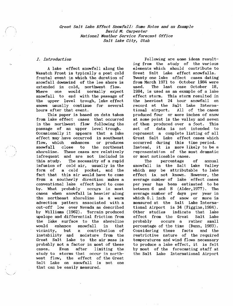
located in the southern portion of the Salt Lake Valley, or area 1. Average 700 mb wind directions from 290 to 320 degrees produce essentially the same results (figures 13 through 16). As the wind direction becomes even more westerly as in figure 17, a. new maximum center appears to develop along the east bench area of the city or area three. A study of the mean precipitation for a number of cases vs. 700 mb wind direction for the Salt Lake Airport, Tooele, Alta, and others was conducted by Elliot, Thompson, and Griffith (1985). The results of that study agree with the patterns shown in this section.

Figure 11 Total water equivalent precipitation for all Lake Effect cases in which the average 700mb wind direction was from 340 to 350 degrees (inclusive).

9

.3/ •E..rJ.

~~~;an Fk. PM~<?:{ Par:~cnrSE

?7 S.tnjaQu~. 0,55' • '0- <> .¢- Tho"l•2'1'1

[lbHU

Figure 12 Total water equivalent precipitation for all Lake cases in whi cb the average 700 mb wind dir­ection was from 330 to 340 degrees ( inclusive).

Figure 13 Total water equivalent precipitation for all Lake cases in which the average 700 mb ¥dnd dir­ection was from 320 to 330 degrees (inclusive).

10

.13 "((-0up;~r

.I/ ,.,.,..-o-

Figure 14 precipitation which the

Total water equivalent for ~11 .Lake cases in

average 700 mb wind dir-ection was (inclusive).

from 310 to 320 degrees

Figure 15 Total water equivalent precipitation for all .Lake cases in which the average 700 mb wind dir­ection was from 300 to 310 degrees (inclusive).

Figure 16 p1·ecipitation fo1· all which the average 700 ecti on was from 290

Total water equivalent

( inclusive).

Lake mb

cases in wind dir-

300 degrees to

Figure 17 Total water equivalent precipitation for all Lake cases in which the average 700 mb wi11d dir­ection was from 280 to 290 degrees ( i11clusive).

/ III. An Example

On October 17-18, 1984 a record 18.4 inches of snow fell at the Salt Lake City International Airport. This surpassed the previous heaviest 24 hour accumulation of 18.1 inches, which fell in December 1972. All but one inch of this record amount fell between 6:30p.m. MDT on the 17th and 11:30 a.m. on the 18th. The heavy snow fell in a relatively small area in the lee of the Great Salt Lake, including the area from southern Davis County to southern Salt Lake County, generally east of the meridian of the airport (Figure 18). Little or no snow fell on the west side of the valley. It resulted in approximately one million dollars damage to the Salt Lake City area, due mostly to downed power lines and broken trees which

11

had not yet shed their leaves. This storm contained many of the elements of a classic lake effect snowstorm.

The temperature of · the Great Salt Lake was estimated to be around 10 degrees C. This was later con­firmed by a call to the United States Geological Survey, who had measured the · temperature a few days before the event.

Figure 19 shows the 700 mb height and temperature analysis for 12Z on the 18th. Note the strong cold advection which occurred during the event. Temperatures at 700 mb would have maintained a Lake to 700 mb difference greater than 17 degrees C throughout the time in question. The average 700mb wind direction-was

Figure 19 - 700 mb analysis for 12Z October 18, 1984. Note tile slmzp temperature trough.

290 degrees. Note the temperature trough indicating the weak disturb­ance embedded in the northwest flow. Figures 20, 21, and 22 show the 500 mb height and ·vorticity analyses for the period. Note that during the time from OOZ on the 18th to OOZ on the 19th, 500 mb vorticity advection over Northern Utah was either negative or neutral.

The precipitable water values for the western U.S. at 12Z on the 18th are shown in figure 23. 'Note first of all the difference between Salt Lake's value and those up­stream. Second note the air mass alone would not be capable of produc­ing the 1.76 inches of water which fell.

Figures 24 and 25 show the surface analyses for 06Z and 18Z on the 18th. Surface winds at the airport remained out of the northwest during the storm,

12

Figure 20 NMC · 500 inb height and vorticity analysis for OOZ Thursday October 18, 1984.

Figure 21 .NMC 500 mb height and vorticity B11alysis for 12Z Thursday October 18, 1984.

Figure 22 - NMC 500 mb vorticity analysis for October 19, 1984.

height and ooz Friday

\

' ' ' --.:k ' ,• .......... -~-- .. __ ',

' ,r-- ..... __ _

' ' ·- ("-'

' ' '~ ' ' /

-,-'

- --J. ------.28--:- .. ----0 GGW 72 ~

--:- ... ----------- ........ -~ :--·

"'.._ .57 I :

I •- • 0 J. .69.------1 ' ' --.110 I ,---~ ELP

i --.--~-- 144

13

Figure 23 Precipitable water (top number) and percent of normal (bottom) for the Western States3 12Z Thursday October 18; 1984.

Figure 24 Surface analysis for the Western States for 06Z Thursday October 18, 1984.

Figure 25 - Surface analysis for the Western States for 18Z Thursday October 18, 1984.

then shifted to southwesterly at l8Z. The wind shift was possibly an indication of the development of a local front. The Salt Lake City dewpoint temperature remained at a steady 31 degrees F while surrounding stations are in some cases 10 degrees F lower. Upstream dewpoints in this case were in the neighborhood of -5 degrees C. This produces a Lake to air mass dewpoint temperature diff­erence of about 15 degrees C. As discussed earlier, a difference of only 5 degrees is necessary for a transfer of moisture from the Lake to the atmosphere.

Another factor was a jet streak which passed just south of Salt Lake City (Figures 26 and 27). The left front quadrant of the jet streak probably passed over the area between 06Z and 12Z on the 18th, which was the time of heaviest snowfall. Due to missing data for several stations

' I

' :r(/ lfD......:.i;, ,,

' ' P• ,

' ...... :. .....

' .

' ' ' ' '

.... ,, ~- .. --~-',~-~:~--~--~--~--~J

! .v 0 .... ;-·A·~----1

:\\\\. ',~··! ' :~ '-- ..........

'\f------0

'

I I

' ' I

' ' .......... 1. ........ ,

po

' ' , ..

fO

Figure 26 a11alysis .for 1.984.

250 mb f'li11ds a11d isotach OOZ Thursday October 18,

' .. ,~~t

' J

.-, ' ' ' ' I

I I I

I

' ' ' ' ' ' -·,;:-...... ..... .. ', .. 30- .... \

' ' ' ,... : //d : ,, '

t , ' ... '.. Jlf. ,' . PJJ I

"-- -~ ~ -~ ' ! ': '~ ...... ~ ...... ~- ·~, ""-=-.. ?J"'-' I 0 I \\ •

Fi!.ru.re 27 250 mb w.i11ds tmd isotach analysis for 12Z Thursday October 18, 1984.

14

011 the 122 map, the exact pattern of isotach contours is unknown. This quadra11t of the jet streak }Vou1d provide dynamic support to the coJJVect..i 011 i11 the fonn of upM.trd vertical motion.

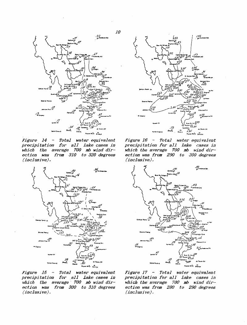
The GOES 6 p_ictures in figures 28 through 30 sbow the dissipat.ion s t:age of the cloud cover over the Lake during the last few hours of the storm. Early i11 the course of' events, the Lake is nearly covered with clouds. Tl1e cloud cotter then (Ussipates .from north to south un U 1 only a narrow bcwd re.mE:l.ins along the southeastern shore at around lBZ.

IV. Swnmar_v

The cond.i ti ons ently necessary

wlli ch are appar­for Great Se:J 1 t

S110wfall could be · Lake 1 ake effect

Figure 28 - OOES 6 picture f'or 12302, Thursda_v October 18, 1.984.

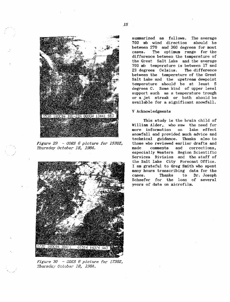
Figure 29 - GOES 6 picture for 1530Z, Thursday October 18, 1984.

Figure 30 - GOES 6 picture for 1730Z, Thursday October 18, 1984.

15

summarized as follows. The average 700 mb wind direction should be between 270 and 360 degrees for most cases. The optimum range for the difference between the temperature of the Great Salt Lake and the average 700 mb temperature is between 17 and 23 degrees Celsius. The difference between the temperature of the Great Salt Lake and the upstream dewpoint temperature should be at least 5 degrees C. Some kind of upper level support such as a temperature trough or a jet streak or both should be available for a significant snowfall.

V Acknowledgments

This study is the brain child of William Alder, who saw the need for more information on lake effect snowfall and provided much advice and technical guidance. Thanks also to those who reviewed earlier drafts and made comments and corrections, especially Western Region Scientific Services Division and the staff of the Salt Lake City Forecast Office. I am grateful to Greg Smith who spent many hours transcribing data for the cases. Thanks to Dr. Joseph Schaefer for the loan of several years of data on microfilm.

16

REFERENCES Alder.,~. William J. 1 1977: Unpublished notes on Great Salt Lake.Effect Snowfall.

National Weatner Service Forecast Office, 337 North 2370 West, Salt lake City, Utah 84116

Bosart, Lance F., Vaudo, Cosmo J. and Helsdon, John H.i 1972: Coastal Frontogenes1s. Journal of Applied Meteorology 11 236-1258

Dickson, Don R., Yepson, John H. and Hales, J. Vern, 1965: Saturated Vapor Pressures over Great Salt Lake Brine. Journal of Geophysical Research 70 500-503

Dunn, Lawrence B.,l983: Quantitative and Spacial Distribution of Winter Precipitation Along Utah's Wasatch Front. NOAA Technical Memorandum NWS WR-181

Ellenton, Gloria E. and Danard, Maurice B.i 1979: Inclusion of Sensible Heating in Convective Parameterization App ied to Lake Effect Snow. Monthly Weather Review 107 551-565

Elliot, Robert D., Thompson, John R., and Griffith, Don A., 1985: Estimated Impacts of West Desert Pumping on Local Weather. NAWC Report SLWM.85-l. North American Weather Consultants 8-1 - 8-9

Figgins, Wilbur E. 1984: Climate of Salt Lake City Utah 2nd Revision. NOAA Technical Memorandum NWS WR-152

Garner, Stephen, 1983: A Linear Analysis of Relevance to Local Frontogenesis. Tnesis proposal. Massachusetts Institute of Technology, Cambridge, Massachusetts 02139

Harley, w.s,, 1965: An Operational Method for Quantitative Precipitation Forecas~ing. Journal of Applied Meteorology 4 no. 3 305-319

Hess, Seymour L., 1959: Introduction to Theoretical Meteorology. Holt, Rinehart, and Winston. 179-180

Lavoie, Ronald L., 1972: A Mesoscale Numerical Model of Lake-Effect Storms. Monthly Weather Review 29 1029-1040

Rothrock1 H.J., 1969: An Aid to Forecasting Significant Lake Snows. ESSA • Tecnnical Memorandum WBTM CR-30

Williams, Philip Jr., 1962: Forecasting the Formation of Cutoff Lows Over the Wes~ern Plateau. U.S. Weather Bureau Manuscript, Salt Lake City, Utah