Western Region

SALT LAKE CITY, UTAH

April 1972

NOAA TM NWS WR74

NOAA Technical Memorandum NWS WR74 U.S. DEPARTMENT OF COMMERCE National Oceanic and Atmospheric Administration National Weather Service

Thunderstorms and Hail Days Probabilities in Nevada

CLARENCE M. SAKAMOTO

NOAA TECI:INICAL MEMORANDA National Weather Service, Western Region Subseries-

The Nationa·l Weather Service (NWSl Western Region <WRl Subseries provides an ·informal medium for the documentation and quick dissemination of results not appropriate, or not yet ready, for ·formal pub! !cation. The series is used to report on work In progress, to describe technical ·procedures and practices, or to relate progress to a llmi'ted audience. These Technical Memoranda will report on investigations devoted primarily to regional and local problems of interest mainly to personnel, and hence will not be widely distributed.

Papers I to .23 are in_ the former series, ESSA Techn.lcal Memorand~, Western Region Technical Memoranda CWRTMl; papers 24"to 59 are· in the former perles, ESSA Technical Memoranda; Weather Bureau Technical Memoranda (WBTMl. Beginning wlth.60, the papers are part of the serie.s, NOAA Technical. Memor<!nda NWS.

Papers I to 23, except for 5 (revised edition) and 10, are avai fable from the National Weather Service Western Region, Scientific Services Division, P. 0. Box 11188, Federal Sui I ding; 125 South State Street; salt Lake City, Utah 841 I I. Papers.S (revised edition), 10, and alI others beginning with 24 are aval fable from the National Technical Information Service, U.S. Department of Commerce, Sills Bldg., 5285 Port·Royai.Road., Springfield, Va. 22151. Price: $3.00 paper copy; $0.95 microfiche. Order by accession number shown In parentheses at end of ·each entry.

WRTM I WRTM 2 WRTM 3

WRTM 4 WRTM 5

WRTM 6 WRTM7 WRTM 8 1'/RTM 9 1'/RTM 10 WRTM II WRTM 12

WRTM 13

WRTM 14

WRTM 15

WRTM 16· 1'/RTM 17

WRTM 18 WRTM 19

WRTM 20

WRTM 21

WRTM 22 WRTM 23

WBTM 24

WBTM 25

WBTM 26 WBTM 27 WBTM 28 WBTM 29 WBTM 30

WBTM 31

WBTM 32

WBTM 33 WBTM 34 WBTM 35

WBTM 36

WBTM 37 WBTM 38

WBTM 39 WBTM 40 WBTM 41 WBTM 42

WBTM 43 WBTM 44

WBTM 45/1

ESSA Technical Memoranda

Some Notes on Probabi I ity Forecasting. Edward D. Diemer, September 1965. (Out of print.) Cl imatologlcal Precipitation Probabll ities. Compiled by Lucianna Miller, December 1965. Western Region Pre- and Post-FP-3 Program, December I, 1965 to February 20, 1966. Edward D. Diemer, March 1966. . Use of Meteoro I og i ca I Sate.! I i te Data. March 1966. Station Descriptions of Local· Effects on Synoptic Weather Patterns. Philip Wi II lams, Jr.·, April 1966 (revised November 1967, October 1969), <PB-178000) Improvement of Forecast Wording a~d Format. C.· L. Glenn, May 1966. Final Report on Precipitation Probability Test Programs. Edward D. Diemer, May 1966. Interpreting the RAREP. Herbert P. Benner, May 1966 (revised January 1967). (Out of print.) A Col faction of Papers Related to_ the 1966 NMC Primitive-Equation Model. June 1966. Sonic Boom. Loren Crow (6th Weather Wing, USAF, Pamphlet), June 1966. (Out of print.) (AD-479366) Some Electrical Processes in the Atmosphere. J, Latham, June 1966. · A Comparison of Fog Incidence at Missoula, Montana, with Surrounding Locations. Richard A. Dightman, August l9(i6. (Out of print.) · A Col feet ion of Technical Attachments on the 1966-NMC Primitive-Equation Model. Leonard W. Snel !man, Aug us+ I 966. <Out of prInt. l · Appl !cation of Net Radiometer Measurements to Short-Range Fog and Stratus Forecasting at Los Angeles. Frederick Thomas, September 1966. The Use of the Mean as an Estimate of "Normal" Precipitation In an Arid Region. Paul C. Kangleser, November 1966. Some Notes on Ace! imatlzation in Man. A Digitalized Summary of Radar Echoes L. B. Overaas, December 1966.

Ed I ted by Leonard w; Snellman, November 1966. Within 100 Miles of Sacramento, Cal lfornla. J .• A. Youngberg and

Limitations of Selected Meteorologicai Data. December 1966. A Grid Method for Estimating Precipitation Amounts by Using the WSR-57 Radar. R. Granger, December 1966. (Out of print.) ·

Transmitting Radar: E:c.ho ·Locat_ions to Local Fire Control Agencies for. Ljghtni.ng F'.re Detecflon.· Robert R. Pei·erson, March 1967. (Out of print.) An Objective Aid for Forecasting· the End of East Winds in the Columbia Gorge, July through October. D. John Coparan is, April 1967. · · Derivation of Radar Horizons In Mountainous Terrain. Roger G. Pappas April 1967. "K" Chart App I icat Ions to Thunderstorm -Forecasts. Over the Western United States. Richard E. Hamb; dge May 1967. '

ESSA Technical Memoranda, Weather Bureau. Tec~nical Memoranda <WBTMl

Historical. and Cl imatologlcal Study of Grinnel I Glacier, Montana. Richard A. Dightman, July 1967. CPB-178071)

Verification of Operational Probabi I ity of Precipitation Forecasts, Apr! 1 1966-March 1967. w. w. D·ickey, October 1967. (PB-176240) A Study of Winds in the Lake Mead Recreation Area. R. P. Augul is, January 1968. (PB-177830) Objective Minimum Temperature Forecasting for Helena, Montana. D. E. Olsen, F-ebruary 1968. (PB-177827) Weather Extremes. R. J. Schmid! i, April 1968 (revised July 1968). CPB-178928) . Smal 1-Scale Analysis and Prediction. Phi I ip Wil I iams,·Jr., May 1968. (PB-178425) Numerical Weather Prediction and Synoptic Meteorology. Capt. Thomas D. Murphy U.S.A.F. May 1968. CAD-673365) ' ' Precipitation Detection Probabi I !ties by Salt Lake ARTC Radars. Robert K. Belesky, July 1968. CPB-179084)

Probabi I ity Forecasting--A Problem Analysis with Reference to the Portland Fire Weather District. Harold s. Ayer, July 1968. CPB-179289) · Objective Forecasting. Phi lip Williams, Jr., August 1968. <AD-680425) Th7 WSR-57 Radar Program at Missoula, Montana. R. Granger, Octob~r 1968. (PB-180292) Jo1nt ESSA/FAA ARTC Radar Weather Survei I lance Program. Herbert P. Benner and DeVon B. Smith, December 1968 (revised June 1970). CAD-681857) Temperature Trends in Sacramento--Another Heat Is I and. Anthony D. LentIni , February i969. (Out of print. l (PB-183055)

Disposal of Logging Re7idues Without_ Damage to Air Qual lty. Owen P. Cramer, March 1969. (PB-i83057) Climate of Phoenix, Arizona. R. J, Schmid II, P. C. Kangieser, and R. S. Ingram. Apri 1 1969. (Out of print.). (PB-184295) Upper-Air Lows Over Northwestern United States.· A. L. Jacobson, April 1969. (PB-184296) The Man-Machine Mix in Appl led Weather Forecasting in the 1970s. L. W. Snellman August 1969 (PB-185068) High Resolution Radiosonde Observations. w. s. Jqhnson, August 1969. (PB-185673l ' Analysis of the Southern Cal ifornla Santa Ana of January 15-17, 1966. Barry B. Aronovitch Augu·st 1969 (PB-185670) ' ' Forecasting Max i·mum Temper_atures at He I ena ,_ Montana. David E. 01 sen, October 1969. (PB-185762) Estimated Return Periods for Short-Duration Precipitation in Arizona. Paul c. Kangieser, October 1969. (PB-187763) Precipitation Probabii !ties in the Western Region Associated with Winter-500-mb Map Types. Richard A. Augul is, December i969. (P8-i88248l · ·

·:;.J.

U. S. DEPARTMENT OF COMMERCE NATIONAL OCEANIC AND ATMOSPHERIC ADMINISTRATION

NATIONAL WEATHER SERVICE

NOAA Technical Memorandum NWSTM WR-74

THUNDERSTORMS AND HAIL DAYS PROBABILITIES IN NEVADA

WESTERN REGION

Clarence M. Sakamoto . Climatologist for Nevada

National Weather Service Reno, Nevada

TECHNICAL MEMORANDUM NO. 74

SALT LAKE CITY, UTAH APRll 1972

List

I.

II.

Ill.

IV.

v. VI.

VII.

TABLE OF CONTENTS

of Tables

Introduction

Procedure

Data

Computer Program

Results

Acknowledgment

References

i i

i i i-iv

2-4

4

4-6

6-8

8

8

LIST OF TABLES

Table I. Summary of Model Selection for Thunderstorm and Hal I Days in Nevada · 9

Table 2A. Computed and Observed Cumulative Probabi I ities of Monthly Number of Thunderstorm Days at Elko, Nevada, January - June 10

Table 2B. Computed and Observed Cumulative Probabi I ities of Monthly Number of Thunderstorm Days at Elko, Nevada, July - December I I

Table 3A. Computed and Observed Cumulative Probabi I ities of Monthly Number of Thunderstorm Days at Ely, Nevada, January - June 12

Table 3B. Computed and Observed Cumulative Probabi I ities of Month I y Number of Thunderstorm Days at E I y, Nevada, July -December 13

Table 4A Computed and Observed Cumulative Proba~i I ities of Monthly Number of Thunderstorm Days at Las Vegas, Nevada, January - June 14

Table 4B. Computed and Observed Cumulative Probabi I ities of Monthly Number of Thunderstorm Days at Las Vegas, Nevada, July - December 15

Table 5A. Computed and Observed Cumulative Probabi I ities of Monthly Number of Thunderstorm Days at Reno, Nevada, Jahuary -June 16

Table 5B. Computed and Observed Cumulative Probabi I itles of Monthly Number of Thunderstorm Days at Reno, Nevada, July - December 17

Table 6A. Computed and Observed Cumulative Probabi I ities of Monthly Number of Thunderstorm Days at Winnemucca, Nevada, January- June 18

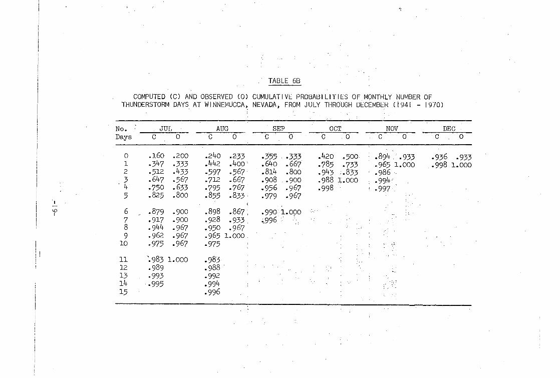
Table 6B. Computed and Observed Cumulative Probabilities of Monthly Number of Thunderstorm Days at Winnemucca, Nevada,/ July -December 19

Table 7. Mean and Variance of Annual Thunderstorm and Annual Hai I Days at Five Locations in Nevada 20

Table 8. Calculated and Observed Cumulative Probaui I ities of Annual Thunderstorm Days at Five Locations in Nevada

iii

--·--------------

21

LIST OF TABLES (Continued)

Table 9. Calculated and Observed Cumulative Probabi I ities of Annual Hai.l Day~ at Five Locations in Nevada 22

Table 10. Sample Program Output Showing the Maximum Likelihood Parameter Estimate and Probabi I ities for Selected Number of Thunderstorm Days at Ely, Nevada 23

Table I I. Sample Program Output Showing Probabi! ities of Selected Number of Annual Hai I Days at Winnemucca, Nevada 24

Table 12. Comparison of Parameter K Estimates by Method of Maximum Likelihood, Method of Moments and "By Eye" for Thunderstorm Probabi I ities in Nevada 25

iv

I •

THUNDERSTORM AND HAIL DAYS PROBABILITIES IN NEVADA

ABSTRACT

A computer program was developed to p'rovide probabi I ities for selected number of thunderstorm days in a month and in a year. In addition, probabi I ities for selected.number of hai I days in a year were deter­mined. Two distribution models were tested in the analysis: (a) Poisson and (b) negative binomial. The program determines which of these two models is appropriate. Furthermore, if the negative bino­mial model is selected, tests are conducted to 'determine whether estimation of the parameters is to be made by the method of moments or by the method of maximum I ike! ihood. A procedure for estimating efficient estimates of the parameters uti I izing reiterative process and the curvilinear model is described. Estimates by this procedure compare favorably with those obtained "by eye".

The program was applied to five locations in Nevada. Results show that for Nevada, the Poisson distribution fits the monthly thunder­storm days for the months November through Apri I, while the negative binomial fits this variable better from May through October. The negative binomial model also fits the annual thunderstorm days in Nevada. Annual hall days distribution favored the Poisson dJstrlbu­tion where the frequency was smal I. The negative binomial fitted the annual hail days distributi.on at Ely and Elko. Cumulative probabi I ities are presented for these variables at the five sites, including Elko, Ely, Las Vegas, Reno, and Winnemucca.

I. INTRODUCTION

Frequency of thunderstorms or hal I in an area can be an important concern in planning for an instal latlon of equipment or manpower. Thunderstorms also imply the posslbi I ity of flash floods, and, con­sequently, necessary precautions must be considered in the develop­ment of a watershed for its varied uses.

Climatological probabilities provide quantitative information on the chance of occurrence of these meteorological phenomena and can be useful in a decision where cost-benefit analysis is vital. The purpose of this study is to analyze the frequency of occurrence of thunderstorm and ha i I days in Nevada and to derive probab i I iti es for these events.

A thunderstorm day is defined as the occurrence-day of at least one thunderstorm cloud (cumulonimbus) accompanied by I ightning and thunder. It may or may not be accompanied by strong gusts of wind, rain, or hai I. A hai I day is a day when preclpitation in the form of ice is produced by convective clouds. During the winter, smaller-sized frozen droplets fa I I, usually smaller in size than hai I. These are called "small hai I" and, for the purpose of this study, "small hai I" and hai I have not been differentiated.

II • PROCEDURE

Them (6) has indicated that the Poisson or the negative binomial dis­tribution can be potentially applied to rare events, such as tornado frequency, tropical cyclone frequency, hal I frequency, etc. The Poisson distribution has the mean equal to the vari·ance. If the variance increases above the mean, the distribution tends to fit the negative b i nomi a I . Genera I fzed guide I i nes as to which of the two models is appropriate are available but, until the proper tests are conducted, one cannot objectively determine which model is appropriate. A test of hypothesis, using x2 distribution with n-1 degrees of free­dom,is used to determine whether the Poisson or the negative binomial distribution is desirable. It is given by:

X2 = n-1

----LX ( I )

LX

where: variable x is the number of event days and n is the sample size.

The Poisson probability function is gtven by:

x e-l.l l.l XT f (x) =

where: f(X) is the probabi I ity of having, for example, exactly x hal I days for the period in question. J.l is the population mean.

(2)

Expressed in natural logarithms, the Poisson density function is:

1n P = x1n x - 1n x ! - x where: Pis the probabi I ity of exactly x hail days and x

is the sample mean.

(3)

The negative· binomial probabi I ity function can be given by (I):

(k+x-1)! X p

f(x) = ----- [ ] k + X (1 + p) x! (k-1)!

where: k and pare the parameters of the distribution.

(4)

These parameters can be initially estimated by the method of moments:

-2-

- 2 X

k (5)

= s2 - X

and s2 - X

p = X

where: x and s 2 are the sample mean and variance, respectively.

Expressed in natural logarithms, the density function for the negative b i nom i a I i s :

1

1n P = k 1nC---1 + p

+ 1n K + x 1n(--­P + 1

( 6)

where: P is the probabi I lty of x event days for the period in question.

K is defined as:

(k+x-1)! K = (7)

X ! ( k-1) !

The moments method of estimating the parameters p and k is not always efficient. Fisher (3) has provided equation 8, a method of testing whether the efficiency of the moments method is less than 90% by:

1 C=(1+-) (k+2)

p (8)

If C < 20, the method of maxi mum I ike I I hood estimates shou I d be used. If C>20, the method of moments suffices.

The maximum I ike! ihood procedure involves writing the I ike! !hood function,

n

L =II f(x.,p,k) I

1=1

(9)

and max1m1zing the logarithm of L, by taking the partial derivative of the logarithm of L with respect to p and k. When set to zero,

-3-

and solving, the two parameter estimates are determined. Taking the partial derivative of equation (4) with respect to p, and setting to zero>

L = 1

a log L

ap

L:x = ---

p

n k + L:x ----= 0 ( I 0)

1 + p

Substituting x for L:x/n, the mean of the sample is found to be the product of the parameters. Thus x = k p is the first equation.

Taking the partial derivative with respect to k, setting to zero, and using Haldane's (4) equation, which does not involve gamma func­tions, we obtain:

L 2

a log L X

= --- = kn I og Cl + -) 1 - [ ( g + g + · · · gR) + ak k 1 2

k k (g + g3 + ..• + gR) + (g3 + g4 + ..• + gR) +

k+1 2 k+2

k (gR) ... +--...;...;..-]=0 ( I I )

k + R - 1

where·g 1 , g2 , •••. gR are the observed frequ~ncies for the numb~r of thunderstorm or hal I days, x = 1, 2, ..• , R 1s the largest x. x = sample mean; n = number of years; k = paramster estimate. Thom (7) suggests solving this equation by trisl and error or by plotting a few values of L2 against k. The vaJue of kat L2 = 0 is the final estimate of the maximum I ikel ihood estimator of the parameter k. The maximum I ikel ihood estimator of p is solved by substituting k in x = kp which was previously obtained.

I I I • DATA

Two sources of records were utilized to summarize information needed for the analysis. These were the Local Climatological Data (8) and the Climatological Records Book for each location.

IV. COMPUTER PROGRAM

A FORTRAN IV program was developed for the analysis of thunderstorm and hail days that facilitates the solution to the estimation of

-4-

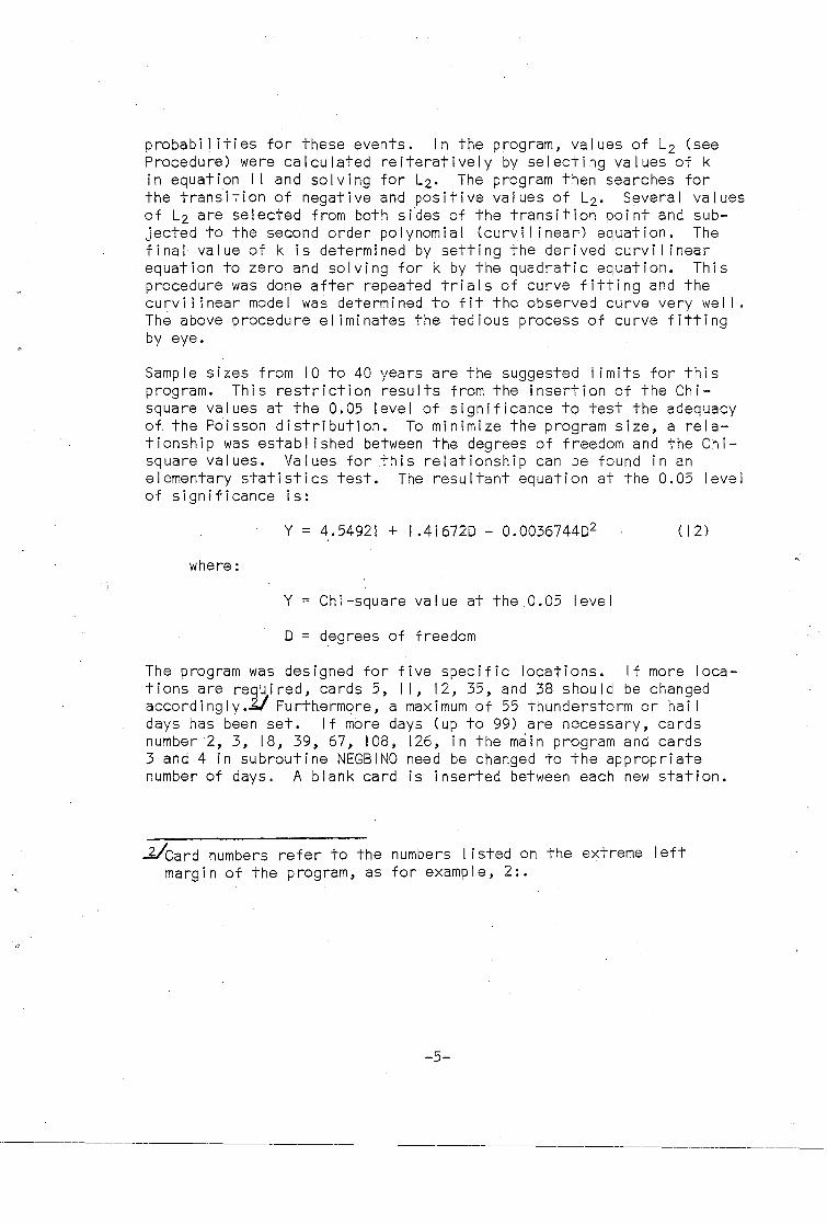
probabilities for these events. In the program, values of L2 (see Procedure) were calculated reiteratively by selecting values of k in equation I I and solving for L2 • The program then searches for the traniition of negative and positive values of L2 • Several values of L2 are selected from both sides of the transition point and sub­jected to the second order polynomial (curvi I inear) equation. The final value of k is determined by setting the derived curvi I inear equation to zero and solving fork by the quadratic equation. This procedure was done after repeated trials of curve fitting and the curvi I inear model was determined to fit the observed curve very wei I. The above procedure eliminates the tedious process of curve fitting by eye.

Sample sizes from 10 to 40 years are the suggested I imits for this program. This restriction results from the insertion of the Chi­square values at the 0.05 level of significance to test the adequacy of. the Poisson distribution. To minimize the program size, a rela­tionship was established between the degrees of freedom and the Chi­square values. Values for .this relationship can be found in an elementary statistics test. The resultant equation at the 0.05 level of significance is:

Y = 4.54921 + I .416720- 0.003674402 ( I 2)

where:

Y =Chi-square value at the 0.05 level

D = degrees of freedom

The program was designed for five specific locations. If more loca­tionsare reguired, cards 5, II, 12, 35, and 38 should be changed accordingly.~ Furthermore, a maximum of 55 thunderstorm or hai I days has been set. If more days (up to 99) are necessary, cards number 2, 3, 18, 39, 67, 108, 126, in the main program and cards 3 and 4 in subroutine NEGBINO need be changed to the appropriate number of days. A blank card is inserted between each new station.

~Card numbers refer to the numbers I isted on the extreme left margin of the program, as for example, 2:.

-5-

Card format is as follows. Blanks are read as zeros.

Co I umns Remarks

1-2 Blank

3-6 Station number

7 Blank

8-1 I Year (for monitor purpose; not necessary in program)

13-16 January (01) and number of thunderstorms (00 to 55)

17 Blank

18-21 February (02) and number of thunderstorms (00 to 55)

22 Blank

23-26 March (03) and number of thunderstorms (00 to 55), etc.

72 Blank

73-74 Annual thunderstorm days (00 to 55)

75 Blank

76-77 Annual hai I days. (00 to 55)

78-80 Blank

V. RESULTS

Probability Models

Table I shows the summary of model selection for the five locations in Nevada. The results indicate that for the monthly distribution, model selection for estimating probabilities of selected number of thunder­storm days depends on the season, and hence, the climate of a parti­cular region. The data suggest that for the period from November through April, the Poisson model is preferred in Nevada, while the negative binomial distribution is appropriate for the period May through October.

-6-

There werG I I cases where the selected model did not coincide with the majority model. However, seven of these cases involved maximum differences of less than .023 between the Poisson and negative bino­mial distribution. The maximum difference between these two models in the other four cases was .108 for zero number of thunderstorm days. In view of the few cases with these differehces, the results of the computer selection were retained in the probabi I ity tables shown in Tables 2A through 68, which also show the observed cumula­tive distribution. The observed and computed probabilities were compared and tested with the Kolmogorov-Smirnov test (5) and alI results were within tolerance at the .10 level of significance.

For annual thunderstorm days, the negative binomial model was selec­ted at alI stations. For annual hai I days, however, only Ely and Elko were associated with the negative binomial; whereas, Reno, Winnemucca, and Las Vegas were fitted with the Poisson distribution. As shown in Table 7, the means at Ely and Elko are larger than the other three sites. Furthermore, the variance is considerably larger than the mean at Ely and Elko. The selection of either of two models for probabi I ities of annual number of hai I days in Nevada suggests that climatic difference is a factor in the selection of the distribution model. Therefore, each climatic region should be analyzed separately to determine the proper selection of the model that fits the data. Calculated cumulative probabi I ities from the model as wei I as observed cumulative frequencies for annual thunder­storm and annual hai I days are shown in Tables 8 and 9, respectively. The Ko I mogorov-Sm i rnov test showed that the se I ected mode Is fitted the observed data at the . 10 level of significance.

I I lustration of reading these probability tables follows: The compu­ted probabi I ities for "O" number of thunderstorm or hai I days are the chance. of none occurring at each of the sites. For example, in Table 9, the probabi I ity of no.hai I at Las Vegas is .875. The probability of exactly x number of hai I days, for example, x = 5 days at Ely is .717 minus .596 or .121; the probabi I ity of less than 5 days is .717; the probabi I ity of greater than 5 hai I days at Ely is 1.000 minus .717 or .283. Probabi I ities for other s~lected number of days and sites are determined similarly.

Computer Outputs

Sample outputs from the computer program are shown in Tables 10 and I I. Table 10 i I lustrates an example of the output for the negative bino­mial distribution, uti I izing the maximum I ikel ihood procedure for estimating the parameters k and p. Table II is an example of the out­put for annual hai I days probabi I ities at Winnemucca.

Comparison of the computer program procedure used for estimating the parameter k, when L2 (Equation I I) is zero and that for estimating k by graphical (eye) procedure is shown in Table 12. Estimate of the parameter by the method of moments is also included. Excel lent agree­ment is indicated by the results between the computer and "by eye".

-7-

It is cone I uded that the procedure uti I i zed in this study is both a rei iable and a rapid method for calculating the parameters of the negative binomial distribution by the maximum I ikel ihood method.

VI. ACKNOWLEDGMENT

This study started as a joint term paper with my wife, Winifred, in her Computer Programming course at the University of Nevada. Through this project we both learned th.e rudiments of computer pro­gramming with many of its frustrating moments. Dr. Young Koh, Col lege of Agriculture Statistician, was helpful and aided our ·efforts when the program seemed imposs i b I e to debug. To these two, the author expresses sincere gratitude.

VI I. REFERENCES

I. BLISS, C. 1., and R. A. Fisher. "Fitting the Negative Binomial Distribution to Biological Data," Biometrias, pp. 176-196, June 1953.

2. FISHER, R. A. "Note on the Efficient.Fitting of the Negative Binomial," Biometrias., pp. 197-200, June 1953.

3. FISHER, R. A. "The Negative Binomial Distribution," Annals of Eugenias., Vol. I I, pp. 182-1~7, 1941.

4. HALDANE, J. B. S. "The Fitting of Binomial Distributions," Annals of Eugenias., Vo I • II , ·pp, 179-181 , I 941 .

5 · · MASSEY_, F. J., Jr. "The Ko lmC?gorov-Sm i rnov Test for Goodness of Fit," Ameriaan Statistiaal Assoaiation Journal, Vo I. 46·; pp. 68-78, 1951.

6. THOM, H. C. S. "Some Methods of Climatological Analysis," World MeteoroZogiaal Organization Teahniaal Note No. 81, pp. 30-34, 1966.

7. THOM, H. C. S. "The Frequency of Ha i I Occurrence," Arahiv fur Meteo­rologie., Geophysik und BiokZimatologie, Series B, Band 8, 2, Heft, pp. 185-194, 1957.

8. U. S. DEPARTMENT OF COMMERCE, National Oceanic and Atmospheric Admin i st rat ion, Env i ronmenta I -Data Service. LoaaZ CZimato Zogi­aal Data for Reno, Ely., Elko., Las Vegas, Winnemuaaa.

9. WILLIAMSON, E., and M. H. BRETHERTON. Tables of the Negative Binomial wobabiZity Distribution., pp. 7-15;, John Wiley and Sons, 1963.

-8-

TABLE I

SUMMARY OF MODEL SELECTION FOR THUNDERSTORM AND HAIL DAYS IN NEVADA

Location Period

Ely Reno El ko Winnemucca Las Vegas

Jan P* None p p p

Feb N p p p p

Mar p p p p p

Apr p p p p N

May N N N N p

J un N N p N p

Jul N N p N N

Aug N N N N N

Sep N p N N N

Oct N .N N p N Nov p N p N p

Dec p N p p p

Ann N N N N N

Annual Ha i I N p N p p

*P = Poisson; N = Negative Binomial

-9-

----------------- ------ ------------------ - ------------- --------- ----- --- --- ---- --- ---- - ---------- ------ ----- --------- ---- - -------- -

.~

?;._

I

0 I

No. Days

0 1 2 3 4 5

6 7 8 9

10

11 12 13 14 15

TABLE 2A

COMPUTED.(C) AND OBSERVED (0) CUMULATIVE PROBABILlTIES OF MONTHLY NUMBER OF THUNDERSTORM DAYS AT ELKO, NEVADA, FROM JANUARY THROUGH JUNE ( 1941 - 1970)

JAN c o·

.875 .867 -992 1.000

1.000.

FEB c 0

• 717 .~·733 ·955 -933 -995 1.000

MAR c 0

.693 -700

.947 -933 -994 1.000 ·999

APR c 0

-393 .500 .760 .zoo -931 .867 .985 1.000 -997

:MAY c 0

.114 .033

.273 .300

.432 .433· ··572 .633 .685 4767 -773 .833

'

JUN c 0

.020 .-067

.10:2 .• ,167

.258 .:333

.460 ~400

.655 .• 500

.806 -733

.839 .867 .903 .967

.887 .867 -956 .967 -922 .900 .982 1.000 .946 .goo .993 .963 .900 -998

-9'15 .900 .983 1.000 -989 ~993 -995

No. Days

0 1 2 3 4 5

I 6 --I 7

8 9

10

11 12 13 14 15

16

0

TABLE 2B '

COMPUTED (C) AND OBSERVED (0) CUMULATIVE PROBABILITIES OF MONTHLY NUMBER OF THUNDERSTORM DAYS AT ELKO, NEVADA, FROM JULY THROUGH DECEMBER (1941 - 1970)

JUL AUG c 0 c 0

.oo6 • 033 .o63 .100 .

.038 .067 .180 -~67

.119 .167 .324 .300

.256 .400 .468 .467

.429 .4oo -597 •.500

.6o4' -533 • 704 ' • 667

-752 .633 .789 .767 .860 .800 .851 .867 -928 -933 .897 .900 .966 .967 -930 -933 .985: 1.000 -953 1.000

-994 .969 -998 .980

.987 -991. -995

. -997

SEP c. 0

-317 -33.3 -587 -533 .766 .?67 .872 .867 -932 .967 .964 .967

.982 .967 -991 1.000 -995

OCT c 0

.636 .633

.858 .833

.944 .967 -977 .967 -991 1.000 -996

NOV G 0

.819 .800· .

.983 1.000. -999

DEC c 0

.875 .867 -992 1.000

1.000

'\

I -N I

No.

TABLE 3A

COMPUTED (C) AND OBSERVED (0) CUMULATIVE PROBABILITIES OF MONTHLY NUMBER OF THUNDERSTORM DAYS AT ELY, NEVADA, FROM JANUARY THROUGH JUNE (1941 - 1970)

JAN FEB MAR APR MAY Days c 0 c 0 c 0 c 0 c 0

0 .905 -900 .903 .900 .648 .667 .231 .300 .661 .033 1 -995 1.000 .963 -933 -929 -900 .569 -533 .185 ~166 2 .984 1.000 -990 1.000 .817 .833 .340 .433 3 -992 .·999 -938 .900 .495 .500 4 -996 .983 .966 .632 .600 5 -996 . -996 1.000 .742 .633

6 .825 .867 7 .884 -933 8 .925 -933 9 -953 -933

10 -970 .967

11 .982 .• 967 12 .989 1.000 13 -993 14 -996 15

16 17 18 19 20

JUN c 0

.038 .067

.118 .100

.228 .233 -350 .266 .471 .400 .581 .600

.676 .667 -754 .800 .817 .900 .865 -933 .902 -933

-930 --933 -950 -933 -965 .967 -976 .967 .983 .• 967

.988 .967 -992 .967 -995 .967 -996 1.000

TABLE 3B

COMPUTED (C) AND OBSERVED (0) CUMULATIVE PROBABILITIES OF MONTHLY NUMBER OF THUNDERSTORM DAYS AT ELY, NEVADA, FROM JULY THROUGH DECEMBER (1941 - 1970)

No. JUL AUG SEP OCT NOV DEC Days c 0 c 0. c o· c 0 c 0 c 0

0 .021 .033 .005 .000 .192 .133 .466 .467 -716 .700 -766 .8oo· 1 .068 .100 .024 .QOO .442 .500. .706 .700 -955 .967 -970 -933 2. .135 .167 .062 .100 .654 -700 .837 .833 -995 1.000 -997 1:.000 3 .217 .233 .120 .100 .801 -733 .909 .900 4 .305 .267 .196 .266 .891 .900 .949 -933 5 -395 .367 - .285 .266 .943 .967 -971 .967

6 .480 .Lr66 -379 ·-333 -971 .967 .984 1.000 7 .560 .500 .474 .400 .986 .967 -991 8 . 632. -533 .563 -566 . 993 1.000 -995 9 I .695 .633 .644 .633 -997 -997 .

10 -750 -733 -716 .667

11 -?96 .766 ·776 .800 I ·12 .835 .833 .827 .867 -

lN 13 .868 ~866 .867 -934 I

14 .894 .866 -900 -934 15 .916 .966 -925 .967

16 -934 .966 .· -945 .967 17 .• 948 .966 .960 .• 967 18 -959 1.000 -971 .967 19 .968 -979 .967 20 -975 .985 .967

21 .981 -989 .967 22 .985 -992 .967 23 .• 988 -995 ·.967 24 -991 -996 1.000 25 -993

26 -995 27 -996

I -.J'>. I

TABLE 4A

COMPUTED {C) AND OBSERVED {0) CUMULATIVE PROBABILITIES OF MONTHLY NUMBER OF THUNDERSTORM DAYS AT LAS VEGAS, NEVADA, FROM JANUARY THROUGH JUNE (1940-1971)

No. JAN FEB MAR APR MAY JUN Days G 0 c 0 G 0 G 0 G 0 c

0 .967 .967 -792 .833 .875 .833 .642 .633 .380 .400 .407 1 LOOO 1.000 -977 .967 -992 1.000 .858 .867 -7~8 -700 -773 2 -942 -933 .926 .967 -937

0 ..,

.400 -767 -933 -~ 998 l. 000 . 1. 000

3 -976 .967 .983 .967 .987 1.000 4 -989 1.000 -997 1.000 -998 5 -996

I -. \.Jl

I

No.

TABLE 4B

COMPUTED (C) AND OBSERVED (0) CUMULATIVE PROBABILITIES OF MONTHLY NUMBER OF THUNDERSTORM DAYS AT LAS VEGAS • NEVADA •. FROM JULY THROUGH DECEMBER ( 1941-1 971 )

JUL AUG SEP OCT NOV DEC Days c 0 c 0 c 0 c 0 c 0 c

0 .032 .067 .110 .166 .3B1 ~400 -5B1 .567 .B47 .B67 -967

·0

.967 1 .11B .167 .• 262 .166 .661 •. 600 -750 .Boo .988 .900 1.000 1.000 2 .251 .:300 .416 .400 .B25 .Boo .B3B .B67 -999 1.000 3 .406 .367 -553 .633 -913 .967 .B91 .900 4 -558 -500 .666 .633 -958 .967 .925 1.000 5 .68B .633 -755 .700 .9BO .967 ~94B

6 -790 .'700 .B23 .Boo -991 1.000 .963 .B64 .B67 .B74 .B33 -996 -974 7

B .915 -900 .911 -933 .9Bl 9 .949 1.000 -937 .• 967 -98.6

10 -970 -956 .967 -9.90

11. ·983 ,. . -970 ~967 ;;993 12 -990 -979 1.000 -995 13 -995 .9B6 . -996 14 -997 -990 15 -993

16 -996

No. Days

0 1 2. 3 4

I 5 -0\ I 6

7 B 9

10

11 12 13 14 15

TABLE 5A

COMPUTED (C) AND 9BSERVED (0) CUMULATIVE PROBABILITIES OF MONTHLY NUMBER OF THUNDERSTORM DAYS AT REN0 1 NEVADA 1 FROM JANUARY THROUGH JUNE (1941 - 1970)

JAN FEB MAR APR MAY JUN c 0 c 0 c 0 c 0 c 0 c

1.000 1.000 .967 .967 -936 -933 .670 .633 .230 .200 .191 1..000 1.000 -99B 1.000 ~938 .967 .479 .467 -396

-992 1.000 .673 .667 -570 -999 .Bo4 .Boo .702

.B87 .900 -79B -936 .900 .B65

.965 1.000 .911

.9B1 .942 -990 .962 -995 -975 -997 .9B4

0

.167

.433

.567 -700 .Boo .867

.900 -933 .967 .967 .967

-990 1.000 -994· -996

No. Days

-0 1 2 3 4 5

6 7

I 8 --..J

9 I

10

11 12 13 14 15

16 17 18 19 20

TABLE 58 COMPUTED (C) AND OBSERVED (0) CUMULATIVE PROBABILITIES.OF MONTHLY NUMBER OF THUNDERSTORM DAYS AT RENO, NEVADA, FROM JULY THROUGH DECEMBER ( 1941 - 1970) 1

JUL AUG c 0 c 0

.085 .167 .256 .233

.228 .200 .449 .500

.389 -333 -594 .633

.540 .466 -700 .667

.666 .567 -780 ..• 767 -765 -733. .838 .800

.838 .900 .881 .867

.891 -933 -912 .900

.928 .967 . . ~936 .900 -953 ..• 967 -970 1.000

.981

.988 -992 -995

-953 .967 ..• 965 .967'

-975 .967 -981 1.000 • 986 -990 -993

-995 -996

SEP OCT NOV DEC c 0 .·c o c 0 c 0

.380 .433 .807 .833 .945 .967 .945 .967 -748 -733 .925 .967 -991 .967 . ~991. .967 -9~6 • 867 .966 .967 •998 1.000 . -998 1.000 .983. -967 .984 -967 . -997 1.000 -992 .967 .

-996 1".000

•' .

I -(X)

I

No.

TABLE 6A

COMPUTED (C) AND OBSERVED (0) CUMULATIVE PROBABILITIES OF MONTHLY NUMBER OF THUNDERSTORM DAYS AT WINNEMUCCA, NEVADA, FROM JANUARY THROUGH JUNE (1941 - 1970)

JAN FEB MAR APR MAY . JUN -Days c. o· c 0 c 0 c 0 c 0 c 0

0 -967 -967 .B75 -900 .B19 .Boo .435 .367 .219 .233 . .146 .167 1 1. ooo 1. odb · -992 -967 .9B3 l.OOO -797 -933 .421 .367 -32B .. 333 2 -1.000 1.000 -999 .94B .967 .581 .633 .497 ' .467 3 I -990 1.000 .701 .767 .635 .633 4 ,998 .7B9 .Boo .742 .667 5 .... .852 .B33 .821 .Boo

6 .B97 . . B67 .B?B .B67 7 .929 -933 -917 .967 8 -951 .967 .944 .967 9 .966 . -967 .963 .967

10 -977 1.000 -976 i.ooo

11 .984 -9B4 12 .9B9 -990 13 -993 -993 14 -995 -996 15 -997

I -1.0 I

'1

TABLE 6B

COMPUTED (C) AND OBSERVED (0) CUMULATIVE PROBABILITIES OF MONTHLY NUMBER OF THUNDERSTORM DAYS AT WINNEMUCCA, NEVADA, FROM JULY THROUGH DECEMBER (1941 - 1970)

No. JUL AUG Days c 0 c 0

0 .160 .200 .240 .2-33 1 .347 -333 .442 .400' 2 -512 .433 -597 .567 3 .647 .567 -712 .667

'4 -750 .633 -795 -767 5 .825 • Boo .B55 .833.

6 .B79 .900 .B9B .B67 i

7 • 917 .900 .928 -933 8 -944 .967 -950 .967 9 .962 .967 .965 1.000

10 -975 .967 -975

11 ~9B3 1.000 .9B3 12 . 989 .98B . 13 -993 -992 14 -995 -994 15 -996

SEP c 0

-355 -333 .640 .667 .B14 .Boo .90B . -900 -956 .967 -979 .967

.990 l.OQO ...

•.996 .

OCT c 0

.420 .500 -7B5 -733 .943 .B33 .9BB 1.000 -998

NOV c 0

.B94. -933

.965 1.000

.9B6 -994' -997 .

DEC c 0

-936 -933 -99B 1.000

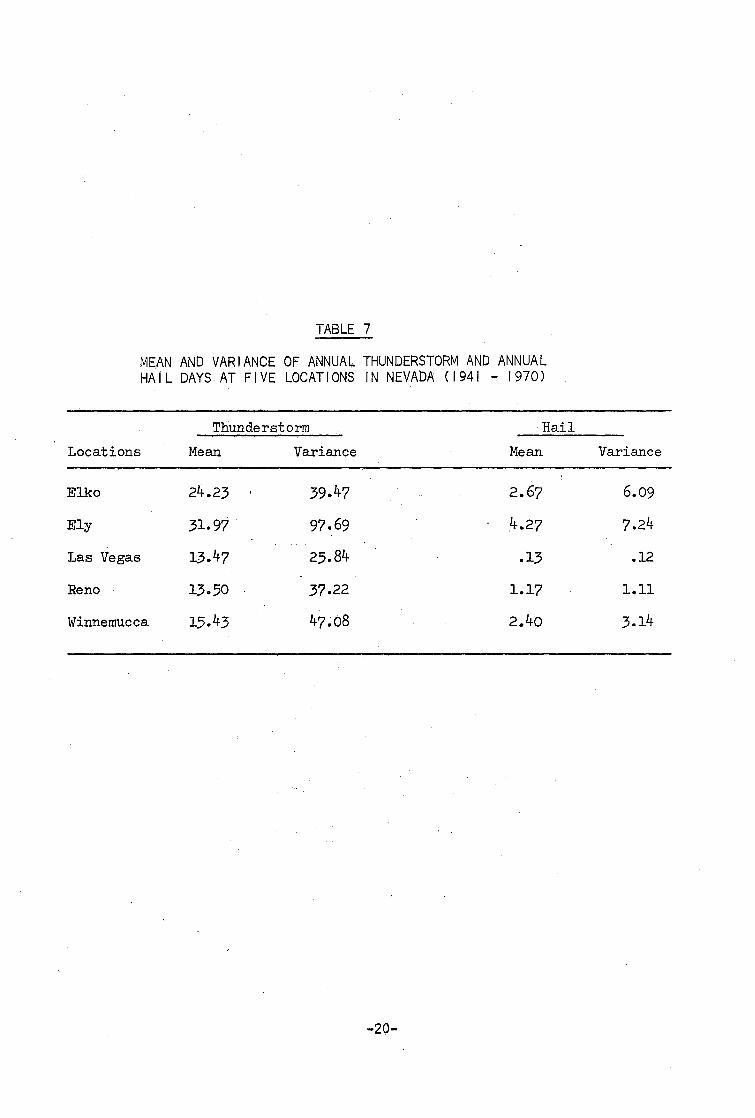
TABLE 7

MEAN AND VARIANCE OF ANNUAL THUNDERSTORM AND ANNUAL HAIL DAYS AT FIVE LOCATIONS IN NEVADA (1941 - 1970)

Thunderstorm Hail

Locations Mean Variance Mean

Elko 24.23 39.47 2.67

Ely 31.97. 97.69 .4.27

Las Vegas 13.47 25.84 .13

Reno 13.50 37.22 1.17

Winnemucca 15.43 47.08 2.40

-20-

Variance

6.09

7.24

.12

1.11

3.14

TABLE 8

CALCULATED (C) AND OBSERVED (0) CUMULATIVE PROBABILITIES OF ANNUAL THUNDERSTORM DAYS AT FIVE LOCATIONS IN NEVADA ( 1941 .,. 1970)

No. LOCATIONS Days ELKO ELY LAS VEGAS RENO WINNEHUCCA

c 0 c 0 c 0 c 0 c 0 0 .000 .000 .000 .000 .000 . • 000 .001 .000 .000 .000 1 .000 .000 .000 .000 .001 .000 .003 .000 .002 .000 2 .000 .000 .000 .000 .002 .000 .009 .000 .007 .;033 3 .000 .000 .000 .000 .007 .000 .021 .000 .017 .033 4 .000 .000 .000 .000 .018 .033 .042 .033 .032 .067 5 .001 0.33 .000 .000 .037 •033 .072 .067 .055 .100

6 ~002 .033 .000 .000 .066 .067 .112 .167 .086 .133 7 .005 .033 .000 .000 .108 .167 .162 .167 .123 .133 8 .010 .033 .001 .• 000 .162 .167 .219 .233 .167 .133 9 .018 .033 .002 .000 .227 .200 .283 .300 .217 .167

10 .030 .033 .003 .000 .300 .367 .349 .367 .272 .233

11 .o48 • 067 .005 .000 .380 .367 . .418 .433 -329 .267 12 .072 .100 .009 .000 .460 .433 .485 -533 .387 ·.333 13 .103. .133 .013 .000 .540 -500 -551 .600 .446 .400 14 .143 .133 .020 .000 .615 .567 '.612 .600 -503 .467 15 .189 .133 • 028 .000 .684 .667 . .669 .633 -558 .467

.l 16 .242 .200 .039 .000 .745 -733 -720 .633 .610 .567 17 .300. .300 .053 .000 -798 .800 -765 .667 .658 • 667 18 .362 .300 .070 .133 .842 .833 .805 .767 -702 .700 19 .426 -333 .090 .133 .879 .867 .839 -799 -743 -733 20 .491 .433 .113 .200 .908 .867 .869 -799 -779 -733

21 -554 -533 .139 .200 ·4931 .• 933 .894 .867 .811 .833 22 .615 .567 .168 .233 .949 .967 .914 .899 .• 840 .867 23 .672 .700 ~200 .267 .963 .967 -932 .966 .865 .900 24. -724 .• 700 .235 -333 -973 1.000 .946 .966 .886 •. 900 25 -770 .800 • 272 -333 . .981 -957 1.000 .905 .900

30 .924 .900 .475 .433 -998 .988 .964 1.000 35 .981 1.000 .667 -533 -997 .987 40 -996 .814 -767 -996 45 .906 -933 50 .942 .967

. 55 .942 1.000

-21-

- - ---- --- ------ -- -- ---- - ------- - --·--·· ---- -------- - ----- --- ------- -------- --------- - -- ------ --- -- - -------- ------------- --

No. Days

0 1 2 3 4 5

6 7 8 9

10

11 12 13 14 15

TABLE 9

CALCULATED (C) AND OBSERVED (.0) CUMULATLVE PROBABI UTI ES OF ANNUAL HAIL DAYS AT FIVE LOCATIONS IN NEVADA (1941 - 1970)

LOCATIONS ELKO ELY LAS VEGAS RENO WINNEMUCCA

c 0 c 0 c 0 c 0 c 0 .16o .100 .044 .000 .875 .867 .311 -333 .091 .100 -370 .300 .147 .100 . -992 1.000 .674 .633 .308 .367 .561 .567 .292 .100 . 1.000 .887 .867 -570 .6oo .'710 -733 .450 .233 .969 1.000 -779 .767 .815 .867 -596 .633 -993 .904 .867 .886 -933 -717 .Boo -999 .964 -933

-931 -933 .809 .833 .988 .967 -959 -933 .876 .867 -997 1.000 -976 -933 -922 .900 .986 .967 -952 -933 -992 .967 -971 .967

-995 1.000 .983 1.000 -990 -994 -997

-22-

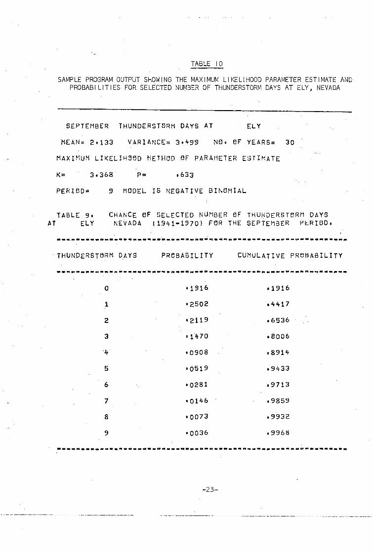
TABLE 10

SAMPLE PROGRAM OUTPUT SHOWING THE MAXIMUM LIKELIHOOD PARAMETER ESTIMATE AND PROBABILITIES FOR SELECTED NUMBER OF THUNDERSTORM DAYS AT ELY, NEVADA

SEPTEMBER THUNDERSTE:lRM DAYS AT ELY

MEAN= 2d33 VARIANCE= 3•'+99 NO• eF YEARS= 30

MAXIMUM LIKELIK~5D METHeD OF PARAMETER ESTIMATE

K= 3o368 P= .633

PER.IE:lD=

TABLE 9• AT ELY

9 MODEL IS NEGATIVE BINE:lMIAL

CHANCE eF SELECTED NUMBER eF THUNDERSTE:lRM DAYS NEVADA (1941•19701 FOR THE SEPTEMBER PtRieDo

THUNDERSTeRM DAYS PROBABILITY CUMULATIVE PR~HABILITY

0 •1916 •1916

1 •2502 ·4417

2 •2119 ·6536

3 •1470 ·8006

"4 •0908 t891't

5 •0519 e9433

6 •0281 e9713

7 •0146 ·9859

8 •0073 ·9932

9 •0036 ·9968

-23-

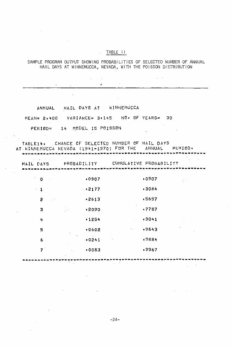
TABLE II

SAMPLE PROGRAM OUTPUT SHOWING PROBABILITIES OF SELECTED NUMBER OF ANNUAL HAIL DAYS AT WINNEMUCCA, NEVADA, WITH THE POISSON DISTRIBUTION

ANNUAL HAIL DAYS AT WINNEMUCCA

~1EAN= 2 • 400 VARIANCE= 3t145 N6• ~F YEARS= 30

PERieD= 14 ~DDEL IS PersseN

TABLE1~• CHANCE eF SELECTED NUMBER eF HAIL DAYS AT WINNtMUCCA NEVADA (1941•19701 F~R THE ANNUAL PEHIElD•

HAIL ~AYS PRElBAfJILITY CUMULATIVE PR6BABILITY

0 •0907 •0907

1 •2177 •3084

2 •2613 o5697

3 •2090 ·7787

4 •1254 •9041

5 •0602 ·9643

6 •02lt-1 e988lj.

7 •0083 a9967

-------~~----------"-~--------------~--·---~---"~------------

-24-

I

rug N Vl I

Sep

Oct

nn

TABLE 12

COMPARISON OF PARAMETER K ESTIMAT6S BY METHOD OF MAXIMUM LIKELIHOOD (MXL), METHOD . OF MOMENTS (MOM) AND "BY EYE" FOR THUNDERSTORM PROBABILITIES IN NEVADA

ELKO ELY LAS VEGAS RENO WINNEMUCCA

MXL MOM EYE MXL MOM EYE MXL MOM EYE MXL MOM EYE MXL MOM EYE

2.228 1.819 2.226 4.013 4.067 4.017 --- --- --- 2.277 3.447 2.273 1.377 1.573 1.366

3-499 3-197 3.497 --- --- --- 1.784 1.739 1-779 2.042 2.560 2.040

3.047 3-927 3.037 --- 6.750 --- 3.060 4.522 3.064 1.8552.361 1.849

3-315 4.735 3.316 5-831 5-474 5.831 2.180 2.614 2.174 1.035 1.109 1.037 1.227 1. 652 1.222

1.833 2.133 1.833 3.368 3-333 3-373 1.704 2.169 1.700 --- --- --- 1.960 2.138 1.956

.840 1.065 .840 .902 L044 .896 .382 • 271 .381 .259 .190 .247 .

--- 24.233 --- --- 15.548 --- 14.652 --- 7.282 7.682 7.282 6.23~ 7.526 6.241

APPENDIX

-26-

FORTRN'~ IV program for computin<1 probabi.l ities of thunderstorm and hai I davs.

1: IMPLICIT REAL~8 (A•H;B•Zl 2: CeMMON XF1~5l,CAI1l,l•PEA114l,PC(551,CPHeB{551•FIN1141

3: DIMENSiflN ARRAY!55•1'1•EVENTI55),CEST(6U,21,XBAR(141,VAR(14l 1 YEARS 4; 1114J,G(3.•3)JH(3)J!N(l41 ~: D!~E~SlflN IPERIODI14J3l,ISITE15,3) 6! DIMENS15N 0~121,ZI31

7: DATA (llPERitJDIKI,JJ,J=1,3l;Kl=1J14l/' JANUARY 11 1 FEBRUARY

8: 2'' MA.RCH '•' APRIL ''' MAY ''' JUNE ,,, 9: 3JUL Y 1 1 1 AUGUST ', 1 SEPTEMSER '1 1 ElCHlBER t 1' NflVEMBER

10: 4 '•' OECEMRER 1 1 1 ANNUAL ''' ANNUAL 'I 11: DATA IIISITEIID,Ll,L=1•3l' ID=l,Sl/' ELY ''' RENr3 ,,, 12: 2 ELKe '•' WINNEMUCCA''' LAS VEGAS 1/ 13: c l't: c 15: c 16: 17: 18: 19: 20: 21: c 22: c 23: 24; 25: 26: 27: 28: 29: 3c: 31: 32: 33: 34: c 35: c 36: c 37: c 38: 39: 4C: 41: 42: 43: c 4-.: 45; 46; 47: 48: c 49: c so: 51: 52: 53: 54: 55: 56; c 57: 58: c 59: c

EVALUATIElN HF X FACTflRIAL

XF(11=0• XF. ( 2) =1 De 300 I=J,ss XXF=l•1

300 XFIII=XF(l•ll~XXF

WRITE1108•510) 510 FfJRMATI2X• 1 PRe!BABILITY ElF THUNDERSTORM AND HAIL DAYS'Jil

WRITE1108•505l 505 FBRMAT(//, 'ABSTRACT: THIS PR0GRAH CALCULATES PROBABILITIES flF MElN

lT~Ly AND AN~UALt~/'THUNbERSTBRM DAYS ANU ANNUAL HAIL DAYS AT FIVE 2L~CATIUNS IN NEVADA! 1 1/ 1 ELY, RENQ, ELKO, WINNEMUCCA AND LAS VEGA 3So ·. TESTS Af-T CCJNDUCTED T0 1 ,/'DETERMINE WHETHER THE POISS(lN CR THE It-NEGATIVE BINOMIAL MCJDEL SHCULD•,/tB~ US~D• EFFICIENT ESTIMATES OF 5CF THE PARAtiETERS ARE CALCULATED BY EITHER•,I•THE METHeO ElF MOMENT 6S OR BY THE METHHD OF MAXIMUM LIKELIH~OU FCJR•,;•THE NEGATIVE B!NBM 71AL •' I

Dt< FOR 5 S IJES

MAIN PR~GRAM BEGINS DC1 70 I.D=1;5 DO 1 !=1,55 DU 1 J=1•1'1

1 ARRAY(!,Jl=O• RlADt105,1001IID,IN FIND FREQUENCY FeR EACH NUMBER eF EVENTS De 2 1"'1,14 IC=IN<Il+1

100 FORMATI2XJ!4,5X,t2t3XJI21•1X,I2,1X•l2) 2 ARRAYIIC,Ilo:ARRAY(ICJII+l•

TEST FOR NEXT LeCATleN 5 READI105J100' END=501 IDD1IN

IFIIID•NE•IDDI GO Te 50 De 3 I=1•14 IC=IN1Il+1

3 A R R A Y ( I C J! l =ARRAY (! C II I + 1 • Gel T e 5 DC FeR MBNTHLY THUNDERSTeRM + ANNUAL THUNDERSTeRM AND ANNUAL HAIL•

50 Dr. 60 Kl=1J14 XX=SUM eF X SQUARES; XB=SUMS OF X; CA=TOTAL N ~R NUMBER eF YEARS INITIALIZE

-27-

60 c 61 62 63 6'+ c 65 c 66 c 67 68 69 70 71 72 73 71+ 75 76 77 78 79 80 81 82. 83: 81t: 85: 86: 87:

c c c

8.8 ': 89: 90: 91: 92: 93: 94': 95: 96. c 97 c 98 c 99 c

c c

100 c 101 c 102 c 103 c 101t c 105 ·- c 106: c

55 XX=O• XB=O• CA=O•

S~LVE FOR SAMPLE MEAN AND VARIANCE

De 6 I=1J55 Xl=I•1 EVENTili=ARRAYIIJKII XX=X~+tVENT!Il•XI•XI XH=Xd+EVENTill•XI

6 CA=CA+EVENT(II

35 108

36

1C:i1

_. 125 (30

475 106

IF !XB•EQ•O) GO TO 35 XBAR!Kll=Xf:l/CA VARIKI)=(XX•XBARIKII¥XB)/(CA•1•l YEARS!Kl l=CA Ge Te 36 WRITE I108J108l!IPERICD!KlJJ)JJ•1J3),(!~ITEIIOJLIJL=1J3) FBRMATI '1 1 ,3XJ3AitJ5XJ3A4J5XJ•NO THUNDER~TORMS'J///1 GO TO 60

CALCULATE PARAMETERS K AND PIK=CAI1 P=P~A) BY METHIJD eF MeMENTS

CAIIKI)=IXBARIKil••2l/IVARIKil•XBARIKill PEAIKII=XBARIKI)/CAIIKI) IFIK!~EQ•1'+1 Ge TO 125 WRITE! 108J 101 l I IPERiflD!KIJJ)JJ=1J3lJ I !SITE! ID,LIJL:s1,31 FeRMAt! •1i12X1jA4, •THUNDERSTORM DAYS AT 1 J2XJ3A4J/) Gd te lt7~ · : · WRiTE ( 1081 13 0 l ·· I I PER HiD I K I 1 J ) 1 J=·t 1 3 ) i· I l ~IT E I I D 1 L I 1 L"' 1 i 3 I . F~RMATI 1 1'J_3XJ3A4J 1 HAIL DAYS ATii2XI3AIIi/l

~RiNt ~tRlOD, L~CA1IriNJ MEAN, VARIA~CE ANb YEARS WRiTE11dS,1b6l ~~A~fRI lJVARIKilJYEARSIKil FORMATI3XJ 'MEAN='Fbo3,3XJ 1 VARIANCE= 1 JFb•3J3XJ'N0• tlF YEARSi:i•JI4dl

SHOULD PIJISSON OR NEGATIVE BTNOMIAL MOD~L BE USED? IF THE CHI•SQUARE VALUE OF DEGREES eF FNEEDOM AT THE o05 LEVEL ~S. EXCEEDEDJ PReCEED TO TEST WHETHER PARAM~TERS K AND P BY METHeD OF MOMENTS IS EFFICIENT• IF NOT EFFICIENT, CALCULATE PARAMETERS BY MAXIMUM LIKELIHU~D METHeD~ IF •05 LEVEL IS N6T EXCEEDED, PROCEED TU P6ISS6N

INITIALIZE

107: N=O 1os: oe 491 I=1,55 109: 491 IFIEVENT!Il•NE•Ol N=I 110: C WRITE11081'+93)N 111: C 493 FfJRM~TI 1 N=•II31 112: XXX=YEARSIKI!•1 113: c 114: c 115: 116: c 117: 118: 119: c

P6LYN6MIAL EQUATI~N RELATING DEG FREED~M WITH CHI•SQUARE VALUES WHY=4o54921+1•41672•XXX•0•00367~4¥(XXX~XXX)

CON=IYEARSIKI)¥XX/XBI•X6 I~(tO~•·GT•WHYl ~6 te 310

-28-

1 ?.0: c 121: c 122: 123: c 124: c 125: c 126: 127: 128: 129: 130: 131:

EVALUATIC.lN 5F Pf.JISSeN. D ISTR IBUT I6N

CCPRtJB=:Q

N CHA~GED Ttl MAXIMUM EVENT NUMBER F~R DO LOOP

N=:55 l!e 325 IX=11N 1IX=IX•1 IFIIIX•E~•Oof:lR•IIX•EQ•ll Ge TO 494 P=IIX-I'DL(JGIXBARtKill~DUlGIXFIIX l )wXBAR!Kil Gel TO 498

132: '194 P=IIX-I'DLtlGIXBARIKil l•XBARIKil P=DEXPIPJ 133: 498

13'+: 135: 136: 137: 32Ei

CC PRflFJ=CCPRelB+P PCIIXJ=P CPReBIIXJ~CCPROB CeNTINUE

138: 139: c l 'tO: C lltl: c 1'<2: c 1Lr3: c 144: c 145: c 146: c 14 7: c 1'18: 1'+9: 1:.o: 151: c 152: c 153: c 154: c 155: c 156: c 157: c 158: c 15Cl: c 160: c 161: c 162: c 163: c 164: 165: 166: 167: 168: 169: 170: 171: 172: 173: c 174: 175: 176: c 177: 178: c 179: c

Gf:l Hl 400

ARE PARAMETERS EFFICIENT? METI-ieD Of. MtJ~IEf~TS VERSUS MAXIMUM LIKELlHeltJD INITAL ESTIMATES eF PARAMETERS ARE Mf:lMENTS ESTIMATtlRS

TEST FOR EFFICIENCY

310 AYE=il•+I1•/PEAtKIJ i J-v-ICAIIKU+2•l IFIIN•2l•EQ•Ol Gtl Ttl 92 1F(AYE•GT•20l GO TO ~2

ESTIMATieN ~F PARAMETERS BY MAXIMUM LIK~LIHe~o METH6D FIND MINIMUM DIFFERENCE BY PARTIAL DIFF~RENTIATieN

D I I =C i\ ( LN ( ( 1 +XB A R) /K ) , M ( ( R ( 1 ) +R ( 2) + ••• +R ( N, I K) + ( R ( 2, +R ( 3+ + ••• +R ( N J/IK+11+!RINl/IK+Z•1l l WHERE: CA=T~TAL NUMBER 5F YEARS N=EVENTS Z=HIGHEST VALUE eF N OBSERVED RiNI=eBSERVED FREQUENCY OF N EVENTS XBAR=K'~-P

CAI=INITIAL MDMENTS ESTIMATE DF K

INTE=:CAIIKII/•05 IFIINTE·GT•30l INTE=30 RA=INTE CAIII=CA!IKil••05-v-RA IFICAIII•LT•Ol CA!!I=•Ol

22 De 16 JK=l160 CAII I=CAIII+•05 Dl=DLOG(l+iXBAR(Kll/CAIIIl) -v-YEARS(KIJ DII=O YEARSIKIJ~NUMBER eF YEARS XBEl=YEARSIKil Ctd I =CA II I K IS New EQUAL TO CAII CESTiJKJ2l=CAll

REDUCE NUMERAT6R BY FREQUENCY eF ARRAY

-29-

180: c 181: 182: 183: 184: c 185: c 186: c 187: 188: 189: 190: 191: c 192: c 193: 194 195 196 197 198 199 200 201 202

c c c c

203. c c

Nt1=N•2 De 15 Icl,NM XE<~=XBB•EVEtH I I l

INC~EHENT DENl'lMINATflR K BY 1 Te K+I•1

DII=DII+(XBB/CAIII to CAII=CAII+1•

DIF=DI•OII CEST(JK,11=DIF ~RITEil08,23l CESTIJK,1!,CEST!JK12)1DI,UII

23 FeRMATI2XJ4F10•5l 16 CeNTINUE

CALL FIND!CEST1MIDDI ISTAR=MIDD•4 ILAST=HIC:D+4 IF!ISTAR•LT•1l ISTAR=1 IF!ILASToGTo60l ILAST=MIDD WRITEI1Q8Jl4) ISTAR,!LAST

14 FHRMAT12X12F10•5)

SEceND eRDER peLYNflMIAL ESTIMATteN flF CGNSiANT AND REGRESSI~N C~EFFICIENTS

oe 17 I=1'3 HI I I =0 De 17 J=113

17 G(I1Jl"0 De 18 K=ISTAR1ILAST Zlll=CESTIK121 Z!2):;Z(l)H2 Z(31=CEST(KJ1 I

c 12345

204: 205: 206: 207: 208! 209: 210: 211: 212! 213: 214: 2Ui: 216: c 217 c 218 219 2?.0 221 222 223 224. 225: c 226: c 227: 228:

WRITEI108112345) Z FCRMAT(3F10•3l

c c

229: c 230: c 231! 232: 233: 234: c 235: c 236: c

De 18 I=11~

SUMS HIII=HIII+Z(II De 18 J=113

CRess PReDUCTS 18 GII,Jl=GII1Jl+Z(II¥Z(J)

De 19 1=113 oe 19 J=113

CeRRECTII.lN TERM KK=IILAST•ISTARI+1

19 GII,Jl=G(I,Jl•(H(Il/KKI.,.H(J) WRITE!108J13) KK

13 FtlRMATI•NI.lo l'lF SAt~PLES=t II3) De 30 1=113 H(II=H(I)/KK

30 CfJNTINUE

MATRIX INVERSiflN

237l CALL MATINV (GJ2,Yl 2381 De 31 1=1,2 2391 f.lK(l)mQ

-30-

240! 241: 2'12: 243: 24 4: c 245: c 246: c 2'17: 248: 249: 250: 251: 252: 253: 254: 255: 256: 257: 25!:1: 259: 260: 261: 262: 263: 264; 265: 266: 267: 268: 269:

c

c

c c c c 278:

279: 280: 281: 282: 283: 284: 285: 286; 287: 288: 289: 290: 291: 292: 293: 294: 295: 296: 297: 29!:1: c 299: c

DO 32 J-=112 32 eKt I l'"'OKII l+G( I,Jl~G(3,J) 31 GelNTINUE

R=HIJl•OK(l)~Hil)•eKI2l¥H{2)

CALCULATION OF REAL VALUES FReM QUADRATIC EQUATieN

D=ABS I I OK I 1) '1''~<2 l •I 4¥!:JK I 2 l ¥R l l DA=DSQRTID! AA;2>;<elK(2l Xl=I•GKill"DAl/AA X2=1"eKC1l+DAl/AA IF1Xl•GT•X2 oANO•X2•GT•Ol Xl=X2 FINIKI l=X1

24 PEAIKil•XBARIK!)/FINIKI) 20 WRITEtl08•21l 21 FCRMATI2XJ 'MAXIMUM LlKELIHeeD NETHeD OF PARAMET~R ESTIMATE 1 ,/l

WRITEI108J102l FINIKil•PEAIKil 102 FeRMATI2X• •K=''Flo•3•5x, •P=••Fto•3l

Gtl HJ 90

'100 110

92

WRITEii08•110l KI FORMATI5X,'PERICD='•I5,2X, 'MODEL IS POISSeN 1 ,//)

oe Te 420 li R I T E ( 1 0 8 1 11 2 )

112 FCRMATI2X••MeMENTS METHOD CF PARAMETER ~STIMATE 1 J//) FINIKil=CAIIKil

114

90

201 420

WRITEt108•114l FINIKil•PEAIKil FeRMATI2XJ 1 K='•Fl0•3,5x,•P=•,5x,F10•3,//)

""

200 WRITEI108•240) K!;IISITEIID,Ll,L=1J3l, llPERIBDIK!,J),J•1,3l 2'10 FORMATI2X•'TABLE'•I2, 1 •'•' CHANCE eF SELECTED NUMBER OF THUNDERS

1HlRM DAySt,jiATtJ3A4•'NEVADA 11941•1970) FeR THE'J3A4•'PERIODoll/ 2)

WRITE I 108•245) 245 FeRMAT(2XJ •·~········-·•••••••···-·-·••••••••••••••••••••••••••••-

1------•,;) I<R ITE ( 1081260)

260 FeRMATI2X;ITHUNDERSTEJRM DAYS PRBBAolLITY 1ILITY 1 ;/l

WRITEI108,245) De 265 IX::l1N IIX=IX"'l WRITEI108J270) IIXJ PCI IXl1CPReB( IXl

270 FeRMAT(10XJI3J15XJF6•4•11X•F6•4J/l IF(CPRf:lBIIXl•GTtt995) GO TC 267

265 CeNTINUE 267 WRITE1108•245)

GEl TEl 60

CUMULATIVE PRBBAB

PRINT PROBABILITY (INDIVIDUAL AND CUMULATIVE) FeR EACH EVENT

-31-

300: 301: 302: 3031 304: 305: 306: 3071 308: 309' 310 311 312 313 314 315 316 317 318 319

1: 2: 3: 4:

c c

5: c 6: c 7: c 8: c 9: c

10: 11: 12: c 13. c 14 15 16 17 18 1~ 20 21 22 23 24 25 261 27' c 28 c 29 c 30

'31 32 33 34 35 c 36. c 37 c 38 39 40 41 42 '+3 '+4 c

HAIL DAYS TABLE

330 wRITEI108•340l Kl•IISITEIID,Ll•L=1•3lJ!lPERIODIKI1Jl•J=1•3l 340 FCRMAT!2X• tTABLE•,I2'''''' CHANCE ~F SELECTED NUMBER OF HAIL DAY

tSt, 1 IAT'•3AI+,tNEVADA !1941•1970) FeR THE 1 •3A41 1 PERIODt 1 l wRITE! 1081245) WRITE! 108•360)

360 FeRMATI2XJ •HAIL DAYS PRf:JBABILITY CUMULATIVE PROBABILITY• l wRITEI108J245l De 365 IX=11N IIX=IX•1 WRITEI108J370l IIX 1PCI !Xl,CPROBI IXl IFICPR6BIIXl•GToo995l GO TO 367

370 FeRMAT!6X1!3•13X•F6•4,13XIF6o4,/) 365 CeNTINUE 367 WRITEI1081245l

60 CBNTINUE 70 CONTINUE

STflP END

SUBROUTI~E NEGO!Nf:J INN1MMl I~PLICIT REAL~8 IA"HJO•Zl CBMMON XFI~5l•CAI114),PEA114l•PCI55l,CPHeBI55l•~INI14l DIME~SlON FFINI55)1FF155l1FKAY!55l NEGATIVE BINOMIAL PROBABILITY FUNCTION I~ NATURAL LO~ARITHM LNIPl=K>,<LNI loll 1+Pl l+LN!FKAYl+IX~LNI IPl/IP+l• l l P=PEAIMMl AND K:F!N(MMI ARE NEGATIVE BlNOMIAL PARAMETERS WHEREIFKAY=(K+X•tlFACTORIAL/X FACTeRIAL"'IK•11 FACTURlAL

De 20 II"t,NN IX=II•l EVALUATt~N OF IK+X•ll FACTORIAL =FF1Nilll

PP=1• IFIIXoEQ•Ol GO TO 15 IF(IX•EQ•1l GO Tel 16 FFIN(Ill=FlNIMMl+IX FFCIIl=PP•FFINIIIl FFINII!l=l• De 18 I=11!I•1 FF IN I I I l =FFI>.J (I I l ~IFF I I I l •I l

18 CtJNTINUE GfJ te 20

15 FFIN!1 l=O 16 IFIIX•EQ•ll FFIN12l=FINIMMl 20 CONTINUE

EVALUATI6N OF Xl STeREO IN CBMMtJN AS XFIIIl

CCPROB=O De 40 II=1,NN IX=If•l IF IIX•EQ•O) GO TO 25 A:iXF!lii

SeLUTlfJN TO FKAY

FKAY!Ill=FFINIIIl/A P=FINIMMl~DLf:lGI1o/l1•+ PEA(MMlll+DLOG!FKAYIII ,-ll+IX¥DLOG! PEAIMMl/

liPEAtMMl+l•l l Ge TO 23

25 P=FINIHMl~DLtJG(1o/l1o+PEAIMMlll 23 P=DEXPIPl

45 C INDIVIDUAL AND CUMULATIVE PR6BABILITY '+6 c '+7 CCPR~B=CCPROO+P 48 CPROBIII l=CCPROB 1+9: PC I I I ) =P 50: 40 CONTINUE 51: 329 RETURN 521 END

-32-

1 : SU,RFJUT H<E MAT!NV!A,N,V) 2: IMPLICIT REAL¥8 (A•H,e"Z) 3: DIHOISltJ~J A(3J3J,V(l) 4: N~~1=N~l

5: DO 776 L=lJN 6: Al1=A(ldl 7: De 774 J=1,Nt11 H: 774 V!Jl=A! l;J+1 )/All 9: V!Nl=l•/A11

10: DEl 779 I=1,NM1 11: IPl=I+l 12: AIP11=A!IP1J1l 13: DEl 775 J=1,t<l'11 14: 775 A!I•Jl=A(lP1,J+1l•AIP11¥V(J) 15: 779 A!I,Nl=•AlP11•V!Nl 16: De 776 J=l1N 17: 776 A(N,Jl=V!Jl 18: f<ETURN 19; END

1! SUBR~UTINE FIND!CEST,Nl 2: IMPLlCll REAL¥8 (A•H,H•Zl 3; DlMENSIElN cEST!60J2l 4: JL=1 5! IF!CEST!ldl•LT•O•l IL=2 6: oe 1 1=2•60 7: IS= 1 !!! IF!CEST!I>ll•LT•O•l IS=2 9: IF!IS•NEdLl N=Il Gel TEl 20

10: N=l 11: 20 RETURN 12: END

-33-

Western Region Technical Memoranda: (Continued)

No. 45/2

No. 45/3

No. 45/4

No. 46

No. 47

No. 48 No. 49

No. 50

No. 51

No. 52

No. 53

No. 54

No. 55

No. 56

No. 57

No. 58

No. 59

No. 60

No. 61

No. 62 No. 63

No. 64 No. 65 No. 66

No. 67

No. 68 No. 69

No. 70

No. 71

No. 72

No. 73

Precipitation Probabilities in the Western Region Associated with Spring 500-mb Map Types. Richard P. Augulis. January 1970. CPB-189434) Precipitation Probabilities in the Western Region Associated with Summer 500-mb Map Types. Richard P. Augul is. January 1970. C.PB-189414) ·Precipitation Probabilities in the Western Region Associated with Fal I 500-mb Map Types. Richard P. Augul is. January 1970. CPB-189435) Applications of the Net Radiometer to Short-Range Fog and Stratus Forecasting at Eugene, Oregon. L. Yee and E. Bates. December 1969. CPB-190476) Statistical Analysis as a Flood Routing Tool. Robert J. C. Burnash December 1969. CPB-188744) Tsunami. Richard A. Augul is. February 1970. CPB-190157) Predicting Precipitation Type. Robert J. C. Burnas.h and Floyd E. Hug. March 1970. CPB-190962) . Statistical Report of Aeroallergens (Pollens and Molds). Fort Huachuca, Arizona 1969. Wayne~. Johnson. April 1970. CPB-191743) Western Region Sea State and Surf Forecasterts Manual. Gordon C. Shields and Gerald B. Burdwell. July 1970. CPB-193102) Sacramento Weather Radar Climatology. R. G. Pappas and C. M. Veliquette. July 1970. CPB-!93347) Experimental Air Quality Forecasts in the Sacramento Val ley. NormanS. Benes. August l 97 0 • C PB-1 94 I 28) A Refinement of the Vorticity Field to Delineate Areas of Significant Precipitation. Barry B. Aronovitch. August 1970. AppliCation of the SSARR Model to a Basin Without Discharge Record. Vail Schermerhorn and Donald W. Kuehl. August 1970. CPB-194394). Areal Coverage of Precipitation in Northwestern Utah. Philip Wil Iiams, Jr., and Werner J. Heck. September 1970. CPB-194389) Preliminary Report on Agricultural Field Burning vs. Atmospheric Vtsibil tty in the Wi llamette Valley of Oregon. Earl M. Bates arid David 0. Chilcote. September 1970. CPB-194710) Air Poi lution by Jet Aircraft at Seattle-Tacoma Airport.· Wallace R. Donaldson. October 1970. CCOM-71-00017) Application of P.E. Model Forecast Parameters to Local-Area Forecasting. Leonard W. Snel lman. October 1970. CCOM-71-00016)

NOAA Technical Memoranda NWS

An Aid for Forecasting the Minimum Temperature at Medford, Oregon. Arthur W. Fritz, October 1970. (COM-71-00120) Relationship of Wind Velocity and Stability to so2 Concentrations at Salt Lake City, Utah. Werner J. Heck, January 1971. CCOM-71-00232) Forecasting the Catalina Eddy. Arthur L. Eichelberger, February 1971. (COM-71-00223) 700-mb Warm Air Advection as a Forecasting Tool for Montana and Northern Idaho. Norris E. Woerner. February 1971. CCOM-71-00349) Wind and Weather Regimes at Great Fa I Is, Montana. Warren B. Price, March 1971. Climate of Sacramento, California. Wilbur E. Figgins, June 1971. CCOM-71-00764) A Preliminary Report on Correlation of ARTCC Radar Echoes and Precipitation. Wilbur K. Hal I, June 1971. CCOM-71-00829) Precipitation Detection Probabilities by Los Angeles ARTC Radars. Dennis E. Ronne, July 1971. (COM-71-00925) A Survey of Marine Weather Requirements. Herbert P. Benner, July 1971. CCOM-71-00889) National Weather Service Support to Soaring Activities. ElI is Burton, August 1971. CCOM-71-00956) Predicting Inversion Depths and Temperature Influences in the Helena Val ley. David E. Olsen, October 1971. CCOM-71-01037) Western Region Synoptic Analysis-Problems and Methods. Philip Wi I Iiams, Jr., February 1972. A Paradox Principle in the Prediction of Precipitation Type. Thomas J. Weitz, February 1972. A Synoptic Climatology for Snowstorms in Northwestern Nevada. Bert L. Nelson, Paul M. Fransiol i, and Clarence M. Sakamoto, February 1972. CCOM-72-10338)