NODAL DISTRIBUTION STRATEGIES FOR

DESIGNING AN OVERLAY NETWORK FOR

LONG-TERM GROWTH

By

SUSAN JEAN CHINBURG

Bachelor of Science Minnesota State University, Mankato

Mankato, MN 1972

Masters of Science

San Jose State University San Jose, CA

1985

Submitted to the Faculty of the Graduate College of the

Oklahoma State University in partial fulfillment of

the requirements for the Degree of

DOCTOR OF PHILOSOPHY December, 2006

ii

NODAL DISTRIBUTION STRATEGIES FOR

DESIGNING A CARRIER NETWORK FOR

LONG-TERM GROWTH

Dissertation Approved:

Dr. George Scheets

Dr. Mark Weiser

Dr. Ramesh Sharda

Dr. Rick Wilson

Dr. A. Gordon Emslie

Dean of the Graduate College

iii

ACKNOWLEDGEMENTS

The initial question that began this work was suggested by Chris Hamilton, who when he

posed the question, was Chief Architect of the Optical Network Architecture group at

WilTel, Inc in Tulsa, OK. Chris’s insightful question about how to plan the next

generation of optical network topology was the beginnings of this endeavor.

Dr. George Scheets of the Electrical and Computer Engineering Department in the

College of Arts and Sciences served as the research advisor for this study and has my

undying thanks and gratefulness for supporting me through this entire process. I would

also like to acknowledge the support of the MSIS Department and Dr. Rick Wilson for

supplying the MPS software from Maximal, Inc. Dr. Mark Weiser served as my

committee chairperson and Dr. Ramesh Sharda helped me with the linear program and

the MPL implementation.

The author of this study gratefully acknowledges the support and dedication given her by

her husband, Steven Locy, and her daughter, Jennifer Locy. Without their support this

research and degree would have not been possible. This work is dedicated to them.

iv

Table of Contents

ACKNOWLEDGEMENTS............................................................................................... iii Table of Contents............................................................................................................... iv Table of Figures and Tables.............................................................................................. vii Chapter One Introduction ................................................................................................... 1 Chapter Two Literature Review.......................................................................................... 4

Optimization and Network Design ................................................................................. 4 General Linear Programming Problem Statement...................................................... 5

I. Facilities Location or Node Placement........................................................................ 6 Summary..................................................................................................................... 8 I. Facilities (or Node) Location................................................................................... 9

II. Network Design (link location and capacity).......................................................... 10 Design Principles ...................................................................................................... 10 Multi-commodity Flow............................................................................................. 13 Heuristic Techniques ................................................................................................ 15

Tabu Search .......................................................................................................... 15 Genetic Algorithms............................................................................................... 16 Lagrangian heuristics ............................................................................................ 17 Other Approaches ................................................................................................. 18

Summary................................................................................................................... 19 Network Design Problem Formulation................................................................. 20

III. Multi-level or Hierarchical network design............................................................ 21 III. Multi-level (or Hierarchical) Network Design Problem................................. 28

Summary................................................................................................................... 29 IV. Multi-period Design Approaches that include Growth .......................................... 29

IV. Multi-period Design Problem......................................................................... 31 Summary................................................................................................................... 32

Efficient or Production Frontier.................................................................................... 32 Traffic models and projections ..................................................................................... 33 Summary....................................................................................................................... 35

CHAPTER 3 MATHEMATICAL MODEL..................................................................... 37 Mathematical Model ..................................................................................................... 37

Overlay Switch Cost = Overlay Chassis Cost + Overlay Port Cost ......................... 38 Overlay Chassis Cost ............................................................................................ 38 Individual Overlay Chassis Cost........................................................................... 39 Total Overlay Chassis Cost................................................................................... 40

v

Overlay Port Costs ................................................................................................ 40 Individual Overlay Switch Port Costs................................................................... 41 Total Overlay Port Cost ........................................................................................ 42

Overlay Link Costs ................................................................................................... 42 Individual Overlay Link Costs.............................................................................. 43 Total Overlay Link Costs...................................................................................... 44

Total Cost of a New Service Overlay on a Legacy Network.................................... 44 Cost Relationships .................................................................................................... 46

Network Design Heuristics For Choosing Locations Of New Service Overlay Switches On A Legacy Topology ................................................................................................ 50

Heuristic 1 - Locate overlay switches at nodes in a centralized location of the legacy network ..................................................................................................................... 51 Heuristic 2 - Locate overlay switches at legacy node locations with high connectivity............................................................................................................... 52 Heuristic 3 - Locate overlay switches at legacy nodes with high traffic flow demands................................................................................................................................... 53 Backhaul of Traffic Flow.......................................................................................... 54 Examples of Heuristics ............................................................................................. 55

Summary....................................................................................................................... 62 Chapter 4 Experimental Methods ..................................................................................... 64

Service Overlay with Growth Problem [SOGP] Formulation ...................................... 64 Plan of Analysis ............................................................................................................ 68

Step 1: Legacy topology, T0..................................................................................... 68 Step 2: Traffic Matrix, TMt....................................................................................... 71 Step 3: Cost Models .................................................................................................. 72 Step 4: Develop “Best” network topology............................................................... 73 Step 5: Analyze the impact of nodal distribution – create efficient frontiers .......... 74

Summary....................................................................................................................... 75 Chapter 5 Results of Case Studies Analyses..................................................................... 76

Growth Studies - Scalability ......................................................................................... 77 The 9-node Case Study ................................................................................................. 78 North American and NSFNet Case Studies .................................................................. 82 Summary....................................................................................................................... 96

Chapter 6 Summary and Future Research ........................................................................ 98 Summary....................................................................................................................... 98 Future research............................................................................................................ 100

Reference List ................................................................................................................. 102 APPENDICES ................................................................................................................ 108

Appendix A Network Details...................................................................................... 109 North American Network ....................................................................................... 110

Node #................................................................................................................. 110 Links ................................................................................................................... 111

Pan European Network ........................................................................................... 113 Nodes .................................................................................................................. 113 Pan European Links ............................................................................................ 114 NSFNet Node #................................................................................................... 115

vi

NSFNet Links ..................................................................................................... 116 Appendix B Traffic Matrix ......................................................................................... 117 Appendix C MPL SOGP Implementations................................................................ 153 Appendix D – Skewness calculations ......................................................................... 156

VITA................................................................................................................................... 1

vii

Table of Figures and Tables

Figure 1 Cost function for the overlay switch chassis……………………………..….…39

Figure 2 Connection or port cost model.………………………….……………...……...41

Figure 3 Overlay link cost………………………………………………………………..43

Figure 4 Cost functions where overlay

Link Unit, KL, Costs >> overlay Switch Unit Costs, KS .….……………...…….47

Figure 5 Overlay Link Unit KL costs << Overlay Switch Unit KS costs...………..….….48

Figure 6 Overlay Link Unit KL Cost ≈ Overlay Switch Unit KS Cost. ..………….….….49

Figure 7 Backhaul of traffic flow to an overlay switch…….…………………..….....….55

Figure 8a Centralized versus periphery overlay switch location………………….…..…56

Figure 8b Centralized versus periphery overlay switch location………………….…..…57

Figure 9 (a & b) Locating overlay switch………………………………..………….…...59

Figure 9 (c & d) Locating overlay switch………………………………..………….…...60

Figure 10 – Initial 9 node proof of concept model. ……………………………………..68

Figure 11 The North American legacy topology..……………………………………….69

Figure12 The NSFNet legacy topology....……………………………………………….70

Figure 13 Pan-European legacy topology……………………………………………..…70

Figure 14 Backbone design strategies using logical links or legacy links……………….77

Figure 15 Experimental Total Cost results for the 9-node legacy network……...………80

Figure 16 Switch verses Link Costs……………………………………………………...83

Figure 17 North American Legacy Overlay Design studies. ……………………...……85

Figure 18 NSFNet Legacy Overlay Design studies..……….……………………………86

Figure 19 One-switch one node design total costs verses connectivity of legacy node…89

Figure 20 Pan-European Legacy Network overlay design studies..….……………….…94

Table 1 Network characteristics of the case study designs……...……….………………79

1

Chapter One Introduction

Growth of telecommunications during the 1990’s was driven by the explosive

development of the Internet. During this time, many totally new networks were built, but

in today’s economic climate, new investments will be focused towards getting the

maximum from existing infrastructure. Also being able to plan from the beginning

network designs that can cost-effectively adjust to changing traffic is important (Birman,

2001). The ability of network architecture to adjust and grow to handle increased

volumes of traffic and diverse Quality of Service, QoS, or be scalable, is an important

feature in network design. One factor affecting the scalability of a network is the design

of the physical network topology. The number, size, and arrangement of the nodes and

links in the directed graph that represents the physical network describe the physical

topology. Much research has been done to create methods to help design the optimal or

best network graph with respect to cost (for example; Grover and Doucette 2001,

Gendron, et.al. 1999, Chang and Gavish 1993) but in general the research has focused on

one design period, not long term growth, and finding one “best” design. Also in the area

of large wide area networks (WANs), optimization research has focused on minimizing

the inter-nodal cost function, which is the set of costs associated with the links and the

size of the links connecting the given nodes that will deliver the required traffic demands.

While the nodal distribution strategy, called the node placement or facilities location

problem, has received much attention in many disciplines, it has received somewhat less

2

attention for WAN design. Nodal distribution strategies affect the number, size and

location of nodes in the network. Usually these problems require heuristic algorithms for

sub-optimal solutions because this problem has been shown to be NP-hard and intractable

(Yeung and Yum 1998 and Banjeree, Mukherjee and Sarkar 1994). Most of the previous

nodal distribution research has focused on determining the “optimal” distribution of

nodes for any given network state and thus examined only one nodal distribution pattern.

Scalability, or the long-term growth potential, of nodal distribution strategies has not

been examined extensively nor have comparison studies of different distribution

strategies been done. Additionally, examining the nodal distribution strategies of an

overlay on top of existing underlying legacy network have not been extensively examined

other than as hierarchical or multi-layered networks. The research project presented in

this paper will examine the impact of the nodal distribution strategy of a new service

overlay on a legacy network and will examine the impact of changes to the optimal

design. Specifically, this study will examine and compare long term costs of nodal

distribution strategies that deploy a service using switches in numerous locations with

minimal backhaul of traffic [the distributed approach] to the strategy of using switches in

a limited number of locations resulting in more backhaul of traffic [the centralized

approach]. The key question for this research is the impact of the number of nodes in a

new service overlay. In other words, “Which is better, a service overlay with fewer

larger switches or smaller switches distributed throughout the network? Examples of

scenarios that this problem describes include deploying a VoIP service over an IP

network, deploying an ISP backbone over an ATM network, deploying an ATM

3

backbone over a SONET network, or more generally, deploying a new layer of the some

type of service over an older existing network.

Typically, in network design optimization a methodology is created to define the

“optimal” or best solution depending upon the constraint parameters to be considered.

There is a broad breath and depth of research available to assist in the decision of the

optimal design. All too often after the optimal design has been defined, operational

considerations that were not known during the optimization process pop up and force the

final network design to be changed. One way to understand the impact of change to the

final design and cost structure is to create an efficient or production frontier for that

network problem (Fare, Grosskopf, and Knox Lovell, 1994). The efficient frontier or

production frontier process defines the optimal mix of parameters that will create the

most efficient use of resources for the given problem. By examining the efficient frontier

for any given legacy network topology the impact of change can be examined from many

perspectives.

The remainder of this dissertation is structured as follows. In Chapter Two, a review of

previously published research of nodal distribution, efficient or production frontier, and

problem solution methods is presented. Chapter Three will be a review and analysis of

the mathematical model presented in this study. The experimental methods used to

analyze the case studies will be reviewed in Chapter Four. Chapter Five will be a

presentation of results and interpretation. Chapter Six will be a summary including future

research.

4

Chapter Two Literature Review

Chapter two of this paper will review published literature relating to designing of

telecommunications networks and long-term growth of networks. Network design is the

process of describing the form and function of the network so that day-to-day

functionality happens. Robert S. Cahn (1998) in his book Wide Area Network Design:

Concepts and Tools for Optimization makes the statement “In network design there are

no clear winners, only clear losers. The design process is at its heart the solution to an

ill-defined problem” (p. 2). Network design optimization problems related to this study

are grouped into four categories, I. facilities (or node) location, II. link design including

location and capacity, III. multi-level or hierarchical network design and IV. multi-period

design approaches that include growth. The appropriate network design optimization

literature grouped by the above-described categories will be presented and reviewed. In

each group a representative LP formulation for each problem will be presented. Then the

efficient frontier or production frontier process, a concept borrowed from finance,

agriculture economics, and operations research literature will be reviewed. Another topic

that is important to designing and modeling networks is traffic modeling and it will be

discussed last.

Optimization and Network Design

This section of this paper will review some methods used in published research relating

to network design optimization as it relates to network scalability and design. While this

5

is a lengthy review section, it is by no means an exhaustive review of optimization and

the techniques relating to network design. The intent is to give an overview of the

general area presenting first a general overview of the techniques used to find “optimal”

solutions for network design problems and then second present the specific linear

programming problems that will be used in this study. Mathematical modeling and

optimization are well-developed and mature areas of research with a variety of articles

available for the interested reader who is referred to Bertsekas (1998), Sanso and Soriano

(1999), and Grover and Doucette (2001) for broader overviews.

To find the optimized design, an exhaustive analysis must examine every possible

combination of all parameters thereby proving the best fit to meet the specified design

characteristics. Very quickly, these types of problems become NP-hard and intractable

especially when examining communication networks. Finding near-optimal solutions

requires faster heuristic algorithms, establishing acceptable constraints or bounds and

then “relaxing” these constraints so the solutions can be found with reasonable resources

and time. The bulk of published research and literature deals with ways of making this

very complex problem simpler and easier to solve.

General Linear Programming Problem Statement

General linear programming (LP) techniques are widely used to define optimal

telecommunication network designs to meet one or more parameters. One way to state

this problem is as a general topology design and capacity expansion problem. The

formulation presented by Chang and Gavish (1993) and many others since will be the

format of this paper.

6

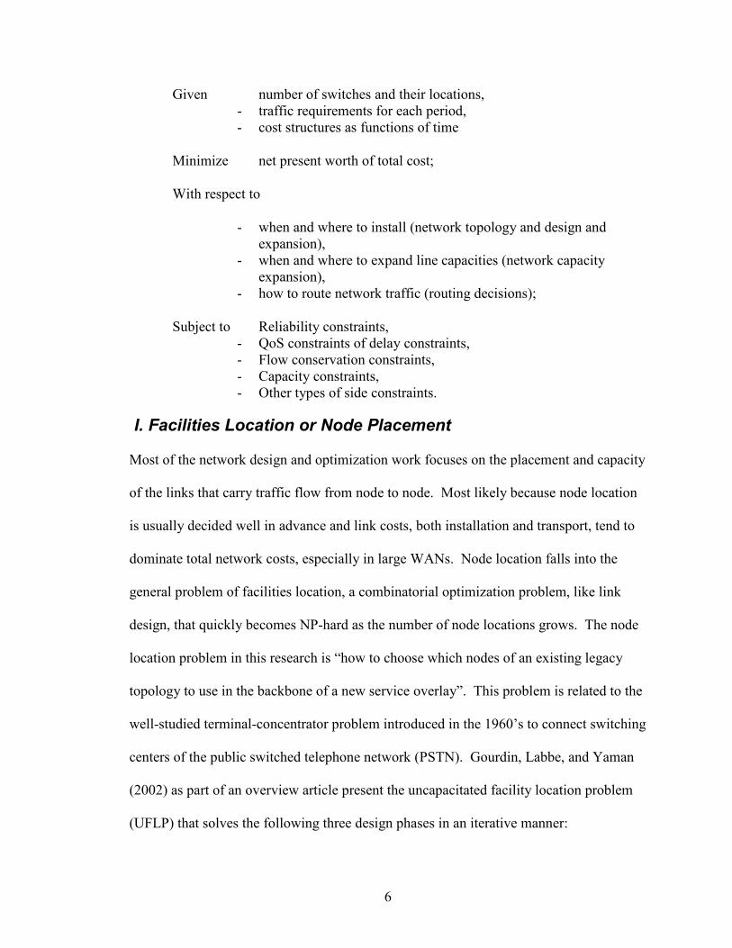
Given number of switches and their locations, - traffic requirements for each period, - cost structures as functions of time

Minimize net present worth of total cost;

With respect to

- when and where to install (network topology and design and expansion),

- when and where to expand line capacities (network capacity expansion),

- how to route network traffic (routing decisions);

Subject to Reliability constraints, - QoS constraints of delay constraints, - Flow conservation constraints, - Capacity constraints, - Other types of side constraints.

I. Facilities Location or Node Placement

Most of the network design and optimization work focuses on the placement and capacity

of the links that carry traffic flow from node to node. Most likely because node location

is usually decided well in advance and link costs, both installation and transport, tend to

dominate total network costs, especially in large WANs. Node location falls into the

general problem of facilities location, a combinatorial optimization problem, like link

design, that quickly becomes NP-hard as the number of node locations grows. The node

location problem in this research is “how to choose which nodes of an existing legacy

topology to use in the backbone of a new service overlay”. This problem is related to the

well-studied terminal-concentrator problem introduced in the 1960’s to connect switching

centers of the public switched telephone network (PSTN). Gourdin, Labbe, and Yaman

(2002) as part of an overview article present the uncapacitated facility location problem

(UFLP) that solves the following three design phases in an iterative manner:

7

1. the number and locations of concentrators and the assignment of terminals to

these concentrators

2. the access networks

3. the backbone network.

Designing large-scale extensive computer networks very quickly becomes an intractable

problem and must be subdivided into multiple steps. Many methods to subdivide the

problem have been presented. Pirkul and Nagarajan (1992) presented a design for a

tree/star network using a two-phase algorithm. A first step sweep phase divides the set of

nodes into regions. The second step formulates a path for each node within a region to

the central node via point-to-point links. Thus, a star design is created within each

region. The central node becomes a node on the backbone and the backbone nodes are

connected. Gavsih (1982) presented formulations of the terminal/concentrator problem

using multidrop capacitated links and expanded the formulation in 1992 so that no apriori

knowledge of the network topology was needed. These two works are often used as the

basis for additional advanced formulations.

Balakrishnan, Magnati, and Wong (1995) developed a formulation that installed

concentrators and expanded the size of links with minimum cost based on a

decomposition method using Lagrangian Relaxation and dynamic programming. Yeung

and Yum (1998) examined node placement using a ShuffleNet graph structure. They

proposed a “gradient algorithm” that minimizes the average internodal hop distance.

Other work examining node placement presented by Ali (2002) examined the

optimization of multicast node in wavelength-routed all-optical networks. This heuristic

8

method examined the location of nodes and developed a near-optimal design using

blocking probability as the performance metric. Murkherjee et al (1996) using virtual

topologies combined subsets of all the nodes and links in the physical topology to

develop optimal or near optimal WDM network design. Chamberland, Sanso, and

Marcotte (2000) using a dual-based heuristic that yielded near-optimal designs, proposed

a solution to the design problem of the appropriate switches for core network nodes.

They proposed a mixed 0-1 linear programming model that includes the location of

switches, the configuration of the switches, ports, and multiplexers, the design of a star

topology access network and a backbone network of a fixed ring or a tree topology.

Using a greedy heuristic to provide a good starting point and a Tabu search heuristic to

improve the solution, a final solution was proposed that would minimize the total cost of

the network. The problem involves selecting the switch sites, the type of ports to be

used, selecting the multiplexers, connecting the users to the switches through OC-3 links,

and interconnecting the switches through OC-192 links in a specified topology. For a

more comprehensive overview of the facilities location problem the reader is referred to a

text by Drezner and Hamacher (2002) which contains a compilation of mainstream

facilities location topics relating to many disciplines with extensive up-to-date reference

lists at the end of each chapter

Summary

Much work has been done, as highlighted in the previous section, in terminal

concentrator (node or switch) design and node connection to centralized concentrators

that designs optimal or near-optimal connections of all the nodes in the physical

9

topology. The limitation as far as this research is concerned is that the location of the

concentrators is usually decided in advance. Once the location or identification of the set

of concentrators has been accomplished there are many formulations for solving this

problem.. The following discussion presents an example chosen because either it was the

most recent example of that problem or it was often cited in published literature.

I. Facilities (or Node) Location

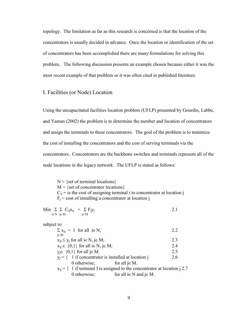
Using the uncapacitated facilities location problem (UFLP) presented by Gourdin, Labbe,

and Yaman (2002) the problem is to determine the number and location of concentrators

and assign the terminals to these concentrators. The goal of the problem is to minimize

the cost of installing the concentrators and the cost of serving terminals via the

concentrators. Concentrators are the backbone switches and terminals represent all of the

node locations in the legacy network. The UFLP is stated as follows:

N = {set of terminal locations} M = {set of concentrator locations} Cij = is the cost of assigning terminal i to concentrator at location j Fj = cost of installing a concentrator at location j

Min Σ Σ Cijxij + Σ Fjyj 2.1 i∈N j∈M j∈M

subject to: Σ xij = 1 for all i∈N; 2.2 j∈M

xij ≤ yj for all i∈N, j∈M; 2.3 xij ∈ {0,1} for all i∈N, j∈M; 2.4 yj∈ {0,1} for all j∈M. 2.5 yj = { 1 if concentrator is installed at location j 2.6 0 otherwise; for all j∈M. xij = { 1 if terminal I is assigned to the concentrator at location j 2.7 0 otherwise; for all i∈N and j∈M.

10

Equation 2.1 is the objective statement to minimize cost. Constraints 2.2 and 2.4 state

that each terminal should be assigned to exactly one concentrator and constraint 2.3 is so

that a terminal can be assigned to a concentrator only if this concentrator is installed.

UFLP is the first phase of an iterative design approach that would feed into the next

phase of the access and backbone design.

II. Network Design (link location and capacity)

This section will examine the area of designing link configuration of the core or

backbone networks that provide transport. Not being constrained by existing ring

topologies, the design of new mesh optical networks took advantage of state-of-the-art

optical switches that pushed optical network technology development. Since this area is

so broad, the literature reviews will be grouped into the following sections; design

principles, multi-commodity flow problems, and heuristic adaptations.

Design Principles

A common network design scheme defines networks around several parameters grouped

into three categories, cost, QoS, and reliability (Cahn 1998). Cost includes

implementation and maintenance. QoS groupings describe the type of services that are

offered by this network and therefore a potential revenue metric. Reliability refers to the

network’s ability to recover from a failure. All three of these parameters while being

distinctly different do interact with each other and can negatively influence each other so

therefore must be balanced against each other. QoS and reliability impact the cost of the

11

network because when those factors are measured or put into the design criteria the cost

of the network increases.

Seven characteristics are often used to guide network design; capacity, scalability,

modularity, upgradability, flexibility, reliability, universality, and transparency

(Dumortier, Masetti, and Sotom 1995). High capacity in any new design accommodates

not only the known traffic but also future needs. Broadband applications will require

increasing amounts of bandwidth and more and more users will demand more bandwidth.

Scalability of a design requires that the network be able to grow gracefully to

accommodate increasing demands. Modularity demands that the design be simple

enough so that the network is constructed of a relatively small number of elements that

can be used to deploy nodes and links in a large size range. Upgradability characteristics

are those that will allow the network to evolve without frequent substantial investments

due to incompatibility of new versions with previously installed network base. Changing

traffic demands are a reality of network life and network design must show flexibility to

accommodate these inevitable changes. Reliability of a network means among other

things that the network can recover from failures (in other words, has built-in protection)

with a minimum amount of delay (has speedy restoration capabilities). Any good

network design requires that the network be capable of supporting a wide range of

services, both current and future, supporting the universality of digitized information

flow. Transparency, in and of itself, is not a design requirement but is necessary to

support universality and other modularity requirements. Networks, ideally, should be

able to accommodate a variety of applications without each application being impacted

by the other. In other words, applications using the network should be transparent to

12

each other. All of these factors impact the cost of the network. Increasing any factor will

increase the cost.

The MENTOR algorithms presented by Cahn (1998) and Kershenbaum et al (1991) are a

heuristic approach using three parameters, weight, radius, cost, that can be adjusted to

define and design, backbone and access to the backbone. By directing the design

development with three principles, first, the shortest path is usually the lowest cost,

second, links should have high utilization, and third, use long high capacity links when

ever possible, the MENTOR algorithms develop a near-optimal or very good design

solutions. Design optimization routines are usually complex and require simplification

modifications to allow the solution to be found with reasonable computing times.

Heuristic approaches such as MENTOR are commonly used in practice to develop

network designs due to the relative simplicity and ease of use. The solutions, while not

necessarily optimal, are usually “good enough” especially when realistically constrained.

MENTOR can also be used for a multi-layer hierarchical design problem.

Grover and Doucette (2001) presented a 1-0 mixed integer formulation of the complete

mesh-restorable topology design with a three stage process for topology planning and

growth of optical mesh networks called mesh topology routing and sparing, MTRS.

Their heuristic solves “three problems (W1, S2 and J3) of reduced complexity to

approximate an optimal single-stage solution to MTRS. W1 finds a fixed charged plus

routing, FCR, type minimal topology and capacity solution as justified by working flows

alone. S2 finds a min-cost topology augmentation as justified by restorability

considerations alone. J3 revises the working flows of W1 to exploit the augmented

13

topology of S2 and coordinates them with the assignment of restoration capacity and

selection of edges to minimize the total cost of realization” (Grover and Doucette 2001).

The union of the three edge sets allows the high quality approximation of MTRS. Each

of these three problems are NP-hard in themselves and combined would be even more

difficult to solve but creating a 3 stage approach allows the problem to be solved. The

union of the three sets creates an effective topology space to solve a restricted instance of

the full problem.

Multi-commodity Flow

The multi-commodity flow problem involves “a collection of several networks whose

flows must independently satisfy conservation of flow constraints” (Bertsekas 1998, p.

349). Associated with the directed graph of the network topology will be a collection of

flow vectors of different traffic values. The sum of traffic flows on each arc (or link) of

the graph is used to define capacity. Saniee (1996) reported a multi-commodity flow

formulation for the routing of traffic problem that achieved maximum network

throughput with minimum blocking loss due to a single switch failure. Girard and Sanso

(1998) reported a multi-commodity flow model applied to the design of circuit-switched

networks with reliability constraints. The results showed that this approach compared

favorably with other exact dimensioning algorithms in use at the time, especially when

failures were considered. Hadjiat, Maurras, and Vaxes (2000) presented a primal

partitioning technique for single and non-simultaneous multicommodity flow problems.

Their use of a simplex-based algorithm modified by a refined primal partitioning to speed

it up, presented a cost effective solution to the design of the French national

14

telecommunications network. Mateus and Franqueria (1998) considered an integer

programming formulation with a partial multicommodity structure to model and define a

generalized access network design problem that connects every remote unit to its central

node in a telecommunications network.

Bienstock and Saniee (2001) updated the multi-commodity flow approach to propose a

methodology for designing ATM networks with the relatively newly proposed Brownian

motion model to define data traffic flows. The multi-commodity problem can be difficult

due to three aspects, 1) the large number of different but interrelated capacity decisions

with rapidly changing cost profiles; 2) the complicated nature of the paths used for

routing, and the potentially very large size of the formulation; and 3) the complexity of

defining the nature of data traffic. This problem is also often plagued with a very large

duality gap and can be presented in large, difficult and ill conditioned linear programs.

The heuristics defined by this formulation were generally good in that solutions were

within 10% of the lower bound or optimal solution for 75% of the test cases. The

solutions were generally independent of the numerical values of the input data, ran in the

magnitude order of tens of seconds, were more dependent on node variables than link

variables and the path generation step had greater impact in constraining the solutions

than previously thought. In general, Bienstock and Saniee (2001) found that the addition

of statistical multiplexing could significantly reduce networking costs in the range of 10-

40% over other approaches.

15

Heuristic Techniques

Many researchers have proposed using heuristic local search techniques as an approach to

solving these NP-hard network design problems. The following section will review Tabu

search, general genetic algorithms, Lagrangian heuristics, and other approaches.

Tabu Search

To avoid being trapped in a less than optimal local minimum, the Tabu search approach

allows accepting a worse or even infeasible solution from within the current

neighborhood to continue the search for the better solution. A list of recently obtained

solutions is maintained in a forbidden (Tabu) list (Bertsekas 1998).

Lee et al (2000) proposed a methodology to find an optimal capacity allocation so that

the total cost of ATM switch modules is minimized. First, they formulated the integer-

programming model as a bin-packing problem with capacity constraints. Then they

developed a Tabu search heuristic that was restricted by tight lower bounds. Their results

show that this type of approach provides good structure for configuring an ATM switch.

Shyur, Lu, and Wen (1999) also presented a formulation of the spare capacity planning

for network restoration using Tabu search. The results from their uphill and downhill

procedures in the neighborhood structure exhibited better performance than other

approaches they compared. Their results showed similar or better spare capacity/working

capacity ratios than random problem experiments.

16

Genetic Algorithms

A group of techniques inspired by real-life processes of genetics and evolution called

genetic algorithms can define neighborhood generation mechanisms (Bertsekas 1998).

An existing solution is modified by “splicing and mutation” to obtain neighboring

solutions. Initially, the methodology solved the traveling salesman problem that attempts

to define the “best” method for traversing a collection of nodes. These approaches are

problem-dependent and require a lot of trial and error but can be quite easy to implement

according to Bertsekas (1998).

The literature regarding the application of genetic algorithms to telecommunication

networks is rich and abundant and the following are a few of the reports using genetic

algorithms. These were chosen to reflect the variation in use of this technique as well as

the development of the application of this technique. Celli et al (1995) developed genetic

algorithms to help optimize the design of the Italian national telephone system to develop

B-ISDN services. Kumar et al (1995) applied genetic algorithms to the solution of

various problems in the design of computer local area networks as compared to

centralized systems. Dengiz et al (1997) developed genetic evolutionary algorithms to

aid in the design of computer networks but added reliability as a design constraint.

Garcia, Mahey, and LeBlanc (1998) presented a new generic auto-calibrating local search

algorithm combined with a genetic algorithm to address multiperiod network expansions.

Cheng (1998) used genetic algorithms to aid Kerbache and MacGregor in the design of

backbone network layouts to define a more cost effective or reliable layout. Sayoud et al

(2001) presented the development of a variation called steady state. This application

17

minimizes the total installation cost of a telecommunications network by designing an

optimal topology and assigning needed capacities. This approach included the option to

terminate the procedure early with a reasonable good solution that satisfied feasibility

requirements. Kumar et al (2002) put forth a multi-objective genetic algorithm procedure

to define a network set-up while minimizing network delay and installation cost that were

subject to reliability and flow constraints. To add QoS constraints to the development of

an Industrial Ethernet network, Krommenacker et al (2002) proposed a genetic algorithm

approach for the optimization and design of industrial control networks.

Lagrangian heuristics

Another area of great interest to researchers in optimization is defining the heuristics used

to solve the NP-hard problem. Lagrangian heuristics or relaxations are an approach for

obtaining the lower bounds to use in the branch-and-bound method (Bertsekas 1998). “A

key idea of Lagrangian relaxation is the minimization of the Lagrangian L (x, µ) over the

set of remaining constraints that yields a lower bound to the optimal cost of the original

problem” (Bertsekas 1998, p. 493).

Pirkul and Gupta (1997) presented a topological design of centralized computer networks

using a Lagrangian heuristic that solved the problem with gaps of 2.7% to 10.4% of the

lower bound using a predefined number of concentrators. This type of approach may be

applied to the design of access layers of networks. Holmberg and Yuan (1998) presented

a common solution approach to solve fixed charged network design models, capacitated

or uncapacitated, directed or undirected. They proposed a Lagrangian heuristic using

Lagrangian relaxation, subgradient optimization, and primal heuristics. This approach

18

easily solved small, constrained problems to a near optimal conclusion but the solution to

larger more difficult problems needed more modifications.

Other Approaches

A novel use of knowledge management approaches presented by Dutta and Mitra (1993)

was to integrate heuristic knowledge and optimization models to develop designs for

communication networks. Suggestions from optimization models as well as heuristic

knowledge interacting through an electronic blackboard developed a network design. A

truth maintenance system records the justification for design choices and a dependency

directed backtracking mechanism continues to choose other alternatives as warranted.

This hybrid approach for tool development allows for the integration of many types of

knowledge management resources used in decision-making.

Kerbache and MacGregor Smith (2000) presented a combination of approaches from

other operations research areas. They presented combined optimization and analytical

queuing network models to provide design methodologies. Using this approach,

alternative designs were compared for average delay times and maximum throughputs.

They developed an approximate analytical decomposition technique for modeling finite

queuing networks called the Generalized Expansion Method, GEM, and used a

mathematical optimization procedure to determine optimal routes using multi-objective

parameters. Guha, Meyerson, and Managala (2000) reported first constant

approximations for designing minimum cost hierarchical networks. First, they modeled

hierarchical caching with caches are placed in layers. Each layer satisfied a fixed

percentage of the demand. Then using the caching balance, traffic demands are routed.

19

Lakamraju, Koren, and Krishna (2000) presented another approach developing a series of

filters relating to specified design requirements. Randomly generated network designs

are passed sequentially through the filters and those that pass are on the short list of

“good” designs. Rosenberg (2001) developed a dual ascent method that solves a

sequence of dual uncapacitated facility location problems. A Steiner tree based heuristic

was the basis for this method that provides a primal feasible design. This work improves

upon the research presented by Kim and Tcha (1992).

Medova (1998) and Gurkan, Ozge and Robinson (1999) proposed stochastic

programming optimization approaches. Medova (1998) developed a chance-constrained

stochastic programming model for integrating multiple services in an ATM network. The

model described was a prototype software system for network design and management.

With the network topology as a given a chance-constrained stochastic program for

network dimensioning and traffic management to support multiple classes of service is

proposed. Gurkan, Ozge, and Robinson (1999) described a stochastic optimization

problem with stochastic constraints to solve a network design problem. They find link

capacities for a stochastic network with random demand and supply at each node,

minimize the sum of the capacity cost and measure the expected blocking rate.

Summary

As described above the network design problem has been well investigated using many

different approaches. Each approach added something to the specific focus chosen but

there is still not one overwhelmingly better approach than another. The following is a

20

generally well-accepted network design problem formulation adopted from Grover and

Doucette (2001).

Network Design Problem Formulation

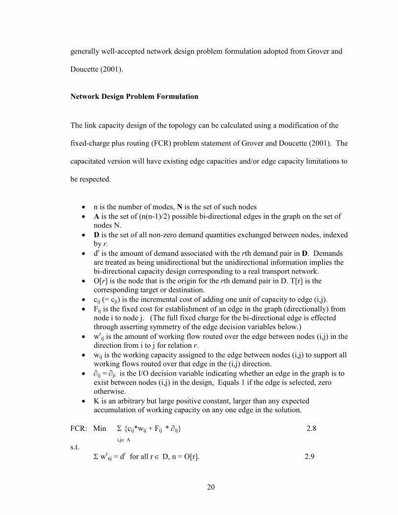
The link capacity design of the topology can be calculated using a modification of the

fixed-charge plus routing (FCR) problem statement of Grover and Doucette (2001). The

capacitated version will have existing edge capacities and/or edge capacity limitations to

be respected.

• n is the number of modes, N is the set of such nodes • A is the set of (n(n-1)/2) possible bi-directional edges in the graph on the set of

nodes N. • D is the set of all non-zero demand quantities exchanged between nodes, indexed

by r. • dr is the amount of demand associated with the rth demand pair in D. Demands

are treated as being unidirectional but the unidirectional information implies the bi-directional capacity design corresponding to a real transport network.

• O[r] is the node that is the origin for the rth demand pair in D. T[r] is the corresponding target or destination.

• cij (= cji) is the incremental cost of adding one unit of capacity to edge (i,j). • Fij is the fixed cost for establishment of an edge in the graph (directionally) from

node i to node j. (The full fixed charge for the bi-directional edge is effected through asserting symmetry of the edge decision variables below.)

• wrij is the amount of working flow routed over the edge between nodes (i,j) in the

direction from i to j for relation r.• wij is the working capacity assigned to the edge between nodes (i,j) to support all

working flows routed over that edge in the (i,j) direction. • ∂ij = ∂ji is the I/O decision variable indicating whether an edge in the graph is to

exist between nodes (i,j) in the design, Equals 1 if the edge is selected, zero otherwise.

• K is an arbitrary but large positive constant, larger than any expected accumulation of working capacity on any one edge in the solution.

FCR: Min Σ {cij*wij + Fij * ∂ij} 2.8

i,j∈ As.t.

Σ wrnj = dr for all r ∈ D, n = O[r]. 2.9

21

nj∈ A

Σ wrjn = dr for all r ∈ D, n = T[r]. 2.10

jn∈ A

Σ wrin - Σ wr

nj = 0 for all r ∈ D, for all n ∉ {O([r],T[r])} 2.11 in∈ A nj∈ A

wij = Σ wrij for all i,j∈ A 2.12

wij <= K * ∂ij, ∂ij = ∂ji, ∂ij ∈ {0,1}, wij integer for all ij ∈ A. 2.13

2.8 objective statement, minimize cost of network while routing all traffic demands between node pairs.

2.9 2.10 and 2.11 are the flow balance constraints of the node-arc transportation problem. They assert that the total source flow equals the demand and that the total sink flow also equals the demand, and that no net sourcing or sinking of flow for the given O-D pair occurs at any other node (i.e., “trans-shipment”).

2.12 Definition of required edge capacity in terms of the simultaneous flows over the edge 2.13 set of constraints that establish the boundary on wij, the 0,1 values for ∂ij, and the integer constraint on the working capacity of the link.

III. Multi-level or Hierarchical network design

Most physical networks today are a mesh of nodes and links with logical topologies

overlaid on the mesh. Each logical overlay operates as a separate network independent of

other networks. Increasingly the need is to merge these distinct networks into one unit

operating as one network with several layers. This section of this paper will review some

of the relevant literature relating to combining topologies and using logical topology

design, LTD, to overlay logical topologies on physical topologies to expand network

functionality as well as the general problem of network link design. There has been a

wide variety of research published covering applying optimization techniques to multi-

22

level telecommunication networks. Some of the classic contributions in the field are

Cahn (1998), Balakrishnan et al (1995), Kershenbaum (1993), Chang and Gavish (1993),

and Gavish (1991).

The design process to define the optimal topology or near optimal topology for a network

should take into account the diverse nature of the traffic carried. Each traffic type has its

own special characteristics such as tolerance for delay, restoration needs and tolerance for

packet loss. The legacy optical core networks for the most part are ring topologies that

are optimized to give the best performance for voice traffic. While rings provide fast

restoration needed to support circuit switched voice traffic, mesh networks provide

greater efficiency in the use of network resources and can be more economical to deploy.

With the advent of optical switches and DWDM, mesh topologies were optimally

designed to carry data traffic.

An early approach to this concept was to design a hierarchical network with two physical

topologies. Lee, Ro, and Tcha (1993) present a two-level hierarchical network structure

with the upper level as a hub-ring and the lower level access network with star-type

connections. By partitioning the whole problem into two easy problems, a dual-base

approach can be used to formulate the design problem into a mixed 0-1 integer-

programming model. A heuristic procedure is used on the dual-based lower-bounding

solution to construct a primal feasible solution from the dual procedure.

Brown et al (1994) presented a comparison of two architectures, mesh/ring, and mesh/arc

for survivable self-healing transport networks. In mesh/arc networks, the core consisted

entirely of mesh connections and the access portion of the network is either incomplete

23

rings or “arcs” of add-drop multiplexers. Mesh/ring networks are mesh core networks

with ring topologies for access. They presented the case that mesh/arc architecture

topologies could recover from failure relatively quickly and were cheaper to deploy than

mesh/rings. Mesh/arc were also more flexible in reacting to traffic demand changes.

Chang and Gavish (1993) presented a formulation using a primal heuristic and a dual-

based lower-bounding procedure for subproblems of the larger overall problem.

Lagrangian relaxation was used to decompose the problem into two independent

optimization problems; a continuous routing, capacity expansion problem, and a minimal

spanning tree problem. Combining these subproblems with a lower bound for the main

problem, a branch-and-bound procedure to do a global search using a heuristic was

described to solve the problem.

Yoon, Baek, and Tcha (1998) presented a design methodology for a distributed fiber

transport network using hubbing technology. This formulation of the complex network

design problem redefined commodity flows using a dual-based heuristic that yielded

near-optimal designs. Mukherjee, et al (1996) presented the concept of an arbitrary

virtual topology embedded on a given physical fiber network to exploit the advantages of

wavelength multiplexers and optical switches in wavelength routing. They introduced

the concept of “all-optical lightpaths” that are set up to carry packets as far as possible

over the stream of wavelengths in the optical domain only converting back to electronic

domain when necessary. Their approach was to formulate an optimization problem that

optimally selected a virtual topology subject to transceiver and wavelength constraints

using two functions, first to minimize the network average packet delay and second, to

24

maximize the scale factor by which the traffic matrix can be scaled up. Since these types

of problems quickly become NP-hard they used a heuristic approach to solve the

problem. It was an iterative approach that combined simulated annealing algorithms to

search for a good topology and flow deviation approaches to optimally route the traffic

on the virtual topology.

Guo, Acampora, and Zhang (1997) described a hyper-cluster solution for scalable and

reconfigurable wide-area lightwave network architecture. A hyper-cluster approach uses

a logical hierarchy for addressing but insures that all nodes have the same number of

transceivers. Hyper-clusters are a cluster of regular graphs with a clustering structure that

follows traffic distribution. Prathombutr and Park (2002), as a way to design a multi-

layer optical network, using logical topologies presented clustering to create subdivisions.

The logical topology, a set of lightpaths formed to serve traffic demands, was created by

analyzing traffic demand and the physical topology to classify the nodes into either

Optical layer or Electrical layer. The clustering method uses the multivariate analysis to

cluster the data by a combination of characteristics of the network nodes. These

characteristics can include cost of equipment, location, policy, or other factors deemed

important for the design.

Tran and Beling (1998) presented a heuristic approach to design the topology of a two-

tiered network by integrating access area and backbone design problems into a single

mathematical program. Since this type of problem is quite difficult to solve, usually the

problem is subdivided. While enhancing the solvability of the problem, subdividing can

25

produce inferior results. Using simple probability models on link costs also simplifies the

procedure.

Banerjee and Mukherjee (2000) defined a solution to the LTD using an exact integer

linear programming formulation that minimized the average packet hop distance. This

approach was equivalent to maximizing the total network throughput under balanced

flows using lightpaths. Balancing resource tradeoffs between transceivers and switch

sizes can create a well-balanced network with good utilization rates. Additionally, their

problem formulation provided a reconfiguration methodology to allow the virtual

topology to adapt to changing traffic conditions.

LTD defines logical topologies that will minimize congestion (Krishnaswamy and

Sivarajan 2001). The authors present a general linear formulation that considered routing

traffic demands by routing and assigning wavelengths to lightpaths as a combined

optimization problem. Their solution worked well for small examples but for large

networks, the integer constraints were relaxed and a lower bound on congestion was

established. Another approach to LTD presented by Lee et al (2000) used a multi-

commodity flow approach to define the problem. They created a general cost function

that covered all system components and presented two solutions, one based on integer

programming and the other on heuristics developed to solve this problem. The integer-

programming approach yielded the network configuration with the minimum

implementation cost but the problem was of immense size. The heuristic based on a

minimum variance algorithm performed considerably better than other presently used

algorithms such as shortest path.

26

Sen, Bandyopadhyay, and Sinha (2001) presented an alternative method for examining

the structure of the LTD problem. This work examined the problem from a graph theory

perspective. While previous graph theory work presented the overlay as a regular

structure such as hypercube, de Bruijn graph, Kautz graph, and Cayley graph, this paper

proposed a generalized multimesh (GM), a semi regular structure. By developing a new

metric, flow numbers can be used to evaluate topologies. Flow number is the minimum

threshold capacity on the links in that network that is able to sustain a traffic flow. Much

work has been done in the graph theory examining how to connect or create overlays but

very little has been applied to telecommunication network design.

LTD problems can focus on different parameters such as reliability. Arakawa, Katou,

and Murata (2003) present a new concept called “Quality of Reliability (QoR), a

realization of QoS with respect to the reliability needed in a WDM network. QoR was

defined in terms of the recovery time from when a failure occurs to when traffic on the

affected primary lightpath is switched to the backup lightpath.” A heuristic algorithm

was proposed that designed a logical topology that satisfies the QoR requirement set forth

for every node pair. Their objective was to minimize the number of wavelengths needed

in the logical topology to carry the traffic required QoR. Initial results from this

approach indicate that 25% fewer wavelengths are needed than with other algorithms.

Grover and Doucette (2002) developed a methodology using a meta-mesh chain of

subnetworks to increase the capacity efficiency on spare facility graphs. A loop-back-

type space capacity is provided only for the working demands that begin or end in a chain

and not for the entire flow that crosses a chain. The express flows (those that begin or

27

end elsewhere) are entirely mesh-protected within the meta-mesh graph that is of higher

average degree of nodal connectivity. This approach creates a new class of restoration

that is intermediate between span and path restoration with most of the efficiency of path

restoration and nearing the localized nature and speed of span restoration.

Cruz, MacGregor Smith, and Mateus (1999) developed a solution to solve to optimality

the uncapacitated fixed-charge network flow problem (FCN) using a Lagrangian

relaxation to define boundaries. Their approach was to develop a solution to the multi-

level network optimization (MLNO) problem that integrates into the same model

location, topology and dimensioning of a network. While the initial application of this

work was for the design of electrical power systems, interconnecting powerstations and

load centers of a national power grid, the multi-characteristic nature of a

telecommunications network is another area that this approach might prove powerful.

Dahl, Martin, and Stoer (1998) presented a routing solution through virtual paths in a

layered network. Their solution was developed using an integer linear programming

model where 0-1 variables represented different paths. A cutting plane approach

produced reasonable results for solving real world pipe selection and routing paths.

Peusch, Kuri, and Gagnaire (2002) proposed an approach to the multi-commodity flow

problem used to formulate the LTD problem and the lightpath routing (LR) problem

using mixed integer linear programming techniques. By tackling the two problems, LTD

and LR, with separate models the problem becomes realistically solvable. By

modularizing the approach, different combinations of the optimization models and the

objective functions are developed.

28

Grosso et al (2001) used Tabu search optimization meta-heuristics to develop a logical

topology over a WDM wavelength routed network. They formulated the LTD problem

for traffic affected by a degree of uncertainty using a stochastic description of the traffic

pattern, an existing topology, and a multi-hop routing strategy. Their results suggest that

local search techniques such as Tabu are promising and worthy of further investigation.

Shyur and Wen (2001) also presented a methodology for solving a similar problem of

virtual paths in an ATM system. Their approach seemed to show better performance than

the existing random path algorithm especially as the problem size grows larger.

Marsan et al (2002) presented a mixed integer linear programming, MILP, formulization

of the optimal logical topology, LTD, with multicast traffic under deterministic and

stochastic traffic patterns. Using greedy and metaheuristic (Tabu) algorithms, an optimal

design to the NP-hard problem was found. Lower bounds and numerical results showed

that their proposed metaheuristic Tabu-based formulation outperformed other greedy

approaches. Extending the problem to handle changing traffic patterns their proposed

methodology found no degradation in the solution.

III. Multi-level (or Hierarchical) Network Design Problem

The multi-level or hierarchical network optimization (MLNO) problem is formulated

using a similar approach to that of the basic network design problem but uses different

cost functions for each level in the design. Cruz, MacGregor Smith, and Mateus (1999)

present the MLNO as follows:

L = {set of all levels in design l = 1,2,…m} Rl = {set of lth level candidate supply nodes}

c lij = non-negative per unit cost for the lth level flow on arc (i,j) x lij = lth level flow through arc (i,j)

29

f lij = non-negative fixed cost for using arc (i,j) to support lth level flow

y lij = Boolean variable which assumes the value 1 or 0 depending on whether or not the arc (i,j) is being used to support lth level flow

fi = non-negative allocation for the lth level candidate supply node i zi = Boolean variable which is set to 1 or 0 depending on whether or

not the node i is being selected to provide lth level flow

Min Σ [ Σ (cijl xij

l + fijlyij

l) + Σ fizi ] 2.14 l∈L (i,j)∈A i∈Rl

with similar constraints to those listed in section II Network Topology Design.

Summary

The multi-level network design has received much attention so that combining designs

can improve the performance of the network. One of the basic premises is that there will

be different costs for each level of the network. This study will use the same cost

function for each link regardless whether it is functioning as a backbone link connecting

concentrators (backbone nodes) or access link connecting terminals (end nodes) to

concentrators. Using the same cost function for each level, the multi-level concept

therefore is not a part of this problem.

IV. Multi-period Design Approaches that include Growth

Adding the multi-period component to the problem enlarges the problem of network

topology and capacity design to include the concept of expansion. Most approaches are

iterative techniques that compare the formulation results for each planning phase to

determine the optimal solution by either sequential single period formulations or dynamic

formulations. Sequential single period formulations require the output of period t be the

input of the t+1 period.

30

Chang and Gavish (1993) present an LP formulation of the design and capacity

expansion problem with a family of heuristics and a dual-based lower bounding

procedure using Lagrangian relation and a global search strategy. Garcia, Mahey, and

LeBlanc (1998) formulated a model with discrete characteristics that have changing

monthly (but not minute-by-minute) point-to-point traffic requirements and budget

constraints. This formulation does not include congestion and capacity considerations. It

uses a generic self-calibrating local improvement template algorithm purported to

improve the performance and flexibility of classical approaches that solve the design of

the network with changing traffic requirements.

Pickavet and Demeester (1999) introduced a mathematical model of the multi-period

reliable network-planning (MPRNP) problem to compare single-period planning verses

multi-period planning. They used two different techniques, a sequential single-period

approach, and an integrated multi-period approach. The multi-period approach puts more

emphasis on scheduling the right investments at the right time. Extensive simulations on

a wide range of problem instances showed that the integrated multi-period approach leads

to a cost savings (average 4.4%) on the problem investments over the more traditional

sequential single-period planning approach. The relative differences were rather small

but when comparing the three cost model approaches the choice of algorithmic model

used was more important than the cost model. No clear influence of network size,

relative growth demand over planning horizon, or presence of an initial network was

detected.

31

Ouorou, Luna, and Mahey (2001) looked at the multicommodity network expansion

under changing demands problem. They applied a generalized decomposition method to

a mixed integer nonlinear formulation of the integrated problem of network design and

decomposition. Their two-step procedure incorporates a master program level that

proposed to expand capacities on some arcs and a convex cost multicommodity flow

subproblem including price sensitive demands. This topology-tuning approach combines

the allocation of bandwidth with the routing of traffic to develop an effective solution.

IV. Multi-period Design Problem Modified after Chang and Gavish (1993) the following is a formulation of the network

design problem with multiple periods.

Definitions: A = set of all links ij.cij = cost function for each link from i to j per capacity unit. wij = capacity needed on link i to j. T = { set of planning periods, t = 1, 2,…n}. Min Σ Σ {cij

t*wijt } 2.15

t∈T i,j∈ A

subject to:

similar constraints as above plus

cijt - cij

t-1 >= 0, for all i,j ∈ A and for all t ∈ T .

32

Summary

A multi-period design problem allows the optimization study to examine changes in

multiple periods and define by time period, monetary investments or growth. Pickavet

and Demeester, 1999, showed that the only important factor between sequential single

period investment and multiperiod dynamic was the timing of investments. Since this

study is examining the impact of nodal distribution strategies the sequential single period

process will be used because in this study there will be no real time associated with the

growth periods only the amount of growth.

Efficient or Production Frontier

Using the Efficient Frontier, a concept borrowed from finance, agriculture economics,

and operations research literature, (Markowitz, 1959 and Farrell, 1957) the design

process creates a set of designs that are efficient combination of chosen parameters. The

efficient frontier represents a suite of efficient combinations of nodes and links for the

problem and the cost of any design can be related to the frontier thereby essentially

measuring the efficiency of that design. A brief discussion of the Efficient Frontier

concept will be presented but interested readers are referred to Fare et.al (1994) and

Copeland et.al (2005) for more comprehensive discussions.

By developing a set of designs by doing sensitivity analyses, the designer creates an

envelope of cost functions. The lower boundary of this envelope is the efficient frontier

or suite of “best” designs as far as the parameters used for the optimization. The

efficiency of any design is the relationship of the final cost of a design to the frontier.

Evaluating the distance any point is from the efficient frontier gives a measure of the

33

efficiency of the design as related to the parameters used in the optimization. The closer

the design cost to the efficient frontier the more efficient the design. By understanding

the impact of design changes to the final cost of the network, well-informed design

changes can be implemented with regard to final or long term cost.

Traffic models and projections

There are several previously published approaches to developing the traffic matrix (Cahn

1998). The first method is to assume an equal level of traffic between all node pairs.

While this is the simplest approach, it is the least realistic. It is often used in the initial

proof-of-concept testing of the methodology as well as exploring the effects of other

parameters outside of traffic modeling. Second, population density of a city is used as

the size factor for determining the type and amount of traffic between city pairs. Larger

population centers would exchange more traffic than smaller population centers and may

grow at different rates. This approach is more realistic but is more complex.

For the most part, network-planning models in use today were designed for voice traffic

on the plain old telephone system networks (POTS). The growing impact of data traffic

associated with the explosive growth of the Internet and multimedia applications such as

KaZaA that deliver MP3 music files has changed the focus of network traffic models.

Some reports estimate that more than 60% of traffic carried on networks today is data and

the growth of data related traffic is not expected to slow. While the amount of data traffic

carried on networks is growing, the main revenue source for network carriers is still voice

traffic (Maesschalck et al 2003). Thus, traffic models that emulate connection oriented

circuit switched traffic still dominate the network-planning field.

34

New traffic models are needed to accurately emulate the changing nature of today’s

traffic but also carefully adjust for voice traffic, the major source of revenue for carriers.

Dwivedi and Wagner (2000) presented a model that differentiated between three traffic

types: voice traffic, transaction data traffic (mainly business generated modem and IP

traffic), and Internet traffic (IP traffic not related to business environment, mainly

downloading of WWW pages). This traffic model was modified and used by

Maesschalck et al (2003) for a topology comparison of the Pan-European carrier

networks. Generally, network planners when developing new traffic models either use

historical trends based on internal data or on various models that relate population

density/size for a given area and distance between city pairs as predictors of volumes of

traffic (Cahn 1998). These models usually make growth assumptions based on the

population census data for a given geographic area that work very well for predicting

voice traffic change but do not differentiate traffic types. In today’s Internet environment

the basis has changed and new models are needed. Dwivedi and Wagner (2000)

presented a traffic analysis with a generalization of Internet traffic in1999 captured by the

following: “for voice traffic assume 14 minutes of long-distance traffic person per day, 5

minutes of transaction modem use per non-production employee per day, and 25 minutes

of continuous modem access to the internet per host per day” (Dwivedi and Wagner

2000). Using this data to develop proportionality constraints, the total traffic pattern is

best modeled using the following equation:

Voice traffic (i, j) = Kv* Pi * Pj / Dij

Transaction data traffic (i,j) = KT * Ei* Ej / √Dij

35

Internet traffic (i,j) = KI * Hi * Hj

The traffic between cities i and j depends on the total population Pi, the non-production

business employees Ei, and the number of Internet host Hi, in each city as well as the

distance Dij between the two cities of interest. Growth rates based on US census data

were calculated and average growth rate for each traffic type was predicted. Voice traffic

was extrapolated to grow at 8% per year, transaction data traffic at 34% per year and

Internet traffic at 157% per year. This analysis was done during 1998-1999, the peak of

the e-commerce dotcom boom times, and estimations seemed good for the times. Since

then, published reports have indicated that the number of Internet users has grown at

about 40% per year (Maesschalck et al 2003). Other recent reports have indicated that

Internet traffic is expected to double every year (Legard 2003). Even with the

uncertainty in Internet traffic growth, breaking traffic-growth projections into individual

components is certainly a valid approach, although more complex than using one type of

traffic.

Summary

In summary, the scope and depth of the efforts to define methods that develop the optimal

or near optimal network design are significant. Much work has been done to develop

techniques for network design to define optimal or near optimal results but still there is

no clear best method or solution technique. Logical overlays or virtual topologies and

multiple-growth periods have had some attention but no studies were found that

compared nodal distribution strategies. The development of traffic models is still very

subjective and much work needs to be done. A traffic matrix using population-based

36

values is the most commonly used process most likely due to the ease of data access,

usually national population surveys. The research effort presented in this paper will

focus the impact of nodal placement strategy upon long term cost effectiveness of a new

service overlay on a legacy network topology. The next chapter will discuss the

mathematical model used in this study.

37

CHAPTER 3 MATHEMATICAL MODEL

This study set out to answer three questions. First, what is the most cost effective switch

distribution strategy for a new service overlay on an existing network for long term

growth; overlay switches distributed over many legacy nodes, or overlay switches

distributed over one or a very few legacy nodes? Second, what does the efficient frontier

of overlay switch designs and costs look like as overlay network designs deviate from the

best? And lastly, are there heuristics that can be defined to help point the way towards the

least cost design? This section will present and analyze the cost model used to answer

these three questions.

Mathematical Model

For this study the cost for each growth period of the new service overlay is defined by the

following equation (Equation 3.1)

Overlay System Cost = Overlay Switch Cost + Overlay Link Cost. 3.1

The overlay switch cost consists of two parts; the cost for the switch chassis and the cost

for each of the ports or connections needed to accommodate the traffic flow through the

overlay switches. Overlay link cost is related to the length of the links and the capacity

of the links used in the overlay.

38

Overlay Switch Cost = Overlay Chassis Cost + Overlay Port Cost

An overlay network consists of backbone nodes and access nodes. An access node will

not require an overlay switch, while a backbone node will require an overlay switch.

Overlay backbone switches will have a minimum of two overlay logical connections, and

overlay access nodes will attach to a backbone switch via a single logical connection

utilizing assets of the underlying legacy network.

Overlay Chassis Cost

The chassis cost for each overlay backbone node is captured by a function that is

dependent upon the number of connections or flows that must move through the switch.

As the number of traffic flows increases beyond a certain point, a larger more expensive

switch may be required. The actual cost function of the chassis increases in a step-like

manner based on the number of connections needed (Figure 1). An alternative method

would be to model the chassis cost with a smooth function that shows a similar reduction

in unit cost with growth in the size of the switch chassis (Figure 1). There are some

economies of scale that can be achieved with larger switches. Usually there will be a

reduction in cost per unit connection over smaller switches.

39

Figure 1 Cost function for the overlay switch chassis. While the actual function is step-like, it can be modeled with a function that shows the reduction in unit cost with growth in size of the switch chassis. This is a log-normal plot.

Individual Overlay Chassis Cost

The experimental method discussed in chapter 4 uses the actual step function to model

chassis costs. The approximation of the step function is used in this chapter, as it is

easier to visualize changes in switch costs as traffic flow increases with the smooth

approximation function. The individual overlay switch chassis cost is defined by the

following equation (Equation 3.2).

Individual Overlay Chassis Cost = xi (C1 + K1 * (nodei_traffic)α), 3.2

40

xi = binary constant, (0 or 1) indicating whether or not an overlay switch is located at

node i.

nodei_traffic = the amount of traffic flow that will move through the node i. Also called

the number of connections needed at a switch.

C1 = initial cost of chassis

K1 = arbitrary unit cost of a chassis

α = Exponential factor that modifies the impact of traffic flow upon the size of the

switch chassis. α < 1. The closer α is to 1, the closer the function is to linear. A value

of α less than 1 allows economies of scale to be captured. α = 1 in this study.

Total Overlay Chassis Cost

The total overlay chassis cost for the network is modeled by summing the chassis costs

over the entire network overlay (Equation 3.3).

n

Total Overlay Chassis Cost = ∑ [xi (C1 + K1* nodei_trafficα)] 3.3 i=1

N = set of nodes in the network overlay, {1, …, n}.

Overlay Port Costs

Port/connection costs are the second part of the overlay switch cost. For each connection

that is needed to and from an overlay switch there is a per port/connection cost.

Generally there is a flat per port or connection cost as modeled by Figure 2. Although,

economy of scale effects can be seen when purchasing large volumes, so β (as defined

below) can be < 1.

41

Figure 2 Connection or port cost model. This is modeled by a simple linear cost per unit function. Although with different cost functions β could be less than 1 reflecting a cost structure that allows for economies of scale.

Individual Overlay Switch Port Costs

Port cost for an individual overlay switch is modeled by the following equation (Equation

3.4).

Port Costi = K2 * (nodei_traffic)β 3.4

K2 = an arbitrary unit cost assigned to each connection.

β = an exponential factor that will describe the shape of the curve, β < 1. For this study

β = 1 but with different cost functions β could be less than 1 reflecting economies of

scale.

42

Total Overlay Port Cost

Total port cost is found by summing the individual overlay switch port costs together

over the entire overlay network design (Equation 3.5).

n n

Total Port Cost = ∑ xi Port Costi = K2∑ xi (nodei_traffic) β 3.5 i=1 i=1

Overlay Link Costs

Overlay link costs are a function related to the length of the link and the capacity or size

of link used in the overlay to deliver the traffic flow (Figure 3).

43

Figure 3 Overlay Link Cost - Cost for overlay link cost is based on both the amount of bandwidth or capacity needed and the length of the link. The shape of the cost function will depend upon the relationship between distance and bandwidth cost. The relative relationship between bandwidth and distance will determine the shape of the curve. For this figure the cost of distance and the cost of bandwidth are approximately the same.

Individual Overlay Link Costs

Overlay link costs for an individual link are modeled by the following equation (Equation

3.6).

Overlay Link Costs = KL * Capacityijχ * Distanceij

δ 3.6

KL = an arbitrary unit cost factor

Capacityij = link capacity from node i to node j

44

Distanceij = route miles from node i to node j

χ and δ; exponential factor for traffic and distance respectively. For this study χ and δ = 1

but other cost models could have these values less than one. For instance, some Frame

Relay service providers do not price connectivity in terms of distance so δ could be equal

to zero. Other cost models with χ < 1 could show economies of scale related to capacity.

Total Overlay Link Costs

Total overlay link costs for overlay designs are modeled by summing the cost for each

over the entire overlay network (Equation 3.7).

n n

Total Overlay Link Costs = KL * ∑ ∑ (Capacityij)χ * (Distanceij)δ 3.7

i=1 j=1

Total Cost of a New Service Overlay on a Legacy Network

The total cost of a new service overlay would be the sum of the above stated equations,

(Equations 3.3, 3.5, and 3.7) represented by Equation 3.8.

Total Overlay System Cost = total Overlay Chassis Cost + total Overlay Port Cost + total Overlay Link Cost

n

= ∑ [xi (C1 + K1 * (nodei_traffic)α)] i=1

n

+ K2 ∑ xi (nodei_traffic)βi=1

n n

+ KL * ∑ ∑ (trafficij)χ * (distanceij)δ 3.8 i=1 j=1

i = indicates which node from the set N= {1,2,…,n} where n is the total number of nodes

in the overlay design. The set of i = the set of j.

45

To understand how to minimize the total cost of the overlay network as defined in

Equation 3.8 above, the components of overlay switch and overlay link are best examined

separately. Minimizing overlay switch costs, including both chassis and port costs,

requires that the number of overlay switches be minimized as well as the sum of the

traffic flows per node be minimized so that at each node there will be the fewest ports

and smallest chassis. To accomplish the fewest number of ports, generally, each traffic

flow should be routed through the minimal number of overlay switches. Each flow

should be moved along the most direct path, i.e. the path with the fewest hops in the

overlay network. Minimizing the number of hops would be easiest in overlay designs

with high connectivity. Designs with minimal number of paths, such as a ring topology,

would force all traffic flows to follow the same paths thereby creating the need for larger

switches that handle more traffic. Note though, that if α and/or β < 1, economies of scale

may make it cheaper to route certain traffic flows through a larger number of switches.

To minimize overlay link costs, traffic flows should generally be routed along the

shortest path. In this study where the full impact of the cost of distance is a part of the

cost model, i.e. δ = 1, the shortest path is least costly. If χ or δ are < 1, link costs might

very well be minimized by aggregating lightly used direct links onto two or more indirect

links that are more heavily loaded. Examining the impact of link utilization, when χ or δ

are < 1, upon the question of overlay switch distribution was not considered in the case

studies presented in following chapters. This is a subject for future research.

Minimizing overlay switch costs and overlay links costs can be but are not necessarily

mutually compatible. The shortest path is not always the one with the fewest hops.

46

Additionally, whether switch or link costs will dominate the process depends also upon

the relative relationship of the values of the unit cost functions. The next section of this

chapter will examine this aspect.

Cost Relationships

The relative relationship between the unit cost of overlay links and the unit cost of

overlay switches will tend to determine which factor in the total cost equation (Equation

3.8) will have the most impact. This discussion focuses entirely on the overlay cost

functions and not the legacy network. Figures 4, 5, and 6 show the impact of varying the

relationship between the unit overlay link costs, KL, and unit overlay switch costs, KS.

KS is a generalized sum of K1 and K2 defined above as the unit cost of overlay switch

ports and overlay switch chassis. When the unit cost of an overlay link, KL, is

significantly greater than the unit cost of an overlay switch, KS, or KL >> KS, the driving

factor towards the total cost will tend to be the cost of links (Figure 4).

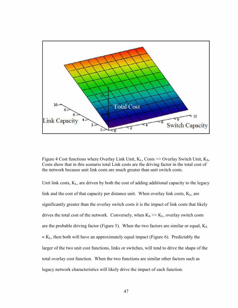
47

Figure 4 Cost functions where Overlay Link Unit, KL, Costs >> Overlay Switch Unit, KS,Costs show that in this scenario total Link costs are the driving factor in the total cost of the network because unit link costs are much greater than unit switch costs.

Unit link costs, KL, are driven by both the cost of adding additional capacity to the legacy

link and the cost of that capacity per distance unit. When overlay link costs, KL, are

significantly greater than the overlay switch costs it is the impact of link costs that likely

drives the total cost of the network. Conversely, when KS >> KL, overlay switch costs

are the probable driving factor (Figure 5). When the two factors are similar or equal, KS

≈ KL, then both will have an approximately equal impact (Figure 6). Predictably the

larger of the two unit cost functions, links or switches, will tend to drive the shape of the

total overlay cost function. When the two functions are similar other factors such as

legacy network characteristics will likely drive the impact of each function.

48

Figure 5 Overlay Link Unit KL costs << Overlay Switch Unit KS costs. In this scenario

switch/port cost is the driving factor.

49

Figure 6 Overlay Link Unit KL Cost ≈ Overlay Switch Unit KS Cost. When each factor, link and switch costs are about equal, each will have about the same impact to the total cost function.

This discussion while relatively straightforward shows the impact on the final overlay

total cost of changing the relative relationship of the parts of the total function. The

previous discussion is specific to α, β, χ and δ = 1. It becomes more complicated when

economies of scale come into play and α, β, χ and δ ≠ 1. In the telecommunications

industry, there are many approaches to determining cost functions and the impact of each

factor on the total function. Future research could vary the values of α, β, χ, and δ and

examine the impact of economies of scale.

Overlay link unit costs can dominate when constructing a brand new overlay network

requires laying cable, building all the physical support hardware for the cable links, and

50

all of the associated installation costs. When a network operator decides to put additional

functionality on its legacy network, additional link unit costs might be limited to those

associated with reassigning link capacity that could be less than the cost of the overlay

switches and other switch related costs. Another example of a cost function where the

impact of link costs might be very low would be a Frame Relay revenue function. In this

case, the user might pay for just the bandwidth committed and not the distance of the

links used. While simplified, the examples presented above do represent real world cost

functions.

The purpose of this research was to investigate the impact of the number and location of

overlay switches on the total overlay cost function. In some overlay designs, the cost of

adding link capacity would dominate the cost function, while in others the switch cost

function could dominate. The North American, NSFNet and Pan-European test cases

examined in this study used overlay switch and overlay link costs of similar relative

value, though KS was greater than KL. For this study and α, β, χ, and δ, = 1. Other

relationships of α, β, χ, δ, and K would be the subject of future research.

Network Design Heuristics For Choosing Locations Of New Service Overlay Switches On A Legacy Topology

The following discussion outlines three design heuristics that when applied to the

network design process can help lower the total cost of a new service overlay on an

existing legacy network. Given that this is an intractable NP-hard problem the heuristics

as applied may have a limited impact but should help guide towards a low solution. The

basic concepts of the three heuristics, connectivity, location and traffic volume, are well-

51

known network design concepts discussed in many references including Cahn, 1998 and

Drezner and Hamacher 2002. This research applies these concepts to designing a new

service overlay on a legacy topology.

The cost model used to develop the application of these heuristics was Equation 3.8

where α, β, χ and δ = 1. The heuristics stated below should be applicable with other

choices of α, β, χ and δ, but to a varying extent and are the subject of future research.

The three heuristics are as follows; locate overlay switches at nodes in a centralized

location of the legacy network as opposed to the periphery, locate overlay switches at

legacy node locations with high connectivity, and lastly, locate overlay switches at legacy

nodes with high traffic flow demand. While each heuristic describes a different concept

these ideas tend to work in concert and the impact of each will not always individually be

definable. Each heuristic will be discussed individually in the following part of this

chapter.

Heuristic 1 - Locate overlay switches at nodes in a centralized location

of the legacy network

Locating overlay switches at centralized locations within the legacy topology can help

reduce total link costs because traffic flow paths should tend to be shorter. Backhaul

distances of traffic flows from source node to the nearest overlay switch to reach the

overlay backbone will be shorter when overlay switches are located at a central location.

Reducing total link cost is important when link cost dominates the total cost function and

when the full impact of link distance is a part of the total link cost equation, i.e. Equation

52

3.7, δ = 1. When distance is less important to the total cost, i.e. δ < 1, minimizing link

costs by keeping total link distance at a minimum will have less of an impact upon total

cost and therefore the impact of this heuristic will be less. As δ decreases to 0, total link

distance will have less and less of an impact on the total cost of the overlay and the

centralized core location of an overlay switch will be less important. Knowing the form

of the cost function prior to designing the overlay will be important for minimizing costs.

Heuristic 2 - Locate overlay switches at legacy node locations with high

connectivity

Choosing to locate overlay switches at legacy node locations with high connectivity can

help minimize link costs as well as possibly switch costs. With more link connections

available, traffic flows will have more routing options creating a higher probability of

each traffic flow being routed via the shortest route. This will reduce link costs because

route path distances will be less. Choosing switch locations with higher connectivity on

the legacy topology can reduce backhaul distance costs because traffic flows can likely

be routed on a more direct path from access nodes to the nearest overlay switch. Switch

costs can be impacted because with more path choices traffic flows can potentially be

routed through fewer switches creating the need for fewer total connections and possibly

smaller switch chassis.

53

Heuristic 3 - Locate overlay switches at legacy nodes with high traffic

flow demands

Locating overlay switches at legacy nodes with high traffic flow demand should help

reduce total overlay costs by reducing link costs. If a large amount of traffic flow is

generated at a node site without an overlay switch, traffic flow path distances will be

increased because the entire traffic flow will have to be carried to a single overlay switch

before entering the overlay backbone. As a result, some of that traffic will likely initially

travel in the wrong direction resulting in large traffic flows being inefficiently routed,

potentially increasing the cost for links. Hence, placing switches at nodes with high

traffic demands will offer the potential to reduce the distance a large amount of traffic

might have to be backhauled thereby reducing link costs.

Switch costs might also be reduced. For example, suppose a node Edge1 has U units of

traffic, and an overlay switch is not placed there. The node is then an edge node and will

have a single overlay connection, moving U units of traffic, to an overlay backbone

switch at node Backbone1. This backbone switch will now have to handle U – U2 units

of traffic coming in, and U – U2 units of traffic going out, that it would otherwise not

touch, U2 being traffic from node Edge1 that would normally hit the backbone switch at

node Backbone1 even if the node Edge1 had a backbone switch. Money is saved as a

switch with capacity U at the edge node is not needed but the capacity of the backbone

overlay switch must be increased by 2(U – U2) units. Depending on the values of U and

U2, and the cost function, this may or may not result in switch cost savings.

54

Backhaul of Traffic Flow

Backhaul is the movement of traffic flow from an access node that is not on the overlay

backbone to an overlay switch on the backbone. Figure 7 illustrates the backhaul

concept. Overlay backbone switches are located at nodes 1 and 3 but not at node 2.

Node 2 is an access node whose traffic flow needs to be hauled to a switch on the overlay

backbone. Traffic flow that must move from node 2 to node 1 will first be carried to an

overlay switch, in this case to the switch at node 3 and then on the overlay backbone via

the logical link 1-3 to the overlay switch nearest its destination. In this example, logical

link 1-3 traverses through node 2 but utilizes resources of the underlying network. Note

in Figure 7 traffic flow from node 1 to node 2 would travel over the legacy network link

between nodes 2 and 3 twice, once as it is moved from overlay switch 1 to overlay switch

3, and again as it is hauled back to access node 2. Backhaul of traffic flows increases link

costs because inefficient routing (going out and back on the legacy network link between

nodes 2 and 3) necessitates the use of larger capacity links from the underlying legacy

network. As far as the overlay switches at nodes 1 and 3 are concerned they have a direct

connection with each other and are likely not aware that traffic actually passes though

node 2. Were an overlay backbone switch also located at node 2, switch costs would

increase due to the addition of this switch, but link costs would decrease as traffic flow

from nodes 1 and 2 could travel directly between the two locations and not via the route

2-to-3-to-1.

55

Figure 7 Backhaul of traffic flow to an overlay switch. For this example, a logical backbone link between nodes 1 and 3 is created because the overlay backbone does not have a switch at node 2. The traffic flow to and from node 2 will be carried to the nearest switch, in this case at node 3. The flow to node 1 would be carried along link 2-3 first to node 3 and then back across logical link 1-3 to node 1. It will be carried on the legacy link between nodes 2 & 3 twice

Examples of Heuristics

A series of simplified examples illustrating the impact of the heuristics are described in

the following section. Figure 8 illustrates an example of the impact of placing an overlay

switch in a centralized location of the legacy network versus a perimeter location as well

as at a node with high connectivity. A 5-node legacy network with one central node is

presented to illustrate this concept. The link distances (costs) are indicated on each link

and the amount of bi-directional traffic flow associated with each node pair is indicated

by [ ].

56

Figure 8a Centralized versus periphery overlay switch location. Legacy network with 1 centralized node and 4 periphery nodes. Link costs are indicated in the diagram on the left and traffic flow amounts on the right.

57

Figure 8b Centralized versus periphery overlay switch location. The total link cost for Overlay 2 is 33 link units, which is less than that of Overlay 1 of 79 where the switch is located at a periphery node. In Overlay 2 the traffic from node 4 is carried over one legacy link while in Overlay 1 it is carried over two links. Also in Overlay 1, all traffic between nodes 4 and 5 must be backhauled to the switch at node 1 which increases the path distance.

With a single overlay switch at node 1, four logical links are in Overlay 1, 1-2, 1-4, 1-5

and 1-3 (Figure 8). All traffic flow to and from node 2, 8 units, will travel on logical link

1-2 for a total cost of 8 * 5 = 40. On logical link 1-3, all traffic flow to and from node 3,

8 units, will travel on link 1-3 for a total cost 8*2 = 16. On logical link 1-5, all traffic

flow to and from node 5, 5 units, will travel on link 1-5 for a total cost 5*1 = 5. From

node 4 on logical link 1-4, 6 units of traffic flow will travel over a distance of 3 for

6*3=18 cost. The total link costs are 79 link units for Overlay 1. The single switch

chassis at node 1 would have all the traffic flow moving through it for a total of 27 bi-

58

directional connections. For this design there would be one switch chassis, 27 ports or

connections and a link cost of 79. The route distance for the overlay’s links is 11.

Overlay 2 has the overlay switch at node 5 with logical links, 1-5, 2-5, 3-5, and 4-5

(Figure 8). Bi-directional traffic from node 1 of 5 units will be carried over logical link

1-5 for a link distance of 1 with a total link cost of 5. From node 2, 8 bi-directional traffic

flow units will be carried over logical link 2-5 a link distance of 1 for a total link cost of

8. Node 3 bi-directional traffic of 8 units will be carried over logical link 3-5 a link

distance of 1 for a total of 8. From node 4, 6 bi-directional traffic flow units will be

carried over logical link 4-5 a link distance of 2 for a total of 12. The total link cost for

this overlay design is 33 with 27 bi-directional connections associated with the switch at

node 5. The total route distance for the overlay’s links has decreased to 5 as compared to

Overlay 1.

Placing an overlay switch at node 1, which is on the network periphery at a location with

lower that average legacy connectivity and a lower than average amount of traffic

originating and terminating locally, costs more than placing an overlay switch at node 5.

The latter choice supports a centralized location, higher than average legacy connectivity,

but an even lower amount of originating and terminating traffic. Overlay 2 is better in

two of three heuristics, and has a lower cost. The dominant reason Overlay 1 has greater

costs as compared to Overlay 2 is because link costs are greater due to increased link

distances, and this is mostly due to the decentralized location of the backbone overlay

switch in Overlay 1.

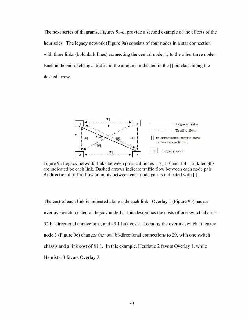
59

The next series of diagrams, Figures 9a-d, provide a second example of the effects of the

heuristics. The legacy network (Figure 9a) consists of four nodes in a star connection

with three links (bold dark lines) connecting the central node, 1, to the other three nodes.

Each node pair exchanges traffic in the amounts indicated in the [] brackets along the

dashed arrow.

The cost of each link is indicated along side each link. Overlay 1 (Figure 9b) has an

overlay switch located on legacy node 1. This design has the costs of one switch chassis,

32 bi-directional connections, and 49.1 link costs. Locating the overlay switch at legacy

node 3 (Figure 9c) changes the total bi-directional connections to 29, with one switch

chassis and a link cost of 81.1. In this example, Heuristic 2 favors Overlay 1, while

Heuristic 3 favors Overlay 2.

Figure 9a Legacy network, links between physical nodes 1-2, 1-3 and 1-4. Link lengths are indicated be each link. Dashed arrows indicate traffic flow between each node pair. Bi-directional traffic flow amounts between each node pair is indicated with [ ].

60

Figure 9b Overlay 1 - Overlay switch at node 1 with logical links 1-2, 1-4 and 1-3 indicated by the bold dashed link. Bi-directional traffic flow as indicated by dashed arrow. There will be a total of 32 connections through the overlay switch as node 1. Link units will be 1* [9] + [10] * 1.41 + [13] * 2 = 49.1. One switch chassis, 32 connections and link costs of 49.1.

Figure 9c Overlay 2 - overlay switch at node 3. Logical links are connected with bold dashed line. Bi-directional traffic flows are indicated with lighter dashed arrows. Logical link 1-3 has a cost of 2, logical link 3-2 has a cost of 3 since the actual path will be 3-1 and 1-2 and logical link 3-4 will have a cost of 3.41, the sum of physical path 3-1 and 1-4. 2*[10] + 3 *[9] + 3.41*[10] = 81.1. One switch chassis, with 29 connections into and out of the switch at 3 and link cost of 81.1.

61

In Overlay1, the overlay switch was placed at node 1 with three links connecting directly

to it where in Overlay 2 the switch was at node 3 where only one legacy link connected

directly to it. This latter design, Overlay 2, created longer path distances for the traffic

flows. Route distances increased from 4.41 to 8.41 units and the link cost requirements

went from 49.1 link units in Overlay 1 to 81.1 link units in Overlay 2. This increase in

link units is largely due to the requirement that all traffic flow move through the overlay

switch at node 3 in Overlay 2 and the one legacy link connecting node 3 to the network.

The violation of heuristic 2 resulted in higher link distances that caused a greater cost.

All traffic must travel over the 1-3 legacy link creating inefficient routing and thus the

greater link cost than for Overlay 1. Overlay 2 (Figure 9c) illustrates a reduction in the

traffic flow from 32 to 29 connections needed at the switch because the overlay switch is

Figure 9d Overlay 3 - Overlay 3 has switches at all four nodes and direct logical full mesh connections between each node pair. Each switch will only handle the traffic that is sourced by or destined for that node.

62

located at the node with high traffic flow demands. The traffic flow demand associated

with the node location of the overlay switch is routed only once through the switch.

Given a different link cost structure, legacy network configuration, or traffic matrix,

locating the overlay switch at the legacy node with higher traffic demands could at times

be the better choice.

Finally, Figure 9d shows an example of a full logical link mesh overlay, Overlay 3.

There will be a total of 42 connections at the switches, four switch chassis (one at each

node) and 49.1 link units in this overlay design, thus creating a more costly design than

Overlay 1 (Figure 9b). The full logical link mesh overlay creates the lowest link costs

when the logical links are along the shortest path between each communicating node pair.

While link costs of this overlay design are the lowest for this legacy topology, each node

will have an overlay switch and each switch will have connection charges. With this

particular legacy design, a 4-node star, with one link connecting each of the three access

nodes to a single core switch, the full logical link mesh overlay will not be the lowest cost

design even though it will have the lowest link costs, equal to that in Overlay 1.

Summary

A mathematical model for the cost of a new service overlay was presented and analyzed.

The relationship between the parts of the model, link and switch costs, was discussed and

arguments as to when each part might dominate the total cost function were presented.

Finally, three design heuristics were defined that can tend to help drive down the total

overlay cost. The three heuristics are first, locate overlay switches at nodes in the center

of the legacy network as opposed to the periphery; second, locate overlay switches at

63

legacy nodes with high connectivity; and third, locate overlay switches at legacy nodes

with high traffic flow demands. The design heuristics presented in this chapter are

guidelines to making choices of where to locate overlay switches for the overlay

backbone. Understanding the legacy network characteristics of topology and traffic

matrix will be required to successfully implant a low cost overlay solution.

64

Chapter 4 Experimental Methods

This research investigates the impact of nodal distribution strategy upon the long-term

cost of a new service overlay installed on an existing legacy telecommunications

network. A byproduct of examining different overlay design strategies is the

development of efficient cost frontiers comparison of network designs. In this chapter an

outline of a set of experiments conducted with a linear programming (LP) problem

formulation of the service overlay with growth problem (SOGP) is presented. Using this

formulation the optimal solution for the overlay was described for several different

network legacy topologies. By manually controlling the node input to the problem,

various nodal distribution strategies for the overlay were examined for four case study

legacy networks. The basic assumption in this investigation for this problem was that an

underlying legacy network topology (nodes and connections between nodes) exists. A

new service overlay will be built on top of the existing network structure with no

additional physical links or nodes added to the legacy physical topology. Thus allowing

traffic flows of the new service to be transmitted over the existing topology.

Service Overlay with Growth Problem [SOGP] Formulation

Definitions:

• n is the number of nodes, N is the set of such nodes. N = {1, 2, 3, … , n} = i = j. • A is the set of possible bi-directional edges in the graph on the set of nodes N.• T is the set of time periods, t, in the study. T = {1, 2, … , t}.

65

• Dt is the set of all non-zero flow demand quantities exchanged between nodes, indexed by r. D will be different for each time period t. The elements of Dt

represent the traffic to be carried by the network for each city pair. • drt is the amount of flow demand associated with the rth demand pair in D for

period, t. • O[r] is the node that is the origin for the rth flow demand pair in D.• TR[r] is the corresponding target or destination. • clij (= clji) is the incremental cost of adding one unit of capacity to edge (i,j).

These incremental steps can be the same or different for each time period. • wrt

ij is the amount of working flow of the rth demand routed between nodes (i,j) on link i,j or j,i for period t.

• lwijt is the working capacity assigned to the edge between nodes (i,j) to support all

working flows routed over that edge for period t. • Sjk is the fixed cost of a switch at node j. There are incremental steps, k, in this

function determined by the number of ports needed to carry all the traffic flow coming through and into the switch at node j. These incremental steps can be the same or different for each time period. The value of Sjk at each increment of k will be arbitrarily defined.

• cpj is the incremental cost of adding one unit of capacity to switch at node j. These incremental costs can be the same or different for each time period.

• Pjt = the number of connections needed in switch at node j to accommodate all the

traffic flow that will enter or leave this switch. It is the sum of the demand flow routed to/from and through node j.

• CSjk is the incremental cost of the switch chassis. CSjk is a constant value set before the model is analyzed. These incremental costs can be the same or different for each time period. This formulation has them the same for each node.

• K is the set of incremental costs, k corresponding to the number of different sizes of chassis used in the model, b.. K = {0, 1, 2, …, k}.

• CNjk is the maximum number of connections that any switch size will allow. For each k there will be a predefined constant such as 1000, depending on the size of the switch chassis.

• M is an arbitrarily large constant that is greater than any capacity needed to accommodate all the flow through a switch.

• zjk is a binary variable (0,1) used to facilitate the step cost function of the switch chassis. The number of different sizes of the chassis, b, is the number of different values for the subscript k. K ={0,1,2, …, k). zjk will be 1 for the appropriate size of Pj and zero for the rest. Only one chassis will be installed at each node. When k = 0 there are no (0) connections for that nodes and therefore no switch at that nodes.

• xj is a binary variable (0,1) used to control the nodes that are allowed to have a switch in the design. This variable can be manually controlled.

66

Objective Statement: Min Σ { Σ xj Sj

t + Σ xj {cpjt * Pj

t } + Σ {clijt *lwij

t}} 4.1 t∈T j∈N j∈N i,j∈ A

Subject to: Σ wrt

ij - Σ wrtji = drt for all r ∈ D, i = O[r] and for all t∈T. 4.2

j∈ A j∈ A

Σ wrtij - Σ wrt

ji = - drt for all r ∈ D, i = TR[r] and for all t∈T. 4.3 j∈ A j∈ A

Σ wrtij - Σ wrt

ji = 0 for all r ∈ D, for all i ∉ {O [r] or TR[r] } and for all t∈T. 4.4 j∈ A j∈ A

lwijt = Σ wrt

ij + Σ wrtji for all i,j∈ A and for all t ∈ T. 4.5

i,j∈ A j,i∈ A

Pjt = lwij

t + lwjit for all i,j∈ A and for all t ∈ T. 4.6

Pjt <= M * (zj0 + zj1 + zj2 + … + zjk) 4.7

zjkt ∈ {0,1} for all j∈N, for all i,j ∈ A and for all t∈T . 4.8

Pjt <= 0zj0 + CN1 zj1 + CN2 zj2 + … + CNjk zjk 4.9

Sjt = 0zj0 * CSj0

t + zj1t * CSj1

t + … + zjkt * CSjk

t 4.10 Σ zjk

t = 1, for all j and for all k and for all t ∈ T. 4.11

lwijt - lwij

t-1 >= 0, for all i,j ∈ A and for all t ∈ T. 4.12

wrtij, wrt

ji >= 0. 4.13

4.1 - The objective statement seeks to minimize the cost of the network overlay based on

three factors, the cost of the node/switch chassis, the cost of each connection to the

switch chassis and the cost of additional capacity on a link to support the required flow.

67

4.2, 4.3, 4.4 – These are standard flow balance constraints that require that all the flow

leaves the source, all the flow arrives at the destination and that at all transshipment

nodes the flow is balanced so that all the flow that enters the nodes leaves the node.

4.5 – This constraint, the link capacity constraint, sums all working flow, wrtij, and wrt

ji,

that traverse this link to determine the amount of capacity needed on the link.

4.6 – This constraint is the switch size constraint that sums all working flows that go

though this link to determine the number of connections needed for the switch at node j.

4.7 – This constraint says that the value of Pjt will be either zero if there is not a switch at

this location or it will be less than M that is a number sufficiently larger than any

connection capacity needed at any switch.

4.8 – This statement defines the binary choice variable, zjkt, defined for each node, j, as to

which size of switch chassis is installed at the node.

4.9 - This constraint determine the correct size of switch to be placed at a node based on

the number of connections required to deliver the traffic flow.

4.10 – This constraint calculates the cost of the switch based on the previous constraint

and that since this is a minimization problem the cheapest size will be selected based on

the correct value of zjk from constraint 4.9.

4.11 – This constraint requires that there be only one switch size for each node if any at

all.

4.12 – This constraint requires that the input to the next period, t, be the output of the

pervious period.

4.13 – This constraint states that the working flow, wrtij, and wrt

ji, will be either zero or a

positive number.

68

This formulation modeled after Grover and Doucette 2001 and Chang and Gavish 1993

creates a sum of shortest paths for the traffic flow solution for the input design criteria of

nodes, links and traffic flow values. The implementation of this problem was done using

single sequential periods with the output of the first period being the input to the next.

Plan of Analysis

Step 1: Legacy topology, T0

The initial legacy topology, T0, for proof of concept testing was a 9-node model (Figure

10) (see Appendix A for details).

Figure 10 – Initial 9 node proof of concept model

69

Three case studies then were conducted using a generic North American network based

on that of WilTel (Figure 11), the NSFNet from the US research network, the beginnings

of the Internet (Figure 12), and a generic Pan-European model based on that used in

Maesschalck et al, 2003 (Figure 13). The North American network has 27 nodes and 43

links. The Pan-European network has 28 nodes and 43 links. The NSFNet network

model has 15 nodes and 22 links. The location and populations details for each of the

case studies are included in Appendix A.

Figure 11 The North American legacy topology based on the WilTel North American network. The number by each city name is an index. The details of population, location, and link length are in Appendix A.

70

Figure 12 The NSFNet legacy topology. The number by each city is an index. The details of population, location, and link length are in Appendix A.

Figure 13 Pan-European legacy topology. The number by each city is an index. The details of population, location, and link length are in Appendix A.

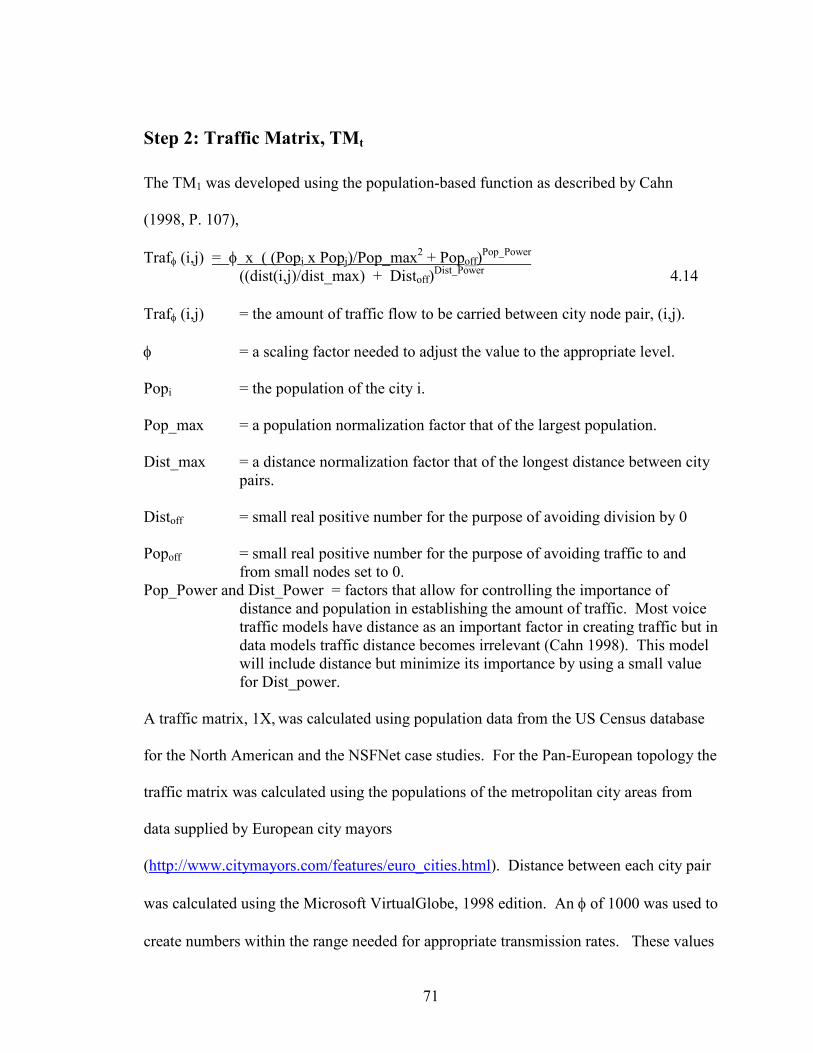
71

Step 2: Traffic Matrix, TMt

The TM1 was developed using the population-based function as described by Cahn

(1998, P. 107),

Trafφ (i,j) = φ x ( (Popi x Popj)/Pop_max2 + Popoff)Pop_Power

((dist(i,j)/dist_max) + Distoff)Dist_Power 4.14

Trafφ (i,j) = the amount of traffic flow to be carried between city node pair, (i,j). φ = a scaling factor needed to adjust the value to the appropriate level. Popi = the population of the city i. Pop_max = a population normalization factor that of the largest population. Dist_max = a distance normalization factor that of the longest distance between city

pairs. Distoff = small real positive number for the purpose of avoiding division by 0 Popoff = small real positive number for the purpose of avoiding traffic to and

from small nodes set to 0. Pop_Power and Dist_Power = factors that allow for controlling the importance of

distance and population in establishing the amount of traffic. Most voice traffic models have distance as an important factor in creating traffic but in data models traffic distance becomes irrelevant (Cahn 1998). This model will include distance but minimize its importance by using a small value for Dist_power.

A traffic matrix, 1X, was calculated using population data from the US Census database

for the North American and the NSFNet case studies. For the Pan-European topology the

traffic matrix was calculated using the populations of the metropolitan city areas from

data supplied by European city mayors

(http://www.citymayors.com/features/euro_cities.html). Distance between each city pair

was calculated using the Microsoft VirtualGlobe, 1998 edition. An φ of 1000 was used to

create numbers within the range needed for appropriate transmission rates. These values

72

were then translated from bits per sec (bps) into the number of Digital Signal 3, DS3,

needed. For example, in the North American case study, from Seattle (node 1) to San

Francisco (node 2), have populations of 3.6 million and 7 million respectively. The

distance between the two is 1084 miles. Using the formula presented above a value of

.1623 is calculated, with α=1000, scaled value of 162.3 is created. This number is 162.3

million bps. Dividing 162.3 million bps by 45 million bps, the approximate value of a

DS3, gives 3.6 DS3 or rounded to 4 DS3. The amount of traffic flow to be carried

between node 1 and node 2 on the North American case study for the 1X growth stage

would be 4 DS3s. Once the input parameters were established a full traffic flow matrix

was calculated and the traffic values are included in Appendix B.

Step 3: Cost Models

The cost models for the overlay were developed using generic cost functions based on

data from previously published data from WilTel and other public data. These functions

were built from the carrier perspective, essentially, the cost required to implement the

new service overlay. Other cost functions can be developed to emphasize other

perspectives such as that of expected revenue or cost to the customer. Different cost

structures can produce different results from those seen in this study.

There were three cost functions used in this study, the cost of capacity on a link, the cost

of the switch chassis and the cost of each flow connection in and out of the switch

chassis. Each unit of connection in the switch is a constant cost which in this study was

set to 125. The actual switch chassis costs are a step function that is not generally linear

and were set to $1000, $2000, $4000, $10000, and $20000 with switch sizes set to 1000

73

ports, 2000 ports, 4000 ports, 12000 ports, and 24000 ports. Larger switches while

overall more costly show a decrease in cost per unit.

Each unit of link cost is a function of the distance of the link and the link capacity times a

dollar amount. The distance was determined by summing the linear distances between

the end legacy nodes traversed by the overlay link. For this study to keep link costs

simple, the dollar amount was arbitrarily set to $1 pr distance unit. Capacity multiplied

by distance and by the unit link cost created the total link cost for each link.

Step 4: Develop “Best” network topology

MPL, Maximal, Inc. software was used to implement the linear programming (LP)

formulation of the SOGP and the single “best” design for the input parameters was

calculated. This model was implemented in single sequential periods with the topology

output, including number, location and size of switches, the links and the capacity of

links of one growth period as the input for the next growth period. The difference

between each period was the increase in the amount of traffic. The actual MPL

implementation of the SOGP is presented in Appendix C. In the MPL implementation,

chassis and ports were allowed at all nodes including all the access nodes. These access

node costs, chassis and ports, were manually deducted from the final costs to determine

the final total cost for the overlay design.

74

Step 5: Analyze the impact of nodal distribution – create efficient

frontiers

To understand the impact of overlay switch/nodal distribution upon long-term cost, the

number and distribution of switches in the service overlay were manually varied using

different design strategies developed around both number of switches, node population

size and location of the nodes in the backbone. To approximate network growth a five

level traffic matrix was developed. 1X growth stage represented the traffic matrix

calculated as described in Step 2 of this chapter. Four additional growth stages were

calculated by multiplying the initial amount of traffic demand, 1X growth stage, by 1.5,

3.5 and 10 creating five growth stages 1X, 1.5X, 3X, 5X, and 10X. For this study each

design strategy was modeled using all five-growth stages.

This study was to examine not only the impact of number of switches in the service

overlay for long term growth potential but the location and size of the nodes as well. For

each case study several one and two switch designs were calculated. The location of the

backbone design for each scenario was established using the shortest path connections

between each backbone node. From these analyses, a series of total costs for each traffic

growth stage were developed. Other scenarios were developed having more switches

included in the overlay backbone. The variations were based on the design heuristics of

Chapter 3 and included not only the number of overlay switches but location, periphery

versus central locations and population of the node. To control the population variable

three groups of nodes were established based on population size of the city at the node,

small, medium, and large, for each real world case study. The details of the three groups

are presented in Appendix A.

75

Summary

In summary, a LP formulation of the SOGP using a combination of relevant portions of

several previously defined LP models was used. A single sequential period approach was

used by manually controlling the input to sequential periods. This model was validated

using a proof-of-concept 9-node model (Figure 10). Three case studies were developed,

a North American topology (Figure 11), the NSFNet topology (Figure 12), and a Pan-

European topology (Figure 13). A series of traffic models based on initial data modified

by population density heuristics were calculated. These inputs were used in the SOGP

and the optimal network designs were calculated. The inclusion of nodes in the backbone

of the overlay was manually controlled to create scenarios of different node distributions

in the service overlay. Nodes were chosen based on population of the city, location (near

the center of the network or near the periphery), and legacy network connectivity at the

node site. A series of total costs for each configuration for each growth stage was

calculated.

76

Chapter 5 Results of Case Studies Analyses

Using the mathematical model described in Chapter 3 and as implemented by the SOGP

formulation described in Chapter 4, four separate case studies were evaluated, first, a

small proof-of-concept 9-node legacy network (Figure 10) and then three larger closer-to-

real-world legacy models, a North American, NA, model (Figure 11), the NSFNet

(Figure 12), and a Pan-European, PE, model (Figure 13). This chapter presents the

results of the experimental analyses and compares the results to the design heuristics

discussed in Chapter 3.

The primary backbone design strategy used to develop test network configurations used

the philosophy that once a legacy node was in the overlay backbone the overlay switch

handled all traffic flows that went through this node. Hereafter this will be referred to as

design strategy 1. A secondary strategy 2 created a mesh topology with logical links

between each node pair in the overlay backbone. The only traffic flow handled by an

overlay switch in the full logical link mesh is traffic flow that originates and terminates at

that switch location. Those nodes not in the overlay backbone will have access to the

nearest overlay backbone switch and that switch will handle (originate and terminate)

their traffic flow. Thru traffic flow that passes through a node with an overlay switch

will be processed by the assets of the underlying legacy network. Hereafter this will be

referred to as design strategy 2. A limited number of mixed topologies, using a

combination of legacy and logical links, were also evaluated.

77

Figure 14 – Backbone design strategies using logical links or legacy links. Backbone Design Strategy 1 – Legacy Links- once a node is in the overlay all traffic flows that move through that node are seen by the overlay switch. In this design there are two logical links that carry traffic flows and all traffic flows will move through the overlay switch at node 2 Backbone Design Strategy 2 – Logical Links - while there are switches at all three nodes, there are three logical links, one between each legacy node pair. The overlay switch at node 2 only handles the traffic flows that start or end at node 2.

Growth Studies - Scalability

One of the original goals of this study was to examine design strategies for long-term

growth and the impact of growth on the most cost effective design. A series of traffic

flow models were chosen to approximate long-term growth. The 1X growth stage

represented initial traffic as calculated by the formula presented in Chapter 4, equation

4.14. Sequential growth stages were a multiplication of that initial traffic flow matrix by

a scale factor, 1.5X, 3X, 5X and 10X. Using the linear programming formulation, SOGP,

defined in Chapter 4, the most cost effective overlay design for the initial 1X growth

stage was the most cost effective design for all of the sequential growth stages of designs

78

evaluated. The price structure used in this set of experiments did not feature economy of

scale regarding link costs. Doubling the required link bandwidth doubled the costs.

Overlay switch costs did show economy of scale savings, but only when heavy traffic

loads were processed. This cost structure did not warrant any radical overlay redesigns

as the network traffic increased. Future research could be done using link economies of

scale that might show different behaviors than those seen in this study as far as the impact

of growth on the total cost of an overlay.

The 9-node Case Study

The 9-node network topology presented in Chapter 4 (Figure 10) is well connected with

an average degree of connectivity of 4.4 and has a high skewness of connectivity of 1.17

(Table 1). Skewness is a measure of symmetry, or more precisely, the lack of symmetry

of a data set (see Appendix C for details of skewness calculation). The distribution of a

data set is symmetric if it looks the same to the left and right of the center point. The

high skewness of the distribution of the degree of nodal connectivity indicates that there

are more nodes with a high degree of connectivity than those of average or lower degree

of connectivity. Link distances for this model are a value of 1 or 2 with an average of 1.4

and the switch costs are an arbitrary 10, 20, 30, 40 and 50 for sizes of 50, 100, 200, and

500 connections respectively (See Appendix A for details). The unit cost constants of

switch costs, KS, are much greater than link costs, KL, KS >> KL.

79

NetworkNodes C C Pop Links

Link length

# Average Skewness Ave in

M # (Mean) 9 node 9 4.44 1.17 NA 20 1.40PE 28 3.04 0.73 1.42 43 248.21NA 27 2.93 0.14 3.79 43 436.95NSFNet 15 3.19 0.28 3.92 22 1085.45

Table 1. Network characteristics of case study legacy networks. Network characteristics of number of nodes, connectivity of nodes, population of nodes, number of links, link length are presented in this table. Statistical values were calculated using the descriptive analysis package for data analysis in Microsoft Excel. C is the connectivity of the nodes in the network.

The most cost effective overlay design evaluated for this model is the one switch

centralized in a star pattern (Figure 15). For this case study two different one-switch

scenarios were evaluated. The location of the one switch is very important. First, the

switch was located at the most central node of the legacy network and second at a

periphery node. The central node location was the most cost effective design evaluated.

Locating the overlay switch at a periphery node increased the link costs due to increased

backhaul distances. An intermediate distribution of nearly 45% (4 out of 9) of the legacy

nodes in the service overlay is the next most cost effective long-term approach evaluated.

80

Figure 15 Experimental total cost results for the 9-node legacy network. One switch on a central location was the lowest cost solution evaluated by this study while one node switch located at a periphery location was more costly.

For this 9-node legacy topology, two overlay designs with switches at all nodes were

evaluated using both design strategies. There were switches at all nodes with logical

links between all nodes, as per design strategy 2, and the other design used the links of

the legacy topology, as per design strategy 1. These two designs have minimized link

costs because all traffic flow paths are available so the sum of traffic flow paths will be

minimal. Each design will have the same number of overlay switch chassis but the

number of connections per switch will be different. The design with logical links will

have the minimal number of connections because the overlay switches will handle only

local traffic flows and no pass through traffic flow, so the switch chassis will be of the

81

smallest size possible. For this 9-node legacy network the backbone design strategy

creating a full logical link mesh becomes the lower cost design evaluated for overlay

switches distributed over all legacy nodes.

The cost function for this legacy network is dominated by the cost of switches including

both chassis and port costs, as well as the unit cost of switches being much greater than

the unit costs of links, KS >> KL. Link distances, as well, were minimal and therefore

had limited impact upon the total cost. For this type of network design where total switch

costs are dominant, total network costs tend to be impacted first by switch costs. Once

switch costs are minimized then link costs need to be addressed. A centralized node

location with one switch that has high connectivity is the lowest cost design evaluated for

this legacy network (Figure 15). As the overlay design strategy includes switches at

more legacy nodes, the total switch cost increases and therefore the total design cost

increases. The efficient frontier for this legacy topology connects the low cost one-

switch scenario, which for this study is the lowest cost design; to the intermediate

distribution design and then to the full mesh logical link design. For this legacy

topology, a centralized distribution will tend to be the lowest cost solution with

increasing costs as more nodes are added.

Two of the design heuristics, place overlay switches at legacy node locations with high

connectivity and at central rather than periphery legacy locations, are reflected in the

results of this case study. The centralized location of the one switch in the low cost

design is at a location of high connectivity, which also reduces backhaul of traffic flows

and minimizes link costs. Also, most traffic flow is carried directly to the switch because

82

the central node with the overlay switch is directly connected to all of the other nodes.

So traffic flow is routed efficiently and backhaul distance of traffic flow is minimal. The

centralized location of the one switch in the low cost design is at a location of high

connectivity, which also reduces backhaul of traffic flows and minimizes link costs.

North American and NSFNet Case Studies

The North American, NA, and the NSFNet models have network characteristics of longer

link distances, average of 437 miles and 1085 respectively and lower skewness of

connectivity of nodes, 0.14 and 0.28 respectively (Table 1) (see Appendix A for details).

For the implementation of these network designs the unit cost of link capacity was set to

1, KL = 1. While the unit cost of switches, KS, is much greater than the unit cost of links,

KL, the long link distances result in the dominant factor being the cost of links.

The total link costs for the NA overlay designs evaluated range from $30 Million to less

than $80 Million while total switch costs were in the range of $5 Million to less than $30

Million. For the NSFNet case study the link cost range was between $10 and $40 Million

and switch cost range was between $1 and $6 Million. As mentioned previously, link

costs tend to dominate the total cost for these two legacy topologies (Figure 16). The key

to minimizing costs for these case studies is to focus on minimizing link costs.

83

Figure 16 Switch verses Link Costs. Switch costs were plotted against link costs for the three real-world case study networks.

For both these network case studies, the fully distributed switch approach with a full

logical link mesh overlay and a switch at every node following backbone design strategy

2 is the most cost effective design evaluated (Figure 17 and 19). Link cost functions due

to the long link lengths dominate the total cost function for these case study legacy

topologies. The cost structure used in these experiments, coupled with the long link

distances, tilts the low cost advantage towards highly connected overlay networks. As

noted in Chapter 3, the cost structure used does not offer any economy of scale benefits

for high capacity links. Doubling a link capacity doubles the cost. Hence, aggregating

flows onto a reduced number of high capacity but possibly more roundabout overlay

trunk paths offers no potential savings.

84

A full mesh overlay that uses the shortest path connections between each node pair has

the smallest possible total link capacity requirement of all possible network designs

[Cahn, 1998]. For example, if a direct logical link carrying B units of traffic between two

nodes is removed from a full mesh overlay, the traffic carried by the network decreases

by B units. But this traffic must still be carried between the two end nodes. If rerouted

over a two hop path, B additional units of traffic will now have to be carried over two

pre-existing links instead of one direct link. The total amount of traffic carried by the

overlay network will increase by B units- B units were saved by eliminating the direct

link, but 2B units were added. Note also that the total switch ports required by the

overlay network will also increase, by 2B units. A relay switch will need an increased

capacity of B units on two links.

With this cost structure, traffic flow paths need to be minimal for link costs to be

minimized. In these experiments, all logical links on a full mesh overlay network are

routed over the shortest path. Depending on the configuration of the underlying legacy

network, in the above example, the total distance that any rerouted traffic must be hauled

may increase. Rerouted traffic will never travel a shorter distance than direct traffic. At

best, it will remain the same. The overall impact of this is that a full mesh overlay

network will have the minimum possible link cost for the cost structure used in these

experiments. At best, an alternative overlay network can have the same link cost of a full

mesh, but not less.

A full mesh overlay will not necessarily have the smallest total switch cost. Though if an

overlay switch is placed at every legacy node, the full logical link mesh switch cost will

85

be the lowest because the number of connections in each switch will be minimal since

each switch will only handle the traffic flow from the legacy node. A partial overlay

mesh will require an increased number of ports to handle relay traffic. Completely

eliminating overlay switches except for one core switch has the potential to reduce switch

cost dramatically. Figure 9 in chapter 3 shows some examples. With the cost structure

used in these experiments, full logical mesh designs will not always be the lowest cost for

all legacy network topologies. For example, in the design of Figure 9d the full logical

mesh is not the lowest cost design.

Figure 17 North American Legacy Overlay Design studies. All of the five growth stages are presented but the efficient frontier is drawn only for the 10X growth period. Lowest cost design strategies evaluated for this study are the distributed overlays with switches at all or most nodes.

86

Figure 18 NSFNet Legacy Overlay Design studies. All of the five growth stages are presented but the efficient frontier is drawn only for the 10X growth period. Lowest cost design strategies evaluated are the distributed with switches at all or most nodes.

Some combinations of traffic flows over adjacent routes and elimination of certain

switches may result in lower total cost designs those evaluated in Figures 18 and 19.

Careful application of the heuristics described in Chapter 3 should point the way to a

lower cost design. Certain nodes would be made access only and not a part of the overlay

backbone based on choices made due to the design heuristics. The increase in traffic

flow paths and therefore the increase in link cost could possibly be offset by the reduction

in switch costs. However, as this is an intractable NP-hard problem, the only sure way to

find a lower cost design is via exhaustive testing of alternate overlay configurations,

guided by the design heuristics.

87

Two additional logical link designs for the NA case study with fewer switches in the

overlay backbone were analyzed. A full logical link mesh design with only 26 nodes in

the overlay backbone was constructed. Node 27 (Albany) was removed from the overlay

backbone with its only access to the overlay the link to node 25 (New York, see Figure

11). Node 27 has one of the smallest traffic flow demands for this case study, is a

periphery node and has a connectivity of 3. Analysis of this design showed that while the

total switch costs of the 26-node overlay with full logical mesh connectivity were less

than that of the 27-node design, link costs increased more than enough to offset the

decrease in switch costs. The total cost of the 26-node overlay was larger than that of the

27-node overlay design. The second logical link design removed four nodes from the

overlay backbone that were 2-degree connectivity nodes, specifically nodes 1 (Seattle),

15 (Minneapolis), 22 (Miami), and 26 (Boston). These four nodes are in the middle to

large population groups (Appendix A). This design had 23 switches in the overlay

backbone and resulted in a larger total cost than the fully distributed approach due to

increases in link costs that offset decreases in switch costs.

For the NA designs evaluated in this study, the designs with switches at most or all nodes

tend to be the lower cost. The key to this trend may be both the long link lengths and the

low connectivity of the nodes of the legacy NA and NSFNet designs. The low nodal

connectivity does not allow many path choices thus total path lengths between overlay

designs may be similar. The dominant link costs in this model due to the longer link

lengths must be minimized for total cost to be minimized. While the lowest total cost

designs evaluated for this study for both the NA case study and the NSFNet were the

88

lowest link cost they were not the lowest switch cost (Figure 16) indicating that link costs

drove total cost with this legacy topology and the factors used in this study.

The efficient frontiers, suites of best evaluated in this study, for both of these designs are

approximately linear decreasing from one switch to switches fully distributed at all nodes

in the legacy network for the NA and NSFNet case studies (Figure 17 and 19). As

previously mentioned, in the NA and NSFNet case studies link costs tend to dominate the

cost function. For the NA and NSFNet topologies increases in switch costs are offset by

decreases in link costs. Increased link costs in more centralized one-switch overlay

designs are due to increased amounts of backhaul of traffic flows. These increased link

costs offset the decrease in switch costs with fewer overlay switches.

The impact of the design heuristics can most easily be seen in the total costs of one-

switch overlay designs in all three case studies. In Figure 19 the costs of all the one-

switch overlay designs for each case study evaluated were plotted against the

connectivity of the underlying legacy node. For each case study, the lowest cost one-

switch design evaluated was located at a central and well-connected legacy location in

the set of designs evaluated. Population or the level of traffic flow demands originating

and terminating at the switch location was not the deciding factor in cost for the designs

evaluated in this study. Central location along with connectivity seem to be more

important factors in total cost, for the designs studied, than the amount of traffic flow

demand associated with the legacy node. While the number of designs for each case

study was limited, the interoperations between the heuristics are consistent.

89

Figure 19 One-switch one node design total costs verses connectivity of legacy node. All lowest cost designs evaluated for this study were at central and fairly well connected locations. At least for these designs evaluated population or traffic demands were not a major deciding factor.

The impact of the design heuristics is also seen in the multimode designs of in the NA

case study, albeit more subtly. Points labeled A-D in Figure 17 have approximately 1/3

of the total legacy nodes in the overlay backbone. The nodes of point A are the large

population nodes. The nodes of point B are from the medium population group and the

nodes of point C are the small population group (See Appendix A for details). The

overlay backbones for these three designs were relatively minimally connected with

mostly 2-degree connectivity between each overlay backbone node. These designs were

constructed to essentially indicate the impact of design heuristic 3, place overlay switches

at legacy nodes with large traffic demands. For the purposes of this study, population of

90

the legacy node was assumed to indicate traffic demand, i.e. large population generates

large traffic demands. While the total cost of these three designs was very similar there

were some differences, the design with the high population was the lowest cost of the

three designs and the design with the smallest population was the highest cost.

Considering only traffic flow demands, at least with these three scenarios, the traffic

demand of legacy nodes used in the overlay backbone has a limited impact upon the total

cost of the overlay.

Point D has similar number of switches in the overlay backbone as the previous

discussion but control factor for this design was that the legacy nodes in the overlay

backbone had to have a high connectivity. Each legacy node included in the overlay

backbone had a 4 or 5-degree connectivity. This design created a backbone with much

higher connectivity than designs A-C and the total cost of design D was much less than

that for designs A-C. The strategy associated with design D was to evaluate heuristic 2,

locate overlay switches at legacy nodes with high connectivity. Comparing the designs A

– D, the number of nodes in the backbone does not seem to be a dominant factor in the

total cost of the overlay but the connectivity of the overlay backbone is important.

Population of the legacy node seems to have some, albeit limited, impact so design

heuristic 3 is also supported.

Designs associated with points E, F, and G had 13 nodes in the overlay, approximately ½

of the legacy nodes in the NA case study. Point E had overlay backbone switches at 8

large population nodes and 5 small nodes. Points F and G are associated with two

backbone variations using the same set of legacy nodes, 8 large population nodes and 5

91

medium population nodes. The difference between the two designs is the connectivity of

the overlay backbone. The design associated with point G had nodes located at legacy

locations with higher connectivity than that associated with point F. The impact of

design heuristic 2, locating overlay backbone nodes at locations of high connectivity, is

seen with this scenario. Design heuristic 3, locate overlay switches at legacy nodes with

high traffic flow demands, is also seen in this analysis as the design with the small

population nodes, point E, as compared to the other two, has the higher cost.

Designs H, I, and J have switches at approximately 2/3 of the NA case study legacy

nodes. These designs were constructed to compare the impact of number of overlay

switches in the overlay backbone, traffic demands, and backbone connectivity. In design

H, all large population nodes were eliminated so switches were placed at only the 9 small

population nodes and 10 medium population nodes. This design had relatively poor

connectivity with an average degree of connectivity of 1.8. Design I had overlay

switches at the 10 medium population nodes and the 8 large population nodes. The

connectivity of this design was an average of 1.7. Finally, design J had a mix of

population sizes and all 2-degree legacy locations were eliminated. This design was

better connected with an average degree of connectivity of 3. The backbone design

strategy used to connect the nodes with switches was that of design strategy 1 explained

at the start of this chapter. Comparing these three designs shows that population of

legacy node or traffic demands generated did have an impact in creating total cost.

Design H with small and medium population nodes in the overlay backbone was much

more costly than design I or J. Design J, a mix of population sizes, was much better

92

connected and had the lowest cost of the three designs. Design heuristics 2 and 3 are

supported by this analysis.

To compare the impact of the two-backbone design strategies designs K and L were

constructed with overlay switches at 23 legacy nodes. The four legacy nodes removed

from the backbone had 2-degree connectivity and were periphery nodes. Design K is

associated with design strategy 1 that included only legacy links in the backbone while

design L was constructed using design strategy 2 of a full logical link mesh. The 23

nodes in the overlay backbone have logical links between each communicating pair and 4

nodes had only access connections to the nearest overlay backbone node. Both designs

have the same link costs, which would be the sum of shortest path for each traffic

demand, but different switch costs. Design L switch costs are less than those of design K

because design L has logical mesh links between all nodes on the overlay backbone. The

difference between designs K and L is due only to the different design strategy.

Multi-node designs defined for the NSFNet case study show the impact of the design

heuristics in a similar manner. The size of the population of the nodes included in the

overlay backbone had some impact in total cost comparison. Having nodes with the

larger populations in the overlay backbone did produce somewhat lower cost total

designs as compared to the designs with nodes of smaller population in the overlay. For

the designs evaluated connectivity of the overlay backbone was a more important factor.

The higher the connectivity of the nodes in the overlay backbone the lower the total cost

of the design. Both design heuristics 2 and 3 are supported by the multi-node cases of the

NSFNet case study.

93

Pan-European Model Case Study

Key topology characteristics of the Pan-European, PE, network are shorter link distances

than NA or NSFNet and more nodes with high connectivity as shown by the high

skewness of connectivity of nodes (Table 1). For the PE model network designs, the unit

cost of link capacity was set to 1, KL = 1. The unit cost for switches, KS, was the same as

defined for the NA and the NSFNet models, so KS >> KL. For the designs evaluated in

this case study, the range of switch costs was from $3 to 15 Million while the range for

link costs was $10-30 Million (Figure 16). The differences between switch and link costs

of the designs evaluated in this study are much less than the other two larger case studies

and in some instances actually are very similar. Among the designs evaluated for this

research, the full logical mesh overlay was again the lowest cost design (Figure 19).

94

Figure 20 Pan-European Legacy Network overlay design studies. Five traffic demand growth periods for each design scenario were modeled. The efficient frontier is drawn only on the 10X data. The solid line indicates the efficient frontier for the designs with full logical link mesh overlays, design strategy 2. For design strategy 1 that utilized the direct links of the legacy topology the efficient frontier is a dashed line.

The one-switch overlay approach was the next most cost effective design evaluated in

this study but the location of the overlay switch was critical (Figure 20). A central

location of high connectivity was important in lowering the total cost of the overlay.

There are several possible reasons for this. First, the location of the switch at a

centralized node in the legacy network is important because link distances tend to be

minimized which in turn minimizes backhaul costs. Periphery locations for a switch

require longer flow paths thus increasing the distance traffic flow must be backhauled.

The degree of connectivity for the periphery location also has an effect upon the total

95

cost, the higher the connectivity of the switch location, the lower the total cost of the

overlay.

For the lower cost one-switch overlay designs evaluated in this study, traffic volume from

the node location was not an important factor in influencing total cost. The lowest cost

one-switch overlay design had the switch located at node 14 (Frankfurt, see Figure 9).

This location ranked 21 out of 28 in population size but was a centralized node location

with a degree of connectivity of 5. Periphery locations of similar connectivity to that of

node 14 but with higher traffic flow demands showed a somewhat higher total cost. This

implies that the volume of traffic flow from any given node, while important to the total

overall cost, at least for designs evaluated, was less important than minimizing backhaul

distances.

The efficient frontier for this case study when drawn to include the full logical link mesh

shows the lower cost designs to have more switches distributed over the full PE legacy

network (Figure 20). When using design strategy 1 with all switches on the backbone

handling all traffic moving through the node to draw the efficient frontier, the opposite

relationship is seen. Centralized switch designs tend to be less costly when using design

strategy 1 for the PE legacy network evaluated. Were the design strategy 2 applied to

overlay backbones consisting of a smaller number of overlay switches, designs with costs

lower than that of the single node designs, but in most cases higher than that of the full

mesh, are to be expected. Patiently applying the design heuristics could show other

designs that may have lower costs than any of the examined configurations, but since this

is an intractable NP-hard problem it might very well require extensive analyses. The

96

network designer using the design heuristics, knowledge of the traffic flow matrix, and

other undefined model constraints could develop a set of designs that define a more

continuous efficient frontier for the problem.

The lowest cost one-switch overlay design among those studied in this research has the

switch at a central node of fairly high connectivity, degree 5 (Figure 20). This is

consistent with the heuristics that recommend locating overlay switches at nodes of high

connectivity on the legacy layer and locating the overlay switch in the central part of the

legacy network. This design strategy also reduced backhaul distance of traffic flow by

having the switch located at a centrally located node. Locating switches at nodes of high

traffic flow can still impact total cost but minimizing backhaul distance in this case was

an over riding factor.

Comparison of multi-node designs for the PE case study using 13 nodes in the overlay

backbone showed similar impact of the design heuristics, as did the multi-node overlay

designs for the NA and NSFNet case studies. For the multi-node designs studies

population size of the node again had less of an apparent impact than the connectivity of

the node in effecting the total cost of the overlay.

Summary

Defining the lowest cost overlay for a legacy network will depend upon the relative value

of link cost to switch cost, the traffic flow demands, and the connectivity of the network.

When switch costs dominate, minimizing switch costs is the first key to keeping the total

cost down. For other topologies where link costs dominate the number of switches

becomes less of a factor in the total cost function than minimizing link costs.

97

Determining the dominant influence in the cost function will be the key to minimizing

costs and predicting the shape of the efficient frontier. The results of the four case

studies analyzed for this dissertation are consistent with the three heuristics presented in

Chapter 3 with the cost structure tested except that traffic flow demands had less of an

impact upon reducing costs as compared to centralized location and connectivity.

Efficient frontiers for each case study, based on the designs evaluated, were drawn

indicating that for the NA and NSFNet case studies the distributed approach with

switches at more nodes tend to be more cost efficient, regardless of whether design

strategy 1 or 2 is used. For the PE topology case study, based on the designs evaluated

for this study, the two design strategies produce different results. Using design strategy 2

with a full logical link mesh design switches at every legacy node was the lowest cost

design. If that design philosophy is not used, then a single switch that is located at a

central highly connected node is the more cost effective.

98

Chapter 6 Summary and Future Research

Summary

This research looked at design issues associated with building an overlay network on top

of an existing legacy network with overlay network switches and links not necessarily

matching the switch and link locations of the underlying network. While there are many

studies that present methods to define low cost network designs, there are few studies that

define an overlay network that dos not necessarily match the topology of the underlying

network. Since this is an intractable NP-hard problem and finding the optimal solution is

not always feasible, three design heuristics were presented that can help guide the

network designer to developing low cost solutions. Also to examine the impact in

changing network designs due to real world constraints the concept of efficient frontier

was applied to this problem.

The answer to the question of which design philosophy is better for the service overlay,

that of centralized versus distributed overlay switches, depends upon the characteristics

of the legacy topology and the cost function defined for the overlay. This study

developed a mathematical model that has two basic components, switch costs and link

costs, for defining the total cost of a network overlay. The three heuristics presented can

be used to help point to the direction of keeping costs under control when design changes

are required. The three heuristics are first, locate overlay switches at nodes in the center

99

of the legacy network as opposed to the periphery; second, locate overlay switches at

legacy nodes with high connectivity; and third, locate overlay switches at legacy nodes

with high traffic flow demands. Applying the concept of efficient frontiers to the world of

network design and building a suite of best designs gives the network designer greater

insight into how to design the best network in the face of changing real-world constraints.

The nature of the underlying legacy topology determines the dominant factor, link or

switch costs to the total cost function as well as the unit cost for switches and links. For

the cost model and the case studies evaluated using the design strategies in this study,

distributed approaches generally tend to be a good choice when the link costs dominate

the total cost function because total path distances and therefore link costs need to be

minimized in preference over switch costs. A distributed overlay tends to have lower

link costs because there is usually a greater probability that total path distances can be

minimized because of greater connectivity. More connections set up the potential for

more traffic flow path choices allowing each traffic flow to be sent along shorter paths.

The results of the NA and NSFNet case studies evaluated in this study support this

assertion.

In legacy network topology designs that have many nodes with high connectivity, the

overlay link costs can be relatively similar between designs and the switch costs can have

a large impact upon total cost. The results of the designs evaluated in this study for the 9-

node and PE case studies tend to support this assertion. Although, the overlay design

strategy of using a full logical link mesh overlay is the lower cost for the PE case study

because both link and switch costs were at minimum.

100

By building a suite of design strategies, network designers can understand the impact of

changes in designs due to the number of nodes in an overlay and which nodes to include

in the network overlay. As unforeseen constraints develop the designer will understand

how to manage changes to the final design to continually produce a cost effective design.

Future research

This study used essentially linear expansion of both switch and link capacity and cost.

Incorporating economies of scale concepts into the general pricing structure for both

number of ports and the amount of capacity added to a link would provide other cost

models. Also, multiplexing concepts where smaller units of traffic flow are added

together for transport could be added to provide additional costs models. This study set

the link cost function to increase linearly with distance. In other overlay strategies,

distance can be much less important. Future research would be to define different cost

models and further refine heuristics for those models. Many different cost functions can

be defined and future research could be to use different relationships of the exponent

factors of the mathematical model, α, β, χ and δ and different link and switch unit costs.

One of the basic assumptions of this study is that best is least cost. Modeling other

parameters such as utilization of resources or minimizing flow delay gives different

insights into network design. Another limitation of this study is that link capacity only

included working capacity in calculations. Networks today must have guaranteed

deliverability so including restoration and protection capacity in the study of the “best”

design would be an important factor. Another factor to consider is that this study used

101

only the shortest path concept to structure the routing of traffic flows. Future research

could use other routing philosophies than shortest path.

102

Reference List Ali, M. (2002) Optimization of Splitting Node Placement in Wavelength-Routed Optical Networks. IEEE Journal on Selected Areas in Communications 20, 1571-1579.

Arakawa, S., Katou, J., & Murata, M. (2003) Design method of logical topologies with quality of reliability in WDM networks. Photonic Network Communications 5, 107-121.

Balakrishnan, A., Magnanti, T.L., & Wong, R.T. (1995) A decomposition algorithm for local access telecommunications network expansion planning. Operations Research 43,58-76.

Banjeree, D., Mukherjee, B. & Sarkar, D. (1994) Heuristic algorithms for constructing near-optimal structures of linear multihop lightwave networks, Proc IEEE INFO COM 92, Florence, Italy, 671-680.

Banerjee, D. & Mukherjee, B. (2000) Wavelength-routed optical networks: Linear formulation, resource budgeting tradeoffs, and a reconfiguration study. IEEE/ACM Transactions on Networking 8, 598-607.

Bertsekas D. (1998) Network Optimization Continuous and Discrete Models. Athena Scientific, Belmont, MA.

Bienstock, D. & Saniee, I. (2001) ATM Network Design: Traffic models and optimization-based heuristics. Telecommunication Systems 16, 399-421.

Birman, Kenneth P. (2001) Scalability challenges and solutions for emerging networks. IEEE International Symposium on Networking Computing and Applications. 2. 2001.

Brown, G. N., Grover, W. D., Slevinsky, J. B., and MacGregor, M. (1994) H. Mesh/arc networking: an architecture for efficient survivable self-healing networks. Proceedings of IEEE International Conference on Communications. 1, 471-477. 94. IEEE.

Cahn R.S. (1998) Wide-Area Network Design: concepts and tools for optimization.Morgan Kaufman Publishers, San Francisco, CA.

Celli, Gianni, Costamagna, Eugenio, and Fanni, Alessandra. Genetic algorithms for telecommunication network optimization. (1995) Proceedings of IEEE International Conference on Systems, Man, and Cybernetics, 1995 Intelligent Systems for the 21st Century. 2, 1227-1232. 95. IEEE.

103

Chamberland, S., Sanso', B., & Marcotte, O. (2000) Topological design of two-level telecommunication networks with modular switches. Operations Research 48, 745-760.

Chang, S.-G. & Gavish, B. (1993) Telecommunications network topological design and capacity expansion: formulations and algorithms. Telecommunications Systems 1, 99-131.

Cheng, S.-T. (1998) Topological optimization of a reliable communication network. IEEE Transactions on Reliability 47, 225-233.

Copeland T.E., Weston J.F., & Shastri K. (2005) Financial Theory and Corporate Policy.Pearson Addison Wesley, Boston, MA.

Cruz, F.R.B., MacGregor Smith, J., & Mateus, G.R. (1999) Algorithms for a multi-level network optimization problem. European Journal of Operational Research 118, 164-180.

Dahl, G., Martin, A., & Stoer, M. (1999) Routing through virtual paths in layered telecommunication networks. Operations Research 47, 693-702.

Dengiz, B., Altiparmak, F., & Smith, A.E. (1997) Efficient optimization of all-terminal reliable networks, using a evolutionary approach. IEEE Transactions on Reliability 46,18-26.

Drezner Z. & Hamacher H.W. (2002) Facility Location: Application and Theory.Springer-Verlag, Heidelberg, Germany.

Dumortier, P., Masetti, F., and Sotom, M. (1995) Guidelines for scalable optical telecommunication networks. Proceedings of GLOBECOM'95. 95. IEEE.

Dutta, A. & Mitra, S. (1993) Integrating heuristic knowledge and optimization models for communication network design. IEEE Transactions on Knowledge and Data Engineering 5, 999-1017.

Dwivedi, Anurag and Wagner, Richard E. Traffic model for USA long-distance optical network. (2000) Proceedings of the Optical Fiber Communication Conference (OFC). 1, TuK1-1. 2000. Optical Society of America.

Fare R., Grosskopf S., & Knox Lovell C.A. (1994) Production Frontiers. Cambridge University Press, Cambridge, Great Britain.

Farrell, M.J. (1957) The Measurement of Productive Efficiency. Journal of the Royal Statistical Society 120, 253-281.

Garcia, B.-L., Mahey, P., & LeBlanc, L.J. (1998) Iterative improvement methods for a multiperiod network design problem. European Journal of Operational Research 110,150-165.

Gavish, B. (1982), Topological design of centralized computer networks, Networks, 12,

104

355-337.

Gavish, B. (1991) Backbone network design tools with economic tradeoffs. ORSA Journal on Computing 2, 236-252.

Girard, A. & Sanso, B. (1998) Multicommodity flow models, failure propagation, and reliable loss network design. IEEE Transactions on Networking 6, 82-93.

Gourdin E., Labbe M., & Yaman H. (2002) Telecommunications and Location. In: Facility Location: Applications and Theory, Z. Drezner and H.W. Hamacher (eds), pp. 274-305. Springer-Verlag, Heidelberg, Germany.

Grosso, A., Leonardi, E., Mellia, M., Nucci, A., (2001) Logical topologies design over WDM wavelength routed network robust to traffic uncertainties, IEEE Communications Letters, 5, 172-174.

Grover, W.D. & Doucette, J. (2002) Design of a meta-mesh of chain subnetwork: enhancing the attractiveness of mesh-restorable WDM networking on low connectivity graphs. IEEE Journal on Selected Areas in Communications 20, 47-61.

Grover, W.D. & Doucette, J. (2001) Topological Design of Survivable Mesh-Based Transport Networks. Annals of Operations Research 106, 79-125.

Guha, Sudipto, Meyerson, Adam, and Munagala, Kamesh. (2000) Hierarchical Placement and Network design problems. Proceedings of the 41st Annual Symposium on Foundations of Computer Science, 2000. 603-612. 2000.

Guo, D., Acampora, A. S., and Zhang, Z. (1997) Hyper-cluster: a scalable and reconfigurable wide-area lightwave network architecture. Proceedings of the Global Telecommunications Conference, GLOBECOM '97. 2, 863-867. 97. IEEE.

Gurkan, Gul, Ozge, A. Yonca, and Robinson, Stephen M. (1999) Solving stochastic optimization problems with stochastic constraints: an application in network design. Proceedings of the 1999 Winter Simulation Conference. 99.

Hadjiat, M., Maurras, J.-F., & Vaxes, Y. (2000) A primal partitioning approach for single and non-simultaneous Multicommodity flow problems. European Journal of Operational Research 123, 382-393.

Kerbache, L. & MacGregor Smith, J. (2000) Multi-objective routing within large scale facilities using open finite queuing networks. European Journal of Operational Research 121, 105-123.

Kershenbaum, Aaron, Kermani, Parviz, and Grover, George A. (1991) MENTOR: An algorithm for mesh network topological optimization and routing. IEEE Transactions on Communications 39(4), 503-513. 91.

Kim, J.G. & Tcha, D. (1992) Optimal design of two-level hierarchical network with tree-

105

star configuration. Computers and Industrial Engineering 22, 273-281.

Krishnaswamy, R.M. & Sivarajan, K.N. (2001) Design of logical topologies: A linear formulation for wave-length routed optical networks with no wavelength changers. IEEE Transactions on Networking 9, 186-398.

Krommenacker, Nicolas, Rondeau, Eric, and Divoux, (2002) Thierry. Genetic algorithms for industrial Ethernet network design. Proceedings of the 4th IEEE International workshop on Factory Communication Systems. 149-156. 2002. IEEE.

Kumar, A., Pathak, R.M., Gupta, Y.P., & Parsaei, H. (1995) A genetic algorithm for distributed system topology design. Computers Industrial Engineering 28, 659-670.

Kumar, Rajeev, Parida, Prajna P., and Gupta, Mohit. (2002) Topological design of communication networks using multi-objective genetic optimization. Proceedings of the 2002 Congress on Evolutionary Computation. 1, 425-430. 2002.

Lakamraju, V., Koren, I. & Krishna, C.M. (2000) Synthesis of interconnection networks: A novel approach. Proceedings of 20th International Conference on Dependable Systems and Networks. 56-64.

Lee, C.-H., Ro, H.-B., & Tcha, D.-W. (1993) Topological design of a two-level network with ring-star configuration. Computers and Operations Research 20, 625-637.

Lee, C.-M., Hui, C.-C.R., Tong, F.F.K., & Yum, P.T.S. (2000) Network dimensioning in WDM-based all-optical networks. Photonic Network Communications 2, 215-225.

Legard, Peter. (2003) Internet traffic to double each year. IDC http://www.infoworld.com/article/03/03/06/HNnettraffic_1.html . 2003. InfoWorld. 2003.

Maesschalck, S., Colle, D., Lievens, I., Picavet, M., & Demeester, P. (2003) Pan-European Optical transport networks: An availability-based comparison. Photonic Network Communications 5, 203-225.

Markowitz, H. M.(1959) Portfolio Selection: Efficient Diversification of Investment . 50. New Haven, CN, Yale University Press.

Marsan, M.A., Leonardi, E., Mellia, M., & Nucci, A. (2002) Design of logical topologies in wave-length routed IP networks. Photonic Network Communications 4, 423-442.

Mateus, G.R. (2000) Model and heuristic for a generalized access network design problem. Telecommunication Systems 15, 257-271.

Mateus, G.R. & Franqueria, R.V.L., (2000) Model and heuristic for a generliazed axxss network. Telecommunications Systems, 15, 257-271.

Medova, E.A. (1998) Chance-constrained stochastic programming for integrated services

106

network management. Annals of Operations Research 81, 213-229.

Mukherjee, B., Banerjee, D., Ramamurthy, S., & Mukherjee, A. (1996) Some principles for designing a wide-area WDM optical network. IEEE/ACM Transactions on Networking 4, 684-696.

Ouorou, A., Luna, H.P.L., & Mahey, P. (2001) Multi-commodity network expansion under elastic demands. Optimization and Engineering 2, 227-292.

Pickavet, M. & Demeester, P. (1999) Long-term planning of WDM networks: A comparison between single-period and multi-period techniques. Photonic Network Communications 1, 331-346.

Pirkul, H. & Gupta, R. (1997) Topological design of centralized computer networks. International Transactions of Operational Research 4, 75-83.

Pirkul, H. & Nagarajan, V. (1992) Locating concentrators in centralized computer networks. Annals of Operations Research 36, 247-262.

Prathombutr, Passakon and Park, E. K. (2002) Multi-layer optical network design based on clustering method. Proceedings of the 11th International Conference on Computer Communications and Networks. 466-471. 2002. IEEE.

Puech, N., Kuri, J., & Gagnaire, M. (2002) Topological design and lightpath routing in WDM Mesh networks: A combined approach. Photonic Network Communications 4,443-456.

Rosenberg, E. (2001) Dual ascent for uncapacitated telecommunications network design with access, backbone, and switch costs. Telecommunication Systems 16, 423-435.

Saniee, I. (1996) Optimal routing designs in self-healing communication networks. International Transactions of Operational Research 3, 187-195.

Sanso, B. and Soriano, P. (1999) Telecommunications Network Planning, Kluwer Academic Publishing.

Sayoud, H., Takahashi, K., & Viallant, B. (2001) Designing communication networks topologies using steady-state genetic algorithms. IEEE Communications Letters 5, 113-115.

Sen, A., Bandyopadhyay, S., & Sinha, B. (2001) A new architecture and a new metric for lightwave networks. Journal of Lightwave Technology 19, 913-925.

Shyur, C.-C., Lu, T.-C., & Wen, U.-P. (1999) Applying Tabu search to spare capacity planning for network restoration. Computers and Operations Research 26, 1175-1194.

Shyur, C.-C. & Wen, U.-P. (2001) Optimizing the system of virtual paths by Tabu search. European Journal of Operational Research 129, 650-662.

107

Tran, Luong and Beling, Peter A. (1998) A heuristic for the topological design of two-tiered networks. Proceedings of the IEEE International Conference on Systems, Man, and Cybernetics. 3, 2962-2967. 98.

Yeung, K.L. & Yum, T.-S.P. (1998) Node Placement Optimization in ShuffleNets. IEEE Transactions on Networking 6, 319-324.

Yoon, M., Baek, Y., & Tcha, D. (1998) Design of a distributed fiber transport network with hubbing topology. European Journal of Operational Research 104, 510-520.

108

APPENDICES

109

Appendix A Network Details

9-node test case network

Numbers by each link indicate a distance value for that link. Linear Cost Function for Links 1 size unit = 1 traffic unit = 1 cost unit Switch Cost size cost 50 10

100 20200 30500 40

2

1

1

1

1

11

1

1

1

1 1

222

2

2

2

2

1

HG

FED

CBA

I

110

North American Network

Node # City area pop Size group

C (degree of connectivity)

1Seattle 3.6 M Medium 22San Francisco 7.0 M Large 33Los Angeles 16.4 M Large 34Salt Lake City 1.3 M Small 45Los Vegas 1.6 M Small 46Phoenix 2.3 M Medium 37El Paso .680 M Small 38Denver 2.6 M Medium 49San Antonio 1.6 M Small 3

10Dallas 5.2 M Large 511Houston 4.7 M Large 312Tulsa .803 M Small 313St Louis 2.6 M Medium 314Kansas City 1.8 M Medium 415Minneapolis 3.0 M Medium 216Chicago 9.2 M Large 417Cleveland 3.0 M Medium 318Cincinnati 2.0 M Medium 419Nashville 1.2 M Small 320Atlanta 4.1 M Medium 421New Orleans 1.3 M Small 322Miami 3.9 M Large 223Charlotte 1.6 M Small 224DC 4.9 M Large 325NYC 9.3 M Large 326Boston 5.8 M Large 227Albany .876 M Small 3

population data from US census 2000/ factfinder.census.gov

111

Links Set of A length I j km

1 1SEA 4SLKC 8424SLKC 1SEA 842

2 2San Fran 4SLKC 744 4SLKC 2San Fran 744

3 2San Fran 1SEA 820 1SEA 2San Fran 820

4 2San Fran 3Los Angeles 422 3Los Angeles 2San Fran 422

5 4SLKC 5Los Angeles 486 5Los Vegas 4SLKC 486

6 5Los Vegas 3Los Angeles 275 3Los Angeles 5Los Vegas 275

7 4SLKC 8Denver 293 8Denver 4SLKC 293

8 5Los Vegas 6Phoenix 287 6Phoenix 5Los Vegas 287

9 3Los Angeles 6Phoenix 367 6Phoenix 3Los Angeles 367

10 5Los Vegas 7El Paso 817 7El Paso 5Los Vegas 817

11 6Phoenix 7El Paso 440 7El Paso 6Phoenix 440

12 7El Paso 8Denver 715 8Denver 7El Paso 715

13 7El Paso 9San Anton 557 9San Anton 7El Paso 557

14 8Denver 10Dallas 899 10Dallas 8Denver 899

15 8Denver 14Kan City 612 14Kan City 8Denver 612

16 9San Anton 10Dallas 280 10Dallas 9San Anton 280

17 9San Anton 11Houston 197 11Houston 9San Anton 197

18 10Dallas 11Houston 244 11Houston 10Dallas 244

19 10Dallas 12Tulsa 263 12Tulsa 10Dallas 263

20 12Tulsa 14Kan City 251 14Kan City 12Tulsa 251

21 12Tulsa 13St Louis 391 13St Louis 12Tulsa 391

112

22 14Kan City 13St Louis 253 13St Louis 14Kan City 253

23 15Minneapolis 16Chicago 446 16Chicago 15Minneapolis 446

24 10Dallas 19Nashville 668 19Nashville 10Dallas 668

25 11Houston 21New Orleans 352 21New Orleans 11Houston 352

26 21New Orleans 22Miami 945 22Miami 21New Orleans 945

27 21New Orleans 20Atlanta 532 20Atlanta 21New Orleans 532

28 19Nashville 20Atlanta 243 20Atlanta 19Nashville 243

29 22Miami 20Atlanta 705 20Atlanta 22Miami 705

30 20Atlanta 23Charlotte 240 23Charlotte 20Atlanta 240

31 23Charlotte 24DC 422 24DC 23Charlotte 422

32 19Nashville 18Cincinnati 279 18Cincinnati 19Nashville 279

33 16Chicago 17Cleveland 363 17Cleveland 16Chicago 363

34 16Chicago 18Cincinnati 300 18Cincinnati 16Chicago 300

35 18Cincinnati 24DC 407 24DC 18Cincinnati 407

36 24DC 25NYC 248 25NYC 24DC 248

37 17Cleveland 27Albany 495 27Albany 17Cleveland 495

38 27Albany 26Boston 166 26Boston 27Albany 166

39 26Boston 25NYC 248 25NYC 26Boston 248

40 25NYC 27Albany 159 27Albany 25NYC 159

41 15Minneapolis 14Kan City 440 14Kan City 15Minneapolis 440

42 18Cincinnati 17Cleveland 252 17Cleveland 18Cincinnati 252

43 16Chicago 13St Louis 424 13St Louis 16Chicago 424

113

source for distancesThe Road Atlas, 2002, Rand McNally, Skokie, Ill

Pan European Network

Nodes cPop GroupingPop (M)

4Amsterdam, Netherlands 52 21 N 4 54 E 4 Small 0.72919Athens, Greece 37 58 N 23 43 E 2 Small 0.7729Barcelona, Spain 41 23 N 2 11 E 2 Medium 1.5

20Belgrade, Serbia 44 50 N 20 30 E 3 Medium 1.625Berlin, Germany 52 32 N 13 25 E 5 Large 3.47Bordeaux, France 44 50 N 0 34 W 2 Small 0.215Brussels, Belgium 50 50 N 4 20 E 4 Medium 1

21Budapest, Hungary 47 30 N 19 05 E 3 Medium 1.826Copenhagen, Denmark 55 43 N 12 34 E 2 Small 0.4991Dublin, Ireland 53 20 N 6 15 W 2 Small 0.482

14Frankfurt, Germany 50 06 N 8 41 E 5 Small 0.6442Glasgow, Scotland 55 53 N 4 15 W 2 Small 0.612

13Hamburg, Germany 53 33 N 9 59 E 3 Medium 1.73London, England 51 30 N 0 10 W 4 Large 7.1

10Lyon, France 45 46 N 4 50 E 3 Small 0.4158Madrid, Spain 40 24 N 3 41 W 2 Large 2.8

16Milan, Italy 45 27 N 9 17 E 3 Medium 1.315Munich, Germany 48 08 N 11 35 E 3 Medium 1.227Oslo, Norway 59 55 N 10 45 E 2 Small 0.5056Paris, France 48 52 N 2 20 E 5 Large 2.2

23Prague, Czech Republic 50 06 N 14 26 E 3 Medium 1.217Rome, Italy 41 48 N 12 36 E 3 Large 2.728Stockholm, Sweden 59 20 N 18 03 E 2 Small 0.74412Strasbourg, France 48 35 N 7 45 E 3 Small 0.25222Vienna, Austria 48 13 N 16 22 E 4 Medium 1.524Warsaw, Poland 52 15 N 21 00 E 3 Medium 1.618Zagreb, Croatia 45 48 N 15 58 E 3 Small 0.86811Zurich, Switzerland 47 23 N 8 33 E 3 Small 0.36

source for pop data http://www.citymayors.com/features/euro_cities.htmlsource for Lat and Long http://www.getty.edu/vow/TGN

114

Pan European Links Links Distance mi

1Dublin 53 20 N 6 15 W Glasgow 55 53 N 4 15 W 1932Dublin 53 20 N 6 15 W London 51 30 N 0 10 W 2863Glasgow 55 53 N 4 15 W Amsterdam 52 21 N 4 54 E 2454London 51 30 N 0 10 W Paris 48 52 N 2 20 E 2135Paris 48 52 N 2 20 E Strasbourg 48 35 N 7 45 E 2476Paris 48 52 N 2 20 E Lyon 45 46 N 4 50 E 2447Paris 48 52 N 2 20 E Bordeaux 44 50 N 0 34 W 3108London 51 30 N 0 10 W Amsterdam 52 21 N 4 54 E 2249Bordeaux 44 50 N 0 34 W Madrid 40 24 N 3 41 W 345

10Madrid 40 24 N 3 41 W Barcelona 41 23 N 2 11 E 31611Barcelona 41 23 N 2 11 E Lyon 45 46 N 4 50 E 33012Lyon 45 46 N 4 50 E Zurich 47 23 N 8 33 E 20813Paris 48 52 N 2 20 E Brussels 50 50 N 4 20 E 16214Brussels 50 50 N 4 20 E Amsterdam 52 21 N 4 54 E 10815Amsterdam 52 21 N 4 54 E Hamburg 53 33 N 9 59 E 22716Brussels 50 50 N 4 20 E Frankfurt 50 06 N 8 41 E 19817Hamburg 53 33 N 9 59 E Frankfurt 50 06 N 8 41 E 24518Frankfurt 50 06 N 8 41 E Strasbourg 48 35 N 7 45 E 11319Strasbourg 48 35 N 7 45 E Zurich 47 23 N 8 33 E 9120Zurich 47 23 N 8 33 E Milan 45 27 N 9 17 E 13821Milan 45 27 N 9 17 E Munich 48 08 N 11 35 E 15022Hamburg 53 33 N 9 59 E Berlin 52 32 N 13 25 E 15923Berlin 52 32 N 13 25 E Copenhagen 55 43 N 12 34 E 22224Copenhagen 55 43 N 12 34 E Oslo 59 55 N 10 45 E 29825Oslo 59 55 N 10 45 E Stockholm 59 20 N 18 03 E 25826Stockholm 59 20 N 18 03 E Warsaw 52 15 N 21 00 E 50227Berlin 52 32 N 13 25 E Prague 50 06 N 14 26 E 17428Prague 50 06 N 14 26 E Vienna 48 13 N 16 22 E 15729Vienna 48 13 N 16 22 E Munich 48 08 N 11 35 E 22030Munich 48 08 N 11 35 E Frankfurt 50 06 N 8 41 E 18931Milan 45 27 N 9 17 E Rome 41 48 N 12 36 E 30232Vienna 48 13 N 16 22 E Zagreb 45 48 N 15 58 E 16833Warsaw 52 15 N 21 00 E Budapest 47 30 N 19 05 E 33934Prague 50 06 N 14 26 E Budapest 47 30 N 19 05 E 27735Zagreb 45 48 N 15 58 E Rome 41 48 N 12 36 E 32336Zagreb 45 48 N 15 58 E Belgrade 44 50 N 20 30 E 23037Belgrade 44 50 N 20 30 E Budapest 47 30 N 19 05 E 19638Belgrade 44 50 N 20 30 E Athens 37 58 N 23 43 E 50239Rome 41 48 N 12 36 E Athens 37 58 N 23 43 E 64540Warsaw 52 15 N 21 00 E Berlin 52 32 N 13 25 E 32041Brussels 50 50 N 4 20 E London 51 30 N 0 10 W 20042Berlin 52 32 N 13 25 E Frankfurt 50 06 N 8 41 E 264

115

43Vienna 48 13 N 16 22 E Budapest 47 30 N 19 05 E 135source for distances http://www.csgnetwork.com/longlatdistance.html

NSFNet Node # City Pop Grouping

area pop c

1Seattle Medium 3.6 M 32San Francisco Large 7.0 M 33Los Angeles/San Diego Large 16.4 M 34Salt Lake City Medium 1.3 M 35Denver/Boulder Medium 2.6 M 36Lincoln Small 0.25 M 27Houston Large 4.7 M 48Urbana-Champaign Small .180 M 39Atlanta Large 4.1 M 2

10Ann Arbor/Detroit Large 5.46 M 311DC Large 4.9 M 312Pittsburgh Medium 2.37 M 513Princeton Small .036 M 314Ithaca Small .048 M 315Boston Large 5.8 M 1

population data from US census 2000/ factfinder.census.gov

116

NSFNet Links links

I j distance1 8 28561 3 17161 2 10942 4 9612 3 7383 7 21014 5 6004 10 23115 6 7135 7 14237 11 19616 8 7168 12 7059 12 1190

10 14 59510 13 79811 13 27011 14 40312 13 46212 15 77512 14 3677 9 1125

117

Appendix B Traffic Matrix to city pop from city pop distance traf Alpha /45 DS-3

M miles 1000

Traffic units used in study

1 Seattle 3.6 2 San Francisco 7 1084 0.1623 162.28308 3.6062907 4

1 Seattle 3.6 3 Los Angeles 16 1560 0.2951 295.05229 6.5567175 7

1 Seattle 3.6 4 Salt Lake City 1.3 1135 0.0758 75.828081 1.6850685 2

1 Seattle 3.6 5 Los Vegas 1.6 1420 0.0788 78.826532 1.7517007 2 1 Seattle 3.6 6 Pheonix 2.3 1799 0.0873 87.333583 1.9407463 2 1 Seattle 3.6 7 El Paso 0.7 2188 0.0628 62.776588 1.3950353 2 1 Seattle 3.6 8 Denver 2.6 1644 0.0924 92.409707 2.053549 3

1 Seattle 3.6 9 San Antonio 1.6 2876 0.074 73.973805 1.6438623 2

1 Seattle 3.6 10 Dallas 5.2 2710 0.1246 124.5699 2.76822 3 1 Seattle 3.6 11 Houston 4.7 3051 0.1163 116.31189 2.5847087 3 1 Seattle 3.6 12 Tulsa 0.8 2513 0.0637 63.713566 1.415857 2 1 Seattle 3.6 13 St Louis 2.6 2775 0.0881 88.129921 1.9584427 2 1 Seattle 3.6 14 Kansas City 1.8 2423 0.078 77.970382 1.7326752 2 1 Seattle 3.6 15 Minneapolis 3 2248 0.0955 95.52498 2.1227773 3 1 Seattle 3.6 16 Chicago 9.2 2794 0.1798 179.82461 3.9961025 4 1 Seattle 3.6 17 Cleveland 3 3260 0.0923 92.298376 2.051075 3 1 Seattle 3.6 18 Cincinnati 2 3174 0.0788 78.792129 1.7509362 2 1 Seattle 3.6 19 Nashville 1.2 3178 0.0678 67.794153 1.5065367 2 1 Seattle 3.6 20 Atlanta 4.1 3506 0.1066 106.64099 2.3697997 3

1 Seattle 3.6 21 New Orleans 1.3 3384 0.0688 68.761844 1.528041 2

1 Seattle 3.6 22 Miami 3.9 4402 0.1017 101.70364 2.260081 3 1 Seattle 3.6 23 Charlotte 1.6 3672 0.0723 72.300459 1.6066769 2 1 Seattle 3.6 24 DC 4.9 3742 0.1168 116.80933 2.595763 3 1 Seattle 3.6 25 NYC 9.3 3871 0.1758 175.76214 3.9058254 4 1 Seattle 3.6 26 Boston 5.8 4008 0.1281 128.14784 2.8477297 3 1 Seattle 3.6 27 Albany 0.9 3793 0.0623 62.298739 1.3844164 2

2San Francisco 7 1 Seattle 3.6 1084 0.1623 162.28308 3.6062907 4

2San Francisco 7 3

Los Angeles 16 558 0.5671 567.05393 12.601199 13

2San Francisco 7 4

Salt Lake City 1.3 959 0.0956 95.637953 2.1252878 3

2San Francisco 7 5 Los Vegas 1.6 664 0.1076 107.59915 2.3910923 3

2San Francisco 7 6 Pheonix 2.3 1045 0.1244 124.44943 2.7655429 3

2San Francisco 7 7 El Paso 0.7 1593 0.074 73.977113 1.6439358 2

2San Francisco 7 8 Denver 2.6 1521 0.1291 129.10445 2.8689877 3

2San Francisco 7 9

San Antonio 1.6 2389 0.0966 96.562816 2.1458403 2

2San Francisco 7 10 Dallas 5.2 2378 0.1954 195.37071 4.3415714 5

2San Francisco 7 11 Houston 4.7 2414 0.1814 181.40326 4.0311835 5

2San Francisco 7 12 Tulsa 0.8 2346 0.0748 74.830366 1.662897 2

2San Francisco 7 13 St Louis 2.6 2797 0.1222 122.19814 2.7155143 3

118

2San Francisco 7 14 Kansas City 1.8 2417 0.1019 101.93869 2.2653041 3

2San Francisco 7 15 Minneapolis 3 2552 0.1341 134.14066 2.9809035 3

2San Francisco 7 16 Chicago 9.2 2980 0.2988 298.81914 6.6404253 7

2San Francisco 7 17 Cleveland 3 3480 0.1303 130.32267 2.8960594 3

2San Francisco 7 18 Cincinnati 2 3280 0.1044 104.41911 2.3204246 3

2San Francisco 7 19 Nashville 1.2 3153 0.0834 83.423052 1.8538456 2

2San Francisco 7 20 Atlanta 4.1 3435 0.1596 159.64832 3.5477404 4

2San Francisco 7 21

New Orleans 1.3 3088 0.0863 86.263579 1.9169684 2

2San Francisco 7 22 Miami 3.9 4165 0.1516 151.56037 3.3680082 4

2San Francisco 7 23 Charlotte 1.6 3696 0.0927 92.720041 2.0604454 3

2San Francisco 7 24 DC 4.9 3918 0.1786 178.62918 3.9695372 4

2San Francisco 7 25 NYC 9.3 4127 0.2924 292.41017 6.4980038 7

2San Francisco 7 26 Boston 5.8 4330 0.2003 200.28796 4.4508435 5

2San Francisco 7 27 Albany 0.9 4110 0.0729 72.918916 1.6204204 2

3 Los Angeles 16.4 1 Seattle 3.6 1135 0.3032 303.21193 6.738043 7

3 Los Angeles 16.4 2 San Francisco 7 558 0.5671 567.05393 12.601199 13

3 Los Angeles 16.4 4 Salt Lake City 1.3 934 0.1478 147.78579 3.2841286 4

3 Los Angeles 16.4 5 Los Vegas 1.6 367 0.1805 180.49506 4.0110013 4 3 Los Angeles 16.4 6 Pheonix 2.3 576 0.2257 225.72465 5.0161033 5 3 Los Angeles 16.4 7 El Paso 0.7 1131 0.1029 102.9304 2.2873422 3 3 Los Angeles 16.4 8 Denver 2.6 1340 0.2313 231.33003 5.1406674 6

3 Los Angeles 16.4 9 San Antonio 1.6 1939 0.1585 158.4562 3.521249 4

3 Los Angeles 16.4 10 Dallas 5.2 1997 0.3931 393.13265 8.7362812 9 3 Los Angeles 16.4 11 Houston 4.7 2213 0.3571 357.14472 7.9365494 8 3 Los Angeles 16.4 12 Tulsa 0.8 2040 0.1058 105.78569 2.350793 3 3 Los Angeles 16.4 13 St Louis 2.6 2556 0.2184 218.37542 4.8527871 5 3 Los Angeles 16.4 14 Kansas City 1.8 2187 0.1697 169.69656 3.7710346 4 3 Los Angeles 16.4 15 Minneapolis 3 2461 0.2448 244.7672 5.4392711 6 3 Los Angeles 16.4 16 Chicago 9.2 2807 0.6343 634.28757 14.095279 15 3 Los Angeles 16.4 17 Cleveland 3 3302 0.2382 238.17948 5.2928774 6 3 Los Angeles 16.4 18 Cincinnati 2 3048 0.1771 177.14983 3.9366628 4 3 Los Angeles 16.4 19 Nashville 1.2 2860 0.1276 127.6486 2.8366355 3 3 Los Angeles 16.4 20 Atlanta 4.1 3120 0.3084 308.39712 6.8532693 7

3 Los Angeles 16.4 21 New Orleans 1.3 2686 0.1347 134.74913 2.9944251 3

3 Los Angeles 16.4 22 Miami 3.9 3760 0.2907 290.71923 6.4604273 7 3 Los Angeles 16.4 23 Charlotte 1.6 3410 0.1504 150.43354 3.3429675 4 3 Los Angeles 16.4 24 DC 4.9 3698 0.3529 352.86585 7.8414634 8 3 Los Angeles 16.4 25 NYC 9.3 3942 0.6205 620.54091 13.789798 14 3 Los Angeles 16.4 26 Boston 5.8 4173 0.4037 403.74024 8.9720053 9 3 Los Angeles 16.4 27 Albany 0.9 3952 0.104 103.97084 2.310463 3

4Salt Lake City 1.3 1 Seattle 3.6 1135 0.0758 75.828081 1.6850685 2

4Salt Lake City 1.3 2

San Francisco 7 959 0.0956 95.637953 2.1252878 3

119

4Salt Lake City 1.3 3

Los Angeles 16 934 0.1478 147.78579 3.2841286 4

4Salt Lake City 1.3 5 Los Vegas 1.6 587 0.0684 68.406929 1.520154 2

4Salt Lake City 1.3 6 Pheonix 2.3 812 0.0707 70.656823 1.5701516 2

4Salt Lake City 1.3 7 El Paso 0.7 1110 0.0601 60.061431 1.3346985 2

4Salt Lake City 1.3 8 Denver 2.6 597 0.074 74.042707 1.6453935 2

4Salt Lake City 1.3 9

San Antonio 1.6 1748 0.0626 62.573164 1.3905148 2

4Salt Lake City 1.3 10 Dallas 5.2 1605 0.082 82.048751 1.8233056 2

4Salt Lake City 1.3 11 Houston 4.7 1930 0.0781 78.118858 1.7359746 2

4Salt Lake City 1.3 12 Tulsa 0.8 1475 0.0593 59.276575 1.3172572 2

4Salt Lake City 1.3 13 St Louis 2.6 1866 0.0674 67.418067 1.4981793 2

4Salt Lake City 1.3 14 Kansas City 1.8 1487 0.0645 64.532506 1.4340557 2

4Salt Lake City 1.3 15 Minneapolis 3 1585 0.0705 70.514202 1.5669823 2

4Salt Lake City 1.3 16 Chicago 9.2 2025 0.101 101.04719 2.245493 3

4Salt Lake City 1.3 17 Cleveland 3 2522 0.0676 67.626731 1.5028162 2

4Salt Lake City 1.3 18 Cincinnati 2 2333 0.063 63.007383 1.4001641 2

4Salt Lake City 1.3 19 Nashville 1.2 2239 0.0591 59.145609 1.3143469 2

4Salt Lake City 1.3 20 Atlanta 4.1 2545 0.0731 73.140101 1.6253356 2

4Salt Lake City 1.3 21

New Orleans 1.3 2306 0.0595 59.497779 1.3221729 2

4Salt Lake City 1.3 22 Miami 3.9 3358 0.0703 70.292039 1.5620453 2

4Salt Lake City 1.3 23 Charlotte 1.6 2776 0.06 59.998059 1.3332902 2

4Salt Lake City 1.3 24 DC 4.9 2970 0.0761 76.095102 1.6910023 2

4Salt Lake City 1.3 25 NYC 9.3 3168 0.0975 97.469462 2.165988 3

4Salt Lake City 1.3 26 Boston 5.8 3371 0.0796 79.638966 1.7697548 2

4Salt Lake City 1.3 27 Albany 0.9 3146 0.0557 55.708907 1.2379757 2

5 Los Vegas 1.6 1 Seattle 3.6 1799 0.0772 77.204688 1.7156597 2

5 Los Vegas 1.6 2 San Francisco 7 664 0.1076 107.59915 2.3910923 3

5 Los Vegas 1.6 3 Los Angeles 16 367 0.1805 180.49506 4.0110013 5

5 Los Vegas 1.6 4 Salt Lake City 1.3 587 0.0684 68.406929 1.520154 2

5 Los Vegas 1.6 6 Pheonix 2.3 413 0.0773 77.310188 1.7180042 2 5 Los Vegas 1.6 7 El Paso 0.7 924 0.0618 61.840903 1.3742423 2 5 Los Vegas 1.6 8 Denver 2.6 976 0.0746 74.577975 1.6572883 2

5 Los Vegas 1.6 9 San Antonio 1.6 1729 0.0646 64.570027 1.4348895 2

5 Los Vegas 1.6 10 Dallas 5.2 1724 0.0878 87.826177 1.9516928 2 5 Los Vegas 1.6 11 Houston 4.7 1975 0.0836 83.577405 1.8572757 2 5 Los Vegas 1.6 12 Tulsa 0.8 1721 0.0595 59.450815 1.3211292 2 5 Los Vegas 1.6 13 St Louis 2.6 2218 0.0695 69.451589 1.5433686 2 5 Los Vegas 1.6 14 Kansas City 1.8 1840 0.0655 65.497009 1.4554891 2 5 Los Vegas 1.6 15 Minneapolis 3 2085 0.0724 72.380837 1.6084631 2

120

5 Los Vegas 1.6 16 Chicago 9.2 2453 0.1101 110.08593 2.4463539 3 5 Los Vegas 1.6 17 Cleveland 3 2945 0.0701 70.121926 1.558265 2 5 Los Vegas 1.6 18 Cincinnati 2 2708 0.0645 64.473431 1.4327429 2 5 Los Vegas 1.6 19 Nashville 1.2 2540 0.0599 59.869024 1.3304228 2 5 Los Vegas 1.6 20 Atlanta 4.1 2807 0.0772 77.228626 1.7161917 2

5 Los Vegas 1.6 21 New Orleans 1.3 2434 0.0607 60.729695 1.3495488 2

5 Los Vegas 1.6 22 Miami 3.9 3508 0.0744 74.426938 1.653932 2 5 Los Vegas 1.6 23 Charlotte 1.6 3090 0.0612 61.239308 1.3608735 2 5 Los Vegas 1.6 24 DC 4.9 3355 0.0808 80.813395 1.7958532 2 5 Los Vegas 1.6 25 NYC 9.3 3590 0.1069 106.85617 2.3745814 3 5 Los Vegas 1.6 26 Boston 5.8 3818 0.0852 85.235561 1.8941236 2 5 Los Vegas 1.6 27 Albany 0.9 3594 0.056 56.00836 1.2446302 2

6 Pheonix 2.3 1 Seattle 3.6 1799 0.0873 87.333583 1.9407463 2

6 Pheonix 2.3 2 San Francisco 7 1084 0.1241 124.07215 2.7571589 3

6 Pheonix 2.3 3 Los Angeles 16 576 0.2257 225.72465 5.0161033 6

6 Pheonix 2.3 4 Salt Lake City 1.3 812 0.0707 70.656823 1.5701516 2

6 Pheonix 2.3 5 Los Vegas 1.6 413 0.0773 77.310188 1.7180042 2 6 Pheonix 2.3 7 El Paso 2.3 545 0.083 82.990565 1.8442348 2 6 Pheonix 2.3 8 Denver 0.7 943 0.0638 63.760859 1.416908 2

6 Pheonix 2.3 9 San Antonio 2.6 1365 0.08 80.001796 1.7778177 2

6 Pheonix 2.3 10 Dallas 1.6 1427 0.0703 70.260618 1.5613471 2 6 Pheonix 2.3 11 Houston 5.2 1635 0.103 102.99379 2.288751 3 6 Pheonix 2.3 12 Tulsa 4.7 1502 0.0991 99.066419 2.201476 3 6 Pheonix 2.3 13 St Louis 0.8 2046 0.0608 60.770952 1.3504656 2 6 Pheonix 2.3 14 Kansas City 2.6 1687 0.0785 78.535869 1.7452415 2 6 Pheonix 2.3 15 Minneapolis 1.8 2055 0.0699 69.854392 1.5523198 2 6 Pheonix 2.3 16 Chicago 3 2340 0.0799 79.868098 1.7748466 2 6 Pheonix 2.3 17 Cleveland 9.2 2815 0.1335 133.54773 2.9677273 3 6 Pheonix 2.3 18 Cincinnati 3 2540 0.0793 79.26958 1.7615462 2 6 Pheonix 2.3 19 Nashville 2 2325 0.0709 70.881991 1.5751553 2 6 Pheonix 2.3 20 Atlanta 1.2 2560 0.0631 63.095835 1.4021297 2

6 Pheonix 2.3 21 New Orleans 4.1 2116 0.0906 90.624625 2.0138805 3

6 Pheonix 2.3 22 Miami 1.3 3189 0.0627 62.699245 1.3933166 2 6 Pheonix 2.3 23 Charlotte 3.9 2868 0.0864 86.358489 1.9190775 2 6 Pheonix 2.3 24 DC 1.6 3190 0.0653 65.329187 1.4517597 2 6 Pheonix 2.3 25 NYC 4.9 3447 0.0936 93.596231 2.0799162 3 6 Pheonix 2.3 26 Boston 9.3 3698 0.131 131.04576 2.912128 3 6 Pheonix 2.3 27 Albany 5.8 3478 0.1013 101.34906 2.2522014 3

0.9 7 El Paso 0.68 1 Seattle 3.6 2188 0.0628 62.776588 1.3950353 2

7 El Paso 0.68 2 San Francisco 7 1593 0.074 73.977113 1.6439358 2

7 El Paso 0.68 3 Los Angeles 16 1131 0.1029 102.9304 2.2873422 3

7 El Paso 0.68 4 Salt Lake City 1.3 1110 0.0601 60.061431 1.3346985 2

7 El Paso 0.68 5 Los Vegas 1.6 924 0.0618 61.840903 1.3742423 2 7 El Paso 0.68 6 Pheonix 2.3 545 0.0665 66.488118 1.4775137 2 7 El Paso 0.68 8 Denver 2.6 893 0.0649 64.91191 1.4424869 2

7 El Paso 0.68 9 San Antonio 1.6 826 0.0624 62.397171 1.3866038 2

7 El Paso 0.68 10 Dallas 5.2 931 0.0722 72.211436 1.6046986 2 7 El Paso 0.68 11 Houston 4.7 1102 0.0698 69.792473 1.5509438 2 7 El Paso 0.68 12 Tulsa 0.8 1095 0.0587 58.711684 1.3047041 2

121

7 El Paso 0.68 13 St Louis 2.6 1669 0.0616 61.567612 1.3681692 2 7 El Paso 0.68 14 Kansas City 1.8 1357 0.0604 60.447828 1.3432851 2 7 El Paso 0.68 15 Minneapolis 3 1864 0.0621 62.055573 1.3790127 2 7 El Paso 0.68 16 Chicago 9.2 2025 0.0784 78.362474 1.7413883 2 7 El Paso 0.68 17 Cleveland 3 2465 0.0605 60.502957 1.3445102 2 7 El Paso 0.68 18 Cincinnati 2 2158 0.0586 58.553209 1.3011824 2 7 El Paso 0.68 19 Nashville 1.2 1890 0.0571 57.080574 1.2684572 2 7 El Paso 0.68 20 Atlanta 4.1 2086 0.0644 64.39743 1.431054 2

7 El Paso 0.68 21 New Orleans 1.3 1595 0.0582 58.222929 1.2938429 2

7 El Paso 0.68 22 Miami 3.9 2660 0.0625 62.454312 1.3878736 2 7 El Paso 0.68 23 Charlotte 1.6 2416 0.0569 56.888703 1.2641934 2 7 El Paso 0.68 24 DC 4.9 2788 0.0648 64.809704 1.4402156 2 7 El Paso 0.68 25 NYC 9.3 3071 0.0757 75.682209 1.6818269 2 7 El Paso 0.68 26 Boston 5.8 3340 0.0661 66.051185 1.4678041 2 7 El Paso 0.68 27 Albany 0.9 3130 0.0537 53.660221 1.1924494 2

8 Denver 2.6 1 Seattle 3.6 1644 0.0924 92.409707 2.053549 3

8 Denver 2.6 2 San Francisco 7 1521 0.1291 129.10445 2.8689877 3

8 Denver 2.6 3 Los Angeles 16 1340 0.2313 231.33003 5.1406674 6

8 Denver 2.6 4 Salt Lake City 1.3 597 0.074 74.042707 1.6453935 2

8 Denver 2.6 5 Los Vegas 1.6 976 0.0746 74.577975 1.6572883 2 8 Denver 2.6 6 Pheonix 2.3 943 0.0825 82.517051 1.8337122 2 8 Denver 2.6 7 El Paso 0.7 893 0.0649 64.91191 1.4424869 2

8 Denver 2.6 9 San Antonio 1.6 1295 0.0728 72.835517 1.618567 2

8 Denver 2.6 10 Dallas 5.2 1067 0.1134 113.38741 2.5197201 3 8 Denver 2.6 11 Houston 4.7 1419 0.1053 105.34375 2.3409723 3 8 Denver 2.6 12 Tulsa 0.8 886 0.0663 66.318011 1.4737336 2 8 Denver 2.6 13 St Louis 2.6 1278 0.0837 83.684796 1.8596621 2 8 Denver 2.6 14 Kansas City 1.8 898 0.0773 77.299936 1.7177764 2 8 Denver 2.6 15 Minneapolis 3 1122 0.089 88.964528 1.9769895 2 8 Denver 2.6 16 Chicago 9.2 1479 0.1528 152.81123 3.3958051 4 8 Denver 2.6 17 Cleveland 3 1975 0.0847 84.693471 1.8820771 2 8 Denver 2.6 18 Cincinnati 2 1759 0.0751 75.103953 1.6689767 2 8 Denver 2.6 19 Nashville 1.2 1645 0.0671 67.1239 1.4916422 2 8 Denver 2.6 20 Atlanta 4.1 1949 0.0962 96.207855 2.1379523 3

8 Denver 2.6 21 New Orleans 1.3 1741 0.0678 67.835938 1.5074653 2

8 Denver 2.6 22 Miami 3.9 2777 0.0911 91.13775 2.0252833 3 8 Denver 2.6 23 Charlotte 1.6 2184 0.0695 69.549191 1.5455376 2 8 Denver 2.6 24 DC 4.9 2400 0.1026 102.55288 2.2789528 3 8 Denver 2.6 25 NYC 9.3 2619 0.1462 146.17408 3.2483129 4 8 Denver 2.6 26 Boston 5.8 2844 0.11 109.98117 2.444026 3 8 Denver 2.6 27 Albany 0.9 2620 0.0611 61.087334 1.3574963 2

9 San Antonio 1.6 1 Seattle 3.6 2876 0.074 73.973805 1.6438623 2

9 San Antonio 1.6 2 San Francisco 7 2389 0.0966 96.562816 2.1458403 3

9 San Antonio 1.6 3 Los Angeles 16 1939 0.1585 158.4562 3.521249 4

9 San Antonio 1.6 4 Salt Lake City 1.3 1748 0.0626 62.573164 1.3905148 2

9 San Antonio 1.6 5 Los Vegas 1.6 1729 0.0646 64.570027 1.4348895 2 9 San Antonio 1.6 6 Pheonix 2.3 1365 0.0705 70.530716 1.5673493 2 9 San Antonio 1.6 7 El Paso 0.7 826 0.0624 62.397171 1.3866038 2 9 San Antonio 1.6 8 Denver 2.6 1295 0.0728 72.835517 1.618567 2

122

9 San Antonio 1.6 10 Dallas 5.2 411 0.0983 98.284723 2.184105 3 9 San Antonio 1.6 11 Houston 4.7 304 0.0964 96.447927 2.1432873 3 9 San Antonio 1.6 12 Tulsa 0.8 787 0.0635 63.482693 1.4107265 2 9 San Antonio 1.6 13 St Louis 2.6 1278 0.0729 72.91775 1.6203944 2 9 San Antonio 1.6 14 Kansas City 1.8 1139 0.0683 68.278687 1.5173041 2 9 San Antonio 1.6 15 Minneapolis 3 1791 0.0734 73.375186 1.6305597 2 9 San Antonio 1.6 16 Chicago 9.2 1700 0.1138 113.78917 2.5286483 3 9 San Antonio 1.6 17 Cleveland 3 2027 0.0726 72.565525 1.6125672 2 9 San Antonio 1.6 18 Cincinnati 2 1674 0.0673 67.344027 1.4965339 2 9 San Antonio 1.6 19 Nashville 1.2 1328 0.0634 63.432928 1.4096206 2 9 San Antonio 1.6 20 Atlanta 4.1 1421 0.0821 82.104599 1.8245466 2

9 San Antonio 1.6 21 New Orleans 1.3 818 0.0667 66.706616 1.4823692 2

9 San Antonio 1.6 22 Miami 3.9 1848 0.0789 78.944478 1.7543217 2 9 San Antonio 1.6 23 Charlotte 1.6 1782 0.0644 64.397025 1.431045 2 9 San Antonio 1.6 24 DC 4.9 2235 0.0839 83.908363 1.8646303 2 9 San Antonio 1.6 25 NYC 9.3 2549 0.1103 110.3213 2.4515844 3 9 San Antonio 1.6 26 Boston 5.8 2845 0.0876 87.618147 1.9470699 2 9 San Antonio 1.6 27 Albany 0.9 2655 0.0576 57.613833 1.2803074 2

10 Dallas 5.2 1 Seattle 3.6 2710 0.1246 124.5699 2.76822 3

10 Dallas 5.2 2 San Francisco 7 2378 0.1954 195.37071 4.3415714 5

10 Dallas 5.2 3 Los Angeles 16 1997 0.3931 393.13265 8.7362812 9

10 Dallas 5.2 4 Salt Lake City 1.3 1605 0.082 82.048751 1.8233056 2

10 Dallas 5.2 5 Los Vegas 1.6 1724 0.0878 87.826177 1.9516928 2 10 Dallas 5.2 6 Pheonix 2.3 1427 0.1042 104.22593 2.3161318 3 10 Dallas 5.2 7 El Paso 0.7 931 0.0722 72.211436 1.6046986 2 10 Dallas 5.2 8 Denver 2.6 1067 0.1134 113.38741 2.5197201 3

10 Dallas 5.2 9 San Antonio 1.6 411 0.0983 98.284723 2.184105 3

10 Dallas 5.2 11 Houston 4.7 362 0.1725 172.45637 3.8323637 4 10 Dallas 5.2 12 Tulsa 0.8 380 0.08 79.974139 1.7772031 2 10 Dallas 5.2 13 St Louis 2.6 879 0.1152 115.192 2.5598223 3 10 Dallas 5.2 14 Kansas City 1.8 732 0.0988 98.831698 2.1962599 3 10 Dallas 5.2 15 Minneapolis 3 1390 0.1194 119.42858 2.6539684 3 10 Dallas 5.2 16 Chicago 9.2 1296 0.2535 253.50117 5.6333594 6 10 Dallas 5.2 17 Cleveland 3 1650 0.1177 117.6541 2.6145355 3 10 Dallas 5.2 18 Cincinnati 2 1308 0.0986 98.563041 2.1902898 3 10 Dallas 5.2 19 Nashville 1.2 991 0.0833 83.283872 1.8507527 2 10 Dallas 5.2 20 Atlanta 4.1 1158 0.1452 145.18741 3.2263868 4

10 Dallas 5.2 21 New Orleans 1.3 710 0.0878 87.770319 1.9504515 2

10 Dallas 5.2 22 Miami 3.9 1785 0.1357 135.66077 3.0146839 4 10 Dallas 5.2 23 Charlotte 1.6 1495 0.0889 88.933809 1.9763069 2 10 Dallas 5.2 24 DC 4.9 1903 0.1557 155.68342 3.4596315 4 10 Dallas 5.2 25 NYC 9.3 2205 0.2439 243.92091 5.4204647 6 10 Dallas 5.2 26 Boston 5.8 2495 0.1702 170.16291 3.7813979 4 10 Dallas 5.2 27 Albany 0.9 2293 0.0708 70.795563 1.5732347 2

11 Houston 4.7 1 Seattle 3.6 3051 0.1163 116.31189 2.5847087 3

11 Houston 4.7 2 San Francisco 7 2414 0.1814 181.40326 4.0311835 5

11 Houston 4.7 3 Los Angeles 16 2213 0.3571 357.14472 7.9365494 8

11 Houston 4.7 4 Salt Lake City 1.3 1930 0.0781 78.118858 1.7359746 2

11 Houston 4.7 5 Los Vegas 1.6 1975 0.0836 83.577405 1.8572757 2

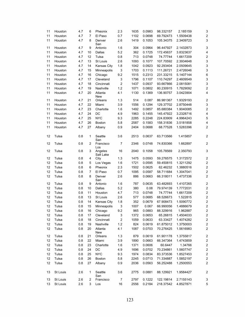
123

11 Houston 4.7 6 Pheonix 2.3 1635 0.0983 98.332157 2.185159 3 11 Houston 4.7 7 El Paso 0.7 1102 0.0698 69.792473 1.5509438 2 11 Houston 4.7 8 Denver 2.6 1419 0.1053 105.34375 2.3409723 3

11 Houston 4.7 9 San Antonio 1.6 304 0.0964 96.447927 2.1432873 3

11 Houston 4.7 10 Dallas 5.2 362 0.1725 172.45637 3.8323637 4 11 Houston 4.7 12 Tulsa 0.8 713 0.0748 74.77744 1.6617209 2 11 Houston 4.7 13 St Louis 2.6 1093 0.1077 107.70592 2.3934648 3 11 Houston 4.7 14 Kansas City 1.8 1042 0.0923 92.293404 2.0509645 3 11 Houston 4.7 15 Minneapolis 3 1703 0.1113 111.26721 2.4726046 3 11 Houston 4.7 16 Chicago 9.2 1515 0.2313 231.33215 5.1407144 6 11 Houston 4.7 17 Cleveland 3 1796 0.1107 110.74297 2.4609549 3 11 Houston 4.7 18 Cincinnati 2 1437 0.0937 93.667866 2.0815081 3 11 Houston 4.7 19 Nashville 1.2 1071 0.0802 80.230915 1.7829092 2 11 Houston 4.7 20 Atlanta 4.1 1130 0.1369 136.90757 3.0423904 4

11 Houston 4.7 21 New Orleans 1.3 514 0.087 86.981367 1.9329193 2

11 Houston 4.7 22 Miami 3.9 1556 0.1294 129.37702 2.8750448 3 11 Houston 4.7 23 Charlotte 1.6 1492 0.0857 85.680384 1.9040085 2 11 Houston 4.7 24 DC 4.9 1963 0.1455 145.47922 3.2328716 4 11 Houston 4.7 25 NYC 9.3 2285 0.2248 224.83909 4.9964243 5 11 Houston 4.7 26 Boston 5.8 2587 0.1583 158.31836 3.5181858 4 11 Houston 4.7 27 Albany 0.9 2404 0.0688 68.77528 1.5283396 2

12 Tulsa 0.8 1 Seattle 3.6 2513 0.0637 63.713566 1.415857 2

12 Tulsa 0.8 2 San Francisco 7 2346 0.0748 74.830366 1.662897 2

12 Tulsa 0.8 3 Los Angeles 16 2040 0.1058 105.78569 2.350793 3

12 Tulsa 0.8 4 Salt Lake City 1.3 1475 0.0593 59.276575 1.3172572 2

12 Tulsa 0.8 5 Los Vegas 1.6 1721 0.0595 59.450815 1.3211292 2 12 Tulsa 0.8 6 Pheonix 2.3 1502 0.0625 62.46232 1.3880516 2 12 Tulsa 0.8 7 El Paso 0.7 1095 0.0587 58.711684 1.3047041 2 12 Tulsa 0.8 8 Denver 2.6 886 0.0663 66.318011 1.4737336 2

12 Tulsa 0.8 9 San Antonio 1.6 787 0.0635 63.482693 1.4107265 2

12 Tulsa 0.8 10 Dallas 5.2 380 0.08 79.974139 1.7772031 2 12 Tulsa 0.8 11 Houston 4.7 713 0.0748 74.77744 1.6617209 2 12 Tulsa 0.8 13 St Louis 2.6 577 0.0685 68.526673 1.522815 2 12 Tulsa 0.8 14 Kansas City 1.8 352 0.0679 67.908473 1.5090772 2 12 Tulsa 0.8 15 Minneapolis 3 1007 0.067 66.990056 1.4886679 2 12 Tulsa 0.8 16 Chicago 9.2 965 0.0883 88.329916 1.962887 2 12 Tulsa 0.8 17 Cleveland 3 1372 0.0653 65.26815 1.4504033 2 12 Tulsa 0.8 18 Cincinnati 2 1059 0.0633 63.33427 1.4074282 2 12 Tulsa 0.8 19 Nashville 1.2 824 0.0619 61.875012 1.3750003 2 12 Tulsa 0.8 20 Atlanta 4.1 1087 0.0703 70.276425 1.5616983 2

12 Tulsa 0.8 21 New Orleans 1.3 879 0.0619 61.901178 1.3755817 2

12 Tulsa 0.8 22 Miami 3.9 1890 0.0663 66.347364 1.4743859 2 12 Tulsa 0.8 23 Charlotte 1.6 1371 0.0606 60.6447 1.34766 2 12 Tulsa 0.8 24 DC 4.9 1696 0.0702 70.234861 1.5607747 2 12 Tulsa 0.8 25 NYC 9.3 1974 0.0834 83.373536 1.8527453 2 12 Tulsa 0.8 26 Boston 5.8 2245 0.0713 71.334887 1.5852197 2 12 Tulsa 0.8 27 Albany 0.9 2036 0.0563 56.252488 1.2500553 2

13 St Louis 2.6 1 Seattle 3.6 2775 0.0881 88.129921 1.9584427 2

13 St Louis 2.6 2 San Francisco 7 2797 0.1222 122.19814 2.7155143 3

13 St Louis 2.6 3 Los 16 2556 0.2184 218.37542 4.8527871 5

124

Angeles

13 St Louis 2.6 4 Salt Lake City 1.3 1866 0.0674 67.418067 1.4981793 2

13 St Louis 2.6 5 Los Vegas 1.6 2218 0.0695 69.451589 1.5433686 2 13 St Louis 2.6 6 Pheonix 2.3 2046 0.0772 77.192925 1.7153983 2 13 St Louis 2.6 7 El Paso 0.7 1669 0.0616 61.567612 1.3681692 2 13 St Louis 2.6 8 Denver 2.6 1278 0.0837 83.684796 1.8596621 2

13 St Louis 2.6 9 San Antonio 1.6 1278 0.0729 72.91775 1.6203944 2

13 St Louis 2.6 10 Dallas 5.2 879 0.1152 115.192 2.5598223 3 13 St Louis 2.6 11 Houston 4.7 1093 0.1077 107.70592 2.3934648 3 13 St Louis 2.6 12 Tulsa 0.8 577 0.0685 68.526673 1.522815 2 13 St Louis 2.6 14 Kansas City 1.8 384 0.0822 82.208423 1.8268538 2 13 St Louis 2.6 15 Minneapolis 3 754 0.0919 91.861813 2.0413736 3 13 St Louis 2.6 16 Chicago 9.2 427 0.1683 168.29841 3.7399647 4 13 St Louis 2.6 17 Cleveland 3 796 0.0915 91.474853 2.0327745 3 13 St Louis 2.6 18 Cincinnati 2 496 0.0831 83.140417 1.8475648 2 13 St Louis 2.6 19 Nashville 1.2 407 0.0749 74.853776 1.6634172 2 13 St Louis 2.6 20 Atlanta 4.1 755 0.1042 104.2158 2.3159067 3

13 St Louis 2.6 21 New Orleans 1.3 963 0.0714 71.352249 1.5856055 2

13 St Louis 2.6 22 Miami 3.9 1710 0.0952 95.238039 2.1164009 3 13 St Louis 2.6 23 Charlotte 1.6 915 0.075 74.969381 1.6659862 2 13 St Louis 2.6 24 DC 4.9 1145 0.1095 109.46195 2.4324878 3 13 St Louis 2.6 25 NYC 9.3 1405 0.1546 154.56118 3.434693 4 13 St Louis 2.6 26 Boston 5.8 1673 0.1154 115.40677 2.5645948 3 13 St Louis 2.6 27 Albany 0.9 1458 0.0644 64.387676 1.4308372 2

14 Kansas City 1.8 1 Seattle 3.6 2423 0.078 77.970382 1.7326752 2

14 Kansas City 1.8 2 San Francisco 7 2417 0.1019 101.93869 2.2653041 3

14 Kansas City 1.8 3 Los Angeles 16 2187 0.1697 169.69656 3.7710346 4

14 Kansas City 1.8 4 Salt Lake City 1.3 1487 0.0645 64.532506 1.4340557 2

14 Kansas City 1.8 5 Los Vegas 1.6 1840 0.0655 65.497009 1.4554891 2 14 Kansas City 1.8 6 Pheonix 2.3 1687 0.0711 71.097842 1.579952 2 14 Kansas City 1.8 7 El Paso 0.7 1357 0.0604 60.447828 1.3432851 2 14 Kansas City 1.8 8 Denver 2.6 898 0.0773 77.299936 1.7177764 2

14 Kansas City 1.8 9 San Antonio 1.6 1139 0.0683 68.278687 1.5173041 2

14 Kansas City 1.8 10 Dallas 5.2 732 0.0988 98.831698 2.1962599 3 14 Kansas City 1.8 11 Houston 4.7 1042 0.0923 92.293404 2.0509645 3 14 Kansas City 1.8 12 Tulsa 0.8 352 0.0679 67.908473 1.5090772 2 14 Kansas City 1.8 13 St Louis 2.6 384 0.0822 82.208423 1.8268538 2 14 Kansas City 1.8 15 Minneapolis 3 660 0.0823 82.31697 1.829266 2 14 Kansas City 1.8 16 Chicago 9.2 664 0.131 130.99787 2.9110637 3 14 Kansas City 1.8 17 Cleveland 3 1129 0.0789 78.874781 1.7527729 2 14 Kansas City 1.8 18 Cincinnati 2 869 0.0729 72.885975 1.6196883 2 14 Kansas City 1.8 19 Nashville 1.2 763 0.0674 67.416282 1.4981396 2 14 Kansas City 1.8 20 Atlanta 4.1 1090 0.0874 87.416705 1.9425934 2

14 Kansas City 1.8 21 New Orleans 1.3 1099 0.0662 66.218091 1.4715131 2

14 Kansas City 1.8 22 Miami 3.9 2001 0.0815 81.488421 1.8108538 2 14 Kansas City 1.8 23 Charlotte 1.6 1292 0.0676 67.554183 1.5012041 2 14 Kansas City 1.8 24 DC 4.9 1520 0.0908 90.845015 2.0187781 3 14 Kansas City 1.8 25 NYC 9.3 1764 0.1216 121.55009 2.7011132 3 14 Kansas City 1.8 26 Boston 5.8 2012 0.0951 95.057357 2.1123857 3 14 Kansas City 1.8 27 Albany 0.9 1791 0.0604 60.414702 1.3425489 2

125

15 Minneapolis 3 1 Seattle 3.6 2248 0.0955 95.52498 2.1227773 3

15 Minneapolis 3 2 San Francisco 7 2552 0.1341 134.14066 2.9809035 3

15 Minneapolis 3 3 Los Angeles 16 2461 0.2448 244.7672 5.4392711 6

15 Minneapolis 3 4 Salt Lake City 1.3 1585 0.0705 70.514202 1.5669823 2

15 Minneapolis 3 5 Los Vegas 1.6 2085 0.0724 72.380837 1.6084631 2 15 Minneapolis 3 6 Pheonix 2.3 2055 0.0808 80.816305 1.7959179 2 15 Minneapolis 3 7 El Paso 0.7 1864 0.0621 62.055573 1.3790127 2 15 Minneapolis 3 8 Denver 2.6 1122 0.089 88.964528 1.9769895 2

15 Minneapolis 3 9 San Antonio 1.6 1791 0.0734 73.375186 1.6305597 2

15 Minneapolis 3 10 Dallas 5.2 1390 0.1194 119.42858 2.6539684 3 15 Minneapolis 3 11 Houston 4.7 1703 0.1113 111.26721 2.4726046 3 15 Minneapolis 3 12 Tulsa 0.8 1007 0.067 66.990056 1.4886679 2 15 Minneapolis 3 13 St Louis 2.6 754 0.0919 91.861813 2.0413736 3 15 Minneapolis 3 14 Kansas City 1.8 660 0.0823 82.31697 1.829266 2 15 Minneapolis 3 16 Chicago 9.2 572 0.1812 181.1721 4.0260466 5 15 Minneapolis 3 17 Cleveland 3 1017 0.0948 94.757693 2.1057265 3 15 Minneapolis 3 18 Cincinnati 2 972 0.0824 82.398819 1.8310849 2 15 Minneapolis 3 19 Nashville 1.2 1124 0.0714 71.368667 1.5859704 2 15 Minneapolis 3 20 Atlanta 4.1 1463 0.1054 105.39253 2.3420561 3

15 Minneapolis 3 21 New Orleans 1.3 1695 0.0701 70.098315 1.5577403 2

15 Minneapolis 3 22 Miami 3.9 2436 0.0983 98.345913 2.1854647 3 15 Minneapolis 3 23 Charlotte 1.6 1513 0.0745 74.47495 1.6549989 2 15 Minneapolis 3 24 DC 4.9 1504 0.1149 114.93932 2.554207 3 15 Minneapolis 3 25 NYC 9.3 1637 0.1676 167.59007 3.7242238 4 15 Minneapolis 3 26 Boston 5.8 1808 0.1239 123.9354 2.7541201 3 15 Minneapolis 3 27 Albany 0.9 1584 0.0653 65.34754 1.4521676 2

16 Chicago 9.2 1 Seattle 3.6 2794 0.1798 179.82461 3.9961025 4

16 Chicago 9.2 2 San Francisco 7 2980 0.2988 298.81914 6.6404253 7

16 Chicago 9.2 3 Los Angeles 16 2807 0.6343 634.28757 14.095279 15

16 Chicago 9.2 4 Salt Lake City 1.3 2025 0.101 101.04719 2.245493 3

16 Chicago 9.2 5 Los Vegas 1.6 2453 0.1101 110.08593 2.4463539 3 16 Chicago 9.2 6 Pheonix 2.3 2340 0.1358 135.84014 3.0186698 4 16 Chicago 9.2 7 El Paso 0.7 2025 0.0784 78.362474 1.7413883 2 16 Chicago 9.2 8 Denver 2.6 1479 0.1528 152.81123 3.3958051 4

16 Chicago 9.2 9 San Antonio 1.6 1700 0.1138 113.78917 2.5286483 3

16 Chicago 9.2 10 Dallas 5.2 1296 0.2535 253.50117 5.6333594 6 16 Chicago 9.2 11 Houston 4.7 1515 0.2313 231.33215 5.1407144 6 16 Chicago 9.2 12 Tulsa 0.8 965 0.0883 88.329916 1.962887 2 16 Chicago 9.2 13 St Louis 2.6 427 0.1683 168.29841 3.7399647 4 16 Chicago 9.2 14 Kansas City 1.8 664 0.131 130.99787 2.9110637 3 16 Chicago 9.2 15 Minneapolis 3 572 0.1812 181.1721 4.0260466 5 16 Chicago 9.2 17 Cleveland 3 496 0.183 183.00879 4.0668619 5 16 Chicago 9.2 18 Cincinnati 2 407 0.1439 143.8884 3.1975201 4 16 Chicago 9.2 19 Nashville 1.2 643 0.1072 107.15798 2.3812884 3 16 Chicago 9.2 20 Atlanta 4.1 948 0.2172 217.23397 4.8274216 5

16 Chicago 9.2 21 New Orleans 1.3 1344 0.1048 104.76623 2.3281386 3

16 Chicago 9.2 22 Miami 3.9 1918 0.1971 197.13694 4.3808209 5 16 Chicago 9.2 23 Charlotte 1.6 949 0.1196 119.57714 2.6572697 3 16 Chicago 9.2 24 DC 4.9 960 0.2482 248.22705 5.5161567 6 16 Chicago 9.2 25 NYC 9.3 1145 0.4138 413.83875 9.1964166 10

126

16 Chicago 9.2 26 Boston 5.8 1367 0.2751 275.07134 6.1126965 7 16 Chicago 9.2 27 Albany 0.9 1145 0.0899 89.896904 1.997709 2

17 Cleveland 3 1 Seattle 3.6 3260 0.0923 92.298376 2.051075 3

17 Cleveland 3 2 San Francisco 7 3480 0.1303 130.32267 2.8960594 3

17 Cleveland 3 3 Los Angeles 16 3302 0.2382 238.17948 5.2928774 6

17 Cleveland 3 4 Salt Lake City 1.3 2522 0.0676 67.626731 1.5028162 2

17 Cleveland 3 5 Los Vegas 1.6 2945 0.0701 70.121926 1.558265 2 17 Cleveland 3 6 Pheonix 2.3 2815 0.0785 78.520261 1.7448947 2 17 Cleveland 3 7 El Paso 0.7 2465 0.0605 60.502957 1.3445102 2 17 Cleveland 3 8 Denver 2.6 1975 0.0847 84.693471 1.8820771 2

17 Cleveland 3 9 San Antonio 1.6 2027 0.0726 72.565525 1.6125672 2

17 Cleveland 3 10 Dallas 5.2 1650 0.1177 117.6541 2.6145355 3 17 Cleveland 3 11 Houston 4.7 1796 0.1107 110.74297 2.4609549 3 17 Cleveland 3 12 Tulsa 0.8 1372 0.0653 65.26815 1.4504033 2 17 Cleveland 3 13 St Louis 2.6 796 0.0915 91.474853 2.0327745 3 17 Cleveland 3 14 Kansas City 1.8 1129 0.0789 78.874781 1.7527729 2 17 Cleveland 3 15 Minneapolis 3 1017 0.0948 94.757693 2.1057265 3 17 Cleveland 3 16 Chicago 9.2 496 0.183 183.00879 4.0668619 5 17 Cleveland 3 18 Cincinnati 2 358 0.0886 88.583321 1.9685182 2 17 Cleveland 3 19 Nashville 1.2 741 0.0738 73.802978 1.6400662 2 17 Cleveland 3 20 Atlanta 4.1 894 0.1098 109.83187 2.4407083 3

17 Cleveland 3 21 New Orleans 1.3 1489 0.0709 70.90061 1.5755691 2

17 Cleveland 3 22 Miami 3.9 1769 0.1012 101.23137 2.2495859 3 17 Cleveland 3 23 Charlotte 1.6 706 0.0793 79.291529 1.762034 2 17 Cleveland 3 24 DC 4.9 492 0.1256 125.56562 2.7903472 3 17 Cleveland 3 25 NYC 9.3 649 0.1808 180.811 4.0180222 5 17 Cleveland 3 26 Boston 5.8 884 0.1317 131.70537 2.926786 3 17 Cleveland 3 27 Albany 0.9 668 0.0701 70.147003 1.5588223 2

18 Cincinnati 2 1 Seattle 3.6 3174 0.0788 78.792129 1.7509362 2

18 Cincinnati 2 2 San Francisco 7 3280 0.1044 104.41911 2.3204246 3

18 Cincinnati 2 3 Los Angeles 16 3048 0.1771 177.14983 3.9366628 4

18 Cincinnati 2 4 Salt Lake City 1.3 2333 0.063 63.007383 1.4001641 2

18 Cincinnati 2 5 Los Vegas 1.6 2708 0.0645 64.473431 1.4327429 2 18 Cincinnati 2 6 Pheonix 2.3 2540 0.0703 70.309484 1.562433 2 18 Cincinnati 2 7 El Paso 0.7 2158 0.0586 58.553209 1.3011824 2 18 Cincinnati 2 8 Denver 2.6 1759 0.0751 75.103953 1.6689767 2

18 Cincinnati 2 9 San Antonio 1.6 1674 0.0673 67.344027 1.4965339 2

18 Cincinnati 2 10 Dallas 5.2 1308 0.0986 98.563041 2.1902898 3 18 Cincinnati 2 11 Houston 4.7 1437 0.0937 93.667866 2.0815081 3 18 Cincinnati 2 12 Tulsa 0.8 1059 0.0633 63.33427 1.4074282 2 18 Cincinnati 2 13 St Louis 2.6 496 0.0831 83.140417 1.8475648 2 18 Cincinnati 2 14 Kansas City 1.8 869 0.0729 72.885975 1.6196883 2 18 Cincinnati 2 15 Minneapolis 3 972 0.0824 82.398819 1.8310849 2 18 Cincinnati 2 16 Chicago 9.2 407 0.1439 143.8884 3.1975201 4 18 Cincinnati 2 17 Cleveland 3 358 0.0886 88.583321 1.9685182 2 18 Cincinnati 2 19 Nashville 1.2 387 0.0718 71.833288 1.5962953 2 18 Cincinnati 2 20 Atlanta 4.1 600 0.0952 95.215665 2.1159037 3

18 Cincinnati 2 21 New Orleans 1.3 1131 0.0671 67.147442 1.4921654 2

18 Cincinnati 2 22 Miami 3.9 1537 0.0866 86.599566 1.9244348 2

127

18 Cincinnati 2 23 Charlotte 1.6 541 0.0738 73.772619 1.6393915 2 18 Cincinnati 2 24 DC 4.9 648 0.1017 101.67307 2.2594015 3 18 Cincinnati 2 25 NYC 9.3 912 0.1365 136.48652 3.0330338 4 18 Cincinnati 2 26 Boston 5.8 1190 0.1044 104.35791 2.3190647 3 18 Cincinnati 2 27 Albany 0.9 984 0.0643 64.336087 1.4296908 2

19 Nashville 1.2 1 Seattle 3.6 3178 0.0678 67.794153 1.5065367 2

19 Nashville 1.2 2 San Francisco 7 3153 0.0834 83.423052 1.8538456 2

19 Nashville 1.2 3 Los Angeles 16 2860 0.1276 127.6486 2.8366355 3

19 Nashville 1.2 4 Salt Lake City 1.3 2239 0.0591 59.145609 1.3143469 2

19 Nashville 1.2 5 Los Vegas 1.6 2540 0.0599 59.869024 1.3304228 2 19 Nashville 1.2 6 Pheonix 2.3 2325 0.0637 63.655546 1.4145677 2 19 Nashville 1.2 7 El Paso 0.7 1890 0.0571 57.080574 1.2684572 2 19 Nashville 1.2 8 Denver 2.6 1645 0.0671 67.1239 1.4916422 2

19 Nashville 1.2 9 San Antonio 1.6 1328 0.0634 63.432928 1.4096206 2

19 Nashville 1.2 10 Dallas 5.2 991 0.0833 83.283872 1.8507527 2 19 Nashville 1.2 11 Houston 4.7 1071 0.0802 80.230915 1.7829092 2 19 Nashville 1.2 12 Tulsa 0.8 824 0.0619 61.875012 1.3750003 2 19 Nashville 1.2 13 St Louis 2.6 407 0.0749 74.853776 1.6634172 2 19 Nashville 1.2 14 Kansas City 1.8 763 0.0674 67.416282 1.4981396 2 19 Nashville 1.2 15 Minneapolis 3 1124 0.0714 71.368667 1.5859704 2 19 Nashville 1.2 16 Chicago 9.2 643 0.1072 107.15798 2.3812884 3 19 Nashville 1.2 17 Cleveland 3 741 0.0738 73.802978 1.6400662 2 19 Nashville 1.2 18 Cincinnati 2 387 0.0718 71.833288 1.5962953 2 19 Nashville 1.2 20 Atlanta 4.1 345 0.0839 83.854553 1.8634345 2

19 Nashville 1.2 21 New Orleans 1.3 754 0.0649 64.884323 1.4418738 2

19 Nashville 1.2 22 Miami 3.9 1314 0.0749 74.893104 1.6642912 2 19 Nashville 1.2 23 Charlotte 1.6 550 0.068 68.02052 1.5115671 2 19 Nashville 1.2 24 DC 4.9 914 0.0823 82.299859 1.8288857 2 19 Nashville 1.2 25 NYC 9.3 1224 0.1023 102.28075 2.2729055 3 19 Nashville 1.2 26 Boston 5.8 1521 0.0833 83.252135 1.8500475 2 19 Nashville 1.2 27 Albany 0.9 1332 0.0598 59.831429 1.3295873 2

20 Atlanta 4.1 1 Seattle 3.6 3506 0.1066 106.64099 2.3697997 3

20 Atlanta 4.1 2 San Francisco 7 3435 0.1596 159.64832 3.5477404 4

20 Atlanta 4.1 3 Los Angeles 16 3120 0.3084 308.39712 6.8532693 7

20 Atlanta 4.1 4 Salt Lake City 1.3 2545 0.0731 73.140101 1.6253356 2

20 Atlanta 4.1 5 Los Vegas 1.6 2807 0.0772 77.228626 1.7161917 2 20 Atlanta 4.1 6 Pheonix 2.3 2560 0.0891 89.06136 1.9791413 2 20 Atlanta 4.1 7 El Paso 0.7 2086 0.0644 64.39743 1.431054 2 20 Atlanta 4.1 8 Denver 2.6 1949 0.0962 96.207855 2.1379523 3

20 Atlanta 4.1 9 San Antonio 1.6 1421 0.0821 82.104599 1.8245466 2

20 Atlanta 4.1 10 Dallas 5.2 1158 0.1452 145.18741 3.2263868 4 20 Atlanta 4.1 11 Houston 4.7 1130 0.1369 136.90757 3.0423904 4 20 Atlanta 4.1 12 Tulsa 0.8 1087 0.0703 70.276425 1.5616983 2 20 Atlanta 4.1 13 St Louis 2.6 755 0.1042 104.2158 2.3159067 3 20 Atlanta 4.1 14 Kansas City 1.8 1090 0.0874 87.416705 1.9425934 2 20 Atlanta 4.1 15 Minneapolis 3 1463 0.1054 105.39253 2.3420561 3 20 Atlanta 4.1 16 Chicago 9.2 948 0.2172 217.23397 4.8274216 5 20 Atlanta 4.1 17 Cleveland 3 894 0.1098 109.83187 2.4407083 3 20 Atlanta 4.1 18 Cincinnati 2 600 0.0952 95.215665 2.1159037 3

128

20 Atlanta 4.1 19 Nashville 1.2 345 0.0839 83.854553 1.8634345 2

20 Atlanta 4.1 21 New Orleans 1.3 680 0.0818 81.827177 1.8183817 2

20 Atlanta 4.1 22 Miami 3.9 975 0.1247 124.69389 2.7709754 3 20 Atlanta 4.1 23 Charlotte 1.6 364 0.091 91.040004 2.0231112 3 20 Atlanta 4.1 24 DC 4.9 875 0.1433 143.30756 3.1846124 4 20 Atlanta 4.1 25 NYC 9.3 1205 0.2147 214.66304 4.7702897 5 20 Atlanta 4.1 26 Boston 5.8 1510 0.152 151.96371 3.3769714 4 20 Atlanta 4.1 27 Albany 0.9 1358 0.0702 70.19776 1.5599502 2

21 New Orleans 1.3 1 Seattle 3.6 3384 0.0688 68.761844 1.528041 2

21 New Orleans 1.3 2

San Francisco 7 3088 0.0863 86.263579 1.9169684 2

21 New Orleans 1.3 3

Los Angeles 16 2686 0.1347 134.74913 2.9944251 3

21 New Orleans 1.3 4

Salt Lake City 1.3 2306 0.0595 59.497779 1.3221729 2

21 New Orleans 1.3 5 Los Vegas 1.6 2434 0.0607 60.729695 1.3495488 2

21 New Orleans 1.3 6 Pheonix 2.3 2116 0.0651 65.114415 1.446987 2

21 New Orleans 1.3 7 El Paso 0.7 1595 0.0582 58.222929 1.2938429 2

21 New Orleans 1.3 8 Denver 2.6 1741 0.0678 67.835938 1.5074653 2

21 New Orleans 1.3 9

San Antonio 1.6 818 0.0667 66.706616 1.4823692 2

21 New Orleans 1.3 10 Dallas 5.2 710 0.0878 87.770319 1.9504515 2

21 New Orleans 1.3 11 Houston 4.7 514 0.087 86.981367 1.9329193 2

21 New Orleans 1.3 12 Tulsa 0.8 879 0.0619 61.901178 1.3755817 2

21 New Orleans 1.3 13 St Louis 2.6 963 0.0714 71.352249 1.5856055 2

21 New Orleans 1.3 14 Kansas City 1.8 1099 0.0662 66.218091 1.4715131 2

21 New Orleans 1.3 15 Minneapolis 3 1695 0.0701 70.098315 1.5577403 2

21 New Orleans 1.3 16 Chicago 9.2 1344 0.1048 104.76623 2.3281386 3

21 New Orleans 1.3 17 Cleveland 3 1489 0.0709 70.90061 1.5755691 2

21 New Orleans 1.3 18 Cincinnati 2 1131 0.0671 67.147442 1.4921654 2

21 New Orleans 1.3 19 Nashville 1.2 754 0.0649 64.884323 1.4418738 2

21 New Orleans 1.3 20 Atlanta 4.1 680 0.0818 81.827177 1.8183817 2

21 New Orleans 1.3 22 Miami 3.9 1076 0.0778 77.805005 1.7290001 2

21 New Orleans 1.3 23 Charlotte 1.6 1045 0.0654 65.400391 1.453342 2

21 New Orleans 1.3 24 DC 4.9 1553 0.0807 80.698193 1.7932932 2

21 New Orleans 1.3 25 NYC 9.3 1882 0.1022 102.23482 2.271885 3

21 New Orleans 1.3 26 Boston 5.8 2188 0.0829 82.885948 1.84191 2

21 New Orleans 1.3 27 Albany 0.9 2027 0.058 58.006291 1.2890287 2

22 Miami 3.9 1 Seattle 3.6 4402 0.1017 101.70364 2.260081 3

22 Miami 3.9 2 San Francisco 7 4165 0.1516 151.56037 3.3680082 4

22 Miami 3.9 3 Los Angeles 16 2760 0.2993 299.25407 6.6500905 7

129

22 Miami 3.9 4 Salt Lake City 1.3 3358 0.0703 70.292039 1.5620453 2

22 Miami 3.9 5 Los Vegas 1.6 3508 0.0744 74.426938 1.653932 2 22 Miami 3.9 6 Pheonix 2.3 3189 0.0855 85.508679 1.9001929 2 22 Miami 3.9 7 El Paso 0.7 2660 0.0625 62.454312 1.3878736 2 22 Miami 3.9 8 Denver 2.6 2777 0.0911 91.13775 2.0252833 3

22 Miami 3.9 9 San Antonio 1.6 1848 0.0789 78.944478 1.7543217 2

22 Miami 3.9 10 Dallas 5.2 1785 0.1357 135.66077 3.0146839 4 22 Miami 3.9 11 Houston 4.7 1556 0.1294 129.37702 2.8750448 3 22 Miami 3.9 12 Tulsa 0.8 1890 0.0663 66.347364 1.4743859 2 22 Miami 3.9 13 St Louis 2.6 1710 0.0952 95.238039 2.1164009 3 22 Miami 3.9 14 Kansas City 1.8 2001 0.0815 81.488421 1.8108538 2 22 Miami 3.9 15 Minneapolis 3 2436 0.0983 98.345913 2.1854647 3 22 Miami 3.9 16 Chicago 9.2 1918 0.1971 197.13694 4.3808209 5 22 Miami 3.9 17 Cleveland 3 1769 0.1012 101.23137 2.2495859 3 22 Miami 3.9 18 Cincinnati 2 1537 0.0866 86.599566 1.9244348 2 22 Miami 3.9 19 Nashville 1.2 1314 0.0749 74.893104 1.6642912 2 22 Miami 3.9 20 Atlanta 4.1 975 0.1247 124.69389 2.7709754 3

22 Miami 3.9 21 New Orleans 1.3 1076 0.0778 77.805005 1.7290001 2

22 Miami 3.9 23 Charlotte 1.6 1051 0.0829 82.882136 1.8418253 2 22 Miami 3.9 24 DC 4.9 1488 0.1331 133.07108 2.9571352 3 22 Miami 3.9 25 NYC 9.3 1758 0.2002 200.24705 4.4499345 5 22 Miami 3.9 26 Boston 5.8 2025 0.1434 143.44182 3.1875961 4 22 Miami 3.9 27 Albany 0.9 1968 0.0672 67.242134 1.4942696 2

23 Charlotte 1.6 1 Seattle 3.6 3672 0.0723 72.300459 1.6066769 2

23 Charlotte 1.6 2 San Francisco 7 3696 0.0927 92.720041 2.0604454 3

23 Charlotte 1.6 3 Los Angeles 16 3410 0.1504 150.43354 3.3429675 4

23 Charlotte 1.6 4 Salt Lake City 1.3 2776 0.06 59.998059 1.3332902 2

23 Charlotte 1.6 5 Los Vegas 1.6 3090 0.0612 61.239308 1.3608735 2 23 Charlotte 1.6 6 Pheonix 2.3 2868 0.066 65.980382 1.4662307 2 23 Charlotte 1.6 7 El Paso 0.7 2416 0.0569 56.888703 1.2641934 2 23 Charlotte 1.6 8 Denver 2.6 2184 0.0695 69.549191 1.5455376 2

23 Charlotte 1.6 9 San Antonio 1.6 1782 0.0644 64.397025 1.431045 2

23 Charlotte 1.6 10 Dallas 5.2 1495 0.0889 88.933809 1.9763069 2 23 Charlotte 1.6 11 Houston 4.7 1492 0.0857 85.680384 1.9040085 2 23 Charlotte 1.6 12 Tulsa 0.8 1371 0.0606 60.6447 1.34766 2 23 Charlotte 1.6 13 St Louis 2.6 915 0.075 74.969381 1.6659862 2 23 Charlotte 1.6 14 Kansas City 1.8 1292 0.0676 67.554183 1.5012041 2 23 Charlotte 1.6 15 Minneapolis 3 1513 0.0745 74.47495 1.6549989 2 23 Charlotte 1.6 16 Chicago 9.2 949 0.1196 119.57714 2.6572697 3 23 Charlotte 1.6 17 Cleveland 3 706 0.0793 79.291529 1.762034 2 23 Charlotte 1.6 18 Cincinnati 2 541 0.0738 73.772619 1.6393915 2 23 Charlotte 1.6 19 Nashville 1.2 550 0.068 68.02052 1.5115671 2 23 Charlotte 1.6 20 Atlanta 4.1 364 0.091 91.040004 2.0231112 3

23 Charlotte 1.6 21 New Orleans 1.3 1045 0.0654 65.400391 1.453342 2

23 Charlotte 1.6 22 Miami 3.9 1051 0.0829 82.882136 1.8418253 2 23 Charlotte 1.6 24 DC 4.9 329 0.0975 97.464627 2.1658806 3 23 Charlotte 1.6 25 NYC 9.3 857 0.1212 121.24606 2.6943568 3 23 Charlotte 1.6 26 Boston 5.8 1160 0.0949 94.895905 2.1087979 3 23 Charlotte 1.6 27 Albany 0.9 1029 0.0626 62.62278 1.3916173 2

24 DC 4.9 1 Seattle 3.6 3742 0.1168 116.80933 2.595763 3

130

24 DC 4.9 2 San Francisco 7 3918 0.1786 178.62918 3.9695372 4

24 DC 4.9 3 Los Angeles 16 3698 0.3529 352.86585 7.8414634 8

24 DC 4.9 4 Salt Lake City 1.3 2970 0.0761 76.095102 1.6910023 2

24 DC 4.9 5 Los Vegas 1.6 3355 0.0808 80.813395 1.7958532 2 24 DC 4.9 6 Pheonix 2.3 3190 0.0943 94.278774 2.0950839 3 24 DC 4.9 7 El Paso 0.7 2788 0.0648 64.809704 1.4402156 2 24 DC 4.9 8 Denver 2.6 2400 0.1026 102.55288 2.2789528 3

24 DC 4.9 9 San Antonio 1.6 2235 0.0839 83.908363 1.8646303 2

24 DC 4.9 10 Dallas 5.2 1903 0.1557 155.68342 3.4596315 4 24 DC 4.9 11 Houston 4.7 1963 0.1455 145.47922 3.2328716 4 24 DC 4.9 12 Tulsa 0.8 1696 0.0702 70.234861 1.5607747 2 24 DC 4.9 13 St Louis 2.6 1145 0.1095 109.46195 2.4324878 3 24 DC 4.9 14 Kansas City 1.8 1520 0.0908 90.845015 2.0187781 3 24 DC 4.9 15 Minneapolis 3 1504 0.1149 114.93932 2.554207 3 24 DC 4.9 16 Chicago 9.2 960 0.2482 248.22705 5.5161567 6 24 DC 4.9 17 Cleveland 3 492 0.1256 125.56562 2.7903472 3 24 DC 4.9 18 Cincinnati 2 648 0.1017 101.67307 2.2594015 3 24 DC 4.9 19 Nashville 1.2 914 0.0823 82.299859 1.8288857 2 24 DC 4.9 20 Atlanta 4.1 875 0.1433 143.30756 3.1846124 4

24 DC 4.9 21 New Orleans 1.3 1553 0.0807 80.698193 1.7932932 2

24 DC 4.9 22 Miami 3.9 1488 0.1331 133.07108 2.9571352 3 24 DC 4.9 23 Charlotte 1.6 329 0.0975 97.464627 2.1658806 3 24 DC 4.9 25 NYC 9.3 329 0.2702 270.20703 6.0046008 7 24 DC 4.9 26 Boston 5.8 635 0.1834 183.38248 4.0751661 5 24 DC 4.9 27 Albany 0.9 510 0.0789 78.940974 1.7542439 2

25 NYC 9.3 1 Seattle 3.6 3871 0.1758 175.76214 3.9058254 4

25 NYC 9.3 2 San Francisco 7 4127 0.2924 292.41017 6.4980038 7

25 NYC 9.3 3 Los Angeles 16 3942 0.6205 620.54091 13.789798 14

25 NYC 9.3 4 Salt Lake City 1.3 3168 0.0975 97.469462 2.165988 3

25 NYC 9.3 5 Los Vegas 1.6 3590 0.1069 106.85617 2.3745814 3 25 NYC 9.3 6 Pheonix 2.3 3447 0.1319 131.91623 2.9314719 3 25 NYC 9.3 7 El Paso 0.7 3071 0.0757 75.682209 1.6818269 2 25 NYC 9.3 8 Denver 2.6 2619 0.1462 146.17408 3.2483129 4

25 NYC 9.3 9 San Antonio 1.6 2549 0.1103 110.3213 2.4515844 3

25 NYC 9.3 10 Dallas 5.2 2205 0.2439 243.92091 5.4204647 6 25 NYC 9.3 11 Houston 4.7 2285 0.2248 224.83909 4.9964243 5 25 NYC 9.3 12 Tulsa 0.8 1974 0.0834 83.373536 1.8527453 2 25 NYC 9.3 13 St Louis 2.6 1405 0.1546 154.56118 3.434693 4 25 NYC 9.3 14 Kansas City 1.8 1764 0.1216 121.55009 2.7011132 3 25 NYC 9.3 15 Minneapolis 3 1637 0.1676 167.59007 3.7242238 4 25 NYC 9.3 16 Chicago 9.2 1145 0.4138 413.83875 9.1964166 10 25 NYC 9.3 17 Cleveland 3 649 0.1808 180.811 4.0180222 5 25 NYC 9.3 18 Cincinnati 2 912 0.1365 136.48652 3.0330338 4 25 NYC 9.3 19 Nashville 1.2 1224 0.1023 102.28075 2.2729055 3 25 NYC 9.3 20 Atlanta 4.1 1205 0.2147 214.66304 4.7702897 5

25 NYC 9.3 21 New Orleans 1.3 1882 0.1022 102.23482 2.271885 3

25 NYC 9.3 22 Miami 3.9 1758 0.2002 200.24705 4.4499345 5 25 NYC 9.3 23 Charlotte 1.6 857 0.1212 121.24606 2.6943568 4 25 NYC 9.3 24 DC 4.9 329 0.2702 270.20703 6.0046008 7 25 NYC 9.3 26 Boston 5.8 306 0.3099 309.8511 6.88558 7

131

25 NYC 9.3 27 Albany 0.9 216 0.1012 101.17376 2.2483058 3 26 Boston 5.8 1 Seattle 3.6 4008 0.1281 128.14784 2.8477297 3

26 Boston 5.8 2 San Francisco 7 4330 0.2003 200.28796 4.4508435 5

26 Boston 5.8 3 Los Angeles 16 4173 0.4037 403.74024 8.9720053 9

26 Boston 5.8 4 Salt Lake City 1.3 3371 0.0796 79.638966 1.7697548 2

26 Boston 5.8 5 Los Vegas 1.6 3818 0.0852 85.235561 1.8941236 2 26 Boston 5.8 6 Pheonix 2.3 3698 0.1008 100.76508 2.239224 3 26 Boston 5.8 7 El Paso 0.7 3340 0.0661 66.051185 1.4678041 2 26 Boston 5.8 8 Denver 2.6 2844 0.11 109.98117 2.444026 3

26 Boston 5.8 9 San Antonio 1.6 2845 0.0876 87.618147 1.9470699 2

26 Boston 5.8 10 Dallas 5.2 2495 0.1702 170.16291 3.7813979 4 26 Boston 5.8 11 Houston 4.7 2587 0.1583 158.31836 3.5181858 4 26 Boston 5.8 12 Tulsa 0.8 2245 0.0713 71.334887 1.5852197 2 26 Boston 5.8 13 St Louis 2.6 1673 0.1154 115.40677 2.5645948 3 26 Boston 5.8 14 Kansas City 1.8 2012 0.0951 95.057357 2.1123857 3 26 Boston 5.8 15 Minneapolis 3 1808 0.1239 123.9354 2.7541201 3 26 Boston 5.8 16 Chicago 9.2 1367 0.2751 275.07134 6.1126965 7 26 Boston 5.8 17 Cleveland 3 884 0.1317 131.70537 2.926786 3 26 Boston 5.8 18 Cincinnati 2 1190 0.1044 104.35791 2.3190647 3 26 Boston 5.8 19 Nashville 1.2 1521 0.0833 83.252135 1.8500475 2 26 Boston 5.8 20 Atlanta 4.1 1510 0.152 151.96371 3.3769714 4

26 Boston 5.8 21 New Orleans 1.3 2188 0.0829 82.885948 1.84191 2

26 Boston 5.8 22 Miami 3.9 2025 0.1434 143.44182 3.1875961 4 26 Boston 5.8 23 Charlotte 1.6 1160 0.0949 94.895905 2.1087979 3 26 Boston 5.8 24 DC 4.9 635 0.1834 183.38248 4.0751661 5 26 Boston 5.8 25 NYC 9.3 306 0.3099 309.8511 6.88558 7 26 Boston 5.8 27 Albany 0.9 225 0.0866 86.6321 1.9251578 2

27 Albany 0.88 1 Seattle 3.6 3793 0.0623 62.298739 1.3844164 2

27 Albany 0.88 2 San Francisco 7 4110 0.0729 72.918916 1.6204204 2

27 Albany 0.88 3 Los Angeles 16 3952 0.104 103.97084 2.310463 3

27 Albany 0.88 4 Salt Lake City 1.3 3146 0.0557 55.708907 1.2379757 2

27 Albany 0.88 5 Los Vegas 1.6 3594 0.056 56.00836 1.2446302 2 27 Albany 0.88 6 Pheonix 2.3 3478 0.0585 58.501578 1.3000351 2 27 Albany 0.88 7 El Paso 0.7 3130 0.0537 53.660221 1.1924494 2 27 Albany 0.88 8 Denver 2.6 2620 0.0611 61.087334 1.3574963 2

27 Albany 0.88 9 San Antonio 1.6 2655 0.0576 57.613833 1.2803074 2

27 Albany 0.88 10 Dallas 5.2 2293 0.0708 70.795563 1.5732347 2 27 Albany 0.88 11 Houston 4.7 2404 0.0688 68.77528 1.5283396 2 27 Albany 0.88 12 Tulsa 0.8 2036 0.0563 56.252488 1.2500553 2 27 Albany 0.88 13 St Louis 2.6 1458 0.0644 64.387676 1.4308372 2 27 Albany 0.88 14 Kansas City 1.8 1791 0.0604 60.414702 1.3425489 2 27 Albany 0.88 15 Minneapolis 3 1584 0.0653 65.34754 1.4521676 2 27 Albany 0.88 16 Chicago 9.2 1145 0.0899 89.896904 1.997709 2 27 Albany 0.88 17 Cleveland 3 668 0.0701 70.147003 1.5588223 2 27 Albany 0.88 18 Cincinnati 2 984 0.0643 64.336087 1.4296908 2 27 Albany 0.88 19 Nashville 1.2 1332 0.0598 59.831429 1.3295873 2 27 Albany 0.88 20 Atlanta 4.1 1358 0.0702 70.19776 1.5599502 2

27 Albany 0.88 21 New Orleans 1.3 2027 0.058 58.006291 1.2890287 2

27 Albany 0.88 22 Miami 3.9 1968 0.0672 67.242134 1.4942696 2

132

27 Albany 0.88 23 Charlotte 1.6 1029 0.0626 62.62278 1.3916173 2 27 Albany 0.88 24 DC 4.9 510 0.0789 78.940974 1.7542439 2 27 Albany 0.88 25 NYC 9.3 216 0.1012 101.17376 2.2483058 3 27 Albany 0.88 26 Boston 5.8 225 0.0866 86.6321 1.9251578 2

Pan-European Traffic Matrix I pop j pop I j dist (km) traf *1000

1 0.482 2 0.612 1 2 320 0.007017 7.016961 0.155932 11 0.482 3 7.1 1 3 465 0.079222 79.22225 1.760494 21 0.482 4 0.729 1 4 757 0.007822 7.821801 0.173818 11 0.482 5 1 1 5 770 0.010714 10.71414 0.238092 11 0.482 6 2.2 1 6 782 0.02354 23.54037 0.523119 11 0.482 7 0.21 1 7 1032 0.002194 2.193971 0.048755 11 0.482 8 2.8 1 8 1452 0.028373 28.37315 0.630514 11 0.482 9 1.5 1 9 1477 0.015176 15.17629 0.337251 11 0.482 10 0.415 1 10 1163 0.00429 4.290155 0.095337 11 0.482 11 0.36 1 11 1237 0.003701 3.701141 0.082248 11 0.482 12 0.252 1 12 1115 0.002615 2.614872 0.058108 11 0.482 13 1.7 1 13 1075 0.017697 17.69705 0.393268 11 0.482 14 0.644 1 14 1085 0.006699 6.698584 0.148857 11 0.482 15 1.2 1 15 1378 0.012218 12.21778 0.271506 11 0.482 16 1.3 1 16 1418 0.013202 13.20164 0.29337 11 0.482 17 2.7 1 17 1883 0.026714 26.71354 0.593634 11 0.482 18 0.868 1 18 1799 0.008624 8.624332 0.191652 11 0.482 19 0.772 1 19 2855 0.007345 7.344683 0.163215 11 0.482 20 1.6 1 20 2146 0.015638 15.6383 0.347518 11 0.482 21 1.8 1 21 1894 0.017799 17.79939 0.395542 11 0.482 22 1.5 1 22 1680 0.014998 14.99829 0.333295 11 0.482 23 1.2 1 23 1467 0.012149 12.14855 0.269968 11 0.482 24 1.6 1 24 1820 0.01588 15.88031 0.352896 11 0.482 25 3.4 1 25 1316 0.034761 34.76132 0.772474 11 0.482 26 0.499 1 26 1244 0.005128 5.1276 0.113947 11 0.482 27 0.505 1 27 1266 0.005181 5.181101 0.115136 11 0.482 28 0.744 1 28 1616 0.007466 7.465769 0.165906 1

#VALUE! 2 0.612 1 0.482 2 1 320 0.007017 7.016961 0.155932 12 0.612 3 7.1 2 3 559 0.099156 99.15582 2.203463 32 0.612 4 0.729 2 4 713 0.009981 9.981261 0.221806 12 0.612 5 1 2 5 798 0.013563 13.56285 0.301397 12 0.612 6 2.2 2 6 898 0.029539 29.53876 0.656417 12 0.612 7 0.21 2 7 1258 0.002737 2.737168 0.060826 12 0.612 8 2.8 2 8 1717 0.035476 35.4765 0.788367 12 0.612 9 1.5 2 9 1683 0.01904 19.04034 0.423119 12 0.612 10 0.415 2 10 1297 0.005394 5.394345 0.119874 12 0.612 11 0.36 2 11 1290 0.004682 4.681711 0.104038 12 0.612 12 0.252 2 12 1152 0.003311 3.310525 0.073567 12 0.612 13 1.7 2 13 948 0.022719 22.71868 0.50486 12 0.612 14 0.644 2 14 1077 0.008511 8.510813 0.189129 12 0.612 15 1.2 2 15 1383 0.015508 15.50795 0.344621 12 0.612 16 1.3 2 16 1492 0.016685 16.68485 0.370774 12 0.612 17 2.7 2 17 1972 0.033773 33.773 0.750511 12 0.612 18 0.868 2 18 1801 0.010949 10.94927 0.243317 12 0.612 19 0.772 2 19 2881 0.009318 9.317567 0.207057 1

133

2 0.612 20 1.6 2 20 2130 0.01987 19.87003 0.441556 12 0.612 21 1.8 2 21 1848 0.022652 22.65171 0.503371 12 0.612 22 1.5 2 22 1640 0.019086 19.08574 0.424128 12 0.612 23 1.2 2 23 1405 0.015486 15.48578 0.344129 12 0.612 24 1.6 2 24 1689 0.020303 20.30304 0.451179 12 0.612 25 3.4 2 25 1205 0.044487 44.48715 0.988603 12 0.612 26 0.499 2 26 1052 0.006608 6.608214 0.146849 12 0.612 27 0.505 2 27 992 0.006722 6.72218 0.149382 12 0.612 28 0.744 2 28 1378 0.009618 9.618084 0.213735 1

3 7.1 1 0.482 3 1 465 0.079222 79.22225 1.760494 23 7.1 2 0.612 3 2 559 0.099156 99.15582 2.203463 33 7.1 4 0.729 3 4 354 0.122255 122.2547 2.716772 33 7.1 5 1 3 5 319 0.168928 168.9284 3.753964 43 7.1 6 2.2 3 6 344 0.369693 369.6934 8.215409 93 7.1 7 0.21 3 7 743 0.033242 33.24221 0.738716 13 7.1 8 2.8 3 8 1265 0.423186 423.1855 9.404123 103 7.1 9 1.5 3 9 1144 0.228751 228.7512 5.08336 63 7.1 10 0.415 3 10 737 0.065738 65.73754 1.460834 23 7.1 11 0.36 3 11 775 0.056785 56.78505 1.26189 23 7.1 12 0.252 3 12 650 0.040335 40.33492 0.896332 13 7.1 13 1.7 3 13 721 0.26978 269.7803 5.995118 63 7.1 14 0.644 3 14 636 0.103262 103.2616 2.294703 33 7.1 15 1.2 3 15 919 0.186548 186.5483 4.145518 53 7.1 16 1.3 3 16 958 0.201367 201.3672 4.474826 53 7.1 17 2.7 3 17 1432 0.403527 403.5266 8.967258 93 7.1 18 0.868 3 18 1337 0.130535 130.5354 2.900786 33 7.1 19 0.772 3 19 2394 0.11001 110.0101 2.44467 33 7.1 20 1.6 3 20 1692 0.235503 235.5033 5.233406 63 7.1 21 1.8 3 21 1448 0.268746 268.7462 5.972137 63 7.1 22 1.5 3 22 1232 0.227244 227.2444 5.049876 63 7.1 23 1.2 3 23 1031 0.184689 184.689 4.1042 53 7.1 24 1.6 3 24 1446 0.238916 238.9155 5.309233 63 7.1 25 3.4 3 25 930 0.52801 528.0097 11.73355 123 7.1 26 0.499 3 26 953 0.077329 77.32917 1.718426 23 7.1 27 0.505 3 27 1152 0.076965 76.96524 1.710339 23 7.1 28 0.744 3 28 1431 0.111201 111.2011 2.471135 3

4 0.729 1 0.482 4 1 757 0.007822 7.821801 0.173818 14 0.729 2 0.612 4 2 713 0.009981 9.981261 0.221806 14 0.729 3 7.1 4 3 354 0.122255 122.2547 2.716772 34 0.729 5 1 4 5 174 0.018009 18.00881 0.400196 14 0.729 6 2.2 4 6 431 0.037341 37.34107 0.829801 14 0.729 7 0.21 4 7 928 0.003349 3.349133 0.074425 14 0.729 8 2.8 4 8 1481 0.042836 42.83571 0.951905 14 0.729 9 1.5 4 9 1242 0.023316 23.31567 0.518126 14 0.729 10 0.415 4 10 739 0.006748 6.748141 0.149959 14 0.729 11 0.36 4 11 614 0.005944 5.943843 0.132085 14 0.729 12 0.252 4 12 469 0.00425 4.249967 0.094444 14 0.729 13 1.7 4 13 369 0.029186 29.18553 0.648567 14 0.729 14 0.644 4 14 363 0.011069 11.06918 0.245982 14 0.729 15 1.2 4 15 669 0.019675 19.67452 0.437212 1

134

4 0.729 16 1.3 4 16 830 0.020932 20.93244 0.465165 14 0.729 17 2.7 4 17 1298 0.041802 41.80232 0.92894 14 0.729 18 0.868 4 18 1088 0.013652 13.65185 0.303374 14 0.729 19 0.772 4 19 2166 0.011402 11.40223 0.253383 14 0.729 20 1.6 4 20 1419 0.024573 24.57295 0.546066 14 0.729 21 1.8 4 21 1150 0.028172 28.17163 0.626036 14 0.729 22 1.5 4 22 936 0.023905 23.9046 0.531213 14 0.729 23 1.2 4 23 712 0.019573 19.57339 0.434964 14 0.729 24 1.6 4 24 1094 0.025152 25.15248 0.558944 14 0.729 25 3.4 4 25 577 0.056418 56.41791 1.253731 24 0.729 26 0.499 4 26 620 0.008232 8.232334 0.182941 14 0.729 27 0.505 4 27 914 0.008064 8.064461 0.17921 14 0.729 28 0.744 4 28 1125 0.011667 11.66701 0.259267 1

5 1 1 0.482 5 1 770 0.010714 10.71414 0.238092 15 1 2 0.612 5 2 798 0.013563 13.56285 0.301397 15 1 3 7.1 5 3 319 0.168928 168.9284 3.753964 45 1 4 0.729 5 4 174 0.018009 18.00881 0.400196 15 1 6 2.2 5 6 264 0.05301 53.01008 1.178002 25 1 7 0.21 5 7 761 0.004673 4.672606 0.103836 15 1 8 2.8 5 8 1315 0.059396 59.39612 1.319914 25 1 9 1.5 5 9 1065 0.032423 32.42305 0.720512 15 1 10 0.415 5 10 569 0.009457 9.456778 0.210151 15 1 11 0.36 5 11 491 0.008299 8.299058 0.184424 15 1 12 0.252 5 12 351 0.005956 5.955836 0.132352 15 1 13 1.7 5 13 491 0.03919 39.19 0.870889 15 1 14 0.644 5 14 315 0.015336 15.33582 0.340796 15 1 15 1.2 5 15 604 0.027214 27.21418 0.60476 15 1 16 1.3 5 16 696 0.029142 29.14204 0.647601 15 1 17 2.7 5 17 1174 0.05786 57.8599 1.285775 25 1 18 0.868 5 18 1024 0.018827 18.82698 0.418377 15 1 19 0.772 5 19 2091 0.015693 15.69263 0.348725 15 1 20 1.6 5 20 1367 0.033822 33.82199 0.7516 15 1 21 1.8 5 21 1130 0.038704 38.70445 0.860099 15 1 22 1.5 5 22 912 0.032865 32.86472 0.730327 15 1 23 1.2 5 23 719 0.026828 26.82778 0.596173 15 1 24 1.6 5 24 1095 0.0345 34.49993 0.766665 15 1 25 3.4 5 25 578 0.07738 77.3801 1.719558 25 1 26 0.499 5 26 621 0.011291 11.29116 0.250915 15 1 27 0.505 5 27 912 0.011064 11.06445 0.245877 15 1 28 0.744 5 28 1126 0.016003 16.00287 0.355619 1

6 2.2 1 0.482 6 1 782 0.02354 23.54037 0.523119 16 2.2 2 0.612 6 2 898 0.029539 29.53876 0.656417 16 2.2 3 7.1 6 3 344 0.369693 369.6934 8.215409 96 2.2 4 0.729 6 4 431 0.037341 37.34107 0.829801 16 2.2 5 1 6 5 264 0.05301 53.01008 1.178002 26 2.2 7 0.21 6 7 496 0.010642 10.64211 0.236491 16 2.2 8 2.8 6 8 1051 0.133306 133.3058 2.962352 36 2.2 9 1.5 6 9 831 0.072882 72.88167 1.619593 26 2.2 10 0.415 6 10 393 0.021403 21.40309 0.475624 16 2.2 11 0.36 6 11 487 0.018269 18.26947 0.405988 1

135

6 2.2 12 0.252 6 12 397 0.012987 12.98693 0.288598 16 2.2 13 1.7 6 13 749 0.083328 83.32803 1.851734 26 2.2 14 0.644 6 14 478 0.032729 32.72903 0.727312 16 2.2 15 1.2 6 15 685 0.059259 59.25881 1.316862 26 2.2 16 1.3 6 16 639 0.064565 64.56456 1.434768 26 2.2 17 2.7 6 17 1104 0.127988 127.9883 2.844185 36 2.2 18 0.868 6 18 1081 0.041222 41.22248 0.916055 16 2.2 19 0.772 6 19 2096 0.034516 34.51607 0.767024 16 2.2 20 1.6 6 20 1449 0.074016 74.0162 1.644805 26 2.2 21 1.8 6 21 1245 0.084417 84.41711 1.875936 26 2.2 22 1.5 6 22 1031 0.071534 71.53447 1.589655 26 2.2 23 1.2 6 23 884 0.057998 57.99754 1.288834 26 2.2 24 1.6 6 24 1370 0.074394 74.39363 1.653192 26 2.2 25 3.4 6 25 879 0.164407 164.4065 3.653478 46 2.2 26 0.499 6 26 1028 0.023803 23.80322 0.52896 16 2.2 27 0.505 6 27 1345 0.02352 23.51962 0.522658 16 2.2 28 0.744 6 28 1544 0.034219 34.21875 0.760417 1

7 0.21 1 0.482 7 1 1032 0.002194 2.193971 0.048755 17 0.21 2 0.612 7 2 1258 0.002737 2.737168 0.060826 17 0.21 3 7.1 7 3 743 0.033242 33.24221 0.738716 17 0.21 4 0.729 7 4 928 0.003349 3.349133 0.074425 17 0.21 5 1 7 5 761 0.004673 4.672606 0.103836 17 0.21 6 2.2 7 6 496 0.010642 10.64211 0.236491 17 0.21 8 1.5 7 8 556 0.007191 7.191256 0.159806 17 0.21 9 0.415 7 9 449 0.002023 2.022858 0.044952 17 0.21 10 0.36 7 10 436 0.001759 1.758662 0.039081 17 0.21 11 0.252 7 11 761 0.001177 1.177497 0.026167 17 0.21 12 1.7 7 12 758 0.007946 7.946067 0.176579 17 0.21 13 0.644 7 13 1236 0.002885 2.884847 0.064108 17 0.21 14 1.2 7 14 907 0.005524 5.523893 0.122753 17 0.21 15 1.3 7 15 1001 0.005933 5.933177 0.131848 17 0.21 16 2.7 7 16 771 0.012602 12.60218 0.280048 17 0.21 17 0.868 7 17 1107 0.003927 3.926618 0.087258 17 0.21 18 0.772 7 18 1297 0.003443 3.443307 0.076518 17 0.21 19 1.6 7 19 2159 0.00681 6.809512 0.151322 17 0.21 20 1.8 7 20 1658 0.007851 7.85095 0.174466 17 0.21 21 1.5 7 21 1538 0.006588 6.587699 0.146393 17 0.21 22 1.2 7 22 1346 0.005334 5.334424 0.118543 17 0.21 23 1.6 7 23 1267 0.007151 7.151417 0.15892 17 0.21 24 3.4 7 24 1783 0.01473 14.73045 0.327343 17 0.21 25 0.499 7 25 1332 0.00222 2.220326 0.049341 17 0.21 26 0.505 7 26 1520 0.00222 2.220246 0.049339 17 0.21 27 0.744 7 27 1839 0.003214 3.214149 0.071426 17 0.21 28 0.482 7 28 2039 0.002062 2.062372 0.04583 1

8 2.8 1 0.482 8 1 1452 0.028373 28.37315 0.630514 18 2.8 2 0.612 8 2 1717 0.035476 35.4765 0.788367 18 2.8 3 7.1 8 3 1265 0.423186 423.1855 9.404123 108 2.8 4 0.729 8 4 1481 0.042836 42.83571 0.951905 18 2.8 5 1 8 5 1315 0.059396 59.39612 1.319914 28 2.8 6 2.2 8 6 1051 0.133306 133.3058 2.962352 3

136

8 2.8 7 0.21 8 7 556 0.013424 13.42368 0.298304 18 2.8 9 1.5 8 9 503 0.096641 96.64126 2.147584 38 2.8 10 0.415 8 10 910 0.025464 25.46403 0.565867 18 2.8 11 0.36 8 11 1248 0.021483 21.48336 0.477408 18 2.8 12 0.252 8 12 1284 0.015 15 0.333333 18 2.8 13 1.7 8 13 1789 0.098172 98.17247 2.18161 38 2.8 14 0.644 8 14 1446 0.037924 37.92363 0.842747 18 2.8 15 1.2 8 15 1485 0.070494 70.49412 1.566536 28 2.8 16 1.3 8 16 1186 0.077933 77.93305 1.731846 28 2.8 17 2.7 8 17 1362 0.159862 159.8619 3.552486 38 2.8 18 0.868 8 18 1702 0.050357 50.35707 1.119046 28 2.8 19 0.772 8 19 2372 0.043422 43.42207 0.964935 18 2.8 20 1.6 8 20 2032 0.09131 91.30997 2.02911 38 2.8 21 1.8 8 21 1976 0.102992 102.9919 2.288709 38 2.8 22 1.5 8 22 1809 0.086534 86.53365 1.92297 28 2.8 23 1.2 8 23 1775 0.069349 69.3486 1.54108 28 2.8 24 1.6 8 24 2292 0.090285 90.28518 2.006337 38 2.8 25 3.4 8 25 1869 0.19555 195.5503 4.345563 48 2.8 26 0.499 8 26 2072 0.028425 28.42547 0.631677 18 2.8 27 0.505 8 27 2387 0.028387 28.38745 0.630832 18 2.8 28 0.744 8 28 2592 0.041498 41.49785 0.922175 1

9 1.5 1 0.482 9 1 1477 0.015176 15.17629 0.337251 19 1.5 2 0.612 9 2 1683 0.01904 19.04034 0.423119 19 1.5 3 7.1 9 3 1144 0.228751 228.7512 5.08336 69 1.5 4 0.729 9 4 1242 0.023316 23.31567 0.518126 19 1.5 5 1 9 5 1065 0.032423 32.42305 0.720512 19 1.5 6 2.2 9 6 831 0.072882 72.88167 1.619593 29 1.5 7 0.21 9 7 449 0.007312 7.311534 0.162479 19 1.5 8 2.8 9 8 503 0.096641 96.64126 2.147584 39 1.5 10 0.415 9 10 533 0.014259 14.25885 0.316863 19 1.5 11 0.36 9 11 838 0.011918 11.91756 0.264835 19 1.5 12 0.252 9 12 915 0.00828 8.27956 0.18399 19 1.5 13 1.7 9 13 1476 0.05353 53.52965 1.189548 29 1.5 14 0.644 9 14 1096 0.020828 20.82765 0.462837 19 1.5 15 1.2 9 15 1055 0.03894 38.93999 0.865333 19 1.5 16 1.3 9 16 728 0.04355 43.54994 0.967776 19 1.5 17 2.7 9 17 858 0.089202 89.20171 1.98226 29 1.5 18 0.868 9 18 1216 0.027814 27.81394 0.618088 19 1.5 19 0.772 9 19 1878 0.023776 23.77587 0.528353 19 1.5 20 1.6 9 20 1532 0.05021 50.20993 1.115776 29 1.5 21 1.8 9 21 1501 0.056592 56.59173 1.257594 29 1.5 22 1.5 9 22 1349 0.047619 47.61921 1.058205 29 1.5 23 1.2 9 23 1355 0.03808 38.08009 0.846224 19 1.5 24 1.6 9 24 1869 0.049298 49.2984 1.09552 29 1.5 25 3.4 9 25 1501 0.106895 106.8955 2.375455 39 1.5 26 0.499 9 26 1765 0.015457 15.45671 0.343483 19 1.5 27 0.505 9 27 2148 0.015359 15.35915 0.341315 19 1.5 28 0.744 9 28 2280 0.022502 22.50179 0.50004 1

10 0.415 1 0.482 10 1 1163 0.00429 4.290155 0.095337 110 0.415 2 0.612 10 2 1297 0.005394 5.394345 0.119874 1

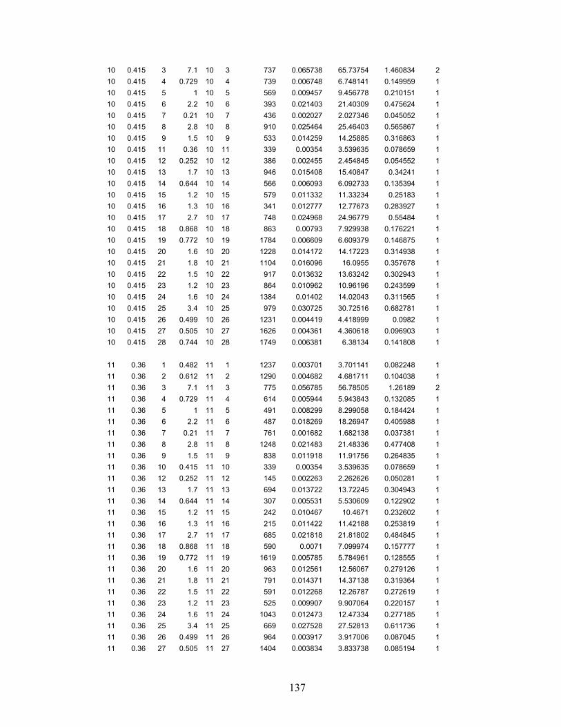
137

10 0.415 3 7.1 10 3 737 0.065738 65.73754 1.460834 210 0.415 4 0.729 10 4 739 0.006748 6.748141 0.149959 110 0.415 5 1 10 5 569 0.009457 9.456778 0.210151 110 0.415 6 2.2 10 6 393 0.021403 21.40309 0.475624 110 0.415 7 0.21 10 7 436 0.002027 2.027346 0.045052 110 0.415 8 2.8 10 8 910 0.025464 25.46403 0.565867 110 0.415 9 1.5 10 9 533 0.014259 14.25885 0.316863 110 0.415 11 0.36 10 11 339 0.00354 3.539635 0.078659 110 0.415 12 0.252 10 12 386 0.002455 2.454845 0.054552 110 0.415 13 1.7 10 13 946 0.015408 15.40847 0.34241 110 0.415 14 0.644 10 14 566 0.006093 6.092733 0.135394 110 0.415 15 1.2 10 15 579 0.011332 11.33234 0.25183 110 0.415 16 1.3 10 16 341 0.012777 12.77673 0.283927 110 0.415 17 2.7 10 17 748 0.024968 24.96779 0.55484 110 0.415 18 0.868 10 18 863 0.00793 7.929938 0.176221 110 0.415 19 0.772 10 19 1784 0.006609 6.609379 0.146875 110 0.415 20 1.6 10 20 1228 0.014172 14.17223 0.314938 110 0.415 21 1.8 10 21 1104 0.016096 16.0955 0.357678 110 0.415 22 1.5 10 22 917 0.013632 13.63242 0.302943 110 0.415 23 1.2 10 23 864 0.010962 10.96196 0.243599 110 0.415 24 1.6 10 24 1384 0.01402 14.02043 0.311565 110 0.415 25 3.4 10 25 979 0.030725 30.72516 0.682781 110 0.415 26 0.499 10 26 1231 0.004419 4.418999 0.0982 110 0.415 27 0.505 10 27 1626 0.004361 4.360618 0.096903 110 0.415 28 0.744 10 28 1749 0.006381 6.38134 0.141808 1

11 0.36 1 0.482 11 1 1237 0.003701 3.701141 0.082248 111 0.36 2 0.612 11 2 1290 0.004682 4.681711 0.104038 111 0.36 3 7.1 11 3 775 0.056785 56.78505 1.26189 211 0.36 4 0.729 11 4 614 0.005944 5.943843 0.132085 111 0.36 5 1 11 5 491 0.008299 8.299058 0.184424 111 0.36 6 2.2 11 6 487 0.018269 18.26947 0.405988 111 0.36 7 0.21 11 7 761 0.001682 1.682138 0.037381 111 0.36 8 2.8 11 8 1248 0.021483 21.48336 0.477408 111 0.36 9 1.5 11 9 838 0.011918 11.91756 0.264835 111 0.36 10 0.415 11 10 339 0.00354 3.539635 0.078659 111 0.36 12 0.252 11 12 145 0.002263 2.262626 0.050281 111 0.36 13 1.7 11 13 694 0.013722 13.72245 0.304943 111 0.36 14 0.644 11 14 307 0.005531 5.530609 0.122902 111 0.36 15 1.2 11 15 242 0.010467 10.4671 0.232602 111 0.36 16 1.3 11 16 215 0.011422 11.42188 0.253819 111 0.36 17 2.7 11 17 685 0.021818 21.81802 0.484845 111 0.36 18 0.868 11 18 590 0.0071 7.099974 0.157777 111 0.36 19 0.772 11 19 1619 0.005785 5.784961 0.128555 111 0.36 20 1.6 11 20 963 0.012561 12.56067 0.279126 111 0.36 21 1.8 11 21 791 0.014371 14.37138 0.319364 111 0.36 22 1.5 11 22 591 0.012268 12.26787 0.272619 111 0.36 23 1.2 11 23 525 0.009907 9.907064 0.220157 111 0.36 24 1.6 11 24 1043 0.012473 12.47334 0.277185 111 0.36 25 3.4 11 25 669 0.027528 27.52813 0.611736 111 0.36 26 0.499 11 26 964 0.003917 3.917006 0.087045 111 0.36 27 0.505 11 27 1404 0.003834 3.833738 0.085194 1

138

11 0.36 28 0.744 11 28 1470 0.005625 5.624589 0.124991 1

12 0.252 1 0.482 12 1 1115 0.002615 2.614872 0.058108 112 0.252 2 0.612 12 2 1152 0.003311 3.310525 0.073567 112 0.252 3 7.1 12 3 650 0.040335 40.33492 0.896332 112 0.252 4 0.729 12 4 469 0.00425 4.249967 0.094444 112 0.252 5 1 12 5 351 0.005956 5.955836 0.132352 112 0.252 6 2.2 12 6 397 0.012987 12.98693 0.288598 112 0.252 7 0.21 12 7 758 0.001178 1.177888 0.026175 112 0.252 8 2.8 12 8 1284 0.015 15 0.333333 112 0.252 9 1.5 12 9 915 0.00828 8.27956 0.18399 112 0.252 10 0.415 12 10 386 0.002455 2.454845 0.054552 112 0.252 11 0.36 12 11 145 0.002263 2.262626 0.050281 112 0.252 13 1.7 12 13 577 0.009751 9.751244 0.216694 112 0.252 14 0.644 12 14 186 0.003994 3.994252 0.088761 112 0.252 15 1.2 12 15 288 0.007245 7.244951 0.160999 112 0.252 16 1.3 12 16 362 0.007726 7.72559 0.17168 112 0.252 17 2.7 12 17 829 0.01503 15.02996 0.333999 112 0.252 18 0.868 12 18 693 0.004905 4.905149 0.109003 112 0.252 19 0.772 12 19 1746 0.004021 4.021403 0.089365 112 0.252 20 1.6 12 20 1054 0.008723 8.723286 0.193851 112 0.252 21 1.8 12 21 848 0.010001 10.00062 0.222236 112 0.252 22 1.5 12 22 635 0.008538 8.537729 0.189727 112 0.252 23 1.2 12 23 512 0.006949 6.948566 0.154413 112 0.252 24 1.6 12 24 1022 0.008747 8.746935 0.194376 112 0.252 25 3.4 12 25 590 0.019468 19.46767 0.432615 112 0.252 26 0.499 12 26 855 0.00277 2.770444 0.061565 112 0.252 27 0.505 12 27 1276 0.002707 2.706878 0.060153 112 0.252 28 0.744 12 28 1370 0.003962 3.962475 0.088055 1

13 1.7 1 0.482 13 1 1075 0.017697 17.69705 0.393268 113 1.7 2 0.612 13 2 948 0.022719 22.71868 0.50486 113 1.7 3 7.1 13 3 721 0.26978 269.7803 5.995118 613 1.7 4 0.729 13 4 369 0.029186 29.18553 0.648567 113 1.7 5 1 13 5 491 0.03919 39.19 0.870889 113 1.7 6 2.2 13 6 749 0.083328 83.32803 1.851734 213 1.7 7 0.21 13 7 1236 0.007615 7.615279 0.169228 113 1.7 8 2.8 13 8 1789 0.098172 98.17247 2.18161 313 1.7 9 1.5 13 9 1476 0.05353 53.52965 1.189548 213 1.7 10 0.415 13 10 946 0.015408 15.40847 0.34241 113 1.7 11 0.36 13 11 694 0.013722 13.72245 0.304943 113 1.7 12 0.252 13 12 577 0.009751 9.751244 0.216694 113 1.7 14 0.644 13 14 392 0.02567 25.66973 0.570438 113 1.7 15 1.2 13 15 613 0.046209 46.20881 1.026862 213 1.7 16 1.3 13 16 898 0.048485 48.48535 1.077452 213 1.7 17 2.7 13 17 1307 0.097421 97.42076 2.164906 313 1.7 18 0.868 13 18 960 0.032187 32.18673 0.715261 113 1.7 19 0.772 13 19 2027 0.026755 26.75508 0.594557 113 1.7 20 1.6 13 20 1230 0.058046 58.04646 1.289921 213 1.7 21 1.8 13 21 925 0.066962 66.96204 1.488045 213 1.7 22 1.5 13 22 744 0.056846 56.84647 1.263255 213 1.7 23 1.2 13 23 489 0.047043 47.04283 1.045396 2

139

13 1.7 24 1.6 13 24 752 0.060582 60.58188 1.346264 213 1.7 25 3.4 13 25 252 0.139688 139.6883 3.104184 413 1.7 26 0.499 13 26 289 0.020319 20.31902 0.451534 113 1.7 27 0.505 13 27 710 0.019213 19.21317 0.426959 113 1.7 28 0.744 13 28 809 0.027997 27.99738 0.622164 1

14 0.644 1 0.482 14 1 1085 0.006699 6.698584 0.148857 114 0.644 2 0.612 14 2 1077 0.008511 8.510813 0.189129 114 0.644 3 7.1 14 3 636 0.103262 103.2616 2.294703 314 0.644 4 0.729 14 4 363 0.011069 11.06918 0.245982 114 0.644 5 1 14 5 315 0.015336 15.33582 0.340796 114 0.644 6 2.2 14 6 478 0.032729 32.72903 0.727312 114 0.644 7 0.21 14 7 907 0.002964 2.964489 0.065878 114 0.644 8 2.8 14 8 1446 0.037924 37.92363 0.842747 114 0.644 9 1.5 14 9 1096 0.020828 20.82765 0.462837 114 0.644 10 0.415 14 10 566 0.006093 6.092733 0.135394 114 0.644 11 0.36 14 11 307 0.005531 5.530609 0.122902 114 0.644 12 0.252 14 12 186 0.003994 3.994252 0.088761 114 0.644 13 1.7 14 13 392 0.02567 25.66973 0.570438 114 0.644 15 1.2 14 15 305 0.018444 18.44356 0.409857 114 0.644 16 1.3 14 16 517 0.019223 19.22263 0.42717 114 0.644 17 2.7 14 17 961 0.037924 37.92438 0.842764 114 0.644 18 0.868 14 18 725 0.012488 12.48844 0.277521 114 0.644 19 0.772 14 19 1802 0.010247 10.24696 0.22771 114 0.644 20 1.6 14 20 1064 0.022274 22.27432 0.494985 114 0.644 21 1.8 14 21 814 0.025646 25.64641 0.56992 114 0.644 22 1.5 14 22 595 0.021934 21.93395 0.487421 114 0.644 23 1.2 14 23 413 0.01805 18.05031 0.401118 114 0.644 24 1.6 14 24 891 0.022621 22.62126 0.502695 114 0.644 25 3.4 14 25 423 0.051052 51.05164 1.134481 214 0.644 26 0.499 14 26 670 0.007227 7.226506 0.160589 114 0.644 27 0.505 14 27 1100 0.00701 7.009718 0.155772 114 0.644 28 0.744 14 28 1185 0.010259 10.25916 0.227981 1

15 1.2 1 0.482 15 1 1378 0.012218 12.21778 0.271506 115 1.2 2 0.612 15 2 1383 0.015508 15.50795 0.344621 115 1.2 3 7.1 15 3 919 0.186548 186.5483 4.145518 515 1.2 4 0.729 15 4 669 0.019675 19.67452 0.437212 115 1.2 5 1 15 5 604 0.027214 27.21418 0.60476 115 1.2 6 2.2 15 6 685 0.059259 59.25881 1.316862 215 1.2 7 0.21 15 7 1001 0.005477 5.476778 0.121706 115 1.2 8 2.8 15 8 1485 0.070494 70.49412 1.566536 1215 1.2 9 1.5 15 9 1055 0.03894 38.93999 0.865333 115 1.2 10 0.415 15 10 579 0.011332 11.33234 0.25183 115 1.2 11 0.36 15 11 242 0.010467 10.4671 0.232602 115 1.2 12 0.252 15 12 288 0.007245 7.244951 0.160999 115 1.2 13 1.7 15 13 613 0.046209 46.20881 1.026862 215 1.2 14 0.644 15 14 305 0.018444 18.44356 0.409857 115 1.2 16 1.3 15 16 348 0.036892 36.89188 0.819819 115 1.2 17 2.7 15 17 698 0.072614 72.61366 1.613637 215 1.2 18 0.868 15 18 421 0.024294 24.29402 0.539867 115 1.2 19 0.772 15 19 1499 0.01942 19.41961 0.431547 1

140

15 1.2 20 1.6 15 20 773 0.042665 42.66473 0.948105 115 1.2 21 1.8 15 21 564 0.049255 49.25547 1.094566 215 1.2 22 1.5 15 22 356 0.042499 42.49895 0.944421 115 1.2 23 1.2 15 23 300 0.034405 34.40538 0.764564 115 1.2 24 1.6 15 24 812 0.042487 42.48741 0.944165 115 1.2 25 3.4 15 25 504 0.093866 93.86559 2.085902 315 1.2 26 0.499 15 26 843 0.013209 13.20854 0.293523 115 1.2 27 0.505 15 27 1311 0.012859 12.85855 0.285745 115 1.2 28 0.744 15 28 1316 0.018938 18.93758 0.420835 1

16 1.3 1 0.482 16 1 1418 0.013202 13.20164 0.29337 116 1.3 2 0.612 16 2 1492 0.016685 16.68485 0.370774 116 1.3 3 7.1 16 3 958 0.201367 201.3672 4.474826 516 1.3 4 0.729 16 4 830 0.020932 20.93244 0.465165 116 1.3 5 1 16 5 696 0.029142 29.14204 0.647601 116 1.3 6 2.2 16 6 639 0.064565 64.56456 1.434768 216 1.3 7 0.21 16 7 771 0.006068 6.067716 0.134838 116 1.3 8 2.8 16 8 1186 0.077933 77.93305 1.731846 216 1.3 9 1.5 16 9 728 0.04355 43.54994 0.967776 116 1.3 10 0.415 16 10 341 0.012777 12.77673 0.283927 116 1.3 11 0.36 16 11 215 0.011422 11.42188 0.253819 116 1.3 12 0.252 16 12 362 0.007726 7.72559 0.17168 116 1.3 13 1.7 16 13 898 0.048485 48.48535 1.077452 216 1.3 14 0.644 16 14 517 0.019223 19.22263 0.42717 116 1.3 15 1.2 16 15 348 0.036892 36.89188 0.819819 116 1.3 17 2.7 16 17 478 0.081083 81.08335 1.801852 216 1.3 18 0.868 16 18 526 0.025874 25.87375 0.574972 116 1.3 19 0.772 16 19 1463 0.021085 21.08457 0.468546 116 1.3 20 1.6 16 20 887 0.045682 45.68172 1.015149 216 1.3 21 1.8 16 21 789 0.051908 51.90778 1.153506 216 1.3 22 1.5 16 22 623 0.044112 44.11226 0.980272 116 1.3 23 1.2 16 23 645 0.03519 35.19016 0.782004 116 1.3 24 1.6 16 24 1146 0.044669 44.66936 0.992653 116 1.3 25 3.4 16 25 841 0.097518 97.51772 2.16706 316 1.3 26 0.499 16 26 1162 0.013914 13.9141 0.309202 116 1.3 27 0.505 16 27 1609 0.013673 13.67295 0.303843 116 1.3 28 0.744 16 28 1649 0.020099 20.09852 0.446634 1

17 2.7 1 0.482 17 1 1883 0.026714 26.71354 0.593634 117 2.7 2 0.612 17 2 1972 0.033773 33.773 0.750511 117 2.7 3 7.1 17 3 1432 0.403527 403.5266 8.967258 917 2.7 4 0.729 17 4 1298 0.041802 41.80232 0.92894 117 2.7 5 1 17 5 1174 0.05786 57.8599 1.285775 217 2.7 6 2.2 17 6 1104 0.127988 127.9883 2.844185 317 2.7 7 0.21 17 7 1107 0.012214 12.21413 0.271425 117 2.7 8 2.8 17 8 1362 0.159862 159.8619 3.552486 417 2.7 9 1.5 17 9 858 0.089202 89.20171 1.98226 217 2.7 10 0.415 17 10 748 0.024968 24.96779 0.55484 117 2.7 11 0.36 17 11 685 0.021818 21.81802 0.484845 117 2.7 12 0.252 17 12 829 0.01503 15.02996 0.333999 117 2.7 13 1.7 17 13 1307 0.097421 97.42076 2.164906 317 2.7 14 0.644 17 14 961 0.037924 37.92438 0.842764 1

141

17 2.7 15 1.2 17 15 698 0.072614 72.61366 1.613637 217 2.7 16 1.3 17 16 478 0.081083 81.08335 1.801852 217 2.7 17 2.7 17 18 515 0.167434 167.4337 3.720748 417 2.7 18 0.868 17 19 1055 0.0507 50.69987 1.126664 217 2.7 20 1.6 17 20 721 0.096558 96.55765 2.145726 317 2.7 21 1.8 17 21 811 0.107558 107.5575 2.390167 317 2.7 22 1.5 17 22 765 0.090075 90.0748 2.001662 317 2.7 23 1.2 17 23 921 0.070928 70.92757 1.576168 217 2.7 24 1.6 17 24 1320 0.091608 91.60839 2.035742 317 2.7 25 3.4 17 25 1184 0.196575 196.575 4.368334 517 2.7 26 0.499 17 26 1533 0.028185 28.18492 0.626332 117 2.7 27 0.505 17 27 2008 0.027821 27.82127 0.61825 117 2.7 28 0.744 17 28 1977 0.041048 41.04769 0.912171 1

18 0.868 1 0.482 18 1 1799 0.008624 8.624332 0.191652 118 0.868 2 0.612 18 2 1801 0.010949 10.94927 0.243317 118 0.868 3 7.1 18 3 1337 0.130535 130.5354 2.900786 318 0.868 4 0.729 18 4 1088 0.013652 13.65185 0.303374 118 0.868 5 1 18 5 1024 0.018827 18.82698 0.418377 118 0.868 6 2.2 18 6 1081 0.041222 41.22248 0.916055 118 0.868 7 0.21 18 7 1297 0.003871 3.87149 0.086033 118 0.868 8 2.8 18 8 1702 0.050357 50.35707 1.119046 218 0.868 9 1.5 18 9 1216 0.027814 27.81394 0.618088 118 0.868 10 0.415 18 10 863 0.00793 7.929938 0.176221 118 0.868 11 0.36 18 11 590 0.0071 7.099974 0.157777 118 0.868 12 0.252 18 12 693 0.004905 4.905149 0.109003 118 0.868 13 1.7 18 13 960 0.032187 32.18673 0.715261 118 0.868 14 0.644 18 14 725 0.012488 12.48844 0.277521 118 0.868 15 1.2 18 15 421 0.024294 24.29402 0.539867 118 0.868 16 1.3 18 16 526 0.025874 25.87375 0.574972 118 0.868 17 2.7 18 17 515 0.053827 53.82682 1.196152 218 0.868 19 0.772 18 19 1084 0.014462 14.4618 0.321373 118 0.868 20 1.6 18 20 374 0.032675 32.67455 0.726101 118 0.868 21 1.8 18 21 304 0.037296 37.29638 0.828808 118 0.868 22 1.5 18 22 269 0.031334 31.33414 0.696314 118 0.868 23 1.2 18 23 492 0.024008 24.00816 0.533515 118 0.868 24 1.6 18 24 807 0.030749 30.74868 0.683304 118 0.868 25 3.4 18 25 770 0.065601 65.60074 1.457794 218 0.868 26 0.499 18 26 1125 0.009317 9.317073 0.207046 118 0.868 27 0.505 18 27 1609 0.009129 9.129327 0.202874 118 0.868 28 0.744 18 28 1511 0.013528 13.52753 0.300612 1

19 0.772 1 0.482 19 1 2855 0.007345 7.344683 0.163215 119 0.772 2 0.612 19 2 2881 0.009318 9.317567 0.207057 119 0.772 3 7.1 19 3 2394 0.11001 110.0101 2.44467 319 0.772 4 0.729 19 4 2166 0.011402 11.40223 0.253383 119 0.772 5 1 19 5 2091 0.015693 15.69263 0.348725 119 0.772 6 2.2 19 6 2096 0.034516 34.51607 0.767024 119 0.772 7 0.21 19 7 2159 0.003286 3.28559 0.073013 119 0.772 8 2.8 19 8 2372 0.043422 43.42207 0.964935 119 0.772 9 1.5 19 9 1878 0.023776 23.77587 0.528353 119 0.772 10 0.415 19 10 1784 0.006609 6.609379 0.146875 1

142

19 0.772 11 0.36 19 11 1619 0.005785 5.784961 0.128555 119 0.772 12 0.252 19 12 1746 0.004021 4.021403 0.089365 119 0.772 13 1.7 19 13 2027 0.026755 26.75508 0.594557 119 0.772 14 0.644 19 14 1802 0.010247 10.24696 0.22771 119 0.772 15 1.2 19 15 1499 0.01942 19.41961 0.431547 119 0.772 16 1.3 19 16 1463 0.021085 21.08457 0.468546 119 0.772 17 2.7 19 17 1055 0.045093 45.09251 1.002056 219 0.772 18 0.868 19 18 1084 0.014462 14.4618 0.321373 119 0.772 20 1.6 19 20 808 0.027345 27.34503 0.607667 119 0.772 21 1.8 19 21 1125 0.029892 29.89159 0.664258 119 0.772 22 1.5 19 22 1285 0.024616 24.61563 0.547014 119 0.772 23 1.2 19 23 1539 0.019373 19.37296 0.43051 119 0.772 24 1.6 19 24 1604 0.025733 25.73291 0.571843 119 0.772 25 3.4 19 25 1805 0.054091 54.0905 1.202011 219 0.772 26 0.499 19 26 2139 0.007814 7.814 0.173644 119 0.772 27 0.505 19 27 2610 0.007761 7.761016 0.172467 119 0.772 28 0.744 19 28 2409 0.011521 11.52103 0.256023 1

20 1.6 1 0.482 20 1 2146 0.015638 15.6383 0.347518 120 1.6 2 0.612 20 2 2130 0.01987 19.87003 0.441556 120 1.6 3 7.1 20 3 1692 0.235503 235.5033 5.233406 620 1.6 4 0.729 20 4 1419 0.024573 24.57295 0.546066 120 1.6 5 1 20 5 1367 0.033822 33.82199 0.7516 120 1.6 6 2.2 20 6 1449 0.074016 74.0162 1.644805 220 1.6 7 0.21 20 7 1658 0.006979 6.978622 0.15508 120 1.6 8 2.8 20 8 2032 0.09131 91.30997 2.02911 320 1.6 9 1.5 20 9 1532 0.05021 50.20993 1.115776 220 1.6 10 0.415 20 10 1228 0.014172 14.17223 0.314938 120 1.6 11 0.36 20 11 963 0.012561 12.56067 0.279126 120 1.6 12 0.252 20 12 1054 0.008723 8.723286 0.193851 120 1.6 13 1.7 20 13 1230 0.058046 58.04646 1.289921 220 1.6 14 0.644 20 14 1064 0.022274 22.27432 0.494985 120 1.6 15 1.2 20 15 773 0.042665 42.66473 0.948105 120 1.6 16 1.3 20 16 887 0.045682 45.68172 1.015149 220 1.6 17 2.7 20 17 721 0.096558 96.55765 2.145726 320 1.6 18 0.868 20 18 374 0.032675 32.67455 0.726101 120 1.6 19 0.772 20 19 808 0.027345 27.34503 0.607667 120 1.6 21 1.8 20 21 318 0.068538 68.53788 1.523064 220 1.6 22 1.5 20 22 493 0.05531 55.30966 1.229104 220 1.6 23 1.2 20 23 745 0.042797 42.79723 0.95105 120 1.6 24 1.6 20 24 827 0.056562 56.56176 1.256928 220 1.6 25 3.4 20 25 1004 0.118198 118.1979 2.626621 320 1.6 26 0.499 20 26 1334 0.016914 16.91448 0.375877 120 1.6 27 0.505 20 27 1802 0.016653 16.6534 0.370076 120 1.6 28 0.744 20 28 1624 0.024771 24.7714 0.550476 1

21 1.8 1 0.482 21 1 1894 0.017799 17.79939 0.395542 121 1.8 2 0.612 21 2 1848 0.022652 22.65171 0.503371 121 1.8 3 7.1 21 3 1448 0.268746 268.7462 5.972137 621 1.8 4 0.729 21 4 1150 0.028172 28.17163 0.626036 121 1.8 5 1 21 5 1130 0.038704 38.70445 0.860099 121 1.8 6 2.2 21 6 1245 0.084417 84.41711 1.875936 2

143

21 1.8 7 0.21 21 7 1538 0.007905 7.905239 0.175672 121 1.8 8 2.8 21 8 1976 0.102992 102.9919 2.288709 321 1.8 9 1.5 21 9 1501 0.056592 56.59173 1.257594 221 1.8 10 0.415 21 10 1104 0.016096 16.0955 0.357678 121 1.8 11 0.36 21 11 791 0.014371 14.37138 0.319364 121 1.8 12 0.252 21 12 848 0.010001 10.00062 0.222236 121 1.8 13 1.7 21 13 925 0.066962 66.96204 1.488045 221 1.8 14 0.644 21 14 814 0.025646 25.64641 0.56992 121 1.8 15 1.2 21 15 564 0.049255 49.25547 1.094566 221 1.8 16 1.3 21 16 789 0.051908 51.90778 1.153506 221 1.8 17 2.7 21 17 811 0.107558 107.5575 2.390167 321 1.8 18 0.868 21 18 304 0.037296 37.29638 0.828808 121 1.8 19 0.772 21 19 1125 0.029892 29.89159 0.664258 121 1.8 20 1.6 21 20 318 0.068538 68.53788 1.523064 221 1.8 22 1.5 21 22 216 0.065877 65.87711 1.463936 221 1.8 23 1.2 21 23 446 0.050162 50.16167 1.114704 221 1.8 24 1.6 21 24 549 0.065815 65.81473 1.46255 221 1.8 25 3.4 21 25 689 0.137307 137.3066 3.051258 421 1.8 26 0.499 21 26 1014 0.019499 19.49878 0.433306 121 1.8 27 0.505 21 27 1483 0.019074 19.07352 0.423856 121 1.8 28 0.744 21 28 1319 0.028401 28.40054 0.631123 1

22 1.5 1 0.482 22 1 1680 0.014998 14.99829 0.333295 122 1.5 2 0.612 22 2 1640 0.019086 19.08574 0.424128 122 1.5 3 7.1 22 3 1232 0.227244 227.2444 5.049876 622 1.5 4 0.729 22 4 936 0.023905 23.9046 0.531213 122 1.5 5 1 22 5 912 0.032865 32.86472 0.730327 122 1.5 6 2.2 22 6 1031 0.071534 71.53447 1.589655 222 1.5 7 0.21 22 7 1346 0.006668 6.66803 0.148178 122 1.5 8 2.8 22 8 1809 0.086534 86.53365 1.92297 222 1.5 9 1.5 22 9 1349 0.047619 47.61921 1.058205 222 1.5 10 0.415 22 10 917 0.013632 13.63242 0.302943 122 1.5 11 0.36 22 11 591 0.012268 12.26787 0.272619 122 1.5 12 0.252 22 12 635 0.008538 8.537729 0.189727 122 1.5 13 1.7 22 13 744 0.056846 56.84647 1.263255 222 1.5 14 0.644 22 14 595 0.021934 21.93395 0.487421 122 1.5 15 1.2 22 15 356 0.042499 42.49895 0.944421 122 1.5 16 1.3 22 16 623 0.044112 44.11226 0.980272 122 1.5 17 2.7 22 17 765 0.090075 90.0748 2.001662 322 1.5 18 0.868 22 18 269 0.031334 31.33414 0.696314 122 1.5 19 0.772 22 19 1285 0.024616 24.61563 0.547014 122 1.5 20 1.6 22 20 493 0.05531 55.30966 1.229104 222 1.5 21 1.8 22 21 216 0.065877 65.87711 1.463936 222 1.5 23 1.2 22 23 252 0.043502 43.50154 0.966701 122 1.5 24 1.6 22 24 560 0.054759 54.75931 1.216874 222 1.5 25 3.4 22 25 524 0.116976 116.9759 2.599464 322 1.5 26 0.499 22 26 872 0.016463 16.46294 0.365843 122 1.5 27 0.505 22 27 1353 0.016028 16.02751 0.356167 122 1.5 28 0.744 22 28 1242 0.023795 23.79542 0.528787 1

23 1.2 1 0.482 23 1 1467 0.012149 12.14855 0.269968 123 1.2 2 0.612 23 2 1405 0.015486 15.48578 0.344129 1

144

23 1.2 3 7.1 23 3 1031 0.184689 184.689 4.1042 523 1.2 4 0.729 23 4 712 0.019573 19.57339 0.434964 123 1.2 5 1 23 5 719 0.026828 26.82778 0.596173 123 1.2 6 2.2 23 6 884 0.057998 57.99754 1.288834 223 1.2 7 0.21 23 7 1267 0.005364 5.363563 0.11919 123 1.2 8 2.8 23 8 1775 0.069349 69.3486 1.54108 223 1.2 9 1.5 23 9 1355 0.03808 38.08009 0.846224 123 1.2 10 0.415 23 10 864 0.010962 10.96196 0.243599 123 1.2 11 0.36 23 11 525 0.009907 9.907064 0.220157 123 1.2 12 0.252 23 12 512 0.006949 6.948566 0.154413 123 1.2 13 1.7 23 13 489 0.047043 47.04283 1.045396 223 1.2 14 0.644 23 14 413 0.01805 18.05031 0.401118 123 1.2 15 1.2 23 15 300 0.034405 34.40538 0.764564 123 1.2 16 1.3 23 16 645 0.03519 35.19016 0.782004 123 1.2 17 2.7 23 17 921 0.070928 70.92757 1.576168 223 1.2 18 0.868 23 18 492 0.024008 24.00816 0.533515 123 1.2 19 0.772 23 19 1539 0.019373 19.37296 0.43051 123 1.2 20 1.6 23 20 745 0.042797 42.79723 0.95105 123 1.2 21 1.8 23 21 446 0.050162 50.16167 1.114704 223 1.2 22 1.5 23 22 252 0.043502 43.50154 0.966701 123 1.2 24 1.6 23 24 518 0.044078 44.07773 0.979505 123 1.2 25 3.4 23 25 277 0.098002 98.00176 2.177817 323 1.2 26 0.499 23 26 633 0.013528 13.52832 0.300629 123 1.2 27 0.505 23 27 1114 0.013047 13.04698 0.289933 123 1.2 28 0.744 23 28 1052 0.019319 19.31907 0.429313 1

24 1.6 1 0.482 24 1 1820 0.01588 15.88031 0.352896 124 1.6 2 0.612 24 2 1689 0.020303 20.30304 0.451179 124 1.6 3 7.1 24 3 1446 0.238916 238.9155 5.309233 624 1.6 4 0.729 24 4 1094 0.025152 25.15248 0.558944 124 1.6 5 1 24 5 1095 0.0345 34.49993 0.766665 124 1.6 6 2.2 24 6 1370 0.074394 74.39363 1.653192 224 1.6 7 0.21 24 7 1783 0.006932 6.931976 0.154044 124 1.6 8 2.8 24 8 2292 0.090285 90.28518 2.006337 324 1.6 9 1.5 24 9 1869 0.049298 49.2984 1.09552 224 1.6 10 0.415 24 10 1384 0.01402 14.02043 0.311565 124 1.6 11 0.36 24 11 1043 0.012473 12.47334 0.277185 124 1.6 12 0.252 24 12 1022 0.008747 8.746935 0.194376 124 1.6 13 1.7 24 13 752 0.060582 60.58188 1.346264 224 1.6 14 0.644 24 14 891 0.022621 22.62126 0.502695 124 1.6 15 1.2 24 15 812 0.042487 42.48741 0.944165 124 1.6 16 1.3 24 16 1146 0.044669 44.66936 0.992653 124 1.6 17 2.7 24 17 1320 0.091608 91.60839 2.035742 324 1.6 18 0.868 24 18 807 0.030749 30.74868 0.683304 124 1.6 19 0.772 24 19 1604 0.025733 25.73291 0.571843 124 1.6 20 1.6 24 20 827 0.056562 56.56176 1.256928 224 1.6 21 1.8 24 21 549 0.065815 65.81473 1.46255 224 1.6 22 1.5 24 22 560 0.054759 54.75931 1.216874 224 1.6 23 1.2 24 23 518 0.044078 44.07773 0.979505 124 1.6 25 3.4 24 25 522 0.124812 124.8117 2.773593 324 1.6 26 0.499 24 26 672 0.01795 17.94965 0.398881 124 1.6 27 0.505 24 27 1062 0.01747 17.46956 0.388212 1

145

24 1.6 28 0.744 24 28 809 0.02635 26.35047 0.585566 1

25 3.4 1 0.482 25 1 1316 0.034761 34.76132 0.772474 125 3.4 2 0.612 25 2 1205 0.044487 44.48715 0.988603 125 3.4 3 7.1 25 3 930 0.52801 528.0097 11.73355 1225 3.4 4 0.729 25 4 577 0.056418 56.41791 1.253731 225 3.4 5 1 25 5 578 0.07738 77.3801 1.719558 225 3.4 6 2.2 25 6 879 0.164407 164.4065 3.653478 425 3.4 7 0.21 25 7 1332 0.015128 15.12848 0.336188 125 3.4 8 2.8 25 8 1869 0.19555 195.5503 4.345563 525 3.4 9 1.5 25 9 1501 0.106895 106.8955 2.375455 325 3.4 10 0.415 25 10 979 0.030725 30.72516 0.682781 125 3.4 11 0.36 25 11 669 0.027528 27.52813 0.611736 125 3.4 12 0.252 25 12 590 0.019468 19.46767 0.432615 125 3.4 13 1.7 25 13 252 0.139688 139.6883 3.104184 425 3.4 14 0.644 25 14 423 0.051052 51.05164 1.134481 225 3.4 15 1.2 25 15 504 0.093866 93.86559 2.085902 325 3.4 16 1.3 25 16 841 0.097518 97.51772 2.16706 325 3.4 17 2.7 25 17 1184 0.196575 196.575 4.368334 525 3.4 18 0.868 25 18 770 0.065601 65.60074 1.457794 225 3.4 19 0.772 25 19 1805 0.054091 54.0905 1.202011 225 3.4 20 1.6 25 20 1004 0.118198 118.1979 2.626621 325 3.4 21 1.8 25 21 689 0.137307 137.3066 3.051258 425 3.4 22 1.5 25 22 524 0.116976 116.9759 2.599464 325 3.4 23 1.2 25 23 277 0.098002 98.00176 2.177817 325 3.4 24 1.6 25 24 522 0.124812 124.8117 2.773593 325 3.4 26 0.499 25 26 359 0.040034 40.03367 0.889637 125 3.4 27 0.505 25 27 840 0.037886 37.88573 0.841905 125 3.4 28 0.744 25 28 814 0.055965 55.96546 1.243677 2

26 0.499 1 0.482 26 1 1244 0.005128 5.1276 0.113947 126 0.499 2 0.612 26 2 1052 0.006608 6.608214 0.146849 126 0.499 3 7.1 26 3 953 0.077329 77.32917 1.718426 226 0.499 4 0.729 26 4 620 0.008232 8.232334 0.182941 126 0.499 5 1 26 5 621 0.011291 11.29116 0.250915 126 0.499 6 2.2 26 6 1028 0.023803 23.80322 0.52896 126 0.499 7 0.21 26 7 1520 0.002194 2.193867 0.048753 126 0.499 8 2.8 26 8 2072 0.028425 28.42547 0.631677 126 0.499 9 1.5 26 9 1765 0.015457 15.45671 0.343483 126 0.499 10 0.415 26 10 1231 0.004419 4.418999 0.0982 126 0.499 11 0.36 26 11 964 0.003917 3.917006 0.087045 126 0.499 12 0.252 26 12 855 0.00277 2.770444 0.061565 126 0.499 13 1.7 26 13 289 0.020319 20.31902 0.451534 126 0.499 14 0.644 26 14 670 0.007227 7.226506 0.160589 126 0.499 15 1.2 26 15 843 0.013209 13.20854 0.293523 126 0.499 16 1.3 26 16 1162 0.013914 13.9141 0.309202 126 0.499 17 2.7 26 17 1533 0.028185 28.18492 0.626332 126 0.499 18 0.868 26 18 1125 0.009317 9.317073 0.207046 126 0.499 19 0.772 26 19 2139 0.007814 7.814 0.173644 126 0.499 20 1.6 26 20 1334 0.016914 16.91448 0.375877 126 0.499 21 1.8 26 21 1014 0.019499 19.49878 0.433306 126 0.499 22 1.5 26 22 872 0.016463 16.46294 0.365843 1

146

26 0.499 23 1.2 26 23 633 0.013528 13.52832 0.300629 126 0.499 24 1.6 26 24 672 0.01795 17.94965 0.398881 126 0.499 25 3.4 26 25 359 0.040034 40.03367 0.889637 126 0.499 27 0.505 26 27 484 0.005816 5.815668 0.129237 126 0.499 28 0.744 26 28 520 0.00852 8.52041 0.189342 1

27 0.505 1 0.482 27 1 1266 0.005181 5.181101 0.115136 127 0.505 2 0.612 27 2 992 0.006722 6.72218 0.149382 127 0.505 3 7.1 27 3 1152 0.076965 76.96524 1.710339 227 0.505 4 0.729 27 4 914 0.008064 8.064461 0.17921 127 0.505 5 1 27 5 912 0.011064 11.06445 0.245877 127 0.505 6 2.2 27 6 1345 0.02352 23.51962 0.522658 127 0.505 7 0.21 27 7 1839 0.002182 2.181647 0.048481 127 0.505 8 2.8 27 8 2387 0.028387 28.38745 0.630832 127 0.505 9 1.5 27 9 2148 0.015359 15.35915 0.341315 127 0.505 10 0.415 27 10 1626 0.004361 4.360618 0.096903 127 0.505 11 0.36 27 11 1404 0.003834 3.833738 0.085194 127 0.505 12 0.252 27 12 1276 0.002707 2.706878 0.060153 127 0.505 13 1.7 27 13 710 0.019213 19.21317 0.426959 127 0.505 14 0.644 27 14 1100 0.00701 7.009718 0.155772 127 0.505 15 1.2 27 15 1311 0.012859 12.85855 0.285745 127 0.505 16 1.3 27 16 1609 0.013673 13.67295 0.303843 127 0.505 17 2.7 27 17 2008 0.027821 27.82127 0.61825 127 0.505 18 0.868 27 18 1609 0.009129 9.129327 0.202874 127 0.505 19 0.772 27 19 2610 0.007761 7.761016 0.172467 127 0.505 20 1.6 27 20 1802 0.016653 16.6534 0.370076 127 0.505 21 1.8 27 21 1483 0.019074 19.07352 0.423856 127 0.505 22 1.5 27 22 1353 0.016028 16.02751 0.356167 127 0.505 23 1.2 27 23 1114 0.013047 13.04698 0.289933 127 0.505 24 1.6 27 24 1062 0.01747 17.46956 0.388212 127 0.505 25 3.4 27 25 840 0.037886 37.88573 0.841905 127 0.505 26 0.499 27 26 484 0.005816 5.815668 0.129237 127 0.505 28 0.744 27 28 416 0.008771 8.770992 0.194911 1

28 0.744 1 0.482 28 1 1616 0.007466 7.465769 0.165906 128 0.744 2 0.612 28 2 1378 0.009618 9.618084 0.213735 128 0.744 3 7.1 28 3 1431 0.111201 111.2011 2.471135 428 0.744 4 0.729 28 4 1125 0.011667 11.66701 0.259267 128 0.744 5 1 28 5 1126 0.016003 16.00287 0.355619 128 0.744 6 2.2 28 6 1544 0.034219 34.21875 0.760417 128 0.744 7 0.21 28 7 2039 0.003183 3.183413 0.070743 128 0.744 8 2.8 28 8 2592 0.041498 41.49785 0.922175 128 0.744 9 1.5 28 9 2280 0.022502 22.50179 0.50004 128 0.744 10 0.415 28 10 1749 0.006381 6.38134 0.141808 128 0.744 11 0.36 28 11 1470 0.005625 5.624589 0.124991 128 0.744 12 0.252 28 12 1370 0.003962 3.962475 0.088055 128 0.744 13 1.7 28 13 809 0.027997 27.99738 0.622164 128 0.744 14 0.644 28 14 1185 0.010259 10.25916 0.227981 128 0.744 15 1.2 28 15 1316 0.018938 18.93758 0.420835 128 0.744 16 1.3 28 16 1649 0.020099 20.09852 0.446634 128 0.744 17 2.7 28 17 1977 0.041048 41.04769 0.912171 128 0.744 18 0.868 28 18 1511 0.013528 13.52753 0.300612 1

147

28 0.744 19 0.772 28 19 2409 0.011521 11.52103 0.256023 128 0.744 20 1.6 28 20 1624 0.024771 24.7714 0.550476 128 0.744 21 1.8 28 21 1319 0.028401 28.40054 0.631123 128 0.744 22 1.5 28 22 1242 0.023795 23.79542 0.528787 128 0.744 23 1.2 28 23 1052 0.019319 19.31907 0.429313 128 0.744 24 1.6 28 24 809 0.02635 26.35047 0.585566 128 0.744 25 3.4 28 25 814 0.055965 55.96546 1.243677 228 0.744 26 0.499 28 26 520 0.00852 8.52041 0.189342 128 0.744 27 0.505 28 27 416 0.008771 8.770992 0.194911 1

148

NSFNet Traffic matrix pop maxc=16.4 dist max= 4151

city pairs dist pop pop dist traff alpha TU

I j km I j I j dist traffic 1000 \45

DS-3

1 2 1094 3.6 7 1 2 1094 0.14537 145.3705 3.230455 4 1 3 1713 3.6 16.4 1 3 1713 0.271597 271.5975 6.035499 7 1 4 1128 3.6 1.3 1 4 1128 0.068169 68.16903 1.514867 2 1 5 1629 3.6 2.6 1 5 1629 0.085495 85.49506 1.89989 2 1 6 2163 3.6 0.25 1 6 2163 0.053646 53.64592 1.192132 2 1 7 3042 3.6 4.7 1 7 3042 0.113186 113.1858 2.515239 3 1 8 2828 3.6 0.18 1 8 2828 0.052574 52.57356 1.168301 2 1 9 3504 3.6 4.1 1 9 3504 0.104995 104.9955 2.333233 3 1 10 3061 3.6 5.46 1 10 3061 0.123376 123.376 2.741689 3 1 11 3728 3.6 4.9 1 11 3728 0.115648 115.6476 2.569946 3 1 12 3431 3.6 2.37 1 12 3431 0.08183 81.82994 1.818443 2 1 13 3840 3.6 0.04 1 13 3840 0.050495 50.4946 1.122102 2 1 14 3599 3.6 0.05 1 14 3599 0.050686 50.68636 1.126364 2 1 15 4006 3.6 5.8 1 15 4006 0.127613 127.6133 2.835851 3 2 1 1094 7 3.6 2 1 1094 0.14537 145.3705 3.230455 4 2 3 740 7 16.4 2 3 740 0.483925 483.9254 10.7539 11 2 4 965 7 1.3 2 4 965 0.084901 84.90056 1.886679 2 2 5 1526 7 2.6 2 5 1526 0.1187 118.7 2.637778 3 2 6 2233 7 0.25 2 6 2233 0.056807 56.80746 1.262388 2 2 7 2645 7 4.7 2 7 2645 0.172971 172.9707 3.843793 4 2 8 3066 7 0.18 2 8 3066 0.054815 54.81473 1.218105 2 2 9 3440 7 4.1 2 9 3440 0.15691 156.9101 3.48689 4 2 10 3307 7 5.46 2 10 3307 0.192423 192.4229 4.276065 5 2 11 3925 7 4.9 2 11 3925 0.177536 177.5362 3.945248 4 2 12 3643 7 2.37 2 12 3643 0.111766 111.766 2.483688 3 2 13 3643 7 0.04 2 13 3643 0.050975 50.97523 1.132783 2 2 14 4092 7 0.05 2 14 4092 0.051231 51.23124 1.138472 2 2 15 3896 7 5.8 2 15 3896 0.200975 200.9749 4.466109 5 3 1 1713 16.4 3.6 3 1 1713 0.271597 271.5975 6.035499 7 3 2 740 16.4 7 3 2 740 0.483925 483.9254 10.7539 11 3 4 1009 16.4 1.3 3 4 1009 0.130865 130.8646 2.908103 3 3 5 1341 16.4 2.6 3 5 1341 0.210603 210.603 4.680066 5 3 6 2026 16.4 0.25 3 6 2026 0.06565 65.64951 1.458878 2 3 7 2093 16.4 4.7 3 7 2093 0.338578 338.5778 7.52395 8 3 8 2655 16.4 0.18 3 8 2655 0.061203 61.20264 1.360059 2 3 9 3038 16.4 4.1 3 9 3038 0.300739 300.7391 6.683091 7 3 10 3112 16.4 5.46 3 10 3112 0.383784 383.7837 8.528527 9 3 11 3645 16.4 4.9 3 11 3645 0.349041 349.0408 7.756463 8 3 12 3405 16.4 2.37 3 12 3405 0.194783 194.7826 4.328503 5 3 13 3885 16.4 0.04 3 13 3885 0.052203 52.20252 1.160056 2 3 14 3706 16.4 0.05 3 14 3706 0.052958 52.95801 1.176845 2 3 15 4151 16.4 5.8 3 15 4151 0.403462 403.4616 8.965814 9 4 1 1128 1.3 3.6 4 1 1128 0.068169 68.16903 1.514867 2 4 2 965 1.3 7 4 2 965 0.084901 84.90056 1.886679 2 4 3 1009 1.3 16.4 4 3 1009 0.130865 130.8646 2.908103 3

149

4 5 597 1.3 2.6 4 5 597 0.063602 63.602 1.413378 2 4 6 1281 1.3 0.25 4 6 1281 0.051736 51.73623 1.149694 2 4 7 1933 1.3 4.7 4 7 1933 0.0732 73.20033 1.626674 2 4 8 1997 1.3 0.18 4 8 1997 0.051193 51.19296 1.137621 2 4 9 2546 1.3 4.1 4 9 2546 0.070104 70.10423 1.557872 2 4 10 2344 1.3 5.46 4 10 2344 0.076763 76.7632 1.705849 2 4 11 2969 1.3 4.9 4 11 2969 0.073881 73.88123 1.641805 2 4 12 2683 1.3 2.37 4 12 2683 0.061678 61.67805 1.370623 2 4 13 3138 1.3 0.04 4 13 3138 0.050282 50.28235 1.117386 2 4 14 2931 1.3 0.05 4 14 2931 0.050373 50.37264 1.119392 2 4 15 3373 1.3 5.8 4 15 3373 0.078149 78.14935 1.736652 2 5 1 1629 2.6 3.6 5 1 1629 0.085495 85.49506 1.89989 2 5 2 1526 2.6 7 5 2 1526 0.1187 118.7 2.637778 3 5 3 1341 2.6 16.4 5 3 1341 0.210603 210.603 4.680066 5 5 4 597 2.6 1.3 5 4 597 0.063602 63.602 1.413378 2 5 6 734 2.6 0.25 5 6 734 0.0532 53.20016 1.182226 2 5 7 1457 2.6 4.7 5 7 1457 0.09631 96.31033 2.14023 3 5 8 1448 2.6 0.18 5 8 1448 0.052218 52.21783 1.160396 2 5 9 1982 2.6 4.1 5 9 1982 0.090209 90.20933 2.004652 3 5 10 1820 2.6 5.46 5 10 1820 0.10352 103.5202 2.300448 3 5 11 2423 2.6 4.9 5 11 2423 0.097813 97.8128 2.173618 3 5 12 2143 2.6 2.37 5 12 2143 0.073326 73.32629 1.629473 2 5 13 2614 2.6 0.04 5 13 2614 0.050543 50.54276 1.123172 2 5 14 2413 2.6 0.05 5 14 2413 0.050697 50.69666 1.126592 2 5 15 2859 2.6 5.8 5 15 2859 0.106389 106.3895 2.364211 3 6 1 2163 0.25 3.6 6 1 2163 0.053646 53.64592 1.192132 2 6 2 2233 0.25 7 6 2 2233 0.056807 56.80746 1.262388 2 6 3 2026 0.25 16.4 6 3 2026 0.06565 65.64951 1.458878 2 6 4 1281 0.25 1.3 6 4 1281 0.051736 51.73623 1.149694 2 6 5 734 0.25 2.6 6 5 734 0.0532 53.20016 1.182226 2 6 7 1237 0.25 4.7 6 7 1237 0.054946 54.94561 1.221014 2 6 8 715 0.25 0.18 6 8 715 0.050928 50.92751 1.131722 2 6 9 1341 0.25 4.1 6 9 1341 0.054344 54.34419 1.207649 2 6 10 1091 0.25 5.46 6 10 1091 0.055719 55.71887 1.238197 2 6 11 1690 0.25 4.9 6 11 1690 0.054983 54.9833 1.221851 2 6 12 1409 0.25 2.37 6 12 1409 0.052698 52.69756 1.171057 2 6 13 1877 0.25 0.04 6 13 1877 0.050379 50.37928 1.11954 2 6 14 2413 0.25 0.05 6 14 2413 0.050275 50.27533 1.11723 2 6 15 2859 0.25 5.8 6 15 2859 0.055559 55.55911 1.234647 2 7 1 3042 4.7 3.6 7 1 3042 0.113186 113.1858 2.515239 3 7 2 2645 4.7 7 7 2 2645 0.172971 172.9707 3.843793 4 7 3 2093 4.7 16.4 7 3 2093 0.338578 338.5778 7.52395 8 7 4 1933 4.7 1.3 7 4 1933 0.0732 73.20033 1.626674 2 7 5 1457 4.7 2.6 7 5 1457 0.09631 96.31033 2.14023 3 7 6 1237 4.7 0.25 7 6 1237 0.054946 54.94561 1.221014 2 7 8 1321 4.7 0.18 7 8 1321 0.053679 53.67905 1.192868 2 7 9 1129 4.7 4.1 7 9 1129 0.123033 123.0327 2.734061 3 7 10 1739 4.7 5.46 7 10 1739 0.146517 146.5173 3.255941 4 7 11 1963 4.7 4.9 7 11 1963 0.136508 136.5083 3.033518 4 7 12 1833 4.7 2.37 7 12 1833 0.092067 92.06656 2.045923 3

150

7 13 2245 4.7 0.04 7 13 2245 0.050896 50.89621 1.131027 2 7 14 2200 4.7 0.05 7 14 2200 0.051116 51.11648 1.135922 2 7 15 2585 4.7 5.8 7 15 2585 0.151955 151.9545 3.376767 4 8 1 2828 0.18 3.6 8 1 2828 0.052574 52.57356 1.168301 2 8 2 3066 0.18 7 8 2 3066 0.054815 54.81473 1.218105 2 8 3 2655 0.18 16.4 8 3 2655 0.061203 61.20264 1.360059 2 8 4 1997 0.18 1.3 8 4 1997 0.051193 51.19296 1.137621 2 8 5 1448 0.18 2.6 8 5 1448 0.052218 52.21783 1.160396 2 8 6 715 0.18 0.25 8 6 715 0.050928 50.92751 1.131722 2 8 7 1321 0.18 4.7 8 7 1321 0.053679 53.67905 1.192868 2 8 9 786 0.18 4.1 8 9 786 0.053503 53.50346 1.188966 2 8 10 452 0.18 5.46 8 10 452 0.05465 54.6502 1.214449 2 8 11 975 0.18 4.9 8 11 975 0.053953 53.95253 1.198945 2 8 12 707 0.18 2.37 8 12 707 0.052372 52.37237 1.16383 2 8 13 1168 0.18 0.04 8 13 1168 0.05058 50.57967 1.123993 2 8 14 1018 0.18 0.05 8 14 1018 0.050646 50.64623 1.125472 2 8 15 1461 0.18 5.8 8 15 1461 0.054375 54.37494 1.208332 2 9 1 3504 4.1 3.6 9 1 3504 0.104995 104.9955 2.333233 3 9 2 3440 4.1 7 9 2 3440 0.15691 156.9101 3.48689 4 9 3 3038 4.1 16.4 9 3 3038 0.300739 300.7391 6.683091 7 9 4 2546 4.1 1.3 9 4 2546 0.070104 70.10423 1.557872 2 9 5 1982 4.1 2.6 9 5 1982 0.090209 90.20933 2.004652 3 9 6 1341 4.1 0.25 9 6 1341 0.054344 54.34419 1.207649 2 9 7 1129 4.1 4.7 9 7 1129 0.123033 123.0327 2.734061 3 9 8 786 4.1 0.18 9 8 786 0.053503 53.50346 1.188966 2 9 10 951 4.1 5.46 9 10 951 0.134943 134.9429 2.998731 3 9 11 874 4.1 4.9 9 11 874 0.126384 126.3835 2.808523 3 9 12 842 4.1 2.37 9 12 842 0.08732 87.32048 1.940455 2 9 13 1145 4.1 0.04 9 13 1145 0.051119 51.1188 1.135973 2 9 14 1191 4.1 0.05 9 14 1191 0.051287 51.28664 1.139703 2 9 15 1509 4.1 5.8 9 15 1509 0.139642 139.6423 3.103162 4

10 1 3061 5.46 3.6 10 1 3061 0.123376 123.376 2.741689 3 10 2 3307 5.46 7 10 2 3307 0.192423 192.4229 4.276065 5 10 3 3112 5.46 16.4 10 3 3112 0.383784 383.7837 8.528527 9 10 4 2344 5.46 1.3 10 4 2344 0.076763 76.7632 1.705849 2 10 5 1820 5.46 2.6 10 5 1820 0.10352 103.5202 2.300448 3 10 6 1091 5.46 0.25 10 6 1091 0.055719 55.71887 1.238197 2 10 7 1739 5.46 4.7 10 7 1739 0.146517 146.5173 3.255941 4 10 8 452 5.46 0.18 10 8 452 0.05465 54.6502 1.214449 2 10 9 951 5.46 4.1 10 9 951 0.134943 134.9429 2.998731 3 10 11 681 5.46 4.9 10 11 681 0.151794 151.794 3.373201 4 10 12 374 5.46 2.37 10 12 374 0.100059 100.0594 2.223541 3 10 13 796 5.46 0.04 10 13 796 0.051456 51.45623 1.143472 2 10 14 571 5.46 0.05 10 14 571 0.051835 51.83474 1.151883 2 10 15 1041 5.46 5.8 10 15 1041 0.16977 169.7698 3.772662 4 11 1 3728 4.9 3.6 11 1 3728 0.115648 115.6476 2.569946 3 11 2 3925 4.9 7 11 2 3925 0.177536 177.5362 3.945248 4 11 3 3645 4.9 16.4 11 3 3645 0.349041 349.0408 7.756463 8 11 4 2969 4.9 1.3 11 4 2969 0.073881 73.88123 1.641805 2 11 5 2423 4.9 2.6 11 5 2423 0.097813 97.8128 2.173618 3

151

11 6 1690 4.9 0.25 11 6 1690 0.054983 54.9833 1.221851 2 11 7 1963 4.9 4.7 11 7 1963 0.136508 136.5083 3.033518 4 11 8 975 4.9 0.18 11 8 975 0.053953 53.95253 1.198945 2 11 9 874 4.9 4.1 11 9 874 0.126384 126.3835 2.808523 3 11 10 681 4.9 5.46 11 10 681 0.151794 151.794 3.373201 4 11 12 306 4.9 2.37 11 12 306 0.095145 95.14509 2.114335 3 11 13 269 4.9 0.04 11 13 269 0.051764 51.76427 1.150317 2 11 14 399 4.9 0.05 11 14 399 0.051862 51.86243 1.152498 2 11 15 634 4.9 5.8 11 15 634 0.15817 158.1704 3.514898 4 12 1 3431 2.37 3.6 12 1 3431 0.08183 81.82994 1.818443 2 12 2 3643 2.37 7 12 2 3643 0.111766 111.766 2.483688 3 12 3 3405 2.37 16.4 12 3 3405 0.194783 194.7826 4.328503 5 12 4 2683 2.37 1.3 12 4 2683 0.061678 61.67805 1.370623 2 12 5 2143 2.37 2.6 12 5 2143 0.073326 73.32629 1.629473 2 12 6 1409 2.37 0.25 12 6 1409 0.052698 52.69756 1.171057 2 12 7 1833 2.37 4.7 12 7 1833 0.092067 92.06656 2.045923 3 12 8 707 2.37 0.18 12 8 707 0.052372 52.37237 1.16383 2 12 9 842 2.37 4.1 12 9 842 0.08732 87.32048 1.940455 2 12 10 374 2.37 5.46 12 10 374 0.100059 100.0594 2.223541 3 12 11 306 2.37 4.9 12 11 306 0.095145 95.14509 2.114335 3 12 13 460 2.37 0.04 12 13 460 0.051245 51.24522 1.138783 2 12 14 367 2.37 0.05 12 14 367 0.05143 51.43001 1.142889 2 12 15 775 2.37 5.8 12 15 775 0.102575 102.5754 2.279454 3 13 1 3840 0.04 3.6 13 1 3840 0.050495 50.4946 1.122102 2 13 2 3643 0.04 7 13 2 3643 0.050975 50.97523 1.132783 2 13 3 3885 0.04 16.4 13 3 3885 0.052203 52.20252 1.160056 2 13 4 3138 0.04 1.3 13 4 3138 0.050282 50.28235 1.117386 2 13 5 2614 0.04 2.6 13 5 2614 0.050543 50.54276 1.123172 2 13 6 1877 0.04 0.25 13 6 1877 0.050379 50.37928 1.11954 2 13 7 2245 0.04 4.7 13 7 2245 0.050896 50.89621 1.131027 2 13 8 1168 0.04 0.18 13 8 1168 0.05058 50.57967 1.123993 2 13 9 1145 0.04 4.1 13 9 1145 0.051119 51.1188 1.135973 2 13 10 796 0.04 5.46 13 10 796 0.051456 51.45623 1.143472 2 13 11 269 0.04 4.9 13 11 269 0.051764 51.76427 1.150317 2 13 12 460 0.04 2.37 13 12 460 0.051245 51.24522 1.138783 2 13 14 283 0.04 0.05 13 14 283 0.051086 51.08584 1.135241 2 13 15 366 0.04 5.8 13 15 366 0.051791 51.79133 1.150918 2 14 1 3599 0.05 3.6 14 1 3599 0.050686 50.68636 1.126364 2 14 2 4092 0.05 7 14 2 4092 0.051231 51.23124 1.138472 2 14 3 3706 0.05 16.4 14 3 3706 0.052958 52.95801 1.176845 2 14 4 2931 0.05 1.3 14 4 2931 0.050373 50.37264 1.119392 2 14 5 2413 0.05 2.6 14 5 2413 0.050697 50.69666 1.126592 2 14 6 2413 0.05 0.25 14 6 2413 0.050275 50.27533 1.11723 2 14 7 2200 0.05 4.7 14 7 2200 0.051116 51.11648 1.135922 2 14 8 1018 0.05 0.18 14 8 1018 0.050646 50.64623 1.125472 2 14 9 1191 0.05 4.1 14 9 1191 0.051287 51.28664 1.139703 2 14 10 571 0.05 5.46 14 10 571 0.051835 51.83474 1.151883 2 14 11 399 0.05 4.9 14 11 399 0.051862 51.86243 1.152498 2 14 12 367 0.05 2.37 14 12 367 0.05143 51.43001 1.142889 2 14 13 283 0.05 0.04 14 13 283 0.051086 51.08584 1.135241 2

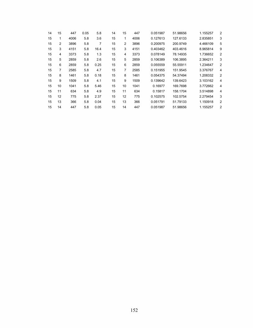
152

14 15 447 0.05 5.8 14 15 447 0.051987 51.98656 1.155257 2 15 1 4006 5.8 3.6 15 1 4006 0.127613 127.6133 2.835851 3 15 2 3896 5.8 7 15 2 3896 0.200975 200.9749 4.466109 5 15 3 4151 5.8 16.4 15 3 4151 0.403462 403.4616 8.965814 9 15 4 3373 5.8 1.3 15 4 3373 0.078149 78.14935 1.736652 2 15 5 2859 5.8 2.6 15 5 2859 0.106389 106.3895 2.364211 3 15 6 2859 5.8 0.25 15 6 2859 0.055559 55.55911 1.234647 2 15 7 2585 5.8 4.7 15 7 2585 0.151955 151.9545 3.376767 4 15 8 1461 5.8 0.18 15 8 1461 0.054375 54.37494 1.208332 2 15 9 1509 5.8 4.1 15 9 1509 0.139642 139.6423 3.103162 4 15 10 1041 5.8 5.46 15 10 1041 0.16977 169.7698 3.772662 4 15 11 634 5.8 4.9 15 11 634 0.15817 158.1704 3.514898 4 15 12 775 5.8 2.37 15 12 775 0.102575 102.5754 2.279454 3 15 13 366 5.8 0.04 15 13 366 0.051791 51.79133 1.150918 2 15 14 447 5.8 0.05 15 14 447 0.051987 51.98656 1.155257 2

153

Appendix C MPL SOGP Implementations North American network model – maximum growth 10x TITLE SOGP {11-Jun-05} INDEX n := 1..27; {nodes in network} i := n; j := n; r := 1..702; {index of demand pairs (traffic), each will have origination O[r] and destination T[r] as well as a demand value d} k := 0..6; {index of different switch sizes} DATA

CS[k]:= (0,1000,2000,4000, 10000, 20000,40000); {cost of switch chassis for each level of k}

cp[j] := DATAFILE("ConnectionCOSTcp.csv") ; {fixed cost of adding one

more connection to a switch j}

O[r] := SPARSEFILE("NAfulltraffic.csv", 2); { origin for rth demand}

T[r] := SPARSEFILE("NAfulltraffic.csv",3); { destination (termination) for rth demand}

D[r] := SPARSEFILE("NAfulltraffic.csv", 8); { Demand value or amount of traffic to be exchanged between origin, O, and destination, T, indexed by r}

cl[i,j] := SPARSEFILE("LINKCOST.csv"); { cost function for adding one unit of demand to each link in the model}

M := 10000000; {constant, larger than any switch capacity} VARIABLES

w[r,i,j] WHERE (cl); { working flow for each rth demand pair } lw[i,j] WHERE (cl); { total working flow one each i,j link } P[j]; { the number of connections needed in switch at node j to accommodate the traffic flow that will enter or leave this switch; switch capacity} S[j]; {cost of switch chassis at node j at level k through node j } BINARY VARIABLE

154

z[j,k]; {binary variable to match fixed cost of switch to correct size,k, if j is in model} MODEL

MIN TotalCost = SUM(j: (S[j])) + SUM(j: (cp[j] * P[j])) + SUM(i,j: (cl[i,j] * lw[i,j] )); SUBJECT TO { balance constraints - for each demand pair the total source flow equals the demand, the total sink flow equals the demand, and that no net sourcing or sinking of flow for the given O-D pair occurs at any other node (ie transshipment) }

Supply[r,i] where i=O[r]: SUM(j: w[r, i, j]) - SUM(j: w[r, i:=j, j:=i]) = D[r];

Demand[r,i] where i=T[r]: SUM(j: w[r, i, j]) - SUM(j: w[r, i:=j, j:=i]) = - D[r];

Balance[r,i] where i<>O[r] and i<>T[r]: SUM(j: w[r, i, j]) = SUM(j: w[r, i:=j, j:=i]) ;

{ link capacity constraint - defines total working capacity needed to deliver all traffic flow}

Capacity[i,j]: lw[i,j] = SUM(r: w[r,i,j]) ;

{total number of connections needed for switch at node j,port capacity}

PortCap[j]: P[j] >= SUM(i: lw[i,j]) + SUM(i: lw[i:=j,j:=i] );

{requires that if switch is not installed at j then there will be no connection cost}

Swconst[j]: P[j] <= M * (z[j,1] + z[j,2] + z[j,3] + z[j,4] + z[j,5] +z[j,6]);

{calculates the size of the switch chassis, at node j}

swstep[j]: P[j] <= 0*z[j,0] + 1000*z[j,1] + 2000*z[j,2] + 4000*z[j,3]+ 12000*z[j,4] + 24000*z[j,5] + 50000*z[j,6];

{calculates the cost of the switch, at node j}

155

swcost[j]: S[j] = (z[j,0]*CS[0] + z[j,1]*CS[1] + z[j,2]*CS[2] + z[j,3]*CS[3] + z[j,4]*CS[4] + z[j,5]*CS[5] +z[j,6]*CS[6]);

{constrains the size of switch chassis to no more than one size per node, if any at all}

swlimit[j]: SUM(k: z[j,k]) <= 1;

END

156

Appendix D – Skewness calculations

“Skewness is a measure of symmetry, or more precisely, the lack of symmetry. A

distribution, or data set, is symmetric if it looks the same to the left and right of the center

point.

Definition of Skewness For univariate data Y1, Y2, ..., YN, the formula for skewness is:

where is the mean, is the standard deviation, and N is the number of data points. The

skewness for a normal distribution is zero, and any symmetric data should have a

skewness near zero. Negative values for the skewness indicate data that are skewed left

and positive values for the skewness indicate data that are skewed right. By skewed left,

we mean that the left tail is heavier than the right tail. Similarly, skewed right means that

the right tail is heavier than the left tail. Some measurements have a lower bound and are

skewed right. For example, in reliability studies, failure times cannot be negative.”

http://www.itl.nist.gov/div898/handbook/eda/section3/eda35b.htm

Another variation on the formula for skewness that is used by Microsoft Excel is

Skewness = [n/ (n-1)(n-2)] * Σ[(Yi – Y)/s]3 where n is the number of data points,

Y is the mean, and s is the standard deviation.

VITA

Susan Jean Chinburg

Candidate for the Degree of

Doctor of Philosophy

Thesis: NODAL DISTRIBUTION STRATEGIES FOR DESIGNING AN OVERLAY NETWORK FOR LONG-TERM GROWTH Major Field: Business Administration Biographical:

Personal Data: Married Education: Bachelor of Science Teaching, General Science/Mathematics,Mankato State University, Mankato, MN, 1972, (junior high school earth science teaching and mathematics) Masters of Science, Geology, San Jose State University, San Jose, CA, 1985, Thesis: Sediment Dynamics of Monterey Submarine CanyonDoctorate of Philosophy, Business Administration, Oklahoma State University, Stillwater, OK, Completed the requirements for the PhD from Oklahoma State University in Dec 2006/graduation in Dec 2006 Experience: Visiting Professor and Instructor, College of Business and Applied Technology, Rogers State University, Claremore, OK Doctoral Teaching and Research Associate, Dept of Management Science and Information Sciences, Oklahoma State University, Stillwater, OK Engineer, Research and Development, Network Architecture, Williams Communications Group, Tulsa, OK Computer Lab Coordinator, Oklahoma State Univ., Stillwater, OK Systems Analyst and Research and Exploration Geologist, Conoco Inc, Research Scientist, Coastal Studies Institute, Louisiana State University, Baton Rouge, LA Professional Memberships: Sigma Beta Delta, business honor society, member Association for Information Systems, member and reviewer INFORMS, member IEEE, member

Name: Susan Jean Chinburg Date of Degree: December 2006 Institution: Oklahoma State University Location: Stillwater, Oklahoma Title of Study: NODAL DISTRIBUTION STRATEGIES FOR DESIGNING AN

OVERLAY NETWORK FOR LONG-TERM GROWTH Pages in Study: 156 Candidate for the Degree of Doctor of Philosophy Major Field: Business Administration Scope and Method of Study: This research looked at nodal distribution design issues associated with building an overlay network on top of an existing legacy network with overlay network switches and links not necessarily matching the switch and link locations of the underlying network. A mathematical model with two basic components, switch costs and link costs, was developed for defining the total cost of a network overlay. The nature of the underlying legacy topology determines the dominant factor, link or switch costs to the total cost function as well as the unit cost for switches and links.

Findings and Conclusions:

The three design heuristics presented first, locate overlay switches at nodes in the center of the legacy network as opposed to the periphery; second, locate overlay switches at legacy nodes with high connectivity; and third, locate overlay switches at legacy nodes with high traffic flow demands, can be used to help point to the direction of keeping costs under control when design changes are required. Applying the concept of efficient frontiers to the world of network design and building a suite of best designs gives the network designer greater insight into how to design the best network in the face of changing real-world constraints. For the cost model and the case studies evaluated using the design strategies in this study, distributed approaches generally tend to be a good choice when the link costs dominate the total cost function because total path distances and therefore link costs need to be minimized in preference over switch costs. A distributed overlay tends to have lower link costs because there is usually a greater probability that total path distances can be minimized because of greater connectivity. More connections set up the potential for more traffic flow path choices allowing each traffic flow to be sent along shorter paths. In legacy network topology designs that have many nodes with high connectivity, the overlay link costs can be relatively similar between designs and the switch costs can have a large impact upon total cost.

ADVISER’S APPROVAL: Dr. George Scheets