noise and vibration control for - cloud object storage ...€¦ · guide b provides guidance on the...
TRANSCRIPT


Noise and vibration control for building services systems
CIBSE Guide B4: 2016
The Chartered Institution of Building Services Engineers
222 Balham High Road, London, SW12 9BS
This publication is supplied by CIB
SE
for the sole use of the person making the dow
nload. The content remains the copyright of C
IBS
E.

Note from the publisherThis publication is primarily intended to provide guidance to those responsible for the design, installation, commissioning, operation and maintenance of building services. It is not intended to be exhaustive or definitive and it will be necessary for users of the guidance given to exercise their own professional judgement when deciding whether to abide by or depart from it.
Any commercial products depicted or describer within this publication are included for the purposes of illustration only and their inclusion does not constitute endorsement or recommendation by the Institution.
The rights of publication or translation are reserved.
No part of this publication may be reproduced, stored in a retrieval system or transmitted in any form or by any means without the prior permission of the Institution.
© June 2016 The Chartered Institution of Building Services Engineers London
Registered charity number 278104
ISBN 978-1-906846-79-4 (book)
ISBN 978-1-906846-80-0 (PDF)
This document is based on the best knowledge available at the time of publication. However no responsibility of any kind for any injury, death, loss, damage or delay however caused resulting from the use of these recommendations can be accepted by the Chartered Institution of Building Services Engineers, the authors or others involved in its publication. In adopting these recommendations for use each adopter by doing so agrees to accept full responsibility for any personal injury, death, loss, damage or delay arising out of or in connection with their use by or on behalf of such adopter irrespective of the cause or reason therefore and agrees to defend, indemnify and hold harmless the Chartered Institution of Building Services Engineers, the authors and others involved in their publication from any and all liability arising out of or in connection with such use as aforesaid and irrespective of any negligence on the part of those indemnified.
Design, layout and typesetting by CIBSE Publications
Printed in Great Britain by Page Bros. (Norwich) Ltd., Norwich, Norfolk NR6 6SA
This publication is supplied by CIB
SE
for the sole use of the person making the dow
nload. The content remains the copyright of C
IBS
E.

ForewordGuide B provides guidance on the practical design of heating, ventilation and air conditioning systems. It represents a consensus on what constitutes relevant good practice guidance. This has developed over more than 70 years, with the Steering Groups for each edition of the Guide expanding and pruning the content to reflect the evolution of technology and priorities.
Since the last edition of Guide B in 2005, the European Energy Performance of Buildings Directive has been introduced. This requires national building energy regulations to be based on calculations that integrate the impact of the building envelope and the building services systems, formalising what was already recognised as good design practice. In addition, the use of voluntary energy efficiency and sustainability indicators has increased.
These changes have influenced the content of Guide B, but the emphasis remains on system design. The guidance in Guide B is not in itself sufficient to cover every aspect of the effective design of hvac systems. Energy (and carbon emission) calculations will also be needed, and a range of other environmental criteria may specified by the client. These may, for example, include whole-life costing or assessments of embodied energy or carbon. The balance between building fabric measures and the energy efficiency of hvac systems is important, as is the balance between energy use for lighting and for heating, ventilation and cooling. More detailed information on energy efficiency and sustainability can be found in Guides F and L respectively. The Guide does not attempt to provide step by step design procedures: these can be found in appropriate textbooks.
Structure of CIBSE Guide BGuide B deals with systems to provide heating, ventilation and air conditioning services, and is divided into several chapters which are published separately. It will usually be necessary to refer to several — perhaps all — chapters since decisions based on one service will commonly affect the provision of others.
— Chapter B0: Applications focuses on how different types of building and different activities within buildings influence the choice of system. This chapter is not available in printed form, but can be downloaded from the CIBSE website. For many activities and types of building, more detailed design information is available in specialist guidance.
Chapters B1 to B4 address issues relating to specific services. There are usually several possible design solutions to any situation, and the Guide does not attempt to be prescriptive but rather to highlight the strengths and weaknesses of different options.
— B1: Heating, including hot water systems and an appendix on hydronic system design, which is also applicable to chilled water systems
— B2: Ventilation and ductwork
— B3: Air conditioning and refrigeration
— B4: Noise and vibration control for building services systems (applicable to all systems)
When all chapters have been published, an index to the complete Guide B will be made available.
The focus is on application in the UK: though many aspects of the guidance apply more generally, this should not be taken for granted. The level of detail provided varies: where detailed guidance from CIBSE or other sources is readily available, Guide B is relatively brief and refers to these sources. Examples of this are the treatment in the Guide of low carbon systems such as heat pumps, solar thermal water heating and combined heat and power. On-site energy generation such as wind power and photovoltaics are not covered.
Regulatory requirements are not described in detail in the Guide — the information varies between jurisdictions and is liable to change more rapidly than the Guide can be updated. Instead, the existence of regulations is sign-posted and their general scope explained. Sometime example tables are shown, but readers should note that these are simply examples of the type of requirement that is imposed and may not be current.
While there is some discussion of relative costs, no attempt is made to provide detailed cost figures as these are too project-specific and variable with time and location.
Roger Hitchin Chair, CIBSE Guide B Steering Committee
This publication is supplied by CIB
SE
for the sole use of the person making the dow
nload. The content remains the copyright of C
IBS
E.

Guide B4 Steering CommitteeBob Peters (Chair) Applied Acoustic Design Ltd and visiting research fellow at London South Bank UniversityAlan Fry SalexRichard Galbraith Sandy Brown Associates LLPPeter Henson Bickerdike Allen PartnersAlex Krasnic Vanguardia ConsultingJohn Lloyd Scotch Partners LLPJohn Shelton AcSoftPeter Tucker Impulse Acoustics Ltd
The Steering Committee acknowledges the particular contribution of their late colleague, Peter Tucker, who passed away while this document was being prepared for publication.
AcknowledgementsPermission to reproduce extracts from British Standards is granted by BSI Standards Ltd. British Standards can be obtained in pdf or hard copy formats from BSI online shop: www.bsigroup.com/Shop or by contacting BSI Customer Services for hardcopies only: tel: +44 (0)20 8996 9001, e-mail: [email protected].
Public information is reproduced under Open Government Licence v2.0.
RefereesRichard Cowell ArupMark Saunders Allaway AcousticsKeith Shenstone Imtech
EditorEd Palmer
Editorial ManagerKen Butcher
CIBSE Technical DirectorHywel Davies
CIBSE Head of KnowledgeNicholas Peake
This publication is supplied by CIB
SE
for the sole use of the person making the dow
nload. The content remains the copyright of C
IBS
E.

Contents
4.1 Introduction 4-1
4.1.1 Preamble 4-14.1.2 Mechanisms of noise generation, noise sources and transmission paths 4-14.1.3 Overview and structure of the Guide 4-2
4.2 Summary of noise and vibration problems from hvac 4-3
4.2.1 Typical sources of hvac noise and their characteristics 4-34.2.2 Transmission paths 4-34.2.3 Control of the transmission paths 4-5
4.3 Noise sources in building services 4-5
4.3.1 Introduction 4-54.3.2 Fans 4-64.3.3 High velocity/high pressure terminal units 4-84.3.4 Grilles and diffusers 4-94.3.5 Fan coil units 4-114.3.6 Induction units 4-124.3.7 Air conditioning units 4-134.3.8 Fan-assisted terminal units 4-144.3.9 Rooftop units/air handling units 4-174.3.10 Acoustic louvres 4-204.3.11 Chillers and compressors 4-214.3.12 Pumps 4-214.3.13 Boilers 4-214.3.14 Heat rejection and cooling towers 4-224.3.15 Chilled ceilings 4-224.3.16 Lifts 4-244.3.17 Escalators 4-254.3.18 Electric motors 4-264.3.19 Noise from water flow systems 4-26
4.4 Noise control in plant rooms 4-27
4.4.1 Risk of noise induced hearing loss 4-274.4.2 Breakout noise from plant rooms 4-284.4.3 Break-in noise in plant rooms 4-294.4.4 Estimation of noise levels in plant rooms 4-29
4.5 Airflow noise – regeneration of noise in ducts 4-29
4.5.1 Flow rate guidance 4-294.5.2 Prediction techniques 4-294.5.3 Damper noise 4-314.5.4 Turbulence-induced noise in and from ductwork 4-31
4.6 Control of noise transmission in ducts 4-36
4.6.1 Duct components 4-364.6.2 Unlined straight ducts 4-364.6.3 Lined straight ducts 4-364.6.4 Duct bends 4-364.6.5 Duct take-offs 4-394.6.6 End reflection loss 4-394.6.7 Passive attenuators and plenums 4-404.6.8 Active attenuators 4-45
This publication is supplied by CIB
SE
for the sole use of the person making the dow
nload. The content remains the copyright of C
IBS
E.
4.6.9 Use of fibrous sound absorbing materials in ducts 4-464.6.10 Duct breakout noise 4-464.6.11 Duct break-in noise 4-484.6.12 Attenuator noise break-in 4-51
4.7 Room sound levels 4-52
4.7.1 Behaviour of sound in rooms 4-524.7.2 Determination of sound level at a receiver point 4-524.7.3 Source directivity 4-554.7.4 Sound transmission between rooms 4-564.7.5 Privacy and cross talk 4-57
4.8 Transmission of noise to and from the outside 4-59
4.8.1 Transmission of noise to the outside and to other rooms 4-594.8.2 Transmission of external noise to the inside 4-594.8.3 Naturally ventilated buildings 4-59
4.9 Criteria for noise from building services systems 4-60
4.9.1 Objective 4-604.9.2 Choosing noise criteria parameters 4-604.9.3 Design criteria 4-614.9.4 Using dBA, dBC, NR and Nc levels 4-61
4.10 Noise prediction of sound pressure levels from building services 4-63
4.10.1 Room effect 4-634.10.2 System noise 4-654.10.3 Breakout/break-in noise 4-664.10.4 Noise propagation to outdoors 4-67
4.11 Vibration problems and control 4-69
4.11.1 Introduction 4-694.11.2 Fundamentals of vibration and vibration control 4-704.11.3 Rating equipment for vibration emission 4-724.11.4 Vibration isolation criteria 4-734.11.5 Common types of vibration isolator 4-764.11.6 Practical examples of vibration isolation 4-80
4.12 Summary 4-88
4.12.1 Noise in HVAC systems 4-884.12.2 Vibration in HVAC systems 4-88
Appendix 4.A1: Explanation of some basic acoustic concepts 4-90Appendix 4.A2: Regeneration of noise by duct components and terminations 4-96Appendix 4.A3: Interpreting manufacturers’ noise data 4-99Appendix 4.A4: Noise instrumentation 4-100Appendix 4.A5: Vibration instrumentation 4-104Appendix 4.A6: Uncertainty in measurement and prediction of sound levels and sound power levels 4-107Appendix 4.A7: Application of noise prediction software and integrated building design processes 4-108Appendix 4.A8: Glossary 4-109
Index 4-133
This publication is supplied by CIB
SE
for the sole use of the person making the dow
nload. The content remains the copyright of C
IBS
E.

Introduction 4-1
4.1 Introduction
4.1.1 Preamble
This document, which forms chapter 4 of CIBSE Guide B, provides guidance to building services engineers and others involved in the design of building services on the generation, prediction, assessment and control of noise and vibration from building services, so that designers may produce systems which meet acceptable noise limits. Noise reduction procedures are always much more effective and economic when introduced at the design stage than when applied retrospectively. Therefore it is important that the issue of noise is taken into account at an early stage of the design process, involving advice from an acoustics expert in particularly noise sensitive situations.
Other chapters of CIBSE Guide B relate to heating (B1 (2016a)), ventilation (B2 (2016b)) and refrigeration and air conditioning (B3 (2016c)), so although this chapter is self-contained it is also intended to provide support to users of these chapters in matters relating to noise and vibration.
The aim of this chapter is to provide guidance to enable building services systems to be designed to achieve acceptable levels of noise in addition to meeting requirements relating to aerodynamics, energy usage and economics.
This chapter cannot and is not intended to be a comprehensive textbook on the subject and an extensive reference list has been provided for those needing more detailed information.
More information on noise is provided in CIBSE Guide A, sections 1.9 and 1.10, which discuss the subjective effects of noise and vibration and its assessment. Table 1.5 in Guide A suggests limits for noise from building services in various spaces. Useful information is also contained in CIBSE TM40: Health issues in building services (2006a), TM42: Fan application guide (2006b) and TM43: Fan coil units (2008).
This revised version replaces chapter 5 of the 2005 edition of Guide B. Although the structure of the previous version has been largely been retained, many of the individual sections have been revised and updated and additional material has been provided relating to natural ventilation.
A glossary of terms and appendices on uncertainties in measurement and prediction of noise levels, and on use of noise prediction software and integrated building design processes have also been added. The section on noise criteria has been rewritten so that it complements the material in chapter 1 of CIBSE Guide A.
4.1.2 Mechanisms of noise generation, noise sources and transmission paths
Noise from building services can cause annoyance and disturbance to the occupants inside the building and to those outside. In order to minimise such problems it is first necessary to set limits for building services noise and then to design the services systems to achieve these limits. In addition, it is necessary to achieve all other requirements relating to aerodynamics, airflow, air quality, cost and minimum energy usage.
Achieving the target noise limit requires knowledge and understanding of how building services noise is generated and transmitted to those affected by it, so that noise levels may be minimized by good design. It also requires that noise levels can be predicted so that system designs can be modified as necessary to achieve noise targets.
In a mechanically ventilated building, an air handling unit in a plant room delivers air to ventilated spaces in the building (e.g. offices, hotel bedrooms etc.) via a duct system, which is also an efficient transmitter of noise from the fan into each of these spaces.
The duct system consists of straight lengths of duct, bends, branches, terminal units, grilles and diffusers, dampers, and silencers to reduce noise. Each component of the system (i.e. each straight duct run, bend, etc.) provides some attenuation of the noise travelling towards the ventilated space but in addition may also provide some additional flow generated noise. There may also be some interaction between the components of the system so that their performance in combination may be different to that in isolation.
Noise generated by airflow increases greatly when the flow becomes turbulent, which can happen when sudden changes in airflow direction occur (e.g. at changes of cross section, at bends and branches and through terminal units). Therefore a general principle of low noise design is that airflow should be kept as smooth as possible and that air velocities should, within certain limits, be kept as low as possible.
The noise level prediction process involves tracking the flow of sound energy from the fan in the plant room through each component of the system, taking account of the sound attenuation and additional flow generated noise provided at each stage. In the final stage of the process the total sound power entering the ventilated room via the grille or diffuser is converted into a sound pressure level at the position occupied by the occupant. This process is indicated schematically in Figure 4.1 and a more representational
4 Noise and vibration control for building services systems
This publication is supplied by CIB
SE
for the sole use of the person making the dow
nload. The content remains the copyright of C
IBS
E.

4-2 Noise and vibration control for building services systems
diagram, illustrating the flow of sound energy through a heating, ventilation and air conditioning (hvac) system in a building is shown in Figure 4.3 below and discussed in more detail in section 4.2.
An important purpose of the prediction process is to specify the additional noise attenuation required of the silencers in the system (i.e. in addition to that provided by the other duct system components) in order that the predicted sound pressure level in the room shall meet the required noise target. The main primary silencers are located close to the fan, in the plant room, and designed to attenuate low and medium frequency sound produced by the fan. Smaller secondary silencers, if needed, are located close to the ventilated space to attenuate any disturbing residual fan noise together with accumulated flow generated noise, and also to reduce problems of ‘crosstalk’ between adjacent ventilated rooms.
In addition to that transmitted via the duct system there are other paths for hvac noise to reach occupants, such as via noise breakout through the duct walls, and airborne and structure-borne transmission from fan generated noise and vibration.
Although noise from hvac systems is a major source of building services noise there are many other sources including boilers, pumps, lifts, escalators, heat rejection plant, hydraulic systems. These are discussed in section 4.3. Some of these sources may be located inside the ventilated space (e.g. fan coil units, fans in personal computers) and in other cases noise from sources outside the space may be transmitted to the occupants of the space by airborne or structure borne paths.
All these sources and transmission paths must be considered by the designer and incorporated into the noise level prediction process.
The noise level prediction process requires information about the noise emission from the fan, and other noise sources, and about the noise attenuation (insertion loss) and flow generated noise emission provided by each component of the duct system. The accuracy of the prediction process will depend on the reliability and accuracy of this input data. Manufacturers’ data, which should be based on British or International Standard test procedures, should always be used, and if not available an alternative product should be used, for which such data is available. In the early stages of design, before manufacturers’ data is available, the designer may need to use generic data in order to predict noise levels and to refine the design to meet noise criteria. Some typical values of such generic data are described in sections 4.3 and 4.6. Once the design
is finalized sensitivity predictions should be carried out using manufacturers’ data.
Fan manufacturers’ noise emission data are measured under idealised test conditions to deliver minimum possible levels of noise, in particular with streamlined flow of air supply into the fan. These conditions may not be always reproduced in practical applications and as a result noise emission may be higher than indicated by the test data. In addition the test data may be expressed in a variety of different ways (e.g. either as a sound power level or as a sound pressure level at a specified distance, and either with or without A-weightings). The designer must carefully consider these issues.
Consideration must be given by the designer to the transmission of building services noise, in all its forms, to the outside environment, where it may adversely affect neighbours.
Noise may also be transmitted into the building from outside to combine with that produced by the building services. This may be one of the factors determining the selection of a maximum noise target set for the noise from the building services, so that in combination with noise from outside a satisfactory total level of noise is achieved within the building. Ingress of external noise will be particularly important in the case of naturally ventilated buildings.
There may be some situations where the levels of both building services noise and external noise ingress are so low that the conversations of occupants may be intelligible over considerable distances, giving rise to problems of speech privacy. In such cases it may be necessary to introduce additional ambient sound to mask speech from occupants so that adequate levels of speech privacy are restored. Commercial sound masking systems are available for this purpose.
The building services engineer should be aware of all these various noise related issues which can affect the comfort of those inside and outside the building and if not responsible for all of them (e.g. if only responsible for the hvac system) should inform and liaise with those (e.g. architects) who have this responsibility.
4.1.3 Overview and structure of the Guide
Section 4.2 summarizes some of the main problems that can arise from hvac systems. It gives an overview of the frequency characteristics of the main noise sources and then describes the various sound transmission paths to receivers, and how they may be controlled
Section 4.3 describes in detail the various noise sources arising from the provision of building services: fans, variable air volume (vav) systems, grilles and diffusers, roof top units, fan coils units, chillers, compressors and condensers, pumps, standby generators, boilers, cooling towers and lifts and escalators. This section contains a great deal of detailed information about noise emission data in the form of graphs and formulae and tables, enabling typical values of sound pressure levels and sound power levels to be estimated. This information will be of use to the
WP
Duct system
Sound power
Sound attenuation
Othersources
RoomAN
Otherpaths
A3A2A1
A
WS2WS2
W
Figure 4.1 The flow of sound energy in an hvac system
This publication is supplied by CIB
SE
for the sole use of the person making the dow
nload. The content remains the copyright of C
IBS
E.
Summary of noise and vibration problems from hvac 4-3
designer in the early stages of design, before manufacturers’ test-based data is used in the final stage of design.
Section 4.4 considers noise control in plant rooms, first describing the health and safety requirements for employees in plant rooms, the methods for estimating and reducing plant room noise, breakout of plant room noise to adjacent areas and to the outside, and the effective positioning of plant room silencers to minimise such transmission.
Section 4.5 describes the mechanisms of airflow generated noise, also called regenerated noise, in ducts and associated fittings, and how it may be predicted. It also describes good practice for avoiding turbulent airflow and therefore minimizing flow generated noise from branches, bends, grille and diffusers and self-noise from silencers.
Section 4.6 expands on the summary given in section 4.2 to describe in detail the techniques for control of noise transmission in ducts. The methods for determining the attenuation for the various components of the duct system are described: straight ducts, bends, branches, distribution boxes (plenums) and terminal units (grilles and diffusers). The use of passive and active silencers are described, together with guidance on the use of fibrous materials to absorb sound in ducts. Having considered how to minimise sound transmission via the duct system this part of the Guide concludes with advice about predicting and minimizing noise breakout from ducts. This section contains a great deal of detailed guidance and information about noise attenuation data in the form of graphs, tables and formulae which will be of use to the designer. As with the information in section 4.3 this information will be useful in the early stages of design but manufacturers’ specific product data should always be used, when available.
Section 4.7 is another major section of the Guide, on predicting and controlling sound levels in rooms with some of the details being given in Appendix 4.A2. The effects of speech interference and speech privacy are also discussed.
Section 4.8 of the Guide deals with transmission of noise to and from the outside including naturally ventilated buildings.
Section 4.9, which has been completely rewritten, discusses the use of noise criteria for the assessment of noise in building services systems. The assessment of building services noise is also discussed in more detail in CIBSE Guide A sections 1.9 and 1.10, and Table 1.5 gives guidance on recommended maximum noise levels for various types of indoor spaces.
Section 4.10 outlines the steps in the method for the prediction of noise levels with the details of the calculations given in the appendices.
Section 4.11, a major part of the Guide, describes the fundamentals of vibration and of vibration control in building services plant. The practical aspects of vibration isolation are also described.
Section 4.12 concludes the main part of the Guide with a summary of the guidance on noise and vibration.
There are a number of appendices, a glossary of terms and a list of reference material.
4.2 Summary of noise and vibration problems from hvac
4.2.1 Typical sources of hvac noise and their characteristics
Noise is produced by vibrating surfaces and by moving air streams. Sometimes the two interact, as in the case of fan blades. The primary source of the noise normally lies in the rotation of a machine, such as a motor, pump or fan. However, energy imparted to air or water can be converted into noise through interaction of fluid flow with solid objects, e.g. louvres in a duct termination. A very broad generalisation is that the ‘noise conversion efficiency’ of a machine is around 10–7 of its input power, but there are wide variations above and below this figure, while aerodynamic noise increases rapidly with air velocity. A fan, which contains both drive motor and fan wheel, is more likely to convert around 10–6 of its input power to noise. Sound powers are low in terms of wattage but, because of the sensitivity of the ear, only milliwatts of acoustic power are required to produce a loud noise (see Appendix 4.A1).
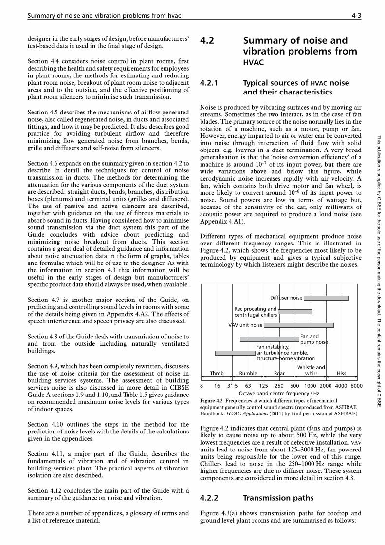
Different types of mechanical equipment produce noise over different frequency ranges. This is illustrated in Figure 4.2, which shows the frequencies most likely to be produced by equipment and gives a typical subjective terminology by which listeners might describe the noises.
80004000200010005002501256331·5168Octave band centre frequency / Hz
Diffuser noise
Reciprocating andcentrifugal chillers
VAV unit noise
Fan andpump noise
Throb
Fan instability, air turbulence rumble,structure-borne vibration
Rumble RoarWhistle and
whirr Hiss
Figure 4.2 Frequencies at which different types of mechanical equipment generally control sound spectra (reproduced from ASHRAE Handbook: HVAC Applications (2011) by kind permission of ASHRAE)
Figure 4.2 indicates that central plant (fans and pumps) is likely to cause noise up to about 500 Hz, while the very lowest frequencies are a result of defective installation. vav units lead to noise from about 125–3000 Hz, fan powered units being responsible for the lower end of this range. Chillers lead to noise in the 250–1000 Hz range while higher frequencies are due to diffuser noise. These system components are considered in more detail in section 4.3.
4.2.2 Transmission paths
Figure 4.3(a) shows transmission paths for rooftop and ground level plant rooms and are summarised as follows:
This publication is supplied by CIB
SE
for the sole use of the person making the dow
nload. The content remains the copyright of C
IBS
E.

4-4 Noise and vibration control for building services systems
Figure 4.3 Noise from rooftop and ground level plant; (above) transmission paths, (below) possible means of attenuation
5 5
33
1
4
2 2
2 2
2444
5 5
5
3
3
2 2
Attenuator
CRITICAL AREA
Noiseblocking
fromshafts
Smoothtake-offs
Noise stop pads Resilient floatingfloor supports
Inertia block
Springisolators
Floatingfloor
Plant room noise absoption
Inertiablock
Springisolators
Terminal unit in ceiling void
Crosstalk attenuator
Floating floor
Resilient clamps
High sound reduction performance wall
Acoustic louvre
Flexible connector Resilient hanger
Acoustic louvre
This publication is supplied by CIB
SE
for the sole use of the person making the dow
nload. The content remains the copyright of C
IBS
E.
Noise sources in building services 4-5
— noise radiates to atmosphere from the air inlet or outlet (path 1)
— vibration from the fan transmits to the structure (path 5)
— noise from the plant breaks out of the plant room (path 3)
— noise may break out of the supply duct to adjacent spaces (path 2)
— incorrect duct or pipe anchoring may put vibra tion into the structure (path 5)
— duct borne noise is emitted from the room units (path 4)
— vibration from ground level plant gets into the structure (path 5)
— noise from plant transmits through walls or windows to adjacent spaces (path 2).
In controlling the noise of the hvac plant, all transmission paths must be assessed for their contribution to the final noise in occupied spaces and the paths controlled accordingly. Figure 4.3(b) illustrates some possible solutions.
4.2.3 Control of the transmission paths
This section considers some general principles of good practice in noise and vibration control in hvac. More details are given in sections 4.4, 4.5, 4.6 and 4.11. The preferred way to control noise is to prevent it occurring in the first place, but some noise generation is unavoidable from realistic airflow velocities. In hvac systems, controlling noise means:
— choosing the operating condition of the fan so that it is at a high efficiency point on its fan performance curve; this minimises fan noise
— ensuring good flow conditions for the air stream; benefits include components behaving closer to descriptions in the manufac turers’ data, and reduced pressure losses, which conserves energy and lowers operating costs
— isolating vibrating components, including all machinery, ducts and pipework from the structure
— choosing an in-duct silencer or other means to control airborne noise in ducts (refer to BS EN ISO 14163 (BSI, 1998)); a full silencer may not be required, as lining bends with acoustic absorbent may be adequate, but this depends on the results of noise predictions (see section 4.10).
Noise control relies on attention to detail, both in the design and the implementation. It depends on choosing the correct components and ensuring that they are installed correctly.
There are many instances of problems which have resulted from inadequacies in design and installation, including:
— undersized fans, which could not accept the pressure loss of retrofit silencers
— oversized fans, which were working on an undesirable part of their characteristic
— vibration isolators which were bypassed by solid connections
— unsealed gaps around penetrations which allow airborne noise transmission.
4.3 Noise sources in building services
4.3.1 Introduction
There are a large number of potential noise sources in a building services installation, including fans, duct components, grilles and diffusers, plant (such as chillers, boilers, compressors, cooling towers, condensers, pumps, standby generators), lifts and escalators. A tendency for design practice to move away from central plant to local systems, often positioned in the ceiling void, has brought noise sources closer to occupants and increased the problems of noise reaching occupied rooms. Noise from a plant room, especially large central plant, may break out to the exterior and be a source of annoyance to neighbours. Nuisance to neighbours comes under the responsibility of the local environmental health department, which may require the noise to be abated. Local authorities often apply conditions to planning consents in order to protect neighbours from nuisance caused by building services plant. Such conditions must be complied with.
Prediction formulae have been established for some items of plant by measurements on a sample of the plant. Much of this work was carried out many years ago, when information was not available from manufacturers. Since that time designs have changed. There have been efforts by the larger manufacturers of plant to reduce plant noise, while most manufacturers have also become aware of the need to provide data on the noise of their plant. The main source of information on noise is now the manufacturer. Inability, or reluctance, to provide such information might influence the choice of manufacturer.
The measurement conditions for plant noise must be specified along with the relation of the measurement procedure to standardised methods. It should be remembered that the installation conditions may not be the same as the measurement conditions and that there are uncertainties in measurement, especially at low frequencies.
In the very early stages of a project, plant may not have been fully specified and, only under such circumstances, generic noise data may be used for outline consideration of noise control measures, e.g. spatial requirements for attenuators. Generic prediction information is given in Appendix 4.A2, which must be regarded as for temporary use only, until equipment-specific information is available. The uncertainties of generic information are at least ±5 dB, and often greater.
There are many items of building services plant which generate noise, including recent technologies such as ground source heat pumps and combined heat and power installations. This chapter confines itself to considering the following items of equipment:
This publication is supplied by CIB
SE
for the sole use of the person making the dow
nload. The content remains the copyright of C
IBS
E.
4-6 Noise and vibration control for building services systems
— fans
— high velocity/high pressure terminal units
— grilles and diffusers
— fan coil units
— induction units
— roof top units air cooled chillers and condensers
— pumps
— standby generators
— boilers
— heat rejection equipment and cooling towers
— chilled ceilings
— lifts
— escalators
— electric motors.
4.3.2 Fans
Control of fan noise depends on:
— choosing an efficient operating point for the fan
— design of good flow conditions
— ensuring that the fan is vibration isolated from the structure
— ensuring that the fan is flexibly connected to the duct.
Where fan noise will be a problem, an in-duct attenuator should be used. These are described in detail in section 4.6.
4.3.2.1 Fan noise sound power level, LW
If a fan has been selected from a manufacturer, then the safe working limit (swl) data from that manufacturer, for the given installation situation, should be adopted. This will preferably be based on tested data.
However, in most situations demanding an early estimate of a systems sound predictions, only the duty (pressure and flow rate) and fan type (centrifugal with suggested blade type, axial, mixed flow or propeller) will have been established.
The following method for making such an estimate, is more detailed and, as an estimate, more accurate for guidance than a popular method attributed to Beranek (1992).
This scheme gives the guidance for the in duct fan sound power level, LW, as follows:
LW = LWs +10 lg Q + 20 lg P + 40 + bfi + C
(4.1)
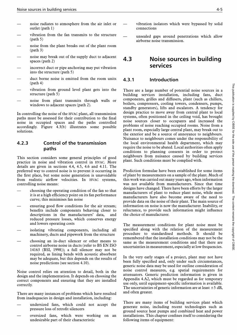
Where LWs is the sound power level correction (and includes the basic spectrum shape for each fan type), Q is the fan volume flow rate (m3/s), P is the fan static pressure (N/m2), bfi is the blade frequency increment (dB) and C is the fan efficiency correction factor (dB).
4.3.2.2 Method for calculating fan noise sound power level, LW
(1) From the fan volume flow rate and the pressure, determine the reference sound power level from Figure 4.4, which covers the terms (10 lg Q + 20 lg P + 40).
(2) From Table 4.1 determine the spectrum correction term, LWs, for the particular type and size of fan proposed. Add these corrections to the reference sound power level of step 1 (noting the negative (–) signs in this table). This gives the basic sound power level. (For reference, octave band width values are supplied in Table 4.4.)
(3) Determine the bfi, from the far right hand column of Table 4.1, for the octave in which the blade passage frequency (Bf), occurs.
Bf (Hz), can be calculated from:
fan speed (r/min) × number of blades Bf = ————————————––——— 60
or, if this information is not available, Table 4.2 provides the usual values for Bf.
(4) Apply the correction factor C, for off peak fan operation, from Table 4.3.
When the final fan selection has been made, a comparison of the predicted and submitted manufacturers’ data will allow the differences to be incorporated.
4.3.2.3 Centrifugal fan casing breakout noise
To estimate the sound power output through the casing of a centrifugal fan, the values given in Table 4.5 below (in dB) should be subtracted from the total sound power level of the fan. Note that ‘total’ means inlet plus outlet sound power level and at its simplest should be considered as 3 dB
Figure 4.4 Graph for term 10 lg10 Q + 20 lg10 P + 40
130
120
110
100
90
80
70
60
50
Refe
renc
e so
und
pow
er le
vel /
db
re. 1
0–12
W
Volume flow / (m3/s)0 0·2 0·4 0·8 1·0 2·0 4·0 6·0 10.0 20·0 40·0
10 N·m215 N·m220 N·m230 N·m240 N·m260 N·m2100 N·m
2150 N·m2200 N·m2300 N·m2400 N·m2600 N·m21000 N·m
21500 N·m
22000 N·m
23000 N·m24000 N·m2
6000 N·m210 000 N·m
2
Fan pressure
This publication is supplied by CIB
SE
for the sole use of the person making the dow
nload. The content remains the copyright of C
IBS
E.

Noise sources in building services 4-7
Table 4.2 Octave band in which bfi occurs for various fan types
Fan type Octave band (/ Hz) in which bfi occurs for stated fan speed / (r/min)
<1750 >1750
Centrifugal 250 500
Aerofoil (backward curved, backward inclined, forward curved) 500 1000
Radial blade, pressure blower 125 250
Vaneaxial 125 250
Tubeaxial 63 125
Propeller 63 125
Table 4.3 Correction factor (C) for off peak operation
Static efficiency / % off peak Correction factor / dB
90–100 0
85–89 3
75–84 6
65–74 9
55–64 12
50–54 15
Table 4.1 Sound power spectrum corrections and blade frequency increments (bfi) for fans of various types
Fan type Wheel size / m
Sound power spectrum corrections, LWs / dB for stated octave centre band frequency / Hz
bfi / dB
63 125 250 500 1000 2000 4000
Centrifugal: aerofoil, backward curved, backward inclined
>0.9 –23 –23 –24 –26 –27 –32 –40 3<0.9 –17 –17 –19 –21 –22 –27 –35 3
Centrifugal: forward curved All –8 –12 –14 –22 –27 –30 –32 2
Centrifugal: radial blade >1 –10 –16 –13 –16 –18 –23 –25 8
Pressure blower 1 to 0.5 0 –7 –7 –10 –10 –15 –17 8<0.5 8 2 –3 –5 –11 –16 –19 8
Vaneaxial (flared supports) >1 –16 –19 –17 –16 –18 –21 –23 6<1 –18 –16 –12 –12 –12 –14 –17 6
Tubeaxial (tie rods supports) >1 –14 –16 –12 –14 –16 –18 –21 5<1 –15 –14 –8 –9 –11 –12 –18 5
Propeller (cooling tower) All –7 –4 –3 1 0 –3 –9 5
Table 4.4 Octave band width value
Octave band centre frequency
/ Hz
Band width / Hz
16 11.0 – 22
31.5 22.1 – 44
63 44.1 – 88
125 88.1 – 176
250 177 – 353
500 354 – 707
1000 707.1 – 1414
2000 1415 – 2828
4000 2829 – 5657
8000 5658 – 11313
16000 11314 – 22627
Table 4.5 Centrifugal fan casing breakout noise (reproduced courtesy of Buffalo Forge)
Casing thickness / mm
Breakout noise / dB for stated octave frequency band / Hz
63 125 250 500 1000 2000 4000 8000
2 16 16 16 16 16 16 16 162.6 18 18 18 18 18 18 18 18
3 19 19 19 19 19 19 19 194 20 20 20 20 20 20 20 20
6 22 22 22 22 22 22 22 229 25 25 25 25 25 25 25 25
12 27 27 27 27 27 27 27 2718 30 30 30 30 30 30 30 30
This publication is supplied by CIB
SE
for the sole use of the person making the dow
nload. The content remains the copyright of C
IBS
E.
4-8 Noise and vibration control for building services systems
more than the inlet or outlet sound power levels. Where manufacturers’ data are available they should of course be used.
4.3.3 High velocity/high pressure terminal units
These units or ‘boxes’, which cover a large volume flow rate range from 0.02–3.00 m3/s, are usually located in the ceiling void of the ventilated area and connected to a local ductwork distribution system in this void to the outlet or inlet diffusers. The larger units can sometimes be accommodated in risers or spaces adjacent to the conditioned area which can assist the noise control procedures. While these are usually implemented on both the supply and extract sides, the supply side can demand a higher degree of system attenuation.
High velocity terminal units originate from a concept to distribute larger quantities of conditioned air through a ductwork system. This type of operation was shown to be more feasible than other established low velocity systems, which operated at around 4 m/s in the main ductwork and dropping down to less than 0.5 m/s in the final outlet ducts to the grilles and diffusers.
The prime distribution ductwork speeds are increased to as much as 20 m/s and this necessarily requires higher system pressures up to 2000 Pa. Often cylindrical ductwork systems are adopted but rectangular ductwork is still employed and also the compromised ‘oval ductwork’ concept.
Hence, before the conditioned air can approach the grille/diffuser it requires to be slowed and the higher pressure reduced.
4.3.3.1 Variable air volume (VAV) and constant volume (CV) systems
For this purpose high velocity terminal units can contain a pressure reduction valve in conjunction with a noise attenuation element. This valve may be a ‘constant volume’ preset valve, which adjusts to accommodate any changing applied pressure changes to hold the volume flow rate constant (±5%) or it may be a ‘variable volume’ valve which also responds to signals from a management control system, most usually a room thermostat.
4.3.3.2 Outlet sound power levels
The pressure reducing valve is noisy as a result of turbulent flow losses and manufacturers combine this with an in-house attenuator design or selection to contrive a quieter unit with a discharge at lower duct velocities for distribution to a grille/diffuser system more familiar to the low velocity systems. Usually the outlet is rectangular but the high velocity inlet ducts are circular, chosen from the established metric range from 75–300 mm. Larger units usually adopt rectangular or oval ductwork inlets with attendant noise breakout problems.
Due to the turbulent nature of the valve loss mechanism, it is not possible to predict the combined performance of the valve and close-coupled integral noise attenuator. This is generally the case with low pressure loss attenuators rather than with high pressure loss systems.
Hence manufacturers publish tested outlet sound power levels for these unitary terminal units at an appropriate range of both volume flow rates and pressure losses. This is the data which should be employed for further downstream noise predictions.
To further reduce the levels of ducted outlet sound power levels, close-coupled secondary attenuators are offered which again must be the subject of measured data. Their performance is usually less than expected from established in-duct attenuator data. This is again the result of the turbulence from the valve and flow generated noise. Extended lengths can have a disappointingly small effect, which will be apparent from tested data.
4.3.3.3 Reheat or cooling coils
Supply units can also incorporate integral coils (reheat or cooling), which modify the noise data and require separate tested data.
4.3.3.4 Inlet sound power levels
While the pressure-reducing valve produces downstream noise, as discussed above, there is also noise radiated back up the supply duct. When this supply duct is cylindrical, usually up to 300 mm, then inlet noise duct breakout problems will be minimal for areas of NR30 or above. Also the noise problems will be mainly at mid frequencies in contrast to low frequencies. This is as a result of the cylindrical ducts’ ability to offer good rigidity and high low frequency transmission loss.
However, for larger size inlet ducts, rectangular or oval ductwork is adopted which requires an estimate of potential noise break-out problems. For this, the inlet noise data will be required. When this is not available, some manufacturers will have published data for the basic valve unit when employed in isolation at low duct pressures and this can be used for basic guidance.
4.3.3.5 Extract applications
Units may also be used for the extract systems, although they are not always needed due to the lower duct pressure often employed in extract systems. Where units are used, the flow rate control parameters require special attention, particularly with variable volume units mentioned below.
With airtight zones, the incorporation of a variable volume unit can be used to establish a positive or negative pressure with respect to an adjacent zone, or attenuated ‘bleed’ grilles can be incorporated. None of these introduce any special noise problems and units when employed in the extra mode are typically less noisy by some 10 dB.
4.3.3.6 Casing breakout
Although the noise producing valve is usually contained within a metal casing, noise will be radiated from this casing into the ceiling void and again this sound power data will be published for the same range of aerodynamic duties.
In many cases a suspended ceiling will be present which will reduce the noise levels radiated into the conditioned
This publication is supplied by CIB
SE
for the sole use of the person making the dow
nload. The content remains the copyright of C
IBS
E.

Noise sources in building services 4-9
space below. However, this reduction will be less than the sound reduction index for the ceiling because of the air coupling between the metal casing and the ceiling panel. A greater separation will result in improved ceiling loss.
The noise reduction properties of many suspended tile and ceiling systems are presented for an ‘up and over’ performance between two rooms, as is their common application. In this case, the best expected noise reduction will be around half of those figures.
When there is not any true ceiling barrier, or a very open ceiling using a visual effect such as slats, the full casing radiated noise will be radiated into the space below.
The basic casing break-out from the unit can be reduced by lagging with mineral wool (glass or rock wools), usually with 50 mm or even more for critical spaces (see section 4.6.11.3). Some proprietary systems (e.g. self-adhesive) are also available but obtaining tested applications data is recommended.
Some manufacturers offer a modified construction to achieve very low break-out levels by double skinning or by manufacture from lead coated steel.
4.3.3.7 Variable volume units
Adaptations of the valve design allow it to operate as a variable flow rate controller in response to zone conditions, usually temperature or differential zone pressure.
This in itself does not result in changes to the noise data, but the design duties will usually need to be assessed with respect to the expected worst situation. Complications can arise in a similar manner to that of the dual duct applications when the inlet duct pressures rise due to a redundancy elsewhere in the system demanding less air. Duct pressure control on the fan may have been included, with beneficial results.
4.3.3.8 Commercial catalogue data
As can be seen above, considerable data is required. An abbreviated example of catalogue data is shown in Table 4.6 below for a now extinct commercial unit. Other relevant data for vav units might include sound power levels for inlet, outlet, breakout, with reheat, in extract mode and at varying levels of attenuation.
4.3.3.9 Dual duct units
A first variation on the single duct units or boxes described above is the addition of a dual duct mixing box that allows the variable mixing of hot and cold supplies to control the conditioned space temperature (or humidity).
This does not generally involve any new noise sources, but the complete set of tested noise data will be required again, particularly with regard to noise break-out, as the mixing box is usually a rectangular design and adjacent to the full valve inlet noise.
The effectiveness of noise masking can suffer if units are located at the end of the ductwork distribution system which can result in quieter operation due to lower duct pressure.
4.3.4 Grilles and diffusers
Control of air velocity and flow conditions is the key to reducing noise from grilles and diffusers. Manufacturers’ data should be consulted. Grilles and diffusers are the last stage in noise control because once the sound has escaped into the room there is no further attenuation other than by room surface absorption. They are considered further in section 4.5 and Appendix 4.A2.
Table 4.15 in section 4.5 gives some general purpose guidance values for an overall sound power level corrected to an NR curve (see section 4.9.4.2) which would be radiated into the conditioned area from a termination grille or diffuser without any balancing damper. Flow limitations can be then applied to the grille selection to meet desired NR levels in combination with the room corrections.
The table is meant for simple circular or rectangular supply or extract grilles, but the following extra correction factors may be found useful:
— for fixed linear continuous line diffusers: +3 dB
— for variable geometry slot diffusers: +13 dB.
In all cases, when final product selections have been made, then the guidance values should be revisited in conjunction with the manufacturers’ data. The data will normally be supplied as sound power levels from a diffuse field/reverberant room test on a supplier’s basic unit, possibly even quoted as ‘per unit length’. Unfortunately for most applications in the ceiling the units will be close to the occupant and within 1 m of head height when standing. Hence sound power levels should preferably be used alongside directivity information (see section 4.A1.8), which may be difficult to obtain. The sound power spectrum will be dominated by mid to high frequencies and will be directed downwards. Hence, due to directivity, there will be more of an audible sound pressure contribution to the direct sound field for the occupant below.
Additionally, linear diffusers are most usually installed as a continuous line source down the conditioned space. As a typical line source, rather than a 6 dB attenuation per doubling of distance, here a 3 dB attenuation would be more likely for the direct free field contribution. Also it is not recommended that multi-slot arrangements (four slots being a popular choice) are predicted from a single slot test measurements. To this end, a sound pressure level measured at 1 m from the unit or line of units in an average room may well provide a more accurate assessment without any need to make further calculations. This is even more appropriate when a mock-up is required and available (see Real Room Acoustic Test Procedure, Appendix E (HEVAC, 1979)).
If balancing dampers are to be incorporated in the system then Table 4.17 in section 4.5 offers some guidance on octave band sound power levels for single and double opposed blade dampers for a range of duties, volume flow rate and pressure loss.
It should be noted that guidance data given is for the independent prediction for each element and as indicated in Figure 4.23 in section 4.5.2 the previously free turbulence from the damper will now impinge on the grille elements and potentially produce more noise. However, for modest damper adjustments and pressure reductions in combination with simple low loss grilles, this detrimental
This publication is supplied by CIB
SE
for the sole use of the person making the dow
nload. The content remains the copyright of C
IBS
E.

4-10 Noise and vibration control for building services systems
Table 4.6 Illustrative commercial catalogue data from a now-extinct commercial unit
SizeV
olum
e flo
w
/ (L
/s)
Inle
t vel
ocit
y
/ (m
/s)
Min
. pre
ssur
e
/ P
a
125 Pa box differential pressure 250 Pa box differential pressure
Sound power levels / dB at stated octave frequency / Hz
NR* Sound power levels / dB at stated octave frequency / Hz
NR*
63 125 250 500 1000 2000 4000 63 125 250 500 1000 2000 4000
06
35 2.0 1 44 38 26 20 11 11 15 18 44 38 28 21 12 12 16 18
53 3.0 3 44 38 26 18 9 10 14 16 44 39 29 20 11 11 16 17
70 4.0 4 44 41 29 20 10 10 14 18 45 42 32 22 12 11 17 19
105 6.0 9 45 44 33 22 12 11 15 20 46 46 35 25 13 12 18 22
145 8.0 18 47 48 39 29 20 16 19 23 49 52 43 33 21 17 23 28
175 10.0 26 48 49 43 33 24 21 22 24 50 54 46 36 25 22 25 30
212 12.0 38 49 51 47 37 29 26 26 28 51 57 49 39 30 27 28 32
250 14.0 53 51 53 49 41 31 30 29 29 53 58 51 42 32 31 31 33
265 15.0 60 53 55 51 45 34 34 33 31 56 60 53 45 35 35 35 35
10
95 2.0 3 54 36 31 23 15 6 9 20 55 37 31 24 20 14 19 21
145 3.0 6 54 39 33 24 16 10 12 17 56 42 36 27 20 16 20 20
195 4.0 10 55 42 36 25 17 14 15 16 57 48 42 30 21 18 21 22
295 6.0 23 55 44 40 30 23 20 20 17 59 52 47 35 28 25 24 26
390 8.0 40 56 47 45 36 30 27 25 22 61 56 52 41 35 32 27 30
490 10.0 61 57 48 49 42 34 32 30 26 61 56 53 44 38 36 33 30
585 12.0 88 59 49 54 49 39 38 36 31 62 57 55 47 41 41 40 32
685 14.0 121 60 50 55 50 40 39 37 32 63 57 56 49 42 42 42 32
735 15.0 140 — — — — — — — — 64 58 57 52 44 44 44 34
Size
Vol
ume
flow
/
(L/s
)
Inle
t vel
ocit
y /
(m/s
)
Min
. pre
ssur
e
/ P
a
500 Pa box differential 750 Pa box differential
Sound power levels / dB at stated octave frequency / Hz
NR* Sound power levels / dB at stated octave frequency / Hz
NR*
63 125 250 500 1000 2000 4000 63 125 250 500 1000 2000 4000
06
35 2.0 1 45 39 31 24 13 13 19 19 45 43 33 24 15 14 22 25
53 3.0 3 46 44 34 24 13 12 23 23 46 47 36 27 15 14 25 27
70 4.0 4 47 46 36 26 14 13 22 25 48 49 39 29 17 15 25 28
105 6.0 9 48 49 39 28 16 14 22 26 50 52 42 31 19 16 26 30
145 8.0 18 51 55 46 35 23 19 27 32 53 58 48 37 25 20 30 36
175 10.0 26 52 58 49 38 27 23 29 35 54 61 51 40 28 24 32 39
212 12.0 38 54 62 53 42 32 28 32 39 56 64 55 44 32 28 34 41
250 14.0 53 56 63 54 44 34 31 34 39 57 65 57 46 34 32 36 42
265 15.0 60 58 64 56 46 36 35 37 40 59 67 59 49 37 36 38 44
10
95 2.0 3 55 44 41 27 24 20 26 25 57 49 43 31 27 24 31 27
145 3.0 6 57 48 44 31 25 21 27 26 59 52 47 34 28 25 31 30
195 4.0 10 59 53 48 35 26 23 28 29 61 56 51 38 30 26 32 33
295 6.0 23 63 59 52 39 30 27 31 33 64 62 55 42 34 30 34 37
390 8.0 40 67 66 57 44 35 32 34 41 68 68 60 47 38 34 37 43
490 10.0 61 68 66 59 46 38 36 37 39 70 70 62 49 40 38 39 44
585 12.0 88 69 67 61 49 42 41 41 40 72 72 65 52 43 42 42 46
685 14.0 121 69 67 62 51 43 43 44 39 72 72 66 54 45 44 45 45
735 15.0 140 70 67 63 53 45 46 47 40 73 73 68 56 47 47 48 46
* Design guidance noise rating (NR) values are calculated using 6 air changes per hour, 1 s reverberation time (≤500 Hz) and 0.5 s reverberation time (≥1 kHz)
This publication is supplied by CIB
SE
for the sole use of the person making the dow
nload. The content remains the copyright of C
IBS
E.

Noise sources in building services 4-11
effect can be discounted. Spacing the damper well back from the grille by at least five hydraulic diameters will greatly alleviate the detrimental interaction. Damper noise is considered in more detail in section 4.5.3.
4.3.5 Fan coil units
There are two main types of fan coil units:
— free standing room perimeter units
— ceiling void mounted units.
4.3.5.1 Free standing room perimeter units
The nature and application of these units means that they are located close (1 m) to the occupants. This makes the acoustic environment less important as the prime sound level will be that from the direct sound path, most of the reverberant sound field contributions being less significant both in quantity and direction (diffuse).
The units will either be housed in a manufacturer’s decorative and protective casing or incorporated in an architecturally contrived concept. The manufacturer will supply data for their choice of arrangements, which can be used for guidance, but a mock up may be beneficial to predict sound outputs when incorporated into other architectural layouts.
The primary source of noise will be the fan and only on rare occasions will the discharge or inlet grilles generate greater flow noise. The fan generated noise source will be both the familiar airborne fan noise and also structure-borne vibration-induced casing radiation. The fan noise will usually be dominated by mid-tone frequencies while the casing induced contribution will be lower tones, most familiarly ‘mains hum’. It is this latter casing noise that is usually most affected by any bespoke architectural concepts (usually to advantage).
The units will most often be supplied with a speed control to obtain variable thermal duty with the top speed often being intended as a boost. When considering the noise level requirements it is most important to establish which speed may be considered appropriate to the ‘operating condition’. It may well be the top speed to meet demands of economy. Most controllers will be of the stepped variety, even when linked to thermostat inputs, but if continuously variable speeds are available then the top speed would be recommended as the design choice.
The noise data supplied will normally be as sound power levels from a diffuse field/reverberant room test, which is not ideal in this situation without directivity information, given the proximity to the occupant. The mid-tone noises from the fan are often directed upwards making less of a contribution to the direct sound field for the occupant. Therefore a sound pressure level measured at 1 m from the unit in an average room may well provide a more accurate assessment without any need to make further calculations (see Real Room Acoustic Test Procedure (HEVAC, 1979)). In some cases tonal noise may be problematic and should be considered.
4.3.5.2 Ceiling void mounted units
These units will be suspended from the floor above in the ceiling void much as illustrated in Figure 4.5, for a lobby arrangement, and thus just above a ceiling which may be very lightweight or quite substantial.
It is therefore normal to incorporate some ductwork, short or long, on the inlet and outlet to penetrate the ceiling and terminate in a decorative grille or directing diffuser. While this must not seriously influence the primary duty of the unit, it can include a degree of noise attenuation particularly as a simple duct wall acoustic lining. Additionally, when a bend is incorporated and this is lined, it will supply a large degree of attenuation for the mid-tone fan noise.
Lobby
a Elastomeric hangersb Possible attenuatorc Return air grilled Outlet of conditioned quiet ventilation unite Ceiling void can be acoustically lined for additional noise reduction
Also for fan assisted (FATU) control boxes (CVC, VAV) induction units
Unitd
b
c
a a
eCeiling void
Room Corridor
Figure 4.5 Fan coil unit installation, as used, for example, in hotel rooms
This publication is supplied by CIB
SE
for the sole use of the person making the dow
nload. The content remains the copyright of C
IBS
E.

4-12 Noise and vibration control for building services systems
If the area above is occupied, it may be beneficial to suspend these units on resilient hangers. For the occupants below, the breakout noise from the unit will also be of significance and this will usually be lower frequencies. The ceiling will constitute a barrier to this noise and its effectiveness will depend on its mass and separation below the unit. Many lightweight decorative and acoustic ‘visual ceilings’ do not offer much noise reduction particularly when located close to the unit, as often is the case.
Speed control considerations will apply as with free standing room perimeter units, as discussed in section 4.3.5.1.
The noise data supplied will normally be as sound power levels from a diffuse field/reverberant room test obtained with a short length of matching ductwork. This will include any end reflection loss. This data is then applied to a conventional room acoustics calculation incorporating any duct attenuations that may apply.
4.3.6 Induction units
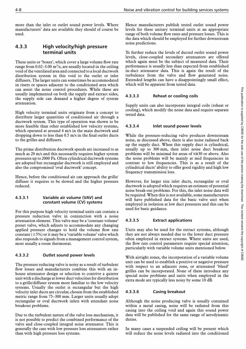
These units are placed around the perimeter of a room, typically under the windows, but if larger thermal duties are required they will often be formed into a continuous architectural unit with non-active sections. Some room occupants will usually be close to the units and this renders the direct sound level of primary importance to a specification, with little contribution from the room’s diffuse reverberant level.
Figures 4.6 and 4.7 indicate the basic operation principles and noise sources.
The primary air is forced through constrictive nozzles creating a local high velocity flow jet, which induces a greater volume (multiples of 5 are not uncommon) of secondary air. This noise source is very ‘hissy’ in its characteristic and leads to a fairly level noise power
spectrum from 500 up to 8 000 Hz. This is well screened from the room by the necessary front panel, which will be a feature of the supplier’s basic unit, see Figure 4.8 for a typical example. This hissy noise is therefore well directed upwards with a strong directivity pattern reducing the audible effect at 90° in front. Generally the induction ratio is highly affected by even modest back pressures, upstream or downstream, and noise attenuation is neither acceptable nor decoratively welcome. Thus the noise data are very
Acousticallining
Controlvalve
Balancingdamper
Roomthermostat
Primaryair supplyplenum
Inductionnozzles
Heatingcoil
Induced airenters frombottomand front
Figure 4.6 Induction type wall unit (reproduced courtesy of Weathermaker Equipment Ltd)
Noise radiatedfrom primaryair plenumchamber
Recirculationgrille
Inducedair
Panel radiatednoise fromstructure of unit
Jet noisefrom nozzles
Dischargegrille
Water return
Water supply
Air inlet
Figure 4.7 Sources of noise produced from induction unit (reproduced courtesy of SRL)
This publication is supplied by CIB
SE
for the sole use of the person making the dow
nload. The content remains the copyright of C
IBS
E.
Noise sources in building services 4-13
much determined by the initial selection remembering that the prime aim is a thermal performance.
The secondary induced airflow is quite slow in comparison as it spreads over the inlet cooling/heating coil(s) and will not be of acoustic concern.
Most units are supplied in tandem with cumulative air quantities flowing through an upper or lower plenum at a supply pressure necessary to push it to the last index unit. Balancing or take off dampers are incorporated at each unit to ensure the required distribution and these can produce noises at the lower end of the noise spectrum and to be derived from manufacturer’s data. Constant flow rate controllers can also be incorporated with their inherent noise generation characteristics, as they lower the supply duct pressure. These lower frequencies tend to be radiated from the front panel.
Generally the basic manufactured units are incorporated behind a decorative architectural feature, which will usually reduce this panel radiated noise to acceptable levels. Mock-ups will often be necessary to establish the overall noise performance often with direct sound pressure measurements rather than sound power levels.
As with other units discussed above, a pressure level measured at 1 m from the unit in an average room may well provide a reasonable sound power level assessment, preferable to data based on a diffuse field/reverberant room test.
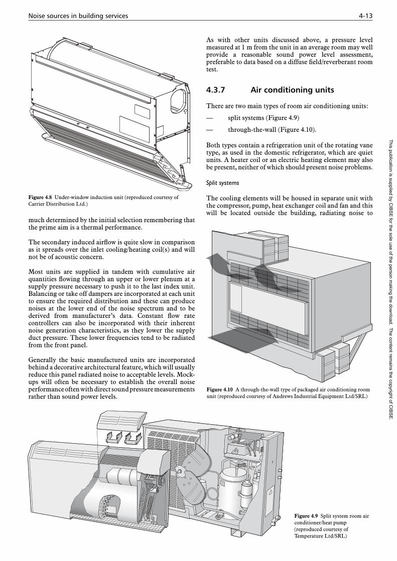
4.3.7 Air conditioning units
There are two main types of room air conditioning units:
— split systems (Figure 4.9)
— through-the-wall (Figure 4.10).
Both types contain a refrigeration unit of the rotating vane type, as used in the domestic refrigerator, which are quiet units. A heater coil or an electric heating element may also be present, neither of which should present noise problems.
Split systems
The cooling elements will be housed in separate unit with the compressor, pump, heat exchanger coil and fan and this will be located outside the building, radiating noise to
Figure 4.9 Split system room air conditioner/heat pump (reproduced courtesy of Temperature Ltd/SRL)
Figure 4.10 A through-the-wall type of packaged air conditioning room unit (reproduced courtesy of Andrews Industrial Equipment Ltd/SRL)
Figure 4.8 Under-window induction unit (reproduced courtesy of Carrier Distribution Ltd.)
This publication is supplied by CIB
SE
for the sole use of the person making the dow
nload. The content remains the copyright of C
IBS
E.
4-14 Noise and vibration control for building services systems
atmosphere. Its location relative to sensitive noise areas is therefore a consideration. Such situations include:
— lightwells
— openable windows, particularly those not benefiting from the conditioning
— residential areas where outdoor relaxation may be a daytime consideration.
The primary source of noise source is likely to be the cooling fan on the outside unit and the circulation fan on the room side perimeter or ceiling cassette unit. These will be catalogued as sound power levels for the exterior unit and sound power or pressure levels for the indoor conditioning unit.
The noise data for the room side unit will often be given as sound power levels from a diffuse field/reverberant room test on a supplier’s basic unit. When considering noise from a unit close to the occupant, care must be taken to consider the effect of directivity of the sound power propagating into a receiver position. The sound power spectrum will be essentially flat up to even 8 000 Hz but for perimeter units will be directed upwards. Hence, due to directivity at 90° for the occupant, these levels will contribute less of an audible sound pressure contribution to the direct sound field for the occupant. To this end, a sound pressure level measured at 1 m from the unit in an average room may well provide a more accurate assessment without any need to make further calculations. This is even more appropriate when a mock-up is required (see Real Room Acoustic Test Procedure (HEVAC, 1979)).
Further information on the interpretation of manufacturers’ literature can be found in Appendix 4.A3.
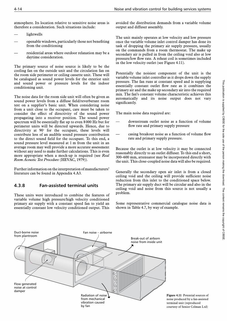
4.3.8 Fan-assisted terminal units
These units were introduced to combine the features of variable volume high pressure/high velocity conditioned primary air supply with a constant speed fan to yield an essentially constant low velocity conditioned output. This
avoided the distribution demands from a variable volume output and diffuser assembly.
The unit mainly operates at low velocity and low pressure once the variable volume inlet control damper has done its task of dropping the primary air supply pressure, usually on the commands from a room thermostat. The make up secondary air is pulled in from the ceiling void also at low pressure/low flow rate. A reheat coil is sometimes included in the low velocity outlet (see Figure 4.11).
Potentially the noisiest component of the unit is the variable volume inlet controller as it drops down the supply pressure. The fan runs at constant speed and is supplying essentially constant outlet flow rate as it combines the primary air and the make up secondary air into the required mix. The fan’s constant volume characteristic achieves this automatically and its noise output does not vary significantly.
The main noise data required are:
— downstream outlet noise as a function of volume flow rate and primary supply pressure
— casing breakout noise as a function of volume flow rate and primary supply pressure.
Because the outlet is at low velocity it may be connected reasonably directly to an outlet diffuser. To this end a short, 300–600 mm, attenuator may be incorporated directly with the unit. This close-coupled noise data will also be required.
Generally the secondary open air inlet is from a closed ceiling void and the ceiling will provide sufficient noise reduction from this inlet to the conditioned space below. The primary air supply duct will be circular and also in the ceiling void and noise from this source is not usually a problem.
Some representative commercial catalogue noise data is shown in Table 4.7, by way of example.
Duct-borne noisefrom plantroom
Flow generatednoise at controldamper
Break-out of airborn noise from inside unit
Fan noise – airborne
Radiation of noisefrom mechanicalvibration causedby fan
Figure 4.11 Potential sources of noise produced by a fan-assisted terminal unit (reproduced courtesy of Senior Colman Ltd)
This publication is supplied by CIB
SE
for the sole use of the person making the dow
nload. The content remains the copyright of C
IBS
E.

Noise sources in building services 4-15
Tab
le 4
.7(a
) F
an-a
ssis
ted
term
inal
uni
ts, s
ampl
e ac
oust
ic p
erfo
rman
ce d
ata,
Out
let L
W
Flo
wra
te
at 0
Pa
/ (L
/s)
Minimum operating pressure / Pa
125
Pa b
ox d
iffe
rent
ial p
ress
ure
250
Pa b
ox d
iffe
rent
ial p
ress
ure
500
Pa b
ox d
iffe
rent
ial p
ress
ure
Soun
d po
wer
leve
ls /
dB
at s
tate
d oc
tave
freq
uenc
y / H
zN
R*
Soun
d po
wer
leve
ls /
dB
at s
tate
d oc
tave
freq
uenc
y / H
zN
R*
Soun
d po
wer
leve
ls /
dB
at s
tate
d oc
tave
freq
uenc
y / H
zN
R*
Out
Pri
m63
125
250
500
1000
2000
4000
6312
525
050
010
0020
0040
0063
125
250
500
1000
2000
4000
125
125
1041
3933
2622
1516
1541
4034
2622
1516
1541
4135
2622
1517
16
145
125
1041
3934
3026
1916
1742
4035
3026
1916
1842
4036
3027
2017
18
145
145
1242
4035
3026
1916
1742
4136
3026
1916
1842
4238
3027
2017
19
175
125
1044
4237
3331
2921
2044
4238
3332
2921
2144
4239
3432
2921
21
175
145
1244
4238
3331
2921
2044
4339
3332
2921
2144
4340
3432
2921
21
175
175
1645
4339
3432
3022
215
4440
3432
3022
2144
4642
3532
2921
22
212
125
1047
4540
3534
3528
2548
4540
3535
3528
2549
4742
3635
3529
25
212
145
1247
4641
3634
3528
2548
4641
3635
3528
2549
4842
3735
3529
25
212
175
1647
4642
3734
3528
2548
4742
3735
3528
2549
4843
3735
3529
25
212
212
2047
4744
3835
3528
2548
4844
3835
3528
2549
4945
3835
3629
26
248
125
1050
5045
4038
3933
2951
5045
4039
3933
2952
5146
4139
3933
29
248
145
1250
5045
4038
3933
2951
5045
4139
3933
2952
5146
4139
3933
29
248
175
1650
5046
4138
3933
2951
5046
4139
3933
2952
5147
4139
3933
29
248
212
2050
5047
4139
3933
2951
5147
4139
3933
2952
5248
4239
3933
29
248
248
2550
5048
4239
3933
2951
5148
4239
3933
2952
5249
4239
3933
30
* D
esig
n re
verb
eran
t NR
val
ues
are
calc
ulat
ed u
sing
6 a
ir c
hang
es p
er h
our,
1 s
reve
rber
atio
n ti
me
(≤50
0 H
z) a
nd 0
.5 s
reve
rber
atio
n ti
me
(≥1
kHz)
This publication is supplied by CIB
SE
for the sole use of the person making the dow
nload. The content remains the copyright of C
IBS
E.

4-16 Noise and vibration control for building services systemsT
able
4.7
(b)
Fan
-ass
iste
d te
rmin
al u
nits
, sam
ple
acou
stic
per
form
ance
dat
a, B
reak
out L
W
Flo
wra
te a
t 0
Pa
/ (L
/s)
Minimum operating pressure / Pa
125
Pa b
ox d
iffe
rent
ial p
ress
ure
250
Pa b
ox d
iffe
rent
ial p
ress
ure
500
Pa b
ox d
iffe
rent
ial p
ress
ure
Soun
d po
wer
leve
ls /
dB
at s
tate
d oc
tave
freq
uenc
y / H
zN
R*
Soun
d po
wer
leve
ls /
dB
at s
tate
d oc
tave
freq
uenc
y / H
zN
R*
Soun
d po
wer
leve
ls /
dB
at s
tate
d oc
tave
freq
uenc
y / H
zN
R*
Out
Pri
m63
125
250
500
1000
2000
4000
6312
525
050
010
0020
0040
0063
125
250
500
1000
2000
4000
125
125
1052
4540
3430
3029
2452
4641
3530
3029
2452
4843
3730
3029
26
145
125
1053
4943
3633
3332
2653
4944
3733
3332
2653
5046
4033
3332
28
145
145
1253
4943
3633
3332
2653
4944
3733
3332
2653
5046
4033
3332
28
175
125
1054
5247
4039
4039
3254
5248
4139
4039
3254
5248
4239
4039
32
175
145I
1254
5248
4039
4039
3254
5249
4239
4039
3255
5249
4239
4039
32
175
175
1654
5249
4139
4039
3255
5250
4239
4039
3256
5452
4439
4039
34
212
125
1054
5350
4039
4039
3154
5350
4139
4039
3154
5350
4239
4039
31
212
145I
1255
5351
4139
4039
3255
5351
4239
4039
3555
5351
4339
4039
32
212
175
1655
5351
4239
4039
3255
5351
4339
4039
3255
5452
4440
4039
33
212
212
2056
5352
4341
4040
3356
5452
4441
4040
3357
5553
4541
4040
34
248
125
1057
5554
4745
4444
3658
5654
4746
4544
3658
5654
5047
4645
37
248
145I
1258
5655
4845
4444
3759
5755
4846
4544
3759
5755
5148
4645
38
248
175I
1658
5655
4846
4545
3759
5755
4847
4645
3760
5856
5148
4746
38
248
212I
2059
5756
4946
4545
3860
5856
4947
4645
3861
5957
5249
4746
39
248
248
2559
5756
4946
4545
3860
5856
4947
4645
3861
5957
5249
4746
39
* D
esig
n re
verb
eran
t NR
val
ues
are
calc
ulat
ed u
sing
6 a
ir c
hang
es p
er h
our,
1 s
reve
rber
atio
n ti
me
(≤50
0 H
z) a
nd 0
.5 s
reve
rber
atio
n ti
me
(≥1
kHz)
This publication is supplied by CIB
SE
for the sole use of the person making the dow
nload. The content remains the copyright of C
IBS
E.

Noise sources in building services 4-17
4.3.9 Rooftop units/air handling units
Rooftop plant is often not specifically designed as such, and may require extra protection or an advance schedule of noise and vibration control measures in order to complement the surrounding environment.
Sometimes the surroundings may change and will demand retrospective treatment to comply. An example would be the construction of a nearby but higher building whose façade is now exposed.
Roof top units tend to fall into two groups:
(a) Units conceived and dedicated as suitable for outdoor/roof top applications such as:
— cooling towers (dry air and water-cooled)
— condensing units
— air cooled chillers
— rooftop air handling units
— local extract and supply fan assemblies (e.g. kitchen extract, smoke extract)
— standby packages
— boiler flue outlets.
(b) Units that may well normally be sited indoors but now have a convenient roof top location such as:
— pumps
— boilers
— standby generators.
Each type is discussed in more detail below.
4.3.9.1 Cooling towers
Dry air cooling towers
If noise reduction is required, this has to allow for the free flow of the cooling air. This is most usually achieved by surrounding the unit with acoustic louvres at a suitable spacing. As a guide, the mid frequency nature of their traditional noise signature will enable such an array to offer about 10 dB of noise reduction by screening to adjacent locations. For applications that do not involve nearby high rise buildings the top can often remain open and unimpeded. If noise attenuation is deemed appropriate above the tower, then this will need to have a low pressure loss usually with comparatively long aerodynamic thin splitters.
If downward speed reductions are expected as a result of modulated duty changes, or for noise control purposes then care needs to be paid to the vibration isolation selection to ensure that resonance does not occur (see section 4.11).
Water-cooled cooling towers
Similar considerations as for dry air cooling towers apply, but airflow constraints are usually not too demanding.
4.3.9.2 Condensing units
Unless power assisted, when they become similar to the powered dry air cooling towers above, they are very quiet in the context of a rooftop plant area.
4.3.9.3 Rooftop air handling units
These units are very complex and may contain most of the components of a plant room to create a one-piece unitary assembly allowing it to be lifted into place in one go.
Generally a simple straight-line assembly is offered employing sections of matching cross section but bends and ‘L’ shapes may be contrived together with stacking.
Primarily they are an airtight thermally insulated enclosure and usually modular, meaning each section can be designed to meet an overall requirement with only the noisiest sections demanding specialist noise control features. These features may require thicker or mass loaded panels or even double panel constructions. The presence of thermal insulation usually takes the form of faced and protected mineral wool or fireproof foam, which offer well established acoustic noise control properties. Increasing the thickness of this lining can improve the noise reduction.
Typically the unit may contain:
— supply fan
— extract fan
— cooling coils
— fridge compressor units
— heating coils
— humidification unit
— heat recovery device
— filters
— boiler (gas or oil)
— pumps
— balancing dampers
— noise attenuators
— inlet and outlet grilles (with or without coupled dampers).
They may contain all of these items or just a fan assembly offering an airtight and convenient ducted inlet and outlet arrangement and insulation.
The prime noise sources are the supply fan and, if separate, the extract fan. In order not to propagate this noise level down the otherwise comparatively quiet complete assembly, noise attenuation is applied directly at the fan sections.
With axial flow fans both the inlet and outlet can incorporate close coupled cylindrical attenuators. However this often does not yield sufficient low frequency attenuation in a short enough length and transforms onto a splitter type attenuator are provided. This is often achieved by slipping the splitters directly into the air handler casing, with side linings being preferred to improve the casing breakout. To determine the noise breakout from the axial fan section, the breakout sound power level from the fan casing will be
This publication is supplied by CIB
SE
for the sole use of the person making the dow
nload. The content remains the copyright of C
IBS
E.

4-18 Noise and vibration control for building services systems
required. Generally only two-pole units require specialist attention.
With centrifugal fans the outlet is most usually transformed into a splitter type attenuator (as described for axial fans above). However, the inlet is usually drawn directly from the interior of its section. The air inlet into this section will be via a splitter type attenuator, similar to that of the outlet In many cases splitters will be slipped into the air handler standard airtight housing, again with side linings.
Hence this inlet plenum will be subject to the full inlet sound power level of the fan. Also, because the inlet conditions to the fan can be compromised by potentially cramped conditions, it is wise to confirm that the truly free inlet conditions of any test data will apply.
Predicting a guidance value for the sound power level radiated from this section of the unit is possible in a simple manner if the inside is acoustically/thermally lined. In this case a guidance value is obtained by subtracting the sound reduction index of the panel construction from the fan inlet sound power level, modified by any inlet condition modifications.
4.3.9.4 Fridge compressor units
Two main types of compressor are employed:
— reciprocating piston compressors
— rotary vane compressors.
Reciprocating piston compressors
These can be particularly noisy units, with annoyance potentially increased as a result of their intermittent on/off operation. Noise data must be sought, particularly as the noise will also propagate down the unit. They should be mounted on an inertia base with resilient mounts (selected according to the overall air handler unit vibration isolation or rails). It is recommended that such compressors should not be mounted within the air handling unit.
Rotary vane refrigerant compressors
Rotary vane refrigerant compressors are far less noisy, for the sizes likely to be within the air handling unit, even on start-up.
4.3.9.5 Boiler units (gas or oil)
Gas or oil boiler assemblies can be incorporated into air handlers and although the flame/heat exchanger will be within the panelled assembly, the powered burner itself is likely to be external, for access and maintenance.
Noise levels for these units, usually powered, will need to be established, especially any start-up peaks. This data should also be available in octave bands as any overall dBA ratings may be deceptive in that most of the acoustic power may be concentrated in the 125 Hz band.
The internal noise from the heat exchanger does not usually cause duct noise problems downstream from the unit.
4.3.9.6 Pumps
Pumps are not usually included within an air handling unit but if they are, should be selected to avoid them being a source of excessive airborne noise. This may require a simple protective and acoustic enclosure with consideration given to summer cooling, be it natural ventilation by a stack effect or powered and attenuated fan cooling.
Pumps should be mounted on an inertia base with resilient mounts selected with considerations to the roof span.
4.3.9.7 Balancing dampers
These dampers may be manual or motorised. If they are being employed for a modest degree of balancing between multiple outlets, then, because they are within the unit, break-out noise contributions above the other values is not expected.
Similarly, if they are employed via motorised units to modulate hot and cold air mixing, then break-out noise contributions above the other values is not expected.
4.3.9.8 Noise attenuators
The early section of these units is subject to the full fan noise level and due attention must be paid to this region. Side linings are recommended as a first measure of improved noise reduction. Because axial fans are usually transformed up to the attenuator within their section, this early attenuator region becomes subject to the full fan ducted noise level at the enclosures boundary. Two pole fans present the more common problems.
4.3.9.9 Inlet and outlet grilles with coupled dampers
Generally the return air inlet and conditioned supply air outlet will be ducted away to separate builders’ work openings and grilles.
Sometimes it is desired that any atmospheric inlet or outlet will include close coupled damper/grille arrangements. Interaction noise may be an unexpected problem when the turbulence of either item reacts on the adjacent component.
Sometimes the mixing requirements of partial fresh air to recirculation air can result in a mixing damper dropping appreciable pressure, leading to unpredicted noise at an outlet.
4.3.9.10 ‘Quiet sections’
The following sections may be considered as ‘quiet’ and not contributing to noise levels:
— cooling coils
— heating coils
— humidification unit
— heat recovery device
— filters
— inlet and outlet grilles without coupled dampers.
This publication is supplied by CIB
SE
for the sole use of the person making the dow
nload. The content remains the copyright of C
IBS
E.
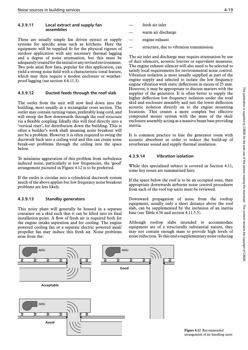
Noise sources in building services 4-19
4.3.9.11 Local extract and supply fan assemblies
These are usually simple fan driven extract or supply systems for specific areas such as kitchens. Here the equipment will be supplied fit for the physical rigours of outdoor application with any necessary thermal lagging and a degree of noise attenuation, but this must be adequately treated for the initial or any revised environment. Two pole axial flow fans, popular for this application, can yield a strong noise field with a characteristic tonal feature, which may then require a modest enclosure or weather-proof lagging (see section 4.6.11.3).
4.3.9.12 Ducted feeds through the roof slab
The outlet from the unit will now feed down into the building, most usually as a rectangular cross section. The outlet may contain turning vanes, preferably long cord, and will sweep the flow downwards through the roof structure via a flexible coupling. Ideally this will feed directly into a ‘vertical riser’, for distribution down the building. This is often a builder’s work shaft meaning noise breakout will not be a problem. However it is often required to swing the ductwork back into a ceiling void and this can create noise break-out problems through the ceiling into the space below.
To minimise aggravation of this problem from turbulence induced noise, particularly at low frequencies, the ‘good’ arrangement pictured in Figure 4.12 is to be preferred.
If the outlet is circular into a cylindrical ductwork system much of the above applies but low frequency noise breakout problems are less likely.
4.3.9.13 Standby generators
This noisy plant will generally be housed in a separate container on a skid such that it can be lifted into its final installation point. A flow of fresh air is required both for the engine intake aspiration and for cooling. The engine powered cooling fan or a separate electric powered axial/propeller fan may induce this fresh air. Noise problems arise from the:
— fresh air inlet
— warm air discharge
— engine exhaust
— structure, due to vibration transmission.
The air inlet and discharge may require attenuation by use of duct silencers, acoustic louvres or equivalent measures. The engine exhaust silencer will also need to be selected to satisfy local requirements for environmental noise control. Vibration isolation is most usually supplied as part of the engine supply and selected to isolate the low frequency engine vibration with static deflections in excess of 25 mm. However, it may be appropriate to discuss matters with the supplier of the generator. It is often better to supply the higher deflection low frequency isolation under the total skid and enclosure assembly and just the lower deflection acoustic isolation directly on to the engine mounting locations. This creates a more complex but effective compound mount system with the mass of the skid/enclosure assembly acting as a massive beam base providing inertia.
It is common practice to line the generator room with acoustic absorbent in order to reduce the build-up of reverberant sound and supply thermal insulation.
4.3.9.14 Vibration isolation
While this specialised subject is covered in Section 4.11, some key issues are summarised here.
If the space below the roof is to be an occupied zone, then appropriate downwards airborne noise control procedures from each of the roof top units must be reviewed.
Downward propagation of noise from the rooftop equipment, usually only a short distance above the roof slab, can be supplemented by the inclusion of an inertia base (see Table 4.56 and section 4.11.5.5).
Although rooftop slabs intended to accommodate equipment are of a structurally substantial nature, they may not contain enough mass to provide high levels of noise reduction. To this end a supplementary noise reducing
AHU AHU
AHU
Acceptable
Good
Avoid
Figure 4.12 Recommended arrangement of air handling units
This publication is supplied by CIB
SE
for the sole use of the person making the dow
nload. The content remains the copyright of C
IBS
E.
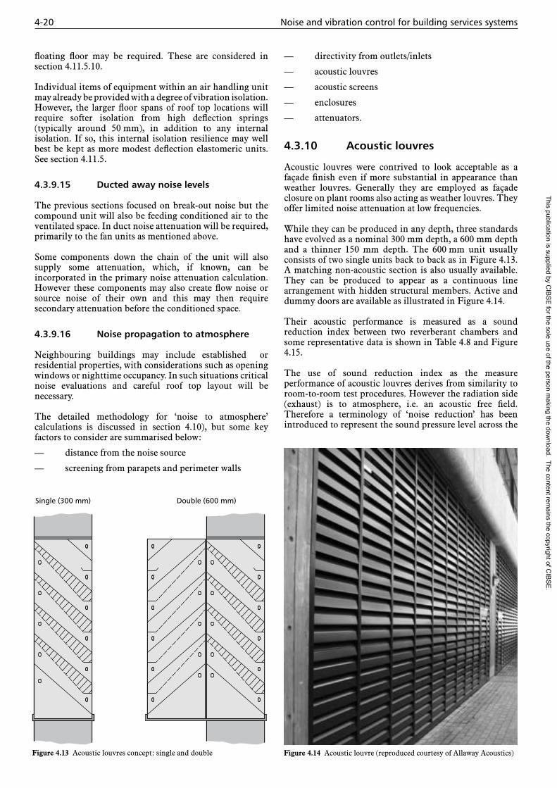
4-20 Noise and vibration control for building services systems
floating floor may be required. These are considered in section 4.11.5.10.
Individual items of equipment within an air handling unit may already be provided with a degree of vibration isolation. However, the larger floor spans of roof top locations will require softer isolation from high deflection springs (typically around 50 mm), in addition to any internal isolation. If so, this internal isolation resilience may well best be kept as more modest deflection elastomeric units. See section 4.11.5.
4.3.9.15 Ducted away noise levels
The previous sections focused on break-out noise but the compound unit will also be feeding conditioned air to the ventilated space. In duct noise attenuation will be required, primarily to the fan units as mentioned above.
Some components down the chain of the unit will also supply some attenuation, which, if known, can be incorporated in the primary noise attenuation calculation. However these components may also create flow noise or source noise of their own and this may then require secondary attenuation before the conditioned space.
4.3.9.16 Noise propagation to atmosphere
Neighbouring buildings may include established or residential properties, with considerations such as opening windows or nighttime occupancy. In such situations critical noise evaluations and careful roof top layout will be necessary.
The detailed methodology for ‘noise to atmosphere’ calculations is discussed in section 4.10), but some key factors to consider are summarised below:
— distance from the noise source
— screening from parapets and perimeter walls
— directivity from outlets/inlets
— acoustic louvres
— acoustic screens
— enclosures
— attenuators.
4.3.10 Acoustic louvres
Acoustic louvres were contrived to look acceptable as a façade finish even if more substantial in appearance than weather louvres. Generally they are employed as façade closure on plant rooms also acting as weather louvres. They offer limited noise attenuation at low frequencies.
While they can be produced in any depth, three standards have evolved as a nominal 300 mm depth, a 600 mm depth and a thinner 150 mm depth. The 600 mm unit usually consists of two single units back to back as in Figure 4.13. A matching non-acoustic section is also usually available. They can be produced to appear as a continuous line arrangement with hidden structural members. Active and dummy doors are available as illustrated in Figure 4.14.
Their acoustic performance is measured as a sound reduction index between two reverberant chambers and some representative data is shown in Table 4.8 and Figure 4.15.
The use of sound reduction index as the measure performance of acoustic louvres derives from similarity to room-to-room test procedures. However the radiation side (exhaust) is to atmosphere, i.e. an acoustic free field. Therefore a terminology of ‘noise reduction’ has been introduced to represent the sound pressure level across the
Single (300 mm) Double (600 mm)
Figure 4.13 Acoustic louvres concept: single and double Figure 4.14 Acoustic louvre (reproduced courtesy of Allaway Acoustics)
This publication is supplied by CIB
SE
for the sole use of the person making the dow
nload. The content remains the copyright of C
IBS
E.

Noise sources in building services 4-21
louvre from the reverberant side to 1 m on the atmospheric side. This is taken as the sound reduction index plus 6 dB.
Similarly the louvres are often employed directly at the end of ducts to atmosphere, inlet and exhaust. In this situation an insertion loss measurement would be desirable but is not usually available. The values for sound reduction index are usually employed but the performance attenuation achieved is likely to be less than this. This is particularly the case in the 63 Hz and 125 Hz bands due to the more normal incidence of the ducted sound wave in contrast to the values evaluated with reverberant room random incidence.
Frequently louvres are employed as acoustic and visual screens that allow a degree of airflow. Such applications include cooling towers and air handling units and many rooftop units of plant needing both a degree of noise reduction and to maintain atmospheric cooling. In these situations, the acoustic performance is best taken as an insertion loss equal to the sound reduction index and subtracted from any measured or predicted sound levels already established for the unscreened situation. The effects of diffraction of noise around any louvred screen may need to be considered.
The louvres offer a resistance to airflow, despite the blades being formed in an aerodynamic manner, and a representative pressure loss value for guidance would be 60 Pa at a face velocity of 2 m/s. Manufacturers’ data sheets should be consulted as unit configurations and performance vary depending on the acoustic demands.
4.3.11 Chillers and compressors
These produce both tonal and broadband noise. The tonal noise is typical of that from rotating or reciprocating
machinery, linked to the rotational frequency. The broad-band noise is from fluid flows, either liquid or gas. The tonal noise is often dominant, perceived as a whine or whirr, but the frequency range depends on the mode of operation. Reciprocating compressors have a relatively low-frequency fundamental tone, related to the oscillation frequency of the pistons. Screw compressors have strong tones in the octave bands between 250 and 2000 Hz, and may require special attention to noise and vibration control, especially when they are located externally.
The primary sources of noise are the compressors and drive motors. The following relations give the overall A-weighted sound pressure level (see Appendix 4.A2) at 1 m.
For centrifugal compressors:
LpA = 54 + 11 lg Pc (4.2)
For reciprocating compressors:
LpA = 66 + 9 lg Pc (4.3)
where LpA is the A-weighted sound pressure level at 1 m (dB) and Pc is the electrical power input to the compressor (kW).
See Table 4.13 (at the end of this section) for typical example noise levels, though use of manufacturers’ noise level data is always to be preferred.
4.3.12 Pumps
Pumps produce external noise from the motor, fluid-borne noise from the impeller and vibration into both the structure and the pipes. Noise problems may arise from the airborne noise, controlled by choosing a non-sensitive location or by an enclosure for the pump. If the pipes make solid contact with a radiating surface, there is the potential for both fluid-borne noise and pipe vibration to reappear as airborne noise at a distance from the pump. It is necessary to:
— use vibration isolators to isolate the pump from the building
— use a flexible connection from pump to pipes
— use resilient mountings for supporting the pipe to the structure.
See Table 4.13 (at the end of this section) for typical example noise levels.
4.3.13 Boilers
Hot water boilers may vary in size from less than a hundred kilowatts up to megawatts, depending on the heating requirement. Noise sources within the boiler room are from the air supply fan and the combustion. External noise is from the flue. A small boiler of about 200 kW capacity may have a spectrum peak at around 125 Hz and overall sound power level of 90 dBA. In general, the frequency of the peak drops with increasing boiler capacity so that, in the megawatt range, the spectrum peak is at 63 Hz or below. A large boiler, of several megawatt capacity, may have an overall sound power in excess of 100 dBA. Manufacturers’ information such as that shown in Table 4.9 below, should be consulted for octave band data as the presence of low
40
35
30
25
20
15
10
5
0
Soun
d re
duct
ion
inde
x
Frequency / Hz63 8k250125 500 1k 4k
Single acousticlouvre 300 mm
2k
Double acousticlouvre 600 mm
Figure 4.15 Acoustic louvre performance (single and double sound reduction index)
Table 4.8 Acoustic louvre performance
Type Sound reduction index / dB at stated octave frequency band / Hz
63 125 250 500 1000 2000 4000 8000
Single unit (300 mm)
5 5 7 12 18 21 16 16
Double unit (600 mm)
8 9 12 21 32 34 32 32
This publication is supplied by CIB
SE
for the sole use of the person making the dow
nload. The content remains the copyright of C
IBS
E.

4-22 Noise and vibration control for building services systems
frequencies leads to the A-weighted sound power level being an incomplete descriptor of the overall sound output of a boiler.
See Table 4.13 (page 4-30) for typical example noise levels.
4.3.14 Heat rejection and cooling towers
Cooling tower noise (see Figure 4.16) is mainly noise from the fan, details of which should be available from the manufacturer. Table 4.10, along with the correction factors given in Table 4.11, below, show typical sound power levels for cooling towers. See Table 4.13 (at the end of this section) for typical example sound pressure levels.
4.3.15 Chilled ceilings
Chilled ceilings fall into two main classes: passive units (beams and panels) and active units (powered by the supply air system).
4.3.15.1 Passive beams
These are simply long assemblies of finned water pipes located within the ceiling arrangement and their thermal action relies on the rising buoyant nature of the heated
Table 4.9 Boiler manufacturers’ typical data (reproduced courtesy of Hoval)
Boiler rating /kW dBA Unweighted sound pressure levels / dB at 1 m from burner at stated octave band / Hz
63 125 250 500 l000 2000 4000
30 50Generally these situations do not require acoustic treatment, even in domestic situations
50 6575 66 64 60 57 55 48 42 36
90 67 64 63 59 58 51 45 39125 69 67 66 65 61 56 47 43150 72 74 67 65 64 61 48 44
175 74 65 71 75 66 64 59 57200 70 67 71 73 66 68 60 58250 76 68 72 16 67 69 61 57
215 78 70 73 75 71 7? 63 62300 77 11 76 72 69 65 53 50400 75 73 73 70 66 62 54 14
500 77 74 78 77 73 54 59 55600 77 76 80 76 71 65 65 61800 77 74 79 77 71 61 64 59
900 82 80 86 80 79 68 65 611200 82 81 86 78 17 68 65 611500 82 82 87 77 74 68 66 60
1750 83 83 90 80 77 71 70 662000 83 83 90 80 77 71 70 662250 84 86 92 85 82 78 76 68
2750 85 87 92 88 86 86 78 723000 86 88 92 88 87 87 80 743500 88 93 98 90 87 86 84 78
4000 91 95 96 93 91 89 86 835000* 83 — — — — — — —6000* 81 — — — — — — —
Reduction for full acoustic shroud
15 8 13 20 24 28 30 28
Reduction for air inlet attenuators on models below 1500 kW
3 3 1 5 6 9 12 14
Note: accuracy = ±4dB. Use for oil, gas and dual fuel burners * Anticipated figure with fully enclosing acoustic shroud fitted
Figure 4.16 An example of the sound generated from a cooling tower
Waternoise
Fan noise
This publication is supplied by CIB
SE
for the sole use of the person making the dow
nload. The content remains the copyright of C
IBS
E.
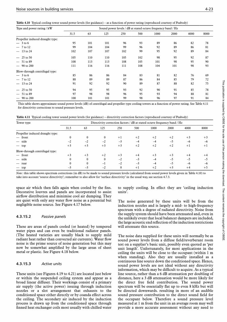
Noise sources in building services 4-23
space air which then falls again when cooled by the fins. Decorative louvres and panels are incorporated to assist airflow distribution and minimise cool air dumping. They are quiet with only any water flow noise as a potential but negligible noise source. See Figure 4.17 below.
4.3.15.2 Passive panels
These are areas of panels cooled (or heated) by tempered water pipes and can even be traditional radiator panels. (The heated varieties are usually black to supply mild radiant heat rather than convected air currents). Water flow noise is the prime source of noise generation but this may now be somewhat amplified by the large areas of sheet metal or plastic. See Figure 4.18 below.
4.3.15.3 Active units
These units (see Figures 4.19 to 4.21) are located just below or within the suspended ceiling system and appear as a broad linear diffuser. Their workings consist of a primary air supply (the active power) issuing through induction nozzles or a slot arrangement that exhausts to the conditioned space either directly or by coanda effect across the ceiling. The secondary air induced by the induction process is drawn up from the conditioned space through finned heat exchanger coils most usually with chilled water
to supply cooling. In effect they are ‘ceiling induction units’.
The noise generated by these units will be from the induction nozzles and is largely a mid- to high-frequency spectrum with a degree of radiated directivity. Noise from the supply system should have been attenuated and, even in the unlikely event that local balancer dampers are included, the large acoustic end reflection of the induction restrictions will attenuate this source.
The noise data supplied for these units will normally be as sound power levels from a diffuse field/reverberant room test on a supplier’s basic unit, possibly even quoted as ‘per unit length’. Unfortunately, for most applications in the ceiling the units will be close to the occupant (within 1 m when standing). Also they are usually installed as a continuous line source down the conditioned space. Hence, sound power levels are not ideal without any directivity information, which may be difficult to acquire. As a typical line source, rather than a 6 dB attenuation per doubling of distance, here a 3 dB attenuation would be more likely for the direct free field contribution. The sound power spectrum will be essentially flat up to even 8 kHz but will be directed downwards. resulting in more of an audible sound pressure contribution to the direct sound field for the occupant below. Therefore a sound pressure level measured at 1 m from the unit in an average room may well provide a more accurate assessment without any need to
Table 4.10 Typical cooling tower sound power levels (for guidance) – as a function of power rating (reproduced courtesy of Peabody)
Type and power rating / kW Sound power levels / dB at stated octave frequency band / Hz
31.5 63 125 250 500 1000 2000 4000 8000
Propeller induced draught type:— 3 to 6 95 101 101 96 93 89 86 82 78— 7 to 12 99 104 104 99 96 92 89 86 81— 13 to 24 102 107 107 102 99 95 92 89 84
— 25 to 50 105 110 110 105 102 98 95 92 87— 51 to 89 108 113 113 108 105 101 98 95 90— 90 to 200 111 116 116 111 108 104 101 98 93
Blow-through centrifugal type:— 3 to 6 85 86 86 84 83 81 82 76 69— 7 to 12 88 89 89 87 86 84 85 79 72— 13 to 24 91 92 92 90 89 87 88 82 75
— 25 to 50 94 95 95 93 92 90 91 85 78— 51 to 89 97 98 98 96 95 93 94 88 81— 90 to 200 100 101 101 99 98 96 97 91 84
This table shows approximate sound power levels (dB) of centrifugal and propeller type cooling towers as a function of power rating. See Table 4.11 for directivity corrections to sound pressure levels.
Table 4.11 Typical cooling tower sound power levels (for guidance) – directivity correction factors (reproduced courtesy of Peabody)
Tower type Directivity correction factors / dB at stated octave frequency band / Hz
31.5 63 125 250 500 1000 2000 4000 8000
Propeller induced draught type:— front 0 0 0 +1 +2 +2 +2 +3 +3— side –2 –2 –2 –3 –4 –4 –5 –6 –6— top +3 +3 +3 +3 +2 +2 +2 +1 +1
Blow-through centrifugal type:— front +3 +3 +2 +3 +4 +3 +3 +4 +4— side 0 0 0 –2 –3 –4 –5 –5 –5— rear 0 0 –1 –2 –3 –4 –5 –6 –6— top –3 –3 –2 0 +1 +2 +3 +4 +5
Note: this table shows spectrum corrections (in dB) to be made to sound pressure levels (calculated from sound power levels given in Table 4.10) to take into account ‘source directivity’; remember to also allow for ‘surface directivity’ in the usual way, see section 4.7.3.
This publication is supplied by CIB
SE
for the sole use of the person making the dow
nload. The content remains the copyright of C
IBS
E.

4-24 Noise and vibration control for building services systems
make further calculations. This is even more appropriate when a mock-up is required (see Real Room Acoustic Test Procedure, Appendix E (HEVAC, 1979)).
4.3.16 Lifts
The information below is mostly adapted from CIBSE Guide D: Transportation systems in buildings, sections 12.13.1 and 12.13.2 (2015a).
Criteria for in-car noise levels must take into account lift speed, as high-speed lifts are subject to wind noise. In-car noise criteria must also cover noise resulting from door operations. In hydraulic lifts, the oil flow can generate wide-band high frequency noise which is coupled to the lift
car via the cylinder. The addition of a silencer on the valve output can reduce this noise level in the car by up to 8 dBA.
Door noise, when measured at 1.5 m from the centre of the floor and 1.0 m from the door should not exceed 65 dBA. Noise levels in the car, when measured as above, should not exceed 55 dBA for lift speeds of 0.5–2.0 m/s and should not exceed 60 dBA for lift speeds of 2.0–7.0 m/s.
Lift noise, when measured at 1.5 m from the floor and 1.0 m from the door should generally not exceed 55 dBA at any
Cool air Hot airFigure 4.19 Active beam
Induced room air
Suspendedceiling
Primarycold air
Primaryair nozzles
Mixed supply air (coanda effect)
Primaryair plenum
Coolingcoil
Figure 4.20 Active beam
Figure 4.21 Photograph of an active beam
Warm, buoyant room air
Chilled air
Chilled air
Ceiling tile
Finned chilledwater pipes
Figure 4.17 Passive beam
Figure 4.18 Passive panel
This publication is supplied by CIB
SE
for the sole use of the person making the dow
nload. The content remains the copyright of C
IBS
E.

Noise sources in building services 4-25
time during the lift cycle. Where lifts open directly into office spaces (i.e. where there is no lift lobby), this limit should be reduced to 50 dBA.
However, there may be situations where levels up to 65 dBA may be acceptable and this should be checked with the client on each particular project.
The acceptable level of noise in lobbies will vary according to the function of the building. Noise ratings (NR values) for various areas within buildings are given in CIBSE Guide A (2015b). The recommended NR for reception areas in offices and hotel lobbies is NR35–40. For public areas in banks, building societies etc., NR35–45 is recommended. For circulation spaces between wards in hospitals, NR35 is recommended.
There are a number of different components of the lift which can generate noise including car door and lobby door closers; switches and contactors; rope noise, and the interaction of the guide rails and shoes or guide rollers.
Noise exposure limits in the lift machine room should be specified in accordance with the requirements of the Control of Noise at Work Regulations 2005 (TSO, 2005). It is therefore essential that levels of machine noise are obtained from the lift supplier.
It is also necessary to ensure that the sound reduction properties of the lift machine room construction (including doors, hatches, ventilation openings etc.) are adequate to prevent the escape of noise at values which exceed the acoustic design criteria for the surrounding areas.
Maximum noise levels shall be measured using a Class 1 sound level meter using the fast time weighting, and average noise levels shall be made over a complete cycle of lift operation. Noise levels in octave bands from 63–8000 Hz may also be required. The positions at which measurements are made should be noted on a drawing showing the principal noise-producing elements of the lift machinery. No measurements should be closer than one metre from any wall or floor surface. Further information on noise measurement is given in Appendix 4.A5 of this Guide.
4.3.16.1 Audible warnings and announcements
Lifts should be provided with an audible indication of their arrival at a landing, both in the car and on the landing. Voice synthesised announcements, of sufficient sound level to overcome background noise, should be included to announce door actions (opening and closing) as well as the floor level and direction of travel as the lift arrives at a landing.
Although voice annunciators are useful in situations where the lifts are regularly used by the general public or by blind or partially sighted people, they can also become a source of irritation to lift users. This can be avoided in part by enabling the volume to be adjusted between 35 and 55 dBA.
Emergency signals received from a fire alarm or building management system can also be announced by the voice synthesiser.
4.3.16.2 Vibration levels in lifts
Human response to vibration is greatest at low frequencies. Therefore vibration limits in the range 1–80 Hz should be specified. Furthermore, human susceptibility to vibration differs between horizontal and vertical vibration and this should be taken into account when specifying acceptable limits of vibration.
Vibration measurements should be made at the centre of the car, at floor level, in three mutually perpendicular axes corresponding to vertical, front-to-back and side-to-side. Measurements should be made of the vibration acceleration level in each direction over two complete cycles, one from the bottom of the building to the top, and one from the top of the building to the bottom. The measurement method is critical to the repeatability of results. It is, therefore, preferable to use an automatic recorder covering all fre-quency bands, as opposed to taking individual frequency band measurements over repeated lift runs. A cycle is defined as the period from just before the doors start to close at one level, to just after the doors open at the final level.
Acceleration levels should be measured as root mean square (Rms) values using a time weighting of 0.125 s (‘fast’), and the maximum values recorded in each ⅓-octave band from 1–80 Hz inclusive over each complete cycle. The following limits will apply:
(a) Horizontal vibration frequency range 1–80 Hz inclusive: maximum (Rms) acceleration level should not exceed 0.08 m/s2. The above limit applies to any time during a complete cycle, in any ⅓-octave band in the frequency range specified.
(b) Vertical vibration:
— At maximum speed: maximum (Rms) acceleration level in any ⅓-octave band should not exceed 0.08 m/s2 in the frequency range 1–80 Hz.
— During acceleration/deceleration and start/stop periods: the maximum (Rms) vibration acceleration level in any ⅓-octave band should not exceed 0.1 m/s2 in the frequency range 1–80 Hz.
The above limits apply to lifts with speeds up to 4 m/s.
Lifts having speeds above this will be subject to increased vibration limits. For lift speeds in the range 4–7 m/s, a multiplier of 1.5 may be used for all acceleration level limits.
Further information on vibration measurement is given in Appendix 4.A5 of this Guide. Criteria for acceptable levels of vibration in buildings arising from all types of building services equipment are given in CIBSE Guide A, chapter 1 (2015b).
4.3.17 Escalators
The following is adapted from CIBSE Guide D: Transportation systems in buildings, section 10.4.8 (2015a).
This publication is supplied by CIB
SE
for the sole use of the person making the dow
nload. The content remains the copyright of C
IBS
E.

4-26 Noise and vibration control for building services systems
Escalators are a source of noise and vibration from the motor and drive mechanism. This is not normally a problem provided that the equipment has been installed correctly, although no equipment can be totally silent or vibration-free in operation. The location of escalators or moving walks should be such as to cause minimum noise disturbance. If there is any doubt about the equipment then a similar installation should be checked. The design of the building is significant in noise and vibration reduction — for example, there is a possibility that vibration input from the motor will couple with a resonance on a surrounding floor or wall to produce a noticeable effect, which will then require correction. If the escalator or moving walk is required to operate to specific noise and vibration require-ments this should be agreed at the contract stage. Specialist advice may need to be sought.
4.3.18 Electric motors
Table 4.12 shows estimated sound pressure levels of electric motors at a distance of 1 m in a reverberant area, given as a function of power and speed. Note that these are typical levels to be used as guidance.
4.3.19 Noise from water flow systems
4.3.19.1 Sources of noise
Water based systems may include all water supply and wastewater systems.
Noise sources can include: pumps, water cooled chillers, cooling towers, cisterns, baths, taps and valves, washing machines and dishwashers. Some of these sources have been discussed earlier in this section.
4.3.19.2 Sound transmission paths
All the above sources will radiate airborne noise but in addition structure borne noise and water borne noise are important sound transmission paths in water flow systems.
Sound may be radiated by building elements (walls, floors etc.) as a result of structure borne excitation not only from structurally attached appliances (such as pumps, cisterns etc.) but also by water borne paths (e.g. by pipes). Therefore it is important that all equipment and appliances and pipework are effectively isolated from the building structure (see section 4.11 for more information).
4.3.19.3 Pumps and pipes
Pumps generate hydrodynamic noise particularly when turbulence occurs at the tip of impeller blades, and also noise from the pump motor and bearings. This will be a combination of broad band noise and tonal noise at the harmonics of the impeller blade passing frequency. The tonal component can be transmitted into the building structure as a result of water borne sound transmission and can cause annoyance, often as a humming sound. In order to minimise noise transmission, flexible connections should be fitted on the pump inlet and discharge. The pump may also need vibration isolation at support points.
Pump vibration may increase, together with associated noise emission, if the pump impeller becomes unbalanced due to dirt, sediment or wear. Excessive cavitation and air trapped in the system can also cause noise, so regular maintenance can reduce noise levels.
Additional noise may be generated by turbulent water flow in the pipes, which depends on factors such as water flow velocity, pipe diameter, and the smoothness of the water flow. Smoothness of flow depends on the pipework layout — i.e. the number of bends and fitting (valves etc.) — and the smoothness of the internal pipe walls, which can become uneven due to corrosion or build-up of impurities. For residential applications, valves attached to heating
Table 4.12 Estimated sound pressure levels of electric motors at a distance of 1 m (reproduced courtesy of Peabody)
Speed / (r/min) Power / kW Sound pressure level / dB at stated octave frequency band / Hz
31.5 63 125 250 500 1000 2000 4000 8000
Fast (2000–4000) <10 73 74 78 82 83 83 82 76 6910–20 78 79 83 87 88 88 87 81 7420–40 83 84 88 92 93 93 92 86 79
40–75 87 85 92 96 97 97 96 90 8375–150 90 91 95 99 100 100 99 93 86>150 93 94 98 102 103 103 102 96 89
Medium (1000–1999) <10 68 69 73 77 78 78 77 71 6410–20 73 74 78 82 83 83 82 76 6920–40 78 79 83 87 88 88 87 81 74
40–75 82 83 87 91 92 92 91 85 7875–150 85 86 90 94 95 95 94 88 81>150 88 89 93 97 98 98 97 91 84
Slow (450–999) <10 64 65 69 73 74 74 73 67 6010–20 69 70 74 78 79 79 78 72 6520–40 74 75 79 83 84 84 83 77 70
40–75 78 79 83 87 88 88 87 81 7475–150 81 82 86 90 91 91 90 84 77>150 84 85 89 93 94 94 93 87 80
This publication is supplied by CIB
SE
for the sole use of the person making the dow
nload. The content remains the copyright of C
IBS
E.

Noise control in plant rooms 4-27
radiators can generate noise which is transmitted to the radiator, from which the main sound radiation occurs. In industrial applications, pressure safety valves (psvs) and open vents can also produce significant noise if untreated. BS EN 60534-8-3 (BSI, 2011) provides detailed empirical formulae for predicting sound power levels generated through control valves under variable flow and material conditions. Pipe work can also be set into flexural (bending) vibration, with resonances occurring, depending on the size of the pipes and the distance between the pipe supports, dynamic stiffness of the pipe material, the pump speed and impeller blade passing frequency.
When pipes are passing through walls they are usually sleeved and should be isolated from the wall by suitable flexible materials. Any gap between pipe and sleeve is a potential path for airborne noise and should be packed when necessary. Direct contact between pipe and building structure will not only lead to structure borne transmission of pipe and pump noise but can also lead to intermittent noise (clicks, cracks, creaks etc.) arising from periodic expansion and contraction as temperatures change throughout the day and night.
Two specific noise generating mechanisms which can arise in water flow systems under certain conditions are cavitation and water hammer.
4.3.19.4 Cavitation
Cavitation is a phenomenon associated with the growth and collapse of vapour bubbles in a liquid. Cavities are formed and grow around small cavitation nuclei (very small solid particles or air bubbles) in the liquid when the liquid pressure is temporarily reduced to well below the liquid vapour pressure. These cavities subsequently collapse, violently, generating short bursts of very high pressure, and noise, when the liquid pressure returns to normal.
Cavitation may arise in pumps because the water pressure on one side of the impeller blade decreases at certain points in the rotation cycle. It should not occur under normal operating conditions, i.e. if the pump is operated in accordance with manufacturers’ instructions and is installed so that there are no obstacles to smooth streamlined water flow for several pump diameters upstream of the pump.
4.3.19.5 Water hammer
Water hammer is a repeated thumping or chattering noise which can occur when a tap or valve or stopcock is used to turn the water supply on or off suddenly. It occurs because the pressure wave that results and moves along the pipe from the sudden change in flow condition is reflected at a fitting such as a bend in the pipework or valve or tap. This causes a local increase in water pressure. There is therefore a sudden and transient increase of water pressure at the point of reflection, which gives rise to the noise.
Water hammer can occur if the flow rate is too high for the pipe size, or if the tap or valve is faulty (e.g. does not open or close cleanly), or if there are too many short sections of pipework close to the tap, or if the pipework is not secured firmly to the building structure.
Domestic equipment such as washing machines and dishwashers in flats and apartments can cause disturbance when automatic timers are used to operate late at night, and careful attention to isolation from building structure is required. Expansion vessels and other devices can be installed in pipework systems to minimise the effects of water hammer.
4.3.19.6 Waste water installations
Section 5.5.1 of BS EN 12354 (BSI, 2009a) gives the following useful summary:
‘A waste water installation is composed of any combination of straight pipes with tees, bends, joins and inlets, mounted on the building structures through fixing devices (often clips). Vibration is generated by the flow and fall of water in the piping system and either directly radiates sound (airborne sound) or is transmitted to the receiving structures (walls or floors to which the installation is fixed), which radiate sound (structure-borne sound); particular fixing devices can be used to reduce the structure-borne sound.’
In some cases, it may be necessary to acoustically lag pipework with an unfaced sound insulating material (e.g. mineral fibre) to minimise airborne noise propagating into sensitive areas. However, in some cases, it may not be practicable to do so. In such cases, it may be suitable to consider the fabrication material of the pipework. While there are a number of varying pipework materials available, (most notably plastic, cast iron and stainless steel) it is recommended that laboratory acoustic test data be carefully scrutinised from each manufacturer, preferably against a standardised test procedure, before an appropriate design decision can be reached. The current standardised test procedure for evaluating noise from waste water systems is BS EN 14366 (BSI, 2004a).
In summary, noise in water flow systems may be minimised by good choice of equipment, careful installation to ensure smooth water flow, avoidance of excessive flow velocities, isolation to prevent excitation of building structure, and good maintenance of equipment. BS EN 12354-5 (BSI, 2009a) gives information about predicting noise levels from some aspects of water flow noise.
4.4 Noise control in plant rooms
4.4.1 Risk of noise induced hearing loss
Exposure to high noise levels, such as may occur in a plant room, for extended periods of time can cause temporary or permanent hearing damage. Where employees are exposed to high noise levels at work, the Control of Noise at Work Regulations 2005 (TSO, 2005) imposes duties on employers, employees and on suppliers of equipment, depending on the level of noise exposure of employees. The noise level exposure of an employee is a combination of not only the sound levels to which the employee is exposed at work, but also the length of time for which he/she is exposed. The Regulations specify noise exposure action values and a noise exposure limit values. A summary of the Regulations is given below, for convenience, but the Regulations
This publication is supplied by CIB
SE
for the sole use of the person making the dow
nload. The content remains the copyright of C
IBS
E.

4-28 Noise and vibration control for building services systems
themselves should always be consulted to determine what must be done where employees, or others, are to be exposed to high levels of noise in plant rooms. HSE’s Controlling noise at work (HSE, 2005) provides useful information.
4.4.1.1 The Control of Noise at Work Regulations 2005
These Regulations (TSO, 2005) follow the requirements of EC Directive 2003/10 (EC, 2003). They replace the Noise at Work Regulations 1989, which had been in force since 1990.
Action and limit values
Lower exposure action value:
— personal daily (or weekly) noise exposure level of 80 dBA
— peak sound pressure level of 135 dBC.
Upper exposure action value:
— personal daily (or weekly) noise exposure level of 85 dBA
— peak sound pressure of 137 dBC.
Exposure limit value:
— personal daily (or weekly) noise exposure level of 87 dBA
— peak sound pressure level of 140 dBC.
In the Regulations, the various duties listed below are linked to employee noise exposure levels at or above the lower or upper exposure action values. However, the exposure limit values indicate an employee exposure level that the employer must not allow to be exceeded at the employee’s ear, when wearing hearing protectors.
Employers have a duty to:
— assess risks to employees
— reduce risks from noise as far as is reasonably practicable
— take action to reduce noise exposure
— provide employees with hearing protection
— make sure legal limits on noise exposure are not exceeded
— provide employees with information, instruction and training
— carry out health surveillance.
Employees have a duty to:
— comply with measures put in place by employers to reduce noise exposures
— inform management if any such measures including hearing protection) are in need of maintenance or replacement
— wear hearing protection when noise exposure levels are above the upper exposure action values.
Suppliers of equipment have a duty to:
— provide information about the noise emission of the equipment which they supply.
The Regulations require that even where noise exposure levels are below the lower action level noise exposure of employees should be reduced as far as is reasonably practicable, because high levels of noise can cause disturbance and impair working efficiency. Noise exposure levels may be reduced by reducing noise levels In the plant room, and/or by reducing times employees are exposed to high noise levels. Noise levels may be reduced by using quieter machinery, by reducing levels of reverberant sound (by use of sound absorbing material), by providing noise refuges within the plant room, or, as a last resort, by issuing hearing protectors, and ensuring that they are effective and used.
4.4.2 Breakout noise from plant rooms
Figure 4.3 in section 4.2 indicates how noise breaks out from plant rooms to adjacent occupied spaces and to atmosphere.
In order to reduce breakout noise the following steps must be taken:
— isolate the equipment from the structural floor, in order to minimise transmission of structure-borne noise
— ensure that the separating walls give sufficient attenuation
— ensure that all penetrations of the plant room walls, floor or ceiling are carefully sealed
— pay proper attention to noise transmission through the plant room external walls and silencing of air inlets and outlets, louvres etc. in order to control noise to atmosphere.
Isolation of equipment from plant room structure can be either by individual vibration isolation of each piece of equipment or by using a floating floor (see section 4.11 for further information).
Ensuring that the separating walls give sufficient attenuation requires information on the sound power outputs of each item of plant, so that the overall level and spectrum of the plant room noise can be estimated. The levels are then related to the noise criterion for the adjacent space and the requirements for wall attenuation determined. Many plant rooms have hard, sound reflecting walls, which contribute to the build-up of reverberant noise. This results in a higher internal level than might be anticipated, but the effect can be reduced by lining some of the plant room surfaces with (fire rated) sound absorbent materials. Reverberation must be included as a factor in predicting plant room noise levels. It may be necessary to design special noise attenuating double isolating walls to protect sensitive locations adjacent to plant rooms, and to make sure that pipes and other components are not fixed directly to these walls. These issues are discussed in sections 4.7 and 4.10 of this Guide.
Noise transmission from the plant room to the outside can be a potential cause of disturbance in neighbouring buildings and so should not be neglected in the design. In
This publication is supplied by CIB
SE
for the sole use of the person making the dow
nload. The content remains the copyright of C
IBS
E.
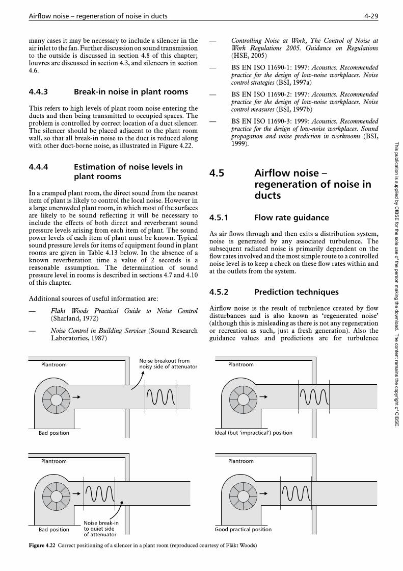
Airflow noise – regeneration of noise in ducts 4-29
many cases it may be necessary to include a silencer in the air inlet to the fan. Further discussion on sound transmission to the outside is discussed in section 4.8 of this chapter; louvres are discussed in section 4.3, and silencers in section 4.6.
4.4.3 Break-in noise in plant rooms
This refers to high levels of plant room noise entering the ducts and then being transmitted to occupied spaces. The problem is controlled by correct location of a duct silencer. The silencer should be placed adjacent to the plant room wall, so that all break-in noise to the duct is reduced along with other duct-borne noise, as illustrated in Figure 4.22.
4.4.4 Estimation of noise levels in plant rooms
In a cramped plant room, the direct sound from the nearest item of plant is likely to control the local noise. However in a large uncrowded plant room, in which most of the surfaces are likely to be sound reflecting it will be necessary to include the effects of both direct and reverberant sound pressure levels arising from each item of plant. The sound power levels of each item of plant must be known. Typical sound pressure levels for items of equipment found in plant rooms are given in Table 4.13 below. In the absence of a known reverberation time a value of 2 seconds is a reasonable assumption. The determination of sound pressure level in rooms is described in sections 4.7 and 4.10 of this chapter.
Additional sources of useful information are:
— Fläkt Woods Practical Guide to Noise Control (Sharland, 1972)
— Noise Control in Building Services (Sound Research Laboratories, 1987)
— Controlling Noise at Work, The Control of Noise at Work Regulations 2005. Guidance on Regulations (HSE, 2005)
— BS EN ISO 11690-1: 1997: Acoustics. Recommended practice for the design of low-noise workplaces. Noise control strategies (BSI, 1997a)
— BS EN ISO 11690-2: 1997: Acoustics. Recommended practice for the design of low-noise workplaces. Noise control measures (BSI, 1997b)
— BS EN ISO 11690-3: 1999: Acoustics. Recommended practice for the design of low-noise workplaces. Sound propagation and noise prediction in workrooms (BSI, 1999).
4.5 Airflow noise – regeneration of noise in ducts
4.5.1 Flow rate guidance
As air flows through and then exits a distribution system, noise is generated by any associated turbulence. The subsequent radiated noise is primarily dependent on the flow rates involved and the most simple route to a controlled noise level is to keep a check on these flow rates within and at the outlets from the system.
4.5.2 Prediction techniques
Airflow noise is the result of turbulence created by flow disturbances and is also known as ‘regenerated noise’ (although this is misleading as there is not any regeneration or recreation as such, just a fresh generation). Also the guidance values and predictions are for turbulence
Noise breakout fromnoisy side of attenuatorPlantroom
Bad position
Noise break-in to quiet side of attenuator
Plantroom
Bad position
Plantroom
Ideal (but ‘impractical’) position
Plantroom
Good practical position
Figure 4.22 Correct positioning of a silencer in a plant room (reproduced courtesy of Fläkt Woods)
This publication is supplied by CIB
SE
for the sole use of the person making the dow
nload. The content remains the copyright of C
IBS
E.

4-30 Noise and vibration control for building services systems
generated noise created from smooth incident flow conditions as indicated in Figure 4.26 (section 4.5.4).
When an already turbulent air stream is incident on a solid surface a new set of circumstances and noise data are created as illustrated in Figure 4.23. Hence, particular care is required when locating duct fittings close together because of the risk of turbulent interaction giving rise to higher than predicted airflow generated noise.
The generated sound power level from pressure loss obstructions in a duct system can be estimated from the following formula:
LW = C + 10 lg S + 60 lg u (4.4)
where LW is the airflow generated sound power level (dB), S is the minimum constrictive flow area of the fitting (m2) , u is the maximum flow velocity through the fitting (m/s) and C is a constant depending on the fitting description (some values are given in Table 4.14). This table generates octave band power levels but sometimes a pure tone is perceptible. This can usually be linked to the flow velocity, u (m/s) and a characteristic dimension, d (m), of an obstruction or constriction but also in resonance with some other duct feature. The approximate value for this frequency, f, will given by f = 0.2 u / d.
The formula also indicates the sensitivity of the flow noise to flow velocity as 18 dB per doubling of velocity (60 lg u). This signals that modest reductions in flow rate can yield useful 5 dB noise reductions. A more detailed determination of flow generated noise is given in Appendix 4.A2.
Table 4.13 Typical plant room noise levels for guidance (reproduced courtesy of Peabody)
Equipment Sound pressure levels / dB of mechanical equipment at 1 m at stated octave frequency / Hz
63 125 250 500 1000 2000 4000 8000
Chillers (100 tons+):— packaged reciprocating 90 89 92 93 92 90 86 81— packaged centrifugal 91 93 95 96 99 102 97 92— packaged screw 76 80 92 89 85 80 75 73
Boilers (40 kW+):— boilers 92 92 89 86 83 80 77 74— steam valve 70 70 70 75 80 85 90 95
Fans (up to 75 mm static pressure):— 20 kW 95 94 91 84 79 74 69 64— 40 kW 98 97 94 87 82 77 72 67— 75 kW 101 100 87 90 85 80 85 80— 200 kW 104 103 100 93 88 83 78 83
Fans (150 mm static pressure or over)— 40 kW 107 106 103 96 91 86 81 76— 75 kW 111 110 107 99 94 89 84 79— 200 kW 113 112 109 102 97 92 87 82
Cooling towers (intake noise):— centrifugal blow through 85 85 83 81 79 76 73 68— propeller induced draft 98 97 94 90 85 80 75 70
Pumps (1400 r/min):— 20 kW 83 86 90 90 86 83 80 75— 40 kW 86 89 93 93 89 86 83 78— 75 kW 89 92 96 96 92 89 86 81— 200 kW 92 95 99 99 95 92 98 84
Pumps (2800 r/min):— 20 kW 84 88 92 93 93 92 86 79— 40 kW 88 92 96 97 97 96 90 83— 75 kW 91 95 99 100 100 99 93 86
Air compressors (reciprocating and centrifugal):— 0.5 to 1.5 kW 83 83 83 86 89 89 89 84— 2 to 7 kW 86 86 86 89 92 92 92 87— 8 to 75 kW 89 89 89 92 95 95 95 90
Engines (internal combustion or diesel):— 20 kW 94 97 96 92 92 91 85 78— 40 kW 96 99 98 94 94 93 87 80— 75 kW 100 103 102 96 96 95 91 84— 200 kW 104 107 106 102 102 101 95 88— 400 kW 106 109 108 104 104 103 97 90— 750 kW 110 113 112 108 108 107 101 94— 2000 kW 114 117 116 112 112 111 105 98
This publication is supplied by CIB
SE
for the sole use of the person making the dow
nload. The content remains the copyright of C
IBS
E.

Airflow noise – regeneration of noise in ducts 4-31
To minimise flow generated noise and increase the chances of achieving both the guidance values given above and manufacturers’ performance data, the duct design should be as smooth as reasonable and not as shown in Figure 4.23. Some guide values for limiting duct velocities are given in Table 4.15 to control the level of flow generated noise to within specified room noise criteria.
4.5.2.1 Attenuators
While introduced into duct systems to reduce induct noise levels, they are also obstructions and generate flow noise, sometimes referred to as ‘regenerated’ or ‘self ’ noise.
Table 4.16 and Figure 4.24 give sample measured values for inlet and outlet flow generated noise for a splitter attenuator and clearly the inlet noise is greater than the outlet and will sound ‘hissy’. This can lead to unexpected noise experiences on extract systems were the attenuator inlet is facing the extract grille and being of a ‘hissy’ nature can be confused with similar sounding flow generated grille noise.
4.5.3 Damper noise
For guidance, Table 4.17 below illustrates some octave sound power levels for a range of single and double opposed blade damper sizes and duties.
However, wherever possible manufacturers’ data should be employed, as it will offer a larger range of performance data. Also it should be noted that nominally fully shut-off dampers may well produce high frequency whistles.
4.5.4 Turbulence-induced noise in and from ductwork
While turbulence in an airflow system cannot be avoided, it is not a continual problem that demands constant attention. However, it can cause issues and the guidance in this document is aimed at minimizing this risk.
4.5.4.1 Interaction between elements
Turbulent air discharging freely from the end of a duct at building services velocities below 20 m/s is generally acceptable, but if the duct is terminated with a grille much more noise will result. It is when the turbulence reacts with the surface of a following element that more major noise radiation results, and indeed this can be from the surface itself, e.g. the blades of a fan. It is primarily a function of airflow speeds and the simple guidance rule of 18 dB per doubling or halving of speed can be used as a rule of thumb. Hence, high velocity/high pressure distribution systems tend to carry the highest risks of unexpected problems for NR35 to NR40 situations but NR20 targets will always carry risks demanding more critical attention throughout the design and installation procedures.
Flow straighteners
A solution to this interaction between flow controlling elements, which can be applied to noisy combinations, is to introduce flow straighteners upstream of the second ‘interacted’ element, as shown in Figure 4.25. A length (L), which is 10 times the cell dimension (h), is often recommended to provide near perfect turbulence reduction, but in reality even a ratio of 1:1 can prove sufficiently useful to alleviate a problem to acceptable limits. To this end a
Fluctuating pressureon grille bladesradiated as noise
Turbulence
Figure 4.23 Noise generated by damper/grille combination (reproduced courtesy of Sound Research Laboratories)
Table 4.14 Corrections (C) to equation 4.3 for low turbulence duct fittings
Duct fitting Notes Value of C / dB
Octave band power level correction / dB for stated octave band / Hz
63 125 250 500 1000 2000 4000 8000
Straight duct No internal projections –10 0 –2 –7 –8 –10 –12 –15 –19
90° radiused bend Aspect ratio 2:1, throat radius w/2
0 0 –2 –7 –8 –10 –12 –15 –19
90° square bend with turning vanes
Close spaced, short radius single skin vanes
+10 0 –2 –7 –8 –10 –12 –15 –19
Gradual contraction Area ratio 3:1, A and u as for smaller duct
+1 0 0 –10 –16 –20 –22 –25 –30
Sudden contraction
Area ratio 3:1, A and u as for smaller duct
+4 +3 0 –10 –16 –20 –22 –25 –30
Butterfly damper
A and u apply to minimum free damper
–5 0 –3 –9 –9 –10 –17 –20 –24
This publication is supplied by CIB
SE
for the sole use of the person making the dow
nload. The content remains the copyright of C
IBS
E.

4-32 Noise and vibration control for building services systems
popular honeycomb construction known as ‘egg crate’ can be incorporated. If flow straighteners prove ineffective even at long lengths, then alternative solutions must be sought. Good and bad applications are illustrated in Figure 4.26 as part of the grille and diffuser takeoffs. They are also available as retrofitted options to reduce noise problems to acceptable limits.
The use of turning vanes in Figure 4.26 below serves to avoid the turbulence-exciting problem rather than solve it, but they would also act to reduce any turbulence already present in an approaching flow stream.
Further information on regenerated noise can be found in Appendix 4.A2.
4.5.4.2 Duct rumble
Another flow induced noise problem occurs with basic rectangular duct bends in tandem, often introduced to step round an obstruction in a ceiling void (see Figure 4.27 below). At high flow speeds duct buffeting and audible rumble may be generated.
A simplified and illustrative explanation is shown in Figure 4.28 below. As the turbulence swirls are in opposite directions the increased speeds at A, B, C etc. produce
h
L
Figure 4.25 Turbulence reduction by flow straighteners (left), rectangular ‘egg crate’ flow straightener (right)
Table 4.16 Self-generated noise for attenuator at 4 m/s face velocity
Flow LW per m2 of face area / dB at stated
octave band centre frequency / Hz
63 125 250 500 1000 2000 4000 8000
Inlet 45 55 58 66 68 65 59 49
Outlet 49 51 49 51 48 46 43 37
80
70
60
50
40
30
20
10
0
Soun
d po
wer
leve
l per
squa
re m
etre
of
face
are
a / d
B
Frequency / Hz63 8k250125 500 1k 4k
Outlet
2k
Inlet
Figure 4.24 Attenuator self generated flow noise at 4 m/s face velocity
Table 4.15 Suggested limiting duct velocities to restrict break-out of flow generated noise from grilles and ducts (reproduced courtesy of Sound Research Laboratories)
Duct type Rectangular Circular
Limiting duct velocity / (m/s) for stated NR
Limiting duct velocity / (m/s) for stated NR
20 25 30 35 20 25 30 35
Main ducts* (handling 50–100% of fan volume) 9.0 10.0 12.0 12.0 12.5 13.5 15.0 15.0
Main risers* (handling 10–70% of fan volume): — in builderswork masonry 7.5 7.5 8.5 10.0 9.0 11.0 13.0 15.0— in superficial timber or plasterboard voids 4.0 5.0 6.0 7.5 7.5 10.0 11.0 12.5
Run outs (handlinq 10–30% of fan volume)† 3.5 4.0 4.5 7.0 5.0 6.5 7.5 9.0
Feeder spurs† (handling <5% of fan volume) 2.5 3.0 3.5 4.5 3.5 4.0 5.0 6.0
Grille duct feeders: supply grilles (no dampers):— perfect uniform flow (1.42–0.47 m3/s) 1.5 1.8 2.1 2.5 1.5 1.8 2.1 2.5— perfect uniform flow (0.74–0.19 m3/s) 1.7 2.0 2.8 3.6 1.7 2.0 2.8 3.6— perfect uniform flow (<0.19 m3/s) 2.1 2.8 3.3 4.0 2.1 2.8 3.3 4.0— less good but not bad flow (i.e. normal situations) 1.2 1.5 1.7 2.5 1.2 1.5 1.7 2.5— bad flow N/a N/a 1.2 1.4 N/a N/a 1.2 1.4
Grille duct feeders: extract grilles (no dampers):— 1.42 to 0.47 m3/s 2.0 2.4 2.6 3.1 2.0 2.4 2.6 3.1— 0.74 to 0.19 m3/s 2.1 2.4 3.3 4.0 2.1 2.4 3.3 4.0— <0.19 m3/s 2.4 3.1 3.8 4.5 2.4 3.1 3.8 4.5
This table shows suggested limiting duct velocities to meet given NR levels in conditioned areas for various duct sections and configurations.
*Main ducts and main risers are not considered to be in the conditioned areas but only feeding to it. † Behind suspended ceiling of 12.5 mm mineral board tiles or better (not for open ceilings).
This publication is supplied by CIB
SE
for the sole use of the person making the dow
nload. The content remains the copyright of C
IBS
E.
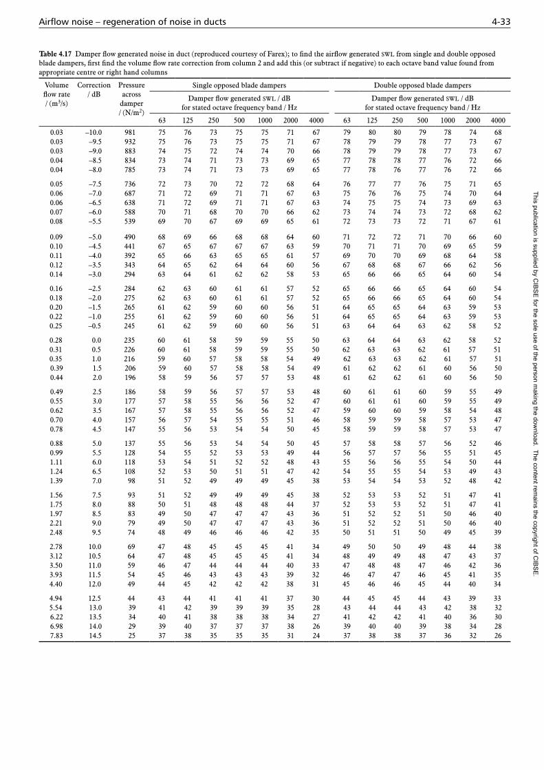
Airflow noise – regeneration of noise in ducts 4-33
Table 4.17 Damper flow generated noise in duct (reproduced courtesy of Farex); to find the airflow generated swl from single and double opposed blade dampers, first find the volume flow rate correction from column 2 and add this (or subtract if negative) to each octave band value found from appropriate centre or right hand columns
Volume flow rate / (m3/s)
Correction / dB
Pressure across
damper / (N/m2)
Single opposed blade dampers Double opposed blade dampers
Damper flow generated swl / dB for stated octave frequency band / Hz
Damper flow generated swl / dB for stated octave frequency band / Hz
63 125 250 500 1000 2000 4000 63 125 250 500 1000 2000 4000
0.03 –10.0 981 75 76 73 75 75 71 67 79 80 80 79 78 74 680.03 –9.5 932 75 76 73 75 75 71 67 78 79 79 78 77 73 670.03 –9.0 883 74 75 72 74 74 70 66 78 79 79 78 77 73 670.04 –8.5 834 73 74 71 73 73 69 65 77 78 78 77 76 72 660.04 –8.0 785 73 74 71 73 73 69 65 77 78 76 77 76 72 66
0.05 –7.5 736 72 73 70 72 72 68 64 76 77 77 76 75 71 650.06 –7.0 687 71 72 69 71 71 67 63 75 76 76 75 74 70 640.06 –6.5 638 71 72 69 71 71 67 63 74 75 75 74 73 69 630.07 –6.0 588 70 71 68 70 70 66 62 73 74 74 73 72 68 620.08 –5.5 539 69 70 67 69 69 65 61 72 73 73 72 71 67 61
0.09 –5.0 490 68 69 66 68 68 64 60 71 72 72 71 70 66 600.10 –4.5 441 67 65 67 67 67 63 59 70 71 71 70 69 65 590.11 –4.0 392 65 66 63 65 65 61 57 69 70 70 69 68 64 580.12 –3.5 343 64 65 62 64 64 60 56 67 68 68 67 66 62 560.14 –3.0 294 63 64 61 62 62 58 53 65 66 66 65 64 60 54
0.16 –2.5 284 62 63 60 61 61 57 52 65 66 66 65 64 60 540.18 –2.0 275 62 63 60 61 61 57 52 65 66 66 65 64 60 540.20 –1.5 265 61 62 59 60 60 56 51 64 65 65 64 63 59 530.22 –1.0 255 61 62 59 60 60 56 51 64 65 65 64 63 59 530.25 –0.5 245 61 62 59 60 60 56 51 63 64 64 63 62 58 52
0.28 0.0 235 60 61 58 59 59 55 50 63 64 64 63 62 58 520.31 0.5 226 60 61 58 59 59 55 50 62 63 63 62 61 57 510.35 1.0 216 59 60 57 58 58 54 49 62 63 63 62 61 57 510.39 1.5 206 59 60 57 58 58 54 49 61 62 62 61 60 56 500.44 2.0 196 58 59 56 57 57 53 48 61 62 62 61 60 56 50
0.49 2.5 186 58 59 56 57 57 53 48 60 61 61 60 59 55 490.55 3.0 177 57 58 55 56 56 52 47 60 61 61 60 59 55 490.62 3.5 167 57 58 55 56 56 52 47 59 60 60 59 58 54 480.70 4.0 157 56 57 54 55 55 51 46 58 59 59 58 57 53 470.78 4.5 147 55 56 53 54 54 50 45 58 59 59 58 57 53 47
0.88 5.0 137 55 56 53 54 54 50 45 57 58 58 57 56 52 460.99 5.5 128 54 55 52 53 53 49 44 56 57 57 56 55 51 451.11 6.0 118 53 54 51 52 52 48 43 55 56 56 55 54 50 441.24 6.5 108 52 53 50 51 51 47 42 54 55 55 54 53 49 431.39 7.0 98 51 52 49 49 49 45 38 53 54 54 53 52 48 42
1.56 7.5 93 51 52 49 49 49 45 38 52 53 53 52 51 47 411.75 8.0 88 50 51 48 48 48 44 37 52 53 53 52 51 47 411.97 8.5 83 49 50 47 47 47 43 36 51 52 52 51 50 46 402.21 9.0 79 49 50 47 47 47 43 36 51 52 52 51 50 46 402.48 9.5 74 48 49 46 46 46 42 35 50 51 51 50 49 45 39
2.78 10.0 69 47 48 45 45 45 41 34 49 50 50 49 48 44 383.12 10.5 64 47 48 45 45 45 41 34 48 49 49 48 47 43 373.50 11.0 59 46 47 44 44 44 40 33 47 48 48 47 46 42 363.93 11.5 54 45 46 43 43 43 39 32 46 47 47 46 45 41 354.40 12.0 49 44 45 42 42 42 38 31 45 46 46 45 44 40 34
4.94 12.5 44 43 44 41 41 41 37 30 44 45 45 44 43 39 335.54 13.0 39 41 42 39 39 39 35 28 43 44 44 43 42 38 326.22 13.5 34 40 41 38 38 38 34 27 41 42 42 41 40 36 306.98 14.0 29 39 40 37 37 37 38 26 39 40 40 39 38 34 287.83 14.5 25 37 38 35 35 35 31 24 37 38 38 37 36 32 26
This publication is supplied by CIB
SE
for the sole use of the person making the dow
nload. The content remains the copyright of C
IBS
E.

4-34 Noise and vibration control for building services systems
pressure minima and a pressure wave is produced, all travelling at the average flow rate. This could be as high as 20 m/s for a high velocity system. This moving pressure pattern will react with the duct walls and create buffeting. Corresponding low frequency rumble, will be generated together with harmonics from smaller vortex whirls.
Further to this the moving pattern hits the end wall of the next bend at right angles and reacts even more strongly. The proven solution is the simple introduction of plate splitters parallel to the airflow to break up the swirls in intensity and size, see Figure 4.29.
4.5.4.3 Turbulence reduction from control units: single blade dampers
When single blade dampers are operating in a substantial manner to reduce large upstream pressures, and are in a nearly closed position, the corresponding pressure drop will create large swirling vortices occupying most of the duct dimension (see Figure 4.30).
This can generate low frequency noise as above, especially if there is a high flow rate. In a clear run of duct, plates or honeycomb can be applied as before to reduce any noise levels down to specification. However, simple and cost effective single plate dampers, most often circular, will normally be fixed directly onto a proprietary conditioning unit meaning intermediate swirl reducers will not be possible. In this case the pressure reduction caused by the nearly closed blade must be lowered.
This can be achieved as a remedial process by the introduction of a perforated plate, selected from a range of percentage open areas as shown in Figure 4.31. The hole size should not be less than 4 mm to minimize the build up of dirt consistent with other features in the duct system, more especially extract systems. The pressure drop across the perforated plate will be associated with smaller turbulent swirls and associated mid frequency noise. The
High vel.low pressure
Flow
Pressureon centreline ofduct
Pressureat ductwall
High vel.low pressure
High vel.low pressure
X
A
X Z
Y Z
CBA
Y
B C
Figure 4.28 Duct buffeting
Full widthpartitionsor plates
Figure 4.29 Tandem bends duct buffering and rumble solution
Poordesign
Branch
Bend
Duct damper
Grille anddiffusertakeoffs
Gooddesign
Turningvanes
Figure 4.26 Examples of good and bad design for turbulence reduction
Figure 4.27 Tandem bends: duct buffering and rumble
This publication is supplied by CIB
SE
for the sole use of the person making the dow
nload. The content remains the copyright of C
IBS
E.
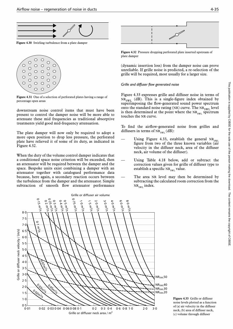
Airflow noise – regeneration of noise in ducts 4-35
downstream noise control items that must have been present to control the damper noise will be more able to attenuate these mid frequencies as traditional absorptive treatments yield good mid-frequency attenuation.
The plate damper will now only be required to adopt a more open position to drop less pressure, the perforated plate have relieved it of some of its duty, as indicated in Figure 4.32.
When the duty of the volume control damper indicates that a conditioned space noise criterion will be exceeded, then an attenuator will be required between the damper and the space. Bespoke units exist combining a damper with an attenuator together with catalogued performance data because, here again, a secondary reaction occurs between the turbulence from the damper and the attenuator. Simple subtraction of smooth flow attenuator performance
(dynamic insertion loss) from the damper noise can prove unreliable. If grille noise is predicted, a re-selection of the grille will be required, most usually for a larger size.
Grille and diffuser flow generated noise
Figure 4.33 expresses grille and diffuser noise in terms of NRswl (dB). This is a single-figure index obtained by superimposing the flow-generated sound power spectrum onto the standard noise rating (NR) curve. The NRswl level is then determined at the point where the NRswl spectrum touches the NR curve.
To find the airflow-generated noise from grilles and diffusers in terms of NRswl (dB):
— Using Figure 4.33, establish the general NRswl figure from two of the three known variables (air velocity in the diffuser neck, area of the diffuser neck, air volume of the diffuser).
— Using Table 4.18 below, add or subtract the correction values given for grille of diffuser type to establish a specific NRswl value.
— The area NR level may then be determined by subtracting the calculated room correction from the NRswl index.
Figure 4.30 Swirling turbulence from a plate damper
Figure 4.31 One of a selection of perforated plates having a range of percentage open areas
Figure 4.32 Pressure dropping perforated plate inserted upstream of plate damper
0·07m3/s
Gri
lle o
r di
ffus
er n
eck
velo
city
/ (m
/s)
Grille or diffuser air volume
NRSWL50
NRSWL40NRSWL30NRSWL20
Grille or diffuser neck area / m20·01 0·02 0·040·03 0·06 0·08 0·1 0·2 0·3 0·4 0·6 0·8 1·0 2·0 3·0
8·0
7·5
7·0
6·5
6·0
5·5
5·0
4·5
4·0
3·5
3·0
2·5
2·0
1·5
1·0
0·5
0·05m 3/s
0·03m 3/s0·02m 3/s
8·0 m3/s
6·0 m3/s
4·0 m3/s
3·0 m3/s
2·0 m3/s
1·5 m3/s
1·0 m3/s
0·75 m3/s
0·5 m3/s
0·4 m3/s
0·3 m3/s
0·25 m3/s
0·2 m3/s
0·15 m3/s
0·1 m3/s
Figure 4.33 Grille or diffuser noise levels plotted as a function of (a) air velocity in the diffuser neck, (b) area of diffuser neck, (c) volume through diffuser
This publication is supplied by CIB
SE
for the sole use of the person making the dow
nload. The content remains the copyright of C
IBS
E.
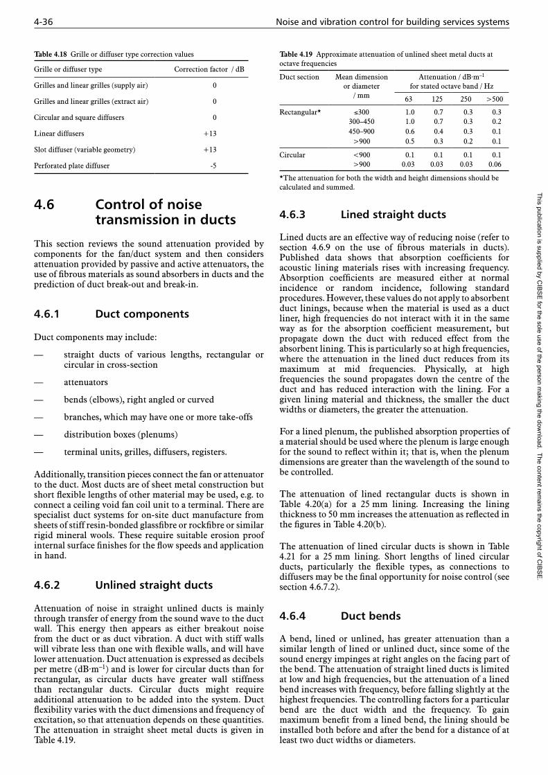
4-36 Noise and vibration control for building services systems
4.6 Control of noise transmission in ducts
This section reviews the sound attenuation provided by components for the fan/duct system and then considers attenuation provided by passive and active attenuators, the use of fibrous materials as sound absorbers in ducts and the prediction of duct break-out and break-in.
4.6.1 Duct components
Duct components may include:
— straight ducts of various lengths, rectangular or circular in cross-section
— attenuators
— bends (elbows), right angled or curved
— branches, which may have one or more take-offs
— distribution boxes (plenums)
— terminal units, grilles, diffusers, registers.
Additionally, transition pieces connect the fan or attenuator to the duct. Most ducts are of sheet metal construction but short flexible lengths of other material may be used, e.g. to connect a ceiling void fan coil unit to a terminal. There are specialist duct systems for on-site duct manufacture from sheets of stiff resin-bonded glassfibre or rockfibre or similar rigid mineral wools. These require suitable erosion proof internal surface finishes for the flow speeds and application in hand.
4.6.2 Unlined straight ducts
Attenuation of noise in straight unlined ducts is mainly through transfer of energy from the sound wave to the duct wall. This energy then appears as either breakout noise from the duct or as duct vibration. A duct with stiff walls will vibrate less than one with flexible walls, and will have lower attenuation. Duct attenuation is expressed as decibels per metre (dB·m–1) and is lower for circular ducts than for rectangular, as circular ducts have greater wall stiffness than rectangular ducts. Circular ducts might require additional attenuation to be added into the system. Duct flexibility varies with the duct dimensions and frequency of excitation, so that attenuation depends on these quantities. The attenuation in straight sheet metal ducts is given in Table 4.19.
4.6.3 Lined straight ducts
Lined ducts are an effective way of reducing noise (refer to section 4.6.9 on the use of fibrous materials in ducts). Published data shows that absorption coefficients for acoustic lining materials rises with increasing frequency. Absorption coefficients are measured either at normal incidence or random incidence, following standard procedures. However, these values do not apply to absorbent duct linings, because when the material is used as a duct liner, high frequencies do not interact with it in the same way as for the absorption coefficient measurement, but propagate down the duct with reduced effect from the absorbent lining. This is particularly so at high frequencies, where the attenuation in the lined duct reduces from its maximum at mid frequencies. Physically, at high frequencies the sound propagates down the centre of the duct and has reduced interaction with the lining. For a given lining material and thickness, the smaller the duct widths or diameters, the greater the attenuation.
For a lined plenum, the published absorption properties of a material should be used where the plenum is large enough for the sound to reflect within it; that is, when the plenum dimensions are greater than the wavelength of the sound to be controlled.
The attenuation of lined rectangular ducts is shown in Table 4.20(a) for a 25 mm lining. Increasing the lining thickness to 50 mm increases the attenuation as reflected in the figures in Table 4.20(b).
The attenuation of lined circular ducts is shown in Table 4.21 for a 25 mm lining. Short lengths of lined circular ducts, particularly the flexible types, as connections to diffusers may be the final opportunity for noise control (see section 4.6.7.2).
4.6.4 Duct bends
A bend, lined or unlined, has greater attenuation than a similar length of lined or unlined duct, since some of the sound energy impinges at right angles on the facing part of the bend. The attenuation of straight lined ducts is limited at low and high frequencies, but the attenuation of a lined bend increases with frequency, before falling slightly at the highest frequencies. The controlling factors for a particular bend are the duct width and the frequency. To gain maximum benefit from a lined bend, the lining should be installed both before and after the bend for a distance of at least two duct widths or diameters.
Table 4.19 Approximate attenuation of unlined sheet metal ducts at octave frequencies
Duct section Mean dimension or diameter
/ mm
Attenuation / dB·m–1 for stated octave band / Hz
63 125 250 >500
Rectangular* ≤300 1.0 0.7 0.3 0.3300–450 1.0 0.7 0.3 0.2450–900 0.6 0.4 0.3 0.1
>900 0.5 0.3 0.2 0.1
Circular <900 0.1 0.1 0.1 0.1>900 0.03 0.03 0.03 0.06
*The attenuation for both the width and height dimensions should be calculated and summed.
Table 4.18 Grille or diffuser type correction values
Grille or diffuser type Correction factor / dB
Grilles and linear grilles (supply air) 0
Grilles and linear grilles (extract air) 0
Circular and square diffusers 0
Linear diffusers +13
Slot diffuser (variable geometry) +13
Perforated plate diffuser -5
This publication is supplied by CIB
SE
for the sole use of the person making the dow
nload. The content remains the copyright of C
IBS
E.
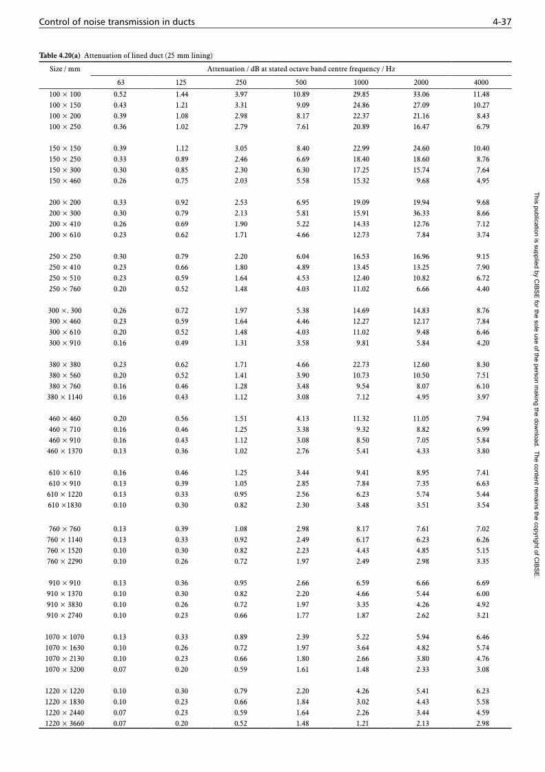
Control of noise transmission in ducts 4-37
Table 4.20(a) Attenuation of lined duct (25 mm lining)
Size / mm Attenuation / dB at stated octave band centre frequency / Hz
63 125 250 500 1000 2000 4000
100 × 100 0.52 1.44 3.97 10.89 29.85 33.06 11.48100 × 150 0.43 1.21 3.31 9.09 24.86 27.09 10.27100 × 200 0.39 1.08 2.98 8.17 22.37 21.16 8.43100 × 250 0.36 1.02 2.79 7.61 20.89 16.47 6.79
150 × 150 0.39 1.12 3.05 8.40 22.99 24.60 10.40150 × 250 0.33 0.89 2.46 6.69 18.40 18.60 8.76150 × 300 0.30 0.85 2.30 6.30 17.25 15.74 7.64150 × 460 0.26 0.75 2.03 5.58 15.32 9.68 4.95
200 × 200 0.33 0.92 2.53 6.95 19.09 19.94 9.68200 × 300 0.30 0.79 2.13 5.81 15.91 36.33 8.66200 × 410 0.26 0.69 1.90 5.22 14.33 12.76 7.12200 × 610 0.23 0.62 1.71 4.66 12.73 7.84 3.74
250 × 250 0.30 0.79 2.20 6.04 16.53 16.96 9.15250 × 410 0.23 0.66 1.80 4.89 13.45 13.25 7.90250 × 510 0.23 0.59 1.64 4.53 12.40 10.82 6.72250 × 760 0.20 0.52 1.48 4.03 11.02 6.66 4.40
300 ×. 300 0.26 0.72 1.97 5.38 14.69 14.83 8.76300 × 460 0.23 0.59 1.64 4.46 12.27 12.17 7.84300 × 610 0.20 0.52 1.48 4.03 11.02 9.48 6.46300 × 910 0.16 0.49 1.31 3.58 9.81 5.84 4.20
380 × 380 0.23 0.62 1.71 4.66 22.73 12.60 8.30380 × 560 0.20 0.52 1.41 3.90 10.73 10.50 7.51380 × 760 0.16 0.46 1.28 3.48 9.54 8.07 6.10
380 × 1140 0.16 0.43 1.12 3.08 7.12 4.95 3.97
460 × 460 0.20 0.56 1.51 4.13 11.32 11.05 7.94460 × 710 0.16 0.46 1.25 3.38 9.32 8.82 6.99460 × 910 0.16 0.43 1.12 3.08 8.50 7.05 5.84
460 × 1370 0.13 0.36 1.02 2.76 5.41 4.33 3.80
610 × 610 0.16 0.46 1.25 3.44 9.41 8.95 7.41610 × 910 0.13 0.39 1.05 2.85 7.84 7.35 6.63
610 × 1220 0.13 0.33 0.95 2.56 6.23 5.74 5.44610 ×1830 0.10 0.30 0.82 2.30 3.48 3.51 3.54
760 × 760 0.13 0.39 1.08 2.98 8.17 7.61 7.02760 × 1140 0.13 0.33 0.92 2.49 6.17 6.23 6.26760 × 1520 0.10 0.30 0.82 2.23 4.43 4.85 5.15760 × 2290 0.10 0.26 0.72 1.97 2.49 2.98 3.35
910 × 910 0.13 0.36 0.95 2.66 6.59 6.66 6.69910 × 1370 0.10 0.30 0.82 2.20 4.66 5.44 6.00910 × 3830 0.10 0.26 0.72 1.97 3.35 4.26 4.92910 × 2740 0.10 0.23 0.66 1.77 1.87 2.62 3.21
1070 × 1070 0.13 0.33 0.89 2.39 5.22 5.94 6.461070 × 1630 0.10 0.26 0.72 1.97 3.64 4.82 5.741070 × 2130 0.10 0.23 0.66 1.80 2.66 3.80 4.761070 × 3200 0.07 0.20 0.59 1.61 1.48 2.33 3.08
1220 × 1220 0.10 0.30 0.79 2.20 4.26 5.41 6.231220 × 1830 0.10 0.23 0.66 1.84 3.02 4.43 5.581220 × 2440 0.07 0.23 0.59 1.64 2.26 3.44 4.591220 × 3660 0.07 0.20 0.52 1.48 1.21 2.13 2.98
This publication is supplied by CIB
SE
for the sole use of the person making the dow
nload. The content remains the copyright of C
IBS
E.
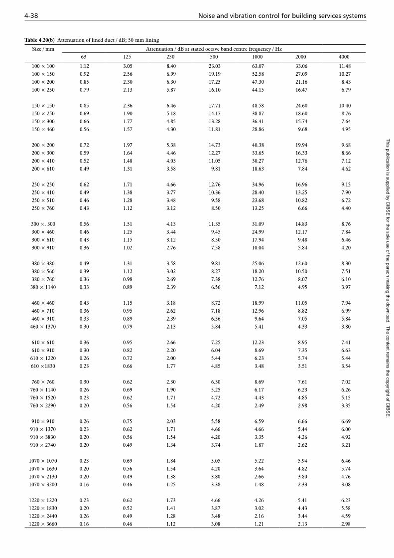
4-38 Noise and vibration control for building services systems
Table 4.20(b) Attenuation of lined duct / dB; 50 mm lining
Size / mm Attenuation / dB at stated octave band centre frequency / Hz63 125 250 500 1000 2000 4000
100 × 100 1.12 3.05 8.40 23.03 63.07 33.06 11.48100 × 150 0.92 2.56 6.99 19.19 52.58 27.09 10.27100 × 200 0.85 2.30 6.30 17.25 47.30 21.16 8.43100 × 250 0.79 2.13 5.87 16.10 44.15 16.47 6.79
150 × 150 0.85 2.36 6.46 17.71 48.58 24.60 10.40150 × 250 0.69 1.90 5.18 14.17 38.87 18.60 8.76150 × 300 0.66 1.77 4.85 13.28 36.41 15.74 7.64150 × 460 0.56 1.57 4.30 11.81 28.86 9.68 4.95
200 × 200 0.72 1.97 5.38 14.73 40.38 19.94 9.68200 × 300 0.59 1.64 4.46 12.27 33.65 16.33 8.66200 × 410 0.52 1.48 4.03 11.05 30.27 12.76 7.12200 × 610 0.49 1.31 3.58 9.81 18.63 7.84 4.62
250 × 250 0.62 1.71 4.66 12.76 34.96 16.96 9.15250 × 410 0.49 1.38 3.77 10.36 28.40 13.25 7.90250 × 510 0.46 1.28 3.48 9.58 23.68 10.82 6.72250 × 760 0.43 1.12 3.12 8.50 13.25 6.66 4.40
300 ×. 300 0.56 1.51 4.13 11.35 31.09 14.83 8.76300 × 460 0.46 1.25 3.44 9.45 24.99 12.17 7.84300 × 610 0.43 1.15 3.12 8.50 17.94 9.48 6.46300 × 910 0.36 1.02 2.76 7.58 10.04 5.84 4.20
380 × 380 0.49 1.31 3.58 9.81 25.06 12.60 8.30380 × 560 0.39 1.12 3.02 8.27 18.20 10.50 7.51380 × 760 0.36 0.98 2.69 7.38 12.76 8.07 6.10
380 × 1140 0.33 0.89 2.39 6.56 7.12 4.95 3.97
460 × 460 0.43 1.15 3.18 8.72 18.99 11.05 7.94460 × 710 0.36 0.95 2.62 7.18 12.96 8.82 6.99460 × 910 0.33 0.89 2.39 6.56 9.64 7.05 5.84
460 × 1370 0.30 0.79 2.13 5.84 5.41 4.33 3.80
610 × 610 0.36 0.95 2.66 7.25 12.23 8.95 7.41610 × 910 0.30 0.82 2.20 6.04 8.69 7.35 6.63
610 × 1220 0.26 0.72 2.00 5.44 6.23 5.74 5.44610 ×1830 0.23 0.66 1.77 4.85 3.48 3.51 3.54
760 × 760 0.30 0.62 2.30 6.30 8.69 7.61 7.02760 × 1140 0.26 0.69 1.90 5.25 6.17 6.23 6.26760 × 1520 0.23 0.62 1.71 4.72 4.43 4.85 5.15760 × 2290 0.20 0.56 1.54 4.20 2.49 2.98 3.35
910 × 910 0.26 0.75 2.03 5.58 6.59 6.66 6.69910 × 1370 0.23 0.62 1.71 4.66 4.66 5.44 6.00910 × 3830 0.20 0.56 1.54 4.20 3.35 4.26 4.92910 × 2740 0.20 0.49 1.34 3.74 1.87 2.62 3.21
1070 × 1070 0.23 0.69 1.84 5.05 5.22 5.94 6.461070 × 1630 0.20 0.56 1.54 4.20 3.64 4.82 5.741070 × 2130 0.20 0.49 1.38 3.80 2.66 3.80 4.761070 × 3200 0.16 0.46 1.25 3.38 1.48 2.33 3.08
1220 × 1220 0.23 0.62 1.73 4.66 4.26 5.41 6.231220 × 1830 0.20 0.52 1.41 3.87 3.02 4.43 5.581220 × 2440 0.26 0.49 1.28 3.48 2.16 3.44 4.591220 × 3660 0.16 0.46 1.12 3.08 1.21 2.13 2.98
This publication is supplied by CIB
SE
for the sole use of the person making the dow
nload. The content remains the copyright of C
IBS
E.
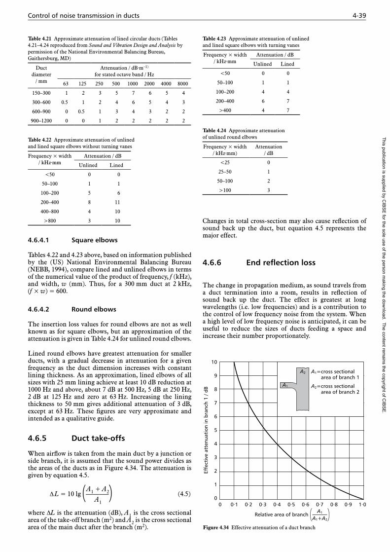
Control of noise transmission in ducts 4-39
4.6.4.1 Square elbows
Tables 4.22 and 4.23 above, based on information published by the (US) National Environmental Balancing Bureau (NEBB, 1994), compare lined and unlined elbows in terms of the numerical value of the product of frequency, f (kHz), and width, w (mm). Thus, for a 300 mm duct at 2 kHz, (f × w) = 600.
4.6.4.2 Round elbows
The insertion loss values for round elbows are not as well known as for square elbows, but an approximation of the attenuation is given in Table 4.24 for unlined round elbows.
Lined round elbows have greatest attenuation for smaller ducts, with a gradual decrease in attenuation for a given frequency as the duct dimension increases with constant lining thickness. As an approximation, lined elbows of all sizes with 25 mm lining achieve at least 10 dB reduction at 1000 Hz and above, about 7 dB at 500 Hz, 5 dB at 250 Hz, 2 dB at 125 Hz and zero at 63 Hz. Increasing the lining thickness to 50 mm gives additional attenuation of 3 dB, except at 63 Hz. These figures are very approximate and intended as a qualitative guide.
4.6.5 Duct take-offs
When airflow is taken from the main duct by a junction or side branch, it is assumed that the sound power divides as the areas of the ducts as in Figure 4.34. The attenuation is given by equation 4.5.
A1 + A2
Δ L = 10 lg (———–) (4.5) A1
where ΔL is the attenuation (dB), A1 is the cross sectional area of the take-off branch (m2) and A2 is the cross sectional area of the main duct after the branch (m2).
Changes in total cross-section may also cause reflection of sound back up the duct, but equation 4.5 represents the major effect.
4.6.6 End reflection loss
The change in propagation medium, as sound travels from a duct termination into a room, results in reflection of sound back up the duct. The effect is greatest at long wavelengths (i.e. low frequencies) and is a contribution to the control of low frequency noise from the system. When a high level of low frequency noise is anticipated, it can be useful to reduce the sizes of ducts feeding a space and increase their number proportionately.
Table 4.21 Approximate attenuation of lined circular ducts (Tables 4.21–4.24 reproduced from Sound and Vibration Design and Analysis by permission of the National Environmental Balancing Bureau, Gaithersburg, MD)
Duct diameter
/ mm
Attenuation / dB·m–1) for stated octave band / Hz
63 125 250 500 1000 2000 4000 8000
150–300 1 2 3 5 7 6 5 4
300–600 0.5 1 2 4 6 5 4 3
600–900 0 0.5 1 3 4 3 2 2
900–1200 0 0 1 2 2 2 2 2
Table 4.22 Approximate attenuation of unlined and lined square elbows without turning vanes
Frequency × width / kHz·mm
Attenuation / dB
Unlined Lined
<50 0 0
50–100 1 1
100–200 5 6
200–400 8 11
400–800 4 10
>800 3 10
Table 4.23 Approximate attenuation of unlined and lined square elbows with turning vanes
Frequency × width / kHz·mm
Attenuation / dB
Unlined Lined
<50 0 0
50–100 1 1
100–200 4 4
200–400 6 7
>400 4 7
Table 4.24 Approximate attenuation of unlined round elbows
Frequency × width / kHz·mm)
Attenuation / dB
<25 0
25–50 1
50–100 2
>100 3
1·00 0·1 0·2 0·3 0·4 0·5 0·6 0·7 0·8 0·9
10
9
8
7
6
5
4
3
2
1
0
Effe
ctiv
e at
tenu
atio
n in
bra
nch
1 / d
B
Relative area of branchA1
A1+A2
A1=cross sectional area of branch 1
A2=cross sectional area of branch 2
A1
A2
Figure 4.34 Effective attenuation of a duct branch
This publication is supplied by CIB
SE
for the sole use of the person making the dow
nload. The content remains the copyright of C
IBS
E.

4-40 Noise and vibration control for building services systems
The end reflection loss of a duct terminated flush with a wall is given as (NEBB, 1994):
Δ LR = 10 lg [1 + (0.8 λ / π d)1.88] (4.6)
where Δ LR is the reflection loss (dB), λ is the wavelength of the sound (m) and d is the diameter of a circular termination (m).
Wavelength is determined from c = λ f, see Appendix 4.A1. The effective diameter of a rectangular termination is:
d = √(4 A / π) (4.7)
where A is the area of the termination.
Equation 4.6 shows that the relation between wavelength and duct dimension (λ / d) is the controlling factor. The equation is to be used for end reflection losses for terminations having aspect ratios (i.e. height / width) of the order of unity. Slot diffusers were not investigated in the work which led to equation 4.6 and manufacturers’ data should be consulted for these components. Values of end reflection loss are given in Table 4.25.
When the duct terminates in ‘free space’, up to 3 dB can be added to these, see Table 4.26.
4.6.7 Passive attenuators and plenums
4.6.7.1 Passive or dissipative attenuators
A passive attenuator, see Figure 4.35, contains localized sound absorbent, normally associated with narrowed air passages. Both rectangular and circular attenuators are used. The rectangular attenuator is built up from an assembly of absorbent splitter modules. Its acoustic performance is determined largely by that of one of its single assemblies, which approximates to a narrow lined duct, known as a module. The parallel assemblies of these modules can be chosen to give an increased capacity to carry the required air volume without significant increase of velocity and pressure loss. The cross section of the attenuator is often significantly greater than that of the duct in which it is located. Changes in shape or cross section affect the operation of the attenuator. Attenuation and pressure loss increase as the airways are narrowed. Another important variable is the length of the attenuator. Longer attenuators have increased attenuation and some additional pressure loss. Attenuator pressure loss is not proportional to the length of the attenuator, since significant pressure loss occurs at the entry and exit. A circular attenuator is normally either open (‘una’) or contains an inner assembly, the absorbent ‘pod’ or ‘bullet’. Special systems may have concentric absorbent layers with airways between.
The static insertion loss of an attenuator is measured without airflow, usually employing noise from a loudspeaker. The dynamic insertion loss includes effects of airflow and will give modified results. While it may seem appropriate to employ the fan itself as the noise source as well as the airflow source this is not usually the case. There is a need to control each variable in an independent manner. However a most notable exception to this is the case for close-coupled cylindrical attenuators connected directly to the axial or mixed flow fan (see section 4.6.7.2).
The dynamic insertion loss is the insertion loss in the presence of flow and will be different for forward and reverse flow with respect to the direction of noise propagation (see Figure 4.36).
(a) (b)
(c)
Figure 4.35 Passive and dissipative duct attenuators; (a) rectangular, (b) circular, (c) rectangular elbow (reproduced from ASHRAE Handbook: HVAC Applications, by kind permission of ASHRAE)
Table 4.25 End reflection loss at octave band frequencies for flush mounting (reproduced from Sound and Vibration Design and Analysis by permission of the National Environmental Balancing Bureau, Gaithersburg, MD)
Duct dimension,
D / mm
End reflection loss / dB at stated octave band / Hz
63 125 250 500 1000
150 18 13 8 4 1
300 13 8 4 1 0
450 10 6 2 1 0
600 8 4 1 0 0
750 6 2 1 0 0
1000 5 2 1 0 0
1200 4 1 0 0 0
Table 4.26 End reflection loss at octave band frequencies for free space termination
Duct dimension,
D / mm
End reflection loss / dB at stated octave band / Hz
63 125 250 500 1000
150 21 16 11 7 3
300 16 11 7 5 1
450 13 9 5 4 0
600 11 7 4 3 0
750 9 5 3 2 0
1000 8 4 2 1 0
1200 7 3 1 0 0
‘Free space’ is considered to apply when the termination is greater than 1/10th wavelength of frequency band in question from a surface, e.g. 450 mm for 63 Hz band and shorter for all the higher bands.
This publication is supplied by CIB
SE
for the sole use of the person making the dow
nload. The content remains the copyright of C
IBS
E.

Control of noise transmission in ducts 4-41
Table 4.27 shows a comparison between a positive and negative face velocity with a range of ±10 m/s representing forward and reverse flow with respect to the noise propagation for a specific silencer. These are illustrative, based on a set of commercial tested data.
In building service applications an attenuator face velocity in excess of 6 m/s would be uncommon, once down the system away from the fan. As the variation is only in the region of 1 dB in the low frequency selection bands there is an understandable habit to ignore such dynamic insertion loss data.
In the mid frequency bands, where the corrections can be a little larger, the attenuations being offered are usually already in excess of requirements.
Flow generated noise occurs at both the inlet and outlet of an attenuator as a result of the momentum change as the air speeds up on airway entry and slows on exit. This flow noise is often incorrectly known or nicknamed as ‘regenerated noise’ as if noise has been reconstituted back into the system. This is not the case, as it is new noise, but the expression is likely to be encountered.
Some typical illustrative result sets for rectangular attenuators are shown in Figures 4.37 and 4.38 below for inlet and outlet flow generated noise power levels per square meter of duct cross section. They cover a face velocity range from 3 m/s to 10 m/s.
It will be noted that over most of the frequency band the inlet noise levels are greater than the outlet. It is often considered that the inlet level will be much less than the outlet as the inlet pressure loss (k) about 0.08, is less than that of the outlet, about 0.5. Early calculation methods often calculated the inlet flow noise as that of the outlet level attenuated by the attenuator’s insertion loss.
The tabulated content in Figures 4.37 and 4.38 is in traditional octave bands as consistent with this Guide. However ⅓-octave data is sometimes requested, as plotted in the graphs, due to the presence of a spectral peak. This peak indicates a characteristic nature to the noise which is ‘hissy’ rather than tonal and more prominent at lower flow rates. This may sometimes be confused with extract grille noise.
Due to presence of flow in any application, the concepts of ‘dynamic insertion loss’ and the noise generating aspect of ‘inlet and outlet flow generated noise’ have been introduced. Hence, when these corrections have been applied, the achieved loss of the attenuator will be modified, mainly by the airflow generation term rather than the dynamic insertion loss. Not surprisingly this is also incorrectly referred to as ‘the dynamic insertion loss’ when it is in fact ‘the effective dynamic insertion loss’. This should be considered.
Forward flow occurs when air and sound waves travel in the same direction, as in an air conditioning supply system or a fan discharge. Under forward flow conditions, high-frequency sound is refracted into the duct-silencer walls
Reverse flow occurs when sound waves and air travel in opposing directions, as in a typical return-air system. Under reverse flow conditions, sound is refracted away from the walls and toward the centre of the duct-silencer
Figure 4.36 Dynamic insertion loss illustrations (reproduced courtesy of IAC)
Table 4.27 Comparison of attenuator dynamic insertion losses / dB for forward and reverse flow
Face velocity (m/s)
Dynamic insertion losses / dB at stated octave band / Hz
63 125 250 500 1000 2000 4000 8000
+10 8 15 25 36 50 51 40 31 +8 9 16 26 37 50 51 39 30 +6 10 17 27 38 50 50 38 29
+3 11 18 28 39 50 50 37 28 0 11 18 28 40 50 50 37 27
–3 11 18 28 41 50 50 37 26
–6 12 19 29 42 50 50 36 25 –8 13 20 30 43 50 49 35 24
–10 14 21 31 44 50 49 34 23
This publication is supplied by CIB
SE
for the sole use of the person making the dow
nload. The content remains the copyright of C
IBS
E.

4-42 Noise and vibration control for building services systems
It must not be confused with the flow noise corrected application data (discussed below) which will alter again the ‘apparent nett attenuation’ for the installed unit.
Care must be taken in the location of attenuators in order to prevent interaction with other components. The attenuation values of two attenuators placed close together in series are not necessarily additive, since interactions and poor airflows may affect their operation.
Attenuators are included in the design when an analysis of the system has shown that the room criteria will not be met. The attenuation of passive attenuators is low at low frequencies, rises to a maximum in the middle frequencies (1–2 kHz) and drops at higher frequencies. Manufacturers’ attenuator data should be supported by a statement of the standards by which it was measured. Factors to be considered in selecting an attenuator include its attenuation at different frequencies and its pressure loss. Duct designs leading to poor entry and exit flow conditions increase the pressure loss and may generate additional low frequency noise. Particular attention should be given to the exit conditions.
It is advisable to locate attenuators several duct widths or diameters clear of bends, in order to maintain good airflow. Commercial packaged attenuators are available in a wide
range of configurations giving some control over dimen-sions, pressure loss and attenuation, in order to optimise the choice for a particular application. In general, higher attenuation is obtained by reducing the distance across the airway and by increasing the length of the attenuator. Pressure loss is reduced by increasing the airway area while keeping the cross dimension constant. That is, by either increasing the height of the attenuator or by adding additional airways to increase its width. Both these measures give a greater area for the airflow and so reduce the velocity in the airways, although too rapid a transition from a duct to an attenuator of greater cross-section than the duct, will not produce the full benefit. For a given airway, the pressure loss increases as the square of the air velocity and it is seen that, in specifying an attenuator, various requirements of insertion loss, pressure loss, space and cost must be balanced.
Location of an attenuator should be between the major noise source and the occupied space, preferably between straight duct runs in order to give good flow conditions at the entrance and exit to the attenuator. Often the major noise source is the plant room fan, but fan coil units, for example, introduce noise sources closer to the occupied space. A length of lined duct, between a ceiling void fan coil unit and the duct termination, may be adequate to deal with such fan coil unit noise.
80
70
60
50
40
30
20
10
0
1 /3-
octa
ve S
WL
per
squa
re m
eter
of
face
are
a /
dB
Frequency / Hz31·5 16 000250125 500 1000 80002000
Facevelocity /(m·s–1)
108643
63
58·055·050·544·540·5
125
61·558·053·046·541·5
250
64·561·056·550·045·5
Correction for face area, 10 × log (area)0·5–3
10
2+3
4+6
8+9
16+12
Area (m2):Correction:
500
Octave Lw per square metre of face area/ dB (re. 10–1 watts)
Inlet Lw
70·067·062·556·552·0
1000
69·566·562·556·552·5
2000
70·566·561·053·047·5
4000
69·564·056·546·039·0
800
64·557·047·533·523·5
4000
10
8
6
4
3
Figure 4.37 Indicative date for rectangular inlet flow generated noise
80
70
60
50
40
30
20
10
0
1 /3-
octa
ve S
WL
per
squa
re m
eter
of
face
are
a /d
B
Frequency / Hz31·5 16 000250125 500 1000 80002000
Facevelocity /(m·s–1)
108643
63
66·061·055·046·039·5
125
64·059·052·543·537·0
250
62·057·051·042·036·0
500
Octave Lw per square metre of face area/ dB (re. 10–1 watts)
Outlet Lw
65·560·053·043·036·0
1000
62·057·051·042·036·0
2000
64·058·050·540·032·5
4000
64·057·048·035·026·0
800
62·053·542·026·515·0
4000
10
8
6
4
3
Correction for face area, 10 × log (area)0·5–3
10
2+3
4+6
8+9
16+12
Area (m2):Correction:
Figure 4.38 Indicative date for rectangular outlet flow generated noise
This publication is supplied by CIB
SE
for the sole use of the person making the dow
nload. The content remains the copyright of C
IBS
E.

Control of noise transmission in ducts 4-43
Further information on the measurement of silencer acoustic performance can be found in BS EN ISO 7235 (BSI, 2009b).
4.6.7.2 Close coupled circular attenuators to axial/mixed flow fans
It is common and convenient to attach circular attenuators directly to the input and output flanges of axial and mixed flow fans (see Figure 4.39). These are well suited for the purpose, causing a minimum of disturbance to the fans natural installation mode. The pod or bullet designs, which offer higher performance, usually take in to account the blanking obstruction already present from the motor and the fan blades’ central support hub.
Figure 4.39 Podded cylindrical attenuator for direct attachment to axial fan outlet
The passage of air through the constricted airway would already be expected to generate flow noise, but since the air is spinning and progressing as a spiral or corkscrew the actual flow velocity is increased leading to greater flow noise than that expected by the average forward bulk flow rate. This is greater for high pitch angles, which spins the air off at a greater tangent. Furthermore, throttling the airflow from the duty pressures of application tightens the spiral and can affect airflow.
Hence ‘on fan’ data for the effectiveness of the close-coupled attenuator (outlet) is required from dedicated tests. A set of commercial catalogue test data is presented below in Table 4.28. It has become general practice to offer two standard lengths as one diameter long (1D), and two (2D). It should be noted that heating and ventilation fan diameters have become standardized now as metric ranges.
The unpodded design is unaffected by this spinning airflow in comparison to its modest insertion loss. However for the podded design the all-important mid-frequency dynamic losses are much reduced as the fan blade pitch angle is increased. This also renders the doubling in length a poor improvement at these mid-frequencies.
The low frequencies (long wavelengths) are not affected by this pitch angle effect.
Also, reduction of the delivered airflow volume by duct borne adjustments and features (in contrast to free flow conditions) does not affect these pitch effects because the air is still spinning but in a tighter spiral.
Comparisons of centrifugal and axial flow fans have shown an important contrast in their respective aerodynamic characteristics and the shape of the noise spectrum. Centrifugal fans are richer in low frequencies and axial fans are more peaky in the mid-frequency range. Hence the axial fan benefits from attenuation in these mid-frequency bands as is well illustrated by the close coupled data in Table 4.28.
4.6.7.3 Flexible circular duct attenuators
These units are primarily intended as secondary attenuators and are usually associated with the final run out to grilles and diffusers. They are available in a range of diametric sizes from 80 mm to 500 mm with a wall thickness of around 25 mm.
They offer cross-talk attenuation between rooms, primarily for the speech ranges, and also attenuation between balancing dampers and the grille. However they are not intended as solutions to major flow noise problems.
Table 4.29 offers some guidance data both with and without flow and when bent, in this case through 90°. In general terms the performance is not greatly affected by flow or bending. However they will generate their own flow noise, which may be of consequence for critical applications where the flow rates will need to be determined from separate data.
The guidance data is given as a substitution insertion loss for one metre and will include an acoustic entry and exit loss. Hence shorter lengths will give a marginally greater attenuation than that predicted by pro-rata length predictions and longer units will give marginally less.
Manufacturers` data and input should be sought for final calculations when the supplier is known. Care should be taken as the low frequency performance of flexible attenuators is derived principally from either casing breakout or end reflection effects, which may already have been accounted for elsewhere in calculations.
Care is also required when installing flexible duct attenuators to avoid constriction of the airway from bending.
4.6.7.4 Plenums
Plenums are analysed by considering the inlet duct as a source of sound power into the plenum. The sound reflects within the plenum, as in a room, and a proportion of the sound energy passes into the outlet duct. The factors to be considered are then the dimensions, relative positions of the inlet and outlet and the absorption coefficient of the plenum lining.
For the plenum shown in Figure 4.40 below, it can be shown that the insertion loss is given by:
(4.8)
where il is the insertion loss (dB), Aout is the outlet area of the plenum (m2), Q is a directivity factor depending on the location of the inlet (normally taken as 4 for plenums, see section 4.7.3), θ is the angle between the slant distance (r) and the plane containing the axis of the inlet duct (°), r is the slant distance from entry to exit (m), A is the total inside surface area minus the areas of the inlet and outlet (m2) and –a is the average absorption coefficient of the lining.
ILout
= + −
104
12
lgcos
AQ
r A
θ ααπ
This publication is supplied by CIB
SE
for the sole use of the person making the dow
nload. The content remains the copyright of C
IBS
E.

4-44 Noise and vibration control for building services systems
Equation 4.8 assumes that the wavelength of the sound is small compared with the dimensions of the plenum. That is, it assumes that sound in the plenum behaves like sound in a room. (Note: there are similarities between equation 4.8 for a plenum and equation 4.14 for a room.)
Equation 4.8 gives best results when the areas of the inlet and outlet are small compared with the total surface area. The positioning of the plenum may affect its performance, as duct lengths into and out of the plenum may resonate with components in the noise.
Table 4.28 Axial fan connected performance data: dynamic insertion loss (dB)
Fan diameter, D /mm
Attenuatorlength
Type ApproximateP/A setting
Dynamic insertion loss / dB for stated octave band centre frequency / Hz
63 125 250 500 1000 2000 4000 8000
300 1D Podded All 2 4 6 10 14 10 7 8
350 Unpodded Low 4 6 8 13 20 21 18 16
400 Medium 4 6 8 12 18 19 16 14
450 High 4 6 8 11 13 16 12 11
500 2D Podded Low 4 7 12 18 22 17 13 13
550 Medium 4 7 11 17 21 17 13 12
High 4 7 10 15 19 16 12 10
Unpodded Low 7 10 15 24 32 35 30 28
Medium 7 10 15 21 26 26 24 22
High 7 10 15 16 15 17 13 13
600 1D Podded All 3 4 8 14 14 9 8 7
650 Unpodded Low 4 6 9 17 26 21 18 12
700 Medium 4 6 9 17 23 20 18 11
800 High 4 6 9 16 17 16 14 11
2D Podded Low 6 8 14 23 24 15 13 10
Medium 6 8 13 22 22 14 13 9
High 6 8 12 20 18 13 11 9
Unpodded Low 8 11 16 30 39 35 32 22
Medium 8 11 16 27 32 32 29 19
High 8 11 16 24 23 23 24 17
1000 1D Podded All 3 4 9 14 12 8 7 7
1200 Unpodded Low 4 6 11 22 21 16 14 11
Medium 4 6 11 20 19 15 13 11
High 4 6 11 17 17 14 12 11
2D Podded Low 6. 8 14 22 20 13 12 10
Medium 6 8 13 21 18 12 11 10
High 6 8 12 19 15 11 10 9
Unpodded Low 8 11 19 30 32 30 24 17
Medium 8 11 19 26 27 26 22 17
High 8 11 19 21 20 22 20 16
1600 1D Podded All 4 5 10 14 11 7 6 6
1800 Unpodded Low 5 7 12 21 20 14 12 9
Medium 5 7 12 19 18 13 11 9
High 5 7 12 15 16 12 10 8
2D Podded Low 8 9 15 20 19 12 11 9
Medium 8 9 14 20 17 11 10 9
High 8 9 13 19 14 10 9 8
Unpodded Low 10 14 22 28 31 29 18 15
Medium 10 14 22 25 27 25 16 15
High 10 14 22 21 21 21 15 14
θ
r
Figure 4.40 Schematic of a plenum chamber
This publication is supplied by CIB
SE
for the sole use of the person making the dow
nload. The content remains the copyright of C
IBS
E.

Control of noise transmission in ducts 4-45
4.6.8 Active attenuators
Active attenuators detect the noise travelling in the duct and generate an opposing noise, of opposite phase, which is added to the travelling noise and results in cancellation. They are most effective in the low frequencies, where passive attenuators have limited performance.
There are two main configurations of active attenuator in which the active components are mounted either externally on the duct or in a central pod. The first type, illustrated in Figure 4.41(a), has some advantages for ease of retrofitting, while the second type, Figure 4.41(b), has technical advantages in the way in which the cancelling sound couples with the travelling sound. It also permits multiple units to be stacked to control noise in a large duct. Multiple units have been used, for example, to control noise breakout to atmosphere from air inlet or outlet openings. Active
attenuators have an application in natural ventilation, in order to give silenced, low pressure loss penetrations into the building.
Figure 4.41 shows how the upstream signal microphone picks up the travelling noise and sends it to a digital controller, which outputs the cancelling noise to the loudspeaker. The downstream control microphone supplies performance information back to the controller to modify its parameters, and minimise the remaining downstream noise. Absorptive material round the perimeter and in the pod controls high frequency noise, while the active components control lower frequency noise.
Active attenuators have developed well beyond the laboratory demonstration and are now produced commercially by several companies, generally in a hybrid configuration incorporating both passive and active
Table 4.29 Flexible circular duct attenuators performance data: sound attenuation with and without airflow
Duct type Flow Duct diameter / mm
Insertion loss / (dB/m) at stated octave band centre frequency / Hz
125 250 500 1000 2000 4000 8000
Straight flexible duct*
Zero 150 9 9 10 10 11 11 7
300 8 8 7 8 10 8 5
400 7 8 6 8 9 6 4
10 m/s 150 8 9 10 10 10 10 6
300 8 8 8 9 10 7 4
400 7 8 7 8 9 6 4
Flexible duct with 90° bends*
Zero 150 7 8 10 11 11 11 8
300 7 8 9 9 9 8 4
400 7 7 7 7 8 7 3
10 m/s 150 7 9 11 11 10 8 6
300 7 8 9 9 8 7 4
400 6 8 7 7 7 6 3
* Acoustic wall lining: 30 mm
(a)
(b)
Digitalcontroller
Signalmicrophone
Noise
Noise
Loudspeaker
Signal microphone Loudspeaker
Digital controller
Controlmicrophone
Controlmicrophone
Figure 4.41 Active attenuators; (a) mounted externally, (b) in a central pod
This publication is supplied by CIB
SE
for the sole use of the person making the dow
nload. The content remains the copyright of C
IBS
E.

4-46 Noise and vibration control for building services systems
absorption, which can give wide-band noise control. The main advantage of an active attenuator is that it gives good low frequency attenuation with lower pressure loss and in smaller space than an equivalent low frequency passive attenuator. There are a number of factors, such as air velocity, frequency range, duct dimensions, power supply continuity etc., which need to be considered in the selection of an active attenuator. Expert advice should be sought.
4.6.9 Use of fibrous sound absorbing materials in ducts
Although fibrous materials are excellent and inexpensive sound absorbers, there have been concerns over their use in ducts. Specifically, fibrous duct linings:
— may contribute to mould growth
— degrade with time
— erode from the surface and become carried in the air
— are difficult to clean.
In order to satisfy these concerns some general provisions that may be taken include the following:
— fibrous linings should be kept at least 3 m away from wet sections as mould growth may occur if they become wet
— care should be taken in the installation, especially to seal raw edges
— linings are available with toughened surfaces, treated for mould control
— in sensitive locations, the lining may be covered with a polyester (e.g. Mylar/Melinex™) film, although this reduces the absorption at high frequencies
— if the lining might be damaged it should be protected with a perforated metal or flattened expanded metal mesh sheet having at least 25% open area, in order to maintain the absorption properties of the lining material
— the material should be kept dry and undamaged prior to installation.
Unprotected fibrous material is sometimes used as a layer above suspended ceilings, for both noise control and thermal insulation. This results in a poor atmosphere for maintenance work above the ceiling and, if the ceiling tiles are moved, may result in fibres entering the space below.
4.6.10 Duct breakout noise
As duct materials are lightweight and thin, they transmit sound through the duct walls. This is known as breakout noise, which is a particular problem when long runs of duct pass over an occupied space. Breakout of noise leads to the noise in the duct reducing with distance, but breakout should never be used as a method of in-duct noise reduction unless the duct passes over non-sensitive spaces, such as storage areas. Break-in noise may also occur. For example, if the high noise level in a plant room breaks into a duct, the noise is then transmitted down the duct.
4.6.10.1 Rectangular sheet metal ductwork
Methods in previous editions of this CIBSE Guide have established a sound power or intensity level in the duct or more precisely, at an entrance to the duct and then applied duct wall sound reduction values to estimate the level of sound breaking out. This was rather like treating the duct as a long room and employed a sound reduction based on random incidence situations. In the duct, grazing incidence would be more appropriate when there is much more opportunity for grazing incidence ‘coincidence’ phenomena to occur and react with duct wall modes.
A serious issue with this method was that it could predict more power breaking out than had entered, as the level in the duct remained constant when in fact some of it had ‘broken out’ and been lost from the duct itself.
Both these are addressed in the method below where a separate ‘duct transmission loss’ is established and a sound level decay term is included as the sound travels down the duct but reduces at the same time due to breakout.
Having established the duct borne sound power level entering the duct at a zone entry point (LW,in) the total power level radiated to the zone is given by:
LW,out = LW,in – tlduct +10 lg L – (length effect)
(4.9)
The duct transmission loss (tlduct) depends on the frequency and the duct cross-section and is expressed here per 1 m unit of length. It must not be confused with the material’s basic sound reduction index, as determined in the familiar manner between two reverberant chambers and with random incidence noise. The terms here include an allowance for the ‘coincidence’ phenomena.
It is determined by experiment and a range of required frequency dependent values are given in Table 4.30 below for the popular steel duct thicknesses of 0.7 mm, 0.9 mm, 1.2 mm and 1.6 mm, which also includes the necessary cross sectional area allowance.
A degree of interpolation and extrapolation can be used remembering that this is guidance. Also notice that once the largest tabulated cross sections have been reached, the duct coincidence effect is absent and larger cross sections can be predicted noting that a 3 dB increase corresponds to a quadrupling (×4) of cross sectional area.
10 lg L is the length effect term where L is the exposed length to be considered in metres.
‘Length effect’ is the all-important additional duct length effect term that prevents over prediction for longer lengths and low ‘duct transmission loss’ values. The required values are presented in Figure 4.42. These basic steps are expanded as follows:
(1) Determine in-duct LW at point where duct enters the critical area. This will normally be due to a fan at some point in the duct system, to which will be applied the usual ductwork attenuation.
(2) Subtract duct transmission loss per unit length, as shown in Table 4.30, for appropriate duct wall
This publication is supplied by CIB
SE
for the sole use of the person making the dow
nload. The content remains the copyright of C
IBS
E.
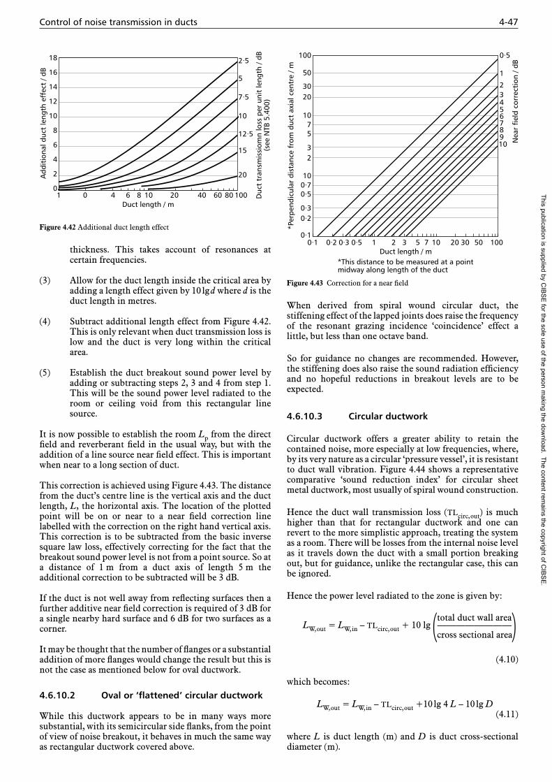
Control of noise transmission in ducts 4-47
thickness. This takes account of resonances at certain frequencies.
(3) Allow for the duct length inside the critical area by adding a length effect given by 10 lg d where d is the duct length in metres.
(4) Subtract additional length effect from Figure 4.42. This is only relevant when duct transmission loss is low and the duct is very long within the critical area.
(5) Establish the duct breakout sound power level by adding or subtracting steps 2, 3 and 4 from step 1. This will be the sound power level radiated to the room or ceiling void from this rectangular line source.
It is now possible to establish the room Lp from the direct field and reverberant field in the usual way, but with the addition of a line source near field effect. This is important when near to a long section of duct.
This correction is achieved using Figure 4.43. The distance from the duct’s centre line is the vertical axis and the duct length, L, the horizontal axis. The location of the plotted point will be on or near to a near field correction line labelled with the correction on the right hand vertical axis. This correction is to be subtracted from the basic inverse square law loss, effectively correcting for the fact that the breakout sound power level is not from a point source. So at a distance of 1 m from a duct axis of length 5 m the additional correction to be subtracted will be 3 dB.
If the duct is not well away from reflecting surfaces then a further additive near field correction is required of 3 dB for a single nearby hard surface and 6 dB for two surfaces as a corner.
It may be thought that the number of flanges or a substantial addition of more flanges would change the result but this is not the case as mentioned below for oval ductwork.
4.6.10.2 Oval or ‘flattened’ circular ductwork
While this ductwork appears to be in many ways more substantial, with its semicircular side flanks, from the point of view of noise breakout, it behaves in much the same way as rectangular ductwork covered above.
When derived from spiral wound circular duct, the stiffening effect of the lapped joints does raise the frequency of the resonant grazing incidence ‘coincidence’ effect a little, but less than one octave band.
So for guidance no changes are recommended. However, the stiffening does also raise the sound radiation efficiency and no hopeful reductions in breakout levels are to be expected.
4.6.10.3 Circular ductwork
Circular ductwork offers a greater ability to retain the contained noise, more especially at low frequencies, where, by its very nature as a circular ‘pressure vessel’, it is resistant to duct wall vibration. Figure 4.44 shows a representative comparative ‘sound reduction index’ for circular sheet metal ductwork, most usually of spiral wound construction.
Hence the duct wall transmission loss (tlcirc,out) is much higher than that for rectangular ductwork and one can revert to the more simplistic approach, treating the system as a room. There will be losses from the internal noise level as it travels down the duct with a small portion breaking out, but for guidance, unlike the rectangular case, this can be ignored.
Hence the power level radiated to the zone is given by:
total duct wall area LW,out = LW,in – tlcirc,out + 10 lg (————————) cross sectional area
(4.10)
which becomes:
LW,out = LW,in – tlcirc,out +10 lg 4 L – 10 lg D (4.11)
where L is duct length (m) and D is duct cross-sectional diameter (m).
18
16
14
12
10
8
6
4
2
0
Add
itio
nal d
uct
leng
th e
ffec
t / d
B
Duc
t tr
ansm
issi
omn
loss
per
uni
t le
ngth
/ dB
(see
NTB
5.4
00)
Duct length / m1 0 4 6 8 10 20 40 60 80 100
2·5
5
7·5
10
12·5
15
20
Figure 4.42 Additional duct length effect
Duct length / m*This distance to be measured at a pointmidway along length of the duct
1005020 301 2 3 5 7 100·50·20·1 0·3
100
50
3020
1075
32
100·70·5
0·30·2
0·1
*Per
pend
icul
ar d
ista
nce
from
duc
t ax
ial c
entr
e / m
Nea
r fie
ld c
orre
ctio
n / d
B
0·5
1
2345678910
Figure 4.43 Correction for a near field
This publication is supplied by CIB
SE
for the sole use of the person making the dow
nload. The content remains the copyright of C
IBS
E.

4-48 Noise and vibration control for building services systems
Guidance values of tlcirc,out for circular ducts for use in equation 4.11 are given in Table 4.31.
4.6.11 Duct break-in noise
4.6.11.1 Noise break-in
Initially the duct will be assumed to be in a uniform reverberant sound pressure field from an activity in the space across which the duct runs, e.g. a plant room or a
noisy function room. This reverberant sound pressure level is, splin.
The formula for determining the level of sound power leaving either end of the duct due to noise pick-up or break-in is:
LW,out = splin – tlin + 10 lg S (4.12)
where LW,out is the sound power level (dB) leaving either end of the duct and independent of airflow direction and in addition to any sound power levels from other sources.
Table 4.30 Breakout transmission loss per unit length for rectangular ducts
Steel duct thickness
/ mm
Duct cross section / mm
Breakout transmission loss, tlrect, out (/ dB), at stated octave band centre frequency / Hz
63 125 250 500 1000 2000 4000
0.7 (22 swg)
150 × 150 15 10* 16 17 20 23 27150 × 300 11* 11* 17 18 21 24 28150 × 600 12* 12* 18 19 22 25 29
300 × 300 13* 18 19 20 23 26 30300 × 600 14* 19 20 21 24 27 31
300 × 1200 15* 20 21 22 25 28 32
600 × 600 21 21 22 23 26 29 33600 × 1200 22 22 23 24 27 30 34600 × 1800 23 23 24 25 28 31 35
1200 × 1200 24 24 25 26 29 32 361200 × 1800 25 25 26 27 30 33 37
0.9 (20 swg)
150 × 150 16 16 12* 18 21 24 28150 × 300 12* 17 13* 19 22 25 29150 × 600 18 18 14* 20 23 26 30
300 × 300 14* 19 20 21 24 27 31300 × 600 15* 20 21 22 25 28 32
300 × 1200 16* 21 22 23 26 29 33
600 × 600 22 22 23 24 27 30 34600 × 1200 23 23 24 25 28 31 35600 × 1800 24 24 25 26 29 32 36
1200 × 1200 25 25 26 27 30 33 371200 × 1800 26 26 27 28 31 34 38
1.2 (18 swg)
150 × 150 18 18 14* 20 23 26 30150 × 300 14* 19 15* 21 24 27 31150 × 600 20 20 16* 22 25 28 32
300 × 300 16* 21 22 23 26 29 33300 × 600 17* 22 23 24 27 30 34
300 × 1200 18* 23 24 25 28 31 35
600 × 600 24 24 25 26 29 32 36600 × 1200 25 25 26 27 30 33 37600 × 1800 26 26 27 28 31 34 38
1200 × 1200 27 27 28 29 32 35 391200 × 1800 28 28 29 30 33 36 40
1.6 (16 swg)
150 × 150 20 20 16* 22 25 28 32150 × 300 21 16 17* 23 26 29 33150 × 600 22 22 18* 24 27 30 34
300 × 300 23 18* 24 25 28 31 35300 × 600 19* 19* 25 26 29 32 36
300 × 1200 25 20* 26 27 30 33 37
600 × 600 21 26 27 28 31 34 38600 × 1200 22 27 28 29 32 35 39600 × 1800 23 28 29 30 33 36 40
1200 × 1200 29 29 30 31 34 37 411200 × 1800 30 30 31 32 35 38 42
* Duct resonance occurs here
This publication is supplied by CIB
SE
for the sole use of the person making the dow
nload. The content remains the copyright of C
IBS
E.

Control of noise transmission in ducts 4-49
splin is the reverberant sound pressure level incident on the duct wall (dB). tlin is the break-in transmission loss of the duct (dB), depending on rectangular or circular cross section and size as given for guidance in Table 4.33, where S is the cross-sectional area of the duct (m2).
The complex sound pressure field in the duct will establish a balance between the inflow of the uniform break-in energy and the breakout loss. The measured tlin values represent a balance between the external reverberant pressure field and the internal sound pressure level.
4.6.11.2 Location of ductwork
Generally, ductwork will be close to the ceiling slab above and possibly also a nearby sidewall as if tucked away in a corner rather than hanging freely in a uniform reverberant field. Unfortunately these locations lead to increases in the sound pressure levels at low frequencies/long wavelengths. Hence increased level corrections are suggested as summarised in Table 4.32.
Guidance tlin values for rectangular and circular ducts are provided in Tables 4.33 and 4.34 (below) respectively.
Table 4.31 Breakout transmission loss per unit length for circular ducts
Steel duct thickness
/ mm
Diameter / mm
Breakout transmission loss, tlcirc, out (/ dB), at stated octave band centre frequency / Hz
63 125 250 500 1000 2000 4000 8000
0.7 (22 swg)
100 50 50 50 50 48 38 38 41
200 50 49 45 39 34 33 38 41
300 44 39 34 29 28 33 38 41
600 36 29 24 23 29 33 38 41
1500 26 22 21 23 29 33 38 410.9
(20 swg)100 50 50 50 50 49 40 39 40
200 50 50 46 41 36 35 39 40
300 47 42 36 31 30 35 39 40
600 37 32 27 26 30 35 39 40
1500 28 24 23 26 30 35 39 401.2
(18 swg)100 50 50 50 50 50 42 42 41
200 50 50 50 49 38 37 42 41
300 50 46 40 34 34 37 42 41
600 41 35 30 30 34 37 42 41
1500 32 27 26 30 34 37 42 411.5
(16 swg)100 50 50 50 50 50 43 42 40
200 50 50 50 50 40 39 42 40
300 50 46 41 35 35 39 42 40
600 42 37 32 31 35 39 42 40
1500 33 28 27 31 35 39 42 40
Table 4.32 Sound pressure level corrections for different duct locations
Octave band / Hz
Sound pressure level corrections /dB at stated location
Adjacent to ceiling slab above
In a corner
63 +3 +6
125 +2 +4
250 +1 +2
50
40
30
20
10
0
Soun
d re
duct
ion
inde
x /
dB
Frequency / Hz63 8000250125 500 1000 40002000
Stiffnesscontrol
Masscontrol
Coincidenceplateau
Figure 4.44 Representative comparative ‘sound reduction index’ for circular sheet metal ductwork
This publication is supplied by CIB
SE
for the sole use of the person making the dow
nload. The content remains the copyright of C
IBS
E.

4-50 Noise and vibration control for building services systems
4.6.11.3 Noise reduction: lagging/cladding
When a piece of sheet metal equipment, such as a ceiling void terminal unit or fan coil unit, produces more than an acceptable amount of casing noise radiation, then one noise reduction technique is to clad or lag or ‘wrap up’ the item in a material such as mineral wool.
Table 4.35 below indicates some guidance of the noise reduction that can be obtained from well-established basic lagging materials from the mineral fibre range. The wrapping process must be continuous and thorough in its
application as any exposed areas will generally have a disproportional detrimental effect on the achievable reduction. These applications will also add considerable thermal insulation, which, while this is often a desirable add-on, may also deter an inherent and required cooling effect.
The first seven rows in Table 4.35 are for completely basic material without any outer secondary barrier or protection. In reality if a protection is required it should be of a very light and flexible material if the tabulated data is to be realized. The traditional crinkly foil employed by the
Table 4.33 Break-in transmission loss for rectangular ducts
Steel duct thickness
/ mm
Duct cross section / mm
Break-in transmission loss, tlrect, in (/ dB), at stated octave band centre frequency / Hz
63 125 250 500 1000 2000 4000 8000
0.7 (22 swg)
150 × 150 17 17 17 23 32 37 40 42150 × 300 16 16 16 24 32 35 39 42150 × 600 15 15 16 27 30 33 39 42
300 × 300 14 14 17 26 31 34 39 42300 × 600 13 13 18 26 29 33 39 42
300 × 1200 12 12 21 24 27 33 39 42
600 × 600 11 11 20 25 28 33 39 42600 × 1200 10 12 20 23 27 33 39 42600 × 1800 9 16 19 22 27 33 39 42
1200 × 1200 8 14 19 22 27 33 39 421200 × 1800 7 15 18 21 27 33 39 42
0.9 (20 swg)
150 × 150 17 17 17 25 34 39 42 42150 × 300 16 16 17 26 35 38 41 42150 × 600 15 15 18 29 32 35 41 42
300 × 300 14 14 19 28 33 36 41 42300 × 600 13 13 20 29 32 35 41 42
300 × 1200 12 12 23 26 29 35 41 42
600 × 600 11 13 22 27 30 35 41 42600 × 1200 10 14 23 26 29 35 41 42600 × 1800 9 18 21 24 29 35 41 42
1200 × 1200 8 16 21 24 29 35 41 421200 × 1800 8 17 20 23 29 35 41 42
1.2 (18 swg)
150 × 150 17 17 19 28 37 42 42 42150 × 300 16 16 20 29 37 40 42 42150 × 600 15 15 21 32 35 38 42 42
300 × 300 14 14 22 31 36 39 42 42300 × 600 13 14 23 31 34 38 42 42
300 × 1200 12 15 26 29 32 38 42 42
600 × 600 11 16 25 30 33 38 42 42600 × 1200 10 17 25 28 32 38 42 42600 × 1800 9 21 24 27 32 38 42 42
1200 × 1200 10 19 24 27 32 38 42 421200 × 1800 10 20 23 26 32 38 42 42
1.6 (16 swg)
150 × 150 17 17 21 30 39 42 42 42150 × 300 16 16 22 31 40 42 42 42150 × 600 15 15 23 34 37 40 42 42
300 × 300 14 15 24 33 38 41 42 42300 × 600 13 16 25 34 37 40 42 42
300 × 1200 12 17 28 31 34 40 42 42
600 × 600 11 18 27 32 35 40 42 42600 × 1200 10 19 28 31 34 40 42 42600 × 1800 11 23 26 29 34 40 42 42
1200 × 1200 12 21 26 29 34 40 42 421200 × 1800 13 22 25 28 34 40 42 42
This publication is supplied by CIB
SE
for the sole use of the person making the dow
nload. The content remains the copyright of C
IBS
E.

Control of noise transmission in ducts 4-51
thermal lagging industry would be appropriate or a simple waterproof thin plastic film with sufficient mechanical strength. Loading the perimeter with mass will modify the results as shown in the last eighth set of data where a substantial 1.5 mm steel sheet cladding has been added to improve the lowest frequency band insertion loss. Plasterboard is another building site friendly material that can be employed as an outer mass loading and protective/decorative cladding.
The data may be applied whether the actual internal noise source is airborne (e.g. damper noise) or structure borne (e.g. fan motor hum or unbalance). Also the data can be usefully applied for short (3 m) lengths of distribution ductwork but the cumulative effect for long lengths remains uncharted.
Many bespoke acoustic lagging products are available from the industry based on resilient layers, damping layers, mass loaded flexible layers and combinations of these. Data should be available, but good notice should be paid to the
method of evaluation and test. Formal sound reduction index tests are liable to be misleading.
4.6.12 Attenuator noise break-in
When situated in a noisy environment, such as a plantroom, noise will break-in to an unlagged attenuator casing, in addition to any unlagged duct elements either side of it.
The additional sound pressure level in the duct, LA (see Figure 4.45 below) due to noise break-in to an attenuator is given by:
LA = LP – Δ LP (4.13)
where LP is the reverberant sound pressure level in the plantroom (dB).
Values of Δ LP for 1 m length of unplugged attenuator manufactured with a 1.2 mm steel casing are given in Table 4.36. Longer lengths of attenuator in the plant room will not substantially change the in-duct values of LA.
Table 4.34 Break-in transmission loss for circular ducts
Steel duct thickness
/ mm
Duct diameter / mm
Break-in transmission loss, tlcirc, in (/ dB), at stated octave band centre frequency / Hz
63 125 250 500 1000 2000 4000 8000
0.7 (22 swg)
100 50 50 50 50 48 38 38 41200 50 49 45 39 34 33 38 41300 44 39 34 29 28 33 38 41600 36 29 24 23 29 33 38 41
1500 26 22 21 23 29 33 38 41
0.9 (20 swg)
100 50 50 50 50 49 40 39 40200 50 50 46 41 36 35 39 40300 47 42 36 31 30 35 39 40600 37 32 27 26 30 35 39 40
1500 28 24 23 26 30 35 39 40
1.2 (18 swg)
100 50 50 50 50 50 42 42 41200 50 50 50 49 38 37 42 41300 50 46 40 34 34 37 42 41600 41 35 30 30 34 37 42 41
1500 32 27 26 30 34 37 42 41
1.6 (16 swg)
100 50 50 50 50 50 43 42 40200 50 50 50 50 40 39 42 40300 50 46 41 35 35 39 42 40600 42 37 32 31 35 39 42 40
1500 33 28 27 31 35 39 42 40
Table 4.35 Insertion losses for a selection of basic lagging/cladding materials
Lagging/cladding Thickness Insertion losses / dB at stated frequency octave band / Hz
63 125 250 500 1000 2000 4000 8000
Glass mineral fibre (32 kg/m3)
50 mm 1 2 4 9 12 15 17 20100 mm 3 3 11 14 18 22 32 30200 mm 4 10 18 23 28 30 42 36300 mm 6 15 22 27 30 33 43 38
Rock wool mineral fibre (100 kg/m3)
100 mm 5 7 14 20 31 36 48 40200 mm 9 11 23 31 37 40 54 44300 mm 11 17 31 36 40 46 55 44
16 g/1.5 mm clad sheet steel
on 300 mm
17 17 30 37 42 48 51 39
This publication is supplied by CIB
SE
for the sole use of the person making the dow
nload. The content remains the copyright of C
IBS
E.

4-52 Noise and vibration control for building services systems
4.7 Room sound levels
A duct system noise calculation determines the sound power levels emanating from the duct into the conditioned space. The room size and its acoustic characteristics will affect the sound level received at a point in the room. This section deals with the propagation of sound in the room and with the determination of room sound pressure levels at a receiver point or points. It also considers sound transmission between rooms, and privacy and crosstalk between rooms.
4.7.1 Behaviour of sound in rooms
When a source of sound operates in a room, energy travels from the source to the room boundaries, where some is absorbed and some of it is reflected back into the room. There are a number of subsequent reflections before the sound is reduced to such a low level that, in effect, it no longer contributes to the total energy in the space. In a large empty space with hard smooth wall finishes, this process of sound decay or attenuation may take some time, giving rise to a long decay time, or long reverberation time. In a similarly sized absorbent and furnished room, sound
decay will occur more rapidly, giving rise to a shorter reverberation time. Other factors can also affect the rate of sound decay in a room of a given volume, particularly where the height is small compared with the other dimensions, the sound may be reflected by the furniture and absorbed by the floor and ceiling materials, so reducing the significance of the perimeter walls.
At any point in a room there are two contributions to the total sound:
— direct sound: that which comes directly from the source to the listener
— reverberant sound: that which has been reflected before it reaches the listener.
The balance between these contributions depends on the distance from the source, the room volume and on the reflectiveness of the room perimeter (see Figure 4.45).
4.7.2 Determination of sound level at a receiver point
It is common practice for engineers to calculate the sound pressure level in a room by calculating separately the direct sound and the reverberant sound then summing the results by decibel addition. This simple approach is described below.
The direct sound pressure level, due to energy which travels straight from the source to the ear, falls at 6 dB per doubling of distance (see Appendix 4.A1). After a certain distance the summation of all the reflected sound in the room exceeds the direct level from the source. This is a region that is controlled by reverberant sound (see Figure 4.45). Thus, close to a source the total level is controlled by the source. Distant from a source the total level is controlled by the reverberant sound and, in this region, is constant over the room. This is expressed in equations 4.14 to 4.16:
(4.14)
L LR
Q
rp W
R
= + +
10
4
4 2lg
π
The reverberant sound is given by:
(4.15)
L LRp,R w
R
= +
10
4lg
The direct sound is given by:
(4.16)
L LQ
rp,D w
= +
10
4 2lg
π
where Lp is the total sound level at the receiver point (dB), LW is the sound power level (dB), Lp,R is the reverberant sound level at the receiver point (dB), Lp,D is the direct sound level at the receiver point (dB), RR is the room constant (m2), Q is the directivity factor for the source and r is the distance from source to receiver (m).
The room constant, RR is defined as RR = S –a / (1 – –a) where S is the total room surface area (m2) and –a is the average absorption coefficient of the room surfaces. The following
Distance from source / m
Soun
d pr
essu
re le
vel /
dB
'Live' room
'Direct' sound pressure level
'Medium' room
'Dead' room
Figure 4.45 Variation in sound pressure level with distance from source
Table 4.36 Values of ΔLP for 1 m length of unplugged attenuator manufactured with a 1.2 mm steel casing
Octave band / Hz
ΔLP / dB
32 5
63 20
125 31
250 41
500 51
1000 51
2000 50
4000 47
8000 41
This publication is supplied by CIB
SE
for the sole use of the person making the dow
nload. The content remains the copyright of C
IBS
E.

Room sound levels 4-53
approach allows use of the above equations without a detailed knowledge of the room conditions.
For reverberant sound:
Lp,R = LW + R1 + R2 (4.17)
where R1 and R2 account for the term 10 lg (4 / RR) from equation 4.15.
R1, which equals 10 lg [(1 – –a) / –a ], is given in Table 4.37; R2 is given by 10 lg (4 / S) where S is the total area of the room surfaces (m2).
The figures from Table 4.37 have been derived from the average sound absorption coefficients for a room as set out in Table 4.38. For the purposes of the above equations, the characteristics of room spaces are defined as follows:
— Live: hard surfaced rooms with no furnishing or absorbent material. These rooms echo or ‘ring’ when stimulated by a source. Typical (mid-frequency) reverberation time is greater than 2 s.
— Medium-live: hard surfaced rooms with no specific attempts at adding absorption other than through the occupants and their furniture. Typical (mid- frequency) reverberation time is around 1.5 s.
— Average: rooms with suspended ceilings or soft furnishings, carpeted and with drapes, e.g. typical office spaces. Typical (mid-frequency) reverberation time is 0.7–1 s.
— Medium-dead: rooms with suspended ceilings, carpets and soft furnishings, e.g. executive offices. Typical (mid-frequency) reverberation time is around 0.5 s.
— Dead: rooms which have been designed to be sound absorbent. Typical (mid-frequency) reverberation time is less than 0.3 s.
For direct sound:
Lpd = LW + D1 + D2 (4.18)
where D1 and D2 account for the term Q / 4 π r 2 from equation 4.16, Lpd is the direct room sound pressure level, D1 is the correction for distance between duct outlet and receiver point and D2 is the correction for directivity.
D1 is given by – (20 lg r + 11) where r is the distance from receiver to duct outlet (m). D2 lies in the range of 3–9 dB depending on the location of the duct outlet in the room and the area of the duct termination. D2 can be determined from Table 4.43 in section 4.7.3.
The total room sound pressure level at a receiver point is found by decibel addition of Lpr and Lpd at each octave band centre frequency. An example of how to calculate Lpr and Lpd and to determine the total room sound pressure level is given in Table 4.49 in section 4.10.
This simple approach, although commonly used in practice, relies on the diffuse field theory which assumes that beyond a certain distance from the noise source, the reverberant sound level dominates and the sound level remains constant. This assumption is reasonable for large rever-berant spaces but does not strictly apply for rooms with a medium or higher level of acoustic absorption where the sound continues to decay with distance from the source. This method can be used but may tend to overestimate the sound pressure level in rooms of this type. Recognition of this led to research sponsored by ASHRAE, summarised below, in order to determine what happens in rooms such as offices with low acoustic tiled ceilings or residential spaces containing furniture, where the acoustic quality is described as either ‘average’ or ‘medium dead’ (see above).
The conclusion from a series of measurements (Shultz, 1985) was that the relation between sound pressure level and sound power level in rooms of this type was of the form:
Lp = LW – (10 lg r) – (5 lg V) – (3 lg f) + 12 (4.19)
where Lp is the sound pressure level (dB), LW is the sound power level (dB), r is the distance from a source (m), V is the volume of the room (m2) and f is the frequency (Hz).
Table 4.37 Correction for room acoustic characteristics
Room description
Correction / dB for stated octave band centre frequency / Hz
63 125 250 500 1000 2000 4000 8000
Live 18 16 15 14 12 13 15 16
Medium live 16 13 11 9 7 6 6 6
Average 13 11 9 7 5 4 3 3
Medium dead 11 9 6 5 3 2 1 1
Dead 9 6 4 2 0 –1 –1 –1
Table 4.38 Average sound absorption coefficients
Room description
Average sound absorption coefficients, –a, for stated octave band centre frequency / Hz
63 125 250 500 1000 2000 4000 8000
Live 0.02 0.025 0.03 0.04 0.06 0.05 0.03 0.02
Medium live 0.02 0.05 0.08 0.10 0.15 0.20 0.20 0.20
Average 0.05 0.07 0.10 0.15 0.25 0.30 0.35 0.35
Medium dead 0.08 0.10 0.20 0.25 0.35 0.40 0.45 0.45
Dead 0.10 0.20 0.30 0.40 0.50 0.55 0.55 0.55
This publication is supplied by CIB
SE
for the sole use of the person making the dow
nload. The content remains the copyright of C
IBS
E.
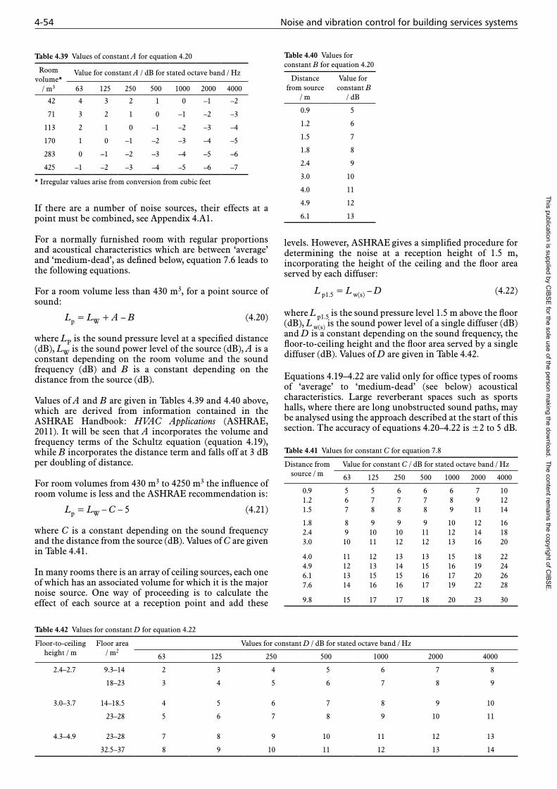
4-54 Noise and vibration control for building services systems
If there are a number of noise sources, their effects at a point must be combined, see Appendix 4.A1.
For a normally furnished room with regular proportions and acoustical characteristics which are between ‘average’ and ‘medium-dead’, as defined below, equation 7.6 leads to the following equations.
For a room volume less than 430 m3, for a point source of sound:
Lp = LW + A – B (4.20)
where LP is the sound pressure level at a specified distance (dB), LW is the sound power level of the source (dB), A is a constant depending on the room volume and the sound frequency (dB) and B is a constant depending on the distance from the source (dB).
Values of A and B are given in Tables 4.39 and 4.40 above, which are derived from information contained in the ASHRAE Handbook: HVAC Applications (ASHRAE, 2011). It will be seen that A incorporates the volume and frequency terms of the Schultz equation (equation 4.19), while B incorporates the distance term and falls off at 3 dB per doubling of distance.
For room volumes from 430 m3 to 4250 m3 the influence of room volume is less and the ASHRAE recommendation is:
Lp = LW – C – 5 (4.21)
where C is a constant depending on the sound frequency and the distance from the source (dB). Values of C are given in Table 4.41.
In many rooms there is an array of ceiling sources, each one of which has an associated volume for which it is the major noise source. One way of proceeding is to calculate the effect of each source at a reception point and add these
levels. However, ASHRAE gives a simplified procedure for determining the noise at a reception height of 1.5 m, incorporating the height of the ceiling and the floor area served by each diffuser:
L p1.5 = L w(s) – D (4.22)
where L p1.5 is the sound pressure level 1.5 m above the floor (dB), L w(s) is the sound power level of a single diffuser (dB) and D is a constant depending on the sound frequency, the floor-to-ceiling height and the floor area served by a single diffuser (dB). Values of D are given in Table 4.42.
Equations 4.19–4.22 are valid only for office types of rooms of ‘average’ to ‘medium-dead’ (see below) acoustical characteristics. Large reverberant spaces such as sports halls, where there are long unobstructed sound paths, may be analysed using the approach described at the start of this section. The accuracy of equations 4.20–4.22 is ±2 to 5 dB.
Table 4.39 Values of constant A for equation 4.20
Room volume*
/ m3
Value for constant A / dB for stated octave band / Hz
63 125 250 500 1000 2000 4000
42 4 3 2 1 0 –1 –2
71 3 2 1 0 –1 –2 –3
113 2 1 0 –1 –2 –3 –4
170 1 0 –1 –2 –3 –4 –5
283 0 –1 –2 –3 –4 –5 –6
425 –1 –2 –3 –4 –5 –6 –7
* Irregular values arise from conversion from cubic feet
Table 4.40 Values for constant B for equation 4.20
Distance from source
/ m
Value for constant B
/ dB
0.9 5
1.2 6
1.5 7
1.8 8
2.4 9
3.0 10
4.0 11
4.9 12
6.1 13
Table 4.42 Values for constant D for equation 4.22
Floor-to-ceiling height / m
Floor area / m2
Values for constant D / dB for stated octave band / Hz
63 125 250 500 1000 2000 4000
2.4–2.7 9.3–14 2 3 4 5 6 7 8
18–23 3 4 5 6 7 8 9
3.0–3.7 14–18.5 4 5 6 7 8 9 10
23–28 5 6 7 8 9 10 11
4.3–4.9 23–28 7 8 9 10 11 12 13
32.5–37 8 9 10 11 12 13 14
Table 4.41 Values for constant C for equation 7.8
Distance from source / m
Value for constant C / dB for stated octave band / Hz
63 125 250 500 1000 2000 4000
0.9 5 5 6 6 6 7 101.2 6 7 7 7 8 9 121.5 7 8 8 8 9 11 14
1.8 8 9 9 9 10 12 162.4 9 10 10 11 12 14 183.0 10 11 12 12 13 16 20
4.0 11 12 13 13 15 18 224.9 12 13 14 15 16 19 246.1 13 15 15 16 17 20 267.6 14 16 16 17 19 22 28
9.8 15 17 17 18 20 23 30
This publication is supplied by CIB
SE
for the sole use of the person making the dow
nload. The content remains the copyright of C
IBS
E.

Room sound levels 4-55
4.7.3 Source directivity
When the sound power of the duct termination has been calculated, a further step is required to assess whether the room influences the radiation from the termination. If the adjacent surfaces are acoustically non-absorbing, the influence depends on the location of the termination within the room, and affects only the direct sound. The reverberant sound is not changed by the location. A general consideration for sources is described below.
If the source is located in free space, a situation which could be approximated by a duct projecting into the centre of a room, the energy from the duct outlet spreads uniformly and, for the direct sound, the relevant relation for intensity is given by (see Appendix 4.A1):
I = P / 4 π r2 (4.23)
where I is the sound intensity (W·m–2), P is the sound power (W) and r is the distance from the source (m).
Figure 4.46 shows a further three basic locations for an outlet. If the termination is in the centre of a reflecting surface (position A), the sound propagates into half space due to reflections from the wall, so that, at any point, there is twice as much direct energy as before. This is an apparent doubling of the directly radiated source power, caused by reflections from one surface before the sound first reaches a listener. The result is a 3 dB increase in direct sound level.
If the termination is at one edge of the room (Figure 4.46, position B), where two reflecting surfaces meet, propagation is into a quarter space. There is an apparent quadrupling of the directly radiated sound caused by reflections from two
surfaces before the sound reaches a listener, leading to a 6 dB increase in the direct sound over the source located in free space.
If the termination is in a corner (Figure 4.46, position C), where three reflecting surfaces meet, propagation is into one-eighth space. This is an apparent eight-fold increase in the directly radiated source power, caused by reflections from three surfaces before the sound reaches a listener. This leads to a 9 dB increase in the direct sound over the source located in space.
These initial reflections from surfaces adjacent to the source do not affect the reverberant sound levels.
A general relation for effective sound power of the source is:
LW = (10 lg P) + (10 lg Q) + 120 (4.24)
where LW is the sound power level (dB), P is the sound power (W) and Q is a directivity factor. The directivity factor indicates how much more energy is received due to reflection of the sound by the adjacent surfaces. Under the conditions of reflective surfaces, as in Figure 4.46, Q takes values of 1 for a source in free space, and 2, 4 or 8 for positions A, B and C respectively.
If the adjacent surface is very absorbing, e.g. a suspended ceiling at higher frequencies, the sound will not be reflected from it and there will not be the simple theoretical inter-action described above. Use of these directivity concepts is approximate. (There are parallels with reflection of light from reflective or dull adjacent surfaces.)
Directivity is also an inherent property of some noise sources, which radiate preferentially in certain directions, irrespective of their location in a room. If a source is inherently highly directional, it will not be influenced by those adjacent surfaces which do not intercept its radiation. In general, when the dimensions of a source are large compared with the wavelength of the radiated sound, it becomes directional. For a grille or outlet in a room, Table 4.43 below can be used to determine the directivity correction factor (D2) for use in equation 4.18 above.
For situations outdoors, where sound is emitted from a duct opening to atmosphere or from a louvre located in a wall, the aperture directivity of the source can have a very significant effect on the direct sound pressure level received
A
BC
Figure 4.46 Outlet locations
Table 4.43 Corrections for directivity
Mounting position
Outlet area / m2
Corrections /dB for stated octave band centre frequency / Hz
125 250 500 1000 2000 4000 8000
A 0.01 +3 +4 +5 +6 +7 +8 +80.05 +4 +5 +6 +7 +8 +8 +90.1 +4 +6 +7 +8 +9 +9 +9
0.25 +5 +7 +7 +8 +9 +9 +91.0 +7 +8 +8 +9 +9 +9 +9
10.0 or more +9 +9 +9 +9 +9 +9 +9
B 0.01 +6 +6 +7 +7 +8 +8 +90.05 +7 +7 +8 +8 +9 +9 +90.1 +7 +8 +8 +9 +9 +9 +9
0.25 +8 +8 +8 +9 +9 +9 +91.0 +8 +9 +9 +9 +9 +9 +9
10.0 or more +9 +9 +9 +9 +9 +9 +9
C All areas +9 +9 +9 +9 +9 +9 +9
This publication is supplied by CIB
SE
for the sole use of the person making the dow
nload. The content remains the copyright of C
IBS
E.
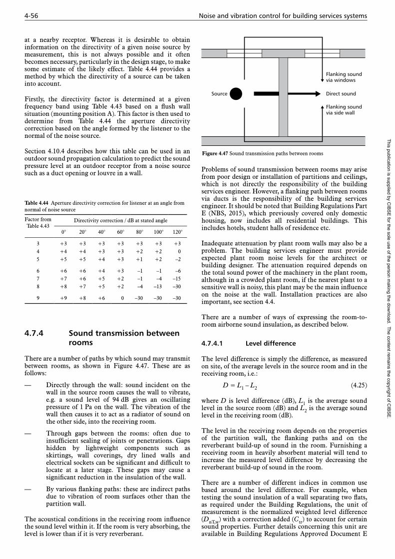
4-56 Noise and vibration control for building services systems
at a nearby receptor. Whereas it is desirable to obtain information on the directivity of a given noise source by measurement, this is not always possible and it often becomes necessary, particularly in the design stage, to make some estimate of the likely effect. Table 4.44 provides a method by which the directivity of a source can be taken into account.
Firstly, the directivity factor is determined at a given frequency band using Table 4.43 based on a flush wall situation (mounting position A). This factor is then used to determine from Table 4.44 the aperture directivity correction based on the angle formed by the listener to the normal of the noise source.
Section 4.10.4 describes how this table can be used in an outdoor sound propagation calculation to predict the sound pressure level at an outdoor receptor from a noise source such as a duct opening or louvre in a wall.
Table 4.44 Aperture directivity correction for listener at an angle from normal of noise source
Factor from Table 4.43
Directivity correction / dB at stated angle
0° 20° 40° 60° 80° 100° 120°
3 +3 +3 +3 +3 +3 +3 +34 +4 +4 +3 +3 +2 +2 05 +5 +5 +4 +3 +1 +2 –2
6 +6 +6 +4 +3 –1 –1 –67 +7 +6 +5 +2 –1 –4 –158 +8 +7 +5 +2 –4 –13 –30
9 +9 +8 +6 0 –30 –30 –30
4.7.4 Sound transmission between rooms
There are a number of paths by which sound may transmit between rooms, as shown in Figure 4.47. These are as follows:
— Directly through the wall: sound incident on the wall in the source room causes the wall to vibrate, e.g. a sound level of 94 dB gives an oscillating pressure of 1 Pa on the wall. The vibration of the wall then causes it to act as a radiator of sound on the other side, into the receiving room.
— Through gaps between the rooms: often due to insufficient sealing of joints or penetrations. Gaps hidden by lightweight components such as skirtings, wall coverings, dry lined walls and electrical sockets can be significant and difficult to locate at a later stage. These gaps may cause a significant reduction in the insulation of the wall.
— By various flanking paths: these are indirect paths due to vibration of room surfaces other than the partition wall.
The acoustical conditions in the receiving room influence the sound level within it. If the room is very absorbing, the level is lower than if it is very reverberant.
Flanking soundvia windows
Flanking soundvia side wall
Direct soundSource
Figure 4.47 Sound transmission paths between rooms
Problems of sound transmission between rooms may arise from poor design or installation of partitions and ceilings, which is not directly the responsibility of the building services engineer. However, a flanking path between rooms via ducts is the responsibility of the building services engineer. It should be noted that Building Regulations Part E (NBS, 2015), which previously covered only domestic housing, now includes all residential buildings. This includes hotels, student halls of residence etc.
Inadequate attenuation by plant room walls may also be a problem. The building services engineer must provide expected plant room noise levels for the architect or building designer. The attenuation required depends on the total sound power of the machinery in the plant room, although in a crowded plant room, if the nearest plant to a sensitive wall is noisy, this plant may be the main influence on the noise at the wall. Installation practices are also important, see section 4.4.
There are a number of ways of expressing the room-to-room airborne sound insulation, as described below.
4.7.4.1 Level difference
The level difference is simply the difference, as measured on site, of the average levels in the source room and in the receiving room, i.e.:
D = L1 – L2 (4.25)
where D is level difference (dB), L1 is the average sound level in the source room (dB) and L2 is the average sound level in the receiving room (dB).
The level in the receiving room depends on the properties of the partition wall, the flanking paths and on the reverberant build-up of sound in the room. Furnishing a receiving room in heavily absorbent material will tend to increase the measured level difference by decreasing the reverberant build-up of sound in the room.
There are a number of different indices in common use based around the level difference. For example, when testing the sound insulation of a wall separating two flats, as required under the Building Regulations, the unit of measurement is the normalized weighted level difference (DnT,w) with a correction added (Ctr) to account for certain sound properties. Further details concerning this unit are available in Building Regulations Approved Document E
This publication is supplied by CIB
SE
for the sole use of the person making the dow
nload. The content remains the copyright of C
IBS
E.

Room sound levels 4-57
(NBS, 2015) or International/British Standards (ISO 140-4 (ISO, 1998a), ISO 140-7 (ISO, 1998b), BS EN ISO 16283-1 (BSI, 2014a) and BS EN ISO 717 (BSI, 2013a/b)). Note that ISO 140-4 has been replaced by BS EN ISO 16283, but is still referred to in Building Regulations Approved Document E.
Of particular relevance to building services engineers is the unit used to describe the level difference provided by an air vent in an outside wall, such as a trickle vent or acoustic vent. The sound level difference quoted for the performance of a vent is Dn,e,w. This unit describes the level difference provided by a vent when inserted in a wall with an area of 10 m2 and then tested in a laboratory and adjusted or weighted to give a single figure rating. This method of measurement is used to indicate the sound reduction performance that can be achieved by placing the vent in a typical wall and allows comparisons to be made between the performance of different units.
4.7.4.2 Sound reduction index
The properties of the wall itself are given by the sound reduction index, R (sometimes referred to as the sound transmission loss) which is measured by standardised procedures in a test room (BS EN ISO 10140 (BSI, 2010a/b)). The reverberation time in the receiving room is standardised to To = 0.5 s, in order to allow for the effects in different rooms. A receiving room reverberation time, T, of 1 s will cause the level difference to be 3 dB higher than in a room having T = 0.5 s, i.e. 10 lg (T / 0.5) = 3 dB when T = 1 s.
The sound reduction index is a property of the separating wall material for samples measured in a laboratory according to current standards (BS EN ISO 10140-2 (BSI, 2010b) and this is the quantity which may be quoted in manu facturers’ literature. Some examples of sound reduction indices are given in Table 4.45, where the values are shown in decibels at octave band frequencies from 63 to 4000 Hz. Although most laboratory measurements have traditionally been made in third octave bands from 100 to 3150 Hz, as required in the older standards, measurement procedures now recommend extending the range from 50 Hz to 5000 Hz third octave bands. This recognises that the limited band of measurements from 100 Hz to 3150 Hz
do not provide sufficient information for a full assessment of subjective effects of noise.
Sound reduction index and level difference are related by the reverberation time, giving:
R = L1 – L2 + 10 lg (T) + 10 lg (S / 0.16 V) (4.26)
where R is the sound reduction index, L1 and L2 are the average sound levels in the source room and receiving room respectively (dB), T is the reverberation time (s), S is the total surface area of the room (m2) and V is the room volume (m3).
However, the validity of equation 4.26 reduces for short reverberation times.
4.7.4.3 Weighted sound reduction index
A single number representation of sound reduction is given by the weighted sound reduction index, Rw. This is obtained by comparing the measured attenuation–frequency curve with standardised curves, moderated by certain conditions. The value of the curve at 500 Hz then gives Rw (BS EN 717-1 (BSI, 2013a)).
There are differences between sound transmission under laboratory conditions and sound transmission in field conditions. The field measurement is often influenced by factors that are controlled in the laboratory, particularly flanking transmission and leakage through gaps. Table 4.45 gives typical values of sound reduction indices. Manufacturers’ data should be consulted for standard prefabricated office partitions.
4.7.5 Privacy and cross talk
Privacy describes the ability to talk within one space without being overheard in another space. In an open plan office, privacy is related to background noise and distance. Privacy between adjacent private offices depends on the amount of sound transmitted between the spaces and the background noise in the ‘listening’ room. The sound level received in a space should be below the criterion level for that space. Transmission is determined by the efficiency of
Table 4.45 Typical values of sound reduction index
Material Sound reduction index, R, for stated octave band / Hz
63* 125 250 500 1000 2000 4000
6 mm glass 15 18 23 30 35 27 32
Sealed double glazed window (6 mm outer, 12 mm air gap, 6 mm inner) 18 20 18 28 38 34 38
Separate window panes (5 mm outer, 150 mm air gap, 4 mm inner) 20 26 34 44 54 53 51
Acoustic double glazing (10 mm outer, 200 mm air gap, 6 mm inner) 26 37 46 45 47 57 64
Lightweight block (100 mm thick) e.g. ‘Thermalite’ 20 27 32 37 40 41 45
Galvanised steel sheet:
— 22 gauge (0.55 mm thick) 3 8 14 20 23 26 27— 16 gauge (1.6 mm thick) 9 14 21 27 32 37 43
200 mm reinforced concrete 36 42 41 50 57 60 65
Metal stud partition (2 × 12 5 mm plasterboard either side of 48 mm studs at 600 mm centres) 17 22 36 45 54 59 51
* Some of the values at 63 Hz are estimated
This publication is supplied by CIB
SE
for the sole use of the person making the dow
nload. The content remains the copyright of C
IBS
E.
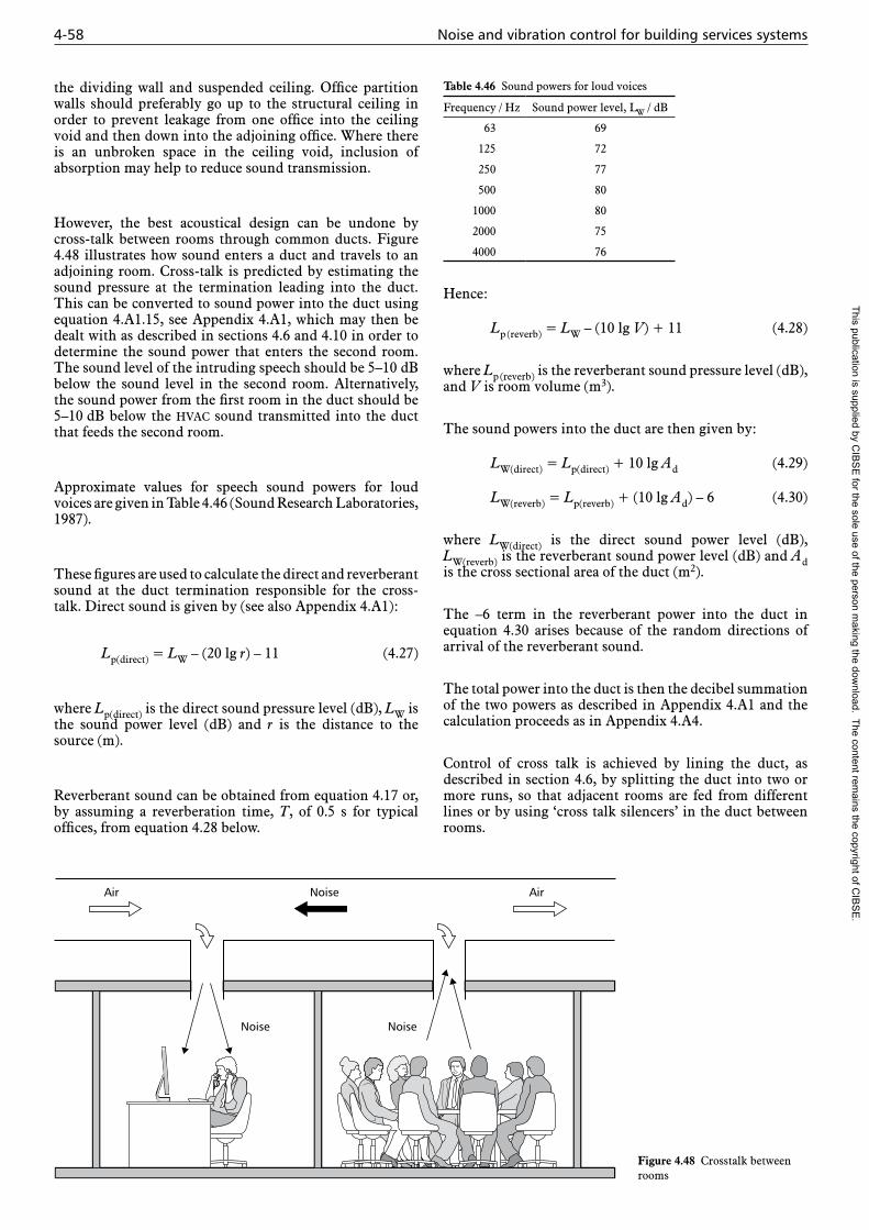
4-58 Noise and vibration control for building services systems
the dividing wall and suspended ceiling. Office partition walls should preferably go up to the structural ceiling in order to prevent leakage from one office into the ceiling void and then down into the adjoining office. Where there is an unbroken space in the ceiling void, inclusion of absorption may help to reduce sound transmission.
However, the best acoustical design can be undone by cross-talk between rooms through common ducts. Figure 4.48 illustrates how sound enters a duct and travels to an adjoining room. Cross-talk is predicted by estimating the sound pressure at the termination leading into the duct. This can be converted to sound power into the duct using equation 4.A1.15, see Appendix 4.A1, which may then be dealt with as described in sections 4.6 and 4.10 in order to determine the sound power that enters the second room. The sound level of the intruding speech should be 5–10 dB below the sound level in the second room. Alternatively, the sound power from the first room in the duct should be 5–10 dB below the hvac sound transmitted into the duct that feeds the second room.
Approximate values for speech sound powers for loud voices are given in Table 4.46 (Sound Research Laboratories, 1987).
These figures are used to calculate the direct and reverberant sound at the duct termination responsible for the cross-talk. Direct sound is given by (see also Appendix 4.A1):
Lp(direct) = LW – (20 lg r) – 11 (4.27)
where Lp(direct) is the direct sound pressure level (dB), LW is the sound power level (dB) and r is the distance to the source (m).
Reverberant sound can be obtained from equation 4.17 or, by assuming a reverberation time, T, of 0.5 s for typical offices, from equation 4.28 below.
Hence:
Lp (reverb) = LW – (10 lg V) + 11 (4.28)
where Lp (reverb) is the reverberant sound pressure level (dB), and V is room volume (m3).
The sound powers into the duct are then given by:
LW(direct) = Lp(direct) + 10 lg Ad (4.29)
LW(reverb) = Lp(reverb) + (10 lg Ad) – 6 (4.30)
where LW(direct) is the direct sound power level (dB), LW(reverb) is the reverberant sound power level (dB) and Ad is the cross sectional area of the duct (m2).
The –6 term in the reverberant power into the duct in equation 4.30 arises because of the random directions of arrival of the reverberant sound.
The total power into the duct is then the decibel summation of the two powers as described in Appendix 4.A1 and the calculation proceeds as in Appendix 4.A4.
Control of cross talk is achieved by lining the duct, as described in section 4.6, by splitting the duct into two or more runs, so that adjacent rooms are fed from different lines or by using ‘cross talk silencers’ in the duct between rooms.
Noise
Noise Noise
Air Air
Figure 4.48 Crosstalk between rooms
Table 4.46 Sound powers for loud voices
Frequency / Hz Sound power level, LW / dB
63 69
125 72
250 77
500 80
1000 80
2000 75
4000 76
This publication is supplied by CIB
SE
for the sole use of the person making the dow
nload. The content remains the copyright of C
IBS
E.

Transmission of noise to and from the outside 4-59
4.8 Transmission of noise to and from the outside
Transmission of noise into or out of buildings has important implications for the building services engineer, whether the noise is from building services within the building or because the building services themselves alter the sound insulation of a building, e.g. by creating a new aperture and thereby admitting external noise. Building services noise may also be transmitted to another area of the same building or to an adjacent building. Some building services equip-ment is located outside and its noise may affect the building it serves or neighbouring buildings. Reflection of noise from adjacent building surfaces should be taken into account, see section 4.7.3 and Noise control in building services
(Sound Research Laboratories, 1987).
4.8.1 Transmission of noise to the outside and to other rooms
Noise from building services travels to the outside in a number of ways. It might be created outside from a roof-mounted generator, chiller, air handling unit or condenser, or inside, such as from a fan or boiler plant. It then travels through louvres, ducts or the fabric of the building to the outside. It will be necessary to design the system to ensure that specified criteria are met outside the building. It is usual for the local authority to stipulate the criterion in such situations, to protect public open space or limit noise into nearby buildings.
Estimation of noise passing through the fabric of the building to the outside or to other parts of the building will generally require specialist knowledge of the sound insulation of materials. This is beyond the scope of this Guide, although general principles are given in section 4.7.4 and reference can also be made to BS EN 12354-4 (2000a). If the building services engineer concludes that estimation is required, this should be brought to the attention of the project manager.
Estimation of noise from externally located plant or duct openings and louvres is normally the responsibility of the building services engineer, although it is common to involve an acoustic specialist in this assessment. Section 4.10.4 sets out some principles concerning an assessment method.
4.8.2 Transmission of external noise to the inside
For the building services engineer, the transmission of noise from the outside into a room should be considered from two distinct aspects. The first is that considered in section 4.8.1 above, where noise from the plant, occurring or created outside a building, travels into the building through windows, the roof or any other element, including the services themselves. Generally, but not always, the building services engineer will have no control over the sound insulation of the building against external noise and it will be necessary to ensure that criteria are met solely by appropriate design of the plant. The second aspect is that of noise from other sources, such as road or rail traffic, aircraft or industrial noise, entering a building via its own services, an inlet or exhaust duct, trickle vent or perhaps an extract
fan. The opening for the fan or duct, or any gap around a duct, will have little insulation against noise from the outside and could seriously compromise the sound insulation of a building. Careful thought must be given to the sound insulation of the combined system.
Particular consideration should be given to how the building ventilation strategy might affect the transmission of noise into a building. For example, trickle ventilators will significantly reduce the sound insulation performance of a double glazed window. Acoustic ventilators (whose acoustic performance is rated in terms of Dn,e,w — refer to Annex E of BS EN ISO 10140-1 (BSI, 2010a) are common-place but they can affect the appearance of a building façade. Any strategy should therefore be developed with input from the architect and acoustician as well as the building services engineer.
Further guidance on the calculation of the transmission of external noise to the inside is given in BS EN ISO 12354-3 (BSI, 2000b) and also BS 8233 (BSI, 2014b).
4.8.3 Naturally ventilated buildings
Natural ventilation generally requires large apertures through the building envelope through which noise is easily transmitted. The low pressure drops required for natural ventilation limit the options available to attenuate the noise. Consequently, natural ventilation may be problematic for buildings on noisy sites.
The amount of noise transmitted through an aperture into a room is proportional to the size of the aperture and inversely proportional to the quantity of acoustic absorption in the room. The following formula applies:
L2 = L1 – R + 10 lg10 (S /A) (4.31)
where L2 is the internal noise level (dB), L1 is the external facade level (dB) (levels obtained by measurement on an open site, rather than immediately in front of a facade should have 3 dB added at all frequencies to obtain this value), R is the sound reduction index of the aperture (dB) (which can be assumed to be 0 dB in all relevant frequency bands for an aperture), S is the area of the aperture (m2) and A is the area of absorption (m2) in the room (normally approximately 10 m2 for a domestic room or cellular office).
As a general guide, a room with a partially open window will experience noise levels which are 10 to 15 dBA below the external noise level. A reasonable upper limit for noise in living rooms is 40 dBA (see BS 8233 (BSI, 2014b)) (expressed as the equivalent continuous level, Leq), so if the external noise level is more than 50–55 dBA Leq it may not be acceptable to rely on open windows for natural ventilation. Similarly, noise in a school classroom should not normally exceed 35 dBA Leq while meeting the minimum ven tilation requirements, so an open window may not be acceptable for school classrooms exposed to levels in excess of 45–50 dBA Leq.
On sites exposed to higher noise levels, it may be possible to use acoustic screening to reduce noise levels sufficiently to allow windows to be opened. For example if a close-boarded fence or earth bank is introduced next to a road or railway track, blocking the line of sight between it and a window, it is normally possible to reduce the external noise level by around 10 dBA. Comparable reductions can be
This publication is supplied by CIB
SE
for the sole use of the person making the dow
nload. The content remains the copyright of C
IBS
E.

4-60 Noise and vibration control for building services systems
obtained on the facades of buildings which face away from the noise source, or which benefit from incidental screening from other parts of the same building or development.
It may be possible to take advantage of this by ducting air from the quiet side of the building to rooms on the noisy side.
Where it is not feasible to affect the required noise reductions by site planning measures, it is necessary to consider what can be done in the design of the building. Attenuated ventilators are available which penetrate the building facade – either attenuated versions of window-mounted trickle ventilators, or units which are built into the external walls. Their overall acoustic performance is specified in terms of the weighted element normalised level difference (Dn,e,w) and the following formula applies:
L2 = L1 – Dn,e + 10 lg (Ao / A) (4.32)
where L2 is the internal noise level (dB), L1 is the external facade noise level (dB), Dn,e is the element normalised level difference (dB) of the ventilator (which varies with frequency), Ao is the reference absorption (10 m2) and A is the room absorption (normally approximately 10 m2 for a domestic room or cellular office).
Commercial wall-mounted units may be capable of achieving Dn,e,w values in the range 40–50 dB, but have limited equivalent open areas (typically 2500–4000 mm2). Where multiple units are required to achieve the necessary ventilation, the resulting noise level in the room will increase by 10 lg10 N, where N is the number of units.
Attenuated ventilators may also be used as part of a passive stack ventilation system, allowing air into rooms through the external walls. Air is discharged by the stack effect through ducts at roof level. If the external environmental noise level above the roof is high, then it may be necessary to incorporate in-line attenuators or sound absorbing linings into the discharge ductwork.
‘Windcatcher’ ventilators are capable of supplying and extracting air via a subdivided stack as a result of the action of the wind. This may obviate the need for wall-mounted attenuated ventilators. Where required, attenuation may be provided by introducing sound-absorbing linings in the airways.
A potential advantage of stack and ‘windcatcher’ ventilators is that on sites exposed to road or rail noise, the top of the stack will often be situated in a quieter location, reducing the need for noise control measures. This would not apply to aircraft noise.
The use of stack ventilation may give rise to sound insulation issues within the building. Where an air path must be provided between a room and a corridor, or atrium, it will be necessary to provide cross-talk attenuation which maintains the sound insulation performance of the corridor partition. This might take the form of an attenuated ventilator, a cross-talk attenuator, or an acoustically-lined builders’ work duct.
Where multiple rooms are served by the same ventilation stacks, it may be necessary to install cross-talk attenuators in the stacks to preserve the sound insulation between the linked rooms.
4.9 Criteria for noise from building services systems
Please note that a more comprehensive discussion on noise criteria is contained in CIBSE Guide A, section 1.10, which also includes guidance on selection of appropriate criteria for different applications.
4.9.1 Objective
Noise criteria are used for various purposes including:
— setting performance standards for a space or building
— providing guidance for the detailed acoustic design of a space or building
— acting as benchmarks in the investigation of noise problems or complaints.
Some factors influencing noise levels may be outside the control of the building services design engineer or may be unknown at an early enough stage — for example, the acoustic properties of construction materials and finishes — and the engineer may have to make assumptions about typical spaces, as described in section 4.7 of this Guide.
The designer with responsibility for building services noise must make sure it complies with the agreed criteria at specified locations. In addition to building services noise, a building may be affected by noise related to its occupation related activity, e.g. office machines, telephones, conver-sation, televisions. Compliance with noise criteria for building services is normally considered in the absence of activity noise.
Noise from sources not directly produced by building services but affected by the design must also be considered. For example, noise transmission between spaces via building services ductwork which effectively reduces the sound insulation between those spaces. Naturally ventilated buildings must be designed to control the transmission of noise through ventilation paths even though the noise sources may be external to the building and not under the control of the designer.
In developing selection criteria, the needs of the occupants have to be balanced against the costs of noise control. In a workplace, these needs may include health, comfort, concentration and absence of errors for individuals, and communication with others either directly or by telephone. In a residential building, these needs include comfort and the ability to sleep properly.
4.9.2 Choosing noise criteria parameters
4.9.2.1 Overall noise levels
To facilitate communication about noise levels (e.g. between client and designer) it is necessary to have a simple way of quantifying overall noise levels from building services and a single figure parameter is usually used for this purpose (e.g. dBA, NR, Nc and others).
This publication is supplied by CIB
SE
for the sole use of the person making the dow
nload. The content remains the copyright of C
IBS
E.

Criteria for noise from building services systems 4-61
In the UK, the dBA and NR level are in the most widespread use. For environmental noise from building services and all forms of transportation, and for internal noise from environmental sources, the dBA is used. However, while the dBA is used in most UK standards and guidance for internal building services noise, the NR is still widely used in the building services industry. This may lead to dangers for the designer: the internal noise levels from traffic may meet the dBA criterion and the internal noise from building services may meet the NR criterion, but the total noise level from both may fail to meet the BREEAM total noise level which is usually specified in dBA. The only way for the designer to be sure of meeting a BREEAM dBA criterion is to specify internal building services noise levels in dBA — if necessary, in addition to an NR level. It should be noted that, unlike the NR, Nc, Rc etc, the dBA level from one source can be added (logarithmically) to that of another to get the total dBA level.
In the USA, the Nc level is most widely used instead of the NR level, although the dBA now sits alongside it in the most recent ASHRAE guidance.
Criteria
Further descriptions of various single noise parameters are given in CIBSE Guide A, section 1.10, where Table 1.22 gives NR criteria for various occupied spaces.
4.9.2.2 Noise quality
No single figure noise level parameter can represent the spectral characteristics of a noise and different noises with the same overall noise level may sound completely different and have different acceptability – e.g. one may be an unacceptable rumbling noise and another an acceptable characterless noise.
In the UK, this problem has been addressed only in a simple way for specification and commissioning criteria: a noise with disturbing characteristics is penalized by 5 dB. However, this implies that a noise with annoying character-istics may become acceptable by making it quieter and there is little to support this idea. Some countries have dealt with low frequency noise (rumble) by imposing a specific low frequency noise level limit. In the USA, spectral acceptability has been addressed most recently by cal-culating a quality index (qi), used in conjunction with an overall level (Rc). The Rc/qi system was developed as a troubleshooting tool but was for some time recommended for performance criteria in the ASHRAE Fundamentals Handbook. However, it proved too unwieldy for everyday use and the current edition of the Handbook (ASHRAE, 2013) gives noise level criteria using dBA and Nc parameters with dBC used to provide a simple limit for low frequency noise.
4.9.2.3 Time variation
Noise levels usually vary with time and this is taken into account by the use of statistical descriptors such as the Leq (a widely used logarithmic average), Lmax, and Ln. When applied to noise measured in dBA, these are designated LAeq, LAmax, LAn, and so on.
The Leq over a period of 1–5 minutes is commonly used when measuring building services noise levels in the UK
and it is this value that is compared with the specified dBA or NR level.
Measurement of building services noise in the presence of significant traffic noise is often done using the L90 measure, i.e. noise levels exceeded for 90% of the time. This is an attempt to assess the noise level during traffic noise lulls.
As a general rule, any fluctuation in overall building services noise levels which is subjectively noticeable may well be judged unacceptable.
4.9.3 Design criteria
In addition to meeting building performance criteria, which are usually specified in terms of single figure parameters (dBA, NR), the designer should consider the spectral characteristics to ensure that the noise is reasonably spectrally balanced. Designing just to meet an overall dBA level or an NR or Nc curve at each frequency is not sufficient.
It is useful to have a target spectrum for the design process and, in the UK, it is common practice to design to meet an NR curve even though it is known that this does not represent a pleasant spectrum. A better alternative might be to design to a target spectrum which falls with frequency at around 5 dB/octave to provide a more balanced sound.
The relationship between NR and dBA values depends upon the spectral characteristics of the noise. However, for ordinary intrusive noise found in buildings, dBA is usually between 4 and 8 dB greater than the corresponding NR, and a conversion of 5–6 dB is often used. If in doubt, both should be determined for the specific noise octave band spectrum under consideration.
4.9.4 Using dBA, dBC, NR and NC levels
4.9.4.1 dBA and dBC
The dBA level of a noise may be measured directly with all sound levels meters and the dBC with most meters.
The A and C frequency weightings are defined in BS EN 61672-1: Electroacoustics. Sound level meters. Specifications (BSI, 2013c).
The dBA and dBC noise levels may also be calculated from predicted octave or ⅓-octave bands by applying the appropriate frequency weightings to the 1/1- or 1/3-octave band sound pressure levels and then logarithmically combining the weighted levels.
The total of two or more A- or C-weighted noise levels may also be calculated by the logarithmic combination method.
See Appendix 4.A1 for information about combining decibel values and calculating A-weighted values.
4.9.4.2 NR levels
NR levels cannot be measured directly on most sound level meters but must be calculated from the measured octave band levels.
This publication is supplied by CIB
SE
for the sole use of the person making the dow
nload. The content remains the copyright of C
IBS
E.
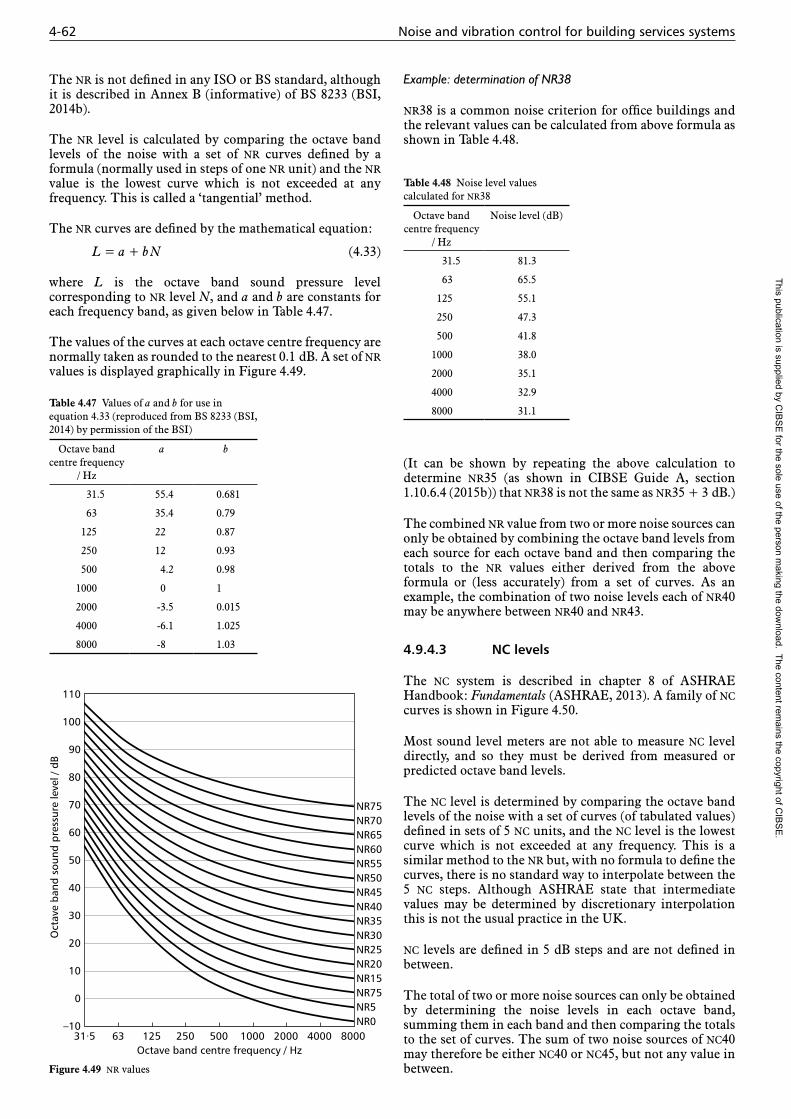
4-62 Noise and vibration control for building services systems
The NR is not defined in any ISO or BS standard, although it is described in Annex B (informative) of BS 8233 (BSI, 2014b).
The NR level is calculated by comparing the octave band levels of the noise with a set of NR curves defined by a formula (normally used in steps of one NR unit) and the NR value is the lowest curve which is not exceeded at any frequency. This is called a ‘tangential’ method.
The NR curves are defined by the mathematical equation:
L = a + b N (4.33)
where L is the octave band sound pressure level corresponding to NR level N, and a and b are constants for each frequency band, as given below in Table 4.47.
The values of the curves at each octave centre frequency are normally taken as rounded to the nearest 0.1 dB. A set of NR values is displayed graphically in Figure 4.49.
Example: determination of NR38
NR38 is a common noise criterion for office buildings and the relevant values can be calculated from above formula as shown in Table 4.48.
(It can be shown by repeating the above calculation to determine NR35 (as shown in CIBSE Guide A, section 1.10.6.4 (2015b)) that NR38 is not the same as NR35 + 3 dB.)
The combined NR value from two or more noise sources can only be obtained by combining the octave band levels from each source for each octave band and then comparing the totals to the NR values either derived from the above formula or (less accurately) from a set of curves. As an example, the combination of two noise levels each of NR40 may be anywhere between NR40 and NR43.
4.9.4.3 NC levels
The Nc system is described in chapter 8 of ASHRAE Handbook: Fundamentals (ASHRAE, 2013). A family of Nc curves is shown in Figure 4.50.
Most sound level meters are not able to measure Nc level directly, and so they must be derived from measured or predicted octave band levels.
The Nc level is determined by comparing the octave band levels of the noise with a set of curves (of tabulated values) defined in sets of 5 Nc units, and the Nc level is the lowest curve which is not exceeded at any frequency. This is a similar method to the NR but, with no formula to define the curves, there is no standard way to interpolate between the 5 Nc steps. Although ASHRAE state that intermediate values may be determined by discretionary interpolation this is not the usual practice in the UK.
Nc levels are defined in 5 dB steps and are not defined in between.
The total of two or more noise sources can only be obtained by determining the noise levels in each octave band, summing them in each band and then comparing the totals to the set of curves. The sum of two noise sources of Nc40 may therefore be either Nc40 or Nc45, but not any value in between.
Table 4.47 Values of a and b for use in equation 4.33 (reproduced from BS 8233 (BSI, 2014) by permission of the BSI)
Octave band centre frequency
/ Hz
a b
31.5 55.4 0.681
63 35.4 0.79
125 22 0.87
250 12 0.93
500 4.2 0.98
1000 0 1
2000 -3.5 0.015
4000 -6.1 1.025
8000 -8 1.03
110
100
90
80
70
60
50
40
30
20
10
0
–10
Oct
ave
band
sou
nd p
ress
ure
leve
l / d
B
Octave band centre frequency / Hz6331·5
NR75NR70NR65NR60NR55NR50NR45NR40NR35NR30NR25NR20NR15NR75NR5NR0
250125 500 1000 2000 80004000
Figure 4.49 NR values
Table 4.48 Noise level values calculated for NR38
Octave band centre frequency
/ Hz
Noise level (dB)
31.5 81.3
63 65.5
125 55.1
250 47.3
500 41.8
1000 38.0
2000 35.1
4000 32.9
8000 31.1
This publication is supplied by CIB
SE
for the sole use of the person making the dow
nload. The content remains the copyright of C
IBS
E.

Noise prediction of sound pressure levels from building services 4-63
4.10 Noise prediction of sound pressure levels from building services
This section uses some of the key principles introduced in sections 4.6, 4.7, 4.8 and demonstrates, by way of worked examples, how predictions of noise transmission within duct systems can be made to determine sound pressure levels both within rooms and also at external receptors.
The calculation of noise emissions from a duct system involves the consideration of at least two and sometimes all four of the following:
— room effect: in the worst affected receiving room
— system noise: produced at the duct air entry/exit points
— breakout/break-in noise: produced at any point along the duct system
— noise propagation to outside: as measured at a receptor point.
Each of these elements assists in establishing the extent to which the noise produced by a fan or duct component, such as a volume control damper, must be attenuated to ensure the required noise design criterion in a given room is not exceeded.
The prediction of each of the above is discussed in turn below, but this section begins by considering the two most commonly encountered elements, room effect and system noise.
This section sets out in tabular form example procedures for calculating the sound pressure level in a room due to noise from a ventilation system.
The procedure involves two basic stages:
(1) Calculation of the maximum permissible sound power level at a grille to avoid exceeding the room noise design criterion, based on either the diffuse field method or the Schultz method.
(2) Calculation of the actual sound power level at the grille, taking account of the noise attenuating and generating properties of each duct system component, including attenuation of duct elements, noise generation due to airflow across duct elements, and noise break-out from and break-in to duct elements.
In the prediction process, each component of the hvac system is considered separately. Components of interest might be the fan, duct, branch, elbow (or bend), etc., finally leading to the duct termination at the room.
Figure 4.51 below is used to illustrate the prediction procedures, where it is required to predict the noise in the room at a distance of 1.5 m from the nearest grille or grilles.
4.10.1 Room effect
Table 4.49 below sets out the calculation of the maximum permissible sound pressure level in a room based on ensuring the noise design criterion of NR35 is not exceeded in the office space. The procedure demonstrates the diffuse field method which is commonly used in the UK but is most appropriate for a room with reverberant conditions or ‘live’ acoustic conditions. For rooms with average or ‘dead’ acoustic conditions, a more conservative result is likely to result.
Step 1:
— Select the worst affected room(s).
— This is often obvious from an inspection of the duct layout drawings, being the room with the grille located closest to the fan and/or the nearest room with the most stringent noise criterion, i.e. the most noise sensitive room. It is important however to be aware that air noise regeneration from a grille could affect more distant rooms so should be considered when assessing a duct system by checking duct velocities are sufficiently low (see Table 4.15).
— Where there is a risk of noise breakout, further calculations may be required. Figure 4.52 demonstrates how a duct passes through a conference room before reaching an office where the first grilles are located. A calculation for both rooms would be required here to establish which dictates the system noise reduction (duct attenuator) requirements.
Step 2:
— Confirm the required noise room criterion, for example NR35 (see section 4.9 and CIBSE Guide A (2015b), section 1.10, Table 1.22)
80
70
60
50
40
30
20
10
0
Oct
ave
band
sou
nd p
ress
ure
leve
l / d
B
Octave band centre frequency / Hz63
NC65
NC60
NC55
NC50
NC45
NC40
NC35
NC30
NC25
NC20
NC15
250125 500 1000 2000 80004000
Figure 4.50 Nc values
This publication is supplied by CIB
SE
for the sole use of the person making the dow
nload. The content remains the copyright of C
IBS
E.

4-64 Noise and vibration control for building services systems
Step 3:
— Using procedures described in section 4.7.1 and shown in Tables 4.49 and 4.50 below, establish the maximum permissible sound power level at the grille or grilles closest to the listener. Alternatively, determine the maximum permissible breakout sound power level, see section 4.6.10.
— The calculation in Table 4.49 determines the maximum permissible sound power level at a grille to avoid exceeding NR35 within the example office space shown in Figure 4.51 using the diffuse field method.
— To achieve the same result using the Schultz method, the prediction procedure set out in Table 4.50 can be adopted. This gives a similar but slightly less conservative result and has been developed from empirical measurements in rooms with average acoustic conditions (see section 4.7 of this Guide).
Having established how much sound power is permissible at the grille of the room, it is now necessary to assess the actual sound power that will occur as a result of the fan and duct system serving the room, as outlined in section 4.10.2 below.
Schedule of grilles
System SizeRef
Supply 350 × 350 0·2 m3/sS1
Supply 350 × 350 0·2 m3/sS2
Extract 450 × 450 0·4 m3/sE1
Volume
5 m
400 × 400
2·4 m3/s at 240 Pa 600 × 400
Fan F1
Vane axialdiam. = 0·6 mPeak eff. = 85%Actual eff. = 75%
Roomheight2·6 m
250 × 300 int.(25 mm lining)
300 × 300 ext.
OFFICE ROOM
CONFERENCEROOM
3 m
8 m
S1
S2
E1
1·5 m
Distance toreceiver
1·5 m
1·5 m
3·0 m
Figure 4.51 Example ventilation system
Table 4.49 Example calculation of room effect for the office space shown in Figure 4.51 using diffuse field method
Sound component Reference or calculation Value at stated octave band centre frequency / Hz
125 250 500 1000 2000 4000
NR35 Sound pressure levels NR curves (CIBSE Guide A, section 1.10)
52 45 39 35 32 30
Reverberant room effectNo. of sources (N = 3) –10 lg N –5 –5 –5 –5 –5 –5Room surface area correction –10 lg (4 / S) 16 16 16 16 16 16Acoustic conditions correction (average) 10 lg (–a / (1 – –a)), Table 4.37 –11 –9 –7 –5 –4 –3
Permissible reverb swl at grille (1) 52 47 43 41 39 38
Direct room effectNo. of sources (N = 2) –10 lg N –3 –3 –3 –3 –3 –3
Distance to listener (r = 1.5 m) (20 lg r) + 11 +15 +15 +15 +15 +15 +15Directivity correction (outlet area = 0.12 m2, mounting position A)
Table 4.43 –4 –6 –7 –8 –9 –9
Permissible direct swl at grille (2) 60 51 44 39 35 33
Logarithmically combining (1) and (2) (see Appendix 4.A1):
Total permissible swl at grille 51 46 40 37 34 32
This publication is supplied by CIB
SE
for the sole use of the person making the dow
nload. The content remains the copyright of C
IBS
E.
Noise prediction of sound pressure levels from building services 4-65
4.10.2 System noise
The duct system noise is determined by establishing the noise produced by a given duct component, such as a fan, or by airflow across a damper, and offsetting this by the attenuation provided by each duct component in turn. The calculation can be relatively simple where only the attenuation of each duct component is offset against the noise produced by a fan. It increases in complexity where airflow generated noise at each duct component is also taken into account. Procedures for calculating the airflow noise generated at a duct component are given in Appendix 4.A2. The prediction of airflow generated noise however is commonly avoided, except in the most noise critical situations (in auditoria, music studios and theatres for example) by selecting appropriate design airflows, see section 4.5.2.
The duct system calculation is commonly undertaken from the noise source, i.e. from the fan, towards the grille. There are however advantages in working from the grille to the fan, particularly when it is necessary to include a consideration of airflow generated noise. This allows a check to be made of the noise resulting at the grille as a result of airflow noise alone, by accounting for the downstream system attenuation and summation of airflow noise at all intervening fittings. This approach, if undertaken for each duct fitting, will identify if and when the permissible sound power levels at a grille are exceeded as a result of airflow at a given fitting. If so, duct velocities can be reduced (see Table 4.18) or alternatively an attenuator inserted downstream of the given duct fitting. On reaching the fan, the fan noise is then introduced into the system and the sound power at each duct fitting adjusted accordingly.
A description of the simple calculation procedure is given below with information on the more complex procedures given in parentheses where appropriate:
(1) Determine the attenuation provided by each duct component in turn. (Determine the air noise generation characteristics of each duct component in turn.)
(2) Working ideally from the grille to the fan, sum the overall attenuation provided by the duct system. (Determine the successive effects of system components on the noise as it propagates in the duct, adding the effects, which may be negative (noise attenuation) or positive (noise regeneration)). Data on component effects should be provided by manufacturers or estimated using data in section 4.6 and Appendix 4.A2.
(3) Determine the noise power of the source (fan) from manufacturers’ data or, for initial design purposes, using empirical fan laws (section 4.3.2).
(4) Calculate the actual sound power level at the grille. A sample calculation of this procedure is given in Table 4.51.
(5) Calculate the attenuator requirements by subtracting the result of Step 3 in 4.10.1 above from the result of Step 4 above.
These steps are to be carried out at all frequencies required for the criterion used. A worked example demonstrating the above procedures for the duct system shown in Figure 4.51 is given below in Table 4.51. For the sake of simplicity, airflow noise is excluded from this worked example.
Table 4.50 Example calculation of room effect for the office space shown in Figure 4.51 using the Schultz method
— Number of sources = 3 (i.e. 1.5 m, 1.5 m, 3 m)
— Room volume = 8 m× 5 m × 2.6 m = 104 m3
— Rearranging equation 4.19: LW = Lp + 10 lg r + 5 lg V + 3 lg f – 12
Sound component Reference or calculation Value at stated octave band centre frequency / Hz
125 250 500 1000 2000 4000
NR35 Sound pressure levels NR curves (CIBSE Guide A, section 1.10)
52 45 39 35 32 30
Source 1Distance correction (r = 1.5 m) 10 lg r +2 +2 +2 +2 +2 +2Room volume correction (V = 104 m3) 5 lg V +10 +10 +10 +10 +10 +10Frequency correction 3 lg f +6 +7 +8 +9 +10 +11Constant –12 –12 –12 –12 –12 –12 –12
Permissible swl at grille due to source 1 58 52 47 44 42 41
Source 2Distance correction (r = 1.5 m) 10 lg r +2 +2 +2 +2 +2 +2Room volume correction (V = 104 m3) 5 lg V +10 +10 +10 +10 +10 +10Frequency correction 3 lg f +6 +7 +8 +9 +10 +11Constant –12 –12 –12 –12 –12 –12 –12
Permissible swl at grille due to source 2 58 52 47 44 42 41
Source 3Distance correction (r = 3 m) 10 lg r +5 +5 +5 +5 +5 +5Room volume correction (V = 104 m3) 5 lg V +10 +10 +10 +10 +10 +10Frequency correction 3 lg f +6 +7 +8 +9 +10 +11Constant –12 –12 –12 –12 –12 –12 –12
Permissible swl at grille due to source 3 61 55 50 47 45 44
Combining results for sources 1, 2 and 3 logarithmically:
Total permissible swl at one grille 54 48 43 40 38 37
This publication is supplied by CIB
SE
for the sole use of the person making the dow
nload. The content remains the copyright of C
IBS
E.

4-66 Noise and vibration control for building services systems
A commercial silencer is then selected so that the attenuation at each frequency band is achieved. This is normally dictated by the attenuation requirements at the low frequency octave bands such as 125 Hz and 250 Hz (8 dB and 10 dB respectively in the above example). Note that in more detailed calculations, it is common to include the 63 Hz and 8000 Hz octave band calculations as well. These are omitted here for simplicity.
The choice of a commercial silencer needs to take account of not only the attenuation requirements as calculated above but also the pressure drop allowable through the silencer and also its self noise generation characteristics, caused by the flow of air through its splitter elements. The physical size of the silencer must also be considered to ensure it will fit within the duct system design parameters.
Once a provisional silencer selection has been made, it is necessary to check that the additional room noise design criteria are satisfied, including the dBA and dBC values, plus any other indices that may be relevant to the room in question. Appendix 4.A1 sets out how to calculate the dBA and dBC parameters from the room sound pressure levels.
The example above allows the selection of a silencer to protect the acoustic conditions within the office space shown in Figure 4.51. However, this silencer will not necessarily protect the acoustic conditions within the conference room shown in Figure 4.51. This is because noise breakout through the duct that passes through the conference room may exceed the more stringent noise criterion of NR25 in this more critical space. A noise breakout calculation needs to be undertaken to assess any additional silencer attenuation requirements, as detailed in section 4.6.10.
4.10.2.1 Multiple sources
A room will normally have more than one noise source from the hvac systems, e.g. multiple duct outlets, break-out from a box or a duct in the ceiling void etc. It is the
summation of the noise from these sources which must meet the criterion, where summation is carried out as in Appendix 4.A1. Consequently, where there are multiple sources, the noise from each must be lower than the criterion and, for example, the silencer attenuation derived above, may need to be increased. Return air ducts must be included.
4.10.2.2 Computer predictions
Many organisations have building services noise prediction software, either developed in-house or obtained from an outside supplier. Refer to Appendix 4.A7 for further information.
4.10.3 Breakout/break-in noise
The calculation of the breakout of sound from a duct (as it passes through a plant room for example) is described in section 4.6.10. The principles of this are described below along with the general principles of how to calculate the break-in of sound to a duct:
Breakout
(1) Determine the sound power level in the duct at the point of duct entry to the room closest to the fan.
(2) Subtract the attenuation provided by the duct system in the room (which is normally negligible unless the duct is lined or lagged).
(3) Calculate the duct surface area within the room or the length of duct, to determine the length effect, see section 4.6.10.
(4) Establish the transmission loss out of the duct wall.
(5) Determine the sound power level breaking out of the duct using equation 4.11 in section 4.6.10.
Table 4.51 Example calculation of duct system attenuation requirements / dB
Sound component Reference or calculation
Value at stated octave band centre frequency (Hz)
125 250 500 1000 2000 4000
10 Fan swl delivered to system Section 4.3.2 82 80 80 80 78 75
9 Duct (4 L × 0.6 W × 0.4 H) (mean diam. = 0.5 m) Table 4.19 –2 –1 0 0 0 0
8 Volume control damper 0 0 0 0 0 0
7 Duct (6 L × 0.6 W × 0.4 H) (mean diam. = 0.5 m) Table 4.19 –2 –2 –1 –1 –1 –1
6 Mitre bend (with TV) (0.6 W) Table 4.23 –1 –4 –6 –4 –4 –4
5 Duct (3 L × 0.6 W × 0.4 H) (mean diam. = 0.5 m) Table 4.19 –1 –1 0 0 0 0
4 Junction area ratio = AB1 / (AB1 + AB2) = 0.319 Figure 4.34 –5 –5 –5 –5 –5 –5
4a Bend effect* (0.25 W) Table 4.22 0 –1 –5 –8 –4 –3
3 Lined duct (1.5 L × 0.25 W × 0.34 H) (pd / Ad = 13.3) Table 4.20(a) –1 –3 –8 –19 –18 –12
2 Mitre bend (without TV) (0.3 W) Table 4.22 0 –1 –5 –8 –4 –3
1 Grille (0.25 W × 0.35 H) (d = √ (4 A / π) = 0.33 m) Table 4.25 –8 –4 –1 0 0 0
Total attenuation in system 20 22 31 45 36 28
Actual swl at grille 62 58 49 35 42 47
Permissible swl at grille (from Schultz’s room effect calculation) 54 48 43 40 38 47
Silencing required 8 10 6 0 4 10
* Where a junction involves a 90° or greater turn-off from the main branch duct, it may be appropriate to include an additional bend attenuation allowance.
This publication is supplied by CIB
SE
for the sole use of the person making the dow
nload. The content remains the copyright of C
IBS
E.
Noise prediction of sound pressure levels from building services 4-67
(6) Calculate the resultant sound pressure level in the room using the equations in section 4.7.2 and accounting for the fact that the duct forms a line source as explained in section 4.6.10.
(7) Compare this with the room noise design criterion and, if greater, determine the additional duct attenuation requirements.
(8) Select an attenuator for placement upstream (between fan and receiving room) that satisfies all attenuation requirements).
Break-in
(1) Determine the reverberant sound pressure level incident on the duct surface.
(2) Calculate the duct surface area within the room.
(3) Establish the transmission loss in of the duct wall. This is usually less than the transmission loss referred to in section 4.6.10 and can be determined by a method described by Ver (1984).
(4) Calculate the sound power level leaving the duct at the point of exit from the room.
(5) Undertake a system noise calculation as described in section 4.10.2 for the worst affected room downstream of this point of noise break-in.
4.10.4 Noise propagation to outdoors
There are a variety of conditions that can arise on a project requiring the prediction of noise transmission to outdoors, including:
— Roof mounted plant such as generators, chillers, air handling units, extract fans, dry air coolers and condensers.
— Air inlet or extract duct terminations at roof level or in a façade.
— Noise breakout from a duct on a roof or situated on an external wall.
— Louvred openings or ventilation grilles, either ducted or non-ducted.
— External plant at ground level or an intermediate level, such as chillers and condensers.
The prediction of noise propagation to a nearby receptor follows a similar procedure for each of the above although the specific methodology will depend on the individual circumstances. A detailed methodology is provided in BS EN 12354-4 (BSI, 2000a). The procedures relate primarily to noise emissions from buildings and building facades, such as plant rooms, rather than from building services systems. Some guidance is however given for louvred openings.
For the situations described in the bullet points above, the general principles relate to the following equation:
Lp,out = LW + D1 + D2 (4.34)
where Lp,out is the free field sound pressure level at the receptor point (for a façade sound pressure level, such as 1 metre from a window, an addition of 2–3 dB is required), LW is the sound power level of the plant item or at the duct entry/exit or louvre, D1 is the sound reduction resulting from geometrical spreading and D2 is a correction to account for the directivity of the source and/or its proximity to reflective surfaces.
A description of the general principles above is as follows:
(1) Establish the sound power level of the plant item or at the entry/exit point of the louvre or duct. Use the methodology described in section 4.10.2 for this purpose.
(2) Determine the distance from the noise source to the receiver and calculate the noise reduction resulting from the geometric spreading of sound, see Appendix 4.A1.
(3) Establish or estimate the directivity characteristics of the noise source, taking account of any reflective surfaces in the vicinity as necessary, see section 4.7.3.
(4) Calculate the resultant sound pressure level at the nearest noise sensitive receptor, allowing for any façade reflection effects as necessary by the addition of 2–3 dB. This is required when a criterion is set at a distance of 1 m from a façade for example.
(5) Establish the design criterion at the receptor and, by comparison with the calculated resultant sound pressure level, determine any attenuation requirements.
(6) Select an appropriate noise mitigation measure, such as an attenuator (for ducted systems), an acoustic louvre (for vented systems), and/or a suitable screen, barrier or enclosure for roof mounted or outdoor plant items. Consider alternative mitigation measures as appropriate.
This section sets out, in descriptive and tabular form, example procedures for calculating the sound pressure level at an external receptor due to noise from a louvred ventilation opening in an external wall. The procedure involves the following basic steps:
(1) Establish the sound power level (LW) at the entry/exit point of the acoustic louvred opening. This can be done using the methods described in 4.10.2.
(2) Calculate the correction factor (D1) to account for the attenuation arising from the geometric spreading of noise from the louvre to the external receptor. Appendix 4.A1.7 contains the basic equation for this assuming radiation into free space. The relevant expression for the correction factor in this case is [(–20 lg r) – 11].
(3) Obtain or calculate a directivity correction factor (D2) to account for the source directivity characteristics and also any reflective surfaces near the source. This process may involve the application of two separate corrections, one to account for the directivity of the sound source (in this case the
This publication is supplied by CIB
SE
for the sole use of the person making the dow
nload. The content remains the copyright of C
IBS
E.
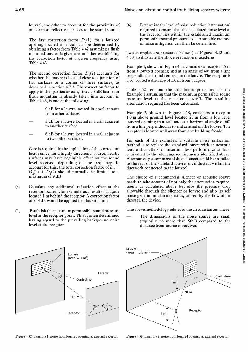
4-68 Noise and vibration control for building services systems
louvre), the other to account for the proximity of one or more reflective surfaces to the sound source.
The first correction factor, D2(1), for a louvred opening located in a wall can be determined by obtaining a factor from Table 4.42 assuming a flush mounted louvre of a given area and then establishing the correction factor at a given frequency using Table 4.43.
The second correction factor, D2(2) accounts for whether the louvre is located close to a junction of two surfaces or a corner of three surfaces, as described in section 4.7.3. The correction factor to apply in this particular case, since a 3 dB factor for flush mounting is already taken into account in Table 4.43, is one of the following:
— 0 dB for a louvre located in a wall remote from other surfaces
— 3 dB for a louvre located in a wall adjacent to another surface
— 6 dB for a louvre located in a wall adjacent to two other surfaces.
Care is required in the application of this correction factor since, for a highly directional source, nearby surfaces may have negligible effect on the sound level received, depending on the frequency. To account for this, the total correction factor of D2 = D2(1) + D2(2) should normally be limited to a maximum of 9 dB.
(4) Calculate any additional reflection effect at the receptor location, for example, as a result of a façade located 1 m behind the receptor. A correction factor of 2–3 dB would be applied for this situation.
(5) Establish the maximum permissible sound pressure level at the receptor point. This is often determined having regard to the prevailing background noise level at the receptor.
(6) Determine the level of noise reduction (attenuation) required to ensure that the calculated noise level at the receptor lies within the established maximum permissible sound pressure level. A suitable method of noise mitigation can then be determined.
Two examples are presented below (see Figures 4.52 and 4.53) to illustrate the above prediction procedures.
Example 1, shown in Figure 4.52 considers a receptor 15 m from a louvred opening and at an angle of 40° from a line perpendicular to and centred on the louvre. The receptor is also located a distance of 1.0 m from a façade.
Table 4.52 sets out the calculation procedure for the Example 1 assuming that the maximum permissible sound pressure level at the receptor is NR45. The resulting attenuation required has been calculated.
Example 2, shown in Figure 4.53, considers a receptor 1.0 m above ground level located 20 m from a low level louvred opening in a wall and at a horizontal angle of 60° from a line perpendicular to and centred on the louvre. The receptor is located well away from any building facade.
For each of the examples, a suitable noise mitigation method is to replace the standard louvre with an acoustic louvre that offers an insertion loss performance at least equivalent to the silencing requirements identified above. Alternatively, a commercial duct silencer could be installed to the rear of the standard louvre (or, if ducted, within the ductwork connected to the louvre).
The choice of a commercial silencer or acoustic louvre needs to take account of not only the attenuation require-ments as calculated above but also the pressure drop allowable through the silencer or louvre and also its self noise generation characteristics, caused by the flow of air through the device.
The above methodology relates to the circumstances where:
— The dimensions of the noise source are small (typically no more than 50%) compared to the distance from source to receiver.
Figure 4.52 Example 1: noise from louvred opening at external receptor
Louvre(area = 1 m2)
Centreline
Facade
15 m
40°
Receptor
1 m
Figure 4.53 Example 2: noise from louvred opening at external receptor
Centreline
20 m
60°
Receptor
1 m
1 m
Louvre(area = 0·5 m2)
This publication is supplied by CIB
SE
for the sole use of the person making the dow
nload. The content remains the copyright of C
IBS
E.

Vibration problems and control 4-69
— The effects of ground attenuation, air absorption and atmospheric effects are minimal. This is normally the case where the separation distance between sources and receptor are relatively small, i.e. less than 30 m.
Where the above conditions are not satisfied, a more detailed prediction methodology such as set out in BS 12354-4 (BSI, 2000a) should be used.
4.10.4.1 Sensitivity tests
It is customary after the detailed design stage for most building services projects, for this to be followed by a tendering period. During this stage, the designer will have an opportunity to review any technical submittals which are issued by suppliers and manufacturers of building services equipment, the aim of which is to demonstrate technical compliance with the designer’s specifications. It is recommended during this time that the designer runs a series of sensitivity tests. This involves inputting the manufacturers’ noise data into acoustic design calculations to check stipulated criteria can be achieved in practice, by the specific equipment. This allows greater confidence that the desired project outcomes can be satisfactorily achieved through early verification of manufacturers’ acoustic data.
4.11 Vibration problems and control
4.11.1 Introduction
Vibration from out-of-balance forces manifests itself by unwanted motion which can be measured, and in some instances physically experienced, by occupants. However some noise problems, which appear to be of airborne origin, actually originate in structure borne vibration from poorly isolated machinery and services. This can lead to unsuccessful, invasive, and expensive remedial work.
Excessive vibration threatens the stability and service life of structures, may interfere with proper functioning of plant and equipment, will shorten (or, in extreme cases, destroy) plant working life, and will also interfere with human comfort.
The best form of vibration control is avoidance, achieved by careful design and location of plant rooms, and selection and location of low vibration equipment within them, such that vibration is not manifested at levels beyond the vibration isolation criterion.
However, even in situations of optimum design, vibration control may still be necessary for all of the plant typically
Table 4.52 Example 1: calculation of noise to atmosphere based on Figure 4.52
Step Sound component Reference or calculation Value at stated octave band centre frequency / Hz
125 250 500 1000 2000 4000
1 swl at louvre 4.10.2 95 92 89 87 85 81
2 Geometric spreading, D1 [(–20 lg r) – 11], where r = 15 m
Appendix 4.A1.2 –35 –35 –35 –35 –35 –35
3a Directivity correction factor, D2(1) (Area = 1 m2, 40°)
4.7.3, Tables 4.42 and 4.43 + 5 + 5 + 5 + 6 + 6 + 6
3b Reflective surface correction, D2(2) (plane surface)
4.7.3 0 0 0 0 0 0
4 Receptor reflection (façade) effect +3 +3 +3 +3 +3 +3
Sound pressure level at receptor / dB 68 65 62 61 59 55
5 Maximum permissible spl (NR45) / dB 61 54 48 45 42 40
6 Silencing required 7 11 14 16 17 15
Table 4.53 Example 2: calculation of noise to atmosphere based on Figure 4.53
Step Sound component Reference or calculation Value at stated octave band centre frequency / Hz
125 250 500 1000 2000 4000
1 swl at louvre 4.10.2 95 92 89 87 85 81
2 Geometric spreading, D1 [(–20 lg r) – 11], where r = 20 m
Appendix 4.A1.2 –37 –37 –37 –37 –37 –37
3a Directivity correction factor, D2(1) (Area = 0.5 m2, 60°)
4.7.3, Tables 4.42 and 4.43 + 3 + 3 + 3 +2 +2 0
3b Reflective surface correction, D2(2) (junction of two surfaces)
4.7.3 + 3 + 3 + 3 + 3 + 3 + 3
4 Receptor reflection (façade) effect 0 0 0 0 0 0
Sound pressure level at receptor / dB 64 61 58 55 53 47
5 Maximum permissible spl (NR45)/ dB 61 54 48 45 42 40
6 Silencing required 3 7 10 10 11 7
This publication is supplied by CIB
SE
for the sole use of the person making the dow
nload. The content remains the copyright of C
IBS
E.
4-70 Noise and vibration control for building services systems
encountered in a building services system, including boilers, chillers, air handling units, condensers, fans, compressors, generators, lift machinery, cooling towers, pumps, pipes and ducts.
The first stage of treatment usually involves some basic control measures which are frequently included within packaged equipment (e.g. rubber bushes) and sometimes more sophisticated mounts. However, such measures are limited by cost and space, and a lack of knowledge of the final location and application of the equipment. Therefore, external vibration control is often required, and is usually the better location-specific solution.
Vibration isolation, or control, normally refers to the reduction of vibration input through the mounting points of the plant to the building. It should also be noted that the same mounting system works in reverse, and isolates the plant from vibration of the building, which is sometimes required. On a large scale, whole buildings are vibration isolated from their foundations in order to reduce problems encountered from building vibration originating in external sources (e.g. underground railways, road traffic, earthquake, ordnance shock etc.) and the building services engineer may be involved in these problems, if only to confirm that the fragility level that services plant and associated control systems can withstand will not be exceeded. Here, fragility level is defined as the maximum shock in units of acceleration, due to gravity which a piece of equipment can withstand without suffering damage sufficient to cause it to become inoperable. For example, a fragility level of 3 g means that the equipment can withstand an acceleration of about 30 m/s2 before ceasing to function. However this information needs to be qualified by frequency, as the lower the input frequency, the greater the potential damage. Fragility levels must be advised by suppliers as a result of tests, frequently in association with transport companies. The design for earthquake and ordnance shock is beyond the scope of this Guide but a useful reference is A Practical Guide to Seismic Restraint (Tauby and Lloyd, 2012).
The two principal divisions of hvac vibration control can be considered as architectural/structural or mechanical, as described below.
4.11.1.1 Architectural/structural
Architectural/structural vibration control solutions include: floating floor systems, building isolation bearings, seismic restraints; ordnance resistance.
The building services engineer may be involved in the design of a floating floor for a plant room (to keep noise in) or a very quiet room (to keep noise out). Floating floors are discussed in some detail below, but mounting whole buildings on springs is very specialized and should be left to a specialist acoustician and a specialist structural engineer, both of whom should have experience in this field.
4.11.1.2 Mechanical
Mechanical vibration control solutions include: spring inertia bases, pads, elastomeric mounts, helical spring mounts, helical spring/elastomeric hangers, pipe/duct flexible connectors, and (very rarely) pneumatic springs.
The mechanical isolation of reciprocating and circulating plant via mount and hanger systems and flexible connectors is dealt with below. In this Guide, the word ‘spring’ is generally used in a very wide sense, to describe a range of products and components which compress under load, including pad materials, elastomeric blocks, elastomer-in-shear arrangements, helical steel springs, pneumatic springs, and other arrangements incorporating hydraulic and mechanical damping.
4.11.2 Fundamentals of vibration and vibration control
4.11.2.1 Acceleration, velocity, displacement and frequency
Vibratory force is measured in four convenient physical quantities:
— displacement, x (mm)
— velocity, v (mm·s–1)
— acceleration, a (mm·s–2)
— frequency, f (Hz).
(In practical hvac vibration isolation work, it is usually, more convenient to use millimetres for the unit of length, than metres.)
At a given frequency, f, the quantities are related by the following equations:
v = 2 π f x (4.35)
a = 2 π f v (4.36)
a = 4 π2 f2 x (4.37)
x = a / 4 π2 f2 (4.38)
v = a / 2 π f (4.39)
x = v / 2 π f (4.40)
Figure 4.54 and the associated Table 4.54 show the relationship, using a simple sine wave for illustration. The symbols X, V and A represent the maximum values of displacement, velocity and acceleration, respectively. Two complete cycles of the wave occur in 135 ms, giving a frequency of 14.8 Hz. The amplitude scale, which has a maximum of 1.0, could be displacement, velocity or acceleration, but for the purposes of illustration it may be taken to represent a displacement of 1 mm, as in Table 4.54. Given the frequency and any one attribute, values of the remaining attributes can be calculated for that frequency, using the equations above.
In Figure 4.55 the acceleration is 9 810 mm·s–2, which is approaching 1 g. Excessive vibration has an adverse effect on persons, machinery and structures, for which there are some quantified data — see BS 5228-1 + A1 (BSI, 2009d), BS 6472-1 (BSI, 2008a), BS 6841 (BSI, 1987), BS ISO 4866 (BSI, 2010c). Frequency is of critical importance in assessing vibration. For example, an acceleration of 1 g at 3 Hz (typical earthquake condition) is a totally different, and much more serious, proposition than the same 1 g at 30 Hz, which might be encountered with ordnance shock, or even common mechanical shock problems. The effect of vibrations on human comfort is principally subjective.
This publication is supplied by CIB
SE
for the sole use of the person making the dow
nload. The content remains the copyright of C
IBS
E.

Vibration problems and control 4-71
Where the building services engineer is involved in a project where ordnance shock, earthquake, or building bearings are required it is essential to refer to acoustic and structural specialists who have experience in these matters.
4.11.2.2 Natural frequency, static deflection, spring rate, disturbing frequency, damping, vibration isolation efficiency
Natural frequency ( fn ): this is the constant frequency at which an object vibrates when set into motion and left to vibrate freely (e.g. when it is struck). It can be seen physically that, if the mass suspended on a spring is increased, the resonant frequency is lowered, while if the stiffness of the suspension is increased, the frequency increases.
Static deflection (d): under load, this depends on the stiffness and the mass, so a simple prediction formula for resonant or natural frequency is obtained in terms of the length, d, by which the loaded spring deflects:
15.8 fn = —— (4.41) √d
where fn is the natural frequency (Hz) and d is the vertical static deflection of an isolated load on its springs (mm).
Spring rate (k): in practical vibration isolation, the spring stiffness is expressed as the spring rate (kg·mm–1), which describes the load in kilograms required to deflect a spring by 1 mm.
Figure 4.55 shows how the displacement of the system changes if it is driven by a force that varies over a range of frequencies above and below resonance. There is a peak of response at resonance and a fall-off on either side of this peak.
Disturbing frequency (fd): this is considered to be the frequency (Hz) of the most probable vibratory force to require attenuation. Usually, satisfactory treatment of the disturbing (or forcing) frequency will produce ‘bonus’ treatment of all higher frequencies, and some lesser degree of attenuation at lower frequencies. The disturbing frequency may represent the most dangerous or annoying frequency and/or the most difficult frequency to attenuate. For the building services engineer it is usually the lowest speed of rotation or reciprocation present on an item of equipment operating at optimum duty, but other factors can also affect the full assessment. Figure 4.55 also shows that, when the disturbing frequency is in the region of the resonance of the mass/spring system, there is amplification. The attenuation region is for frequencies above approx-imately 1.4 fn for all values of damping, but the attenuation reduces as the damping increases.
Damping (n): this relates to the dissipation of energy within the isolator during vibration. Low damping means that vibration continues for a relatively long time after impulsive stimulation. High damping results in more rapid decay. When damping is greater than some ‘critical’ value, oscillations cannot take place and, after displacement, an object slowly returns to its equilibrium position, e.g. like a pendulum suspended in treacle. Helical spring vibration isolators have very small inherent damping, while elastomeric materials have a greater level. It may be necessary to add damping to a helical spring isolator. This might affect the vibration isolation efficiency (vie) of the system, if the added stiffness of the damping material is high. However, significant, deliberate, and calculated
0 10 20 30 40 50 60 70
x
80 90 100 110 120 130Time / ms
1·0
0·75
0·50
0·25
0
–0·25
–0·5
–0·75
–1·0
Am
plit
ude
(arb
itar
y un
its)
Figure 4.54 Vibration quantities
Table 4.54 Relation between vibration quantities
Quantity Angular relationship Maximum value at frequency 14.8 Hz
Displacement, x x = X sin (2 π f t) X = 1 mm
Velocity, v v = V cos (2 π f t) V = 2 π f X = 93 mm·s–1
Acceleration, a a = – A sin (2 π f t) A = 2 π f V = 8648 mm·s–2
10
1·0
2
3
5
0·10
0·2
0·3
0·5
0·01
0·02
0·03
0·05
020
50
0
80
90
99
Tran
smis
sibi
lity
Isol
atio
n ef
ficie
ncy
/ %A
mpl
ifica
tion
0·1 0·2 0·3 0·5 2 3 51·0 10
0·05
0·1
0·2
0·5
1·0
Frequency ratio = Forcing frequency (f )Undamped natural frequency (f0 )
Damping ratio
Figure 4.55 Vibration transmissibility
This publication is supplied by CIB
SE
for the sole use of the person making the dow
nload. The content remains the copyright of C
IBS
E.

4-72 Noise and vibration control for building services systems
damping does not often feature in hvac work. Damping is sometimes coincidentally present on mounts due to restraints or metal-to-metal isolation.
Vibration isolation efficiency (vie): this is used to state the proportion of the disturbing frequency that is not transferred to the structure. It is sometimes expressed as the opposite, transmissibility (T) where T gives the proportion transferred. Isolation efficiency and transmis-sibility are related by (vie + T ) = 1, although vie is usually expressed as a percentage.
The equation for vie when the system has no damping is:
1
vie = 100 {1 –
(———– )} (4.42)
fd 2
(—) – 1
fn
where vie is the vibration isolation efficiency (%), fd is the disturbing frequency (Hz) and fn is the natural frequency (Hz).
Equation 4.42 gives the undamped response in Figures 4.55 and 4.56. It should be noted that equation 4.42 assumes a single degree of freedom (vertical) and an infinitely stiff support structure.
Figure 4.56 shows the relationship between disturbing frequency, natural frequency and vibration isolation efficiency. As with equation 4.42, it is assumed that there is a single degree of freedom (vertical vibration) and that the support structure is infinitely stiff. Mountings on flexible support structures are considered in section 4.11.4.2. As an example of the use of Figure 4.56, if the supported system has a natural frequency of 5.0 Hz and a forcing frequency of 15.0 Hz, the vie is about 87%.
In general a forcing frequency of twice the system resonance frequency gives 67%, of three times the resonance frequency gives 87.5%, while four times gives 93%, five times gives 96% and six times gives 97%. These figures are in the absence of damping.
Equation 4.42 applies when there is no damping (energy dissipation) in the system. This is never so in practice, but is seldom of high value or major importance in hvac work. The effects of damping include both limiting the maximum amplitude when the driving frequency is equal to the resonant frequency and reducing the isolation in the attenuation region.
For illustrative purposes the effect of damping on transmissibility and isolation efficiency is shown in Table 4.55 using data taken from Figure 4.55, which is based on a simple mass-spring isolator theoretical model, with viscous damping.
4.11.3 Rating equipment for vibration emission
There are two principal and separate causes of vibration at source from mechanical equipment: out-of-balance mechanical force; and forces arising from equipment being aero- or hydro-dynamically misapplied (e.g. fans and pumps operating at the wrong positions on their performance curve). The degree of out-of-balance force transmitted by the rotating parts of mechanical/electrical equipment in its normal operating mode (with or without any factory fitted vibration isolators) is obviously critical to the evaluation of the vibration isolation requirement of a given machine in a given location. Vibration can arise not only from out-of-balance revolving parts, but from their
100001000 4000100 200 2000400Machine speed / r·min–1
Forcing frequency / Hz2 10 15 20 40 60 150100864
2·5
109
78
6
5
4
3
15
20
25
30
40
50
50
20
10
2
5
0·2
0·5
1
0·1
Nat
ural
fre
quen
cy /
Hz
Stat
ic d
efel
ecti
on /
mm
Resonance
99%95%90%80%70%
50%
Vibration isolation efficiency
Figure 4.56 Relationship between frequency, static deflection and vibration isolation efficiency
Table 4.55 The effect of damping on transmissibility and isolation efficiency
f / f0 No damping Medium damping High damping
Isolation efficiency
/ %
Transmissibility Isolation efficiency
/ %
Transmissibility Isolation efficiency
/ %
Transmissibility
2 67 0.33 60 0.4 20 0.8
3 87.5 0.125 62 0.38 40 0.6
4 93 0.07 74 0.26 50 0.5
5 96 0.04 80 0.2 60 0.4
6 97 0.03 82.5 0.175 67 0.33
This publication is supplied by CIB
SE
for the sole use of the person making the dow
nload. The content remains the copyright of C
IBS
E.

Vibration problems and control 4-73
complex interaction with each other and the static components on the machinery.
It is very difficult to obtain manufacturers’ data for vibration emission and the conclusion is that very few have such data available. In the same way that it is now a requirement for manufacturers to provide acoustic data, they must be pressed to provide vibration levels. Data may be provided in various formats, but preference should be given to peak velocity, acceleration or displacement (any one or more of these) plus the frequency. The absence of such data has led to the adoption of various rules-of-thumb for treatment, resulting in degrees of under and over provision of isolation, and leading to wide variations of opinion and confidence in specialist advice. There are some areas of activity (e.g. isolation on weak roofs, fine wine storage, electron microscopy, life science study, semi-conductor production) where such input data is essential, failing which overdesign is the only safe option.
The most usual form of vibration from rotating equipment is out-of-balance force, usually caused by a high spot load on a revolving component, which can and should be corrected by design and manufacturing procedure, or compensated by the addition of equal and opposite load. Specialist companies can be employed to field balance equipment. Satisfying the requirements of out-of-balance force will in most cases also resolve other more complex vibration problems.
Normally we can expect the peak frequency and amplitude of out-of-balance force to coincide with the optimum speed of rotation: e.g. a machine operating at design duty at 900 r/min (15 Hz) can be expected to produce a disturbing frequency (fd) to coincide with that speed of rotation (15 Hz). We may never know the force amplitude, but most reputable equipment does not contribute a great deal of out-of-balance force. If the machine has variable speed control, some specialists might suggest that a lower speed will represent the disturbing frequency, but this is doubtful in view of the large reduction in absorbed power at that lower speed. A higher speed might well absorb more power, but the lower frequency at optimum operating duty will represent the most significant and difficult frequency to control. Other frequencies will be controlled by default. The required vibration isolator characteristics are then determined from Figure 4.56 or Table 4.56 below.
Equipment designers and system design engineers should take great care in producing appropriate designs and selecting equipment. Adding excessive safety factors to calculations resulting in equipment (such as pumps, fans, ducts or pumps) operating below optimum performance duty will result in vibration problems. The practice of selecting the nearest standard product beneath the required duty, expecting to increase the operating speed as/if required, should also be avoided.
4.11.4 Vibration isolation criteria
It is rare for clients or building services engineers to specify vibration limits for human comfort (e.g. an upper acceleration level at a specific frequency or vibration dose value as in BS 6472-1 (BSI, 2008a)). It is presently customary for engineers to use either the project’s acoustical criterion as the limit for structure-borne noise, or refer to limiting vibration via ‘good practice’ or other subjective terms, or
perhaps (better) by stating the percentage vibration isolation efficiency (vie) required from any or all of the rotating/reciprocating equipment, which puts energy into the structure. Any one of these methods might be augmented by specific reference to required treatments, e.g. pumps to be mounted on 25 mm static deflection spring inertia bases (perhaps with a minimum inertia ratio, see section 4.11.5.5). However, a distinction must be drawn between the selection and definition of a criterion and the individual isolation product/technique required to achieve it.
A noise criterion is effective only down to its lower frequencies, say down to 31.5 Hz. It follows that a supplementary criterion is required for those frequencies lower than this which manifest effect in terms of vibration. Exhortation to use good practice in selecting, installing, and isolating equipment is laudable but unsatisfactory. Specifying percentage vibration isolation efficiency (vie) or its opposite, transmissibility, is an attempt to be objective. However the terms are widely misunderstood, in that they are very much amplitude and frequency dependent: 90% of a small number is low and 10% of a high number can be large.
This requires that a given vie level, say 90% (a common criterion), is demanding for high plant power at low frequencies, as the low frequencies call for high deflection of the isolation spring. However, 90% vie is wholly inadequate even for low plant power at high frequencies, since these frequencies easily become audible as noise radiating from the building surfaces. The satisfaction of the vie requirement will also vary with the type of machine. Some machines, by their basic nature, emit greater degrees of out-of-balance force than others. Interaction with the structure, e.g. due to resonances in the structure, introduces further variability. Thus for vie percentages to be meaningful, we need to add the equipment power range (kW); and the disturbing frequency (fn). We may need to add the type of equipment, (e.g. reciprocating compressors, diesel generators, centrifugal fans etc.) and finally any relevant and meaningful structural data if available.
4.11.4.1 Vibration control for personal comfort conditions
BS 6472-1 (BSI, 2008a) gives guidance on human response to vibration in terms of vibration dose values (see CIBSE Guide A (2015b), section 1.10). However, this British Standard is intended for diagnosis in existing situations rather than for prediction in the design of new buildings. It is also hampered by the difficulty of obtaining predictive input data that will correlate with these criteria objectives, since suppliers cannot state the input velocity/acceleration and frequency curves. A different approach is required for design, as described below.
A vibration criterion for general use may be obtained by setting vie percentage limits in terms of the disturbing frequencies and machine powers. Table 4.55 states the fundamental relationship between disturbing frequency, vibration isolation, static deflection, and the achieved natural frequency and significantly the change in selection relating to absorbed machine power is shown in Table 4.57. Thus, for a machine with absorbed operating power between 1.0 and 9.9 kW a disturbing frequency of 15.0 Hz and a vie of 90%, Table 4.57 shows that a mounting
This publication is supplied by CIB
SE
for the sole use of the person making the dow
nload. The content remains the copyright of C
IBS
E.
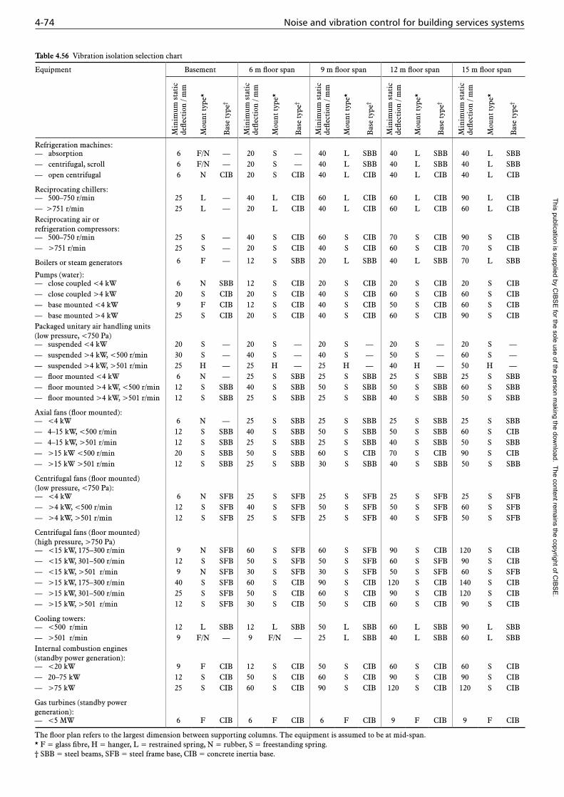
4-74 Noise and vibration control for building services systems
Table 4.56 Vibration isolation selection chart
Equipment Basement 6 m floor span 9 m floor span 12 m floor span 15 m floor span
Min
imum
sta
tic
defle
ctio
n / m
m
Mou
nt ty
pe*
Bas
e ty
pe†
Min
imum
sta
tic
defle
ctio
n / m
m
Mou
nt ty
pe*
Bas
e ty
pe†
Min
imum
sta
tic
defle
ctio
n / m
m
Mou
nt ty
pe*
Bas
e ty
pe†
Min
imum
sta
tic
defle
ctio
n / m
m
Mou
nt ty
pe*
Bas
e ty
pe†
Min
imum
sta
tic
defle
ctio
n / m
m
Mou
nt ty
pe*
Bas
e ty
pe†
Refrigeration machines:— absorption 6 F/N — 20 S — 40 L SBB 40 L SBB 40 L SBB— centrifugal, scroll 6 F/N — 20 S — 40 L SBB 40 L SBB 40 L SBB— open centrifugal 6 N CIB 20 S CIB 40 L CIB 40 L CIB 40 L CIB
Reciprocating chillers:— 500–750 r/min 25 L — 40 L CIB 60 L CIB 60 L CIB 90 L CIB— >751 r/min 25 L — 20 L CIB 40 L CIB 60 L CIB 60 L CIBReciprocating air or refrigeration compressors: — 500–750 r/min 25 S — 40 S CIB 60 S CIB 70 S CIB 90 S CIB— >751 r/min 25 S — 20 S CIB 40 S CIB 60 S CIB 70 S CIB
Boilers or steam generators 6 F — 12 S SBB 20 L SBB 40 L SBB 70 L SBB
Pumps (water):— close coupled <4 kW 6 N SBB 12 S CIB 20 S CIB 20 S CIB 20 S CIB— close coupled >4 kW 20 S CIB 20 S CIB 40 S CIB 60 S CIB 60 S CIB— base mounted <4 kW 9 F CIB 12 S CIB 40 S CIB 50 S CIB 60 S CIB— base mounted >4 kW 25 S CIB 20 S CIB 40 S CIB 60 S CIB 90 S CIBPackaged unitary air handling units (low pressure, <750 Pa)— suspended <4 kW 20 S — 20 S — 20 S — 20 S — 20 S —— suspended >4 kW, <500 r/min 30 S — 40 S — 40 S — 50 S — 60 S —— suspended >4 kW, >501 r/min 25 H — 25 H — 25 H — 40 H — 50 H —— floor mounted <4 kW 6 N — 25 S SBB 25 S SBB 25 S SBB 25 S SBB— floor mounted >4 kW, <500 r/min 12 S SBB 40 S SBB 50 S SBB 50 S SBB 60 S SBB— floor mounted >4 kW, >501 r/min 12 S SBB 25 S SBB 25 S SBB 40 S SBB 50 S SBB
Axial fans (floor mounted):— <4 kW 6 N — 25 S SBB 25 S SBB 25 S SBB 25 S SBB— 4–15 kW, <500 r/min 12 S SBB 40 S SBB 50 S SBB 50 S SBB 60 S CIB— 4–15 kW, >501 r/min 12 S SBB 25 S SBB 25 S SBB 40 S SBB 50 S SBB— >15 kW <500 r/min 20 S SBB 50 S SBB 60 S CIB 70 S CIB 90 S CIB— >15 kW >501 r/min 12 S SBB 25 S SBB 30 S SBB 40 S SBB 50 S SBB
Centrifugal fans (floor mounted) (low pressure, <750 Pa):— <4 kW 6 N SFB 25 S SFB 25 S SFB 25 S SFB 25 S SFB— >4 kW, <500 r/min 12 S SFB 40 S SFB 50 S SFB 50 S SFB 60 S SFB— >4 kW, >501 r/min 12 S SFB 25 S SFB 25 S SFB 40 S SFB 50 S SFB
Centrifugal fans (floor mounted) (high pressure, >750 Pa)— <15 kW, 175–300 r/min 9 N SFB 60 S SFB 60 S SFB 90 S CIB 120 S CIB— <15 kW, 301–500 r/min 12 S SFB 50 S SFB 50 S SFB 60 S SFB 90 S CIB— <15 kW, >501 r/min 9 N SFB 30 S SFB 30 S SFB 50 S SFB 60 S SFB— >15 kW, 175–300 r/min 40 S SFB 60 S CIB 90 S CIB 120 S CIB 140 S CIB— >15 kW, 301–500 r/min 25 S SFB 50 S CIB 60 S CIB 90 S CIB 120 S CIB— >15 kW, >501 r/min 12 S SFB 30 S CIB 50 S CIB 60 S CIB 90 S CIB
Cooling towers:— <500 r/min 12 L SBB 12 L SBB 50 L SBB 60 L SBB 90 L SBB— >501 r/min 9 F/N — 9 F/N — 25 L SBB 40 L SBB 60 L SBBInternal combustion engines (standby power generation):— <20 kW 9 F CIB 12 S CIB 50 S CIB 60 S CIB 60 S CIB— 20–75 kW 12 S CIB 50 S CIB 60 S CIB 90 S CIB 90 S CIB— >75 kW 25 S CIB 60 S CIB 90 S CIB 120 S CIB 120 S CIB
Gas turbines (standby power generation):— <5 MW 6 F CIB 6 F CIB 6 F CIB 9 F CIB 9 F CIB
The floor plan refers to the largest dimension between supporting columns. The equipment is assumed to be at mid-span. * F = glass fibre, H = hanger, L = restrained spring, N = rubber, S = freestanding spring. † SBB = steel beams, SFB = steel frame base, CIB = concrete inertia base.
This publication is supplied by CIB
SE
for the sole use of the person making the dow
nload. The content remains the copyright of C
IBS
E.

Vibration problems and control 4-75
resonance frequency of 4.5 Hz is required at mount static deflection of 12 mm.
The conclusions are that:
— required vibration isolation efficiency percentage will decrease as disturbing frequency decreases
— required vibration isolation efficiency percentage will increase as machine absorbed power increases
— required mount static deflection increases, and required mount natural frequency lowers, as disturbing frequency decreases.
Therefore when specifying vibration isolators for a typical project it would normally be possible to state that vibration isolator performance should conform to Table 4.56. Its deficiency is that no allowance is made for corrections to mount selections for structural characteristics (e.g. floors with a low stiffness) or for special isolation where unusual room conditions apply (e.g. studios, life sciences).
4.11.4.2 Relation between vibration at source and the associated structure
Simple vibration theory, as used above, assumes that the isolator is mounted on a solid narrow span or foundation, a condition that might be approached in a basement, or on a slab that is sufficiently stiff not to have any significant effect on mount selection. Table 4.56 makes a rule of thumb attempt to accommodate this. This would include any floor where the natural frequency of the slab would be no lower than fn = 30 Hz. The typical range for fn in floor slabs is from 4 Hz (low extreme) upwards.
However, floor spans have increased, quite commonly up to 10 m and beyond, and where plant is located on intermediate floors, or even at roof top level, the vibration characteristics of the support structure, might interact with the vibrations
of the plant, and/or the characteristics of the vibration isolators. Wherever long span, low spring rate, low natural frequency floors are encountered expert acoustic and structural engineering assistance should be sought. So far as vibration isolation is concerned there is no objective linear scale that defines structural weakness from one natural frequency to another. The only way this can be defined is in relation to the vibration design criterion; the disturbing frequency and power of the source; the natural frequency of the support system and structure; and the mount performance characteristics. These factors are addressed in the guidelines below. Failing this the basic mount selection listed or indicated in Tables 4.56 and 4.57 should be utilised. Severe conditions are usually self-evident and will mean that the following guidelines apply:
(a) The spring rate of the mounted machine should be not less than one tenth of the spring rate of the slab. So if a machine with an operating weight of 2400 kg is supported by 125 mm deflection mounts, then the machine mounted spring rate is 2400/125 = 19.2 kg/mm. The spring rate of the floor must therefore be not less than 192 kg/mm. Note that when this guideline indicates that higher mount static deflection is required than that indicated in Table 4.57 (as it often will) then that higher deflection should predominate in selecting the mount.
Alternatively, this guideline can be inverted:
(b) The static deflection of the mounted machinery should be not less than ten times the differential deflection of the slab (amount deflected under the machine load). If therefore the mounted machine deflection is 125 mm the slab differential deflection must not exceed 12.5 mm under the imposed machine load.
Table 4.57 Illustrating practical expectations for vibration isolation (reproduced courtesy of Ervin APL)
Machine power / kW
Vibration isolation efficiency (vie), static deflection (d) and mounting resonance frequency (fn) for stated lowest disturbing frequency (fd)
fd = 3.3 Hz fd = 7.5 Hz fd = 12.0 Hz
vie / % d / mm fn / Hz vie / % d / mm fn / Hz vie / % d / mm fn / Hz
0–0.9 42 65 2 72 20 3.5 83 12 4.61–9.9 42 65 2 88 40 2.5 83 12 4.6
10–49.9 64 85 1.7 92 65 2 93 25 350–99.9 74 105 1.5 95 85 1.7 97 65 2>100 78 125 1.4 96 105 1.5 98 85 1.7
fd = 15.0 Hz fd = 25.0 Hz fd = 33.0 Hz
vie / % d / mm fn / Hz vie / % d / mm fn / Hz vie / % d / mm fn / Hz
0–0.9 84 8 5.5 96 12 4.6 94 4 7.91–9.9 90 12 4.5 96 12 4.6 97 8 5.6
10–49.9 95 25 3.2 98 20 3.5 98 12 4.650–99.9 97 40 2.5 98 25 3.2 99 20 3.5>100 98 65 2.0 99 40 2.5 99 25 3.2
Notes:
(1) The disturbing frequency, fd, is usually the lowest speed of rotation
(2) The machine power is the absorbed power at the given speed of rotation, not the nominal rating or the absorbed power at a different speed
(3) d is the minimum vibration isolator static deflection under a given static load; where the input data is of doubtful provenance, it is frequently necessary to select, say, a 75 mm static deflection isolator to give a minimum static deflection of, say, 60 mm
(4) fn is the natural frequency of the isolator/mounted machinery as installed and levelled, and assuming the support structure and the machine base frame are of infinite stiffness and the minimum isolator static deflection is obtained
This publication is supplied by CIB
SE
for the sole use of the person making the dow
nload. The content remains the copyright of C
IBS
E.

4-76 Noise and vibration control for building services systems
(c) The the natural frequency of the isolated machine should be significantly lower than the natural frequency of the slab. Further, the natural frequency of the slab should be significantly higher than the disturbing frequency of the machine. Note that it is difficult to define firm limits and it is recommended that experienced specialists are consulted on such projects.
For less critical cases many vibration isolation manufac-turers have their own standard recommendations for mounts allowing for increased floor span, varying absorbed power levels, and particular kinds of equipment, which are generally satisfactory as they err on the side of safety (see for example Table 4.56).
There is another rule of thumb method for addressing less critical problems of vibration isolation interface with structures. This can be addressed in the same way as where coupling occurs between integral mounts installed within equipment, such as on fan/motor sections within an ahu, and the external mounts located between the equipment and the floor. The method is to add the actual static deflection of the fan/motor mounts to the theoretical required static deflection of the external mounts, e.g. if the integral mount d is 6 mm and the external mount d is 12 mm, then the final corrected external mount d will be 18 mm. In a similar way the mid-span differential floor deflection may be added to the theoretical external mount deflection to make allowance for any proximity between mount fn and floor fn. However this is unlikely to consistently yield the 10:1 machine deflection to slab deflection referred to above, and so this method should be used with caution.
Do not underestimate the significance of ‘weak’ plant room floors where the slab spring rate as indicated above might easily be say 192 kg/mm. This would call for a machine/mount spring rate of 19.2 kg/mm and a possible static deflection up to 125 mm. Clients should be encouraged to make plant room floors and other relevant floors, e.g. floors with significant fan coil unit load suspended, as stiff as possible.
For a more illustrative and specific guidance on the interface between vibration isolation and ‘weak’ structures refer to section 4.11.6.3 below.
4.11.4.3 Vibration rating for machinery
This was addressed briefly in section 4.11.3. It can be valuable to add include request such as:
‘Equipment will be properly statically and dynamically balanced at works, and certified accordingly. The stated performance duty of the equipment shall be such as to comply with a stable proportion of the machine’s operating curve. The significant individual component centres of gravity shall be shown, together with the overall equipment centre of gravity. The preferred support locations shall be shown, preferably with the vertical loads imposed. The overall dimensions of the machine and any associated skid shall be shown together with the specific dimensions of individual skid members.’
Machine fragility levels are best given as the maximum acceleration levels that can be withstood at a range of input frequencies between 3.0 Hz and 15.0 Hz without resulting in machine malfunction. Fragility levels only usually apply
where ordnance or seismic risk is evident, but can also apply for carriage/drop-shock, purposes.
4.11.5 Common types of vibration isolator
Figure 4.57 illustrates common types of vibration isolator.
4.11.5.1 General
A number of difficulties arise in the selection of vibration isolators. In particular, static deflection depends on vertical load, but this load is not always known accurately. The vertical load from the plant is either given by the equipment manufacturer or calculated from input data supplied by the manufacturer. Either way it is subject to error, often an underestimate. Additionally, anti-vibration mount (avm) suppliers add safety factors over and above any safety limit built-in to the isolator design. The avm supplier will not normally produce a bespoke mount, but offer the nearest standard one above the required carrying capacity. It is therefore important to make a distinction between minimum required static deflection and the rated static deflection that a mount gives when accurately loaded. A common example is the selection of nominal 30 mm deflection helical spring mounts to give not less than 25 mm static deflection.
4.11.5.2 Pad materials: flat, laminated and contoured
With some exceptions, pad materials are too unpredictable and limited in performance to be regarded as reliable vibration isolators. Their most popular, convenient, and successful role is as cheap and easily fitted sound separators, rather than vibration isolators. Elastomeric materials have inherent variability of elastic properties, which affect their performance. A column of elastomer will not compress uniformly, and will only deflect in proportion to its ability to bulge or distort under load, determined by the ‘shape factor’, which is given by:
Shape factor = area under load / area free to bulge
Thus, a circular disc of elastomeric will deflect somewhat less than a rectangular strip of equal thickness and equal surface area, under the same load. Generally, a high shape factor produces a stiff mount.
In order to avoid over-stress, a deflection limit on pads is 10–15% of the thickness. Reliable deflection is also compromised by the wide manufacturing tolerance, presently ±5%, allowed for moulded stiffness (related to Shore hardness). Further, the static and dynamic stiffness of a given elastomeric differ with batch, resulting in non-linear deflection. The mounted resonance frequency should not be determined from equation 4.41, although an approximation may be obtained by multiplying the result by 1.2. For preference, refer to individual manufacturers for information, but a distinction should be drawn between standard catalogue information and certified data. Much catalogue data will assume equation 4.41 is valid for elastomers which can be misleading. Trial design exercises will quickly demonstrate the limitations of pads as isolators. They are best regarded as low frequency noise separators, i.e. low frequency noise insulators, rather than vibration isolators.
This publication is supplied by CIB
SE
for the sole use of the person making the dow
nload. The content remains the copyright of C
IBS
E.
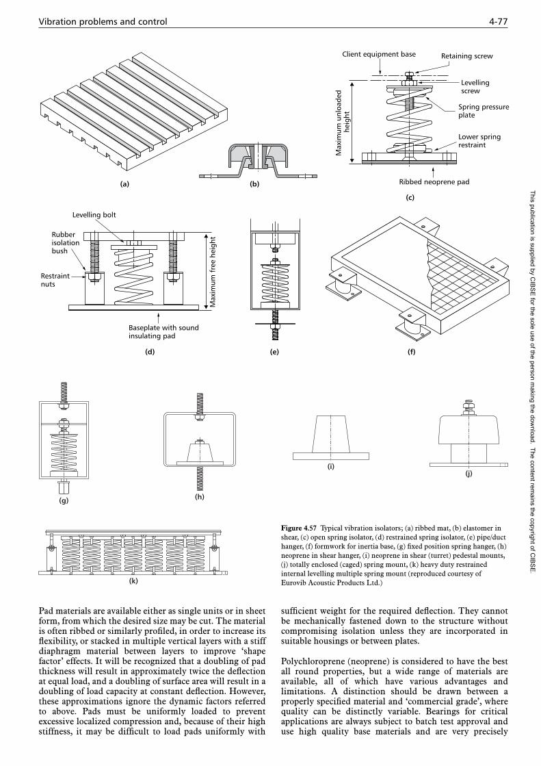
Vibration problems and control 4-77
Pad materials are available either as single units or in sheet form, from which the desired size may be cut. The material is often ribbed or similarly profiled, in order to increase its flexibility, or stacked in multiple vertical layers with a stiff diaphragm material between layers to improve ‘shape factor’ effects. It will be recognized that a doubling of pad thickness will result in approximately twice the deflection at equal load, and a doubling of surface area will result in a doubling of load capacity at constant deflection. However, these approximations ignore the dynamic factors referred to above. Pads must be uniformly loaded to prevent excessive localized compression and, because of their high stiffness, it may be difficult to load pads uniformly with
sufficient weight for the required deflection. They cannot be mechanically fastened down to the structure without compromising isolation unless they are incorporated in suitable housings or between plates.
Polychloroprene (neoprene) is considered to have the best all round properties, but a wide range of materials are available, all of which have various advantages and limitations. A distinction should be drawn between a properly specified material and ‘commercial grade’, where quality can be distinctly variable. Bearings for critical applications are always subject to batch test approval and use high quality base materials and are very precisely
Client equipment base
Ribbed neoprene pad
Max
imum
unl
oade
d he
ight
Retaining screw
Levellingscrew
Spring pressureplate
Lower springrestraint
Levelling bolt
Baseplate with soundinsulating pad
Max
imum
fre
e he
ight
Rubberisolationbush
Restraintnuts
(a) (b)
(c)
(d) (e) (f)
(g) (h)
(i)(j)
(k)
Figure 4.57 Typical vibration isolators; (a) ribbed mat, (b) elastomer in shear, (c) open spring isolator, (d) restrained spring isolator, (e) pipe/duct hanger, (f) formwork for inertia base, (g) fixed position spring hanger, (h) neoprene in shear hanger, (i) neoprene in shear (turret) pedestal mounts, (j) totally enclosed (caged) spring mount, (k) heavy duty restrained internal levelling multiple spring mount (reproduced courtesy of Eurovib Acoustic Products Ltd.)
This publication is supplied by CIB
SE
for the sole use of the person making the dow
nload. The content remains the copyright of C
IBS
E.

4-78 Noise and vibration control for building services systems
engineered products. For example, when elastomeric blocks are used in building bearings, all of the static and dynamic variables are taken into account, as a guaranteed maximum resonant frequency is required. Manufacturing techniques include compression moulding, injection moulding, extrusion and calendaring. Where pads or blocks are involved as building bearings, or as floating floors, they are always purpose-designed, or purpose-selected from very accurate data prepared for products of much higher quality than the everyday utility standard. Either way an acoustic specialist should be retained.
4.11.5.3 Elastomer-in-shear
These mounts suffer from the same fundamental limitations and unpredictable variables as do pads, but to a lesser degree. However, to achieve significant deflections without excessive column height, it has been common practice for some 50 years to install elastomers, at least partly, in shear. An example is conical turret mounts, with static deflections up to 10 mm. There is greater flexibility in shear than in compression, although most isolators use a combination of shear and compression. The most commonly claimed upper deflection limit is 12 mm, but 10 mm should be regarded as the practical maximum. Some engineers select at 12 mm d, assume they will only get 5 mm,and use the fn and vibration performance published for say 6 mm d, thus allowing for the anomalies discussed above.
For the approximate determination of resonant frequency, in the absence of manufacturers’ certified data, equation 4.41 may be used and the result multiplied by 1.2. The reason for the multiplier is to make allowance for internal damping, dynamic characteristics of the elastomer, and variability of Shore Hardness. As with pads and blocks, elastomer-in-shear mounts are most commonly associated with lighter loads and higher disturbing frequencies, but there are exceptions. These mounts are also available in hanger form, both on their own and in conjunction with helical springs. Unlike pads, elastomer-in-shear mounts can be fixed down without compromising the isolation. They are very commonly incorporated into fan and pump products by the equipment manufacturer.
These mounts are best viewed as simple, small dimension and inexpensive solutions to vibration problems where the disturbing frequencies are no lower than 20 Hz and the machine absorbed horsepower does not exceed 1.0 kW. In other words on small, light, equipment rotating at 1200 r/min and over.
4.11.5.4 Helical springs
The helical spring is the most commonly used, most reliable and most predictable device employed in vibration isolation. Springs differ from elastomer materials in that they deflect uniformly under increasing load and have equal static and dynamic stiffness, as required for equation 4.41. There are various mounting configurations including open, caged, enclosed and restrained. They are also available as pipe or duct hangers. When supplied in other than ‘open’ mode they can be damped or undamped. They are available in a wide range of load carrying capacities from kilograms to tonnes per isolator.
Typical deflections are 12, 15, 25 and 30 mm and provide a mounting frequency of up to about 3.0 Hz, and a vibration
isolation efficiency (vie) of up to 95%, but they are readily available in deflections up to 150 mm. Helical springs occasionally experience efficiency loss at higher machine frequencies due to wave propagation through the spring (especially in hanger mode) and this has led to the incorporation of elastomeric pads as vibration breaks. When in ‘open’ format it is good practice for the ratio between spring diameter and spring deflected height to be no less than 0.8:1.0 in order to promote spring stability. When enclosed, caged or restrained this relationship is clearly less important, although good spring design should always preclude buckling and other forms of instability.
If springs are to be fixed at their upper or lower ends, methods other than welding, which affects temper, should be sought. Springs are generally designed with up to 50% overload potential, but the overload percentage will diminish as the rated load increases, otherwise the spring will reach unreasonable dimensions. Load range can be increased by ganging springs in parallel, leading to restrained spring mounts of up to 8 tonnes load at up to 150 mm static deflection.
4.11.5.5 Inertia bases
A spring supported base supporting mechanical equipment, is referred to as an inertia base. A steel base frame without spring support is a known as a skid, and concrete bases without springs underneath are referred to as plinths or ‘housekeeping pads’. Displacement forces from the mechanical ‘driver’ have to overcome the additional inertia provided by the inertia base. This is very effective where there are two or more drivers, perhaps at differing speeds of rotation, as with a motor and a fan or a motor and a pump. The base may be a bolted or welded steel concrete pouring frame, or a cast concrete base in a timber or metal former, the former having first been fitted on the underside with pads or mounts. Inertia bases can be used to provide additional mass per spring, thus increasing static deflection and reducing the resonant frequency of a supported system. However, care should be taken that the additional mass does not cause problems to the structure. The additional mass is useful in lowering the centre of gravity of the supported system and in providing resistance to lateral and axial forces. A typical inertia base consists of a steel form, which is filled with concrete to give the mass.
Support brackets for vibration isolators are usually attached to the base. A larger base is used to provide a platform for a number of items of equipment, e.g. run and standby pumps, which cannot conveniently be supported individually. Most pumps are very conveniently mountable on inertia bases, which also give the advantages of improved vibration isolation. Spring mounted concrete pouring frames are available in flat pack form for bolted on-site assembly. These have the advantage of lightweight shipping and site handling and their final location in the plant room can be chosen and adjusted before pouring the concrete. Advice should be sought before finalizing the design of an inertia base. Where size and weight permit, bases can be delivered pre-assembled and even pre-concrete-filled.
The rule of thumb for the ratio of masses of the base and the supported equipment is 1.5:1.0 for most conventional equipment, including pumps, but could rise to 5:1 for equipment with large lateral out-of-balance forces such as high pressure blowers, where there are high static and velocity pressures.
This publication is supplied by CIB
SE
for the sole use of the person making the dow
nload. The content remains the copyright of C
IBS
E.

Vibration problems and control 4-79
It has become common for the fan and motor section of air handling units (ahus) to be internally isolated using a lightweight steel inertia base, spring mounts and one or more flexible duct connectors. While this arrangement can work effectively, it is a general solution and for more critical applications it is preferable to have the fan/motor section mounted rigidly and to isolate the whole ahu from the structure, if necessary incorporating steel rails to tie the whole assembly together. This has the added advantage of presenting the whole of the unit as inertia to the ‘driver’.
4.11.5.6 Flexible pipe connectors
Although quite short, typically 150 mm flange-to-flange, these give flexibility to prevent vibration forces in anchored pipes bypassing the isolators and also take up strains from minor misalignments. They are not to be confused with expansion joints, which are specialist products employed for different purposes. They are available in a range of reinforced elastomers, and with flanged or screwed connections. For high pressures or other risk of displacement they are available with isolated restraint rods. Reliable data for their isolation efficiency is not available but it is generally believed to be good practice to install them, for example, on any pump flow and return. Spring hangers will still be required, especially where pipe work is fixed to structures directly adjacent to occupied areas. They are not to be confused with hoses, some of which are properly rated for noise and vibration isolation (BS EN 1736 (BSI, 2008b)). A typical pump installation reflecting good vibration isolation practice will consist of a spring inertia base, a flow and return flexible pipe connector, and perhaps four spring hangers.
4.11.5.7 Flexible duct connectors
Used as a vibration break, particularly between the fan and its duct, they can be of circular or rectangular section. The recommended length of 250–300 mm is sufficient to allow 150 mm of slack between the two coupled ducts. They are normally made from organic or synthetic canvas impreg-nated with neoprene or another sealing elastomer, but are also available in a range of alternative materials with varying acoustic and fire ratings. The better models are provided with their own integral fabric flanges and a matching metal flange. They can also be fitted directly to coupling ductwork by jubilee clips. Reliable data for vibration isolation performance is not available but their use signifies good practice, although duct isolation hangers may still be necessary.
4.11.5.8 Isolation hangers
These are used for ducts and pipes. Where plant rooms directly adjoin occupied areas and especially where ‘weak’ structures are present, it is essential that pipe work and ductwork are isolated from the structure. The flexible element may be either helical spring or elastomer or a combination of these. A good design of hanger will have a spring diameter to height ratio of 0.8:1.0, large clearance holes which are grommet and bush protected, an elastomeric element to preclude high frequency bypass, and a restraint cross-bar to enable the load to be taken and pipes to be levelled prior to the spring being actually loaded. Doing this prevents overloading the springs and avoids erratically levelled pipe or the need for retro-fitting of hanger. Where detailed pipe and duct coordinated services drawings are
available, together with adequate architectural and structural detail, hangers can be selected and located in advance. Current practice is for pipe work to be installed ‘rigid’ on standard studding, but leaving enough vertical room for the hangers to be cut-in later, thus ensuring their accurate selection from a site survey. Increasing machine powers, weaker slabs and developing environmental awareness, are putting greater emphasis on the inclusion of spring hangers in plant rooms. Spring hangers are essential where acoustic ceilings are installed. Spring hangers are very important where deep core occupied spaces incorporate large numbers of fan coil units. Frequently there is a ‘weak’ floor from which units are suspended. If fan coil units are not vibration isolated their disturbing frequency is likely to be in resonance with the floor fn. Pipe and ductwork flex connections should also be installed.
4.11.5.9 Air springs
The use of helical steel springs requires increasing amounts of static deflection as the required mounted natural frequency is reduced. Assuming a rigid structure, from equation 4.41, a natural frequency of 1.4 Hz requires a static deflection of 125 mm. To achieve an actual static deflection of 125 mm, helical springs would be designed for 150 mm static deflection, due to the input variables, which probably represents the upper limit for convenient helical spring mount design, especially where very light or very heavy loads are concerned. Air springs operate in a different way and achieve natural frequencies of 1 Hz (equivalent to 250 mm of static deflection). They are basically air-filled reinforced rubber cushions with a valve controlling the internal air pressure, giving variation of the load carrying capacity and natural frequency. They require regular inspection and maintenance, including a constant air supply. Air springs are effective where high levels of isolation are required, e.g. for an electron microscope, taking up much less space than their helical spring counterparts. However for general purposes they are not as convenient or competitive as elastomers and helical springs, which will be more frequently encountered by the building services engineer.
4.11.5.10 Floating floors
The maximum difference in noise level obtainable from a homogenous construction is about 50 dB, particularly at lower frequencies. No matter how much design input and installation care is taken to optimise the mass, the quality of the construction and avoidance of leaks through air gaps, the level difference is controlled by flanking paths. The purpose of floating floors is the minimisation of flanking paths and the introduction of an isolating air space.
While there is no reason why floating floors should not be designed for vibration isolation, this can lead to difficulties, particularly from differential plant loading and it is for this reason that the floating floor is more often considered as an acoustical treatment. Floating floors are designed with natural frequencies down to e.g. 6 Hz, which is still comfortably within the range of elastomer-in-shear isolators, while for higher resonant frequencies, e.g. 10–15 Hz, pads and quilts can be used. The simplest floating floor is concrete laid onto a resin bonded mineral wool mat, such that the mat has only a small deflection. More complex systems use an array of pads covered by formwork, onto which the concrete is poured. Some spring
This publication is supplied by CIB
SE
for the sole use of the person making the dow
nload. The content remains the copyright of C
IBS
E.

4-80 Noise and vibration control for building services systems
systems have a jack-up capability whereby mounts are installed ‘solid’ to facilitate concrete casting, and are later jacked-up and levelled, using pre-cast holes in the top of the slab, thus providing the necessary clearance between the cast float and the substrate. It is normal, where the floating floor is in the plant room, to regard the floating floor as a noise insulator, and to cast separate housekeeping pads to the substrate from which to mount the usual spring inertia bases to support equipment. The floating floor is thus ‘dressed’ to the room and plant base perimeters using neoprene resilient strip.
Design of a floating floor must take the following into consideration:
— the additional mass of the floating floor on the structural floor via the mounts or pads
— the additional mass of any light plant that might be directly mounted on the float
— the additional mass of any false walls or ceiling that might be involved and mounted on the float
— the need for isolated drain-down points
— the precise number, distribution, and capacity of mounts
— the importance of levelling.
Specialist advice must be sought in the design of a floating floor.
4.11.5.11 Structural bearings
These are used to isolate whole buildings from earthquake or shock, or from excessive low frequency noise such as nightclubs and underground railways. Construction of the bearings is often basically elastomeric pads or blocks, sometimes built up as a multiple sandwich construction between steel plates although springs may be used. This is a specialised area involving high quality base material and very precise engineering, for which expert help must be sought, omnidirectional restraint being essential.
4.11.6 Practical examples of vibration isolation
4.11.6.1 General observations
Degrees of freedom
There are six degrees of freedom manifested when an object free-to-move is subject to a force. They are illustrated in Figure 4.58 and are as follows:
— Z-axis: up/down
— X-axis: side/side
— Y-axis: fore/aft
— plus the three rotational directions about these axes.
The dominant force in most building services plant is vertically downward in the Z-axis, and satisfying this requirement will normally satisfy forces in other directions by default. The exceptions tend to be the situations where inertia bases are incorporated and this controls motion
(though not forces) in other directions, including rocking modes. Typical uses of inertia bases are for motor/pump assemblies, fan/motor assemblies, compressors, plant with high centre of gravity, large diameter industrial blowers.
Number and location of mounts
Generally one of the three following situations will apply:
— mount positions, and full associated data are provided by the supplier
— mount positions and limited data are provided
— limited data and no mount positions are given.
Depending upon the situation the following options in regard to the number and location of mounts are available:
(1) Work in either two or three dimensions in regard to the centre of gravity. Other than in exceptional circumstances where specialists are involved, one will use the horizontal centre of gravity only.
(2) Support at equal centres from the horizontal centre of gravity. In a six or more mount selection, this will provide equal loading on all mounts except for the extremities which will be half-load.
(3) Support at equal centres about the horizontal centre of gravity. This is the mathematical and engineering ‘ideal’ situation where all mounts are at equal centres and equal loads, but the absence of mounts at the corners is sometimes impractical. You can support with all mounts at equal loads and mounts will be centred accordingly.
Note: unequal centres and unequal loads should be avoided. In every case mounts should not be at greater than 2000 mm centres or more than 600 mm from the end of the base or skid.
The design should ensure, in order of preference and engineering judgment:
— equal mount centres and equal mount loads
— equal stated loads but differential centres
— equal centres but unequal loads.
Longitudialinertia force(Y-axis)
Verticalinertia force(Z-axis)
Yawingcouple
Pickingcouple
Rockingcouple
Horizontaltransfer inertiaforce (X-axis)
Figure 4.58 The six degrees of freedom of a rigid body
This publication is supplied by CIB
SE
for the sole use of the person making the dow
nload. The content remains the copyright of C
IBS
E.
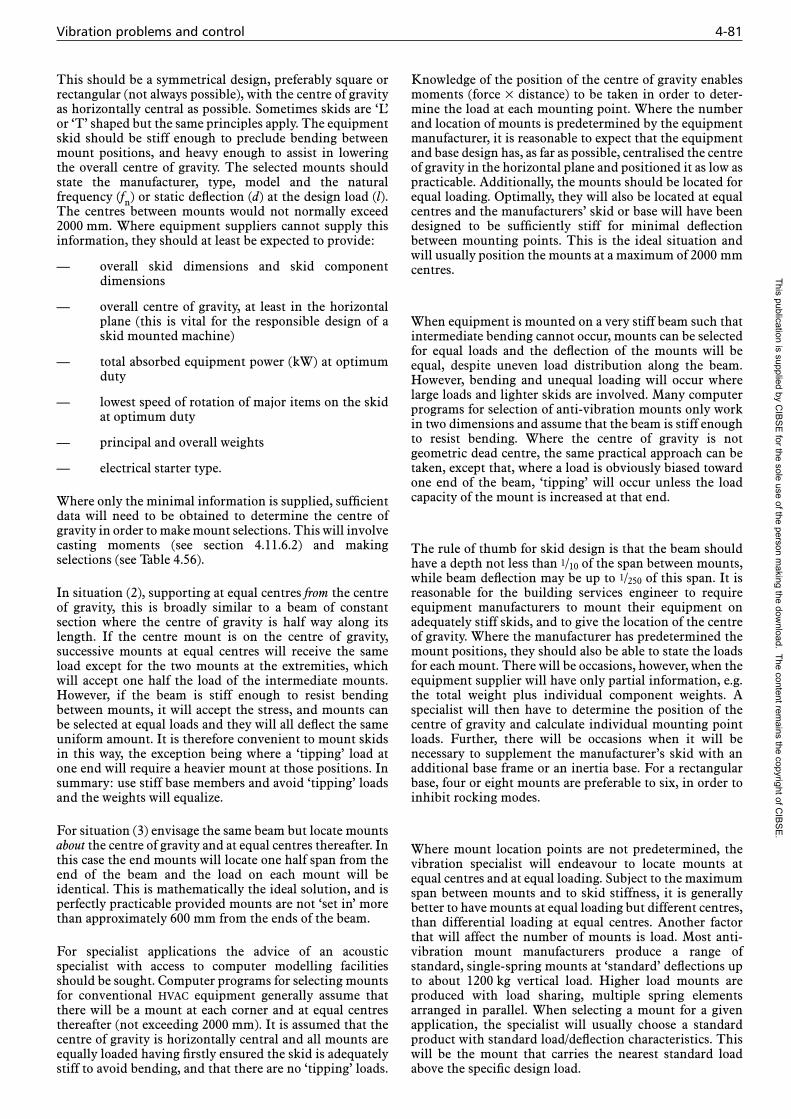
Vibration problems and control 4-81
This should be a symmetrical design, preferably square or rectangular (not always possible), with the centre of gravity as horizontally central as possible. Sometimes skids are ‘L’ or ‘T’ shaped but the same principles apply. The equipment skid should be stiff enough to preclude bending between mount positions, and heavy enough to assist in lowering the overall centre of gravity. The selected mounts should state the manufacturer, type, model and the natural frequency (fn) or static deflection (d) at the design load (l). The centres between mounts would not normally exceed 2000 mm. Where equipment suppliers cannot supply this information, they should at least be expected to provide:
— overall skid dimensions and skid component dimensions
— overall centre of gravity, at least in the horizontal plane (this is vital for the responsible design of a skid mounted machine)
— total absorbed equipment power (kW) at optimum duty
— lowest speed of rotation of major items on the skid at optimum duty
— principal and overall weights
— electrical starter type.
Where only the minimal information is supplied, sufficient data will need to be obtained to determine the centre of gravity in order to make mount selections. This will involve casting moments (see section 4.11.6.2) and making selections (see Table 4.56).
In situation (2), supporting at equal centres from the centre of gravity, this is broadly similar to a beam of constant section where the centre of gravity is half way along its length. If the centre mount is on the centre of gravity, successive mounts at equal centres will receive the same load except for the two mounts at the extremities, which will accept one half the load of the intermediate mounts. However, if the beam is stiff enough to resist bending between mounts, it will accept the stress, and mounts can be selected at equal loads and they will all deflect the same uniform amount. It is therefore convenient to mount skids in this way, the exception being where a ‘tipping’ load at one end will require a heavier mount at those positions. In summary: use stiff base members and avoid ‘tipping’ loads and the weights will equalize.
For situation (3) envisage the same beam but locate mounts about the centre of gravity and at equal centres thereafter. In this case the end mounts will locate one half span from the end of the beam and the load on each mount will be identical. This is mathematically the ideal solution, and is perfectly practicable provided mounts are not ‘set in’ more than approximately 600 mm from the ends of the beam.
For specialist applications the advice of an acoustic specialist with access to computer modelling facilities should be sought. Computer programs for selecting mounts for conventional hvac equipment generally assume that there will be a mount at each corner and at equal centres thereafter (not exceeding 2000 mm). It is assumed that the centre of gravity is horizontally central and all mounts are equally loaded having firstly ensured the skid is adequately stiff to avoid bending, and that there are no ‘tipping’ loads.
Knowledge of the position of the centre of gravity enables moments (force × distance) to be taken in order to deter-mine the load at each mounting point. Where the number and location of mounts is predetermined by the equipment manufacturer, it is reasonable to expect that the equipment and base design has, as far as possible, centralised the centre of gravity in the horizontal plane and positioned it as low as practicable. Additionally, the mounts should be located for equal loading. Optimally, they will also be located at equal centres and the manufacturers’ skid or base will have been designed to be sufficiently stiff for minimal deflection between mounting points. This is the ideal situation and will usually position the mounts at a maximum of 2000 mm centres.
When equipment is mounted on a very stiff beam such that intermediate bending cannot occur, mounts can be selected for equal loads and the deflection of the mounts will be equal, despite uneven load distribution along the beam. However, bending and unequal loading will occur where large loads and lighter skids are involved. Many computer programs for selection of anti-vibration mounts only work in two dimensions and assume that the beam is stiff enough to resist bending. Where the centre of gravity is not geometric dead centre, the same practical approach can be taken, except that, where a load is obviously biased toward one end of the beam, ‘tipping’ will occur unless the load capacity of the mount is increased at that end.
The rule of thumb for skid design is that the beam should have a depth not less than 1/10 of the span between mounts, while beam deflection may be up to 1/250 of this span. It is reasonable for the building services engineer to require equipment manufacturers to mount their equipment on adequately stiff skids, and to give the location of the centre of gravity. Where the manufacturer has predetermined the mount positions, they should also be able to state the loads for each mount. There will be occasions, however, when the equipment supplier will have only partial information, e.g. the total weight plus individual component weights. A specialist will then have to determine the position of the centre of gravity and calculate individual mounting point loads. Further, there will be occasions when it will be necessary to supplement the manufacturer’s skid with an additional base frame or an inertia base. For a rectangular base, four or eight mounts are preferable to six, in order to inhibit rocking modes.
Where mount location points are not predetermined, the vibration specialist will endeavour to locate mounts at equal centres and at equal loading. Subject to the maximum span between mounts and to skid stiffness, it is generally better to have mounts at equal loading but different centres, than differential loading at equal centres. Another factor that will affect the number of mounts is load. Most anti-vibration mount manufacturers produce a range of standard, single-spring mounts at ‘standard’ deflections up to about 1200 kg vertical load. Higher load mounts are produced with load sharing, multiple spring elements arranged in parallel. When selecting a mount for a given application, the specialist will usually choose a standard product with standard load/deflection characteristics. This will be the mount that carries the nearest standard load above the specific design load.
This publication is supplied by CIB
SE
for the sole use of the person making the dow
nload. The content remains the copyright of C
IBS
E.

4-82 Noise and vibration control for building services systems
Types of mount
Pads and elastomer-in-shear mounts are normally used for light loads and small machine power. Pads and blocks are useful ‘sound separators’ but are not an effective vibration isolator, other than when specially designed and selected, e.g. bearings, floating floors. Elastomer-in-shear has its lowest dynamic natural frequencies in the region of 6 Hz which will give adequate vibration isolation efficiency (vie) for disturbing frequencies down to about 1000 r/min (17 Hz), depending upon machine power and location. A maximum power of 1 kW and a minimum speed of 1200 r/min (20 Hz) is a reasonable guide. Although such mounts are available for high loads, the maximum recom-mended load per mount is 180 kg. These mounts should never be exposed to loads in extension, nor any significant lateral load without the approval of the manufacturer.
Commercial grade neoprene can be a good all-round choice of elastomer for plant room use, but due regard must be given to the location and function of adjoining spaces. These mounts are sometimes designated ‘single deflection’, meaning deflections up to 6 mm maximum, and ‘double deflection’ for up to 12 mm deflection. Elastomer-in-shear mounts, particularly the cheaper ones, do not normally incorporate levelling devices without reliance on long fixing screws and locking nut arrangements. However, because of the limited deflection, any differential loading will not result in undue out-of-level problems. As with all plant mounting operations, however, one should ensure that the initial plant base location is levelled before installation.
For applications involving machinery in excess of 1 kW absorbed power and an fd below 1200 r/min (20 Hz), helical steel spring mounts should normally be selected. The simplest of these is the open spring, which is typically restricted to operations where there are no significant differential loads (e.g fluid drain-down, or excessive wind or other lateral loads) which would require caged, enclosed or restrained spring mounts. It is often considered that open spring mounts are horizontally unstable, but better models ensure that the outer coil diameter is no less than 0.8×the deflected height, thus ensuring a very stable support that will satisfactorily accept horizontal forces up to two thirds of the rated vertical load. However, given the levels of investment that can depend on this product, it is important to verify this.
Properly selected and applied, a simple and inexpensive open spring mount (which will have a nominal 30 mm static deflection capacity in order to provide not less than 25 mm static deflection (fn = 3.0 Hz) at loads of up to 1000 kg) will probably suit up to 90% of most typical hvac applications. However, there will be occasions where the use of restrained heavy duty mounts, which provide restraint in six directions, will be required. They will typically incorporate elastomeric snubbers and bushes in order to preclude metal-to-metal contact and add damping. Fully enclosed spring mounts are also available and are useful for total weather protection, and also incorporate damping. The cast ‘open caged’ spring mount is now tending towards obsolescence.
A significant advantage of restrained spring mounts and hangers is that they can provide preset operating heights. This is especially important for hangers.
4.11.6.2 Determination of loads for a mounted system
The following example shows step-by-step calculations for loads for a system mounted at four points. Other procedures, generalised formulae and computer programs may also be used. The formula could be adapted to select four or more points at equal load but the and extra cost may prove unsatisfactory. In practice (as described above), dividing the total load by six and selecting six mounts at equal centres from the base centre line, will be effective (provided that the base is stiff enough not to bend, and there is no significant tipping load at one end). Note that the mounts would be height adjustable and also carry weight safety margins. Nonetheless the procedure as given is correct and the methods given are applicable to determination of the springs required for a variety of isolated systems such as pumps, fans or air handling units. Large systems, such as floating floors, cooling towers and whole buildings, require special techniques, some of which are discussed elsewhere in this section.
Example 1: fan and motor combination loads
The input data for a single fan and motor mounted on a rigid frame in the following example, is as follows:
— weight of fan: 21 kg
— weight of motor: 38 kg
— weight of frame: 12 kg
— frame dimensions: 1000 mm (L) × 550 mm (W) × 150 mm (D)
— operating speed: 900 r/min (15 Hz)
— presumed vibration isolation efficiency: 95%.
The positions of the centres of gravity of the fan and motor will have been provided by the manufacturer or determined separately, and are as shown in Figure 4.59.
The centre of gravity of the combination is on the line joining their separate centres of gravity (CG1 and CG2). The length of this line (T) is given by:
T = √ (L22 + W2
2) = √ (6002 + 2202) = 639 mm
The position of the centre of gravity of the combination on the line joining their separate centres of gravity is then given by moments around B as in Figure 4.60.
Hence:
59 X = 38 (X + Y) = 38 × 639
Leading to:
X = 411.6 mm and Y = 227.4 mm
It is now necessary to determine the weight distribution of the fan and motor at the corners of the frame, where the mountings will be located. The weight of the frame itself is divided equally between the corner supports.
The position of the fan/motor centre of gravity with respect to the edges of the frame is obtained by first determining distances L2′ and W2′ as in Figure 4.61. From consideration of the triangles it follows that L2′ = 214 mm and W2′ = 78.3 mm.
This publication is supplied by CIB
SE
for the sole use of the person making the dow
nload. The content remains the copyright of C
IBS
E.

Vibration problems and control 4-83
The centre of gravity of the combination in the horizontal plane is then determined as shown in Figure 4.62:
— distance from side AD of frame = L1 + L2
= 250 + 214 = 464 mm
— distance from side BC of frame = 536 mm
— distance from side DC = W1 + W2
= 150 + 78 = 228 mm
— distance from side AB = 322 mm
(As vertical motion only is assumed, the height of the centre of gravity is not considered).
The load sharing between sides AD and BC is obtained by a similar process to that shown in Figure 4.60. Hence:
— load carried on side BC = (464 / 1000) × 59
= 27.4 kg
giving:
— load carried on side AD = 31.6 kg.
In a similar manner, the distribution of load between points B and C is given by:
— load at B = (228 / 550) × 27.4 = 11.4 kg
giving:
— load at C = 16 kg
— load at D = (322 / 550) × 31.6 = 18.5 kg
giving:
— load at A = 13.1 kg
In addition to these loads, each support point carries one quarter of the 12 kg weight of the frame.
Therefore, total loads are 16.1 kg at A, 14.4 kg at B, 19 kg at C and 21.5 kg at D. However, it is advisable to add a safety margin of 15–20% to the calculated loads, to allow for error in input data.
The isolation efficiency required is 95%. From Table 4.57, standard 25 mm deflection mounts, chosen for appropriate load carrying, will be suitable.
An alternative method for determining the distribution of load to four support points for a known centre of gravity location via percentages is shown in Figure 4.63 below. For instance, the load transferred to the four corner support points for a centre of gravity located at the highlighted position (22, 8, 58, 12) will be distributed in the following proportions: 22% of the weight at corner A, 8% at corner B, 58% at corner C and 12% at corner D.
4.11.6.3 Mounting specific plant items and overall guidance
The example provided above can be applied to many items encountered by the building services engineer. Large plant may require additional mounting points which, for very heavy plant, may need to be chosen in relation to positions of support columns in the building.
A B
59 kg38 kg 21 kg
Y
T
X
Figure 4.60 Example 1: Position of centre of gravity of combination on line joining centres of gravity of fan and motor
W3
W2W
W1
W1 = 150 mmW2 = 220 mmW3 = 180 mm W1 = W1 + W2 + W3 = 550 mm
L1 = 250 mmL2 = 600 mmL3 = 150 mm L1 = L1 + L2 + L3 = 1000 mm
Motor FanCG2
CG1
L1 L2
LL3
Figure 4.59 Example 1: Plan dimensions showing position of fan and motor
Motor
Fan
220
411·6
227·4
600
W2'
L2'
Figure 4.61 Example 1: Location of centre of gravity of combination
Figure 4.62 Example 1: Position of centre of gravity of combination with respect to frame
BA
CG
CD
536 mm464 mm
228 mm
322 mm
This publication is supplied by CIB
SE
for the sole use of the person making the dow
nload. The content remains the copyright of C
IBS
E.

4-84 Noise and vibration control for building services systems
Further to this, interaction between the machine rotational speeds and any natural floor or even ground resonances will need to be considered. This will lead to a simplistic selection chart including floor span, isolator type, static deflection, and support base type.
The following sections consider some specific problems, solutions and overall selection guidance.
Mounting heavy plant on isolator rails
Cooling towers are considered, by way of example, but the principles are applicable to mounting any large item of plant on isolator rails, e.g. high capacity air handling units; diesel generators.
Traditionally, cooling towers were located either unmounted in non-critical locations, or sound-separated by pad/strip isolators. In some cases the fan/motor section alone, would be vibration isolated. As requirements became more demanding, isolated rail systems were developed for these and other large plant, whereby a pair of toe-down support channels was fitted along the length of the base of the tower with a nest of helical isolation springs. Isolation for equip-ment connected to the tower was provided by flexible pipe connectors, duct flexible connectors on forced draught fan discharges and, perhaps, some on-board isolation for the pump. The received wisdom in regard to deflection limit was generally 25 mm, which worked well and, in many instances, is still effective.
The use of cooling towers has declined but they are still encountered in both closed and open-circuit form, especially where very large condenser loads are required.
In the more serious cases large office blocks may have one or more cooling towers located at roof level, served by induced draught axial flow, or centrifugal forced draught fans. Multiple fans with a total absorbed power of 30 kW, and with a pump at perhaps a further 5 kW may be used. The power (thermal) rating for these towers can be as high as 3 MW and the operating weight 15 tonnes. Complications typically arise from:
— inverter speed control, typically 800 r/min (12 Hz) and down to around 130 r/min (approximately 2 Hz).
— a weak roof with a critical space, e.g. directors’ suite, immediately beneath
— cooling towers of modern monocoque construction, with a ‘weak’ base that do not allow direct mounting, but are designed and sold requiring some form of additional base frame and mounts, the design for which will depend upon the chosen location.
The static deflection will be determined by the required vie at the optimum duty (usually one of the higher speeds) plus any additional static deflection to avoid coupling with the natural frequency of a weak roof. The speed at optimum duty is almost always the most critical, because at lower speeds per the Fan Laws, there is a very substantial reduction in absorbed power due to reduced rotational forces. Using Table 4.57 a disturbing frequency (fd) of 800 r/min (13.3 Hz) and absorbed power 30 kW indicates
90 10 80 20 70 30 60 40 50 50 40 60 30 70 20 80 10 900 0 0 0 0 0 0 0 0 0 0 0 0 0 0 0 0 0
90 100 0
80 200 0
70 300 0
60 400 0
50 500 0
40 600 0
30 700 0
20 800 0
10 900 0
90
10
9
8
7
6
5
4
3
2
1
0
010 0
83 77 3
73 177 3
64 266 4
54 366 4
45 455 5
36 544 6
26 644 6
17 733 7
7 833 7
00
80 020 0
73 77 3
67 1313 7
58 2212 8
49 3111 9
40 4010 10
31 499 11
22 588 12
13 677 13
7 733 7
00
70 030 0
64 626 4
58 1222 8
52 1818 12
43 2717 13
35 3515 15
27 4313 17
18 5212 18
12 588 22
6 644 26
00
60 040 0
54 636 3
49 1131 9
43 1727 13
39 2121 19
30 3020 20
21 3919 21
17 4313 27
11 499 31
6 544 36
00
50 050 0
45 5 40 10 35 15 30 20 25 25 20 30 15 35 10 40 5 4545 5 40 10 35 15 30 20 25 25 20 30 15 35 10 40 5 45
00
40 060 0
36 454 6
31 949 11
27 1343 17
21 1939 21
20 2030 30
19 2121 39
13 2717 43
9 3111 49
4 366 54
00
30 070 0
26 464 6
22 858 12
18 1258 18
17 1343 27
15 1535 35
13 1727 43
13 1818 52
8 2212 58
4 266 64
00
20 080 0
7 30 0
13 70 0
12 80 0
11 90 0
10 100 0
9 110 0
8 120 0
7 130 0
3 77 73
00
10 090
9010
8020
7030
6040
5050
4060
3070
2080
10900
7 383 7
7 373 17
6 464 26
6 454 36
5 545 45
4 636 54
4 620 64
3 717 73
3 77 83
00
A B
DC
Figure 4.63 Support points for a known centre of gravity by percentage
This publication is supplied by CIB
SE
for the sole use of the person making the dow
nload. The content remains the copyright of C
IBS
E.

Vibration problems and control 4-85
required isolation on a rigid slab to at least 93% vie, which requires a static deflection (d) of 25 mm. The spring natural frequency is 3.0 Hz. The importance of the slab stiffness is not so much a function of its deflection under its own load, but rather any additional deflection created by the equipment load, i.e. the slab spring rate.
The slab spring rate is compared with the mount spring rate, where the mount spring rate needs to be not more than 1/10 of the slab spring rate in order to separate the two resonant frequencies. The mounted machine deflection needs to be 10 times the slab differential deflection. In this example slab differential deflection is not known, but assuming it is 10 mm then the mount static deflection must be 10 times greater or 100 mm (very often encountered in contemporary roof top cooling tower installations). As a final check, ensure that the natural frequency of the mount does not coincide with the natural frequency of the slab (information obtained from the structural engineer) and the natural frequency of the slab does not coincide with the machine disturbing frequency. The most obvious measure, if either should occur, is to further increase the mount static deflection and hence the vie. For the present example, assuming an additional slab deflection under load of 10 mm, the design static deflection of the mounts is increased from 25 mm to 100 mm, giving a spring natural frequency of 1.5 Hz.
If the floor deflects an additional 10 mm under a load of, say, 15 tonnes, the floor spring rate is 1500 kg/mm and the mount spring rate needs to be not more than 150 kg/mm. In practice, because of the input variables and spring selection and optimisation, the spring selection is preferred as nominal 125 mm static deflection mounts to achieve in situ deflection of not less than 100 mm. Current rooftop applications indicate that static deflections of nominal 75 mm are common and up to 125 mm is not unusual as a result of the combinations of high machine power, low rotational speeds, critical locations and weak roofs.
This is represented in Figure 4.64 which shows the preferred ratios of an isolated machine interface with a wide span floor where:
— machine fn at d = 100 mm: with no damping zero and infinitely stiff structure, fn = 1.58 Hz
— machine and support frame mass = 2000 kg
— machine disturbing frequency (fd) = 30 Hz
— machine mounted static deflection (d) = 100 mm
— machine spring rate (k) = 2000/100 = 20 kg/mm
— slab additional deflection attributable to machine mass = 10 mm
— slab spring rate (k) = 2000/100 = 200 kg/mm
— ratio of floor spring rate to spring rate mounted machine = 200:20 (10:1), which complies with the 1/10 rule described above
— ratio of mounted machine static deflection to floor additional deflection = 100:10 (10:1), which complies with the 1/10 rule described above.
The engineer will also need to avoid resonance between total slab fn and mounted machine fn; and slab fn and machine fd. Where plant is mounted on obviously ‘weak’ floors with high spans and low fn’s the engineer should always refer to an acoustic specialist and a structural engineer with relevant experience. Calculations become more complex where multiple plant is located on a single floor.
It is usual to arrange two or three vibration isolated parallel steel rails, laid on the roof or other flat surface, on which to support the plant. They usually consist of a toe-down channel above a heavy flat rail, separated but connected by a series of heavy duty restrained spring mounts. The rails should extend to the full dimensions of the base, and are drilled to allow the plant to be mechanically fixed to the housekeeping pad, and to accept the requisite number of restrained spring mounts. Because of difficulty in accessing levelling screws and also in providing a clear upper support surface on the mounts, internal levelling mounts are usually provided. Depending on the rail profile, the flanges of the toe-down channels may have to be provided with cut-outs to allow access to the levelling screws. The number of mounts is determined by the total load required and the permitted maximum span between mounts, which in turn will be influenced by structural column centres and the structural engineer’s proposals for supporting point loads from the mounts. Typical rail sections are 200 mm × 75 mm
2000 kgfd = 30 Hz
Machine fn @ d = 100 mm;Damping zero and infinity stiff structure, fn = 1·58 Hz
10 mm
100 mm
Notationalequivalentto mid span10 mm d
Notationalequivalentto mid span10 mm d
Figure 4.64 Isolated machine interface with a wide span floor
This publication is supplied by CIB
SE
for the sole use of the person making the dow
nload. The content remains the copyright of C
IBS
E.
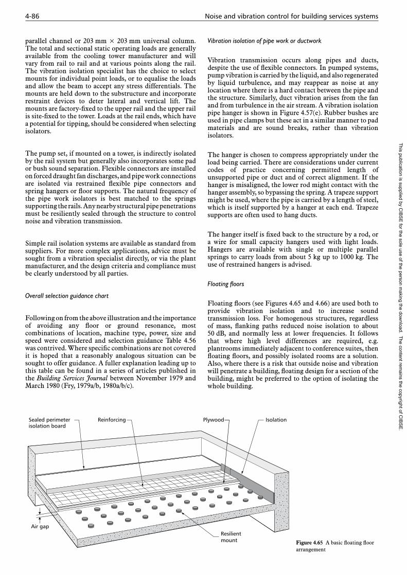
4-86 Noise and vibration control for building services systems
parallel channel or 203 mm × 203 mm universal column. The total and sectional static operating loads are generally available from the cooling tower manufacturer and will vary from rail to rail and at various points along the rail. The vibration isolation specialist has the choice to select mounts for individual point loads, or to equalise the loads and allow the beam to accept any stress differentials. The mounts are held down to the substructure and incorporate restraint devices to deter lateral and vertical lift. The mounts are factory-fixed to the upper rail and the upper rail is site-fixed to the tower. Loads at the rail ends, which have a potential for tipping, should be considered when selecting isolators.
The pump set, if mounted on a tower, is indirectly isolated by the rail system but generally also incorporates some pad or bush sound separation. Flexible connectors are installed on forced draught fan discharges, and pipe work connections are isolated via restrained flexible pipe connectors and spring hangers or floor supports. The natural frequency of the pipe work isolators is best matched to the springs supporting the rails. Any nearby structural pipe penetrations must be resiliently sealed through the structure to control noise and vibration transmission.
Simple rail isolation systems are available as standard from suppliers. For more complex applications, advice must be sought from a vibration specialist directly, or via the plant manufacturer, and the design criteria and compliance must be clearly understood by all parties.
Overall selection guidance chart
Following on from the above illustration and the importance of avoiding any floor or ground resonance, most combinations of location, machine type, power, size and speed were considered and selection guidance Table 4.56 was contrived. Where specific combinations are not covered it is hoped that a reasonably analogous situation can be sought to offer guidance. A fuller explanation leading up to this table can be found in a series of articles published in the Building Services Journal between November 1979 and March 1980 (Fry, 1979a/b, 1980a/b/c).
Vibration isolation of pipe work or ductwork
Vibration transmission occurs along pipes and ducts, despite the use of flexible connectors. In pumped systems, pump vibration is carried by the liquid, and also regenerated by liquid turbulence, and may reappear as noise at any location where there is a hard contact between the pipe and the structure. Similarly, duct vibration arises from the fan and from turbulence in the air stream. A vibration isolation pipe hanger is shown in Figure 4.57(e). Rubber bushes are used in pipe clamps but these act in a similar manner to pad materials and are sound breaks, rather than vibration isolators.
The hanger is chosen to compress appropriately under the load being carried. There are considerations under current codes of practice concerning permitted length of unsupported pipe or duct and of correct alignment. If the hanger is misaligned, the lower rod might contact with the hanger assembly, so bypassing the spring. A trapeze support might be used, where the pipe is carried by a length of steel, which is itself supported by a hanger at each end. Trapeze supports are often used to hang ducts.
The hanger itself is fixed back to the structure by a rod, or a wire for small capacity hangers used with light loads. Hangers are available with single or multiple parallel springs to carry loads from about 5 kg up to 1000 kg. The use of restrained hangers is advised.
Floating floors
Floating floors (see Figures 4.65 and 4.66) are used both to provide vibration isolation and to increase sound transmission loss. For homogenous structures, regardless of mass, flanking paths reduced noise isolation to about 50 dB, and normally less at lower frequencies. It follows that where high level differences are required, e.g. plantrooms immediately adjacent to conference suites, then floating floors, and possibly isolated rooms are a solution. Also, where there is a risk that outside noise and vibration will penetrate a building, floating design for a section of the building, might be preferred to the option of isolating the whole building.
ReinforcingSealed perimeterisolation board
Plywood
Resilientmount
Air gap
Isolation
Figure 4.65 A basic floating floor arrangement
This publication is supplied by CIB
SE
for the sole use of the person making the dow
nload. The content remains the copyright of C
IBS
E.
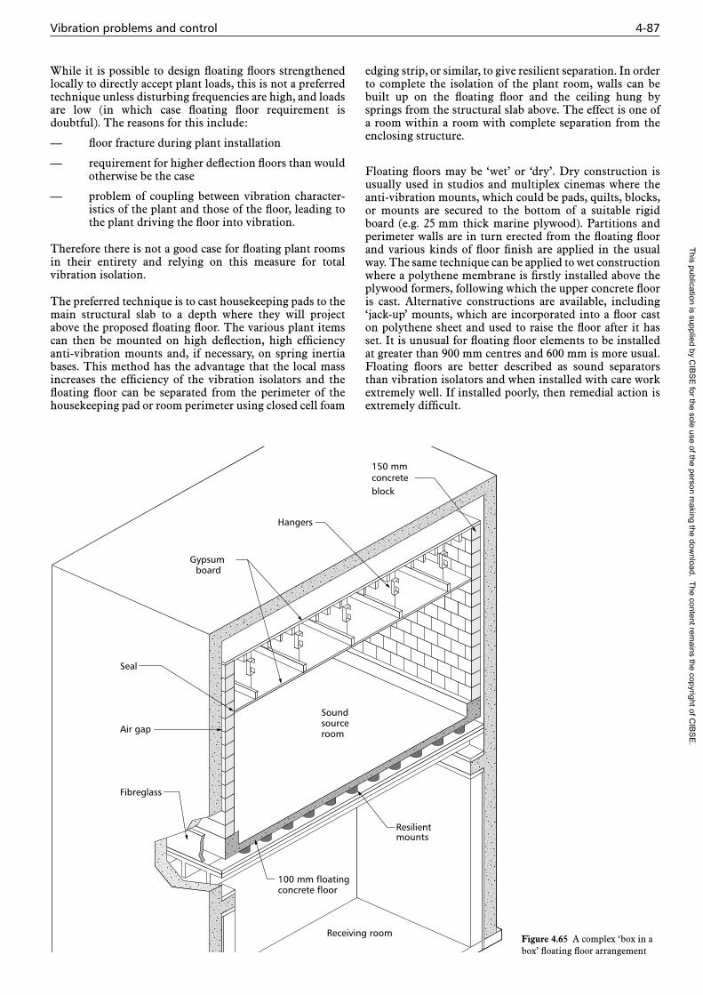
Vibration problems and control 4-87
While it is possible to design floating floors strengthened locally to directly accept plant loads, this is not a preferred technique unless disturbing frequencies are high, and loads are low (in which case floating floor requirement is doubtful). The reasons for this include:
— floor fracture during plant installation
— requirement for higher deflection floors than would otherwise be the case
— problem of coupling between vibration character-istics of the plant and those of the floor, leading to the plant driving the floor into vibration.
Therefore there is not a good case for floating plant rooms in their entirety and relying on this measure for total vibration isolation.
The preferred technique is to cast housekeeping pads to the main structural slab to a depth where they will project above the proposed floating floor. The various plant items can then be mounted on high deflection, high efficiency anti-vibration mounts and, if necessary, on spring inertia bases. This method has the advantage that the local mass increases the efficiency of the vibration isolators and the floating floor can be separated from the perimeter of the housekeeping pad or room perimeter using closed cell foam
edging strip, or similar, to give resilient separation. In order to complete the isolation of the plant room, walls can be built up on the floating floor and the ceiling hung by springs from the structural slab above. The effect is one of a room within a room with complete separation from the enclosing structure.
Floating floors may be ‘wet’ or ‘dry’. Dry construction is usually used in studios and multiplex cinemas where the anti-vibration mounts, which could be pads, quilts, blocks, or mounts are secured to the bottom of a suitable rigid board (e.g. 25 mm thick marine plywood). Partitions and perimeter walls are in turn erected from the floating floor and various kinds of floor finish are applied in the usual way. The same technique can be applied to wet construction where a polythene membrane is firstly installed above the plywood formers, following which the upper concrete floor is cast. Alternative constructions are available, including ‘jack-up’ mounts, which are incorporated into a floor cast on polythene sheet and used to raise the floor after it has set. It is unusual for floating floor elements to be installed at greater than 900 mm centres and 600 mm is more usual. Floating floors are better described as sound separators than vibration isolators and when installed with care work extremely well. If installed poorly, then remedial action is extremely difficult.
Gypsumboard
Soundsourceroom
Resilientmounts
100 mm floatingconcrete floor
Receiving room
Seal
Air gap
Fibreglass
150 mmconcreteblock
Hangers
Figure 4.65 A complex ‘box in a box’ floating floor arrangement
This publication is supplied by CIB
SE
for the sole use of the person making the dow
nload. The content remains the copyright of C
IBS
E.

4-88 Noise and vibration control for building services systems
4.12 Summary
4.12.1 Noise in HVAC systems
Noise in hvac systems is controlled by following the advice given in this section. In particular:
— Choose a quiet fan, which is sized to operate at an efficient point on its characteristic.
— Design for good airflow; aim to minimise turbu-lence and pressure loss, both of which produce noise.
— Include all sources in predictions, e.g. breakout, in addition to duct borne noise.
— Do not forget that building services systems might affect the sound insulation between neighbouring areas.
— Seal all wall penetration with flexible material. This reduces both noise and vibration.
— Choose the location and selection of external plant and air grilles to avoid noise disturbance to nearby properties.
4.12.2 Vibration in HVAC systems
Vibration in hvac systems is controlled by the following the advice given in this section 4.11. In particular:
— Choose a good location for the plant, remote from sensitive areas. This also helps with noise control.
— Ensure that vibration isolation is properly installed with no bridging material across the flexible mountings.
— Ensure that vibration isolators are loaded to give equal deflections and installed to maintain vertical alignment of their springs and other components.
— Remember that misaligned isolators are a source of many problems.
— Check support bolts for integrity and free movement.
— Do not neglect vibration from pipes and ducts; use flexible attachments to the structure.
Further advice is given by Schaffer (1992).
ReferencesASHRAE (2011) HVAC Applications ASHRAE Handbook (Atlanta GA: ASHRAE)
ASHRAE (2013) Fundamentals ASHRAE Handbook (Atlanta GA: ASHRAE)
Beranek LL and Ver IL (eds.) (1992) Noise and Vibration Control Engineering 1st edn. (Chichester: Wiley Interscience)
Beranek LL and Ver IL (eds.) (2005) Noise and Vibration Control Engineering 2nd edn. (Chichester: Wiley Interscience)
BSI (1987) BS 6841: 1987: Guide to measurement and evaluation of human exposure to whole-body mechanical vibration and repeated shock (London: British Standards Institution)
BSI (1994) BS EN 60651: 1994, IEC 60651: 1979: Specification for sound level meters (London: British Standards Institution) [withdrawn]
BSI (1997a) BS EN ISO 11690-1: 1997: Acoustics. Recommended practice for the design of low-noise workplaces containing machinery. Noise control strategies(London: British Standards Institution)
BSI (1997b) BS EN ISO 11690-2: 1997: Acoustics. Recommended practice for the design of low-noise workplaces containing machinery. Noise control measures (London: British Standards Institution)
BSI (1998) BS EN ISO 14163: 1998: Acoustics. Guidelines for noise control by silencers (London: British Standards Institution)
BSI (1999) BS EN ISO 11690-3: 1999: Acoustics. Recommended practice for the design of low-noise workplaces containing machinery. Sound propagation and noise prediction in workrooms (London: British Standards Institution)
BSI (2000a) BS EN 12354-4: 2000: Building acoustics. Estimation of acoustic performance in buildings from the performance of elements. Transmission of indoor sound to the outside (London: British Standards Institution)
BSI (2000b) BS EN 12354-3: 2000: Building acoustics. Estimation of acoustic performance in buildings from the performance of elements. Airborne sound insulation against outdoor sound (London: British Standards Institution)
BSI (2001) BS EN 60804: 2001, IEC 60804: 2001: Integrating-averaging sound level meters (London: British Standards Institution) [withdrawn]
BSI (2003a) BS ISO 226: 2003: Acoustics. Normal equal-loudness-level contours (London: British Standards Institution)
BSI (2003b) BS EN 60942: 2003: Electroacoustics. Sound calibrators (London: British Standards Institution)
BSI (2004a) BS EN 14366: 2004: Laboratory measurement of noise from waste water installations (London: British Standards Institution)
BSI (2005) BS EN ISO 8041: 2005: Human response to vibration. Measuring instrumentation (London: British Standards Institution)
BSI (2007) BS EN ISO 5801: 2008, BS 848-1: 2007: Industrial fans. Performance testing using standardized airways (London: British Standards Institution)
BSI (2008a) BS 6472-1: 2008: Guide to evaluation of human exposure to vibration in buildings. Vibration sources other than blasting (London: British Standards Institution)
BSI (2008b) BS EN 1736: 2008: Refrigerating systems and heat pumps. Flexible pipe elements, vibration isolators, expansion joints and non-metallic tubes. Requirements, design and installation (London: British Standards Institution)
BSI (2009a) BS EN 12354-5: 2009: Building acoustics. Estimation of acoustic performance of building from the performance of elements. Sounds levels due to the service equipment (London: British Standards Institution)
BSI (2009b) BS EN ISO 7235: 2009: Acoustics. Laboratory measurement procedures for ducted silencers and air-terminal units. Insertion loss, flow noise and total pressure loss (London: British Standards Institution)
BSI (2009c) BS EN ISO 5136: 2009: Acoustics. Determination of sound power radiated into a duct by fans and other air-moving devices. In-duct method(London: British Standards Institution)
BSI (2009d) BS 5228-1: 2009 + A1: 2014: Code of practice for noise and vibration control on construction and open sites. Noise (London: British Standards Institution)
BSI (2010a) BS EN ISO 10140-1: 2010 + A2: 2014: Acoustics. Laboratory measurement of sound insulation of building elements. Application rules for specific products (London: British Standards Institution)
BSI (2010b) BS EN ISO 10140-2: 2010: Acoustics. Laboratory measurement of sound insulation of building elements. Measurement of airborne sound insulation (London: British Standards Institution)
BSI (2010d) BS EN ISO 3744: 2010: Acoustics. Determination of sound power levels and sound energy levels of noise sources using sound pressure. Engineering methods for an essentially free field over a reflecting plane (London: British Standards Institution)
This publication is supplied by CIB
SE
for the sole use of the person making the dow
nload. The content remains the copyright of C
IBS
E.

Summary 4-89
BSI (2010c) BS ISO 4866: 2010: Mechanical vibration and shock. Vibration of fixed structures. Guidelines for the measurement of vibrations and evaluation of their effects on structures (London: British Standards Institution)
BSI (2011) BS EN 60534-8-3: 2011: Industrial-process control valves. Noise considerations. Control valve aerodynamic noise prediction method (London: British Standards Institution)
BSI (2013a) BS EN ISO 717-1: 2013: Acoustics. Rating of sound insulation in buildings and of building elements (London: British Standards Institution)
BSI (2013b) BS EN ISO 717-2: 2013: Acoustics. Rating of sound insulation in buildings and of building elements. Impact sound insulation (London: British Standards Institution)
BSI (2013c) BS EN 61672-1: 2013: Electroacoustics. Sound level meters. Specifications (London: British Standards Institution)
BSI (2014a) BS 8233: 2014: Guidance on sound insulation and noise reduction for buildings (London: British Standards Institution)
BSI (2014b) BS EN ISO 16283-1: 2014: Acoustics. Field measurement of sound insulation in buildings and of building elements. Airborne sound insulation (London: British Standards Institution)
BSI (2014c) BS EN 61260-1: 2014: Electroacoustics. Octave-band and fractional-octave-band filters. Specifications (London: British Standards Institution)
BSI (2015) BS EN ISO 16283-2: 2015: Acoustics. Field measurement of sound insulation in buildings and of building elements. Impact sound insulation (London: British Standards Institution)
BSRIA (2012) Understanding acoustic performance data BSRIA BG41 (Bracknell: BSRIA)
CIBSE (2006a) Health issues in building services CIBSE TM40 (London: Chartered Institution of Building Services Engineers)
CIBSE (2006b) Fan application guide CIBSE TM42 (London: Chartered Institution of Building Services Engineers)
CIBSE (2007) Reference data CIBSE Guide C (London: Chartered Institution of Building Services Engineers)
CIBSE (2008) Fan coil units TM43 (London: Chartered Institution of Building Services Engineers)
CIBSE (2015a) Transportation systems in buildings CIBSE Guide D (London: Chartered Institution of Building Services Engineers)
CIBSE (2015b) Environmental design CIBSE Guide A (London: Chartered Institution of Building Services Engineers)
CIBSE (2016a) Heating CIBSE Guide B1 (London: Chartered Institution of Building Services Engineers)
CIBSE (2016b) Ventilation and ductwork CIBSE Guide B2 (London: Chartered Institution of Building Services Engineers)
CIBSE (2016c) Air conditioning and refrigeration CIBSE Guide B3 (London: Chartered Institution of Building Services Engineers)
EC (2002) ‘Directive 2002/44/EC of the European Parliament and of the Council of 25 June 2002 on the minimum health and safety requirements regarding the exposure of workers to the risks arising from physical agents (vibration)’ Official J. of the European Union L177 13–19 (6.7.2002) (available at http://eur-lex.europa.eu/resource.html?uri=cellar:546a09c0-3ad1-4c07-bcd5-9c3dae6b1668.0004.02/DOC_1&format=PDF) (accessed February 2016)
EC (2003) ‘Directive 2003/10/EC of the European Parliament and of the Council of 6 February 2003 on the minimum health and safety requirements regarding the exposure of workers to the risks arising from physical agents (noise)’ Official J. of the European Union L42 38–44 (15.2.2003) (available at http://eur-lex.europa.eu/LexUriServ/LexUriServ.do?uri=OJ:L:2003:042:0038:0044:EN:PDF) (accessed February 2016)
Fry A (1979a) ‘Practical vibration control — Feel the vibration’ J. Chart. Inst. Build. Serv. 1(15) 63–64 (November 1979)
Fry A (1979b) ‘Practical vibration control — From theory to practice’ J. Chart. Inst. Build. Serv. 1(16) 53–54 (December 1979)
Fry A (1980a) ‘Practical vibration control — The six mode problem’ J. Chart. Inst. Build. Serv. 2(1) 48–49 (January 1980)
Fry A (1980b) ‘Practical vibration control — Total engineering’ J. Chart. Inst. Build. Serv. 2(2) 47–48 (February 1980)
Fry A (1980c) ‘Practical vibration control — Into the real world’ J. Chart. Inst. Build. Serv. 2(3) 52–54 (February 1980)
HSE (2005) Controlling noise at work. The Control of Noise at Work Regulations 2005. Guidance on Regulations L108 (Bootle: Health and Safety Executive) (available at http://www.hse.gov.uk/pubns/priced/l108.pdf) (accessed February 2016)
HEVAC (1979) Real Room Acoustic Test Procedure (Reading: HEVAC Association) (available at https://www.feta.co.uk/uploaded_images/files/HEVAC/Air_distribution/Real%20Room%20Acoustic%20Test%20procedure.pdf) (accessed February 2016)
ISO (1998a) ISO 140-4: 1998: Acoustic. Measurement of sound insulation in buildings and of building elements. Part 4: Field measurements of airborne sound insulation between rooms (Geneva: International Organization for Standardization) [withdrawn; replaced by BS EN ISO 16283-1 (BSI, 2014)]
ISO (1998b) ISO 140-7: 1998: Acoustics. Measurement of sound insulation in buildings and of building elements. Part 7: Field measurements of impact sound insulation of floors (Geneva: International Organization for Standardization) [withdrawn; replaced by BS EN ISO 16283-2 (BSI, 2015)]
ISO (2007) ISO 1996-2: 2007 Ed 2: Acoustics. Description, assessment and measurement of environmental noise. Determination of environmental noise levels (Geneva, Switzerand: International Standards Organization)
ISO (2008) ISO/IEC GUIDE 98-3: 2008 Ed 1: Uncertainty of measurement. Guide to the expression of uncertainty in measurement (Geneva, Switzerand: International Standards Organization)
NBS (2015) Resistance to the passage of sound Building Regulations Approved document E (2003 edition incorporating 2004, 2010, 2013 and 2015 amendments) (Newcastle upon Tyne: NBS) (available at http://www.planningportal.gov.uk/buildingregulations/approveddocuments/parte/approved) (accessed February 2016)
NEBB (1994) Sound and vibration design and analysis (Gaithersburg MD: National Environmental Balancing Bureau)
Schaffer M (1992) A practical guide to noise and vibration control for hvac systems (Atlanta GA: American Society of Heating, Refrigerating and Air-Conditioning Engineers)
Sharland IJ (1972) Fläkt Woods Practical Guide to Noise Control (Colchester: Woods of Colchester)
Shultz TJ (1985) ‘Relationship between sound power level and sound pressure level in dwellings and offices’ RP-339 ASHRAE Trans. 91(1A)
Sound Research Laboratories (1987) Noise Control in Building Services (Oxford: Pergamon Press)
Tauby JR and Lloyd R (2012) A Practical Guide to Seismic Restraint (Atlanta GA: ASHRAE)
TSO (2005) The Control of Noise at Work Regulations 2005 Statutory Instruments No. 1643 2005 (London: The Stationery Office (TSO)) (available at http://www.legislation.gov.uk/uksi/2005/1643) (accessed February 2016)
TSO (2010) The Building Regulations 2010 Statutory Instruments 2010 No. 2214 (London: The Stationery Office (TSO)) (available at http://www.legislation.gov.uk/uksi/2010/2214) (accessed February 2016)
Ver IL (1984) ‘Prediction of sound transmission through duct walls: Breakout and pickup’ KC-2851 (RP-319) ASHRAE Trans. 90(2a) (Atlanta, GA: ASHRAE)
Waddington DC and Oldham DJ (1999) ‘Generalized flow noise prediction curves for air duct elements’ J. Sound and Vibration 222(1) 163–169 (available at https://www.researchgate.net/publication/234184274_Generalized_Flow_Noise_Prediction_Curves_for_Air_Duct_Elements) (accessed February 2016)
This publication is supplied by CIB
SE
for the sole use of the person making the dow
nload. The content remains the copyright of C
IBS
E.

4-90 Appendices
Appendix 4.A1: Explanation of some basic acoustic concepts
4.A1.1 The nature of sound and noise
Sound is produced by very small but rapid pressure fluctuations in the air. Noise is often simply defined as ‘unwanted’ sound and thus the terminology described below applies equally to both terms.
The sound pressure is the instantaneous change in atmospheric pressure caused by the sound wave. In the simplest of all possible sounds, called a pure tone, the variation in sound pressure with time is sinusoidal, and the frequency of the sound is the number of cycles of pressure variations per second, measured in hertz (Hz).
The frequency of the fluctuations may be between 20 times a second (20 Hz), or lower for some fan instabilities, and up to 20 000 times a second for audible noise. However, for hvac, we are not normally concerned with frequencies above 4000 Hz or, occasionally, 8000 Hz.
Sound pressure is measured in pascals (Pa), (where 1 Pa = 1 N/m2). The human hearing range extends from about 20 × 10–6 Pa (the threshold of hearing) to about 100 Pa, which is about one thousandth of steady atmospheric pressure.
4.A1.2 Broad band noise and tonality
Most sounds contain a mixture of a wide range of frequencies and are called broad band sounds. Examples are the sound (or noise) from vacuum cleaner, washing machines, motor vehicles and fans. The relative amounts of sound energy at different frequencies may be determined by carrying out a frequency analysis, according to which the sound pressure levels are measured in a range of frequency bands. The most common methods involve either octave or ⅓-octave bands (see Appendix 4.A6).
Sometimes an otherwise broad band noise may also contain pure tone components, often described by terms such as hum, squeak, whine, whistle.
Such tonal components are usually accepted as being more annoying and therefore noise containing tones is often assessed more severely than the corresponding broad band noise without tones. It is therefore important to have objective methods of determining the presence of tonal components in a noise, rather than relying on subjective assessment.
The presence of tonal components in a noise may sometimes be reflected in the shape of the noise spectrum whereby one of the octave or ⅓-octave band levels (containing the tonal frequency) stands out as being several decibels higher than its immediate neighbours. More accurate methods of objectively determining tonality are given in ISO 1996-2 (ISO, 2007) (see Appendix 4.A4.7).
4.A1.3 Sound frequency, wavelength and velocity
In addition to frequency, the quantities that define a sound wave include:
— wavelength, λ
— velocity, c = 345 m·s–1 (approximately, depending on temperature).
Wavelength, frequency and velocity are related by the following equation:
c = λ f (4.A1.1)
where c is the velocity (m·s–1), λ is the wavelength (m) and f is the frequency (Hz).
Thus frequency can be related to wavelength, see Table 4.A1.1.
It is useful to develop an appreciation of frequencies and related wavelengths, since this helps an understanding of the operation of noise control. Low frequencies (63, 125 and 250 Hz have long wavelengths and high frequencies (1000, 2000 and 4000 Hz) have much shorter wavelengths — the range extends from the size of a matchbox to the length of a bus).
The significance of frequency and wavelength
Most noise, including that from building services, does not consist of a single frequency, but contains a mix of all frequencies, called broad band noise. The frequency content of a noise is important because human hearing is frequency sensitive and the performance of sound insulating and absorbing materials used to reduce noise levels also depend on frequency, in such a way that it is usually easier to reduce high frequency noise than that at low frequencies. The frequency of the sound also determines its wavelength.
Wavelength determines the directionality of sound sources of microphones and of human hearing and the insertion loss of screens and barriers.
The frequency content of a sound is determined by the sound source. The sound speed is determined by the medium and varies with temperature. The frequency and
Table 4.A1.1 Relation between frequency and wavelength of sound
Frequency / Hz Wavelength / λ (m)
63 5.5
125 2.8
250 1.4
500 0.69
1000 0.35
2000 0.17
4000 0.86
This publication is supplied by CIB
SE
for the sole use of the person making the dow
nload. The content remains the copyright of C
IBS
E.

Explanation of some basic acoustic concepts 4-91
sound speed then determine the wavelength. Therefore when, for example, a sound generated by a fan is transmitted into water or into the structure of building and later to be transmitted back into airborne sound at a receiver location, the frequency of the sound will be the same the wavelenght will have changed depending on the medium.
4.A1.4 Sound power, intensity and pressure
Sound sources such as fans loudspeakers and human voices radiate sound energy into the surrounding environment. The defining characteristic of a sound source is the rate at which it radiates sound energy in watts (W). The sound power of a human voice when shouting may be about 1 mW, that of a large fan in a hvac system about 1 W and the banks of loudspeakers at a pop concert hundreds of watts.
The sound energy radiated by the sources spreads out as it travels into the surrounding environment and its effect at any point may be described either as a sound pressure or as a sound intensity.
Sound pressure is the force per unit of area produced by the sound and has units of pascals (Pa) (i.e. N·m–2). The sound pressure fluctuates above and below atmospheric pressure by a small amount and a time average may be zero. The sound pressure is therefore quantified by the square root of the square of the fluctuations, giving the root mean square (Rms) value. (Squaring the pressure fluctuations makes all values positive.)
The sound intensity is a measure of the rate of flow of sound energy in watts per square metre (W·m–2). This is analogous to the amount of illumination produced by a light source.
The sound intensity and sound pressure are related; the intensity is proportional to the square of the sound pressure, so that if the sound pressure is doubled the sound intensity increases by a factor of four. This relationship is important in determining how sound pressures may be described in decibels, as shown later.
In summary: the sound power is a characteristic of the sound source, expressed in watts (W). It is a fundamental quantity associated with the source alone. Sound intensity and sound pressure are quantities which describe the magnitude of the sound at various positions in the environment surrounding the source, and they depend on the transmission path from source to receiver as well as on the sound power of the source.
All three of these quantities are more usually measured in decibels, as sound power levels, sound pressure levels and sound intensity levels. Noise levels are simply measured as sound pressure levels.
4.A1.5 The decibel scale: sound power level, sound intensity level and sound pressure level
The decibel scale is a logarithmic scale used for comparing ratios of powers, or quantities related to powers.
The logarithm (or ‘log’, ‘lg’) of a number is the power or index that a certain base value (in this case it is 10) must be raised in order to give the number in question.
For example, 10 may be written as 101 so that:
lg10 10 = 1 (4.A1.2)
100 may be written 10 × 10 = 102 so that:
lg10 100 = 2 (4.A1.3)
1000 may be written as 10 × 10 × 10 = 103
so that:
lg10 1000 = 3 (4.A1.4)
(Note that the reverse process, the antilogarithm (or antilog) restores the original number, so that whereas log10 1000 = 3; antilg10 3 = 103 =1000.)
Two sound powers W1 and W2 may be compared on a decibel scale by taking the log of the ratio and then multiplying by 10, so that the difference in decibels between the two is:
N dB = 10 × lg10 ( W1 / W2 ) (4.A1.5)
On a decibel scale source 1 has a sound power level that is N dB higher than source 2.
Note that the multiplying factor of 10 (the ‘deci’ in decibels) is simply used to produce a convenient range of values for the audible sound range; the scale would otherwise be in bels.
Table 4.A1.2 gives the difference in decibels corresponding to various power ratios.
A logarithmic scale is one in which equal percentage changes in a quantity are denoted by equal increments of the scale. From the above table for example each doubling of power results in an increase of 3 dB and each tenfold increase results in a change of 10 dB. The table also illustrates a useful feature of the decibel scale (arising from
Table 4.A1.2 Differences in decibels at various power ratios
Power ratio,
W1/W2
Difference
/ dB
1 0
2 3
3 5
4 6
5 7
8 9
10 10
20 13
40 16
100 20
1000 30
10 000 40
100 000 50
1 000 000 60
This publication is supplied by CIB
SE
for the sole use of the person making the dow
nload. The content remains the copyright of C
IBS
E.

4-92 Appendices
its logarithmic basis) that calculations which would involve multiplications or divisions when operating in watts are more conveniently replaced by additions and subtractions in decibels. Thus the decibel equivalents of ratios obtained by multiplying values in the ratio column may be obtained by adding the corresponding values from the decibel column. Thus a ratio of 40 (= 4 × 10) corresponds to a dB change of 16 dB (= 6 +10). In this way other values not in the table may easily be derived; so that, for example a power ratio of 300 (= 3 × 100) corresponds to a change in decibel level of 25 dB (= 5 + 20).
The decibel scale, because it is logarithmic, compresses wide range of values into a smaller range. For example in the above table a ratio of 1000 000 becomes a 60 dB change. This approach is advantageous for handling sound pressures, where the ratio of the highest to the lowest sound likely to be encountered, is as high as 1000 000:1.
Sound power level
Although the above equation and Table 4.A1.2 are useful for comparing sound powers relative to each other it is also useful to specify absolute levels. For this purpose a base or reference value, W0 has been defined:
W0 = 1 × 10–12 W (4.A1.6)
Using this base value an absolute value of sound power level LW is defined:
LW = 10 lg (W / W0) in dB re. 10–12 W (4.A1.7)
From this definition it can be seen that for a sound power of W = 1 watt, LW = 120 dB.
If the sound power is doubled (and for every subsequent further doubling) it increases by 3 dB. If the sound power increases tenfold (and for every subsequent further tenfold increase) the sound power level increases by 10 dB.
Sound intensity level
A sound intensity level LI may be similarly be defined by specifying a reference value of I0 = 1 × 10–12 W/m2 which, approximately corresponds to the average threshold of human hearing:
LI = 10 lg ( I / I0 ) in dB re. 10–12 W/m2 (4.A1.8)
From this definition it can be seen that for a sound intensity of I = 1 W/m2, LI = 120 dB.
If the sound intensity increases is doubled (and for every subsequent further doubling) the sound intensity level increases by 3 dB. If the sound intensity increases tenfold (and for every subsequent further tenfold increase) the sound intensity level increases by 10 dB.
Sound pressure level
The reference value for sound pressure, p0, is defined as 2 × 10⁻⁵ Pa which, as for I0 approximately corresponds to the average threshold of human hearing. In order to define a sound pressure level it is necessary to invoke the relationship that sound intensity is proportional to sound pressure squared, so that in the above definition the ration (I / I0 ) may be replace by ( p / p0 )
2. Using a well-known
property of logarithms that squaring a number corresponds to doubling its logarithm then:
10 lg ( p / p0) 2 = 20 lg ( p / p0 ) (4.A1.9)
On this basis:
Lp = 10 lg (p / p0)2 = 20 lg (p / p0) re. 2 × 10⁻⁵ Pa
(4.A1.10)
From this definition it can be seen that for a sound pressure of p = 1 Pa, Lp = 94 dB.
If the sound pressure is doubled (and for every subsequent further doubling) the sound pressure level increases by 6 dB. If the sound pressure increases tenfold (and for every subsequent further tenfold increase) the sound intensity level increases by 20 dB.
When the word ‘level’ is used in connection with sound or noise, decibel levels are implied, denoted by LX, where the subscript ‘X’ is the symbol for the appropriate quantity. Sound pressure level is denoted as Lp but also sometimes as spl. Sound power level is denoted as LW but also sometimes as swl. Sometimes ambiguity can arise as to whether a decibel level is a sound pressure level or a sound power level. Such ambiguities may be removed if the reference quantities are quoted, for example 85 dB re. 2 × 10⁻⁵ Pa clearly indicates a sound pressure level, whereas 105 dB re. 10–12 W clearly denotes that it is a sound power level that is being referred to. Where, as is usually the case, the reference quantities are omitted the context should indicate whether it is a sound pressure or sound power level.
Although meters are available which will measure sound intensity, it is much more usual to measure sound pressure levels, using a sound level meter (see Appendix 4.A4). The reason for this is that human hearing senses sound pressure fluctuations at the ear drum and microphones, in sound level meters operate in a rather similar way whereby a diaphragm which, deflecting under the fluctuating force of the sound wave, converts its deflection to an electrical signal. Since pressure = force/area, it is the sound pressure which applies a force to the diaphragm.
The reference values for pressure and intensity have been chosen to be close to normal thresholds of hearing, so that the threshold on the decibel scale is approximately 0 dB. An advantage of these choices is that they are related in such a way that the decibel values of sound pressure level and sound intensity level are the same for the same sound, to within about 0.5 dB.
4.A1.6 Sound power levels of sources and sound pressure levels in rooms
An important way in which the acoustic designer may limit noise from building services is to specify maximum noise emission levels from items of plant.
Sound emission from a sound source may be specified in two ways: either as a sound power level or as a sound pressure level at a specified distance from the source. The first method is usually thought preferable because the sound power level relates to the source alone, independent
This publication is supplied by CIB
SE
for the sole use of the person making the dow
nload. The content remains the copyright of C
IBS
E.

Explanation of some basic acoustic concepts 4-93
of the environment in which it is situated, whereas for the second method the test environment must also be considered. However laboratory sound power level test data must be available because sound power level is not otherwise easy to determine.
In either case the data is needed in octave bands rather than just as dBA, dBC or dBZ levels.
4.A1.7 Variation of sound pressure and sound pressure level with distance from the source
If the source is located outdoors, well away from sound reflecting surfaces, then the sound pressure level decreases as the distance from the source increases, according to a simple model of sound propagation at a rate of 6 dB per doubling of distance (which corresponds to the inverse square law expressed in decibels). When the source is located in an enclosed space the sound level will at first decrease with distance as for the outdoor case, until it eventually reaches an approximately constant level, when the reflections from the room surfaces have greater influence than the sound radiated directly from the source. This constant level depends on the size of the room and the amount of sound absorption it contains.
Sound pressure level in rooms may be predicted from the sound power level of sound sources, but predictions may be based on simplistic models of sound propagation in rooms, and may be of limited accuracy, and should only be used by those with experience who are aware of their limitations. The prediction of sound pressure levels in rooms is discussed in more detail in section 4.7.
The important issues for the acoustic designer arising from the way sound behaves in rooms are; firstly to be aware that the same item of plant, i.e. with the same sound power level, may produce different sound pressure levels in different spaces (dependent on distance from source, volume and sound absorption of the room); and, secondly, that when specifying noise limits it might be necessary to specify positions in the room where these should apply. These positions could, for example, be typical of where people might be, or might represent either worst case or best case situations, or be at specified positions within the room, e.g. at a certain distance from the nearest wall.
If the source is small compared with the wavelength, it approximates to an idealised point source which radiates spherical waves equally in all directions, provided that there are no nearby sound reflecting surfaces. The inverse square law of radiation then applies, similar to sources of light, and at a distance r the sound energy from the source will be spread over a sphere of area 4 π r2 . The intensity is:
I = W / (4 π r2) (4.A1.11)
where I is the intensity (W·m–2), W is the sound power (W) and r is the distance from the source (m).
By substituting numerical values, and converting to logarithms, the intensity level can be expressed in decibels as:
LI = LW – (20 lg r) – 11 (4.A1.12)
where LI is the sound intensity level (dB), LW the sound power level (dB) and r is the distance from the source (m).
But, as the decibel sound pressure levels and sound intensity levels are numerically the same, this can immediately be written in the more familiar pressure terms as:
Lp = LW – (20 lg r) – 11 (4.A1.13)
If the sound is constrained into a hemisphere by reflecting surfaces, the surface area for radiation changes from (4 π r2) to (2 π r2) and the sound pressure level becomes:
Lp = LW – (20 lg r) – 8 (4.A1.14)
The (20 lg r) term for free propagation, either spherical or hemispherical, means that if distance r is doubled or halved the pressure level change is 6 dB (i.e. because 20 lg 2 = 6).
Thus a sound power level of 100 dB will produce a sound pressure level of 89 dB at a distance of 1 m from the source, 83 dB at a distance of 2 m, 77 dB at 4 m and so on, and these levels would all be increased by 3 dB if the source was located above a sound reflecting plane.
4.A1.8 Directionality: intrinsic and positional
Out in the open well away from any sound reflecting surfaces (so called free field conditions) a noise source such as a machine or a loudspeaker, or a human voice may send out more sound in one direction than another. This is the intrinsic directionality or directivity of the sound source and is usually dependent on frequency, most sources become more directional at higher frequencies than they are at lower frequencies.
If such a source is now located close to a sound reflecting surface, for example hard ground, or a wall, outdoors, or a wall floor or ceiling indoors, then it will be constrained to radiate sound in certain directions but not in others, and thus in effect acquires a directionality or directivity as a result of its position.
Thus, for example, a source which is omnidirectional out in the open, i.e. which radiates sound equally in all directions under so called free field conditions, will be constrained to radiate sound upwards only when placed on a hard sound reflecting surfaces.
The directionality of the source, whether intrinsic or positional, may be described by comparing its sound output in any particular direction with that which would be emitted in that same direction by an omnidirectional source with the same total power.
Two such measures are used: directivity factor and directivity index.
— Directivity factor (Q): expresses, as a ratio, the amount of sound energy radiated in a particular direction, as compared to the amount radiated by an omnidirectional source of the same total sound power in the same direction. Thus a Q of 2 in a given direction means that twice as much power is being radiated in that direction if the sound had been radiated equally in all directions, and a Q of 0.5 means that only half as much sound energy is
This publication is supplied by CIB
SE
for the sole use of the person making the dow
nload. The content remains the copyright of C
IBS
E.
4-94 Appendices
radiated in the specified direction, as on average, in all directions.
— Directivity index (D): expresses, in decibels, the same comparison, between sound energy radiated in a particular direction and the average over all directions. Thus for example a directivity index of + 3 dB means that twice as much sound energy is radiated in that particular direction than on average over all directions, and correspondingly a value of D = –3 dB means that only half as much sound energy is radiated in the specified direction, as on average, in all directions.
The two measures of directionality are simply related:
D = 10 lg Q (4.A1.15)
4.A1.9 Sound power levels and sound pressure levels in a duct
If the sound is constrained in a duct it does not spread out and so does not reduce in intensity as the distance increases. Therefore the intensity (W·m–2) in a duct of constant cross-section will remain constant in the absence of losses. However, losses always occur by breakout, energy transfer to duct wall vibration, absorption etc. The internal noise level in a duct section near to the fan is typically 90–100 dB and proper design reduces it to around 35 dB in the room. By using the equations for sound intensity and sound power, it follows that a sound pressure level/sound intensity level of 96 dB in a duct of 0.5 m2 cross sectional area, equates to the sound power into the duct of 2 × 10⁻³ W (i.e. 2 milliwatts). A general relation for sound intensity, area and sound power is:
LW = LI + 10 lg S (4.A1.16)
where S is the cross sectional area of the duct (m2).
Then for the example above, where the area is 0.5 m2, sound power in the duct is:
LW = 96 + 10 lg 0.5 = 93 dB
Working backwards and converting sound power level (dB) to sound power (W) using equation 4.A1.7:
W = 10–12 antilg 9.3 = 2 × 10⁻³ W (4.A1.17)
However, as the decibel levels for pressure and intensity are equal, equation 4.A1.16 can also be written as:
LW = Lp + 10 lg S (4.A1.18)
The sound power level is not numerically the same as the sound pressure or intensity level (except for ducts having a cross-sectional area of 1 m2, since 10 lg S is then zero). Sound pressure and sound intensity levels are affected by the sound propagation path between source and receiver.
When calculating duct system noise, the fundamental quantity is the sound power entering or leaving a duct element. This continues up to the duct termination, which acts as a source of power into the room, from which the room sound level is predicted, see section 4.5.7.
Equation 4.A1.16 is also useful for estimating the level at a distance from an extended source, such as boiler house louvres or an opening in a wall. If the sound pressure level averaged over the extended source is known, combining this with the area gives the sound power level, which can then be used with equation 4.A1.14 to determine the level at a distance. However, large sources are directional, so that equation 4.A1.14 will underestimate at higher frequencies in directions to the front of the source.
4.A1.10 Decibel arithmetic: combining, subtracting and averaging sound pressure levels
Combining decibel levels enables estimates to be made of the total level which will occur when the known sound levels from different sources are combined; for example when estimating the total sound pressure level which will occur in a plant room when various combinations of plant are switched on. Conversely, subtracting levels allows estimates to be made of the effect on the total level of removing or eliminating one or more of these component sounds. Decibel subtraction is also widely used to make a correction for the presence of background noise on the measurement of sound pressure level from items of plant. Averaging of sound pressure levels becomes necessary when several measurements are taken, at several different positions in a room for example, in order to achieve the most accurate and reliable result.
As decibels are logarithmic ratios, they do not add arithmetically. It is necessary to convert back to the original physical units, add, subtract or average values of sound intensity or (pressure2) and then re-convert the result back to decibels. This means first converting the decibel levels, L, using antilogs (i.e. 10NL/10), summing (or subtracting, or averaging as appropriate), and then converting back into decibels by taking 10 times the logarithm of the result.
Example 4.A1.1
(a) Add 55 dB and 57 dB sound pressure levels
From equation 5.A1.3:
55 dB = 20 lg ( p1/p0 ) = 10 lg ( p1/p0 )2
Then:
( p1/p0 )2 = antilg 5.5 = 105.5
Similarly:
(p2/p0 )2 = antilg 5.7 = 105.7
Since (unlike decibel levels) values of p2 may be added arithmetically, the sum, or total sound pressure, pT, is given by:
(pT /p0) 2 = (p1/p0)
2 + (p2/p0) 2
Therefore:
(pT /p0) 2 = 10 5.5 + 10 5.7
= 316 228 + 501187 = 817 415
This publication is supplied by CIB
SE
for the sole use of the person making the dow
nload. The content remains the copyright of C
IBS
E.

Explanation of some basic acoustic concepts 4-95
Hence, the sum or total of the two levels, LT in dB, is:
LT = 10 lg (817 415) = 59.1 dB
which would normally be rounded to 59 dB.
These steps may be combined into the following formula, which may be extended to the combination of any number of dB levels (L1, L2, L3 ... LN):
LTotal = 10 lg [10L1/10 + 10L2/10 + … + 10LN/10]
In the above example:
LTotal = 10 lg [105.5 + 105.7] = 59.1 dB
This formula can easily be implemented using a calculator or computer spreadsheet.
(b) Subtract 60 dB from 61 dB
Proceeding as above:
10 6.1 – 10 6.0 = 1 258 925 – 1 000 000 = 258 925
Hence:
10 lg (258 925) = 54 dB
This shows that if a noise of level 60 dB has one of level 54 dB added to it, the resulting level is 61 dB.
In the above examples it was necessary to work back to the original quantities, (e.g. sound pressure), which is a measure of the energy in the sound wave, add or subtract them, and then work forward to determine the total decibel level.
Decibel subtraction may also be carried out using the following formula, which gives the resulting level LR when level L2 is subtracted from the higher level L1:
LR = 10 lg (10 L1/10 – 10 L2/10)
The logarithmic (or sound energy related) average of several sound pressure levels: L1, L2, L3 … LN may be found using the formula below:
LAVERAGE = 10 lg [ (10 L1/10 + 10 L2/10 + ...
.... + 10 LN/10) / N]
To simplify addition and subtraction Figure 4.A1.1 can be used. For addition, the scales are used as shown. For subtraction, enter the difference between the two levels on the upper scale. The amount to be subtracted from the smaller decibel level is given on the bottom scale.
Example 4.A1.2
The calculations performed in Example 4.A1.1 are carried out using Figure 4.A1.1, as follows.
(a) Add 55 dB and 57 dB sound pressure levels:
— bottom scale: difference between levels to be added is (57 – 55) = 2 dB
— top scale: corresponding value to be added to the higher level is 2.1 dB
— sum is (57 + 2.1) = 59.1 dB.
(b) Subtract 60 dB from 61 dB:
— top scale: difference between levels to be subtracted is (61 – 60) = 1 dB
— bottom scale: corresponding value to be subtracted from the smaller level is 6 dB
— difference is (60 – 6) = 54 dB.
As an alternative to the chart method Table 4.A1.3 may be used for combining levels. Decibel levels may be combined in pairs. A correction is added to the higher of the two levels depending upon the difference between the two levels. The use of the table is accurate to the nearest decibel. In the above example (to combine levels of 55 dB and 57 dB) the difference of 2 dB leads to the addition of 2 dB to the higher level resulting in 59 dB, to the nearest dB. Table 4.A1.4 may be used for subtracting decibel levels.
Table 4.A1.3 Combining decibels (accurate to the nearest dB)
Difference between levels
Add to the higher level
0 3
1 3
2 2
3 2
4 1
5 1
6 1
7 1
8 1
9 1
10 0 (< 0.5)
Table 4.A1.4 Subtracting decibel levels
Difference between levels
Subtract from lower level
1 6
2 4
3 3
4 2
5 1.5
7 1
2·53
0
2 11·5 0·8
Difference between two levels, in decibels
Decibels to be added to higher level
0·6 0·4 0·2
5 10 15
Figure 4.A1.1 Line chart for addition of sound pressure levels
This publication is supplied by CIB
SE
for the sole use of the person making the dow
nload. The content remains the copyright of C
IBS
E.

4-96 Appendices
4.A1.11 Unweighted and A-weighted sound power levels
Many sound sources produce more sound power at lower frequencies than at lower frequencies and in these cases the A-weighted sound power levels will be very different from the unweighted values as shown by the example below, in which the sound power levels are specified in octave bands.
These sound power levels are used to predict sound pressure levels at various positions around the sound source. It is very important to establish whether a manufac turer’s declared sound power levels are unweighted or not. Usually a good indication may be obtained from a visual inspection of the spectral values, but where there is any doubt or ambiguity clarification should be obtained from the manufacturer or supplier.
A similar method may be used to convert predicted octave band sound pressure levels to dBA (or dBC if the C-weighting values replace A-weighting in Table 4.A1.5) levels during the design stages, but this will rarely be necessary for measured sound pressure levels since sound level meters are fitted with A- and C-frequency weighting filters (see Appendix 4.A4).
Table 4.A1.5 Unweighted and A-weighted sound power levels
Octave band centre frequency
/ Hz
Unweighted sound power
level / dB
A-weighting / dB*
A-weighted octave band sound power
level / dB
31.5 100 –39 61
63 97 –26 71
125 94 –16 78
250 99 –9 90
500 93 –3 90
1000 85 0 85
2000 74 1 75
4000 68 1 69
8000 60 –1 59
Overall unweighted sound power level (obtained by combining the levels in column 2): 104 dB
Overall A-weighted sound power level (obtained by combining the levels in column 4): 94 dBA
* rounded to the nearest dB for simplicity
Appendix 4.A2: Regeneration of noise by duct components and terminations
4.A2.1 Bends, takeoffs, transitions
This method, which is based on work at Liverpool University (Waddington and Oldham, 1999), is applicable to in-duct components such as bends, transition pieces and take-offs, but is not appli cable to termination devices. It is based upon a theoretical model for rectangular ductwork but is also applicable to circular section ductwork.
For a particular element, the required information is pressure loss factor (ζ ) obtained from section 4 of CIBSE Guide C (2007) or other data source, duct cross sectional dimensions and air velocity. It is necessary to determine an approximate value of the clear area ratio (σ ) and a characteristic dimension (d).
These can be estimated from pressure loss factor as follows.
The clear area ratio is given by:
σ ζ
ζ= −
−
1 2 1
1
/
(4.A2.1)
where σ is the clear air ratio and ζ is the pressure loss factor.
The characteristic dimension is given by:
d = b (1 – σ) (4.A2.2)
where d is the characteristic dimension (m) and b is the duct dimension in the direction of flow constriction (m) (see Figure 4.A2.1).
Figure 4.A2.1 illustrates how the flow of air is constrained in one direction when it encounters a mitred bend. Similar effects are observed for other in-duct elements.
b
Stream lines
Figure 4.A2.1 Constriction in a duct
1·60 0·2 0·4 0·6 0·8 1·0 1·2 1·4Pressure loss factor ( )ζ
0·9
0·8
0·7
0·6
0·5
0·4
Cle
ar a
ir r
atio
(
)σ
Figure 4.A2.2 Determination of clear air ratio from pressure loss factor
This publication is supplied by CIB
SE
for the sole use of the person making the dow
nload. The content remains the copyright of C
IBS
E.

Regeneration of noise by duct components and terminations 4-97
A graph giving σ in terms of ζ is shown in Figure 4.A2.2. There are different expressions for noise regeneration below and above the duct ‘cut-on’ frequency, which is the frequency above which complex acoustic modes are propagated in the duct; propagation is as a plane wave below the cut-on frequency.
The cut-on frequency is given by:
c fc = —– (4.A2.3)
2 l
where fc is the cut-on frequency (Hz), c is the velocity of sound (m·s–1) and l is the longest duct cross sectional dimension (m).
Where the required octave band frequency (fo) is below cut-on (i.e. fc > fo ), the sound power generated by the fitting is:
LW = –37 + 20 lg (K (Sr)) + 20 lg ζ
+ 10 lg A + 40 lg u (4.A2.4)
where LW is the sound power level (dB), K (Sr) is an experimentally determined factor related to the Strouhal number, ζ is the pressure loss factor, A is the cross sectional area of the duct and u is the air velocity in the duct (m·s–1).
For fc < fo, where the required octave band frequency (fo) is above the cut-on frequency:
LW = –84 + 20 lg (K (Sr)) + 20 lg (Sr)
+ 10 lg ζ – 40 lg σ + 10 lg A + 60 lg u
(4.A2.5)
where (Sr) is the Strouhal number.
The term 20 lg (K(Sr)) is determined as follows. K(Sr) is an experimentally determined factor, see Figure 4.A2.3, where the vertical axis on the curve is 20 lg (K(Sr)) and the horizontal axis is the Strouhal number Sr.
So, a value for 20 lg (K (Sr)) may be obtained if the Strouhal number is known. (Note: Figure 4.A2.3 is based on data for a variety of air velocities in two different duct sizes and has an accuracy of around ±2 dB. Similar curves have been obtained for other elements.)
The Strouhal number is given by the equation:
Sr = f d / vc (4.A2.6)
where Sr is the Strouhal number, f is the frequency, d is the characteristic dimension (m) (see equation 4.A2.6) and vc is the constriction velocity (m·s–1).
The constriction velocity is given by:
vc = u /σ (4.A2.7)
where u is the air velocity in the duct (m·s–1) and is σ the clear air ratio (see equation 4.A2.5).
The procedure for determining the regenerated noise level for a given octave band frequency is as follows:
— calculate Sr from d and σ (both functions of ζ) and air velocity u
— read off appropriate value of 20 lg (K (Sr)) from Figure 4.A2.3
— insert values in the above equations depending on whether the octave band frequency (fo) is below or above duct higher mode cut-on (fc = c / 2 l) (equation 4.A2.3).
Other terms in the equations are physical constants or duct dimensions.
Thus, from knowledge of pressure loss coefficient, duct dimensions and air velocity one can calculate the sound power level for any chosen octave band centre frequency.
Example 4.A2.1
A duct element of 600 mm by 400 mm, where the 400 mm dimension is in the direction of the constricted flow, has pressure loss factor (ζ) of 1.25, and a clear air ratio (σ) of 0.47.
Given the duct dimension in the direction of constricted flow as 400 mm, from equation 4.A2.2 the characteristic dimension is:
d = 0.4 (1 – 0.47) = 0.21 m
For an air velocity (u) of 15 m·s–1, the constriction velocity is obtained from equation 4.A2.7:
vc = 15 / 0.47 = 31.9 m·s–1
From equation 4.A2.3, the duct cut-on frequency for higher modes is:
fc = 345 / (2 × 0.6) = 288 Hz
Then, from equation 4.A2.6, for fo = 125 Hz, the Strouhal number is:
Sr = 125 × 0.21 / 31.9 = 0.82
Estimating from Figure 4.A2.3, a Strouhal number of 0.82 gives 20 lg (K (St)) = 75. Then, as the frequency is below cut-on, equation 5.A2.8 applies, i.e:
LW = –37 + 75 + 20 lg 1.25 + 10 lg 0.24 + 40 lg 15
= –37 + 75 + 2 – 6 + 47 = 81 dB
10001000·1 1 10Strouhal number (Sr)
80
70
60
50
40
30
20
10
20 lg
K(S
r)
Figure 4.A2.3 Determination of term 20 lg (K(Sr)) from Strouhal number
This publication is supplied by CIB
SE
for the sole use of the person making the dow
nload. The content remains the copyright of C
IBS
E.

4-98 Appendices
The octave band sound pressure level for the 125 Hz octave band is thus 81 dB.
At 1000 Hz, which is above the duct cut-on frequency, the Strouhal number is 6.6, leading to 20 lg (K (St)) ≅ 53.
Equation 4.A2.5 then applies, i.e:
LW = –84 + 53 + 20 lg 6.6 + 10 lg 1.25
– 40 lg 0.47 + 10 lg 0.24 + 60 lg 15
= –84 + 53 + 16 +1 + 13 – 6 + 71 = 64 dB
The octave band sound pressure level for the 1000 Hz octave band is thus 64 dB.
Similar calculations may be carried out at other frequencies. A spreadsheet can also be developed.
4.A2.2 Duct terminations
These are airflow noise sources situated on the room boundary and could result in an audible hissing noise.
The preferred source of noise data is the manufacturer, relating the air velocity and diffuser configuration to the sound power generated by the flow. In the absence of such data an initial estimate of the noise may be obtained from a detailed study of noise from diffusers, summarised by Beranek and Ver (1992), and calculation algorithms in Sound and Vibration Design and Analysis (NEBB, 1994).
Overall sound power is determined as:
LW = 10 + 10 lg Ad + 30 lg ζ + 60 lg u (4.A2.8)
where LW is the sound power level (dB), Ad is the area of the duct cross-section prior to the diffuser, ζ is a normalised
pressure drop coefficient (see equation 4.A2.9) and u is the air velocity upstream of the diffuser (m·s–1).
The normalised pressure drop coefficient (ζ ) is given by:
ζ = 2 Δp / ρ u2 (4.A2.9)
where Δp is the pressure drop across the diffuser (Pa).
Pressure drop increases with constriction in the diffuser, such that pressure drop coefficients from about 3 to 20 cover a wide range of diffusers.
The diffuser spectrum is typically a broad band with a peak which spans an octave band and falls off at about 3 dB/octave at lower frequencies than the peak and 5 dB/octave at higher frequencies. The frequency of the peak is the air velocity in the duct multiplied by 160 and is shown in Table 4.A2.1 for the octave band in which the peak will be located.
Expanding the pressure drop coefficient and inserting numerical data enables equation 5.A2.12 to be written as:
LW = 10 + 10 lg Ad + (30 lg Δp) + 5 (4.A2.10)
where the pressure loss is obtained from manufacturers’ information for the air velocity.
The octave band level at the peak frequency is lower than the total level and given approximately by:
LW(peak) = 10 + 10 lg Ad + 30 lg Δ p (4.A2.11)
Diffuser noise is then obtained by determining the level of the peak using equation 4.A2.11 while Table 4.A2.1 gives the octave band in which this occurs. Octave band levels at frequencies higher and lower than the peak frequency are given approximately by deducting 3 dB/octave at lower fre-quencies and deducting 5 dB/octave at higher frequencies.
This is a simplified approach to the fuller treatment (NEBB, 1994) and Beranek and Ver (1992) and is less accurate than these, which claim to give the level to within 5 dB of measurement.
Excessive noise is controlled by increasing the diffuser area or by using a greater number of diffusers, which also reduces the velocity and pressure drop.
Table 4.A2.1 Peak frequencies for diffuser noise
Velocity, u / m·s-1
Peak octave band/ Hz
10 2000
9 2000
8 1000
7 1000
6 1000
5 1000
4 500
3 500
2 250
1 125
This publication is supplied by CIB
SE
for the sole use of the person making the dow
nload. The content remains the copyright of C
IBS
E.

Interpreting manufacturers’ noise data 4-99
Appendix 4.A3: Interpreting manufacturers’ noise data
Manufacturers’ noise data should be available for fans, silencers, fan coil units, dampers, high pressure terminals, vav boxes, grilles and diffusers etc. Interpretation of the data requires close reading of accompanying information, in order to discover which standards were used in the measurements, and to understand the symbols and subscripts employed. Ideally noise data are required from the 63–8000 Hz octave bands. However, some data do not yet go below 125 Hz. Generally, if a manufacturer cannot supply noise data, certified as measured according to accepted standardised procedures, an alternative supplier should be considered.
The data available may be expressed in a number of forms, e.g. as ‘A-weighted’ (dBA), as ‘unweighted octave band’ or as ‘A-weighted octave band’. Additionally, a single decibel level might be allocated, e.g. to a fan, and corrections in tabular or graphical form given in order to derive the octave band levels.
Each statement of noise might be expressed as either ‘sound pressure level’ or ‘sound power level’ (see Appendix 4.Al). The distinction between pressure and power is often shown as a subscript. For example, Lp is sound pressure level, while LW is sound power level. Some manufacturers give A-weighted levels, shown as or LpA or LWA, which might be either the total level or A-weighted octave band levels. Propeller fans, which could be located on the perimeter of an occupied space, may be given as an A-weighted sound pressure level at 1 m, 3 m or 4 m, and shown, for example, as LpA,4m.
The inlet and discharge noise from a fan should be identified separately because the discharge sound power may be several decibels greater than the inlet. In cases where noise breakout may be of concern the casing sound power breakout should also be known.
Practices differ between countries. UK manufacturers are likely to give unweighted octave band levels, while some Continental companies give A-weighted octave band levels, which is permitted in their national standards. This must be taken into account in the prediction process, i.e. the A-weighting value should be subtracted from each octave band value if necessary. In case of doubt the data should be
inspected carefully — it is usually easy to detect by looking at the low frequency octave band values.
Some manufacturers give typical room noise level or noise levels based on kW duty (e.g. for boilers). This can be helpful with basic preliminary assessments but will not be accurate for detailed predictions.
Note: load /duty of plant may differ from measured data; speed controllers can create operating conditions which don’t necessarily tie in with measured data.
Silencer attenuation may be given as an overall A-weighted reduction. This must be viewed cautiously, since the frequency dependence of silencer attenuation leads to its A-weighted performance being input spectrum dependent. Therefore octave band data is essential and should be obtained, or if necessary an alternative supplier should be considered.
Standard measurement methods attempt to remove extraneous factors, of which poor airflow is the most likely to occur in an installation. Consequently fans and silencers are measured under ideal conditions (BS EN ISO 5136 (BSI, 2009c), BS EN ISO 7235 (BSI, 2009b)) with care taken to ensure good airflow. Different conditions in field installations may affect the noise attenuation of a silencer and the noise generation of a fan and duct fittings. The designer may wish to make an allowance for this, based on experience.
Despite careful measurements, there are uncertainties in published data. Measurement and prediction uncertainty is discussed in Appendix 4.A6.
A full discussion of manufacturers’ data is given in BSRIA BG41: Understanding acoustic performance data (BSRIA, 2012).
There are very many British and International standards which describe methods for specifying and measuring noise emission from plant and machinery, including of sound power levels, and Noise Test Codes for different types of equipment. BSI and ISO websites should be consulted for more details.
This publication is supplied by CIB
SE
for the sole use of the person making the dow
nload. The content remains the copyright of C
IBS
E.

4-100 Appendices
Appendix 4.A4: Noise instrumentation
4.A4.1 Sound level meter
A sound level meter is an instrument used for assessing noise levels. A wide range is available in varying degrees of complexity, so it is important to understand the basic functions.
The use of a sound level meter is best left to those who are trained in its use, and considered a competent person for their set-up, calibration and correct application.
A simplified block diagram of a sound level meter is shown in Figure 4.A4.1.
The first and most important element is the microphone, which converts the acoustic pressure variations into a signal which can be used for calculation of the various measurement parameters.
The most accurate and stable type of microphone is the condenser microphone, which is typically ½’ in diameter, although other sizes are used for more specialist applications.
The microphone consists of a thin diaphragm, forming one half of a capacitor, stretched over a fixed backplate. The incident acoustic pressure variations cause a variation in the capacitance. By using a stable high voltage (the polarisation voltage — typically 200 V), a charge is generated, proportional to the incident pressure. Modern instruments often use pre-polarised microphones, to simplify the input stages of the instrument.
Measurement microphones are designed to be as omnidirectional as possible. However, at high frequencies (above 1000 Hz), the presence of the microphone in the acoustic field becomes progressively more significant. Therefore the design of the microphone will take this into account depending on the type of acoustic field.
In a free field (typically outdoors, or in a ‘dead’ acoustic environment), a ‘free-field microphone’ should be used, which compensates for the disturbance caused by its presence. Such a microphone should be pointed at the source of interest.
In a reverberant environment (typically in a plant room, or ‘live’ acoustic environment), a ‘random incidence micro-phone’ is used, which has an average response to sounds arriving from all directions.
The typical responses of the two microphones are shown in Figure 4.A4.2 and the free-field type gives higher values at high frequencies above 1000 Hz.
Historically, the appropriate microphone had to be chosen for the measurement, but this is typically now achieved using an electronic filter in the instrument. However, it is important to use the correct filter according to the environment. Sound level meters built to BS EN 61672-1 (BSI, 2013c) use a free field microphone, so measurements indoors should be performed using a ‘random incidence’ or ‘diffuse-field’ setting on the instrument.
The output of the microphone is fed into a specialised preamplifier, then to a detector, which calculates the average and peak values of the sound pressure, before presenting the results on a display.
A good quality sound level meter is able to measure across the complete range of human hearing, from 20–140 dB in level, and from 20–20 000 Hz in frequency. A specialist
Figure 4.A4.1 Block diagram of a typical sound level meter
Weighting
Filters
A, C, Lin
Conditioning
Microphone
Peak
RMS
Time weightings
Leq
∫∞
∞
093·8
Display
Detector
F, S, I
p2 dt
141210
86420
–2–4–6–8
–10–12
dB
Frequency / Hz100 1000 10 000 100 000
Figure 4.A4.2 Comparison of free field (solid) and pressure (dotted) response of a microphone
This publication is supplied by CIB
SE
for the sole use of the person making the dow
nload. The content remains the copyright of C
IBS
E.

Noise instrumentation 4-101
microphone system may be required for measurements below 20 dB or above 20 kHz.
The characteristics of sound level meters are described in BS EN 61672-1 (BSI, 2013c) and two classes are defined, Class 1 being the most accurate, and Class 2 being used for more general purpose measurements. A Class 1 instrument is recommended if available.
Instruments built to the earlier standards BS EN 60651 (BSI, 1994b) and BS EN 60804 (BSI, 2001a) Type 1 are also suitable.
Filters are used in the sound level meter to estimate the human response to sound, as well as diagnose different frequency components.
4.A4.2 Weighting networks
In order that a sound level meter can be used to estimate the noise level, it needs to be designed to simulate the human response to sound.
Humans are more sensitive to sound in the range 500–4000 Hz, and less sensitive at low frequencies and extreme high frequencies. The Fletcher Munson curves or the later standardised equal loudness contours from BS EN ISO 226 (BSI, 2003b) (Figure 4.A4.3) illustrate this, showing the effective frequency response of the ear at different levels and frequencies.
To simulate this effect, several weighting curves have been developed, the most common being A-weighting and C-weighting. Originally used for low level sounds only, the A-weighting is accepted to give a good simulation across all levels. C-weighting, originally used for high-level sounds, is useful for assessing the preponderance of low frequency energy.
The difference in A- and C-weighted levels is often an indicator of whether low frequency noise (e.g. from air moving plant) is significant.
It is useful if both the A- and C-weighted levels can be measured at the same time.
4.A4.3 Time weightings
The output of the preamplifier is used to calculate the energy in the signal, using a root mean square (Rms) detector. This will fluctuate rapidly, and needs to be damped using time weightings, before the result can be read on the display. The two main time weightings are ‘F’ or Fast and ‘S’ or Slow, used for fast or slow level fluctuations respectively.
The detector may also calculate the maximum or minimum value, useful for non-stationary, or fluctuating, signals.
It is important to state which detector has been used, when reporting results. For example, the maximum value of a fast A-weighted measurement uses the notation LAF,max.
To characterise the logarithmic human response to sound level, the decibel is used, which takes the logarithm of the detector output, using a reference level of 20 × 10–6 Pa, the notional threshold of human hearing.
As well as simulating the human response to sound, the sound level meter can also estimate the potential damage caused by transients or impulsive sounds. A peak detector measures the peak over-pressure of the acoustic wave, and normally, the C-weighting is used for this measurement.
4.A4.4 Equivalent continuous sound pressure level (Leq)
When measuring varying sound levels, it is useful to use the Leq descriptor to give a single decibel value.
The equivalent continuous sound level is that which has the same energy as the measured time varying level, accumulated over a certain period.
It is defined as follows:
(4.A5.1)L
T T
p t
pt
T
T
AeqA=
−
∫101
2 1 0
2
1
2
lg( )
d130
120
110
100
90
80
70
60
50
40
30
20
10
0
–10
Soun
d pr
essu
re le
vel /
db
Frequency / Hz
Hearing threshold
100 phon
90
80
70
60
50
40
30
20
10
0
16 31·5 63 125 250 500 1000 2000 4000 800016 000
Figure 4.A4.3 Equal loudness contours from ISO 226: 2003 for free field frontal incidence
10
0
–10
-20
–30
–40
–50
–60
–70
dB
Frequency / Hz10 100 1000
A-weighting
10 000
C-weighting
Z-weighting
Figure 4.A4.4 The A-, C- and Z-weighting curves
This publication is supplied by CIB
SE
for the sole use of the person making the dow
nload. The content remains the copyright of C
IBS
E.

4-102 Appendices
where T1 is the start of the measurement period, T2 is the end, p(t) is the instantaneous sound pressure, and p0 is the reference pressure (20 µPa).
It is important to note that the Leq is an energy average, and not an arithmetic average of decibels, so care must be taken when combining decibel values.
Sound level meters which calculate the Leq are termed integrating-averaging sound level meters. When reporting the Leq value, it is essential to also report the time period over which the measurement was made, e.g. LAeq,T is the A-weighted Leq value measured over time T.
4.A4.5 Statistical levels (Ln)
Sometimes it is useful to have a measure of the statistical variation of noise levels over time, to estimate, for example, the background noise levels.
Ln is a measurement of the sound pressure level exceeded for n% of the measurement time.
The sound level meter will sample the output of the Rms detector at a high speed, often more than 10 times per second, and then calculate the statistical cumulative distribution of the levels. A statistically significant number of samples is required, normally implying a minimum measurement time of 5 minutes.
The most common use is to calculate the L90, which is the level exceeded for 90% of the time. This is often used for estimation of background noise.
There are currently no standards defining the calculation of statistical levels, so instruments may calculate them in different ways, some sampling a time weighted detector, some sampling very short Leq values from the detector. However, the calculation of L90 is relatively insensitive to the method used.
As with Leq, the reported results should reflect any instrument settings, e.g LA90,1hour represents A-weighted level exceeded for 90% of a one hour period.
Another commonly used Ln value is L10, which is used in calculation of road traffic noise.
Note that statistical levels cannot be combined in the same way as Leq values, without knowing the characteristics of the noise, or having the complete distribution of each measurement.
L90 is also useful when trying to estimate the noise levels of plant or equipment, when there is intermittent noise interference from other sources. In the case of measuring continuous plant noise, it is acceptable to use L90 as an estimate of Leq, as it will be insensitive to the effects of occasional noises from other sources.
4.A4.6 Frequency analysis
Sometimes is it useful to break down the noise into different frequency bands, to diagnose a low frequency problem, for example.
The most common types of frequency analysis for sound are octave or ⅓-octave analysis.
Octave analysis uses a standardised set of filters, at set frequencies, spaced at octave intervals. The width of each filter is one octave, or ~70% of the centre frequency of the filter. Therefore, an octave filter at 100 Hz will be ~70 Hz wide, whereas an octave filter at 1000 Hz will be ~700 Hz wide.
Octave spectra are normally presented on a logarithmic frequency axis, to reflect the human perception of frequency, which results in each octave band appearing the same width. An analogy is a piano keyboard where the octaves are spaced equally from the low to the high notes.
Octave analysis is required for calculation of, for example, NR values, and most modern instruments measure the range from 16 Hz up to 16 kHz simultaneously or in ‘real time’. Sometimes it is useful to have filters at lower frequencies to assess extreme low frequencies or infrasound, which can give rise to re-radiated noise at higher frequencies.
⅓-octave analysis uses three times as many filters, with a bandwidth of approximately 23% of the centre frequency. This is useful if more diagnostic work is required.
The characteristics of 1/1-octave and 1/3-octave filters are defined in BS EN 61260-1 (BSI, 2014c). Typical 1/1-octave and 1/3-octave spectra are shown in Figure 4.A4.5.
For even more detailed analysis, ‘fast fourier transform’ (fft) analysis is sometimes used. This is an algorithm which breaks the signal down into narrow bands, spaced equally across the frequency range. For example, an fft analysis might give 800 filters from 0 Hz to 20 kHz, giving a fixed filter bandwidth of 25 Hz.
The spectrum is normally presented with a linear frequency scale, as shown in Figure 4.A4.6. This is particularly useful for diagnosing processes in machines, and pure tones, which can be particularly annoying. The equal spacing of the filters also makes it easy to identify harmonics in the signal, due to machine parameters, such as blade-passing frequency or bearing configuration.
fft analysis is available on some sound level meters, but is normally more useful for vibration applications
4.A4.7 Tonal analysis
In some situations, there may be a noticeable tonal component in the noise, due to rotating machinery such as generators or fans. The tone may be present even in low levels of noise, but will be more annoying with time.
Although the octave band measurement required for NR curves will take this into account, it is sometimes necessary to correct the measured A-weighted value to more accurately express the level of annoyance.
Assessing tonal noise objectively is relatively new, and standards only exist for environmental noise, but can be used for more general analysis. ISO 1996-2 (2007) for example, includes a complex procedure for assessing tonal
This publication is supplied by CIB
SE
for the sole use of the person making the dow
nload. The content remains the copyright of C
IBS
E.
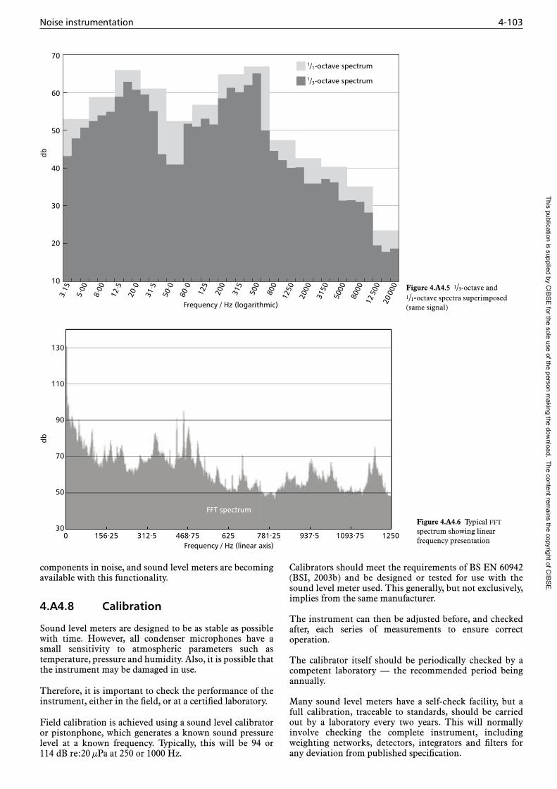
Noise instrumentation 4-103
components in noise, and sound level meters are becoming available with this functionality.
4.A4.8 Calibration
Sound level meters are designed to be as stable as possible with time. However, all condenser microphones have a small sensitivity to atmospheric parameters such as temperature, pressure and humidity. Also, it is possible that the instrument may be damaged in use.
Therefore, it is important to check the performance of the instrument, either in the field, or at a certified laboratory.
Field calibration is achieved using a sound level calibrator or pistonphone, which generates a known sound pressure level at a known frequency. Typically, this will be 94 or 114 dB re:20 µPa at 250 or 1000 Hz.
Calibrators should meet the requirements of BS EN 60942 (BSI, 2003b) and be designed or tested for use with the sound level meter used. This generally, but not exclusively, implies from the same manufacturer.
The instrument can then be adjusted before, and checked after, each series of measurements to ensure correct operation.
The calibrator itself should be periodically checked by a competent laboratory — the recommended period being annually.
Many sound level meters have a self-check facility, but a full calibration, traceable to standards, should be carried out by a laboratory every two years. This will normally involve checking the complete instrument, including weighting networks, detectors, integrators and filters for any deviation from published specification.
70
60
50
40
30
20
10
db
1/1-octave spectrum
Frequency / Hz (logarithmic)
1/3-octave spectrum
3.15
5·00
8·00
12·5
20·0
31·5
50·0
80·0
125
200
315
500
800
1250
2000
3150
5000
8000
12 5
0020
000 Figure 4.A4.5 1/3-octave and
1/1-octave spectra superimposed (same signal)
db
Frequency / Hz (linear axis)0 1250156·25 312·5 468·75 781·25625 1093·75937·5
130
110
90
70
50
30
FFT spectrum
Figure 4.A4.6 Typical fft spectrum showing linear frequency presentation
This publication is supplied by CIB
SE
for the sole use of the person making the dow
nload. The content remains the copyright of C
IBS
E.

4-104 Appendices
Appendix 4.A5: Vibration instrumentation
4.A5.1 Vibration parameters
Vibration is defined as the movement of a body or surface around a reference point over time. Vibration is most often characterised as acceleration, velocity or displacement, which are related as follows:
Velocity is the rate of change of displacement:
d x
v = — (4.A5.1) d t
Acceleration is the rate of change of velocity:
d x d x2
a = — = —– (4.A5.2) d t d t2
For the case of sinusoidal vibration, it is possible to convert acceleration, velocity and displacement levels using the following formulae:
displacement, x(t) = X sin (w t) (4.A5.3)
velocity, v(t) = w X cos (w t) (4.A5.4)
acceleration, a(t) = –w2 X sin (w t) (4.A5.5)
The most common parameter to be measured is acceleration, using an accelerometer, but sometimes velocity is measured directly using a geophone or seismometer.
Because of the above relationships, an integrator is often used to measure velocity and displacement from an accelerometer signal. This can take the form of an additional analogue conditioning device, or more recently, using digital techniques
As with sound level decibels, vibration can be expressed in decibels, and the reference level for acceleration is 10–6 m·s–2. Note however that some standards, particularly in the marine or military fields, use different reference levels, so care should be taken when reporting dB values.
The reference levels for velocity and displacement are 10–9 m·s–1 and 10–12 m respectively. This conveniently means that all three parameters expressed in decibels are numerically the same when w = 1000 rad·s–1 or 159.2 Hz, a frequency often used in vibration calibrators (see 4.A5.7)
Note that acceleration is often reported in units of g where 1 g = 9.81 m·s–2.
4.A5.2 Accelerometer
The most widely used vibration transducer is the piezoelectric accelerometer, due to its wide dynamic and frequency ranges.
The accelerometer consists of an internal seismic mass, mounted via a piezoceramic crystal on the base. This forms a single degree of freedom spring/mass/damper system.
Acceleration of the surface on which the accelerometer is mounted, causes acceleration of the base which in turn deforms the ceramic, which generates a proportional charge. This charge is then used to make the measurement.
The simple mass/spring/damper configuration has a resonance frequency, which is related to the seismic mass (typically small) and the ceramic stiffness (high). Therefore all accelerometers will show a high frequency peak in their response, which, due to the small damping, can be quite severe (~30 dB). However, if the accelerometer is used for measurements at least 3 times lower than this resonance, a nominally flat frequency response will be achieved.
The size of the accelerometer should be chosen so as not to affect the vibration of the measurement surface, i.e. as light as possible. However, a small accelerometer will have a low sensitivity, due to the smaller ceramic, but a larger accelerometer will have a lower resonant frequency. This makes selection of the correct accelerometer important.
The charge generated by the ceramic element is normally expressed as pC/m·s–2. The high output impedance of the ceramic means that a very high impedance charge amplifier must be used to transform this to a usable voltage for measurement purposes.
An external charge amplifier may be used, but more commonly, accelerometers now include the charge amplifier within the accelerometer case itself, using a system known as iepe (integrated electronic piezoelectric), which yields a voltage output proportional to acceleration. This amplifier can then drive standard co-axial cables to the measuring device, which must be able to provide the necessary power.
Accelerometers based on micro electromechanical systems (mems) are also starting to become widespread, offering much lower cost, without some of the drawbacks of piezo types.
4.A5.3 Vibration meter
A vibration meter takes the signal from the accelerometer, and measures the vibration, either as a root mean square (Rms) level or as a peak or peak-peak level.
The meter may also include filters (integrator) to enable readings of velocity or displacement.
As with the sound level meter, the energy average Leq may also be calculated, when the vibration level is varying with time.
A block diagram of a typical vibration meter is shown in Figure 4.A5.1.
Many sound level meters can also be used as vibration meters, making a convenient single instrument kit.
When integration to other parameters is used, it may be useful to apply a high-pass filter, to reduce the effect of unwanted electrical noise from cable movement or other
This publication is supplied by CIB
SE
for the sole use of the person making the dow
nload. The content remains the copyright of C
IBS
E.

Vibration instrumentation 4-105
environmental effects. This is because the integration effectively boosts low frequencies in the acceleration signal.
Measurements of acceleration are normally expressed as root mean square (Rms) values, but peak velocity measurements (ppv) are also often used for assessment of building damage.
For specialised measurements of vibration annoyance, a special root mean quad (Rmq) detector may be used. This results in the definition of vibration dose value (vdv) (m·s–1.75 ) as follows:
vdv = ∫
0
T a4(t) d t)0.25 (4.A5.5)
where a(t) is the acceleration in m·s–2 and T is the total measurement time in seconds. vdv is used in standards such as BS 6472 (BSI, 2008a) for vibration from traffic, trains etc.
4.A5.4 Weighting networks for human vibration
In order to assess the human effects of vibration, weighting networks are used in the same way as for sound level meters.
Human response to vibration is predominantly at low frequencies, and response depends on the direction of vibration — horizontal or vertical. BS EN ISO 8041 (BSI, 2005) specifies the standard filter networks, and for whole-body vibration, the Wd filter is used horizontally, and the Wb filter is used for vibration annoyance (see BS 6472). For health effects of vibration, the Wk filter is used in the vertical direction.
The Wb and Wd filter characteristics are shown in Figure 4.A5.2.
Sometimes it might be useful to also calculate the vector between the three orthogonal directions – lateral, frontal and vertical. Triaxial accelerometers are available, as are multichannel instruments, for measuring the three axes simultaneously.
For measurements of hand-arm vibration on e.g. power tools, the specialised Wh filter is used, and limits are defined in the European Physical Agents Directive (Vibration) (EC, 2002) for safe operation of handheld power tools.
4.A5.5 Accelerometer mounting
The correct mounting of accelerometers to the measurement surface is critical to ensure good measurements. If correctly mounted, the accelerometer will have a measurement range as specified in its documentation, to give a good frequency range, below its mounted resonant frequency.
However, if the accelerometer is not well mounted on the surface, then an additional mechanical interface will be introduced, which will add another resonance, typically within the frequency range of the measurement.
The correct mounting method is normally to drill and tap the surface, and stud mount the accelerometer with a specified torque.This is not always possible, so the following mounting methods can be used, in order of preference and efficacy:
AccelerometerIntegrator
Filters
Chargeamplifier
Peak
RMS
100 ms
Time weightings
Leq
∫
∫
∞
∞
10·4
Display
Detector
Weighting
HP2 Wb2...a2 d t
Figure 4.A5.1 Layout of a typical vibration meter
10
1
0·1
0·01
Gai
n
Frequency / Hz100
Wb (vertical)
Wd (horizontal)
0·1 1 10
Figure 4.A5.2 Wb and Wd weightings for respective vertical and horizontal whole-body vibration
This publication is supplied by CIB
SE
for the sole use of the person making the dow
nload. The content remains the copyright of C
IBS
E.

4-106 Appendices
— isocyanoacrylate/epoxy adhesive glued to accelerometer
— as above but using studded adhesive pad
— thin layer of beeswax
— magnet
— double-sided tape
— handheld probe.
The last two are to be avoided, unless only low frequency measurements are required. Typical frequency responses achieved using these methods are shown in Figure 4.A5.3.
4.A5.6 Frequency analysis
The most common form of frequency analysis used for vibration is ‘fast fourier transform’ (fft) analysis. This algorithm yields a series of constant bandwidth filters, spaced equally along a linear frequency axis.
fft analysis is an advanced application which is available on many handheld instruments, but the user should be familiar with the complexities before using it.
An advantage of fft analysis is that machine frequencies can be readily identified, and this can be used for troubleshooting sources of noise and vibration measured elsewhere in a building for example.
fft spectra can also be logged over a long period of time, so deteriorating machine condition can be identified and corrected before failure (condition monitoring).
Short-term fft monitoring can also be used for machine run-up/down, for identification of critical frequencies. This will aid the specification of machine mounts for example.
Other uses of frequency analysis include:
— measurements across vibration isolators to check performance
— investigating pipe vibration
— tracking sources of re-radiated noise elsewhere
— checking correlation between source vibration and end-user noise/vibration.
All these applications often require specialist advice.
4.A5.7 Calibration
To ensure the accuracy and reliability of measurements, the accelerometer and instrument should be calibrated before and after each series of measurements, or periodically at a test house. An accelerometer has the appearance of a tough steel transducer which is not easily damaged. The reverse is often the case, as the piezoceramic crystal can be easily cracked if the accelerometer is dropped on a concrete floor or generally mistreated. A cracked crystal will still provide an output, but it will not always be obvious there is any damage.
Field vibration calibrators are available, which are moving coil devices, generating a known vibration level at a fixed frequency. Typically, this frequency is chosen to be 159.2 Hz or 1,000 rads–1, so there is a convenient conversion between acceleration, velocity and displacement. For example, 10 ms–2 acceleration gives 10 mms–1 velocity and 10 µm displacement at 159.2 Hz
These calibrators tend to be expensive in relation to the cost of a vibration meter, so unless several vibration meters are used, then regular laboratory calibration may be preferred.
A single frequency calibrator will not necessarily show up a cracked piezo element, so a laboratory calibration will also check the frequency response of the complete system.
Care should also be taken of accelerometer cables, as damage can inject noise into the measurement.
Frequency / Hz
1Hand-held
probe
2Mountingmagnet
3Adhesive
4Isolated
stud
5Beeswax
6Threaded
stud
+ +
+
+ + +
1 2 3
4,5 6
28 k
31 k
12 k7 k
2 k
–30
0
–30Acc
eler
omet
er o
utpu
t / d
BFigure 4.A5.3 Different accelerometer mounting and its effect on frequency response
This publication is supplied by CIB
SE
for the sole use of the person making the dow
nload. The content remains the copyright of C
IBS
E.

Uncertainty in measurement and prediction of sound levels and sound power levels 4-107
Appendix 4.A6: Uncertainty in measurement and prediction of sound levels and sound power levels
4.A6.1 Measurement uncertainties
There is always an uncertainty associated with the measurement of any quantity. In the context of this Guide such uncertainties must be considered in relation to:
— acoustic data which is based upon acoustic measurements such as manufacturers’ sound power level, sound pressure level and silencer insertion loss data
— measurements of sound pressure levels carried out as part of commissioning and testing of building services systems.
Standards for the determination of sound power levels such as BS 848-1 (BSI, 2007) (for fans) or BS EN ISO 3744 (BSI, 2010d) (for machinery in general) give tables indicating typical uncertainties in various octave or ⅓-octave band levels and for overall dBA levels.
It should be noted that the low frequency octave bands (63 Hz and 125 Hz) will be subject to much higher levels of uncertainty (typically about 5 dBA) than higher octave band values and overall dBZ and dBA levels (typically 1 to 2 dBA). Manufacturers’ data for sound power levels should specify the test standard that has been used to determine the published values. The appropriate standard should be consulted to obtain the estimated uncertainty, bearing in mind that there are a range of measurement standards of varying accuracy, such as precision, engineering, survey, comparison etc., depending on the test procedure involved.
It should also be noted that not all published data are directly measured; some are either extrapolated or interpolated from measurements on representatives of a family of equipment types. Where sound power level data is presented with an uncertainty expressed as a standard deviation, the mean value plus one standard deviation should be used in the noise level prediction process.
Most recent (i.e. post 2000) standards relating to the measurement or prediction of noise levels contain a section on the estimation of uncertainties. These commonly relate to the methodology and terminology of ISO/IEC Guide 98-3: Uncertainty of measurement — Part 3: Guide to the expression of uncertainty in measurement (gum) (ISO, 2008), which takes a statistical approach to the estimation of uncertainty. The final or total uncertainty in a measurement result may include contributions from many different factors relating to, for example the measurement procedure, equipment and environmental conditions.
Although sound level measurements are limited by the accuracy of the measurement instrument (usually a sound level meter) in most cases this is a relatively small contributor to the total uncertainty in the measurement. The major sources of uncertainty are the variability of: the output of the sound source; the measurement position; sound propagation factors; and choices made by the human operator.
The gum gives a method for estimating these component uncertainties and aggregating them into a total or combined uncertainty. When this is expressed as a standards deviation it can be multiplied by a factor (k factor, or coverage factor) to provide and expanded uncertainty which may be related to a measurement confidence interval. A commonly used coverage factor, of 2, for example, gives an expanded uncertainty which represents a 95% confidence interval, so that there is a 95% chance that any measurement value will lie within one unexpanded uncertainty (in this case 2 standard deviations) of the mean of all measured values.
4.A6.2 Uncertainties in the prediction of noise levels
Uncertainties in predicted sound levels will arise from:
— from uncertainties in the input data
— uncertainties in the prediction method.
The accuracy of prediction of noise levels from building services is considered in section 6 of BS EN 12354-5 (BSI, 2009a) which states that:
As a global indication the expanded uncertainty for the single number ratings (A- or C-weighted levels) with a coverage factor of 2 could be estimated as up to 5 dB for the source input data and up to 5 dB for the transmission predictions; assuming these two aspects to be independent the overall expanded uncertainty would thus be up to 7 dB. Based on some global experience with comparable prediction schemes a more detailed overview of the estimated uncertainties is given. More research and comparison will be needed to be able to specify these uncertainties more accurately and in more detail.
Table 4.A6.1, taken from BS EN ISO 12354-5 (BSI, 2009a), indicates typical levels of uncertainty to be expected from the prediction of building services noise.
Suppliers of fans and silencers and of noise prediction software should be asked to supply estimates of uncertainty associated with the performance of their products.
Table 4.A6.1 Global estimate of the expanded uncertainty for various types of service equipment in buildings (source: BS EN ISO 12354-5 (BSI, 2009a))
Source type Source input data / dB Transmission / dB Remarks
All types 5 5 Lower values for heavy building structures
Ventilation systems 2 2
Heating installations 3 4
Lift installations 4 3
Water installations 3 5
Household equipment 3 3
This publication is supplied by CIB
SE
for the sole use of the person making the dow
nload. The content remains the copyright of C
IBS
E.

4-108 Appendices
Appendix 4.A7: Application of noise prediction software and integrated building design processes
4.A7.1 Noise prediction software
Most software prediction models of building services noise typically adopt algorithms, tables and formulae contained in this Guide. However, the complexity of each can vary significantly from simple spreadsheet-based models to more sophisticated numerical analysis packages incorporating 2D and 3D graphical outputs. The more complex the model, the more integrated the process can become and thus, if designed and used correctly, can be employed as a significant building services design tool. The purpose of this section is to highlight some of the advantages and potential pitfalls of both designing, validating and using such prediction models.
Prediction software is becoming increasingly employed by building services acousticians to calculate both internal room noise levels and external noise impacts. When using prediction models, care should be taken to check that source data and noise pathways are accurately replicated from engineering drawings, thereby ensuring accurate results can be obtained.
Source noise parameters (when obtained from manufac-turers’ accredited test data) must be in a format, which is identical to that which the prediction model requires. In addition, the insertion losses of specific attenuation measures should be checked against those defined in specifications to maintain consistency throughout the design process.
Currently, a number of commercially available computer prediction packages exist which provide a reasonably high level of accuracy. However, before complete confidence can be afforded to the use of such packages, initial verification of the prediction software’s calibration against real-life acoustic systems should be sought. Software developers should aim to provide accredited calibration data of their prediction models when tested against laboratory systems of known operating and load conditions. A typical level of calibrated accuracy of a noise prediction package should lie within ±3 dB of a laboratory test system which should include a number of services elements (e.g. for ducted systems: straight sections, bends, transformations, branches, plenums and air terminal devices into known room acoustic conditions). Computer prediction models which have no specified level of uncertainty, should be used cautiously under ‘worst case’ operating conditions, to account for a higher likelihood of calculation inaccuracy.
Some outline considerations for use of noise prediction software:
— Although widely employed, caution should be taken to correctly validate results.
— Models should be programmed using known, reputable and published algorithms e.g. CIBSE or ASHRAE (or similarly approved international guidance). All sources must be referenced.
— There should be some estimate of uncertainty relating to results, distinguishing between
uncertainty in the input data and that inherent in the prediction process.
— Users are encouraged to compare results obtained between different software packages using the same input data and system design thereby instilling a greater level of confidence.
— Users should also have sufficient familiarity and expertise in the subject matter to make critical judgments about the validity and robustness of the final results.
— It is advisable to conduct sensitivity analyses on a design model when using software packages to estimate the effects on result uncertainty by varying input parameters.
4.A7.2 Integrated building design
In recent years, there has been a growing trend towards integrating building design systems into a more holistic process. Such a process has been in development internationally for some time and is currently referred to as building information modelling (bim). The development of bim has been heralded as a method of adopting a fully integrated design process for the wider construction industry.
One of the main drivers for this development has been to aid stakeholders and designers alike to better predict (and thus manage) the building performance, capital and lifetime costs as well as any environmental impacts inherent in the building design process. At the design level, one of bim’s benefits is that it enables each member of the design team to visualise the specification, integration, construction detailing and costing for any discrete building system element. In addition, this process should also facilitate the early identification of potential conflicts between design elements.
While many engineering disciplines have been quick to engage in new technology supporting this development, this should be viewed as an opportunity for the noise and vibration performance of building services to be integrated into the process. Following recent regulatory changes to building performance criteria, notably to improve energy efficiency and reduce carbon emissions, noise and vibration performance should therefore be assessed on equal merit.
This consideration is ever more apparent with the emergence of renewable technologies which serve to achieve regulatory energy efficiency and low carbon performance criteria. As such, where a renewable technology is known to exhibit significant levels of noise or vibration, these should also be evaluated in an integrated design process under the same scrutiny as for other building performance criteria (e.g. energy efficiency, ventilation, thermal, lighting).
Building services noise prediction software, whether integrated into a global design package or when employed as a standalone tool, should therefore facilitate the collection
This publication is supplied by CIB
SE
for the sole use of the person making the dow
nload. The content remains the copyright of C
IBS
E.

Glossary 4-109
and classification of source noise data from any existing or emerging technology. There are a number of existing standards which relate to the estimation of building services noise such as; BS EN 12354-5 (2009a). It is therefore advisable that any integrated design package which incorporates a noise element, should be based on algorithms and estimation methods contained in such approved standards.
More information on integrated building design processes and bim in particular, can be found online:
— www.cabinetoffice.gov.uk/resource-library/government-construction-strategy: the UK Government online resource defining its construction strategy earmarking future implementation of bim.
— www.bimtaskgroup.org: the Building Information Modelling Task Group is supporting and helping deliver the objectives of the Government Construction Strategy through a collaborative implementation of the bim process.
— www.buildingsmart.com: a neutral, international not-for-profit alliance of organisations supporting openbim; an open-source bim protocol. There are regional chapters in Europe, North America, Australia, Asia and the Middle East.
— www.cibse.org/bim: the CIBSE BIM Steering Group is actively linked in with the work of the UK Government’s BIM Task Group and is liaising with many of the ‘BIM4’ groups.
Appendix 4.A8: Glossary
Absorption: The conversion of sound energy into heat as a result of some frictional process occurring within a sound absorbing material. The amount of absorption provided by a surface is quantified as the amount of absorption, A, in m2
as the equivalent area of perfect absorber the product of the surface area.
Absorption coefficient: The ratio of the acoustic energy absorbed by a surface exposed to a sound field to the acoustic energy incident upon it. It is a number between 0 (perfect reflector, i.e. zero absorption) and 1 (perfect absorber).
Acoustic impedance: The complex ratio of the sound pressure to the volume velocity through a chosen surface.
Acoustics: Acoustics is (a) the science of sound, including its production, transmission, and effects, or (b) the qualities that determine the value of a room or other enclosed space with respect to hearing.
Aerodynamic noise: Noise in a fluid arising from fluctuating fluid flow. Examples are noise produced by fans, jets valves.
Ambient noise: A combination of sounds from many sources, associated with a given environment. For example ambient noise in offices consists of noise from building services, intrusion of external noise and occupancy noise.
Amplitude: The peak value of a fluctuating quantity from its mean value.
Anechoic room: A room designed to simulate free field conditions for sound propagation. Anechoic rooms are used for testing of equipment to measure sound power levels, and also directivity ratio/index of noise sources.
Attenuation: The loss or reduction in magnitude of a signal. The amount by which a noise control device such as a silencer or enclosure reduces noise levels expressed in decibels.
A-weighting: A frequency weighting widely used in sound measurement equipment, devised to take into account the fact that human response to sound is not equally sensitive to all frequencies defined in BS EN 61672-1 (BSI, 2013c).
A-weighted sound level: A single figure measured on a specific scale, which can be related to the subjective assessment of the loudness of a noise.
Background noise: Sound other than the wanted signal under investigation. Background noise is often described and measured as the 90th percentile level, in dBA: LA90.
Band sound pressure level: The total sound pressure level for the sound energy contained within a specified frequency band (e.g. octave sound pressure level).
Bandwidth: The difference between the upper and lower frequency limits typically of a filter.
Coincidence frequency: That frequency of an incident sound whose projected wavelength at a particular angle coincides with the corresponding bending waves of the sound in a plate. Below their critical frequency, plates and panels (e.g. walls and floors) are good sound insulators but there is often a dip in sound insulation above the critical frequency.
C-weighting: A frequency weighting widely used in sound measurement equipment, devised to take into account the fact that human response to sound is not equally sensitive to all frequencies defined in BS EN 61672-1 (BSI, 2013c), see Appendix 4.A4. The difference between dBC and dBA is often used as an indicator of low frequency content of a noise. See section 4.9, and also CIBSE Guide A (2015b) section 1.10.
D, DnT and Dn,e: These are the level difference, the standardised level difference, and the element normalised level difference. Measures of the sound insulation performance of a building element. See section 7. Defined in BS EN ISO 10140-2 (BSI, 2010b). Usually measured in 16 ⅓-octave frequency bands from 100 Hz to 3150 Hz.
Dw, DnT,w and Dn,e,w: Weighted single figure versions of the above defined according to BS EN ISO 717-1 (BSI, 2013a).
Damping: The process whereby the amplitude of oscillation of a system is diminished.
Decibel scale: A decibel scale is a logarithmic scale for comparing the ratios of two powers (e.g. electric power or
This publication is supplied by CIB
SE
for the sole use of the person making the dow
nload. The content remains the copyright of C
IBS
E.

4-110 Appendices
sound power) or quantities which are related to power (e.g. sound pressure). In order to create absolute scales a base or reference value is defined. In this Guide the sound pressure level and sound power level are commonly referred to (and defined later in this glossary) with reference values of 1 × 10–12 W (for the sound power level scale) and 2 × 10⁻⁵ Pa (for the sound pressure level scale). See also Appendix 4.A1.
Diffuse sound field: A sound field of uniform energy density for which the direction of propagation of waves are random.
Diffusion: The degree to which the direction of propagation of waves is random. Diffuse surfaces reflect sound in a random manner and help to avoid standing waves which can arise with specular reflection (i.e. which obey the laws of reflection).
Direct field: That part of the sound field of a source wherein the effects of the boundaries of the medium can be neglected.
Directivity factor: The ratio of the sound pressure squared of the radiated sound in a particular direction at any remote point on a reference axis to the average sound pressure squared for all directions in space at the same distance from the sound source. (See Appendix 4.A1 for explanation and sections 4.4 and 4.10 for application).
Directivity index: The difference between the sound pressure level of the radiated sound in a particular direction at any remote point on a reference axis to the average sound pressure level for all directions in space at the same distance from the sound source. (See Appendix 4.A1 for explanation and sections 4.4 and 4.10 for application).
Equivalent absorption area: The equivalent area of a surface for which the absorption is unity, which then absorbs the same quantity of acoustic energy as the objects under consideration.
Equivalent noise exposure level Leq: A single figure average of sound level derived from the total sound energy received over a given period of time. Its calculation involves the conversion of sound pressure levels to sound energy units received, with respect to time, and the conversion of the mean total energy to sound pressure level in dB (A).
Far field: That part of the sound field from a radiating source in free field conditions wherein the sound pressure level diminishes at 6 dB per doubling of distance.
Flanking transmission: The transmission of sound between two rooms by any indirect path of sound transmission other than through the partition between the rooms.
Free field: A sound field in which the effects of the boundaries are negligible. Applies to tests carried out in an anechoic room or approximately to outdoor sound propagation. In free field conditions the sound pressure level from a sound source decrease with distance at a rate of 6 dB per doubling of distance. See Appendix 4.A1.
Frequency: The rate of repetition of the cycles of a periodic quantity. The unit is the hertz (Hz).
Fundamental frequency: The lowest natural frequency of an oscillating system.
Frequency analyser: An instrument for measuring the band pressure level of a sound or vibration at various frequencies.
Frequency analysis: The measurement of band pressure levels of a sound or vibration at various frequencies.
Harmonic: A sinusoidal component of a periodic wave form having a frequency which is an integral multiple of the fundamental frequency.
Hertz: A unit of frequency: 1 Hz = 1 cycle per second.
High pass filter: A filter that transmits energy at all frequencies above a certain frequency, and attenuates all lower frequencies.
Impulsive noise: A noise of short time duration and which may be repeated at regular intervals.
Insertion loss: A measure of the effectiveness of noise control devices such as attenuators and enclosures; the insertion loss of a device is the difference, in dB, between the noise level with and without the device present.
Isolation efficiency: A measure of the effectiveness of a vibration isolation system; isolation efficiency = (1 – T) × 100%, where T is the transmissibility of the system; see also under transmissibility.
Level: The word level implies the use of a decibel scale, e.g. sound pressure level in decibels, sound pressure in pascals.
Level difference, D: The difference in level between two rooms and the basic measure of airborne sound insulation in BS EN ISO 10140 (BSI, 2010a/b).
Line spectrum: The spectrum of a sound, the components of which occur only at a number of pure tones.
Longitudinal wave: A wave in which the particle displacement at each point of the medium is parallel to the direction of wave travel.
Loudness: An observer’s subjective auditory impression of the strength of sound. See Appendix 4.A1 and CIBSE Guide A (2015b) section 1.10.
Loudness level: The sound pressure level of a 1000 Hz pure tone which on comparison is assessed by normal observers as being equally as loud as the sound being measured. Measured in phons.
Low pass filter: A filter which transmits energy at all frequencies below a certain frequency and attenuates at all higher frequencies.
Masking: The amount by which the threshold of audibility of a sound is raised by the presence of another sound.
Measurement surface: A defined geometric surface on which noise measurements may be made. An example would be an imaginary surface surrounding a machine in an anechoic room over which sound pressure level measurements are made in order to determine the sound power level of the machine
Microphone: An electro-acoustic transducer that converts an acoustical signal to an electrical signal.
This publication is supplied by CIB
SE
for the sole use of the person making the dow
nload. The content remains the copyright of C
IBS
E.

Glossary 4-111
Microphone–condenser: A microphone in which the transducing function is achieved from variations in the electrical capacitance of its elements.
Natural frequency: The frequency of a freely vibrating system.
Near field: That part of a sound field near to a source radiating sound in free-field conditions wherein the sound pressure and particle velocity are not in phase. A region close to a sound source, e.g. a compressor or generator, where it is not easy to predict how the sound level varies with distance from the source (and the 6 dB per doubling of distance rule does not apply).
Noise: Commonly defined as unwanted sound.
Noise criteria (Nc) curves: A method for rating or assessing internal (mainly office) noise; it consists of a set of curves relating octave-band sound pressure level to octave-band centre frequencies; each curve is given an Nc number, which is numerically equal to its value at 1000 Hz (see section 4.9).
Noise rating (NR) curves: A similar method for rating noise, based on octave band sound pressure levels to the Nc system (refer to section 4.9).
Octave: A bandwidth for which the upper limiting frequency is equal to twice that of the lower limiting frequency. In this guide noise levels in the octave band range from 63–8000 Hz are commonly used.
Octave and ⅓-octave bands: These are sets of frequency bands of constant percentage bandwidth used for frequency analysis of sounds. For octave bands the upper limiting frequency is equal to twice that of the lower limiting frequency. In this guide noise levels in the octave band range from 63–8000 Hz are commonly used: 63, 125, 250, 500, 1000, 2000 and 8000 Hz. Although octave band analysis is the usual form of frequency analysis used in this Guide, ⅓-octave bands are sometimes used, for example for sound insulation measurements. For ⅓-octave bands the upper limiting frequency is equal to 1.22 times the lower limiting frequency. Also see Appendix 4.A4.
Peak value: The maximum numerical value attained for a varying quantity. The peak value of sound pressure level is used in the ‘exposure action values’ of the Control of Noise at Work Regulations 2005 (TSO, 2005) (see section 4.4)
Pistonphone: An instrument in which a piston vibrates at known frequency and amplitude, whereby the resulting sound pressure level within the cavity can be specified. Used for microphone calibration. See Appendix 4.A4.
Plane wave: An idealized model of sound propagation where the wave fronts are plane and parallel everywhere so that the sound energy does not diverge with increasing distance from the source (which is the case for spherical waves).
Pure tone: A sound in which the sound pressure level varies sinusoidally with time, i.e. a single frequency. Sometimes machinery has tonal components which make this type of noise more annoying.
Random incidence absorption coefficient: The sound absorption coefficient when the surface or material is exposed to a diffuse sound field and is the usual measure of the sound absorption performance of materials.
Random noise: Noise due to the combination of a large number of elementary disturbances with random occurrence in time.
Regenerated noise: A secondary source of noise (i.e. other than the fan) which is caused by turbulent air or water flow through a fitting or device.
Resonance: Occurs when the frequency of the excitation coincides with the natural frequency of a vibrating system.
Reverberant field: A sound field resulting from the super-position of many sound waves due to repeated reflections at boundaries. Referred to in section 4.7.
Reverberation: The persistence of sound due to repeated reflection at the boundaries.
Reverberation room: A sound measuring room specially designed to facilitate the production of diffuse sound fields. Can be used for the measurement of sound power levels of machinery, but, unlike tests in an anechoic room cannot be used to determine directivity of sources.
Reverberation time: The reverberation time is the time required for the average sound intensity level, originally in a steady state, to decrease after the source is stopped to one millionth of its intensity i.e. 60 dB. In this guide the reverberation time is used as an indication of the amount of sound absorption, i.e. rooms with very little absorption have large reverberation times, whereas rooms with a lot of sound absorption have small reverberation times. The relationship between reverberation time and absorption is given by Sabine’s formula, used in section 4.7.
Room constant: Room constant = S a / (1 – a), where S is the total surface area of the room, including objects in the room and a is the average absorption coefficient of these surfaces. Used in sections 4.7 and 4.10. It is a measure of the importance of reverberation in a room, so that in a ‘dead’ room the room constant will be small.
Root mean square, Rms: The Rms value of a set of numbers is the square root of the average of their squares; for a sound or vibration waveform the Rms value over a given time period is the square root of the average of the square of the waveform over that time period. The Rms sound pressure level is the most commonly used measure of the average of sound pressure level.
Room criterion, Rc: A single figure method for rating and assessing a noise which like the NR and Nc methods is based upon octave bands but which takes into account the shape of the spectrum.
Sabine’s formula: A formula that relates the reverberation time, T (s), of a room with the room volume, V (m3), and amount of absorption, A (m2), contained within the room:
T = 0.16 V / A
Silencer: A commonly-used term for an attenuator.
This publication is supplied by CIB
SE
for the sole use of the person making the dow
nload. The content remains the copyright of C
IBS
E.

4-112 Appendices
level in the 250 Hz octave band exceeds any of these bands by 10 dB or more then this value is also included.
Speed of sound: The velocity at which sound travels in an elastic medium. Within air it is usually taken as 330–340 m/s depending upon temperature.
Spherical wave: A wave in which the wave fronts are concentric spheres so that sound pressure level reduces with distance in accordance with the inverse square law. See Appendix 4.A1.
Spring rate: The rate of a spring is the amount it will deflect per kilogram of applied load imposed. Also known as spring stiffness. See section 4.11.
Spring stiffness: In practical vibration isolation, the spring stiffness is expressed as the spring rate (kg/mm), which describes the load in kilograms required to deflect a spring by 1 mm. Also known as spring rate. See section 4.11.
Standing wave: Periodic wave having a fixed distribution in space which is the result of interference between progressive waves travelling in opposite directions and of the same frequency. Such waves are characterized by the existence of maxima and minima that are fixed in space.
Structure-borne noise: Noise which is propagated by the vibration of a solid structure.
Third octave: Band of frequencies for which the upper limiting frequency f2 is equal to 1.25 × the lower limiting frequency fl. Therefore: f2 = 1.25 fl.
Threshold of hearing: The lowest sound pressure at a given frequency that the human ear can detect.
Threshold of pain: The sound pressure at a given frequency above which a person experiences physical pain.
Tone: Sound containing only a distinctive narrow band of frequencies.
Transmissibility: Of a vibrating system; the non-dimensional ratio of vibration amplitude at two points in the system; frequently, the two points are on either side of springs used as anti-vibration mounts, and the transmissibility is used as an indicator of the effectiveness of the isolation.
Transmission loss: See sound reduction index.
Vibration: A to and fro motion; a motion which oscillates about a fixed position.
Weighted sound reduction index, Rw: A single figure value derived from 16 ⅓-octave band values of sound reduction index (from 100 Hz to 3150 Hz) using the procedure described in BS EN ISO 717-1 (BSI, 2013a).
Wavelength: The perpendicular distance between two wave fronts in which the phases differ by one complete period. Wavelength is equal to the phase velocity divided by the frequency.
Z-frequency weighting: Zero frequency weighting, defined in BS EN ISO 61672-1 (BSI, 2013c) in which the weighting is zero in all frequency bands, i.e. a flat frequency response. See Appendix 4.A4.
Sound absorbing material: Material possessing a relatively high sound absorption coefficient. Sound absorbing materials are used to reduce reflections by room surfaces and thus to reduce reverberation in rooms.
Sound absorption: The process by which sound energy is progressively diminished in passing through a medium, or diminished in striking a surface due to internal energy loss. See under absorption.
Sound insulation: A measure of the reduction of sound between two locations, or more usually the reduction or attenuation of airborne sound by a solid partition between source and receiver; this may be a building partition (e.g. a floor, wall or ceiling), a screen or barrier, or an acoustic enclosure. The sound insulation performance of a building element (wall floor, door, window etc.) is specified in terms of its sound reduction index, also known as it transmission loss.
Sound level meter: An instrument designed to measure a value of the sound pressure level, which may be frequency weighted. See Appendix 4.A4.
Sound power: The total sound energy radiated per unit time by a sound source, measured in watts.
Sound power level: The sound power of a sound source expressed in decibels. It is 10 times the logarithm to the base 10 of the ratio of the sound power of the source to the reference power of 10–12 W. Sound power levels are determined by measuring the sound pressure levels produced by the sound source in a special test room; either an anechoic room or a reverberant room.
Sound power level spectrum: The spectrum of a sound expressed in terms of sound power levels per stated bandwidth.
Sound pressure: The alternating component of the pressure at a point in a sound field.
Sound pressure level: In decibels, 20 times the logarithm to the base 10 of the ratio of the sound pressure to the reference pressure of 2 × 10⁻⁵ Pa for air.
Sound pressure level spectrum: The spectrum of a sound expressed in terms of the sound pressure level per stated bandwidth.
Sound propagation: The wave process whereby sound energy is transferred from one part of a medium to another.
Sound reduction index: In decibels, is 10 times the logarithm to the base 10 of the ratio of the sound energy incident upon a surface to that transmitted through and beyond the partition. Also known as transmission loss. Determined by measurements in accordance with BS EN ISO 10140 (BSI, 2010a/b).
Sound transmission: The transfer of sound energy from one medium to another.
Speech interference level: This provides a method of rating steady noise according to its ability to interfere with conversation between two people. It is calculated from the arithmetic average of the sound pressure levels of the noise measured in the 500, 1000 and 2000 Hz octave bands. If the
This publication is supplied by CIB
SE
for the sole use of the person making the dow
nload. The content remains the copyright of C
IBS
E.
Summary 4-113
IndexNote: page numbers in italics refer to figures; page numbers in bold refer to tables
acceleration 4-70, 4-104accelerometers 4-104, 4-105 to 4-106acoustic concepts 4-90 to 4-96acoustic louvres 4-20 to 4-21acoustic screening 4-59acoustic ventilators 4-59, 4-60active attenuators 4-45 to 4-46active beams 4-23 to 4-24air compressors 4-21, 4-30, 4-74air conditioning units 4-13 to 4-14air exhaust outlet grilles 4-18air extract ductwork 4-8air handling units 4-17 to 4-18, 4-74air intakes 4-18, 4-19, 4-59air springs 4-79air supply ductwork 4-8air supply fan assemblies 4-19air supply grills 4-32air terminal units 4-8 to 4-11
casing breakout noise 4-8 to 4-9dual duct units 4-9extract applications 4-8inlet sound power levels 4-8manufacturers’ data 4-9, 4-10outlet sound power levels 4-8position 4-55variable air volume (VAV) units 4-9
air vents 4-57, 4-59, 4-60airflow noise 4-29 to 4-35, 4-31, 4-96 to 4-98airflow velocity 4-30 to 4-31, 4-32architectural considerations 4-70attenuators see noise attenuatorsaudible warnings and announcements 4-25axial flow fans 4-7
close coupled circular attenuators 4-43, 4-44
noise spectrum 4-43rooftop air handling units 4-17 to 4-18vibration isolation 4-74
balancing dampers 4-9, 4-13, 4-18balancing of rotating machinery 4-73blade frequency increments (BFI) 4-6, 4-7boilers 4-21, 4-22
rooftop air handling units 4-18typical noise levels 4-30vibration isolation 4-74
BREEAM 4-61broad band noise 4-90building design considerations
floating floors 4-70, 4-79 to 4-80, 4-86 to 4-87
structural bearings 4-80vibration avoidance 4-70vibration isolation 4-75
building information modelling (BIM) 4-108 to 4-109
Building Regulations, Part E 4-56
casing breakout noiseaxial flow fans 4-17centrifugal fans 4-6, 4-7control valves 4-8 to 4-9fan coil units 4-11
cavitation 4-27centrifugal compressors 4-21, 4-30centrifugal fans 4-6, 4-7, 4-18, 4-43, 4-74
chilled ceilings 4-22 to 4-24chillers 4-21, 4-30, 4-74circular ductwork 4-47 to 4-48, 4-49, 4-51close coupled circular attenuators 4-43, 4-44close-coupled secondary attenuators 4-8commercial catalogue data see manufacturers’
datacompressors see air compressorscondensing units 4-17constant volume (CV) 4-8Control of Noise at Work Regulations 2005
4-27 to 4-28control valves 4-8 to 4-9, 4-26 to 4-27cooling coils 4-8cooling towers 4-17, 4-22, 4-23
typical noise levels 4-30vibration isolation 4-74, 4-84 to 4-86
cross-talk 4-57 to 4-58
dampers 4-33damping 4-71 to 4-72, 4-72dBA 4-61dBC 4-61decibel scale 4-91, 4-91 to 4-92, 4-95, 4-96degrees of freedom 4-80design criteria 4-61diesel engines 4-30diffusers 4-9, 4-11, 4-35, 4-98, 4-98directionality 4-93directivity factor 4-93 to 4-94directivity index 4-94dissipative attenuators see passive attenuatorsdisturbing frequency 4-71domestic appliances 4-27dry air cooling towers 4-17ductwork
acoustic lining 4-36, 4-46, 4-60, B4-37 to B4-38, B4-39
airflow noise 4-29 to 4-35, 4-31, 4-96 to 4-98
airflow velocity 4-30 to 4-31, 4-32bends 4-31, 4-36, 4-39, 4-96, B4-39branches 4-39, 4-96break-in noise 4-48 to 4-51, 4-50, 4-51,
4-67breakout noise 4-29, 4-46 to 4-48, 4-66 to
4-67circular 4-47 to 4-48, 4-49, 4-51contractions 4-31duct length effect 4-46 to 4-47, 4-48duct rumble 4-32, 4-34ducted feeds through the roof slab 4-19end reflection loss 4-39 to 4-40, 4-40flexible connectors 4-79hangers 4-79in-duct attenuators 4-8, 4-20, 4-29, 4-31,
4-32, 4-32, 4-35, 4-40lagging/cladding 4-50 to 4-51, 4-51location 4-49, 4-49materials 4-36noise attenuation 4-36 to 4-46oval or ‘flattened’ circular 4-47plate dampers 4-34 to 4-35pressure loss 4-96rectangular sheet metal 4-46 to 4-47, 4-48,
4-50sound power and pressure levels 4-94system attenuation requirements 4-65 to
4-66, 4-66system noise prediction 4-65 to 4-66terminations 4-98turbulence-induced noise 4-31 to 4-35vibration isolation 4-86
elastomeric materials 4-76 to 4-77elastomer-in-shear 4-78, 4-82electric motors 4-26, 4-26elevators see liftsescalators 4-25 to 4-26external noise 4-59 to 4-60extract grills 4-32extract ventilators 4-8, 4-19
fan coil units 4-11 to 4-12fan-assisted terminal units 4-14, 4-15, 4-16fans 4-6 to 4-8
air supply fan assemblies 4-19blade frequency increments (BFI) 4-6, 4-7typical noise levels 4-30vibration isolation 4-74, 4-82
fast fourier transform (FFT) analysis 4-102, 4-103, 4-106
fibrous sound absorbing materials 4-46flexible circular duct attenuators 4-43, 4-45flexible pipe connectors 4-79floating floors 4-70, 4-79 to 4-80, 4-86 to 4-87floor slabs 4-75flow straighteners 4-31 to 4-32fragility levels 4-70, 4-76frequency analysis 4-3, 4-102fridge compressor units 4-18
gas turbines 4-74gas-fired boilers 4-18glazing 4-57glossary 4-109 to 4-112grilles 4-9, 4-11, 4-32, 4-35, 4-36
hangers 4-79, 4-86heat rejection plant 4-22helical springs 4-78, 4-82human response to sound 4-92, 4-101human response to vibration 4-73, 4-105
induction units 4-12 to 4-13inertia bases 4-78 to 4-79insertion losses
close-coupled axial fan attenuators 4-44in-duct attenuators 4-40, 4-41, 4-43, 4-45lagging/cladding materials 4-51plenums 4-43
instrumentationnoise measurement 4-100 to 4-103vibration measurement 4-104 to 4-106
internal combustion engines 4-30, 4-74internal walls 4-57isolation hangers 4-79isolator rails 4-84 to 4-86
lagging/cladding 4-50 to 4-51, 4-51lifts 4-24 to 4-25louvres see acoustic louvres
manufacturers’ data 4-2, 4-5, 4-99masonry walls 4-57measurement
noise measurement 4-100 to 4-103uncertainties 4-107vibration measurement 4-104 to 4-106
mixed flow fans 4-43mixing boxes 4-9motors, electric see electric motorsmounts
load determination 4-82 to 4-83number and location 4-80 to 4-81types 4-82
natural frequency 4-71, 4-76natural ventilation 4-59 to 4-60
This publication is supplied by CIB
SE
for the sole use of the person making the dow
nload. The content remains the copyright of C
IBS
E.

4-114 Noise and vibration control for building services systems
NC levels 4-62neoprene pads 4-77noise attenuators
active 4-45 to 4-46air handling units 4-18axial flow fans 4-43, 4-44in-duct attenuators 4-8, 4-20, 4-29, 4-31,
4-32, 4-35, 4-40noise break-in 4-51 to 4-52, 4-52self-generated noise B1-32
noise control (general guidance) 4-5, 4-88noise conversion efficiency 4-3noise criteria 4-60 to 4-62noise emission data 4-2noise exposure levels 4-28noise generation mechanisms 4-1noise induced hearing loss 4-27 to 4-28noise levels prediction 4-63 to 4-69
airflow noise 4-63 to 4-69breakout/break-in noise 4-66 to 4-67duct system 4-65 to 4-66, 4-66noise propagation to outdoors 4-67 to 4-69,
4-69room effect 4-63 to 4-64, 4-64, 4-65software 4-108uncertainties 4-107
noise measurement 4-100 to 4-103noise propagation to outside 4-59 to 4-60
plant rooms 4-28 to 4-29prediction 4-67 to 4-69, 4-69rooftop units 4-20split air conditioning units 4-13 to 4-14
noise quality 4-61noise ratings (NR values) 4-25, 4-61 to 4-62
ductwork 4-32grilles and diffusers 4-35, 4-36
noise sources 4-3, 4-5 to 4-27noise spectrum 4-90noise transmission paths 4-3 to 4-5
occupant comfortprivacy and cross talk 4-57 to 4-58vibration control 4-73, 4-75
octave analysis 4-3, 4-102, 4-103oil-fired boilers 4-18openable windows 4-59out-of-balance forces 4-73oval or ‘flattened’ circular ductwork 4-47
pad materials 4-76 to 4-78partitions 4-57passive attenuators 4-40, 4-41, 4-42passive beams 4-22 to 4-23passive panels 4-23perforated plates 4-34 to 4-35pipework 4-27
flexible connectors 4-79hangers 4-79, 4-86vibration isolation 4-86water hammer 4-27
plant roomsbreakout noise 4-28 to 4-29, 4-56estimation of noise levels 4-29noise exposure levels 4-27 to 4-28typical noise levels 4-30
plate dampers 4-34 to 4-35
plenums 4-43 to 4-44polychloroprene pads 4-77power ratio 4-91pressure loss
acoustic louvres 4-21dampers 4-33ductwork 4-96in-duct attenuators 4-40passive attenuators 4-42
pressure loss factor 4-96pressure reducing valves (PRVs) 4-8pressure safety valves (PSVs) 4-27privacy 4-57 to 4-58pumps 4-21, 4-26
cavitation 4-27rooftop air handling units 4-18typical noise levels 4-30vibration isolation 4-74
quality index (QI) 4-61
radiators 4-23reciprocating compressors 4-18, 4-21, 4-30rectangular sheet metal ductwork 4-46 to 4-47,
4-48, 4-50refrigeration plant 4-74regulations 4-27 to 4-28reheat coils 4-8reverberation 4-28, 4-52 to 4-53, 4-93rooftop units 4-17 to 4-20room constant 4-52room sound levels 4-52 to 4-58
acoustic considerations 4-93prediction 4-63 to 4-64, 4-64, 4-65privacy and cross talk 4-57 to 4-58sound absorption coefficients 4-53sound level determination at a receiver point
4-52 to 4-54sound transmission between rooms 4-56
to 4-57source directivity 4-55, 4-55 to 4-56
rotary vane refrigerant compressors 4-18
Schultz method 4-54, 4-64, 4-65screening see acoustic screeningscrew compressors 4-21sensitivity tests 4-69separating walls 4-57silencers see noise attenuatorsskids 4-78, 4-81software 4-108sound absorbing materials 4-36, 4-46sound energy 4-91sound frequency, wavelength and velocity 4-90
to 4-91sound intensity 4-91sound intensity level 4-92sound level meters 4-100 to 4-101, 4-103sound power levels 4-91 to 4-93sound pressure 4-90, 4-91, 4-93sound pressure levels g, 4-92
decibel scale 4-91, 4-91 to 4-92, 4-94 to 4-96, 4-95, 4-96
equivalent continuous 4-101 to 4-102in rooms 4-92 to 4-93variation with distance 4-93
sound reduction index 4-57, 4-57sound transmission loss see sound reduction
indexsplit air conditioning units 4-13 to 4-14spring hangers 4-79spring rate 4-71, 4-75stack ventilation systems 4-60standby generators 4-19, 4-74static deflection 4-71, 4-75statistical levels 4-102steam boilers see boilersStrouhal number 4-97structural bearings 4-80structural considerations 4-70, 4-75suspended ceilings 4-8 to 4-9
through-the-wall air conditioning units 4-13 to 4-14
tonal components 4-90, 4-102traffic noise 4-61trickle ventilators 4-59turbulent air flow 4-29 to 4-30, 4-31 to 4-35turbulent water flow 4-26
uncertainty in measurement and prediction 4-107
variable air volume (VAV) 4-8vibration control 4-69 to 4-87
damping 4-71 to 4-72, 4-72fundamentals 4-70 to 4-71mechanical isolation 4-70relation between vibration quantities 4-71transmissibility 4-71, 4-72
vibration emission ratings 4-72 to 4-73, 4-76vibration frequency analysis 4-106vibration instrumentation 4-104 to 4-106vibration isolation
criteria 4-73 to 4-76equipment performance requirements 4-73
to 4-75, 4-74interface with building structure 4-75 to
4-76plant room equipment 4-28practical examples 4-80 to 4-87rooftop air handling units 4-19
vibration isolation efficiency (VIE) 4-72, 4-73, 4-75
vibration isolators 4-75 to 4-76vibration measurement 4-104 to 4-106vibration meters 4-104 to 4-105vibration parameters 4-104vibration rating of machinery 4-72 to 4-73,
4-76
waste water installations 4-27water flow noise 4-26 to 4-27water hammer 4-27water-cooled cooling towers 4-17watts (W) 4-91wavelength, frequency and velocity 4-90 to
4-91‘windcatcher’ ventilators 4-60windows 4-57
This publication is supplied by CIB
SE
for the sole use of the person making the dow
nload. The content remains the copyright of C
IBS
E.