No/Low-Cost Ways to Drive Savings Today Using Real-Time Energy Data

Introduction

Most facilities staff and energy managers have two things in common: 1) they don’t have enough time, and 2) they don’t have enough money to spend on projects that would improve the operating efficiency of their buildings. This eBook is designed to help those weary champions of operational excellence by outlining five Energy Efficiency Measures (EEMs) that require little or no capital investment, improve (or at least are neutral to) occupant comfort, and help build momentum within a company that a savvy energy manager can parlay into funding for more capital intensive projects.

To make sure we’re all on the same page, we’re defining a “no/low-cost Energy Efficiency Measure” as a corrective action with a payback of less than two years. Even the most hard-nosed CFO has to like those economics. Each measure addresses one of the 3 energy cost drivers: how you buy energy, how much you use, and when you use it. As an example, an EEM may be defined by a activity inefficiency that’s easy to fix, such as identifying which buildings are energy abusers after-hours and making simple corrections to building management system (BMS) settings. Or, a suggested measure may combine a more thorough understanding of how you are billed for energy with the right tools to help you address those specific cost driver components (like in the case of demand charges).

The five EEMs covered in this eBook include:

1. Night, Weekend, and Holiday Setbacks

2. Smart Start-ups

3. Coasting

4. Demand Charge Management

5. Economizing

Importantly, all five of these energy efficiency measures are predicated on having access to your facility’s interval energy data. Why? Because simply looking at your last energy bill (what we consider a “rear-view mirror” approach) doesn’t translate into effective energy management.

In the following sections, we will outline key definitions and concepts, as well as provide specific user case studies. We will also demonstrate what the EEM looks like when displayed through 5-minute interval data.

Night,Weekend, and Holiday Setbacks

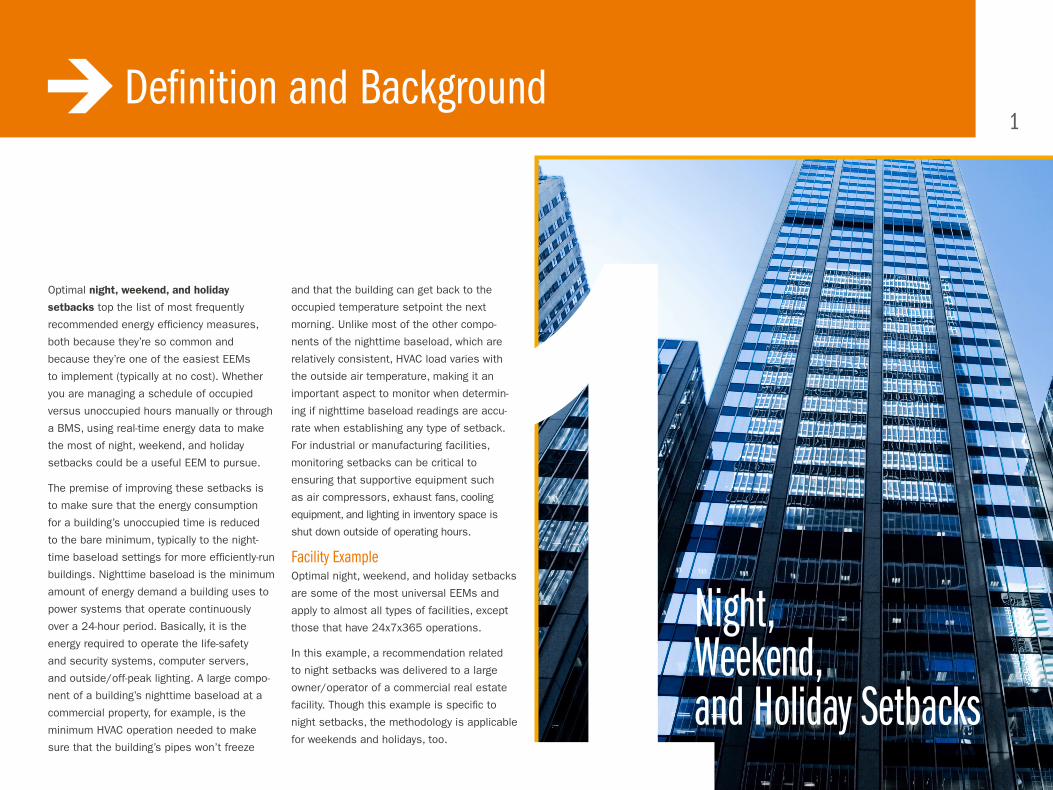
Optimal night, weekend, and holiday

setbacks top the list of most frequently

recommended energy efficiency measures,

both because they’re so common and

because they’re one of the easiest EEMs

to implement (typically at no cost). Whether

you are managing a schedule of occupied

versus unoccupied hours manually or through

a BMS, using real-time energy data to make

the most of night, weekend, and holiday

setbacks could be a useful EEM to pursue.

The premise of improving these setbacks is

to make sure that the energy consumption

for a building’s unoccupied time is reduced

to the bare minimum, typically to the night-

time baseload settings for more efficiently-run

buildings. Nighttime baseload is the minimum

amount of energy demand a building uses to

power systems that operate continuously

over a 24-hour period. Basically, it is the

energy required to operate the life-safety

and security systems, computer servers,

and outside/off-peak lighting. A large compo-

nent of a building’s nighttime baseload at a

commercial property, for example, is the

minimum HVAC operation needed to make

sure that the building’s pipes won’t freeze

and that the building can get back to the

occupied temperature setpoint the next

morning. Unlike most of the other compo-

nents of the nighttime baseload, which are

relatively consistent, HVAC load varies with

the outside air temperature, making it an

important aspect to monitor when determin-

ing if nighttime baseload readings are accu-

rate when establishing any type of setback.

For industrial or manufacturing facilities,

monitoring setbacks can be critical to

ensuring that supportive equipment such

as air compressors, exhaust fans, cooling

equipment, and lighting in inventory space is

shut down outside of operating hours.

Facility ExampleOptimal night, weekend, and holiday setbacks

are some of the most universal EEMs and

apply to almost all types of facilities, except

those that have 24x7x365 operations.

In this example, a recommendation related

to night setbacks was delivered to a large

owner/operator of a commercial real estate

facility. Though this example is specific to

night setbacks, the methodology is applicable

for weekends and holidays, too.

Definition and Background1

1

Challenge: Variable nighttime energy use during night setback

To check the efficacy of setbacks, analysts

usually track the nighttime baseload by

measuring a building’s energy demand after

all the occupants leave the building and

before the building starts up in the morning.

Baseloads for night setbacks should be

relatively consistent throughout a season.

Typically, any drastic changes in the baseload

represent some sort of inefficiency in the

building, such as overridden temperature

controls, accidentally disabled setback

controls, or malfunctioning equipment.

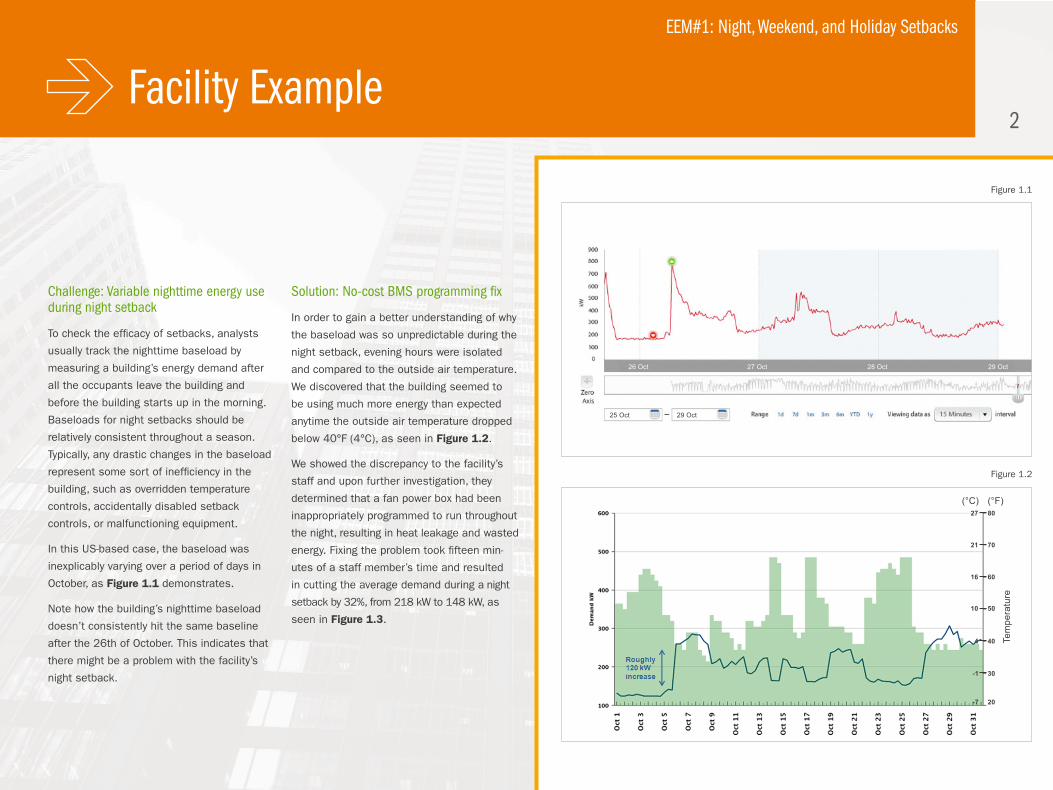
In this US-based case, the baseload was

inexplicably varying over a period of days in

October, as Figure 1.1 demonstrates.

Note how the building’s nighttime baseload

doesn’t consistently hit the same baseline

after the 26th of October. This indicates that

there might be a problem with the facility’s

night setback.

Solution: No-cost BMS programming fix

In order to gain a better understanding of why

the baseload was so unpredictable during the

night setback, evening hours were isolated

and compared to the outside air temperature.

We discovered that the building seemed to

be using much more energy than expected

anytime the outside air temperature dropped

below 40°F (4°C), as seen in Figure 1.2.

We showed the discrepancy to the facility’s

staff and upon further investigation, they

determined that a fan power box had been

inappropriately programmed to run throughout

the night, resulting in heat leakage and wasted

energy. Fixing the problem took fifteen min-

utes of a staff member’s time and resulted

in cutting the average demand during a night

setback by 32%, from 218 kW to 148 kW, as

seen in Figure 1.3.

2

Figure 1.1

Figure 1.2

EEM#1: Night, Weekend, and Holiday Setbacks

Facility Example

26 Oct 27 Oct 28 Oct 29 Oct

25 Oct 29 Oct

Tem

pera

ture

(°F)(°C)27

21

16

10

4

-1

-7

80

70

60

50

40

30

20

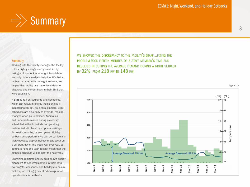
SummaryWorking with the facility manager, the facility

cut its nightly energy use by one-third by

taking a closer look at energy interval data.

Not only did our analysts help identify that a

problem existed with the night setback, we

helped this facility use meter-level data to

diagnose and correct bugs in their BMS that

were causing it.

A BMS is run on setpoints and schedules,

which can result in energy inefficiencies if

inappropriately set, as in this example. BMS

schedules are also easy to override, making

changes often go unnoticed. Anomalies

and underperformance during previously

scheduled setback periods can go along

undetected with less than optimal settings

for weeks, months, or even years. Holiday

setback underperformance can be particularly

tricky because a given holiday might occur on

a different day of the week year-over-year, so

getting it right one year doesn’t mean that the

setback schedule will be right the next year.

Examining real-time energy data allows energy

managers to see irregularities in their data

over nights, weekends, and holidays to ensure

that they are taking greatest advantage of all

opportunities for setbacks.

3

Figure 1.3

we showed the discrepancy to the facility’s staff...fixing the problem took fifteen minutes of a staff member’s time and resulted in cutting the average demand during a night setback by 32%, from 218 kw to 148 kw.

EEM#1: Night, Weekend, and Holiday Setbacks

Summary

Tem

pera

ture

(°F)(°C)27

21

16

10

4

-1

-7

80

70

60

50

40

30

20

Definition and Background4

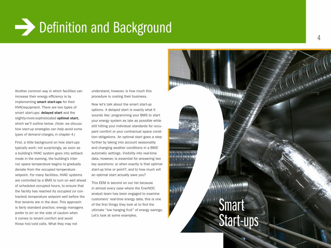
2Another common way in which facilities can

increase their energy efficiency is by

implementing smart start-ups for their

HVACequipment. There are two types of

smart start-ups: delayed start and the

slightly-more-sophisticated optimal start,

which we’ll outline below. (Note: we discuss

how start-up strategies can help avoid some

types of demand charges, in chapter 4.)

First, a little background on how start-ups

typically work: not surprisingly, as soon as

a building’s HVAC system goes into setback

mode in the evening, the building’s inter-

nal space temperature begins to gradually

deviate from the occupied temperature

setpoint. For many facilities, HVAC systems

are controlled by a BMS to turn on well ahead

of scheduled occupied hours, to ensure that

the facility has reached its occupied (or con-

tracted) temperature setpoint well before the

first tenants are in the door. This approach

is fairly standard practice; energy managers

prefer to err on the side of caution when

it comes to tenant comfort and avoid

those hot/cold calls. What they may not

understand, however, is how much this

procedure is costing their business.

Now let’s talk about the smart start-up

options. A delayed start is exactly what it

sounds like: programming your BMS to start

your energy system as late as possible while

still hitting your individual standards for occu-

pant comfort or your contractual space condi-

tion obligations. An optimal start goes a step

further by taking into account seasonality

and changing weather conditions in a BMS’

automatic settings. Visibility into real-time

data, however, is essential for answering two

key questions: a) when exactly is that optimal

start-up time or point?, and b) how much will

an optimal start actually save you?

This EEM is second on our list because

in almost every case where the EnerNOC

analyst team has been engaged to examine

customers’ real-time energy data, this is one

of the first things they look at to find the

ultimate “low hanging fruit” of energy savings.

Let’s look at some examples.

SmartStart-ups

Smart Start-up Type 1: Delayed Start

Facility ExampleA delayed start is applicable for most facilities

with conditioned spaces–office buildings,

hospitals, schools, government buildings, etc.

(Even most industrial/manufacturing facilities

have some conditioned office space, so it is

applicable there, too, though it is unlikely that

it could impact a significant percentage of

overall energy spend.) The facility discussed

in the following example is a conditioned

space facility.

Challenge: Wasting energy during building start-up

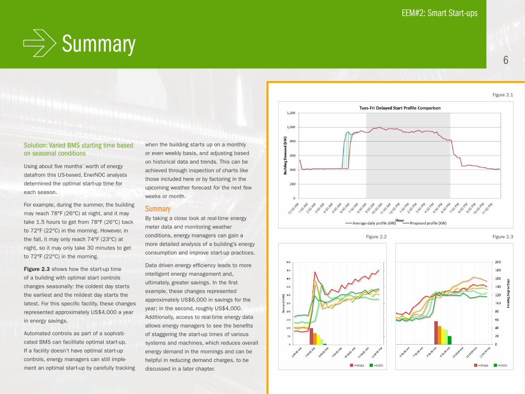
By examining one full month of data,

EnerNOC analysts generated the report

in Figure 2.1 for a conditioned space facility

in the US to improve the efficiency of the

building start-up. The shaded grey region

is the tenant occupancy period. The blue

line represents existing demand and the

red line is the proposed demand. The

shaded green region is the estimated

kWh savings potential.

We can see from this report that while

the building is starting up at 5:00a.m., its

contracted occupancy period doesn’t begin

until 8:00a.m. It’s likely that the building

doesn’t need a full three hours to reach the

desired setpoint, so it’s a good candidate for

a delayed start-up.

Solution: Incremental delayed building start-up

Most conditioned spaces have specific

schedules programmed into their BMS.

These systems are designed to make sure

that the lights are on and the building is

heated or cooled during scheduled hours.

To close the three-hour gap highlighted in

this facility example, we recommended

gradually moving the start-up time of the

BMS in the mornings back in 15-minute

increments daily to see how the building

responds, with the goal of finding the least

amount of time required to achieve the

desired setpoint. This measured approach

resulted in approximately US$6,000 in

savings for the year and ensured no adverse

impact to occupant comfort.

If your building doesn’t have a BMS, a smart

start-up strategy can be employed by adjusting

your HVAC start time and walking around your

facility and manually taking temperature

readings. You should adjust your HVAC start

times in small intervals daily (try 15 minutes

at first) until you find the right start-up time

that meets your building’s needs, keeping

your peak demand window in mind.

This analysis can be run for every building in

a portfolio to see where a delayed start-up

could be most beneficial for each building.

The analysis should be rerun at least three

times a year–summer, winter, and during

shoulder seasons (spring/fall)–to ensure

that a delayed start makes sense for each

season. We discuss more about seasonal

variation with optimal starts below.

Smart Start-up Type 2: Optimal Start

Facility ExampleAn optimal start is a more sophisticated

approach to conserving energy during a

building’s morning start-up. As such, an

optimal start-up is ideal for medium or large

commercial real estate facilities, particularly

those with hands-on facilities managers and

a more advanced BMS. The example below

highlights a commercial real estate facility

with a sophisticated BMS.

Challenge: Building start-up energy requirements vary by season

Throughout the year, weather conditions vary

and, as a result, so do the thermal losses

and gains a building experiences overnight

and in the morning. A very obvious example

of this is when a building achieves a very

different internal temperature overnight during

the winter versus the summer.

Figure 2.2 is one facility’s start-up profile

before implementing an optimal start-up.

The lines represent demand (kW), while the

bars represent the number of cooling degree

days or heating degree days (HDD/CDD).

Notice how the building starts up at roughly

the same time, despite changing weather

conditions. This graph suggests that the facility

is likely wasting energy in the mornings by

not differentiating the building start-up time

by season and changing weather conditions.

Since this facility has a sophisticated BMS,

they are a good candidate for an optimal start.

Facility Example5

EEM#2: Smart Start-ups

Summary6

Figure 2.2 Figure 2.3

EEM#2: Smart Start-ups

Figure 2.1

=max =min=max =min

Solution: Varied BMS starting time based on seasonal conditions

Using about five months’ worth of energy

datafrom this US-based, EnerNOC analysts

determined the optimal start-up time for

each season.

For example, during the summer, the building

may reach 78°F (26°C) at night, and it may

take 1.5 hours to get from 78°F (26°C) back

to 72°F (22°C) in the morning. However, in

the fall, it may only reach 74°F (23°C) at

night, so it may only take 30 minutes to get

to 72°F (22°C) in the morning.

Figure 2.3 shows how the start-up time

of a building with optimal start controls

changes seasonally: the coldest day starts

the earliest and the mildest day starts the

latest. For this specific facility, these changes

represented approximately US$4,000 a year

in energy savings.

Automated controls as part of a sophisti-

cated BMS can facilitate optimal start-up.

If a facility doesn’t have optimal start-up

controls, energy managers can still imple-

ment an optimal start-up by carefully tracking

when the building starts up on a monthly

or even weekly basis, and adjusting based

on historical data and trends. This can be

achieved through inspection of charts like

those included here or by factoring in the

upcoming weather forecast for the next few

weeks or month.

SummaryBy taking a close look at real-time energy

meter data and monitoring weather

conditions, energy managers can gain a

more detailed analysis of a building’s energy

consumption and improve start-up practices.

Data driven energy efficiency leads to more

intelligent energy management and,

ultimately, greater savings. In the first

example, these changes represented

approximately US$6,000 in savings for the

year; in the second, roughly US$4,000.

Additionally, access to real-time energy data

allows energy managers to see the benefits

of staggering the start-up times of various

systems and machines, which reduces overall

energy demand in the mornings and can be

helpful in reducing demand charges, to be

discussed in a later chapter.

12:00

AM

1:00 A

M2:0

0 AM

3:00 A

M4:0

0 AM

5:00 A

M6:0

0 AM

7:00 A

M8:0

0 AM

9:00 A

M10

:00 A

M11

:00 A

M12

:00 P

M1:0

0 PM

2:00 P

M3:0

0 PM

4:00 P

M5:0

0 PM

6:00 P

M7:0

0 PM

8:00 P

M9:0

0 PM

10:00

PM

11:00

PM

Definition and Background7

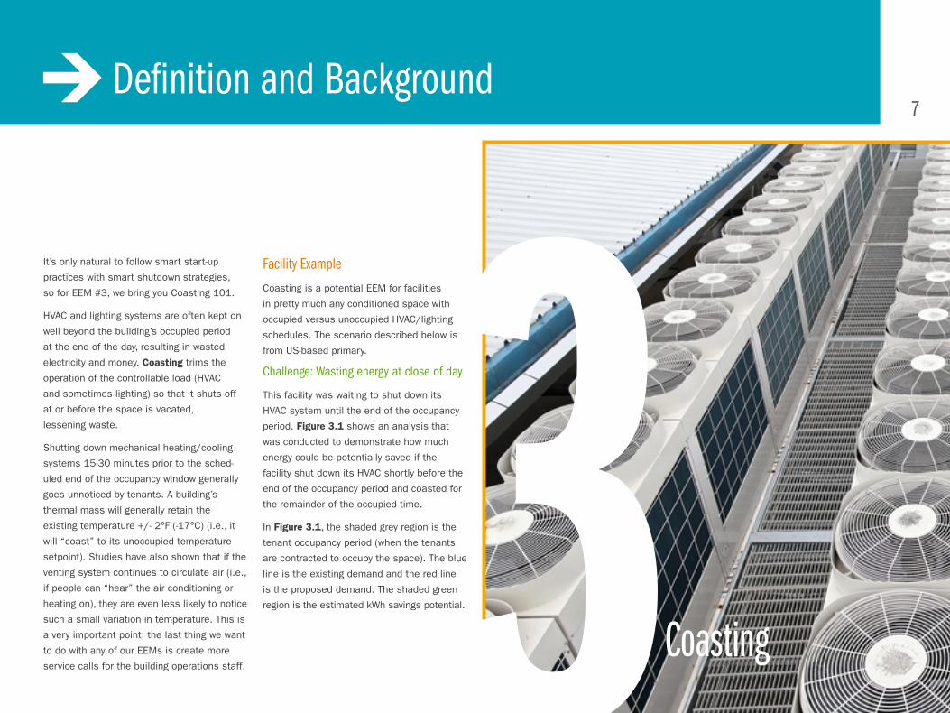
Coasting3It’s only natural to follow smart start-up

practices with smart shutdown strategies,

so for EEM #3, we bring you Coasting 101.

HVAC and lighting systems are often kept on

well beyond the building’s occupied period

at the end of the day, resulting in wasted

electricity and money. Coasting trims the

operation of the controllable load (HVAC

and sometimes lighting) so that it shuts off

at or before the space is vacated,

lessening waste.

Shutting down mechanical heating/cooling

systems 15-30 minutes prior to the sched-

uled end of the occupancy window generally

goes unnoticed by tenants. A building’s

thermal mass will generally retain the

existing temperature +/- 2°F (-17°C) (i.e., it

will “coast” to its unoccupied temperature

setpoint). Studies have also shown that if the

venting system continues to circulate air (i.e.,

if people can “hear” the air conditioning or

heating on), they are even less likely to notice

such a small variation in temperature. This is

a very important point; the last thing we want

to do with any of our EEMs is create more

service calls for the building operations staff.

Facility Example

Coasting is a potential EEM for facilities

in pretty much any conditioned space with

occupied versus unoccupied HVAC/lighting

schedules. The scenario described below is

from US-based primary.

Challenge: Wasting energy at close of day

This facility was waiting to shut down its

HVAC system until the end of the occupancy

period. Figure 3.1 shows an analysis that

was conducted to demonstrate how much

energy could be potentially saved if the

facility shut down its HVAC shortly before the

end of the occupancy period and coasted for

the remainder of the occupied time.

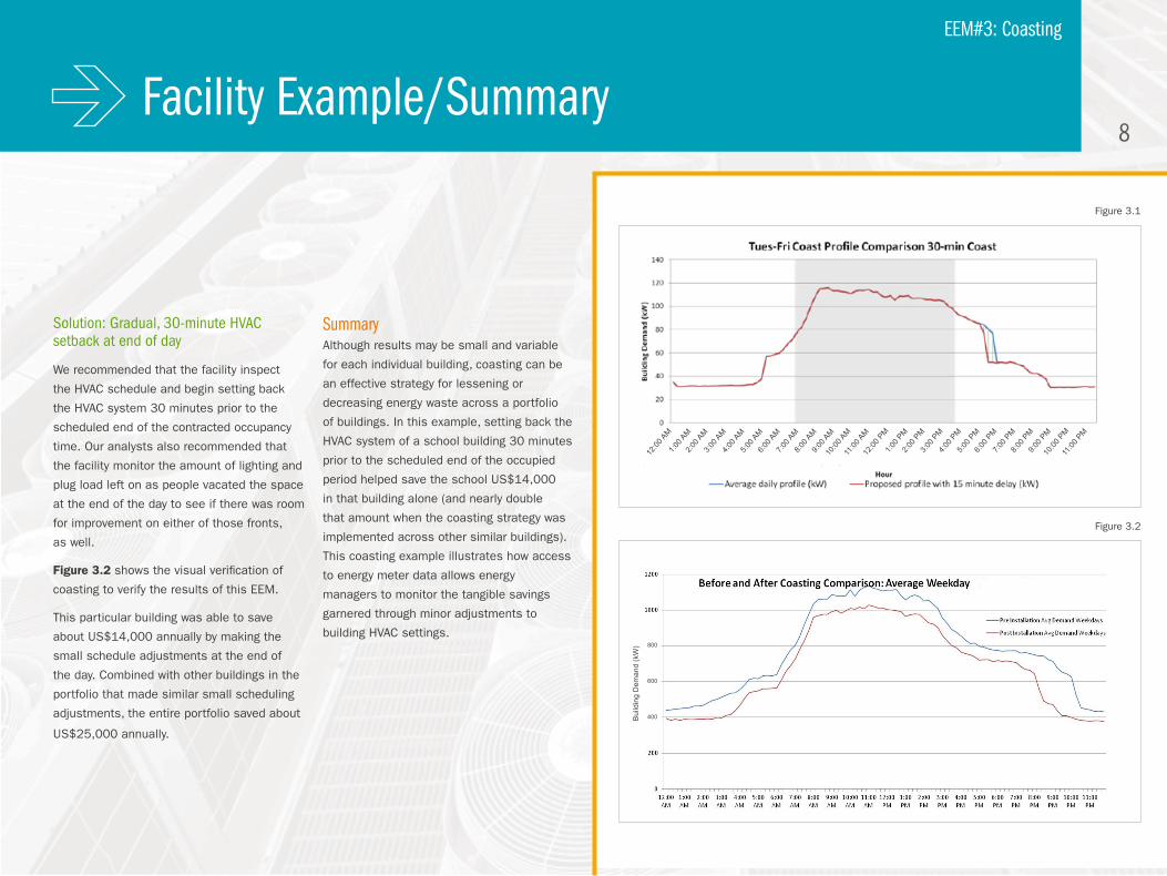
In Figure 3.1, the shaded grey region is the

tenant occupancy period (when the tenants

are contracted to occupy the space). The blue

line is the existing demand and the red line

is the proposed demand. The shaded green

region is the estimated kWh savings potential.

Facility Example/Summary8

Solution: Gradual, 30-minute HVAC setback at end of day

We recommended that the facility inspect

the HVAC schedule and begin setting back

the HVAC system 30 minutes prior to the

scheduled end of the contracted occupancy

time. Our analysts also recommended that

the facility monitor the amount of lighting and

plug load left on as people vacated the space

at the end of the day to see if there was room

for improvement on either of those fronts,

as well.

Figure 3.2 shows the visual verification of

coasting to verify the results of this EEM.

This particular building was able to save

about US$14,000 annually by making the

small schedule adjustments at the end of

the day. Combined with other buildings in the

portfolio that made similar small scheduling

adjustments, the entire portfolio saved about

US$25,000 annually.

SummaryAlthough results may be small and variable

for each individual building, coasting can be

an effective strategy for lessening or

decreasing energy waste across a portfolio

of buildings. In this example, setting back the

HVAC system of a school building 30 minutes

prior to the scheduled end of the occupied

period helped save the school US$14,000

in that building alone (and nearly double

that amount when the coasting strategy was

implemented across other similar buildings).

This coasting example illustrates how access

to energy meter data allows energy

managers to monitor the tangible savings

garnered through minor adjustments to

building HVAC settings.

Figure 3.1

Figure 3.2

EEM#3: Coasting

12:00

AM

1:00 A

M2:0

0 AM

3:00 A

M4:0

0 AM

5:00 A

M6:0

0 AM

7:00 A

M8:0

0 AM

9:00 A

M10

:00 A

M11

:00 A

M12

:00 P

M1:0

0 PM

2:00 P

M3:0

0 PM

4:00 P

M5:0

0 PM

6:00 P

M7:0

0 PM

8:00 P

M9:0

0 PM

10:00

PM

11:00

PM

Bui

ldin

g D

eman

d (k

W) 800

600

400

Definition and Background9

4Demand charge management may be fourth

on this list, but it is often ranked #1 as a

savings opportunity, depending on a) how

you’re billed for electricity, and b) how much

electricity your facility consumes at critical

times. There are different kinds of demand

charges, like Transmission System Use of

Network (TSUoN) charges, Time of Use (ToU)

tariffs, and individual facility peak demand

charges. The severity of the demand charge

can vary, with facility peak demand charges

- which are common in the US - sometimes

accounting for 30% of a total energy bill.

What is a peak demand charge?

In many cases, electricity use is metered

(and you are charged) in two ways: first,

based on your building’s total consumption

in a given month (kWh), and second, on your

building’s demand (kW), based on the highest

rate of consumption of your building during

the given billing period (typically a 15-minute

interval during that billing cycle).

To use an analogy, think about consumption

(kWh) as the number that registers on your

car’s odometer (how far you’ve driven), and

demand (kW) as what is captured on your

speedometer at the moment when you hit

your max speed. Consumption is your overall

electricity use, and demand is your peak

intensity, or maximum “speed.”

With residential buildings, these two charges

may appear as a combined charge (like all

tariffs, this varies), but because commer-

cial and industrial users have significant

variance in both consumption and demand,

these charges are often (but not always)

broken out. National Grid in the US explains:

“Some [commercial and industrial energy

users] need large amounts of electricity once

in awhile–others, almost constantly.” And

because electricity can’t be stored, meeting

these customers’ needs quickly becomes

complex and costly, requiring “a vast array

of expensive equipment–transformers,

wires, substations, and generating stations–

on constant standby. In some areas, all

customers are assessed a demand charge

to cover these costs, while in others, cus-

tomers who create this exceptionally high,

or “peak,” demand are then correspondingly

charged more for it.

Demand Charge Management

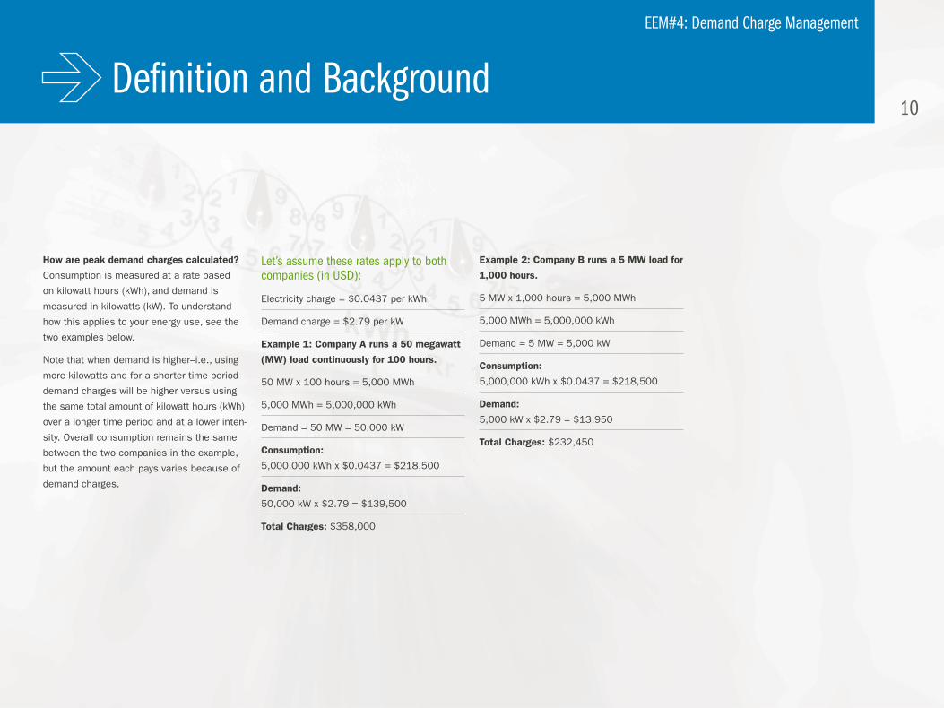
How are peak demand charges calculated?

Consumption is measured at a rate based

on kilowatt hours (kWh), and demand is

measured in kilowatts (kW). To understand

how this applies to your energy use, see the

two examples below.

Note that when demand is higher–i.e., using

more kilowatts and for a shorter time period–

demand charges will be higher versus using

the same total amount of kilowatt hours (kWh)

over a longer time period and at a lower inten-

sity. Overall consumption remains the same

between the two companies in the example,

but the amount each pays varies because of

demand charges.

Let’s assume these rates apply to both companies (in USD):

Electricity charge = $0.0437 per kWh

Demand charge = $2.79 per kW

Example 1: Company A runs a 50 megawatt

(MW) load continuously for 100 hours.

50 MW x 100 hours = 5,000 MWh

5,000 MWh = 5,000,000 kWh

Demand = 50 MW = 50,000 kW

Consumption:

5,000,000 kWh x $0.0437 = $218,500

Demand:

50,000 kW x $2.79 = $139,500

Total Charges: $358,000

Example 2: Company B runs a 5 MW load for

1,000 hours.

5 MW x 1,000 hours = 5,000 MWh

5,000 MWh = 5,000,000 kWh

Demand = 5 MW = 5,000 kW

Consumption:

5,000,000 kWh x $0.0437 = $218,500

Demand:

5,000 kW x $2.79 = $13,950

Total Charges: $232,450

Definition and Background10

EEM#4: Demand Charge Management

Definition and Background

Figure 4.1

using real-time energy data monitoring, we were able to see that the facility’s cleaning schedule was causing a spike in the facility’s peak demand charge. the crew was instructed to move the clean-ing schedule to outside the peak demand window, which lowered the facility’s…peak demand charge by approximately us$45,000 annually.

EEM#4: Demand Charge Management

11

For the same amount of kilowatt hours

used–i.e., at the same consumption level,

albeit at different intensities–Company A pays

significantly more in charges.

Depending on your rate structure, peak

demand charges can represent up to 30%

of your utility bill. Certain industries, like

manufacturing and heavy industrials, typically

experience much higher peaks in demand

due largely to the start-up of energy-intensive

equipment, making it even more imperative to

find ways to reduce this charge.

Facility Example/Summary

Regardless of your industry, taking steps to

reduce demand charges will save money.

Let’s take a look at how one US-based facility

boosted their bottom line by adjusting their

peak demand charges using real-time energy

data monitoring.

Facility ExampleWhether or not building scheduling and peak

demand management can help a facility cut

their energy bill depends largely on the build-

ing’s energy use patterns and the specific

rate structure offered by the utility. In the

case highlighted in this example, an industrial

facility had a steam turbine generator that

generated electricity for the facility.

Challenge: On-peak demand charges

Building owners often tweak their equipment

scheduling to balance the trade off between

consumption and demand charges. In this

particular example, the crew had to bring

the boiler (that supplied the steam for the

facility’s turbine) offline to clean it every night.

While cleaning the boiler, peak demand shot

up 400-500 kW each night, as illustrated

in Figure 4.1.

Upon reviewing the facility’s energy data,

analysts found that peak demand charges

were much higher than necessary because

the cleaning was scheduled to occur within

the facility’s peak demand window, the

on-peak hours during which peak demand

charges are most expensive. This problem

appeared to be a prime candidate for peak

demand management.

Solution: No-cost scheduling adjustment

Using real-time energy data monitoring, we

were able to see that the facility’s cleaning

schedule was causing a spike in the facil-

ity’s peak demand charge. The crew was

instructed to move the cleaning schedule to

outside the peak demand window, which low-

ered the facility’s demand during the on-peak

hours, and thus lowered its peak demand

charge by approximately US$45,000 annually.

SummaryVisibility into real-time energy data allowed

this facility to better its consumption pattern

and peak demand charges. By making a

no-cost scheduling adjustment, they were

able to lower their peak demand charge by

US$45,000 annually.

Energy managers can manage peak demand

charges by using real-time energy data to

monitor and adjust when they achieve their

peak demand–and also lowering the peak

demand actually reached during a billing

cycle. Some other examples of peak

demand management include starting up

the building’s systems before on-peak hours

or operating the most energy intensive

equipment at different times so all machines

aren’t running simultaneously, which makes

peak demand lower.

EEM#4: Demand Charge Management

12

Definition and Background13

5Economizing is when a facility’s HVAC system

uses outside air conditions to help condition

the building. One way to do this is by using

dampers that are designed to allow “free

cooling” with outside air. When the outside

air is cooler than the return air, the outside

air dampers are opened completely. When the

outside air is warmer than the return air, the

outside air dampers are closed.

This EEM is likely to occur when outside

temperatures are between 50°F (10°C) and

65°F (18°C), but that can vary depending

on facility construction and location.

See the example below to learn how we

used real-time energy data to take full

advantage of outside air conditions to

save energy and money.

Facility ExampleEconomizing is applicable for most condi-

tioned spaces. Sophisticated BMS systems

have this functionality built into them, and

therefore are good candidates for reviewing

the sequencing of the system and the

system’s setpoints. It’s common to find

a BMS that has deviated from its original

setpoints after gradual adjustments and

thus its economizing capabilities have been

impacted. This example highlights a commer-

cial real estate facility.

Challenge: Not using outside air to de-crease energy needed to condition space

The US-based facility in this example appears

to switch from heating to cooling its condi-

tioned space at 55°F (13°C) (called their

change point), as Figure 5.1 illustrates.

Since the building switches from cooling to

heating at approximately one temperature,

it’s apparent that this facility is not taking

advantage of optimal weather conditions

between 45°F (7°C) and 60°F (16°C). If

the facility was economizing properly, the

occupied period should reflect a relatively

flat line during that temperature bandwidth,

indicating that less energy is being used to

condition the space as compared to either

the heating or cooling period. Economizing

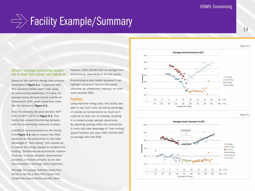
Solution: Leverage economizing capabili-ties to allow “free cooling” with outside air

Based on the real-time energy data analysis

illustrated in Figure 5.1, it appeared that

this US-based facility wasn’t fully using

its economizing capabilities. If it were, its

average hourly demand versus outside air

temperature (OAT) graph would look more

like the demand in Figure 5.2.

Note the relatively flat area between 40°F

(4°C) to 60°F (16°C) in Figure 5.2. This

facility has properly functioning dampers

and has economizing measures in place.

EnerNOC’s recommendation to the facility

from Figure 5.1 was to inspect the HVAC

setpoints for the economizer to fully take

advantage of “free cooling” with outside air

to reduce the energy needed to condition the

building. Sometimes the economizer malfunc-

tions due to stuck dampers, disconnected

actuators, or broken sensors, so we also

recommended a thorough parts inspection.

Although the savings potential varies from

facility to facility, a 300,000 square foot

conditioned space facility typically saves

between US$1,000-$4,000 on average from

economizing, depending on its fuel source.

Economizing is also helpful because it can

highlight equipment failures that would

otherwise go undetected, making it an even

more valuable EEM.

SummaryUsing real-time energy data, this facility was

able to see that it was not taking advantage

of outside air temperatures as much as it

could be to help cool its building, resulting

in a missed energy savings opportunity.

By adjusting settings within the economizer

to more fully take advantage of “free cooling,”

typical facilities can save US$1,000-$4,000

on average from this EEM.

Facility Example/Summary

Figure 5.1

Figure 5.2

EEM#5: Economizing

14

Outside Air Temp 10 20 30 40 50 60 70 80 90 100 (°F)

-12 -7 -1 4 10 16 21 27 32 38 (°C)

Outside Air Temp 10 20 30 40 50 60 70 80 90 100 (°F)

-12 -7 -1 4 10 16 21 27 32 38 (°C)

Low and no-cost energy efficiency measures

are a great way to either get started with

energy management, or to take your current

efforts to the next level. Having access to

real-time energy meter data is instrumental

in identifying numerous EEMs, including those

outlined in this eBook, as well as others.

Without interval energy data, energy managers

have to rely on sometimes months-old data

from their utility bills without visibility into daily

operations and energy use to try and track

down potential inefficiencies and anomalies.

We also acknowledge that you have limited

time to pore through all of this data and

manually conduct analyses, which is why

EnerNOC’s energy intelligence software

(EIS) provides visibility into how energy is

consumed and where it is being wasted,

and provides the tools – including powerful

analytics, reports, and dashboards – to help

you identify priority action. When that doesn’t

go far enough, our professional services team

can dig into your energy data to spot these

and other energy efficiency opportunities and

deliver them to you in a ranked list by ROI.

For more information, visit our website

at www.enernoc.com or contact a member

of our team.

If you’re interested in even more tips, tricks,

and energy management best practices, check

out our EnergySMART Blog to take your

energy efficiency management knowledge

to the next level.

Conclusion15

About EnerNOCEnerNOC, Inc. is a leading provider of energy intelligence software (EIS). EnerNOC unlocks the full value of energy management for thousands of customers worldwide by delivering a comprehensive suite of software applications and professional services that help users buy energy better, manage utility bills, reduce energy consumption, participate in demand response, and manage peak demand.

For more information, visit www.enernoc.com. Catch up on the latest best practices in energy management on our EnergySMART blog, energysmart.enernoc.com.

P14048 © EnerNOC, Inc. All rights reserved.

About the Author16