Non-Cumulative Resource AnalysisAuthor’s version∗∗

Elvira Albert1, Jesus Correas1, Guillermo Roman-Dıez2

1 DSIC, Complutense University of Madrid, Spain2 DLSIIS, Technical University of Madrid, Spain

Abstract. Existing cost analysis frameworks have been defined for cu-mulative resources which keep on increasing along the computation.Traditional cumulative resources are execution time, number of exe-cuted steps, amount of memory allocated, and energy consumption. Non-cumulative resources are acquired and (possibly) released along the exe-cution. Examples of non-cumulative cost are memory usage in the pres-ence of garbage collection, number of connections established that arelater closed, or resources requested to a virtual host which are releasedafter using them. We present, to the best of our knowledge, the firstgeneric static analysis framework to infer an upper bound on the peakcost for non-cumulative types of resources. Our analysis comprises sev-eral components: (1) a pre-analysis to infer when resources are beingused simultaneously, (2) a program-point resource analysis which infersan upper bound on the cost at the points of interest (namely the pointswhere resources are acquired) and (3) the elimination from the upperbounds obtained in (2) of those resources accumulated that are not usedsimultaneously. We report on a prototype implementation of our analysisthat can be used on a simple imperative language.

1 Introduction

Cost analysis (a.k.a. resource analysis) aims at statically (without executing theprogram) inferring upper bounds on the resource consumption of the programas functions of the input data sizes. Traditional resources (e.g., time, steps,memory allocation, number of calls) are cumulative, i.e., they always increasealong the execution. Ideally, a cost analysis framework is generic on the typeof resource that the user wants to measure so that the resource of interest is aparameter of the analysis. Several generic cost analysis frameworks have beendefined for cumulative resources using different formalisms. In particular, theclassical framework based on recurrence relations has been used to define a cost

2 Appeared at Proc. 21st International Conference on Tools and Algorithms for theConstruction and Analysis of Systems (TACAS’15), London, UK, April 11-18, 2015.The final publication is available at http://link.springer.com/chapter/10.1007/978-3-662-46681-0_6

analysis for a Java-like language [?]; approaches based on program invariants aredefined in [?,?]; type systems have been presented in [?].

Non-cumulative resources are first acquired and then released. Typical exam-ples are memory usage in the presence of garbage collection, maximum numberof connections established simultaneously, the size of the stack of activationrecords, etc. The problem is nowadays also very relevant in virtualized systems,as in cloud computing, in which resources are acquired when needed and releasedafter being used. It is recognized that non-cumulative resources introduce newchallenges in resource analysis [?,?]. This is because the resource consumptioncan increase and decrease along the computation, and it is not enough to rea-son on the final state of the execution, but rather the upper bound on the costcan happen at any intermediate step. We use the term peak cost to denote suchmaximum cost of the program execution for non-cumulative resources.

While the problem of inferring the peak cost has been studied in the contextof memory usage for specific models of garbage collection [?,?,?], a generic frame-work to estimate the non-cumulative cost does not exist yet. The contributionof this paper is a generic resource analysis framework for a today’s imperativelanguage enriched with instructions to acquire and release resources. Thus, ourframework can be instantiated to measure any type of non-cumulative resourcethat is acquired and (optionally) freed. The analysis is defined in two steps whichare our main contributions: (1) We first infer the sets of resources which can bein use simultaneously (i.e., they have been both acquired and none of them re-leased at some point of the execution). This process is formalized as a staticanalysis that (over-)approximates the sets of acquire instructions that can bein use simultaneously, allowing us to capture the simultaneous use of resourcesin the execution. (2) We then perform a program-point resource analysis whichinfers an upper bound on the cost at the points of interest, namely the points atwhich the resources are acquired. From such upper bounds, we can obtain thepeak cost by just eliminating the cost due to acquire instructions that do nothappen simultaneously with the others (according to the analysis informationgathered at step 1). Additionally, we describe an extension of the frameworkwhich can improve the accuracy of the upper bounds by accounting only oncethe cost introduced at program points where resources are allocated and re-leased repeatedly. Finally, we illustrate how the framework can be extended toget upper bounds for programs that allocate different kinds of resources.

We demonstrate the accuracy and feasibility of our approach by implement-ing a prototype analyzer for a simple imperative language. Preliminary experi-ments show that the non-cumulative resource analysis achieves gains up to 92.9%(on average 53.9%) in comparison to a cumulative resource analysis. The analysiscan be used online from a web interface at http://costa.ls.fi.upm.es/noncu.

2 The Notion of Peak Cost

We start by defining the notion of peak cost that we aim at over-approximatingby means of static analysis in the concrete setting.

2

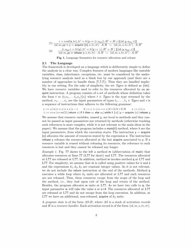
(1)r = eval(e, tv), tr′ = tr[y 7→ 〈r, app〉], H ′ = H ∪ {|〈id, y, app, r〉|}

〈id,m, pp ≡ y = acquire (e); s, tv, tr〉 ·A;H ; 〈id,m, s, tv, tr′〉 ·A;H ′

(2)〈r, app′〉 = tr(y), tr′ = tr[y 7→ ⊥], H ′ = H \ {|〈id, y, app′ , r〉|}

〈id,m, pp ≡ release y; s, tv, tr〉 ·A;H ; 〈id,m, s, tv, tr′〉 ·A;H ′

Fig. 1. Language Semantics for resource allocation and release

2.1 The LanguageThe framework is developed on a language which is deliberately simple to definethe analysis in a clear way. Complex features of modern languages like mutablevariables, class, inheritance, exceptions, etc. must be considered by the under-lying resource analysis used as a black box by our approach (and there are anumber of approaches to handle them [?,?,?]). Thus they are handled implic-itly in our setting. For the sake of simplicity, the set Types is defined as {int}.We have resource variables used to refer to the resources allocated by an ac-quire instruction. A program consists of a set of methods whose definition takesthe form t m (t1v1, . . . tnvn){s} where t ∈ Types is the type returned by themethod, v1, . . . , vn are the input parameters of types t1, . . . , tn ∈ Types and s isa sequence of instructions that adheres to the following grammar:

e ::= x |n | e+ e | e ∗ e | e− e b ::= e > e | e == e | b ∧ b | b ∨ b | !b s ::= i | i; si ::= x=e |x=m(z) | return x | if b then s1 else s2 |while b {s} | y = acquire (e) | release y

We assume that resource variables, named y, are local to methods and they can-not be passed as input parameters nor returned by methods (otherwise trackingsuch references is more complex, while it is not relevant to the main ideas in thepaper). We assume that the program includes a main(x) method, where x are theinput parameters, from which the execution starts. The instruction y = acquire(e) allocates the amount of resources stated by the expression e. The instructionrelease y releases the resources allocated at the last acquire associated to y. If aresource variable is reused without releasing its resources, the reference to suchresources is lost and they cannot be released any longer.

Example 1. Fig. ?? shows to the left a method m (abbreviation of main) thatallocates resources at lines ?? (L?? for short) and L??. The resources allocatedat L?? are released at L??. In addition, method m invokes method q at L?? andL??. For simplicity, we assume that m is called using positive values for n and sand the expressions k1, k2, k3 are constant integer values. As it is not relevant,we do not include the return instruction at the end of the methods. Method qexecutes a while loop where k2 units are allocated at L?? and such resourcesare not released. Thus, these resources escape from the scope of the loop andthe method, i.e., they leak upon exit of the loop and return of the method.Besides, the program allocates w units at L??. As we have two calls to q, theinput parameter w will take the value s or s+4. The resources allocated at L??are released at L?? and do not escape from the loop execution. In addition, atL?? we have an additional, non-released, acquire of k3 units.

A program state is of the form AS;H, where AS is a stack of activation recordsand H is a resource handler. Each activation record is of the form 〈id,m, s, tv, tr〉,

3

1 m (int n, int s){2 1© x=acquire(k1);3 q(n,s);4 2© y=acquire(s);5 release x;6 q(n+2, s+4);7 }8 q (int i , int w){9 while(i > 0) {

10 3© z=acquire(k2);11 4© r=acquire(w);12 release r ;13 i = i − 1;14 }15 5© t=acquire(k3);16 }

x:k1

L2

S1

z:k2

x:k1

L10

S2

r:s

z:k2

x:k1

L11

S3

z:k2

x:k1

L12

S4

z:k2

z:k2

x:k1

L10

S5

r:s

z:k2

z:k2

x:k1

L11

S6

z:k2

z:k2

x:k1

L12

S7

. . .

r:s

z:k2

:nz:k2

x:k1

L11

S8

t:k3

z:k2

:nz:k2

x:k1

L15

S9

t:k3

zn:k2 n times

x:k1

L16

S10

t:k3

zn:k2

x:k1

L4

S11

y:s

t:k3

zn:k2

x:k1x:k1

L4

S12

y:s

t:k3

zn:k2

L5

S13

z:k2

y:s

t:k3

zn:k2

L10

S14

r:s+4

z:k2

y:s

t:k3

zn:k2

L11

S15

. . .

r:s+4

z:k2

:n+2

z:k2

y:s

t:k3

zn:k2

L11

S16

z:k2

:n+2

z:k2

y:s

t:k3

zn:k2

L14

S17

t:k3

z:k2

:n+2

z:k2

y:s

t:k3

zn:k2

L13

S18

n + 2

Fig. 2. Running Example

where id is a unique identifier, m is the name of the method, s is the sequenceof instructions to be executed, tv is a variable mapping and tr is a resourcevariable mapping. When resources are allocated in m, tr maps the correspond-ing resource variable to a tuple of the form 〈r, app〉, where r is the amount ofresources allocated and app is the program point of the instruction where the re-sources have been allocated. The resource handler H is a multiset which storesthe resources allocated so far, containing elements of the form 〈id, y, app, r〉,where id is the activation record identifier, y is the variable name, app is theprogram point of the acquire and r is the amount of resources allocated. Fig. ??shows, in a rewriting-based style, the rules that are relevant for the resource con-sumption. The semantics of the remaining instructions is standard. Intuitively,rule (1) evaluates the expression e and adds a new element to H. As H storesthe resources allocated so far, it might contain identical tuples. Moreover, theresource variable mapping tr is updated with variable y linked to 〈r, app〉. Rule(2) takes the information stored in tr for y, i.e. 〈r, app〉, and removes from Hone instance of the corresponding element. In addition, variable y is updated topoint to ⊥, which means that y does not have any resources associated. Whenthe execution performs a release on a variable that maps to ⊥ (because no ac-quire has been performed or because it has already been released), the resourcesstate is not modified. Execution starts from a main method and an initial stateS0 = 〈0,main, body(main), tv(x), ∅〉; ∅, where tv(x) is the variable mapping ini-tialized with the values of the input parameters. Complete executions are of theform S0 ; S1 ; . . .; Sn where Sn corresponds to the last state. Infinite tracescorrespond to non-terminating executions.

Example 2. To the right of Fig. ?? we depict the evolution of the resourcesaccumulated in H. We use Si, to refer to the execution state i and, below eachstate, we include the program line which is executed at such state. For eachstate we show the elements stored in H but, for simplicity, we do not include

4

in the figure the id nor app. At S1, H accumulates k1 units due to the acquireat L??. S2, S3 and S4 depict H along the first iteration of the loop, where k2units are acquired and not released from z. Moreover, within the loop, s unitsare acquired at L?? and released from r at L??. At S5, which corresponds to thesecond iteration of the loop, we reuse the resource variable z and we have twoidentical elements in H. As the loop iterates n times, at the last iteration (S9)we have (n−1)∗k1 units that have lost their reference. Additionally, k3 extraunits pointed by t are allocated at S9. At S10, which corresponds to the end ofthe execution of the method, n∗k2+k3 units escape from the first execution ofq and they are no longer available to be released. We represent such escapedresources with light grey color. For brevity, we use zn:k2 to represent n instancesof the element z:k2. At S12 we acquire s resources and we release the k1 unitspointed by x at S13. At S14 we start a new execution of method q.

2.2 Definition of Peak Cost

Let us formally define the notion of peak cost in the concrete setting. The peakcost corresponds to the maximum amount of resources that are used simultane-ously. We use Hi to refer to the multiset H at Si, and we use Ri to denote theamount of resources contained in Hi, i.e., Ri =

∑{r | 〈 , , , r〉 ∈ Hi}. By ’ ’, we

mean any possible value. In the next definition, we use Ri to define the notionof peak cost for an execution trace.

Definition 1 (concrete peak cost). The peak cost of an execution tracet≡S0;Sn of a program P on input values x is defined as P(x)=max({Ri | Si∈t}).

Example 3. According to the evolution of H shown to the right of Fig. ??, themaximum value of Ri could be reached at four different states, S8, S12, S16

and S18. We ignore those states where H is subsumed by other states as theycannot be maximal. For instance, states S1 to S7 or S9 are subsumed by S8;or S12 contains S10, S11 and S13. Thus, P(n, s)=max(R8, R12, R16, R18), whereR8 = k1+n∗k2+s, R12 = k1+n∗k2+k3+s, R16 = n∗k2+k3+s+(n+2)∗k2+(s+4), andR18=n∗k2+k3+s+(n+2)∗k2+k3. Thus, the peak cost of the example depends notonly on the input parameters n, s, but also on the values of k1, k2, k3.

3 Simultaneous Resource Analysis

The simultaneous resource analysis (SRA) is used to infer the sets of acquireinstructions that can be simultaneously in use. The abstract state of the SRAconsists of two sets C and H. The set C contains elements of the form y:app

indicating that the resource variable y is linked to the acquire instruction atprogram point pp. Since it is not always possible to relate the acquire instruc-tion to its corresponding resource variable, we use ?:app to represent that someresources have been acquired at app but the analysis has lost the variable linkedto app. The set H is a set of sets, such that each set contains those app that aresimultaneously alive in an abstract state of the analysis. Let us introduce somenotation. We use m to refer to the program point after the return instruction

5

(1) τ(pp : y=acquire( ), 〈C,H〉) = 〈C[y:app′/ ? :app′ ] ∪ {y:app},H ] {A(C) ∪ {app}}〉(2) τ(pp : release y, 〈C,H〉) = 〈C \ {y:app},H〉(3) τ(pp : m( ), 〈C,H〉) = 〈C ∪ Cm[x:app′/ ? :app′ ],H ] {A(C) ∪M | M ∈ Hm}〉(4) τ(pp : b, 〈C,H〉) = 〈C,H〉

Fig. 3. Transfer Function of the Simultaneous Resource Analysis

of method m. We use Cpp (resp. Hpp) to denote the value of C (resp. H) afterprocessing the instruction at program point pp. A(C) is the set {app | :app ∈ C}that contains all app in C. The operation H1 ] H2, where H1 and H2 are setsof sets, first applies H = H1 ∪ H2, and then removes those sets in H that arecontained in another set in H.

The analysis of each method m abstractly executes its instructions, by ap-plying the transfer function τ in Fig. ??, such that the abstract state at eachprogram point describes the status of all acquire instructions executed so far.The set C is used to infer the local effect of the acquire and release instructionswithin a method. The set H is used to accumulate the information of the ac-quire instructions that might have been in use simultaneously. Let us explainthe different cases of the transfer function τ . The execution of acquire, case (1),links the acquire to the resource variable y by adding {y:app} to C. As a resourcevariable can only point to one acquire instruction, in (1) we update any existingy:app′ by removing the previous link to y and replacing it by ?. In addition, rule(1) performs the operation {A(C) ∪ {app}} ] H to capture in H the acquiredresources simultaneously in use at this point. In (2) we remove the last acquireinstruction pointed to by the resource variable y. When a method is invoked (rule(3)), we add to C those resources that might escape from m (Cm) but replacingtheir resource variables in m by ? (as resource variables are local). Additionally,at (3), all sets in Hm are joined with A(C) to capture the resources that mighthave been simultaneously alive in the execution of m. The resulting sets of suchoperation are added to H. We define the t operation between two abstract states〈C1,H1〉 t 〈C2,H2〉 as 〈C1 ∪ C2,H1 ]H2〉. The analysis of while loops requires it-erating until a fixpoint is reached. As the number of acquire instructions and thenumber of resource variables in the program are finite, widening is not needed.

Example 4. Let us apply the SRA to the running example. To avoid clutteringthe expressions, instead of the line numbers, we use ai to refer to the acquireat the program point marked with i© in Fig. ??. For instance, a1 refers to theacquire marked with 1© at L??. We use Cl (resp. Hl) to denote the set C (resp.H) at line l. Let us see the results of the SRA for some selected program points.

6

C2 = {x:a1} H2 = {{a1}}C3 = {x:a1, ?:a3, ?:a5} H3 = {{a1, a3, a4}, {a1, a3, a5}}C4 = {x:a1, ?:a3, ?:a5, y:a2} H4 = {{a1, a3, a4}, {a1, a3, a5, a2}}C5 = {?:a3, ?:a5, y:a2} H5 = {{a1, a3, a4}, {a1, a3, a5, a2}}C6 = Cm = {?:a3, ?:a5, y:a2} H6=Hm={{a1, a3, a4}, {a1, a3, a5, a2}, {a2, a3, a4, a5} *©}C10 = {?:a3, z:a3} H10 = {{a3, a4}}C11 = {?:a3, z:a3, r:a4} H11 = {{a3, a4}}C12 = C14 = {?:a3, z:a3} H12 = H14 = {{a3, a4}}C15 = Cq = {?:a3, z:a3, t:a5} H15 = Hq = {{a3, a4}, {a3, a5}}We can see that C11 is the only program point where a4 is alive as it is releasedat L??. On the contrary, as a3 is not released within the loop, we include ?:a3 inC10−C14, and it escapes from the loop and from q. AsH gathers all app that mightbe alive at any program point, when the fixpoint is reached, H10 −H14 containthe set {a3, a4}. The computation of Hq is done by means of the operationA(Cq)]H14, that is, Hq={{a3, a5}}] {{a3, a4}}={{a3, a5}, {a3, a4}}, capturingthat a3, a4, a5 are not simultaneously in use at any state of q. Moreover, we cansee in Cq that the resources allocated at a3 and a5 escape from the executionof q. Let us continue with the computation of C3 and H3. Firstly, ?:a3 and?:a5 are added to C3. Secondly, H3 is computed by adding C2={a1} to all setsin Hq. To compute C4, the analysis adds y:a2 to C3. The computation of H4

adds {a1, a3, a5, a2} to H3, and replaces {a1, a3, a5} because it is a subset of{a1, a3, a5, a2}. Finally, to obtain H6, the set A(C6)={a3, a5, a2} is added tothe sets in Hq, resulting in the set T = {{a2, a3, a4, a5}, {a2, a3, a5}}. Then H6

is obtained by computing H5 ] T . Note that {a2, a3, a5} is not in H6 as it iscontained in a set of H5.

Theorem 1 (soundness). Given an execution trace t ≡ S0; . . .;Sn of aprogram P on input values x, for any state Si ∈ t, we have that:

(a) ∃ H ∈ H ¨main. A(Hi) ⊆ H where A(Hi) = {app | 〈 , , app, 〉 ∈ Hi};(b) if ∃〈 , , app, 〉 ∈ Hn then :app ∈ C ¨main

4 Non-Cumulative Resource Analysis

In this section we present our approach to use the information obtained in Sec. ??to infer the peak cost of the execution. The first part, Sec. ??, consists in perform-ing a program-point resource analysis in which we are able to infer the resourcesacquired at the points of interest. In Sec. ??, we discard from the upper boundobtained before those resources which are not used simultaneously.

4.1 Program-Point Resource Analysis

Our goal is to distinguish within the upper bounds (UB) obtained by resourceanalysis the amount of resources acquired at a given program point. To do so, werely on the notion of cost center (CC) [?]. Originally, CCs were introduced forthe analysis of distributed systems, such that, each CC is a symbolic expressionof the form c(o) where o is a location identifier used to separate the cost ofeach distributed location. Essentially, the resource analysis assigns the cost of

7

an instruction inst to the distributed location o by multiplying the cost dueto the execution of the instruction, denoted cost(inst) in a generic way, by thecost center of the location c(o), i.e., cost(inst)∗c(o). This way, the UBs that theanalysis obtains are of the form

∑c(oi)∗Ci, where each oi is a location identifier

and Ci is the total cost accumulated at this location.Importantly, the notion of CC can be used in a more general way to define the

granularity of a cost analyzer, i.e., the kind of separation that we want to observein the UBs. In our concrete application, the expressions of the cost centers oiwill refer to the program points of interest. Thus, we are defining a resourceanalyzer that provides the resource consumption at program point level, i.e., aprogram point resource analysis. In particular, we define a CC for each acquireinstruction in the program. Thus, CCs are of the form c(app) for each instructionpp : acquire(e). In essence, the analyzer every time that accounts for the cost ofexecuting an acquire instruction multiplies such cost by its corresponding costcenter. The amount of resources allocated at the instruction pp : acquire(e) isaccumulated as an expression of the form c(app)∗nat(e), where nat(e) is a functionthat returns e if e>0 and 0 otherwise. We wrap the expression e with nat becausethis way the analyzer treats it as a non-negative expression whose cost we want tomaximize, and computes the worst case of such expression (technical details canbe found in [?]). The cost analyzer computes an upper bound for the total costof executing P as an expression of the form UP (x)=

∑ni=1 c(ai)∗Ci, where Ci is

a cost expression that bounds the resources allocated by the acquire instructionsof the program. We omit the subscript in U when it is clear from the context. Ifone is interested in the amount of resources allocated by one particular acquireinstruction app, denoted U(x)|app

, we simply replace all c(app′) with pp 6= pp′ by

0 and c(app) by 1. We extend it to sets as U(x)|S =∑

app∈S

U(x)|app .

Example 5. The program point UB for the running example is:

U(n, s) =

e1︷ ︸︸ ︷c(a1)∗k1 +

e2︷ ︸︸ ︷c(a2)∗nat(s) +

e3︷ ︸︸ ︷nat(n) ∗ (c(a3)∗k2 + c(a4)∗nat(s)) + c(a5)∗k3 +

nat(n+2) ∗ (c(a3)∗k2 + c(a4)∗nat(s+4)) + c(a5)∗k3︸ ︷︷ ︸e4

We have a CC for each acquire instruction in the program multiplied by theamount of resources allocated by the corresponding acquire. In the examples,we do not wrap constants in nat because constant values do not need to bemaximized, e.g. in the subexpression e1 which corresponds to the cost of L??.The subexpression e2 corresponds to L?? where s units are allocated. Expressione3 corresponds to the first call to q, where the loop iterates nat(n) times andconsumes c(a3)∗k2 (L??) and c(a4)∗nat(s) (L??) resources for each iteration,plus the final acquire at L??, which allocates c(a5)∗k3 resources. The cost of thesecond call to q is captured by e4, where the number of iterations is bounded bynat(n+2) and nat(s+4) resources are allocated. e4 also includes the cost allocatedat L??. Let us continue by using U(n, s) to compute the resources allocated at aparticular location, e.g. a4, denoted by U(n, s)|a4

. To do so, we replace c(a4) by1 and the rest of c( ) by 0. Thus, U(n, s)|a4 = nat(n)∗nat(s)+nat(n+2)∗nat(s+4).

8

Similarly, given the set of program points {a3, a5}, we have U(n, s)|{a3,a5} =

U(n, s)|{a3} + U(n, s)|{a5} = nat(n)∗k2 + k3 + nat(n+2)∗k2 + k3.

4.2 Inference of Peak Cost

We can now put all pieces together. The SRA described in Sec. ?? allows usto infer the acquire instructions which could be allocated simultaneously. Suchinformation is gathered in the set H of the SRA. In fact, the set H at the lastprogram point of the program, namely ¨main, collects all possible states of theresource allocation during program execution. Using this set we define the notionof peak cost as the maximum of the UBs computed for each possible set in H ¨main.

Definition 2 (peak cost). The peak cost of a program P (x), denoted P(x),

is defined as P(x) = max({U(x)|H | H ∈ H ¨main }).

Intuitively, for each H in H ¨main, we compute its restricted UB, U(x)|H, by re-moving from U(x) the cost due to acquire instructions that are not in H, i.e.,those acquire that were not active simultaneously with the elements in h.

Example 6. By usingHm = {{a1, a3, a4}, {a1, a3, a5, a2}, {a2, a3, a4, a5}}, the peakcost of m is the maximum of the expressions:

U(n, s)|{a1,a3,a4} = k1 + nat(n)∗(k2 + nat(s)) + nat(n+2)∗(k2 + nat(s+4))U(n, s)|{a1,a3,a5,a2} = k1 + nat(s) + nat(n)∗k2 + k3 + nat(n+2)∗k2 + k3U(n, s)|{a2,a3,a4,a5} = nat(s) + nat(n)∗(k2+nat(s)) + k3 + nat(n+2)∗(k2+nat(s+4))+k3

Each UB expression over-approximates the value of R for the different states seenin Ex. ?? that could determine the concrete peak cost, namely U(n, s)|{a1,a3,a4}over-approximates the resource consumption at state S8, U(n, s)|{a1,a3,a5,a2} cor-responds to S12, and U(n, s)|{a2,a3,a4,a5} bounds S16 and S18.

Theorem 2 (soundness). P(x) ≤ P(x).

5 Extensions of the Basic Framework

In this section we discuss several extensions to our basic framework. First, Sec. ??discusses how context-sensitive analysis can improve the accuracy of the results.Sec. ?? describes an improvement for handling transient acquire instructions,i.e., those resources which are allocated and released repeatedly but only one ofall allocations is in use at a time. Finally, Sec. ?? introduces the extension ofthe framework to handle several kinds of resources.

5.1 Context-Sensitivity

Establishing the granularity of the analysis at the level of program points maylead to a loss of precision. This is because the computation of the SRA and theresource analysis are not able to distinguish if an acquire instruction is executedmultiple times from different contexts. As a consequence, all resource usageassociated to a given app is accumulated in a single CC.

9

Example 7. The set Hm computed in Ex. ?? includes a4 in two different sets.The first set corresponds to the first call to q (L??), where s units are allocated,whereas the second set corresponds to the second call (L??), and where s+4 unitsare allocated. Observe that the SRA of m does not distinguish such situation asboth executions of L?? are represented as a single program point a4. The sameoccurs in the computation of the UBs. In Ex. ?? we have computed U(n, s)|a4 =

nat(n)∗nat(s)+nat(n+2)∗nat(s+4), which accounts for the resources acquired atL??. Note that U(n, s)|a4 does not separate the cost of the different calls to q.

Intuitively, this loss of precision can be detected by checking if the call graph ofthe program contains convergence nodes, i.e., methods that have more than oneincoming edge because they are invoked from different contexts. In such case,we can use standard techniques for context-sensitive analysis [?], e.g., methodreplication. In particular, the program can be rewritten by creating a differentcopy of the method for each incoming edge. Method replication guarantees thatthe calling contexts are not merged unless they correspond to a method callwithin a loop (or transitively from a loop). In the latter case, we indeed need tomerge them and obtain the worst-case cost of all iterations, as the underlyingresource analysis [?] already does.

Example 8. As q is called at L?? and L??, the application of the context-sensitive replication builds up a program with two methods: q 1 (from the callat L??) and q 2 (from L??). In addition, the modified version of m, denotedm’, calls q 1 at L?? and q 2 at L??. We use a31 (resp. a32) to refer to theacquire at L?? for the replica q 1 (resp. q 2). The SRA for m’ returns: Hm′ =

{{a1, a31, a41}, {a1, a31, a51, a2}, {a31, a51, a2, a32, a42}, {a31, a51, a2, a32, a52}} and Cm′ =

{a2, a31, a32, a51, a52}. Observe that the set marked with *© in Ex. ?? is now splitin two different sets, which precisely capture the states S16 and S18 of Fig. ??.Moreover, we distinguish a41, a42 and a51, a52 that allow us to separate the dif-ferent calls to q, which is crucial for accounting the peak cost more accurately.The UB for m’ is:

Um′(n, s)=c(a1)∗k1+c(a2)∗nat(s)+ nat(n)∗(c(a31)∗k2+c(a41)∗nat(s)) + c(a51)∗k3+

nat(n+2)∗(c(a32)∗k2+c(a42)∗nat(s+4))+c(a52)∗k3

In contrast to Um(n, s)|a4 , shown in Ex. ??, now we can compute Um′(n, s)|a41 =

nat(n)∗nat(s) and Um′(n, s)|a42 = nat(n+2)∗nat(s+4). Pm′(n, s) is the maximum of:

Um′(n, s)|{a1,a31,a41} = k1 + nat(n)∗(k2 + nat(s)) [S8]Um′(n, s)|{a1,a31,a51,a2} = k1 + nat(s) + nat(n)∗k2 + k3 [S12]

Um′(n, s)|{a31,a51,a2,a32,a42} = nat(s) + nat(n)∗k2 + k3 + nat(n+2)∗(k2+nat(s+4)) [S16]Um′(n, s)|{a31,a51,a2,a32,a52} = nat(s) + nat(n)∗k2 + k3 + nat(n+2)∗k2 + k3 [S18]

To the right of the UB expressions above we show their corresponding state ofFig. ??. In contrast to Ex. ??, now we have a one-to-one correspondence, andthus Pm′(n, s) is more accurate than Pm(n, s) in Ex. ??.

10

5.2 Handling Transient Resource Allocations

A complementary optimization with that in Sec. ?? can be performed whenresources are acquired and released multiple times along the execution of theprogram within loops (or recursion). We use the notion of transient acquire torefer to an acquire(e) instruction at app that is executed and released repeatedlybut in such a way that the resources allocated by different executions of app

never coexist. As the UBs of Sec. ?? are computed by multiplying the numberof times that each acquire instruction is executed by the worst case cost of eachexecution, the fact that the allocations of a transient acquire do not coexist isnot accurately captured by the UB.

Example 9. Let us focus on the acquire a4 of the running example. Although a4

is executed multiple times within the loop, each allocation does not escape fromthe corresponding iteration because it is released at L??. To the right of Fig. ??we can see that states S3, S6, S8, S15 and S16 include the cost allocated by a4

only once (elements in dark grey). Thus, a4 is a transient acquire. In spite of this,we compute Um′(n, s)|a41

=nat(n)∗nat(s), which accounts for the cost allocated ata41 as many times as a41 might be executed. Certainly, Um′(n, s)|a41 is a soundbut imprecise approximation for the cost allocated by a41.

We can improve the accuracy of the UBs for a transient acquire app by includingits worst case cost only once. We start by identifying when app is transient inthe concrete setting. Intuitively, if app is transient the resources allocated at app

do not leak. Thus, in the last state of the execution, Sn, no resource allocatedat app remains in Hn (see the semantics at Fig. ??).Definition 3 (transient acquire). Given a program P , an acquire instructionapp is transient if for every execution trace of P , S1; . . .;Sn, 〈 , , app, 〉 6∈ Hn.

Example 10. In Fig. ?? we can see that a1 and a4 (shown in dark grey) aretransient because their resources are always released at L?? and L??, resp.

In order to count the cost of a transient acquire only once, we use a particularinstantiation of the cost analysis described in Sec. ?? to determine an UB onthe number of times that such acquire might be executed. We use Uc to denotesuch UB which is computed by replacing the expression Ci (see Sec. ??) by 1in the computation of U . Assuming that U and Uc have been approximated bythe same cost analyzer, we gain precision by obtaining the cost associated to atransient acquire instruction using its singleton cost.

Definition 4 (singleton cost). Given app we define its singleton cost asU(x)|app = U(x)|app/Uc(x)|app if :app 6∈ C ¨main and U(x)|app = U(x)|app , otherwise.

Intuitively, when app is transient, its singleton cost is obtained dividing the ac-cumulated UB by the number of times that app is executed. If it is not transient,we must keep the accumulated UB. According to Def. ?? and Th. ??(b), if

app 6∈ C ¨main, then app is transient, and so we can perform the division. We use Pto refer to the peak cost obtained by using U instead of U . In general, given aset of app, we use Um′ |S to refer to the UBs computed using the singleton costof each app ∈ S.

11

Example 11. Let us continue with the context-sensitive replica of the runningexample, m’. We start by computing Uc

m′(n, s)|a41= nat(n) and Um′(n, s)|a41

=

nat(n)∗nat(s). As we can see in Ex. ??, a41, a42 6∈ Cm′ , then Um′(n, s)|a41 = nat(s)

which is the worst case of executing a41 only once. For a42 we have Um′(n, s)|a42=

nat(s+4). Regarding the remaining acquire instructions, either they cannot be

divided, or can be divided by 1. Thus, we have that Pm′(n, s) is the maximumof the following expressions:

Um′(n, s)|{a1,a31,a41} = k1 + nat(n)∗k2 + nat(s) [S8]

Um′(n, s)|{a1,a31,a51,a2} = k1 + nat(s) + nat(n)∗k2 + k3 [S12]

Um′(n, s)|{a31,a51,a2,a32,a42} = nat(s) + nat(n)∗k2 + k3 + nat(s+4) [S16]

Um′(n, s)|{a31,a51,a2,a32,a52} = nat(s) + nat(n)∗k2 + k3 + nat(n+2)∗k2 + k3 [S18]

Theorem 3 (soundness). Given a program P (x) and its context-sensitive replica

P ′(x), we have that PP (x) ≤ PP ′(x).

5.3 Handling Different Resources Simultaneously

Our goal is now to allow allocation of different types of resources in the pro-gram (e.g., we want to infer the heap space usage and the number of simulta-neous connections to a database). To this purpose, we extend the instructionacquire(e) (see Sec. ??) with an additional parameter which determines the kindof resource to be allocated, i.e., acquire(res,e). Such extension does not requireany modification to the semantics. We define the function type(app) which re-turns the type of resource allocated at app. Now, we extend Def. ?? to con-sider the resource of interest. We use Ri(res) to refer to the following valueRi(res) =

∑{r | 〈 , , app, r〉 ∈ Hi ∧ type(app) = res}.

Definition 5 (concrete peak cost). Given a resource res, the peak cost ofan execution trace t of program P (x, res) is P(x, res) = max({Ri(res)|Si ∈ t}).

Interestingly, such extension does not require any modification neither to theSRA of Sec. ?? nor to the program point resource analysis of Sec. ??. Thisis due to the fact that the analysis works at the level of program points andone program point can only allocate one particular type of resource. We defineR(res) as the set of program points that allocate resources of type res, i.e.,R(res)={app | type(app)=res}. Thus, we extend the notion of peak cost of Def. ??

with the type of resource, i.e., P(x, res)=max({U(x)|H∩R(res) | H ∈ H ¨main}).Observe that the only difference with Def. ?? is in the intersection H ∩ R(res)which restricts the considered acquire when computing the UBs. One relevantaspect is that by computing the UB only once, we are able to obtain the peakcost for different types of resources by restricting the UB for each resource ofinterest. The extension of Th. ?? and Th. ?? to include a particular resource isstraightforward.

Example 12. Let us modify the acquire instructions of the running example inFig. ?? to add the resource to be allocated. Now we have that L?? is x =

12

Benchmark #l #e Tn Tc %n %c %s %cn %sn %sc

BBuffer 105 3125 928.0 1072.0 4.9 35.7 43.9 32.1 40.6 15.7MailServer 115 3375 958.0 1233.0 16.0 42.4 58.2 30.2 47.1 27.6Chat 302 2500 584.0 580.0 69.9 69.9 92.9 0.0 74.8 74.8DistHT 353 2500 685.0 2267.0 40.2 82.8 84.8 71.2 74.6 10.7BookShop 353 4096 2219.0 2409.0 6.5 6.5 32.4 0.0 27.9 27.9PeerToPeer 240 4096 5616.0 11860.0 0.4 8.8 11.4 8.5 11.1 3.0

23.0 41.0 53.9 23.7 46.0 26.6

Table 1. Experimental Evaluation

acquire(hd,k1) and L?? is r = acquire(hd,w), where hd is a type of resource. Weassume that L??, L??, L?? allocate a different type of resource, e.g. a resource oftype mem. Then, using the context-sensitive replica of the program, we have thatR(hd) = {a1, a41, a42}, andR(mem) = {a2, a31, a32, a51, a52}. Now, using the UB

from Ex. ??, we have that P(n, s, hd)m’ is the maximum of the expressions:

Um′(n, s, hd)|{a1,a31,a41}∩R(hd) = k1+nat(s) [S8]

Um′(n, s, hd)|{a1,a31,a51,a2}∩R(hd) = k1 [S12]

Um′(n, s, hd)|{a31,a51,a2,a32,a42}∩R(hd) = nat(s+4) [S16]

Um′(n, s, hd)|{a31,a51,a2,a32,a52}∩R(hd) = 0 [S18]

6 Experimental evaluation

We have implemented a prototype peak cost analyzer for simple sequential pro-grams that follow the syntax of Sec. ??, but that besides use a functional lan-guage to define data types (the use of functions does not require any conceptualmodification to our basic analysis). This language corresponds to the sequentialsublanguage of ABS [?], a language which besides has concurrency features thatare ignored by our analyzer. To perform the experiments, our analyzer has beenapplied to some programs written in ABS: BBuffer, a bounded-buffer for com-municating producers and consumers; MailServer, a client-server system; Chat, achat application; DistHT, an implementation of a hash table; BookShop, a bookshop application; and PeerToPeer, a peer-to-peer network.

The non-cumulative resource that we measure is the peak of the size of thestack of activation records. For each method executed, an activation record iscreated, and later removed when the method terminates. The size might dependon the arguments used in the call, as due to the use of functional data structures,when a method is invoked, the data structures (used as parameters) are passedand stored. This aspect is interesting because we can measure the peak size, notonly due to activation records whose size is constant, but also measure the sizeof the data structures used in the invocations, and take them into account.

In order to evaluate our analysis we have obtained different UBs on the sizeof the stack of activation records and compared their precision. In particular,we have compared the UBs obtained by the resource analysis of [?] (a cumula-tive cost analyzer), our basic non-cumulative approach (Sec. ??), the context-sensitive extension of Sec. ?? and the UBs obtained by using the singleton costof each acquire as described in Sec. ??. In order to obtain concrete values for the

13

gains, we have evaluated the UB expressions for different combinations of theinput arguments and computed the average. For a concrete input arguments x,we compute the gain of P(x) w.r.t. U(x) using the formula (1−P(x)/U(x))∗100.In order to compute the sizes of the activation records of the methods, we havemodified each method of the benchmarks by including in the beginning of themethod one acquire and one release at the end of each method to free it. Letus illustrate it with an example, if we have a method Int m (Data d,Int i) {Intj=i+1}, we modify it to {x=acquire(1+1+d+1+1); Int j=i+1; release x;}. Theaddends of the expression 1+1+d+1+1 correspond to: the pointer to the acti-vation record, the size of the returned value (1 unit), the size of the informationreceived through d (d units), the size of i (1 unit), and the size of j (1 unit). Theinstruction release(x) releases all resources. Experiments have been performedon an Intel Core i5 (1.8GHz, 4GB RAM), running OSX 10.8.

Table ?? summarizes the results obtained. Columns #l and #e show, resp.,the number of lines of code and the number of input argument combinationsevaluated. Columns Tn, Tc show, resp., the time to perform the basic non-cumulative analysis and the context-sensitive non-cumulative analysis. Columns%n, %c, %s show, resp., the gain of the non-cumulative resource analysis, itscontext-sensitive extension and the singleton cost extension w.r.t. the cumula-tive analysis. Column %cn shows the gain of P applied to the context sensitivereplica of the program w.r.t. its application to the original program. Columns%sn and %sc show, resp., the gain of P w.r.t. P, and w.r.t. P applied to thecontext sensitive replica of the program. The last row shows the average of theresults. As regards analysis times, we argue that the time taken by the ana-lyzer is reasonable and the context-sensitive approach although more expensiveis feasible. As regards precision, we can observe that the gains obtained by thenon-cumulative analyses are significant w.r.t. the cumulative resource analysis.As it can be expected, P shows the best results with gains from 11% to 93%.The non-cumulative analysis and its context-sensitive version also present sig-nificant gains, on average 23% and 41% respectively. The improvement gainedby applying non-cumulative analysis to the context-sensitive extension is alsorelevant, a gain of 23.7%. As resources are released in all methods, we achievea significant improvement with P, from 46% to 26.6% on average. All in all, weargue that the experimental evaluation shows the accuracy of non-cumulativeresource analysis and the precision gained with its extensions.

7 Conclusions and Related Work

To the best of our knowledge, this is the first generic framework to infer the peakof the resource consumption of sequential imperative programs. The crux of theframework is an analysis to infer the resources that might be used simultaneouslyalong the execution. This analysis is formalized as a data-flow analysis over afinite domain of sets of resources. The inference is followed by a program-pointresource analysis which defines the resource consumption at the level of theprogram points at which resources are acquired.

14

Previous work on non-cumulative cost analysis of sequential imperative pro-grams has been focused on the particular resource of memory consumption withgarbage collection, while our approach is generic on the kind of non-cumulativecost that one wants to measure. Our framework can be used to redefine previousanalyses of heap space usage [?] into the standard cost analysis setting. Depend-ing on the particular garbage collection strategy, the release instruction will beplaced at one point or another. For instance, if one uses scope-based garbagecollection, all release instructions are placed just before the method return in-struction and our framework can be applied. If one wants to use a liveness-basedgarbage collection, then the liveness analysis determines where the release in-structions should go, and our analysis is then applied. The important point tonote is that these analyses [?] provided a solution based on the generation ofnon-standard cost relations specific to the problem of memory consumption. Itthus cannot be generalized to other kind of non-cumulative resources. Severalanalyses around the RAML tool [?] also assume the existence of acquire andrelease instructions and the application of our framework to this setting is aninteresting topic for further research. The differences between amortized costanalysis and a standard cost analysis are discussed in [?,?]. Also, we want tostudy the recasting of [?] into our generic framework.

Recent work defines an analysis to infer the peak cost of distributed systems[?]. There are two fundamental differences with our work: (1) [?] is developedfor cumulative resources, and the extension to non-cumulative resources is notstudied there and (2) [?] considers a concurrent distributed language, while ourfocus is on sequential programs. There is nevertheless a similarity with our workin the elimination from the total cost of elements that do not happen simulta-neously. However, in the case of [?] this information is gathered by a complexmay-happen-in-parallel analysis [?] which infers the interleavings that may occurduring the execution followed by a post-process in which a graph is built andits cliques are used to detect when several tasks can be executing concurrently.In our case, we are able to detect when resources are used simultaneously bymeans of a simpler analysis defined as a standard data-flow analysis on a finitedomain. Besides, the upper bounds in [?] are not obtained by a program-pointresource analysis but rather by a task-level resource analysis since in their casethey want to obtain the resource consumption at the granularity of tasks ratherthan of program points. As in our case, the use of context sensitive analysis [?]can improve the accuracy of the results.

References

1. E. Albert, P. Arenas, A. Flores-Montoya, S. Genaim, M. Gomez-Zamalloa,E. Martin-Martin, G. Puebla, and G. Roman-Dıez. SACO: Static Analyzer forConcurrent Objects. In TACAS’14, vol. 8413 of LNCS, pp 562–567. 2014.

2. E. Albert, P. Arenas, S. Genaim, G. Puebla, and D. Zanardini. Cost Analysis ofJava Bytecode. In ESOP’07, vol. 4421 of LNCS, pp 157–172. Springer, 2007.

3. E. Albert, J. Correas, and G. Roman-Dıez. Peak Cost Analysis of DistributedSystems. In SAS’14, vol. 8723 of LNCS, pp 18–33. Springer, 2014.

15

4. E. Albert, A. Flores-Montoya, and S. Genaim. Analysis of May-Happen-in-Parallelin Concurrent Objects. In FORTE’12, vol. 7273 of LNCS, pp 35–51. Springer, 2012.

5. E. Albert, S. Genaim, and M. Gomez-Zamalloa. Parametric Inference of MemoryRequirements for Garbage Collected Languages. In ISMM’10, pp 121-130. 2010.

6. D. E. Alonso-Blas and S. Genaim. On the Limits of the Classical Approach toCost Analysis. In SAS 2012, vol. 7460 of LNCS, pp 405–421. Springer, 2012.

7. V. Braberman, F. Fernandez, D. Garbervetsky, and S. Yovine. Parametric Predic-tion of Heap Memory Requirements. In ISMM’08, pp 141–150. ACM, 2008.

8. V. A. Braberman, D. Garbervetsky, S. Hym, and S. Yovine. Summary-based in-ference of quantitative bounds of live heap objects. SCP, 92:56–84, 2014.

9. A. Flores-Montoya and R. Hahnle. Resource analysis of complex programs withcost equations. In APLAS’14, vol. 8858 of LNCS, pp 275–295. Springer, 2014.

10. S. Gulwani, K. K. Mehra, and T. M. Chilimbi. Speed: Precise and Efficient StaticEstimation of Program Computational Complexity. In POPL’09, pp 127–139.ACM, 2009.

11. M. Hofmann and S. Jost. Static prediction of heap space usage for first-orderfunctional programs. In POPL’13, pp 185–197. ACM, 2003.

12. E. B. Johnsen, R. Hahnle, J. Schafer, R. Schlatte, and M. Steffen. ABS: A CoreLanguage for Abstract Behavioral Specification. In FMCO’10 (Revised Papers),vol. 6957 of LNCS, pp 142–164. Springer, 2012.

13. Moritz Sinn, Florian Zuleger, and Helmut Veith. A simple and scalable staticanalysis for bound analysis and amortized complexity analysis. In Proc. of CAV’14,volume 8559, pages 745–761. Springer, 2014.

14. P. W. Trinder, M. I. Cole, K. Hammond, H.W. Loidl, and G. Michaelson. Resourceanalyses for parallel and distributed coordination. CCPE, 25(3):309–348, 2013.

15. John Whaley and Monica S. Lam. Cloning-based context-sensitive pointer aliasanalysis using binary decision diagrams. In PLDI, pages 131–144. ACM, 2004.

16