non-experimental methodologies for quantitative analysis

Non-experimental methodologies for

quantitative analysisMarkus Frölich, Andreas Landmann,

Markus Olapade, and Robert Poppe

06

112

6.1. Introduction

The ultimate objective of quantita-tive analysis is to establish causality. Researchers want to know the causal influence of a factor—the effect that can be attributed to this factor and to the factor only. Done correctly, quanti-tative analysis allows both quantifying the magnitude of this causal effect and computing statistical precision of esti-mation (confidence intervals). The goal of an impact evaluation is to measure the causal effect of a policy reform or intervention on a set of well-defined outcome variables.

Knowing causal relationships is use-ful for making predictions about the consequences of changing policies or circumstances; they answer the ques-tion of what would happen in alter-native (counterfactual) worlds. As an example, one could try to identify the causal effect of introducing a commu-nity-based health insurance on health status or on out-of-pocket spending for health of the insured in a specific dis-trict of a developing country.

6.2. Selection bias and comparison issues

The fundamental problem of impact evaluation is the impossibility of observing an individual in two states at a moment in time; each individ-ual is either in the programme under

consideration or not, but not both. The impact of a development programme can only be identified by comparing realised outcomes of those who did receive and of those who did not receive an intervention. Thus, data on non-par-ticipating individuals needs to be col-lected as well. The issue of selection bias is of central concern in this con-text: selection bias may arise when treated and non-treated individuals are different with respect to observed and unobserved characteristics. One reason could be for example, a proj-ect manager who deliberately chooses some individuals to be eligible for the programme but not others. Another important source for selection bias is self-selection, i.e., when individuals themselves choose to be treated or not.

113Non-experimental methodologies for quantitative analysis

Thus, any impact evaluation should be based on a detailed understanding about why some individuals or communities

participated, whilst others did not par-ticipate in the programme; otherwise, results are likely to be biased.

Box 1: Potential outcomes and objects of interest

To make ideas more precise, let denote the outcome if individual or community i is exposed to development intervention D. Before programme start, each individual (or community) has two hypothetical outcomes: a potential outcome if individual i partici-pates in the programme, and a potential outcome if individual i does not participate in the programme. The causal effect of the intervention is defined as the difference between and , i.e., the effect of participation in the programme relative to what would have happened had individual i not participated in the programme. The individual effect of the intervention is usually averaged over the population of interest, defined as the average treatment effect . It can be interpreted as the average treat-ment effect for a person randomly drawn from the population or, alternatively, as the expected change in the average outcome if the individual status indicator variable of development intervention D were changed from 0 to 1 for every individual (provided that no general equilibrium effects occur), where individual i either receives (D=1) or does not receive (D=0) the treatment. In a policy evaluation context of particular interest is the average treatment effect on the treated (ATT) defined as . It may be more informative to know how the programme affected those who chose to participate in it than how it affected those who could have participated but decided not to.

One way to avoid selection bias is to randomly assign individuals to a treat-ment and a control group. We refer to randomised trials as methods that randomly assign individuals who are equally eligible and willing to partici-pate into distinct groups; they are gen-erally considered the most robust of all evaluation methodologies and some-times referred to as the gold standard

(Angrist 2004). Given appropriate sam-ple sizes, the two groups will have approximately the same character-istics and differ only in terms of the treatment status. They will be approx-imately equal with respect to variables like race, sex, and age, and also for difficult to measure variables, such as lifestyle-related risks, quality of social networks, and health awareness.

114

In practice, there are several problems with randomisation. Firstly, it may be unethical to deny access to benefits for a subgroup of individuals.1 Secondly, it may be politically unfeasible to ran-domly deny access to a potentially ben-eficial intervention. Thirdly, there may not be any individuals who are unaf-fected if the scope of the programme is nationwide. Fourthly, problems arise when, after randomised assignment, individuals cross over to the treatment group. For example, people might travel to another municipality to buy insurance after having learned that a microfinance institution offers a new life insurance scheme there. Fifthly, individuals assigned to the treatment

1 For a discussion see Burtless and Orr (1986).

group may not take up treatment, or individuals assigned to the control group may seek similar treatment through alternative channels.

Sometimes, randomised trials are impractical. However, impact evalua-tions are most valuable when we use data to answer specific causal ques-tions as if in a randomised controlled trial. In absence of an experiment, we may look for a natural or quasi-exper-iment that mimics a randomised trial in that there is a group affected by the programme and some control group that is not affected. If it is credible to argue that the groups do not differ sys-tematically, such a natural or quasi-ex-periment can be used for evaluation instead of a randomised experiment.

Box 2: How randomisation eliminates selection bias

Randomisation allows a simple interpretation of results: the impact is measured by the difference in means between treatment and control group. Why is this so? With ran-domisation, the average treatment effect on the treated (ATT) can be written as

ATT= .

Thus, randomisation allows replacing the expected (unobserved) counterfactual outcome, , with the expected observed outcome of the non-participants,

. Essentially, is used to mimic the counterfactual. Because of randomised assignment, it holds that , i.e., the expected non-programme participation outcome is the same whether an individual actually partici-pates or does not participate in the programme. This last equality usually does not hold in non-experimental studies. Individuals have, for example, a better non-programme participation outcome if there is positive selection into the treatment (“they would have done better anyway”). This would lead to upward biased results.


Unfortunately, it is often hard to justify that programmes that were not ex-ante planned as randomised experiments do in fact fulfill this criteria. This is why it is preferable to think about evalua-tion and the appropriate design before the programme is implemented.

In non-experimental studies, research-ers often try to approximate a ran-domised experiment by using statisti-cal methods. We will discuss several non-experimental methods in the fol-lowing paragraphs. The issue of selec-tion bias is of central concern here. Rather complex statistical methods are required in order to deal with selec-tion bias when using non-experimental data. The methods differ in the way they correct for differences in (observed and unobserved) characteristics between the treatment and the control group and by their underlying assumptions.2

Two non-experimental methods—dif-ferences in means and before-after estimation (also called reflexive com-parisons)—usually do not give a satis-factory solution to the selection issue when using non-experimental data. In general, this is because changes in the outcomes cannot be attributed to the programme. The former method, differences in means, is based on cross-sectional data using the out-come of the non-participants to impute

2 For a more general and accessible introduction to impact evaluation see further Leeuw and Vaessen (2009).

the counterfactual outcome for the participants. The underlying assump-tion is that individual characteristics, on average, do not play a role for the difference between the treated and the non-treated, which is a strong assumption. The latter method, the before-after estimator, is based on (at least) two cross-sections of data—one cross-section before programme start and one cross-section after the programme. It uses the participants’ pre-intervention outcome to impute the counterfactual outcome for the partici-pants. The drawback of this method is that it is impossible to separate pro-gramme effects from general effects that occurred during the same period.

Throughout this chapter, a hypothetical example will display the different evalu-ation methods. By use of a microinsur-ance example for inpatient and outpa-tient hospital visits, we will explain the main concepts to determine the effect of this insurance on our outcome variable:

116

number of hospital visits. This example can then be generalised to any other insurance and outcome of interest.

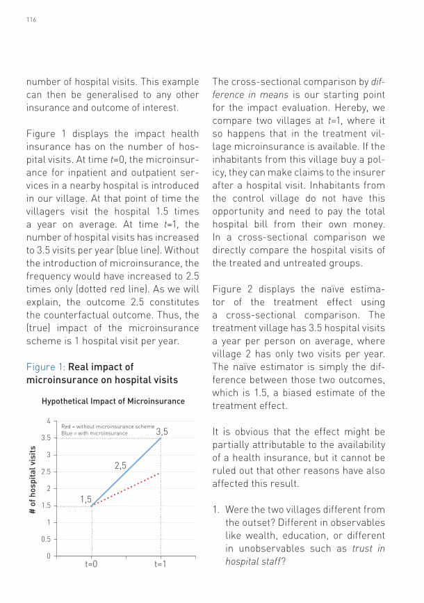
Figure 1 displays the impact health insurance has on the number of hos-pital visits. At time t=0, the microinsur-ance for inpatient and outpatient ser-vices in a nearby hospital is introduced in our village. At that point of time the villagers visit the hospital 1.5 times a year on average. At time t=1, the number of hospital visits has increased to 3.5 visits per year (blue line). Without the introduction of microinsurance, the frequency would have increased to 2.5 times only (dotted red line). As we will explain, the outcome 2.5 constitutes the counterfactual outcome. Thus, the (true) impact of the microinsurance scheme is 1 hospital visit per year.

Figure 1: Real impact of microinsurance on hospital visits

t=0 t=10

0.5

1

1.5

2

2.5

3

3.5

4

1,5

2,5

Red = without microinsurance schemeBlue = with microinsurance 3,5

# o

f hos

pita

l vis

its

Hypothetical Impact of Microinsurance

The cross-sectional comparison by dif-ference in means is our starting point for the impact evaluation. Hereby, we compare two villages at t=1, where it so happens that in the treatment vil-lage microinsurance is available. If the inhabitants from this village buy a pol-icy, they can make claims to the insurer after a hospital visit. Inhabitants from the control village do not have this opportunity and need to pay the total hospital bill from their own money. In a cross-sectional comparison we directly compare the hospital visits of the treated and untreated groups.

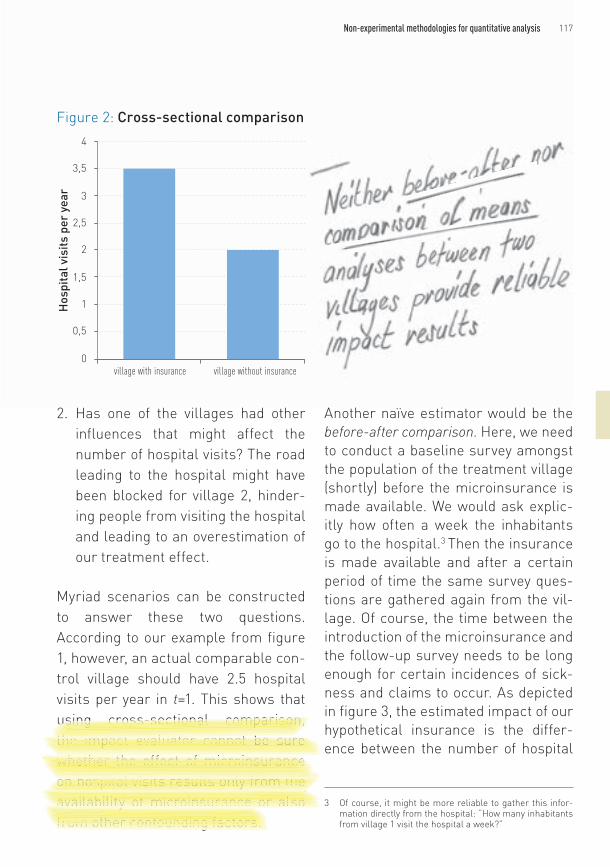
Figure 2 displays the naïve estima-tor of the treatment effect using a cross-sectional comparison. The treatment village has 3.5 hospital visits a year per person on average, where village 2 has only two visits per year. The naïve estimator is simply the dif-ference between those two outcomes, which is 1.5, a biased estimate of the treatment effect.

It is obvious that the effect might be partially attributable to the availability of a health insurance, but it cannot be ruled out that other reasons have also affected this result.

1. Were the two villages different from the outset? Different in observables like wealth, education, or different in unobservables such as trust in hospital staff?


2. Has one of the villages had other influences that might affect the number of hospital visits? The road leading to the hospital might have been blocked for village 2, hinder-ing people from visiting the hospital and leading to an overestimation of our treatment effect.

Myriad scenarios can be constructed to answer these two questions. According to our example from figure 1, however, an actual comparable con-trol village should have 2.5 hospital visits per year in t=1. This shows that using cross-sectional comparison, the impact evaluator cannot be sure whether the effect of microinsurance on hospital visits results only from the availability of microinsurance or also from other confounding factors.

Another naïve estimator would be the before-after comparison. Here, we need to conduct a baseline survey amongst the population of the treatment village (shortly) before the microinsurance is made available. We would ask explic-itly how often a week the inhabitants go to the hospital.3 Then the insurance is made available and after a certain period of time the same survey ques-tions are gathered again from the vil-lage. Of course, the time between the introduction of the microinsurance and the follow-up survey needs to be long enough for certain incidences of sick-ness and claims to occur. As depicted in figure 3, the estimated impact of our hypothetical insurance is the differ-ence between the number of hospital

3 Of course, it might be more reliable to gather this infor-mation directly from the hospital: “How many inhabitants from village 1 visit the hospital a week?”

Figure 2: Cross-sectional comparison

village with insurance village without insurance0

0,5

1

1,5

2

2,5

3

3,5

4

Hos

pita

l vis

its p

er y

ear

118

visits before and after introduction, which is two hospital visits per year. The interpretation would be that intro-ducing microinsurance that covers the cost of inpatient and outpatient care increases the number of hospital visits by two visits per year.

However, this estimator relies on the important assumption that, in between our two surveys, no other factors have occurred that might cause a change in hospital visits. This means that, for the before-and-after estimator to pro-duce reliable results, our researcher must be sure no other confounding effects have occurred between the two surveys. In fact, figure 1 shows that without microinsurance there still would have been an upwards trend in hospital visits and that, therefore, our before-after comparison deliv-ers unreliable results. Reasons for an upwards trend in hospital visits inde-pendent of the treatment could be increases in prosperity, decreases in transportation costs, and many other scenarios.

In sections 6.3 through 6.6 of this chap-ter, the following four non-experimen-tal approaches will be explained:

1. Instrumental variables 2. Regression discontinuity design

(RDD)3. Propensity score matching (PSM) 4. Difference-in-differences (DID)

Amongst them, the first two approaches, if applicable, usually give the most convincing results. We will also stress the importance of inter-nal and external validity in each case. Internal validity is the extent to which the results are credible for the popu-lation under consideration. External validity is the extent to which this sub-population is representative for the whole population (of interest). Some

Figure 3: Before-and-after comparison

Before After0

1

2

3

4

5

6

Hos

pita

l vis

its p

er y

ear

in tr

eatm

ent v

illag

e


methods give results with high internal validity, but low external validity, and vice versa. We conclude with a discus-sion of where non-experimental meth-ods should be applied.

6.3. Instrumental variable

Selection bias occurs when an omitted variable has an effect on the outcome variable of interest and the treatment. It is also called selection on unob-servables, whereby treatment selec-tion is affected by a variable that the researcher cannot observe in the data. For example, individuals with insurance could have had a higher (unobserved) awareness for health issues from the outset. Consequently, they would show different health behaviour, than those without insurance. Figure 4 illustrates this simple case with arrows indicating directions of influence and dashed lines indicating unobserved variables (health

awareness). The instrument affects insurance take-up without being itself affected by different levels of aware-ness about insurance. In the absence of a good instrument, one could not tell apart the insurance’s effect and the awareness’ effect on hospital visits. Instrumental variable methods solve this problem of omitted control variables. An instrumental variable is a variable which has an effect on whether an individual takes up or does not take up treatment and at the same time is per-mitted to affect the outcome variable of interest via the treatment variable only. This is called the exclusion restriction. In other words, individuals with different values of the instrument differ in their treatment status. But otherwise, these individuals are comparable. Often, the exclusion restriction will be only valid conditionally, that means when con-trolling for individual characteristics.

Figure 4: Setup with instrumental variable

Hospital visits

Instrument Insurance

Awareness

120

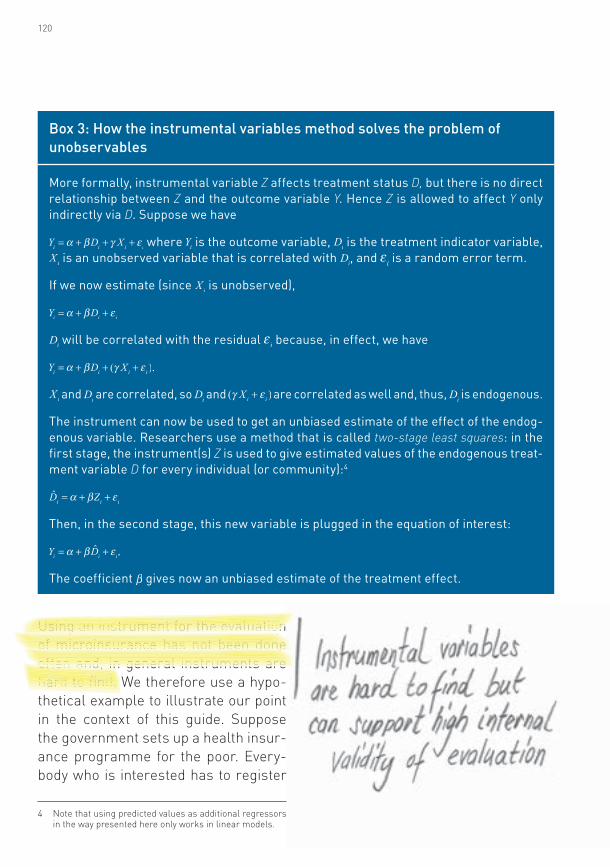
Box 3: How the instrumental variables method solves the problem of unobservables

More formally, instrumental variable Z affects treatment status D, but there is no direct relationship between Z and the outcome variable Y. Hence Z is allowed to affect Y only indirectly via D. Suppose we have

where is the outcome variable, is the treatment indicator variable, is an unobserved variable that is correlated with , and is a random error term.

If we now estimate (since is unobserved),

will be correlated with the residual because, in effect, we have

.

and are correlated, so and are correlated as well and, thus, is endogenous.

The instrument can now be used to get an unbiased estimate of the effect of the endog-enous variable. Researchers use a method that is called two-stage least squares: in the first stage, the instrument(s) Z is used to give estimated values of the endogenous treat-ment variable D for every individual (or community):4

Then, in the second stage, this new variable is plugged in the equation of interest:

.

The coefficient gives now an unbiased estimate of the treatment effect.

Using an instrument for the evaluation of microinsurance has not been done often and, in general instruments are hard to find. We therefore use a hypo-thetical example to illustrate our point in the context of this guide. Suppose the government sets up a health insur-ance programme for the poor. Every-body who is interested has to register

4 Note that using predicted values as additional regressors in the way presented here only works in linear models.


and purchase the product at the local insurance administration centre of the neighbourhood or municipality. Now imagine two households that are very close, but on different sides of the bor-der between two neighbourhoods. The distance to the administrative centre might differ considerably, but other-wise the two neighbours should be very similar. For such pairs, distance to the administrative centre could be used as a predictor of insurance take-up that is otherwise unrelated to individ-ual characteristics—in other words, a good instrument. Here, the instru-ment is correlated with insurance take-up but not with awareness. Thus, instead of comparing the treated to the untreated, we compare those with high values and low values of the instru-ment. This example is analogous to the famous distance-to-school instrument used by Card (1995) for schooling. Typi-cally, an instrument requires including additional X variables, e.g., quality of the neighbourhood, degree of urbani-sation, family background, etc.

We may also generate instrumen-tal variables ourselves by randomly assigning incentives or encourage-ments to individuals (random encour-agement design). This approach looks very much like a proper randomised experiment, except that we have imper-fect control over the beneficiaries. An encouragement or incentive is given to the individuals in the treatment group,

whilst the individuals in the control group do not receive such an encour-agement or incentive (or receive a dif-ferent one). It is up to the individuals whether they sign up for the actual treatment. For example, imagine that the price of insurance is varied ran-domly across communities, creating a random incentive to buy insurance for the population facing a lower price. The instrumental variable that is gen-erated here helps resolve the problem of selection bias and allows consistent estimation of the effect that insurance take-up has on health and other out-come measures. Similarly, we may vary the effort related to take-up by, for example, varying service hours, density of offices in a community, etc., from the insurer’s side. If areas or individuals cannot be exclusively chosen for a pro-gramme at random, we may at least give them varying incentives to do so.

If there is an instrument that fulfills the exclusion restriction as explained above, internal validity is high. How-ever, external validity depends on another quality of the instrument. If the instrument predicts treatment status accurately, external validity is also likely to be high. Otherwise the instrumental variable results cannot be generalised to the whole popula-tion. The reason is that only those who are induced to take up treatment by the instrument can be used for the estima-tion of the treatment effect.

122

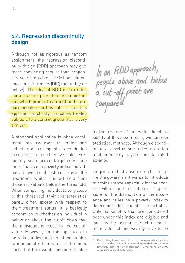
6.4. Regression discontinuity design

Although not as rigorous as random assignment, the regression disconti-nuity design (RDD) approach may give more convincing results than propen-sity score matching (PSM) and differ-ence-in-differences (DID) methods (see below). The idea of RDD is to exploit some cut-off point that is important for selection into treatment and com-pare people near this cutoff. Thus, this approach implicitly compares treated subjects to a control group that is very similar.

A standard application is when enrol-ment into treatment is limited and selection of participants is conducted according to an objective rule. Fre-quently, such form of targeting is done on the basis of a poverty index: individ-uals above the threshold receive the treatment, whilst it is withheld from those individuals below the threshold. When comparing individuals very close to this threshold, their characteristics barely differ, except with respect to their treatment status. It is basically random as to whether an individual is below or above the cutoff given that the individual is close to the cut-off value. However, for this approach to be valid, individuals must be unable to manipulate their value of the index such that they would become eligible

for the treatment. To test for the plau-sibility of this assumption, we can use statistical methods. Although disconti-nuities in evaluation studies are often unplanned, they may also be integrated ex-ante.

To give an illustrative example, imag-ine the government wants to introduce microinsurance especially for the poor. The village administration is respon-sible for the distribution of the insur-ance and relies on a poverty index to determine the eligible households. Only households that are considered poor under this index are eligible and can buy the insurance. Such disconti-nuities do not necessarily have to be

5 Even if they have some influence, the approach is feasible as long as they are unable to manipulate their assignment precisely. The solution in this case is the so-called fuzzy regression discontinuity design.

5


planned as part of the intervention (even though it is certainly beneficial to have it planned beforehand). Instead, the evaluator could detect and exploit any rule used in practice to determine participation in the programme.

Figure 5 shows the number of hos-pital visits by ranking in the poverty index sometime after the programme started in our hypothetical village.

We see that the number of hospital vis-its increases and that there is a jump exactly at the poverty line. This jump is a result of the microinsurance pro-gramme and the restriction that only poor people have access to this pro-gramme. Any household that is above the poverty line has no access to the insurance product. RDD assumes that households just above the poverty line are, in fact, similar to those slightly below the index in all relevant aspects.

Therefore, we can use the households that are eligible for the insurance and very close to the threshold as our treat-ment group, whilst those slightly above the threshold serve as control group.

The benefit of RDD is that it does not need actual randomisation. However, the interpretation of the estimated impact is limited to the population that is close to the threshold. As a result, external validity of this approach is rather limited. Further, it usually requires a large sample for estimation.

6.5. Propensity score matching (PSM)

The basic idea of propensity score matching is to match at least one non-participant to every participant with identical or highly similar values of observed characteristics X. The dif-ference in outcome, Y, between these

Figure 5: Regression discontinuity design

poor Poverty line rich

Hos

pita

l vis

its p

er y

ear

Poverty index

4

3.5

3

2.5

2

1.5

1

0.5

0

Dark blue = eligible for microinsurance schemeLight blue = not eligible for microinsurance scheme

124

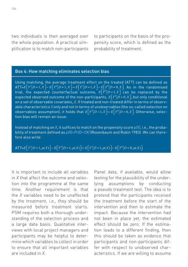
two individuals is then averaged over the whole population. A practical sim-plification is to match non-participants

to participants on the basis of the pro-pensity score, which is defined as the probability of treatment.

Box 4: How matching eliminates selection bias

Using matching, the average treatment effect on the treated (ATT) can be defined as ATT= . As in the randomised trial, the expected counterfactual outcome, can be replaced by the expected observed outcome of the non-participants, , but only conditional on a set of observable covariates, X. If treated and non-treated differ in terms of observ-able characteristics X only and not in terms of unobservables (the so-called selection on observables assumption), it holds that . Otherwise, selec-tion bias will remain an issue.

Instead of matching on X, it suffices to match on the propensity score p(X), i.e., the proba-bility of treatment defined as p(X)=Pr(D=1|X) (Rosenbaum and Rubin 1983). We can there-fore also write

ATT= .

It is important to include all variables in X that affect the outcome and selec-tion into the programme at the same time. Another requirement is that the X variables need to be unaffected by the treatment, i.e., they should be measured before treatment starts. PSM requires both a thorough under-standing of the selection process and a large data basis. Qualitative inter-views with local project managers and participants may be helpful to deter-mine which variables to collect in order to ensure that all important variables are included in X.

Panel data, if available, would allow testing for the plausibility of the under-lying assumptions by conducting a pseudo treatment test. The idea is to pretend that the participants received the treatment before the start of the intervention and then to estimate the impact. Because the intervention had not been in place yet, the estimated effect should be zero. If the estima-tion leads to a different finding, then this should be taken as evidence that participants and non-participants dif-fer with respect to unobserved char-acteristics. If we are willing to assume


that these differences are time-invari-ant, then we can use a DID matching approach. If, however, we suspect that these differences change over time, then we need more or better X vari-ables or a better understanding of the selection process.

Propensity score matching gives rather low internal validity due to its reliance on the selection on observ-ables assumption. In other words, the results might be biased if there are variables that are correlated with insurance take-up and the outcome of interest (such as hospital visits), but cannot be observed in the data. Exter-nal validity can be high, except in the case that we cannot find sufficiently comparable untreated individuals to be matched with every treated indi-vidual (the so-called common support requirement). These treated individ-uals would then need to be excluded from the analysis, which would reduce external validity.

6.6. Difference-in-differences (DID)

Relying on the assumption that selec-tion is on observables only can be

difficult to justify. Often we need a method that can also take care of confounding variables that are unob-served. However, as already men-tioned, good instruments are hard to find. Therefore, we would like have other tools to deal with unobservables. The DID estimator uses data with a time or cohort dimension to con-trol for unobserved but time-invariant variables. It relies on comparing par-ticipants and non-participants before and after the treatment. The minimum requirement is to have data on an out-come variable, Y, and treatment status, D, before and after the intervention. (It can be carried out with or without panel data and with or without con-trolling for characteristics, X.) In its simplest form, we take the difference in Y for the participants before and after the treatment and subtract the difference in Y for the non-participants before and after the treatment. As a result, time-invariant differences in characteristics between participants and non-participants are eliminated, allowing us to identify the treatment effect. Consequently, this approach accounts for unobserved heterogene-ity as long as it is time-invariant.

126

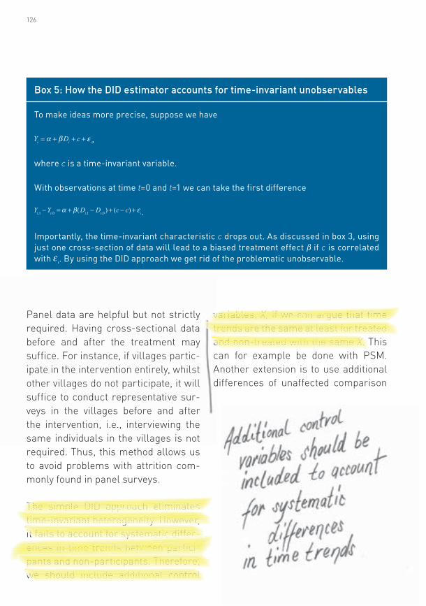
Panel data are helpful but not strictly required. Having cross-sectional data before and after the treatment may suffice. For instance, if villages partic-ipate in the intervention entirely, whilst other villages do not participate, it will suffice to conduct representative sur-veys in the villages before and after the intervention, i.e., interviewing the same individuals in the villages is not required. Thus, this method allows us to avoid problems with attrition com-monly found in panel surveys.

The simple DID approach eliminates time-invariant heterogeneity. However, it fails to account for systematic differ-ences in time trends between partici-pants and non-participants. Therefore, we should include additional control

variables, X, if we can argue that time trends are the same at least for treated and non-treated with the same X. This can for example be done with PSM. Another extension is to use additional differences of unaffected comparison

Box 5: How the DID estimator accounts for time-invariant unobservables

To make ideas more precise, suppose we have

,

where c is a time-invariant variable.

With observations at time t=0 and t=1 we can take the first difference

.

Importantly, the time-invariant characteristic c drops out. As discussed in box 3, using just one cross-section of data will lead to a biased treatment effect if c is correlated with . By using the DID approach we get rid of the problematic unobservable.


groups. For instance, imagine an insurance product applies only to indi-viduals below the age of 40. We can then compare the time trend of individ-uals above the age of 40 in the treat-ment villages with the time trend of those above 40 in the control villages. This difference in time trends can be used to eliminate differences in time trends of those under 40. A further possibility is to use data for more than one point in time before the treatment is introduced. This would also allow eliminating differences in time trends. Having more than one survey after the treatment implementation additionally allows the estimation of time-varying and long-run treatment effects.

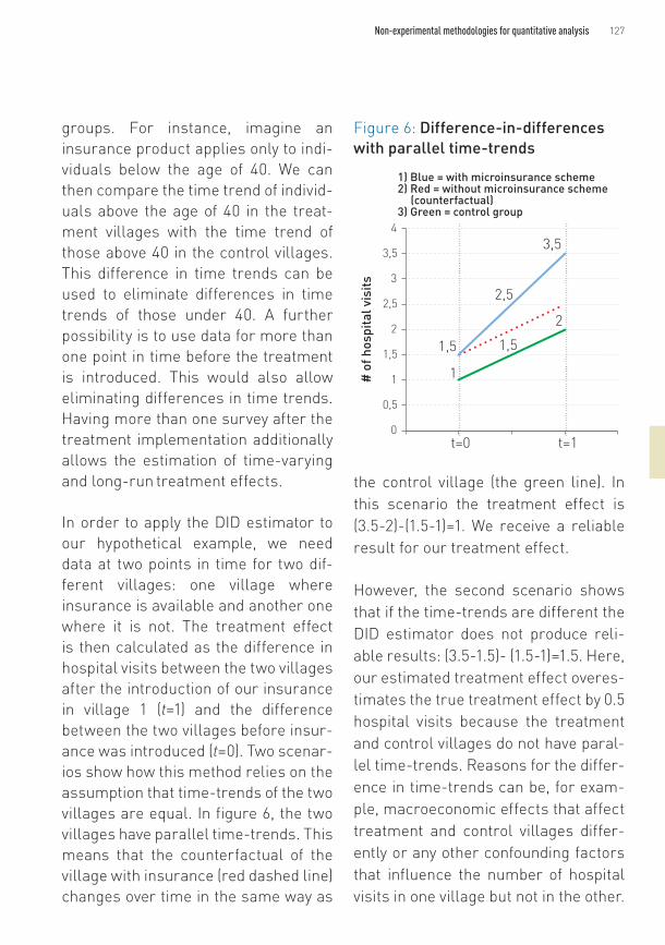
In order to apply the DID estimator to our hypothetical example, we need data at two points in time for two dif-ferent villages: one village where insurance is available and another one where it is not. The treatment effect is then calculated as the difference in hospital visits between the two villages after the introduction of our insurance in village 1 (t=1) and the difference between the two villages before insur-ance was introduced (t=0). Two scenar-ios show how this method relies on the assumption that time-trends of the two villages are equal. In figure 6, the two villages have parallel time-trends. This means that the counterfactual of the village with insurance (red dashed line) changes over time in the same way as

the control village (the green line). In this scenario the treatment effect is (3.5-2)-(1.5-1)=1. We receive a reliable result for our treatment effect.

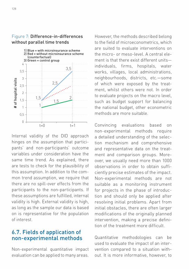
However, the second scenario shows that if the time-trends are different the DID estimator does not produce reli-able results: (3.5-1.5)- (1.5-1)=1.5. Here, our estimated treatment effect overes-timates the true treatment effect by 0.5 hospital visits because the treatment and control villages do not have paral-lel time-trends. Reasons for the differ-ence in time-trends can be, for exam-ple, macroeconomic effects that affect treatment and control villages differ-ently or any other confounding factors that influence the number of hospital visits in one village but not in the other.

Figure 6: Difference-in-differences with parallel time-trends

t=0 t=10

0,5

1

1,5

2

2,5

3

3,5

4

1,5

2,5

3,5

1

1,5

2

1) Blue = with microinsurance scheme2) Red = without microinsurance scheme (counterfactual)3) Green = control group

# o

f hos

pita

l vis

its

128

Internal validity of the DID approach hinges on the assumption that partici-pants’ and non-participants’ outcome variables under consideration have the same time trend. As explained, there are tests to check for the plausibility of this assumption. In addition to the com-mon trend assumption, we require that there are no spill-over effects from the participants to the non-participants. If these assumptions are fulfilled, internal validity is high. External validity is high, as long as the sample our data is based on is representative for the population of interest.

6.7. Fields of application of non-experimental methods

Non-experimental quantitative impact evaluation can be applied to many areas.

However, the methods described belong to the field of microeconometrics, which are suited to evaluate interventions on the micro- or meso-level. A central ele-ment is that there exist different units—individuals, firms, hospitals, water works, villages, local administrations, neighbourhoods, districts, etc.—some of which were exposed by the treat-ment, whilst others were not. In order to evaluate projects on the macro level, such as budget support for balancing the national budget, other econometric methods are more suitable.

Convincing evaluations based on non-experimental methods require a detailed understanding of the selec-tion mechanism and comprehensive and representative data on the treat-ment and comparison groups. More-over, we usually need more than 1000 observations in order to obtain suffi-ciently precise estimates of the impact. Non-experimental methods are not suitable as a monitoring instrument for projects in the phase of introduc-tion and should only be applied after resolving initial problems. Apart from initial obstacles, there are often larger modifications of the originally planned intervention, making a precise defini-tion of the treatment more difficult.

Quantitative methodologies can be used to evaluate the impact of an inter-vention compared to a situation with-out. It is more informative, however, to

Figure 7: Difference-in-differences without parallel time trends

t=0 t=10

0,5

1

1,5

2

2,5

3

3,5

4

1,5

2,5

3,5

11,5

2

1) Blue = with microinsurance scheme2) Red = without microinsurance scheme (counterfactual)3) Green = control group

# o

f hos

pita

l vis

its


evaluate the impact of an intervention relative to other interventions or, alter-natively, to evaluate different variants of an intervention, keeping context and data collection procedure constant. This, for example, would allow to look at the impact of different incentives or cost sharing arrangements for subsi-dised insurance.

Non-experimental methods gener-ally give less convincing results than experimental methods. Moreover, if the confidence intervals turn out to be very wide, we should not interpret these non-significant results as evi-dence for the absence of an impact. This interpretation is only valid if the confidence intervals are very narrow. The correct interpretation would be

that the sample size was too small to draw reliable conclusions.

References

Angrist, J. D. 2004. American education re-search changes track. Oxford Review of Econom-ic Policy 20(2):198-212.

Burtless, G. and L. L. Orr. 1986. Are classi-cal experiments needed for manpower policy? Journal of Human Resources 4:606-639.

Card, D. 1995. Earnings, schooling, and ability revisited. Research in Labor Economics 14:23-48.

Leeuw, F. and J. Vaessen. 2009. Impact evalua-tions and development: NONIE guidance on im-pact evaluation. Washington, D.C.: The Network of Networks on Impact Evaluation (NONIE). http://siteresources.worldbank.org/EXTOED/Resources/nonie_guidance.pdf

Rosenbaum, P. R. and D. B. Rubin. 1983. The central role of the propensity score in obser-vational studies for causal effects. Biometrika 70(1):41-55.

non-experimental methodologies for quantitative analysis

Documents