non-invasive measurement of the pressure distribution … · non-invasive measurement of the...

J. Fluid Mech. (2013), vol. 734, R1, doi:10.1017/jfm.2013.474

Non-invasive measurement of the pressuredistribution in a deformable micro-channelOzgur Ozsun, Victor Yakhot and Kamil L. Ekinci†

Department of Mechanical Engineering, Boston University, Boston, MA 02215, USA

(Received 11 June 2013; revised 5 August 2013; accepted 8 September 2013;first published online 7 October 2013)

Direct and non-invasive measurement of the pressure distribution in test sectionsof a micro-channel is a challenging, if not an impossible, task. Here, we presentan analytical method for extracting the pressure distribution in a deformable micro-channel under flow. Our method is based on a measurement of the channel deflectionprofile as a function of applied hydrostatic pressure; this initial measurement generates‘constitutive curves’ for the deformable channel. The deflection profile under flowis then matched to the constitutive curves, providing the hydrodynamic pressuredistribution. The method is validated by measurements on planar microfluidic channelsagainst analytic and numerical models. The accuracy here is independent of the natureof the wall deformations and is not degraded even in the limit of large deflections,ζmax/2h0 = O(1), with ζmax and 2h0 being the maximum deflection and the unperturbedheight of the channel, respectively. We discuss possible applications of the method incharacterizing micro-flows, including those in biological systems.

Key words: biological fluid dynamics, flow–vessel interactions, microfluidics

1. Introduction

Since the early experiment of Poiseuille (Sutera & Skalak 1993) more than twocenturies ago, the craft of measuring flow fields in tubes and pipes has been perfected.Even so, the resolution limits of these exquisite experimental probes, such as the Pitottube (McKeon 2007) or the hot-wire anemometer (Bruun 1995), are quickly beingapproached, given recent advances in micron- and nanometre-scale technologies. Onefrequently encounters micro- (Stone, Stroock & Ajdari 2004; Popel & Johnson 2005)and nano-flows (Schoch, Han & Renaud 2008), which come with smaller length scales(Lissandrello, Yakhot & Ekinci 2012) and shorter time scales (Ekinci, Karabacak &Yakhot 2008) than can be resolved by the commonly available probes. For instance, ina pressure-driven micro-flow, one must insert micron-scale pressure transducers in testsections in order to determine the local pressure drops (Kohl et al. 2005; Akbarian,

† Email address for correspondence: [email protected]

c© Cambridge University Press 2013 734 R1-1

mailto:[email protected]

O. Ozsun, V. Yakhot and K. L. Ekinci

Faivre & Stone 2006; Srivastava & Burns 2007; Hardy et al. 2009; Orth, Schonbrun& Crozier 2011; Song & Psaltis 2011). As the size of a probe becomes comparable toor even bigger than the flow scale itself, measurement of the distribution of flow fieldsbecomes problematic.

Although the tools of macroscopic fluid mechanics may not easily be scaled down,the materials and techniques of microfluidics offer unique measurement approaches.Most micro-channels in lab-on-chip systems, for instance, are made up of flexiblematerials (Whitesides & Stroock 2001; Gervais et al. 2006). This provides thepossibility of probing a flow by monitoring the response of the confining micro-channel to the flow. In other words, the local (position-dependent) deflection ζ of thedeformable walls of a micro-channel may enable the accurate determination of thepressure field (or the velocity field) under flow. The challenge in this approach, ofcourse, is characterizing the interactions between a deformable body and a flow (Hosoi& Mahadevan 2004; Shelley, Vanderberghe & Zhang 2005; Holmes et al. 2013). Thisis not a simple task, especially in the limit of large deflections. To accurately predicta flow bounded by a deformable wall, one needs to determine the hydrodynamicfields as well as the wall deformations consistently. This requires solving coupledfluid–structure equations (Pedley & Lou 1998; Heil & Jensen 2003), often in situationswhere constitutive relations or parameters describing fluid–structure interactions arenot available. Even if these relations and parameters are known, numerical approachesare often expensive.

To make the above discussion more concrete, let us consider a steady pressure-driven flow between an infinite rigid plate at y = 0 and a deformable wall aty = 2h0 + ζ(x), where ζ(x) is the local deflection of the deformable wall due tothe local pressure p(x) as shown in figure 1(a). The equations for incompressiblesteady flow (∂xu+ ∂yv = 0),

u∂xu+ v∂yu=−∂xp+ ν(∂x2 + ∂y

2)u, (1.1a)

u∂xv + v∂yv =−∂yp+ ν(∂x2 + ∂y

2)v, (1.1b)

are to be solved subject to boundary conditions u|B = v|B = 0. All the variables in(1.1) have their usual meanings (see figure 1a), with ν being the kinematic viscosity.In general, solutions to these equations, accounting for inlet and outlet effects, areimpossibly difficult. However, if the channel is long such that (2h0 + ζmax)/l� 1,where ζmax is the maximum deflection and l is the length of the channel, we can writethe local solution for the average velocity u(x) as

u(x)≈ 112η

[2h0 + ζ (p(x))]2∂xp. (1.2)

Here, η is the dynamic viscosity, and ζ(x) = ζ (p(x)) is a local constitutive relation,which determines the dependence of the wall deflection ζ(x) on p(x). No particularform for this dependence (e.g. elastic) is assumed a priori. In order to find theflow rate and the wall stresses, we need accurate information on p(x), ζ(x), and theconstitutive relation ζ(x) = ζ(p(x)). If the flow rate is given, the problem becomessomewhat simplified, but still remains rather complex to be handled numerically oranalytically.

In this paper, we describe a method to close (1.1) in a deformable channel usingindependent static measurements of ζ = ζ(p). Using this method, we extract the

734 R1-2

Non-invasive pressure measurements

(a) (b)

xz

y

05

1015

–0.5

00.5

z (m

m)

x (mm)0 5 10 15

–20

0

20

40

3.6 kPa

100 Pa

1.6 kPa

50 kPa

20 kPa

10 kPa

Chip

Bottom wall

ShimChannelz

y

(d)

(e) (f)

(c)

x

y

100

101

102

102 103 104 105 103 104 105

100

101

102

FIGURE 1. (a) A one-dimensional channel with a deformable top wall. (b) The two-dimensionaldeflection ζ2d(x, z) of S1 (t = 200 nm, 2h0 = 175 µm) under hydrostatic pressure of p = 2.3 kPaas measured optically. The inset shows a cross-sectional view of the channel. Clamps hold thechip (with the thin membrane at the centre) and the bottom wall together. The two walls areseparated by a precision shim; an O-ring (black ovals) seals the channel. (c) Cross-sectionalline scans from the image in (b) showing the parabolic z-profile of the deformable wall underpressure. (d) The one-dimensional (average) wall deflection ζ(x) at several different pressuresfor the same sample. The indicated values are gauge pressure values. These are the localconstitutive curves. (e) The peak deflection ζp of the PDMS deformable walls as a function ofpressure p. (f ) ζp of the SiN deformable walls as a function of p; the dashed lines are the p1/3

asymptotes. Note that the ζp and the p axes do not cover the same ranges in (e) and (f ). Errorbars are smaller than the symbols.

pressure distribution in a planar channel flow and validate our measurements againstthe analytic approximation in (1.2) for a long channel. Our method does not dependupon the particulars of the local constitutive relation ζ(x)= ζ(p(x)). In other words, itremains independent of the nature of the wall response, providing accurate results forbuckled walls and elastically stretching walls alike.

734 R1-3


Sample Material Wall Unperturbed Re Max. defl. Max. flow ratethickness height ζmax Qmax

t (µm) 2h0 (µm) (µm) (ml min−1)

S1 SiN 0.2 175 70–1200 33 70S2 SiN 1 180 100–1200 20 70S3 SiN 1 97 250–1300 37 70S4 PDMS 200 244 200–800 86 50S5 PDMS 605 155 200–900 25 50

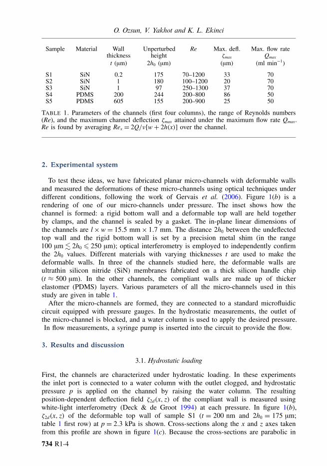
TABLE 1. Parameters of the channels (first four columns), the range of Reynolds numbers(Re), and the maximum channel deflection ζmax attained under the maximum flow rate Qmax.Re is found by averaging Rex = 2Q/ν[w+ 2h(x)] over the channel.

2. Experimental system

To test these ideas, we have fabricated planar micro-channels with deformable wallsand measured the deformations of these micro-channels using optical techniques underdifferent conditions, following the work of Gervais et al. (2006). Figure 1(b) is arendering of one of our micro-channels under pressure. The inset shows how thechannel is formed: a rigid bottom wall and a deformable top wall are held togetherby clamps, and the channel is sealed by a gasket. The in-plane linear dimensions ofthe channels are l×w= 15.5 mm× 1.7 mm. The distance 2h0 between the undeflectedtop wall and the rigid bottom wall is set by a precision metal shim (in the range100 µm. 2h0 6 250 µm); optical interferometry is employed to independently confirmthe 2h0 values. Different materials with varying thicknesses t are used to make thedeformable walls. In three of the channels studied here, the deformable walls areultrathin silicon nitride (SiN) membranes fabricated on a thick silicon handle chip(t ≈ 500 µm). In the other channels, the compliant walls are made up of thickerelastomer (PDMS) layers. Various parameters of all the micro-channels used in thisstudy are given in table 1.

After the micro-channels are formed, they are connected to a standard microfluidiccircuit equipped with pressure gauges. In the hydrostatic measurements, the outlet ofthe micro-channel is blocked, and a water column is used to apply the desired pressure.In flow measurements, a syringe pump is inserted into the circuit to provide the flow.

3. Results and discussion

3.1. Hydrostatic loading

First, the channels are characterized under hydrostatic loading. In these experimentsthe inlet port is connected to a water column with the outlet clogged, and hydrostaticpressure p is applied on the channel by raising the water column. The resultingposition-dependent deflection field ζ2d(x, z) of the compliant wall is measured usingwhite-light interferometry (Deck & de Groot 1994) at each pressure. In figure 1(b),ζ2d(x, z) of the deformable top wall of sample S1 (t = 200 nm and 2h0 = 175 µm;table 1 first row) at p= 2.3 kPa is shown. Cross-sections along the x and z axes takenfrom this profile are shown in figure 1(c). Because the cross-sections are parabolic in

734 R1-4


the z-direction, we define an average or one-dimensional wall deflection ζ(x) as

ζ(x)= 1w

∫ +w/2

−w/2ζ2d(x, z) dz≈ 2

3ζ2d(x, z= 0). (3.1)

Here, ζ2d(x, z= 0) is the maximum value of the parabolic cross-section, and the factor2/3 comes from the integration. Similarly defined ζ(x) will allow us to perform a one-dimensional analysis in the hydrodynamic case. In figure 1(d), we plot ζ(x) for thesame channel at several different hydrostatic pressures, 100 Pa 6 p 6 50 kPa. Theseare the position-dependent (local) constitutive curves. Because of the clamping stresses,the deformable wall is initially in a buckled state. At low p, the wall deformationremains in the negative-y direction. As p is increased, the wall response becomeselastic, and the wall stretches like a membrane. Also, a small asymmetry is noticeablein ζ(x), caused by the deformation of the silicon chip during clamping. Figures 1(e)and 1(f ) show the peak deflection ζp, which typically occurs at (x, z) ≈ (l/2, 0), as afunction of p for the elastomer (PDMS) and SiN walls, respectively. Each deformablewall in figure 1(e, f ) has a constitutive ζp versus p curve, determining the behaviourof the entire wall. The thin nitride walls shown in figure 1(f ) obey the well-knownelastic shell model at high p, ζp ∼ p1/3 (Small & Nix 1992). The elastomer walls infigure 1(e) follow a different power law from the SiN ones, presumably because theyare much thicker and bending dominates their deformation. There is no noticeableuniversality in the ζp versus p data, i.e. the nature of the wall response and thus theconstitutive relations are material and geometry (thickness) dependent. Our flow resultsbelow, however, remain independent of the wall response.

3.2. Flow measurementsNext, we perform flow measurements in each micro-channel. The results from allfive channels are shown in figure 2(a). In the experiments, we establish a constantvolumetric flow rate Q through each channel using a syringe pump and measurethe pressure drop between the inlet and outlet using a macroscopic transducer. Weprefer to plot Q as the independent variable because the experiments are performedby varying Q and measuring the pressure drop. In all measurements, a small pressuredrop occurs in the rigid inlet and outlet regions of the channel. This is because ofthe finite size of the connections to the macroscopic pressure transducers. Knowingthe geometry of the rigid regions, we determine the pressure drop in these regionsfrom flow simulations (see the Appendix for details). Subsequently, we subtract this‘parasitic pressure drop’ from the measured pressure drop. In summary, 1pt in theplots in figure 2(a) corresponds to the corrected pressure drop in the compliant sectionof the channel as measured by a macroscopic transducer (hence, the subscript ‘t’).Figure 2(b) shows the channel deflection ζ(x) at several different flow rates forS1 (t = 200 nm and 2h0 = 175 µm). Returning to table 1, we now clarify that ζmax

corresponds to the maximum deflection of the channel at the highest applied flow rate.

3.3. Simple fitsBefore we present our method for analysing the flow, we attempt to fit theexperimental 1pt versus Q data to the theory described above in (1.1)–(1.2). Becauseour channels have a finite width w, the result in (1.2) must be modified slightly. Thesimplest approach is to use a linear approximation for the local pressure drop basedon the hydraulic resistance per unit length, r(x), of the channel. In a long channelat low Reynolds number, ∂xp ≈ Qr(x). The total pressure drop between the inletand outlet can then be found as ≈Q

∫ l0 r(x) dx (Batchelor 1967). In our analysis, we

734 R1-5


0 20 40 60 80

0

20

40

60

1

10

100

10 1003

(a)

(b)

0 5 10 15

–10

0

10

20

30

x (mm)

FIGURE 2. (a) The pressure drop 1pt in the compliant sections of the micro-channels as afunction of flow rate Q. Error bars are smaller than the symbol sizes. The dashed lines show fitsbased on the hydraulic resistance of the micro-channel. The inset shows a double logarithmicplot of the same data. (b) The deflection profile ζ(x) of S1 (t = 200 nm, 2h0 = 175 µm) atdifferent Q. The profile is no longer uniform (cf. figure 1d) because of the position-dependentpressure p(x) in the channel.

approximate our channel as a channel of rectangular cross-section of w× 2h(x), where2h(x)= 2h0 + ζ(x). Then (Bruss 2008),

r(x)≈

1

1− 0.63(

2h(x)

w

) 12η

w[2h(x)]3 . (3.2)

734 R1-6


0 5 10 15–20

0

20

40(a)

(b) (c)

x (mm)

0 5 10 15

0

1

2

–10

–5

0

5

x (mm) x (mm)0 5 10 15

0

5

10

15

20

25

0

10

20

30

FIGURE 3. Determining the pressure gradient inside a micro-channel from hydrostaticmeasurements (S1, t = 200 nm, 2h0 = 175 µm). (a) The channel deflection profiles under twoflow rates (upper thick line, Q= 70 ml min−1; lower thick line, Q= 5 ml min−1) are overlaid ontop of the deflection profiles taken under different hydrostatic pressures (cf. figures 1d and 2b).(b) The data points (�) correspond to the pressure distribution p(x) in the test section (shadedregion) for a flow rate of Q = 5 ml min−1. To obtain p(x), the pressure values at the intersectionpoints in (a) are plotted as a function of x. A nonlinearity is noticeable in p(x) at x ≈ 7.5 mm,where the slope of the linear fit changes. (c) Similarly determined p(x) for Q = 70 ml min−1.The black line is a simple linear fit. The red lines in (b) and (c) are the deflection profiles of thechannel at the given flow rates. The error bars in the data (�) are estimated to be smaller thanthe symbol size. Also plotted (+) are results from simple flow simulations.

With the 2h(x) data available from optical measurements, we calculate r(x) andintegrate it along the length of the channel for all flow rates to find the pressuredrop. The calculated 1pt are shown in figure 2(a) as dashed lines. It is difficult todetermine the source of the disagreement between the data and the fits in some cases.The flow in the inlet and outlet regions may still be contributing to the error, even aftersubtraction. Another source of error may be the boundary between the compliant andrigid regions of the channel.

3.4. Measurement of the pressure distributionWe now turn to the main point of this paper. Our method is illustrated in figure 3.The curves in the background in figure 3(a) are the now-familiar ζ(x) curves of S1(t = 200 nm and 2h0 = 175 µm) under different hydrostatic pressures (cf. figure 1d).These serve as the constitutive curves. On top of these hydrostatic profiles, we overlaytwo different hydrodynamic profiles (thicker lines) at flow rates of Q = 5 ml min−1

and Q = 70 ml min−1. The assumption here is that, under equilibrium, ζ(x) only

734 R1-7


depends upon p(x), providing us with the constitutive relation ζ(x) = ζ(p(x)). Wedetermine the positions where the dynamic profiles intersect with the static profilesand read out the pressure values for each intersection position. In figure 3(b,c), we plotthese read-out pressure values using symbols (�) as a function of position for the twodifferent flow rates; solid (red) lines are the deflection profiles. Also plotted (+) areresults from simple flow simulations (see below for further discussion). In figure 3(b),a noticeable deviation from a linear pressure distribution is present, as captured bythe two black line segments with different slopes. The p(x) in figure 3(c) can beapproximated well by a linear fit (black line) to within our resolution. In the regionnear the boundaries (x= 0 mm and x= 15.7 mm), where significant pressure gradientsmust be present, it is not possible to obtain pressure readings. Thus, the test section isthe shaded regions in figure 3(b,c) away from the boundaries. We confirm that similarbehaviour is observed in all measurements on different channels.

Finally, we show that what is found above is indeed the pressure distribution inthe channel. First, we turn to the simple flow simulation results (shown by +) infigure 3(b,c). Here, we take a two-dimensional channel with two rigid walls, with thetop one having the experimentally measured profile ζ(x) and the bottom one being flat.We prescribe the velocity u at the inlet based on the experimental Q value. We thencalculate the pressure distribution in the channel with the outlet pressure set to zero(see the Appendix for more details). In figure 3(b), a small nonlinearity qualitativelysimilar to that observed in the experiment is noticeable. Between the experiment andthe simulation, there is a small but constant pressure difference (∼300 Pa), whichprobably mainly comes from the non-zero outlet pressure in the experiment. Infigure 3(c), we notice a constant pressure difference (∼500 Pa) between experimentand simulation as well; in addition, there is a larger pressure difference towards theinlet. The excess pressure observed in the experiment is probably the pressure thatis needed to keep the deformable wall stretched, as the deformability of the wall iscompletely ignored in the simulation. The wall is stretched more towards the inlet,hence the larger pressure difference. (We estimate that this tension is not present in thebuckled wall of figure 3b.) Overall, the agreement is quite satisfactory.

We can further validate the extracted pressure drop 1pe across the (entire)deformable test section against the analytical approximation in (1.2). Our methodprovides 1pe directly for each flow rate. We illustrate this in figure 3(b): we take thehigh and low pressure values at the beginning and end of the test section, and calculatethe difference to find 1pe, i.e. 1pe = p(x ≈ 1.6 mm) − p(x ≈ 13 mm). Against this1pe value, we plot QR, where R is the hydraulic resistance of the channel for only theregion where the pressure drop is determined, i.e. the hydraulic resistance of the testsection. For the data in figure 3(b), for instance, R= ∫ x≈13 mm

x≈1.6 mm r(x) dx, where r(x) is theresistance per unit length given in (3.2). QR versus 1pe data for each channel and flowrate are shown in figure 4. The error bars are due to the propagated uncertainties in themeasurements of 2h0 + ζ(x).4. Conclusions and outlook

The agreement in figures 3 and 4 provides validation for our method and gives usconfidence that we can measure p(x) in deformable channels accurately. For the proof-of-principle demonstration in this paper, we have applied our method to a flow whichcan be approximated by the Poiseuille equation, i.e. (1.2) and (3.2). However, themethod should remain accurate independent of the nature of the flow (e.g. turbulentflows, flows with nonlinear p(x) or separated flows) because p(x) simply comes from

734 R1-8


1 10 100

1

10

100

FIGURE 4. Calculated pressure drop QR in the test section as a function of the extractedpressure drop 1pe. The symbols match with those used in figure 2(a). Representative error barsare due to the uncertainties in 2h0 + ζ(x). The solid line is QR=1pe.

the wall response, as evidenced by the nonlinear p(x) resolvable in figure 3(b). It mustalso be re-emphasized that the nature of the wall response is not of consequence aslong as the deflection is a continuous function – any function – of pressure, ζ = ζ(p).All these suggest that the method can be applied universally as an accurate probe offlows with micron, and even possibly sub-micron, length scales.

Our results may be related to prior studies on collapsible tubes (Carpenter & Pedley2003; Heil & Jensen 2003). For our system in two dimensions, in the case of smalldisplacements, ζ/2h0� 1, one can write a ‘tube law’

p= p(ζ, ζ ′′)≈ aζ + bζ ′′, (4.1)

which relates the local gauge pressure p (the so-called transmural pressure) to thechannel deflection ζ and its axial derivative ζ ′′ = d2ζ/dx2. In analogous expressionsin the collapsible tube literature, the coefficient a is typically found by consideringthe changes in the cross-sectional area; however, finding b, which determines theeffect of the axial tension on p, is typically not simple and is possible only forcertain tube geometries, e.g. for elliptic tubes (Whittaker et al. 2010). Several pointsare noteworthy about our experiments. First, the axial tension term appears to beunimportant here, i.e. p = p(ζ ). Second, the method remains accurate even whenζ ∼ 2h0. Finally, a method similar to the one described here may be useful fordetermining b experimentally for different geometries and large deformations.

We mention in passing that the friction drag in a channel with rigid walls separatedby a gap of 2h0 is larger than that in a deformable channel with the same unperturbedgap. To see this, consider a one-dimensional flow with a flux q per unit width. Thestress at the rigid wall is τ = −η∂yu|wall = h0∂xp. But q = (2h0

3/3η)∂xp. Therefore,τ = 3η2q/2h0

2. Given that q/h02 > q/(h0 + ζ/2)2, drag is reduced. We also note that

no evidence of transition to turbulence has been observed in our experiments even atthe largest Re≈ 1200.

734 R1-9


This non-invasive method can possibly find applications in characterizingphysiological flows. In blood flow in arteries (Ku 1997) and smaller vessels (Popel& Johnson 2005), flow–structure interactions are critical in determining functionality(Heil 1997; Heil & Jensen 2003; Grotberg & Jensen 2004). Using our method, forexample, one could extract the local pressure distribution in an arterial aneurysm,where the arterial wall degrades and eventually ruptures due to the pressure and shearforces during blood flow (Lasheras 2007).

The spatial resolution in a p(x) measurement depends upon the resolution in ζ , thenoise in the hydrostatic pressure measurement, and the magnitude of the response ofthe wall. With our current imaging system, we can detect deflections with .20 nmprecision, and the r.m.s. noise in the hydrostatic pressure transducer is ∼10 Pa. Bycollecting the constitutive curves in figure 3(a) at smaller pressure intervals, weestimate that we can measure p(x) with ∼10 µm resolution in this particular channel.This method can easily be scaled down to provide sub-micron resolution in a nano-fluidic channel by employing a higher numerical aperture objective. It may also bepossible to extend the method to study time-dependent fluid–structure interactions(Huang 2001; Bertram & Tscherry 2006) by collecting surface deformation mapsfaster (Sampathkumar, Ekinci & Murray 2011). By optimizing the averaging time,one should be able to collect high-speed high-resolution pressure measurements inminiaturized channels. Such advances could open up many other interesting fluiddynamics problems, especially in biological systems.

Acknowledgements

We acknowledge generous support from the US NSF through Grant No. CMMI-0970071. We thank Mr L. Li for help with the flow simulations.

Appendix

Pressure drops in the rigid inlet and outlet regions of the channels are deduced fromflow simulations in Comsol Multiphysics R© using the single-phase three-dimensionalsteady laminar flow environment. A constant volumetric flow rate is applied at theinlet port, and the pressure at the outlet port is kept at zero. All the channel wallsare assigned the no-slip boundary condition. We use quadrilateral mesh elements andincrease the mesh density until the results converge. The two-dimensional simulationsshown in figure 3(b,c) between the deformed top wall and the flat bottom wall arecarried out using the same single-phase steady laminar flow environment. The uppercompliant wall is replaced with a rigid wall, but the deformed wall shape is preservedby importing the experimental profile into the simulation. At the inlet port, instead ofvolumetric flow rate, the calculated flow velocity corresponding to the experimentalvolumetric flow rate is used.

References

AKBARIAN, M., FAIVRE, M. & STONE, H. A. 2006 High-speed microfluidic differential manometerfor cellular-scale hydrodynamics. Proc. Natl Acad. Sci. USA 103, 538–542.

BATCHELOR, G. K. 1967 An Introduction to Fluid Dynamics. Cambridge University Press.BERTRAM, C. D. & TSCHERRY, J. 2006 The onset offlow-rate limitation and flow-induced

oscillations in collapsible tubes. J. Fluids Struct. 22, 1029–1045.BRUSS, H. 2008 Theoretical Microfluidics. Oxford University Press.

734 R1-10


BRUUN, H. H. 1995 Hot-wire Anemometry: Principles and Signal Analysis. Oxford UniversityPress.

CARPENTER, P. W. & PEDLEY, T. J. (Eds) 2003 IUTAM Symposium on Flow Past HighlyCompliant Boundaries and in Collapsible Tubes. Kluwer.

DECK, L. & DE GROOT, P. 1994 High-speed noncontact profiler based on scanning white lightinterferometry. Appl. Opt. 33, 7334–7338.

EKINCI, K. L., KARABACAK, D. M. & YAKHOT, V. 2008 Universality in oscillating flows. Phys.Rev. Lett. 101, 264501.

GERVAIS, T., EL-ALI, J., GUNTHER, A. & JENSEN, F. K. 2006 Flow-induced deformation ofshallow microfluidic channels. Lab on a Chip 6, 500–507.

GROTBERG, J. B. & JENSEN, O. E. 2004 Biofluid mechanics in flexible tubes. Annu. Rev. FluidMech. 36, 121–147.

HARDY, B. S., UECHI, K., ZHEN, J. & KAVEHPOUR, H. P. 2009 The deformation of flexiblePDMS microchannels under a pressure driven flow. Lab on a Chip 9, 935–938.

HEIL, M. 1997 Stokes flow in collapsible tubes: computation and experiment. J. Fluid Mech. 353,285–312.

HEIL, M. & JENSEN, O. 2003 Flows in deformable tubes and channels – theoretical models andbiological applications. In IUTAM Symposium on Flow Past Highly Compliant Boundaries andin Collapsible Tubes (ed. P. W. Carpenter & T. J. Pedley), chap. 2, pp. 15–50. Kluwer.

HOLMES, D. P., TAVAKOL, B., FROEHLICHER, G. & STONE, H. A. 2013 Control and manipulationof microfluidic flow via elastic deformations. Soft Matter 9, 7049–7053.

HOSOI, A. E. & MAHADEVAN, L. 2004 Peeling, heeling, and bursting in a lubricated elastic sheet.Phys. Rev. Lett. 93, 137802.

HUANG, L. 2001 Viscous flutter of a finite elastic membrane in Poiseuille flow. J. Fluids Struct. 15,1061–1088.

KOHL, M. C., ABDEL-KHALIK, S. I., JETER, S. M. & SADOWSKI, D. L. 2005 A microfluidicexperimental platform with internal pressure measurements. Sensors Actuators A Phys. 118,212–221.

KU, D. N. 1997 Blood flow in arteries. Annu. Rev. Fluid Mech. 29, 399–434.LASHERAS, J. C. 2007 The biomechanics of arterial aneurysms. Annu. Rev. Fluid Mech. 39,

293–319.LISSANDRELLO, C., YAKHOT, V. & EKINCI, K. L. 2012 Crossover from hydrodynamics to the

kinetic regime in confined nanoflows. Phys. Rev. Lett. 108, 084501.MCKEON, B. J. 2007 Velocity, vorticity, and Mach number. In Springer Handbook of Experimental

Fluid Mechanics (ed. A. Yarin, C. Tropea & J. F. Foss), chap. 5, pp. 215–471. Springer.ORTH, A., SCHONBRUN, E. & CROZIER, K. B. 2011 Multiplexed pressure sensing with elastomer

membranes. Lab on a Chip 11, 3810–3815.PEDLEY, T. & LOU, X. Y. 1998 Modelling flow and oscillations in collapsible tubes. Theor. Comput.

Fluid Dyn. 10, 277–294.POPEL, A. S. & JOHNSON, P. C. 2005 Microcirculation and hemorheology. Annu. Rev. Fluid Mech.

37, 43–69.SAMPATHKUMAR, A., EKINCI, K. L. & MURRAY, T. W. 2011 Multiplexed optical operation of

distributed nanoelectromechanical systems arrays. Nano Lett. 11, 1014–1019.SCHOCH, R. B., HAN, J. & RENAUD, P. 2008 Transport phenomena in nanofluidics. Rev. Mod.

Phys. 80, 839–883.SHELLEY, M., VANDERBERGHE, N. & ZHANG, J. 2005 Heavy flags undergo spontaneous

oscillations in flowing water. Phys. Rev. Lett. 94, 094302.SMALL, M. K. & NIX, W. D. 1992 Analysis of the accuracy of the bulge test in determining the

mechanical properties of thin films. J. Mater. Res. 7, 1553–1563.SONG, W. & PSALTIS, D. 2011 Optofluidic membrane interferometer: a imaging method for

measuring microfluidic pressure and flow rate simultaneously on a chip. Biomicrofluidics 5,044110.

SRIVASTAVA, N. & BURNS, M. A. 2007 Microfluidic pressure sensing using trapped aircompression. Lab on a Chip 7, 633–637.

734 R1-11


STONE, H. A., STROOCK, A. D. & AJDARI, A. 2004 Engineering flows in small devices:microfluidics toward a lab-on-a-chip. Annu. Rev. Fluid Mech. 36, 381–411.

SUTERA, S. P. & SKALAK, R. 1993 The history of Poiseuille’s law. Annu. Rev. Fluid Mech. 25,1–20.

WHITESIDES, G. M. & STROOCK, A. D. 2001 Flexible methods for microfluidics. Phys. Today 54,42–48.

WHITTAKER, R. J., HEIL, M., JENSEN, O. E. & WATERS, S. L. 2010 A rational derivation of atube law from shell theory. Q. J. Mech. Appl. Maths 63, 465–496.

734 R1-12

non-invasive measurement of the pressure distribution … · non-invasive measurement of the...

Documents