non - isothermal film blowing process stability analysis ... · cooled to solid film. air is...
TRANSCRIPT

Non - Isothermal Film Blowing Process Stability Analysis for Non - Newtonian Fluids by using Variational Principles
Bc. Roman Kolařík
Master thesis 2008


ABSTRAKT
Tato práce se zabývá problematikou vzniku nestabilního rukávu při výrobě fólií
vyfukováním, a to s cílem stanovit stabilitní diagramy hodnotící vliv procesních podmínek,
designu vytlačovací hlavy a tokových charakteristik polymerů za předpokladu
neizotermálních podmínek. Za tímto účelem byl použit model, který pohlíží na existenci
stabilního procesu vyfukování jako na stav, který odpovídá minimálním energetickým
nárokům. Teoretické závěry byly následně porovnány s odpovídajícími experimentálními
daty pro lineární a různě rozvětvené polyolefiny a bylo zjištěno, že predikce použitého
modelu jsou v dobré shodě s experimentální realitou pro různé procesní podmínky.
Nejdůležitějším závěrem celé práce je zjištění, že vztah mezi stabilitou procesu vyfukování
a větvením polymeru má nemonotónní charakter.
Klíčová slova: Vyfukování, vytlačování, polymer, modelování polymerních procesů,
stabilitní analýza.

ABSTRACT
In this work, film blowing stability analysis has been performed theoretically by
using minimum energy approach for non-Newtonian polymer melts considering
non-isothermal processing conditions with the aim to understand the complicated link
between processing conditions, machinery design and material properties. Specific
attention has been paid to the investigation of the complicated links between polymer melt
rheology (extensional strain hardening/thinning, shear thinning, flow activation energy,
Newtonian viscosity, melt strength), processing conditions (heat transfer coefficient, mass
flow rate, die exit temperature, cooling air temperature) and film blowing stability. It has
been found that the theoretical conclusions are in very god agreement with the
experimental reality supporting the validity of the used numerical approach and film
blowing model. The most important conclusion from this work is theoretically and
experimentally supported finding that dependence between long chain branching and
bubble stability is non-monotonic.
Keywords: Blown film, extrusion, polymer, modeling of polymer processing, stability
analysis.

ACKNOWLEDGEMENTS
Here, I would like to take the opportunity to say: “Thank you very much, all of you who
helped me with my Master thesis.”
I would like to express my gratitude to prof. Ing. Martin Zatloukal, Ph.D. for his advice,
support and patience all the time of the work on my thesis.
My acknowledgement also belongs to doc. Ing. Anežka Lengálová, Ph.D., who helped me
significantly during the creation of my theoretical part.
And last but not least, I am indebted to my beloved family for their interest in my work,
and all the friends, especially Jan Musil, for their support.
I agree that the results of my Master thesis can be used by my supervisor’s decision. I will
be mentioned as a co-author in case of any publication.
I declare I worked on this Master thesis by myself and I have mentioned all the used
literature.
Zlín, May 22, 2008 ….…………………………………….
Roman Kolařík

CONTENTS
INTRODUCTION ............................................................................................................... 9 I THEORETICAL BACKGROUND ........................................................................ 11 1 THE FILM BLOWING PROCESS ........................................................................ 12
1.1 DESCRIPTION OF THE FILM BLOWING LINE ............................................................ 12 1.2 THE PROCESS DESCRIPTION .................................................................................. 13 1.3 BUBBLE INSTABILITIES ......................................................................................... 18
1.3.1 Draw resonance ............................................................................................ 19 1.3.2 Helical instability ......................................................................................... 20 1.3.3 Instability of the freeze line height (FLH instability) .................................. 21 1.3.4 Heavy-bubble instability .............................................................................. 21 1.3.5 Bubble flutter ............................................................................................... 22 1.3.6 Bubble breathing .......................................................................................... 23 1.3.7 Bubble tear ................................................................................................... 23 1.3.8 The area of stable and unstable bubbles ....................................................... 25
2 STABILIZATION OF THE FILM BLOWING PROCESS ................................ 28 2.1 BUBBLE STABILIZATION BY COOLING SYSTEM (MELT AREA) ................................ 28
2.1.1 External cooling system – air ring ............................................................... 29 2.1.2 Internal bubble cooling system .................................................................... 31 2.1.3 Venturi and Coanda effects .......................................................................... 32
2.2 BUBBLE STABILIZATION BY MECHANICAL PARTS (SOLID AREA) ........................... 34 2.2.1 Iris ................................................................................................................ 34 2.2.2 Bubble guides ............................................................................................... 35 2.2.3 Bubble calibration cage ................................................................................ 36
3 MODELING OF THE FILM BLOWING PROCESS ......................................... 38 3.1 REVIEW OF THE CURRENT MODELS ....................................................................... 38 3.2 PEARSON AND PETRIE FORMULATION................................................................... 40 3.3 ZATLOUKAL AND VLCEK FORMULATION .............................................................. 44
3.3.1 Bubble without neck .................................................................................... 46 3.3.2 Bubble with neck .......................................................................................... 48 3.3.3 High stalk bubble ......................................................................................... 51 3.3.4 Stability diagram .......................................................................................... 53 3.3.5 Energy equation ........................................................................................... 55 3.3.6 Constitutive equations .................................................................................. 56 3.3.7 Velocity profile ............................................................................................ 57 3.3.8 Numerical scheme ........................................................................................ 59
4 AIMS OF THE WORK ........................................................................................... 61 II EXPERIMENTAL ................................................................................................... 62 5 MATERIAL .............................................................................................................. 63 6 FILM BLOWING EXPERIMENT ...................................................................... 64 RESULTS AND DISCUSSION ........................................................................................ 67
THEORETICAL FILM BLOWING STABILITY ANALYSIS ......................................................... 67 COMPARISON BETWEEN EXPERIMENTAL AND THEORETICAL FILM BLOWING STABILITY ANALYSIS ........................................................................................................ 72

CONCLUSION .................................................................................................................. 74 BIBLIOGRAPHY ............................................................................................................ 109 LIST OF SYMBOLS ....................................................................................................... 114 LIST OF FIGURES ......................................................................................................... 119 LIST OF TABLES ........................................................................................................... 123 LIST OF APPENDICES ................................................................................................. 125

9
INTRODUCTION
Although the tubular film blowing process belongs to the oldest polymer processing
technologies, the process is still the most widely and frequently used technology to
produce thin thermoplastic films, mostly polyethylene. The first commercial film blowing
line was constructed in the late 1930´s in the USA and since then the technology has been
developing continuously [1, 2].
Film blowing lines produce biaxially oriented films of small thickness, which are
used in commodity applications. Thus, the film can be used in food processing industry,
e.g. for carrier bags and food wrapping, in the waste industry such as garbage bags or
waste land fill liners. Other applications are medical films or scientific balloons [1-3].
The film blowing process has been researched experimentally and theoretically
during a long history. However, clear relationships between the machine design,
processing parameters, material and stresses have not been fully explained yet. Moreover,
the film blowing process is affected by the creation of the bubble instabilities at particular
processing conditions, which is one of the limiting factors for the process. To understand
these instabilities in more detail, modeling of the film blowing process is usually used.
For this purpose the Pearson and Petrie formulation [1], as a classical method, is
usually employed. However, the use of the formulation leads to variety of the numerical
instabilities [4] and the experimental reality is not described very well, mainly in the case
of the bubble with neck [5]. These difficulties can be overcome by the utilization of
recently proposed Zatloukal-Vlcek film blowing model [6-9] derived through variational
principles which is capable to predict bubble shape (and corresponding processing
conditions) which satisfies the minimum energy requirements. Recently, it has been
demonstrated for isothermal conditions and Newtonian fluids that the stable film blowing
process can be viewed as the state which, firstly, satisfies minimum requirements and
secondly, does not yields the bubble machine and circumference stresses higher than the
rupture stress [2].
In order to extend the knowledge about the film blowing instabilities, non-isothermal
Zatloukal-Vlcek model for non-Newtonian polymer melts will be utilized to understand the
effect of heat transfer coefficients, melt/air temperature, flow activation energy, MWD,
shear thinning, extensional strain hardening/thinning on the film blowing stability. Special

10
attention will be paid to understand the complicated link between long chain branching and
film blowing stability from both, theoretical and experimental point of view.

11
I. THEORETICAL BACKGROUND

12
1 THE FILM BLOWING PROCESS
The film blowing process is predominantly used for the production of thin
biaxially-oriented thermoplastic films, especially from polyolefines on the film blowing
line, which is described here in more detail.
1.1 Description of the film blowing line
The most often used film blowing line type consist of the nip rollers which are
situated on the top of the line, as depicted in Fig. 1 [1,2, 10].
Fig. 1. Film blowing line
The film blowing process description is provided in the next section in more detail.
HOPPER PELLETS
WIND-UP DEVICE
GUIDE ROLL NIP ROLLS
ANNULAR DIE
AIR (COOLING) RING
FREEZE LINE HEIGHT
FILM
TABLE FLAP
AIR
SCREW EXTRUDER
IBC SYSTEM
CALIBRATION CAGE

13
1.2 The process description
At the beginning of the film blowing process, when the film is first extruded, film
cylindrical-tube is necessary to close. Thus, from the annular die, the tube end is capped
and tied to a rope. Then, it is drawn upward towards the nip rollers. This action must be
provided very carefully to prevent the tube from tearing. When the tube achieves the nip
rollers, it is sealed by the pinching action of the rollers. Then, it is fluently moved towards
to the wind up device. During the action, pressurized air is blown into the tube to inflate it
into a bubble, as can be seen in Fig. 2 [11]. The amount of air and the nip roller speed are
adjustable parameters which are important from the bubble stability point of view [11].
Fig. 2. Procedure used to start the film blowing process
The tubular film blowing process belongs to continual methods of the film
production. In this regard, the chamber of the solid polymer pellets is set on the start of the
film blowing line. Thus, continuous material feed to a hopper of the extruder is established
14
by a material handling system, such as silo and pneumatic loader. The hopper holds the
solid material and is cooled for the following two reasons. First, the friction between the
pellets is bigger if they are colder, i.e. more rigid. This ensures higher extruder output.
Second, hopper cooling limits creation of the pellets dome, which can cause shut-down of
the film blowing process. Then, pellets go through the hopper to the thread of the screw.
There, with the help of the barrel, pellets are transported, homogenized, compressed and
melted. The energy necessary for heating the pellets is obtained by dissipation and from
the heating elements along the barrel. During the process the required constant temperature
of every zone is kept by cooling fans along the barrel.
At the end of the barrel, the polymer pellets are molten and the melt is extruded
through an annular die. Hence, the film is created to shape continuous cylinder by the
internal air pressure. The cylinder moves in the vertical direction upwards. In the area
between the annular die (die exit) and the freeze line the polymer is in a molten state. With
the help of a cooling ring (with/without internal bubble cooling system IBC) the bubble is
cooled to solid film. Air is uniformly blown along the bubble surface. A constant diameter
of the created film bubble is kept by a calibration bubble cage. This cooling bubble is
folded between two table flaps and then two nip rollers close it. In the next step control of
film dimensions is performed, i.e. thickness and width of the layflat film is measured. Film
thickness is determined by the nip roll speed and also by the internal air pressure. After the
dimensions control the final film can be one-side or two-side split (see Appendix PI for
more detailed process description). The product is thin film. In the other cases (when a
cutting mechanism is not used), the final film can be used as a bag. Finally, the film is
spooled on the cylinder of a wind-up device where it is cut on a required length by a radial
cutting mechanism [3, 11-17].
The most frequently used polymers for the film blowing process are polyolefins,
such as LDPE, LLDPE and HDPE. Sometimes, also other materials are used, for example
ethylene copolymers, polypropylene copolymers, nylon, elastomers, nitriles or
polycarbonate [11].
The film blowing process is characterized by the below stated important parameters
and equations which describe bubble geometry during the process [3, 11, 13, 15]. The
parameters influence the area between the die exit and nip rollers, as shown in Fig. 3 [13].

15
Fig. 3. Elements of blown film
The most important film blowing process parameters are described below in more detail.
Blow up ratio
Blow up ratio, BUR, shows the size of the melt stretching in the transverse direction.
Blow-up ratio is expressed as the ratio of the final bubble diameter at the freeze line height,
Df, to the bubble diameter at the die exit, Dd, so it has the following form:
d
f
DD
BUR = (1)
In the case when the line is running, the final bubble diameter is difficult to measure.
Hence, the blow-up ratio is rewritten as
Dd td
Df
layflat width
vd
vf
ρm
ρs
Af
Ad
tf
L
vf

16
dDwidthlayflatBUR
π 2 ⋅
= (2)
Die diameter is fixed and it is identified by the producer of the die. The most
frequent blow-up ratio is in the range of 2 to 10.
Take-up ratio
The take-up ratio, TUR, is calculated as the ratio of the film velocity above the freeze
line (nip velocity), vf, to melt velocity through die exit, vd. This is a parameter determining
melt stretching in the machine direction. It can be written in the following form:
d
f
vv
TUR = (3)
During the film blowing process, the melt velocity is difficult to measure. Then, it is
possible to use the equation of conservation of mass with the condition that the mass flow
rate is constant along the bubble. Thus, the take-up ratio is
fs
dm
AA
TURρρ
= (4)
where ρm is the polymer melt density, ρs means the solid polymer density, and Ad and Af
represent the die gap area and bubble cross-sectional area, respectively.
Draw-down ratio
Draw-down ratio, DDR, shows stretching in the machine direction. It is possible to
express the total degree of film stretching because the thickness reduction occurs in the
transverse and machine direction at the same time. DDR describes the thickness reduction
from the die gap thickness, td, to the final film thickness, tf.
BURtt
DDRf
d= (5)
Draw-down ratio is more preferred than take-up ratio because it is easier to measure.
The value of DDR, as well as TUR, is from 5 to 20.

17
Forming ratio
Forming ratio, FR, expresses the relation between the take-up ratio and the blow-up
ratio. Thus, it gives a balance of process stretching.
BURTURFR = (6)
In the case when the forming ratio is equal to one, the mechanical properties in the
machine and transverse directions are the same, i.e. the film is isotropic. FR is only used
for general information about the molecular orientation and balance because the
relationship between them is not precise.
The blow-up ratio together with the draw-down ratio describe two directions of the
bubble extension in the area where the bubble is in a molten state. Thus, above the freeze
line the biaxial orientation is insignificant. The film is oriented in the axial direction by the
nip rollers with adjustable velocity. Then, this is one of the possibilities to change the film
thickness. The second extension direction is circumferential, and is generated by the air
pressure inside the bubble. So, the axial and circumferential extensions produce the final
shape and thickness of the bubble. The bubble geometry is then affected by the change of
the process conditions, as shown in Tab. 1 [3]. The table describes what will happen with
the film thickness, bubble diameter and the freeze line height if one of the process
variables increases. Here, the bigger and bold symbols represents a significant change in
the bubble geometry during the increase of the given process parameter.
Tab. 1. The effect of major process variables on bubble geometry.
Variable to increase Film thickness Bubble diameter Freeze line height
Nip speed ↓ ↑ ↑
Screw speed ↑ ↑ ↑
Cooling speed ↑ ↓ ↓ Bubble volume ↓ ↑ ↓
As can be seen, the bubble geometry is possible to vary only by the machine setting.
This happens manually or automatically during the film blowing process.

18
If the nip speed increases, the film is getting thinner because the melt is stretched
more in the machine direction. Although the thinner film is cooled faster, the freeze line
height increases because the nip speed is more significant than cooling. In the area below
the freeze line the bubble diameter and bubble volume are small. If the freeze line height
increases, the volume increases. As the air volume inside the bubble is the same, the
bubble diameter has to grow up.
In the case of the screw speed increase all the presented bubble geometry
characteristics go up. Film thickness increases because the effect of the greater output is
prevailing over the slight thinning effect from an increase in bubble diameter. The amount
of the melt is greater, which also means more heat and longer time needed to cool the
bubble. Then, the freeze line is higher and the bubble diameter is larger.
When the bubble is intensively cooled, the freeze line height decreases.
Consequently, the bubble diameter decreases too because the area between the nip rollers
and the freeze line is greater and the amount of air inside the bubble is constant. In such a
case, when the bubble diameter is lower, the film thickness increases because in the
transverse direction the film is not stretched so much.
Expansion of the bubble volume is affected by more air inside the bubble. Then,
bubble diameter increases due to larger stretching in the transverse direction. On this
account, the final film is thinner, the bubble is cooled faster and the freeze line is lower.
For a fluent film blowing process, the above presented interrelationships [3] are done
for the stability of the process. In the case when measures are not effective, the bubble
instabilities are created, as can be seen in the following part.
1.3 Bubble instabilities
One type of instabilities which can occur during the film blowing process is caused
by wrong die design; among these are sharkskin, fish eye or port lines. Another sort of
instabilities is called “thickness variation”. Here, the shape of the bubble is changing with
time. It is created in the area between the die exit and freeze line. Bubble instability occurs
when the film-production velocity is higher than a critical velocity of the film blowing
process. It can cause: reduction of the film production-rate, worse-quality product

19
(mechanical and optical properties), formation of failures and large amounts of film scrap.
It can even lead to interruption of the process [3].
More information about bubble instabilities can be found in studies [2, 10, 18-24].
During this research the following conditions supporting more stable bubble were stated:
lower melt temperature (researched in detail by Han [19, 20])
broad molecular weight distribution and long chain branching (details in Kanai
and White [22])
LLDPE mixed with blends of LDPE (further developed by Obijeski [21]).
The film blowing process is significantly affected by the thickness variation
instabilities. Thickness variation can be of seven types: draw resonance, helical instability,
instability of the freeze line height, heavy-bubble instability, bubble flutter, bubble
breathing and bubble tear [2, 3, 18, 25].
1.3.1 Draw resonance
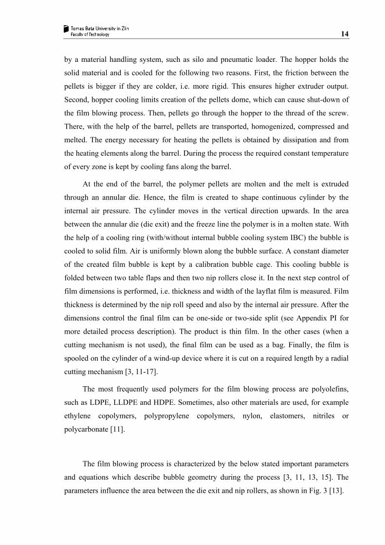
Draw resonance is also called “periodic diameter oscillation” or “hourglassing”, and
can be seen in Fig. 4 [2]. Draw resonance occurs when the draw-down ratio achieves a
critical value. Thus, especially strain hardening causes the instability in the area of high
strain rates (i.e. high take-up ratio). Draw resonance also occurs due to high strain rates in
the case of linear polymers where strain hardening does not exist. In this type of instability,
film width is changed (increases and consequently decreases) at 2 to 10-second intervals
by the internal bubble air. It can also happen if the bubble is perforated or air ring is not
properly adjusted.
This instability can be eliminated by increasing the freeze line height, which can be
controlled by increasing extruder output, higher screw velocity (reduction of the take-up
ratio) and nip rolls speed, or by slower bubble cooling (i.e. modification of the air ring).
Other solutions include increasing melt temperature or using polymer with higher Melt
Index (MI) without strain hardening. Last but not least, stabilization can be done through
narrowing the die gap and take-up ratio reduction.
20
Fig. 4. Draw resonance
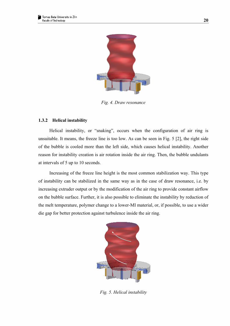
1.3.2 Helical instability
Helical instability, or “snaking”, occurs when the configuration of air ring is
unsuitable. It means, the freeze line is too low. As can be seen in Fig. 5 [2], the right side
of the bubble is cooled more than the left side, which causes helical instability. Another
reason for instability creation is air rotation inside the air ring. Then, the bubble undulants
at intervals of 5 up to 10 seconds.
Increasing of the freeze line height is the most common stabilization way. This type
of instability can be stabilized in the same way as in the case of draw resonance, i.e. by
increasing extruder output or by the modification of the air ring to provide constant airflow
on the bubble surface. Further, it is also possible to eliminate the instability by reduction of
the melt temperature, polymer change to a lower-MI material, or, if possible, to use a wider
die gap for better protection against turbulence inside the air ring.
Fig. 5. Helical instability

21
1.3.3 Instability of the freeze line height (FLH instability)
Another type of instability presents as changing the freeze line height, that is why it
is also called “periodic oscillation of the freeze line height”. The oscillations appear in
30-second to 5-minute intervals. This can be caused by surging, flow of surrounding air, or
relatively slow changes in ambient temperature. Oscillations are in the range of several
centimeters. For the long oscillation times the bubble seems to be stable at first sight
(Fig. 6) [2]. However, in more detail, in the area of freeze line there is a little thickness
variation in the machine direction. It is caused by high internal pressure in the bubble or
changes of the bubble temperature.
As presented above, surging is one of the reasons of the instability creation. Surging
is the result of extruder motor amps and back pressure - the freeze line height rises and
falls. The problem can be solved by lowering the temperature of the extruder feed and
second barrel zones (better feeding and melting). In this context, it is important to avoid
blending polymers with very different melt flow indexes that do not mix well. Then, an
appropriate air ring, haul off speed or unworn screws are necessary for good mixing. Thus,
especially when the freeze line height changes during the film blowing process and it
cannot be eliminated, the bubble is shielded by e.g. a bubble calibration cage.
Fig. 6. FLH instability
1.3.4 Heavy-bubble instability
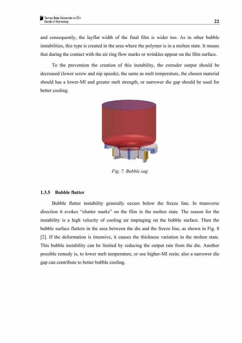
Poor cooling of the bubble creates instability that is called “bubble sag” or “sleeping
bubble” and also “heavy bubble”. In such a case, the bubble can touch the air ring, as
shown in Fig. 7 [2]. This happens when the force of the cooling air is higher than the
tensile strength of the processed material. Then, bubble diameter is bigger than it should be
22
and consequently, the layflat width of the final film is wider too. As in other bubble
instabilities, this type is created in the area where the polymer is in a molten state. It means
that during the contact with the air ring flow marks or wrinkles appear on the film surface.
To the prevention the creation of this instability, the extruder output should be
decreased (lower screw and nip speeds), the same as melt temperature, the chosen material
should has a lower-MI and greater melt strength, or narrower die gap should be used for
better cooling.
Fig. 7. Bubble sag
1.3.5 Bubble flutter
Bubble flutter instability generally occurs below the freeze line. In transverse
direction it evokes “chatter marks” on the film in the molten state. The reason for the
instability is a high velocity of cooling air impinging on the bubble surface. Then the
bubble surface flutters in the area between the die and the freeze line, as shown in Fig. 8
[2]. If the deformation is intensive, it causes the thickness variation in the molten state.
This bubble instability can be limited by reducing the output rate from the die. Another
possible remedy is, to lower melt temperature, or use higher-MI resin; also a narrower die
gap can contribute to better bubble cooling.

23
Fig. 8. Bubble flutter
1.3.6 Bubble breathing
When the internal cooling air changes the bubble volume, the bubble increases and
decreases periodically – the bubble “breathes” (Fig. 9) [3]. In this case, there are
fluctuations in layflat width and machine direction film thickness. The breathing cycles can
be shorter or longer, which depends on the amount of variation or speed of the cycle. This
problem can be solved by reducing melt temperature, using higher-MI resin or decreasing
extruder output. The machinery can be controlled by internal bubble cooling valves,
blowers and sensors. Thus, the internal bubble cooling system plays a very important role
from process stability point of view.
Fig. 9. Bubble breathing
1.3.7 Bubble tear
The “snap off”, which is another term for the bubble tear instability, is created when
the tensile stress at the film blowing exceeds the material strength. It means that the

24
take-off force, F, needed to draw up the bubble is higher than the tensile strength of the
molten film. In such a case, the created bubble is torn in the direction of the acting force
(machine direction) and the bubble tears off from the die exit (Fig. 10) [2]. This happens in
high-molecular-weight polymers that experience high degree of strain hardening at high
draw-down rates. To eliminate the problem, the cooling rate has to be reduced by suitable
adjustment of the air ring. Other solutions are in reduction of extruder output, increase of
the die and melt temperature, using a polymer with a higher melt index (without strain
hardening) or by a narrower die gap, which should reduce the draw-down rate.
Fig. 10. Bubble tear
The above presented bubble instabilities include various problems: from variation of
film thickness and width to scratches and tears. In the process with bubble instabilities it is
very difficult to predict the exit velocity of an individual polymer. Stability of the film
blowing process is influenced by the properties and structure of the polymer, process
variables and design of the air ring [2, 23, 26]. Particularly the design of the air ring is very
important for the determination of maximum exit velocity, i.e. for the definition of bubble
instability. Therefore the study of the bubble stabilization is crucial.

25
1.3.8 The area of stable and unstable bubbles
The correct setting of the film blowing process parameters decides about the bubble
instabilities. The below presented set of graphs, experimentally determined in [27], can be
a useful tool for a technologist with respect to better determination of film blowing
stability region. The graphs show the influence of the mass flow rate, melt temperature and
heat transfer coefficient on the bubble stability under constant other processing conditions.
The effect of mass flow rate (keeping the melt equal to 185oC) on the film blowing
stability is provided in Fig. 11. It is clearly visible that the mass flow rate increase leads to
narrowing of the processing window. Interestingly, this experimental work suggests that at
higher flow rates, the bubble is stable only for BUR > 1 even if the maximum cooling rate
is applied.
0 1 2 30.5 1.5 2.5 3.5
BUR
0
6
12
18
24
30
36
42
48
54
60
66
72
78
84
90
96
102
TUR
Rupture of bubblem = 2.0 kg/hm = 4.5 kg/hm = 6.5 kg/h
STABLE
Draw resonance Helical instability
Increase of mass flow rate
Fig. 11. Effect of mass flow rate on the film blowing stability (LDPE
material, FLH = 250mm, Tmelt = 185oC) [27]. Note that unstable area
occurs below the stability contours.

26
The effect of air cooling efficiency (heat transfer coefficient) on the film blowing
stability based on [27] is depicted in Fig. 12. It is nicely visible that a more efficient
cooling strongly stabilizes the bubble.
0 0.5 1 1.5 2 2.5
BUR
0
6
12
18
24
30
36
42
48
54
60
66
72
78
84
90TU
R
L = 180 mL = 250 m
STABLE
Helical instability
Draw resonance+
FLH instability
Fig. 12. The effect of FLH on the film blowing stability (LLDPE
material, mass flow rate is 2kg/h, Tmelt = 187oC) [27]. Note that
unstable area occurs below the stability contours and vice versa.
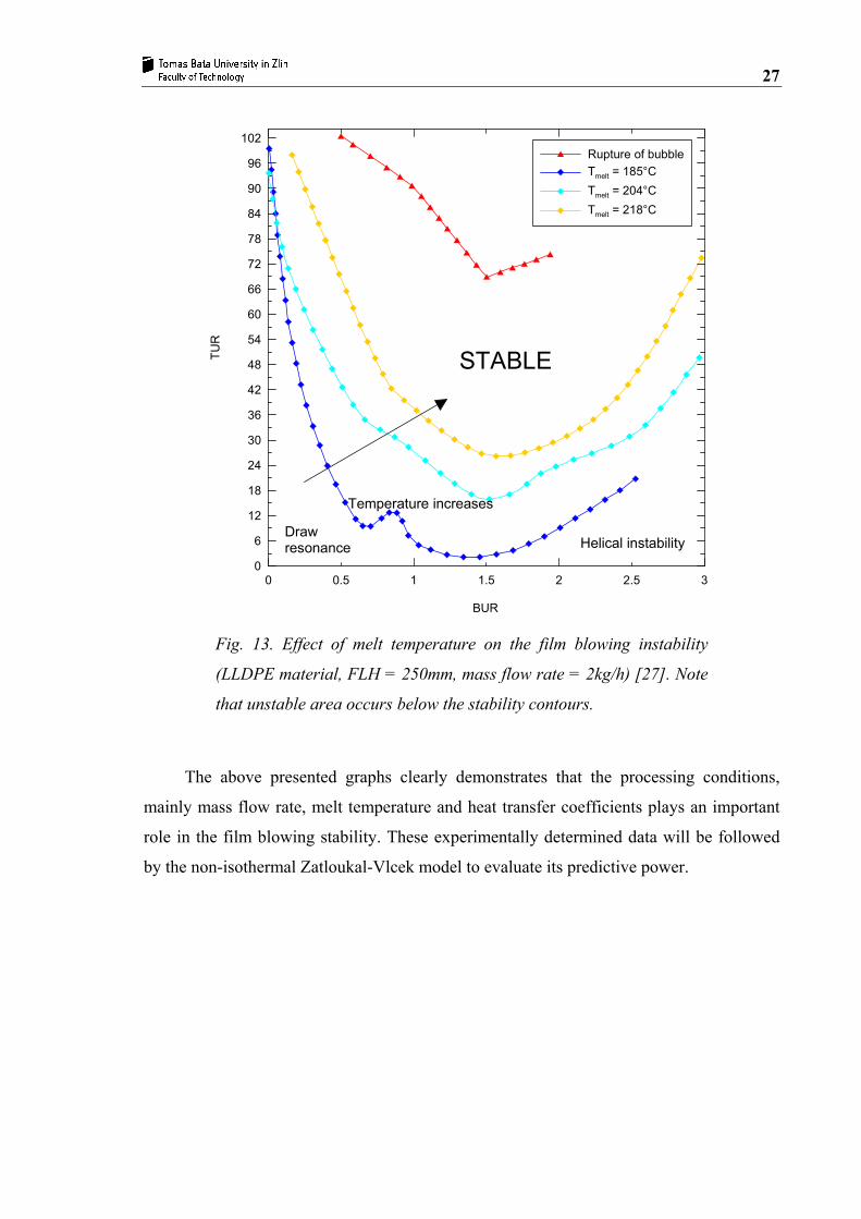
Finally, the effect of melt temperature on the film blowing instability is depicted in
Fig. 13. Clearly, the melt temperature increase leads to decrease in the film blowing
stability and vice versa, which is also in agreement with the observations of Han et al.
[28, 29].
27
0 1 2 30.5 1.5 2.5
BUR
0
6
12
18
24
30
36
42
48
54
60
66
72
78
84
90
96
102
TUR
Rupture of bubbleTmelt = 185°CTmelt = 204°CTmelt = 218°C
STABLE
Draw resonance Helical instability
Temperature increases
Fig. 13. Effect of melt temperature on the film blowing instability
(LLDPE material, FLH = 250mm, mass flow rate = 2kg/h) [27]. Note
that unstable area occurs below the stability contours.
The above presented graphs clearly demonstrates that the processing conditions,
mainly mass flow rate, melt temperature and heat transfer coefficients plays an important
role in the film blowing stability. These experimentally determined data will be followed
by the non-isothermal Zatloukal-Vlcek model to evaluate its predictive power.

28
2 STABILIZATION OF THE FILM BLOWING PROCESS
During the film blowing process the bubble stability is influenced first of all by
cooling of the bubble. For this purpose, an air ring or internal bubble cooling (IBC) system
can be used. The bubble stability is also affected by the mechanical parts, such as iris,
bubble guides and bubble calibration cage. The stabilization methods are presented below
in more detail.
2.1 Bubble stabilization by cooling system (melt area)
The air cooling system (Fig. 14) [30] is a very important part of the film blowing
line. It can be arranged both inside and outside of the bubble, or only outside. Internal
bubble cooling is done with the help of an exhaust pipe. The outside bubble cooling is
affected by an air ring. These types of cooling are used for the following reasons: First,
cooling of the creating bubble is provided to heat removal from the molten polymer film.
Generally, polyethylene has a higher specific heat than other polymers. Then, the material
needs longer distance to cool. Second, it affects the stability of the film blowing process.
Third, bubble cooling has an influence on the bubble forming. Last but not least, bubble
cooling has a fundamental importance for the polymer mass throughput and final film
properties. If the cooling system is not used during the process, the film blowing process
will not work well. [3, 30-32]
Fig. 14. Cooling system
HOT AIR COLD AIR
COLD AIR COLD AIR
HOT AIR
IBC SYSTEM
AIR RING

29
During the bubble cooling, air stream properties are very important for the cooling
effectivity. First, air speed determines the rate of heat removal from the film. The higher
the air speed, the faster the film cooling. However, too fast stream of air causes bubble
instability and the final film has poor properties. Second, air temperature has an influence
on cooling speed. The colder air, the faster the film blowing process can be. On the other
hand, if the cooling air should have a low temperature, the film processing will be too
expensive. In such a case it is necessary to use insulation on the air hoses and air rings due
to moisture condensation. Air temperature around the film blowing line is also very
important. It must be taken into account because the freeze line height changes during the
day and night. In this case, there is a requirement of air condition with the constant air
temperature. Another aspect is air humidity, which affects the cooling effect; higher
humidity leads to better cooling effect and vice versa [3, 31]. However, this opinion is not
uniform, so further research is needed in this area.
As written above, bubble cooling can be realized by an air ring with/without internal
bubble cooling system. This will be described in more detail [3, 31].
2.1.1 External cooling system – air ring
In this system the cooling part of the film blowing line is set on the top of the die,
rather than on the insulating board, which presents insulation between the cool air ring and
hot die. Cooling air is transported by the air ring directly onto the outer bubble surface. The
air is blown through a number of hoses that are connected to the air ring around its
circumference. Then, inside the ring, air flows into a series of baffles. Thus, air flow is
balanced and ready for cooling of the creating bubble by flowing directly onto the outside
of the bubble.
During the film blowing process, constant temperature of the surrounding air is very
important as well as the temperature inside the die. For this purpose an insulating board is
used to separate the two different environments. In an opposite case the film production
efficiency will decrease.
In the film blowing process, it is possible to use two main types of the air ring. These
are single and dual lips. The lip type is chosen first of all according to the bubble shape.

30
The single lip system, presented below in Fig. 15 [3], is used in the case of a stable
bubble, for low-density polyethylene LDPE (low freeze line) or high-density polyethylene,
HDPE (high freeze line). Thus, the single lip system is applicable first of all in the case of
the higher freeze line and for high-melt-strength materials [3, 13, 30].
Fig. 15. Single lip design
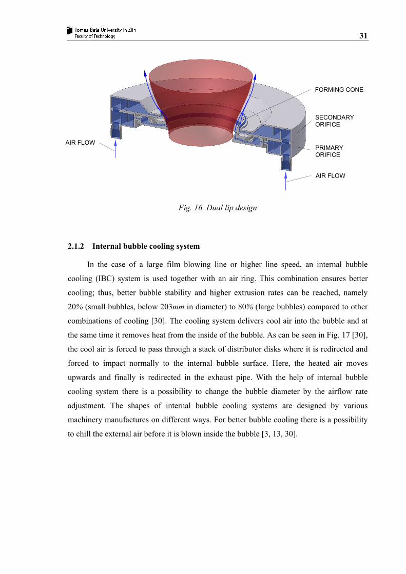
A more expensive air ring type is the dual lip system. The basic design of the dual lip
air ring is in the form of primary and secondary orifices which are separated by forming
cone, as can be seen in Fig. 16 [3]. This cone sets the air flow, bubble shape and volume
ratio in the two orifices. The primary orifice is lower and provides a small volume of air to
the die exit with the view of increased melt strength and, also to prevent the bubble from
touching the cone. Then, the bubble goes around the second orifice, which provides large
volume of air to make solid film bubble. Thus, the length and shape of the cone determine
the second orifice diameter.
The dual lip system is applied for the materials which tend to produce bubble
instabilities, such as linear low-density polyethylene, LLDPE. This system provides not
only cooling of the bubble, but also aerodynamical stabilization and film dimensional
accuracy and is mainly used for low-melt-strength materials with lower freeze line height.
[3, 18, 30].
AIR FLOW
AIR FLOW
31
Fig. 16. Dual lip design
2.1.2 Internal bubble cooling system
In the case of a large film blowing line or higher line speed, an internal bubble
cooling (IBC) system is used together with an air ring. This combination ensures better
cooling; thus, better bubble stability and higher extrusion rates can be reached, namely
20% (small bubbles, below 203mm in diameter) to 80% (large bubbles) compared to other
combinations of cooling [30]. The cooling system delivers cool air into the bubble and at
the same time it removes heat from the inside of the bubble. As can be seen in Fig. 17 [30],
the cool air is forced to pass through a stack of distributor disks where it is redirected and
forced to impact normally to the internal bubble surface. Here, the heated air moves
upwards and finally is redirected in the exhaust pipe. With the help of internal bubble
cooling system there is a possibility to change the bubble diameter by the airflow rate
adjustment. The shapes of internal bubble cooling systems are designed by various
machinery manufactures on different ways. For better bubble cooling there is a possibility
to chill the external air before it is blown inside the bubble [3, 13, 30].
PRIMARY ORIFICE
SECONDARY ORIFICE
FORMING CONE
AIR FLOW
AIR FLOW

32
Fig. 17. IBC system
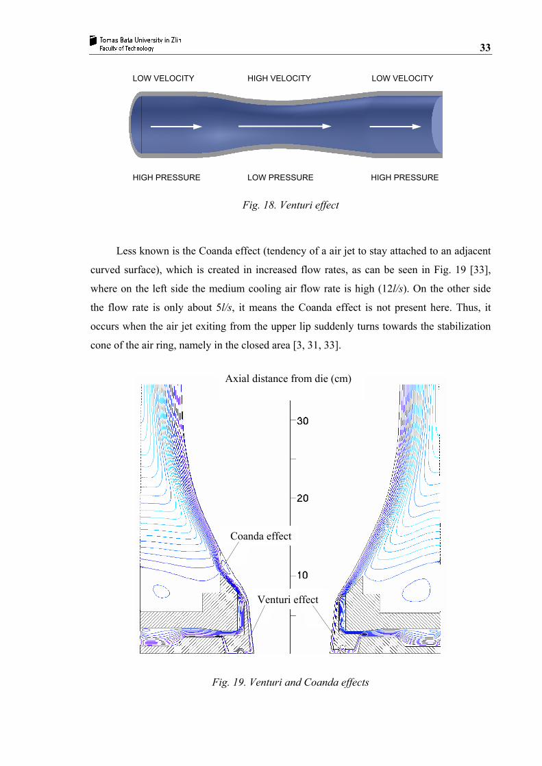
2.1.3 Venturi and Coanda effects
During external cooling of the bubble two important aerodynamic phenomena are
observed - Venturi and Coanda effects. The Venturi effect occurs when air flows through
narrow area where its speed increases and the pressure drops, as can be seen in Fig. 18
[33]. Then, a large vacuum is created near the air ring wall and the melt tube is drawn onto
this wall. So it cools and stabilizes the bubble under the freeze line height and also enables
increased output.
COLD AIR HOT AIR
EXHAUST PIPE
DISTRIBUTOR DISK
33
Fig. 18. Venturi effect
Less known is the Coanda effect (tendency of a air jet to stay attached to an adjacent
curved surface), which is created in increased flow rates, as can be seen in Fig. 19 [33],
where on the left side the medium cooling air flow rate is high (12l/s). On the other side
the flow rate is only about 5l/s, it means the Coanda effect is not present here. Thus, it
occurs when the air jet exiting from the upper lip suddenly turns towards the stabilization
cone of the air ring, namely in the closed area [3, 31, 33].
Fig. 19. Venturi and Coanda effects
HIGH PRESSURE HIGH PRESSURE LOW PRESSURE
LOW VELOCITY LOW VELOCITY HIGH VELOCITY
Axial distance from die (cm)
Coanda effect
Venturi effect

34
Due to the fact that both phenomena may have significant effect on the air flow
character/heat transfer coefficient, they also should be taken into account when film
blowing stability analysis is performed.
2.2 Bubble stabilization by mechanical parts (solid area)
In the film blowing process the solid bubble (i.e. above the freezeline) is usually
stabilized by external devices such, as irises, bubble guides and bubble calibration cages.
The stabilization of the solid bubble is necessary because the bubble is sensitive to side
movements from environmental effects, for example draft. This movement, called
“dancing” is the cause of disunited wall thickness and it occurs in the case of bubbles with
a small diameter and large height. With the use of bubble stabilization the film can be
scratched. It happens when the below presented devices do not work properly [3, 13].
2.2.1 Iris
This stabilization device is set above the air ring, as presented in Fig. 20 [13]. The
construction is very simple and it is very effective. The iris function consists in the change
of the iris diameter according to the blow up ratio. Iris enables to hold the cooling air on
the bubble surface in the area between the die exit and iris. Then the bubble cooling is
more intensive. The problem about using of the iris is in the creation of the bubble rattling,
which is affected by the cooling air volume [3, 13].
Fig. 20. Stabilization by iris
IRIS ADJUSTMENT

35
2.2.2 Bubble guides
Bubble guides are required between the freeze line and table flap to support and
guide solid bubbles in processes with a higher output. Setting of the guides position has to
guarantee concentricity of the bubble to the die. There are two modifications of the bubble
guides (which are usually made from teflon). The first (Fig. 21) [13] is in the form of four
bars which are closed with spur gears. They move towards the bubble with the help of the
chain sheave until they touch it. Rotation around its axis is not allowed [13, 30].
Fig. 21. Bubble guides – type A
CHAIN SHEAVE
FREEZE LINE HEIGHT
COLLAPSER GUIDE
BUBBLE
SPUR GEARS

36
The other type (Fig. 22) [13] has a better construction. There are four cylindrical
arms, each of which can be adjusted. Then, they are in a good contact with the bubble
surface and rotation around its axis is allowed.
Fig. 22. Bubble guides – type B
2.2.3 Bubble calibration cage
Another method to stabilize solid bubble is a bubble cage (Fig. 23) [13]. This device
limits the lateral movement of the bubble and it lowers the bubble tension. The cage,
FREEZE LINE HEIGHT
CYLINDRICAL ARMS
BUBBLE

37
surrounding the film bubble, consists of a frame, arms and segmented rollers. The frame
holds the cage and it provides a possibility to attach IBC sensors, and it also provides
setting of the cage height with regard to variable freeze line height. The bubble cage is
concentric to minimize friction. Then, the dimensions uniformity is better. A bubble cage
is part of every film blowing line [13].
Fig. 23. Bubble calibration cage
ARMS ADJUSTMENT
FREEZE LINE HEIGHT BUBBLE
FRAME
ROLLERS
HEIGHT ADJUSTMENT
VARIABLE SPACING OF ARMS

38
3 MODELING OF THE FILM BLOWING PROCESS
Due to the fact, that film blowing instabilities described above represents the main
limiting factor for this technology, any knowledge leading to their deeper understanding
with respect to material property, die design and processing conditions are very welcome.
Parametric study performed by the use of the film blowing modeling is widely used for
such purpose. In the next section, the film blowing models are summarized and some of
them are discussed in more detail.
3.1 Review of the current models
Tab. 2 summarized different film blowing models in chronological order based on
the open research literature.
Tab. 2. Summary and description of the constitution equations for the solution of the film
blowing process (adapted from [34]).
Author Model description Limitations
Pearson and Petrie [16, 35] Isothermal Newtonian
Does not incorporate the non-Newtonian flow behavior of polymer melts
Petrie [36]
Non-isothermal Newtonian and isothermal purely elastic model. Effects of gravity and inertia included
Does not allow for viscoelas-tic response of materials
Han and Park [37] Isothermal power law Does not account for cooling of bubble and viscoelasticity
Wagner [38] Non-isothermal integral viscoelastic equation with Wagner damping function
Complex, does not accurately estimate stresses at the die exit
Pearson and Gutteridge [39] Non-isothermal elastic model Does not allow for the viscoe-
lastic response of materials
Gupta [40] General non-isothermal White – Metzner equation
Used only for film blowing of PS bubbles
Kanai and White [41] Non-isothermal Newtonian with crystallisation
Does not allow for non-Newtonian behavior of fluids

39
Author Model description Limitations
Luo and Tanner [4] Non-isothermal Maxwell model and Leonov models joined together
Solutions highly unstable, the model does not account for non-linear viscoelasticity
Cain and Denn [42] Marruci model Does not account for multiple relaxation time spectrum
Seo and Wissler [43] Isothermal Newtonian Does not attempt non-Newtonian due to the high Weisenberg effect
Cao and Campbell [44, 45]
Non-isothermal Maxwell model extended above the freeze line with Hookean elastic model
Highly unstable, does not predict creep flow very well
Ashok and Campbell [5]
Maxwell model with a single relaxation time and the Oldroy
Does not allow extrudate swell and temperature gradient across the film
Alaie and Papanastasiou [46]
Non-isothermal integral viscoelastic equation with PSM damping function
Complex, difficult to estimate previous shear history of po-lymer melt, particularly at the die exit
Liu et al. [47]
Quasi cylindrical bubble combined with non-isothermal power law with crystallization effects consti-tutive equation
Does not allow for axial cur-vature of bubble and viscoe-lastic properties of melt
Sidiropoulos et al. [48, 49]
Modified non-isothermal Newtonian
Does not allow for viscoelas-tic nature of polymer melt
Kuijk et al. [50] Comprehensive model for film blowing
Used only for film blowing of PE bubbles
Zatloukal and Vlcek- (variational principles 1) [7]
Isothermal elastic model (Hookean)
Does not account for the flow behavior and the bubble movement
Zatloukal and Vlcek- (variational principles 2) [6] Isothermal Newtonian
Does not incorporate the non-Newtonian flow behavior of polymer melts
Zatloukal and Vlcek- (variational principles 3) [8]
Non-isothermal non-Newtonian
Membrane approximation. Does not account for flow memory

40
It is obvious that many film blowing models are based on the Pearson and Petrie
formulation [1, 16, 35]. The recently proposed film blowing model based on minimum
energy approach and variational principles [6-8] seems to be breakthrough in the film
blowing modeling because it is numerically stable, gives realistic predictions and it can
also be coupled with the Pearson and Petrie formulation, as shown in [6]. Hence, in the
next section the specific attention will be paid only to these two formulations.
3.2 Pearson and Petrie formulation
The first and the most important contribution to modeling of the film blowing
process were given by Pearson and Petrie [1, 2, 11] who developed basic and simple
kinematic frame of the film blowing process. In their pioneering work, they have employed
Newtonian model as the constitutive equation and the process has been assumed to be
isothermal. Pearson and Petrie formulation [1, 2] is based on the following assumptions:
(see Fig. 24 for more details):
Membrane theory: the bubble is described as a thin shell where the film thickness,
h, is much smaller than the bubble radius, r (h << r).
The bubble movement is time steady and symmetrical around the bubble axis.
The surface and inertial stresses are neglected due to their low values.

41
Fig. 24. Film blowing variables
The Pearson and Petrie have used a local Cartesian coordinate system where x1
represents the tangential direction, x2 is the thickness direction, and x3 means the
circumferential direction (Fig. 25).
R0 H0
ΔP
F
r
h
H1 R1
L

42
Fig. 25. Cartesian coordinate system
The Mathematically, Pearson and Petrie formulation is given by the set of equations
provided in Tab. 3.
Tab. 3. A full set of the Pearson and Petrie equations.
Equation type Equation form Equation number
Continuity equation ( ) ( ) ( ) ( )( )xTxvxhxrm ρπ2=& (7)
Density ( )
bwPTR
Tg ′+
=
*
1ρ (8)
Internal bubble pressure tm R
hR
hP 3311 σσ+=Δ (9)
Curvature radius - tangential ( )θcosrRt = (10)
Curvature radius - circumfe-rential ( )θ3
2
2
cos
1
dxrd
Rm−
= (11)
x
y
Θx2
x1
x3
r
x

43
Equation type Equation form Equation number
Term ( )
2
1
1cos
⎟⎠⎞
⎜⎝⎛+
=
dxdr
θ (12)
Force balance ( ) ( )2211 cos2 rrPFrh f −Δ−= πθσπ (13)
Stress 11σ ( ) ( )( )( ) ( ) ( )( )xxhxr
xrrPFx f
θππ
σcos2
22
11
−Δ−= (14)
Tangential stress ( )L11σ at the freeze line height
( )11
11 2 HRFL
πσ = (15)
Stress in the circumferential direction
( ) ( )( )
( )( ) ( )⎟⎟
⎠
⎞⎜⎜⎝
⎛−Δ= x
xRxhP
xhxR
xm
t1133 σσ (16)
Circumferential stress at the freeze line height
( ) PHRL Δ=
1
133σ (17)
Proportion between the total stresses,σ , and the extra stresses, τ
223333
22
221111
0ττσ
σττσ
−==
−= (18)
The meaning of the used symbols is following: x represents particular location at the
bubble, m& is the mass flow rate, r(x) the bubble radius, h(x) the film thickness, v(x) the
film velocity, T(x) the temperature and ρ(T) is the density (which is described below in
more detail), ∆P is the internal bubble pressure, σ11 is the tangential directions of the
stress, Rm is radius curvature, σ33 is circumferential directions of the stress, Rt is radius
curvature , rf is the bubble radius at the freeze line height, F means the take-up force, G
stands for the gravity, and H is the force created by the air flow. The bubble radius at the
freeze line height is, R1 = BURR0, and H1 is the bubble thickness at the same place.
It should be mentioned that Eq. (8) for temperature dependent density has been
derived by Spencer and Gilmore [51] with following symbol meaning: w is the molecular
weight, Rg represents the universal gas constant (Rg = 8.314J·K-1.mol-1), P* is the cohesion
pressure, and b′ means the specific volume. As has been shown by Hellwege et al. [52],

44
these parameters for PEs, takes the following forms: w = 28·10-3kg·mol-1,
b′ = 8.75·10-4m3.kg-1 and P* = 3.18·108Pa. Putting all these numbers into the Eq. (8), the
following equation for temperature dependent density raised:
( )( ) ( ) 875.010934.0103
3
+⋅= − xT
xTρ (19)
Main problem with the Pearson and Petrie formulation is the occurrence of numerical
instabilities [2, 4, 7, 9] and impossibility to represents real bubble shapes realistically [2, 7,
9, 53].
Numerical instabilities
These types of instabilities are usually caused by inability of the numerical scheme to
converge for certain polymer rheology, processing and boundary conditions or by
existence of the multiple solutions. Moreover, the solution is very sensitive to the initial
bubble angle at the die exit as well as to melt history which is related to the die flow. Due
to that, the solution is available for only a small area of the operating conditions. This is
discussed in more detail by Luo and Tanner [4].
Problems with the bubble-shape description
These problems are connected with high stalk bubbles, i.e. bubbles with a long neck.
Here, the bubble shape with the original elongated neck is not described exactly - the
predicted values are set in earlier than the elongated neck of the bubble in reality [2, 7, 9,
53].
The presented problems of Pearson and Petrie formulation can be eliminated by the
application of Zatloukal and Vlcek´s formulation derived through variational principles,
which is described in the following parts in more detail.
3.3 Zatloukal and Vlcek formulation
The Zatloukal and Vlcek formulation regards existence of the stable film blowing
process as a situation which is accordant with minimum energy requirements. If the

45
condition is not fulfilled, the film bubble can be considered as unstable. This variational
principle can be used to derive a model which describes the bubble creation. In more
detail, it is well-known that bubble shape changes during the film blowing process. It
happens due to the internal load, p, and the take-up force, F. The bubble can be thought as
a static flexible membrane. Thus, the thickness is a neglected parameter because the
membrane is very thin [2]. Two bubble shapes can be created. First, the bubble before
deformation (Fig. 26) [2, 7, 9]; here the line element of the membrane is dx, and second,
the bubble after deformation (Fig. 27), where the element length is given by the following
equation [2, 7, 9]:
( ) ( ) dxydxy ⎥⎦⎤
⎢⎣⎡ +≈+ 22 ´
211´1 (20)
It has been shown in [7] that if the constant bubble compliance is assumed, one can
derive the analytical equation for the bubble shape satisfying the minimum-energy
requirements by using variational principles [2].
Fig. 26. Membrane
before deformation
Fig. 27. Membrane
after deformation
This model can be used for different processing conditions, which leads to different
bubble types, as will be discussed bellow in more detail.
R0 y
x
L
0 R0 y
x
L
0
F
p
46
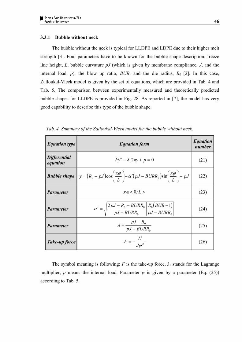
3.3.1 Bubble without neck
The bubble without the neck is typical for LLDPE and LDPE due to their higher melt
strength [3]. Four parameters have to be known for the bubble shape description: freeze
line height, L, bubble curvature pJ (which is given by membrane compliance, J, and the
internal load, p), the blow up ratio, BUR, and the die radius, R0 [2]. In this case,
Zatloukal-Vlcek model is given by the set of equations, which are provided in Tab. 4 and
Tab. 5. The comparison between experimentally measured and theoretically predicted
bubble shapes for LLDPE is provided in Fig. 28. As reported in [7], the model has very
good capability to describe this type of the bubble shape.
Tab. 4. Summary of the Zatloukal-Vlcek model for the bubble without neck.
Equation type Equation form Equation number
Differential equation 021 =+−′′ pyyF πλ (21)
Bubble shape ( ) ( ) pJL
xBURRpJL
xpJRy +⎟⎠⎞
⎜⎝⎛−′−⎟
⎠⎞
⎜⎝⎛−=
ϕαϕ sincos 00 (22)
Parameter >∈< L;x 0 (23)
Parameter ( )
0
0
0
00 12BURRpJ
BURRBURRpJ
BURRRpJ−
−−
−−=′α (24)
Parameter 0
0
BURRpJRpJ
A−
−= (25)
Take-up force 2
2
ϕJLF −= (26)
The symbol meaning is following: F is the take-up force, λ1 stands for the Lagrange
multiplier, p means the internal load. Parameter φ is given by a parameter (Eq. (25))
according to Tab. 5.

47
y (m)
x (m
)
Tab. 5. Parameters A and φ for different bubble shapes (y). Parameters A´, A´´ are
equal to A and parameters φ´, φ´´ are the same as φ [2].
Equation A φ y
1. 1 0 0R
2. 0 < A < 1 ⎟⎟⎠
⎞⎜⎜⎝
⎛ −A
Aarctg21
The form of Eq. (22)
3. 0 π/2 ( )⎭⎬⎫
⎩⎨⎧
−⎟⎠⎞
⎜⎝⎛− BUR
LxR 12
sin10π
4. -1 < A < 0 ⎟⎟⎠
⎞⎜⎜⎝
⎛ −+
AAarctg
21π The form of Eq. (22)
5. -1 π ( )⎭⎬⎫
⎩⎨⎧
+−⎟⎠⎞
⎜⎝⎛+ BURBUR
LxR
1cos12
0 π
The Zatloukal-Vlcek model which is given by Eqs. (15), (17), (22, 24-26), (28-33),
(35), (37) and Tab. 5 will be used in the theoretical part of the Master thesis.
Fig. 28. Bubble without neck [2]. Left
side represents measurements, right
hand side represents prediction.

48
3.3.2 Bubble with neck
A typical material which creates bubbles with the neck is HDPE which is caused by
its extensional strain thinning behavior.
This type of the bubble consist of two sections (Fig. 29) [2, 7]. The first part of the
bubble is influenced by the uniaxial stretching (up to the distance L1) where the radius of
the bubble is changed from R0 to BUR0R0. At the end of the second part of the bubble i.e. at
the freeze line height region, the radius of the bubble is given as BURR0 which is clearly
visible in Fig. 29. In this case, the Zatloukal-Vlcek formulation is given by the set of
equations provided in Tabs. 5-6. The Fig. 30 compares experimentally determined bubble
shape for LLDPE, under processing conditions at which bubble with the neck is created,
and Zatloukal-Vlcek model (see [7] for more detail). Also in this case, the agreement
between model prediction and measured data is very good.
Tab. 6. Zatloukal-Vlcek model for the bubble with the neck.
Equation type Equation form Equation
number
Differential equation 021 =+−′′ pyyF πλ (27)
Bubble shape in section I ( ) ( ) pJ
LxRBURpJ
LxpJRy +⎟⎟
⎠
⎞⎜⎜⎝
⎛ ′′−′′+⎟⎟
⎠
⎞⎜⎜⎝
⎛ ′′−=
100
101 sincos ϕαϕ (28)
Blow up ratio in L1 0
00 2 RpJ
BURRBUR
−= (29)
Parameter ( )
00
00
00
000 12RBURpJ
BURRRBURpJ
RBURRpJ−
−−
−−=′′α (30)
Parameter 00
0
RBURpJRpJ
A−
−=′′ (31)
The neck height L1
( )221 πϕ
ξπϕϕ−′′
−−′′′′=
LL (32)

49
Equation type Equation form Equation
number
Parameter ( )( ) 22200 12 LBURBURpJR −′′−−−= ϕπξ (33)
Tensile force at the die exit J
LFI 2
21
ϕ ′′−= (34)
Bubble shape in section II
( ) ( )⎭⎬⎫
⎩⎨⎧
−⎥⎦
⎤⎢⎣
⎡−
−+= pJR
LLLxpJBURy 0
1
102 cos π (35)
Tensile force at the freeze line height
( )JLLFII 2
21
π−
−= (36)
Internal bub-ble pressure ( )∫ ′+
=Δ L
dxyy
pLp
0
212π
(37)
Surface of the bubble
( )∫ ′+L
dxyy0
212π (38)
Note, that parameter ϕ ′′ is identified with the aid of Tab. 5 according to value A ′′ .
Thus, parameters AA ′′ and ́ are equal to A. The same rule is valid for parameters ϕϕ ′′´, , pL
then represents the force acting at the bubble thickness in the perpendicular direction.

50
x (m
)
y (m)
R 0
BUR 0
R 0
BURR
0
y1
y2
FI
FII
x
y
L1
L
SECTION I SECTION II
Fig. 29. Bubble with neck – shape and acting forces
Fig. 30. Bubble with the neck [2]. Left
side represents measurements, right hand
side represents prediction.

51
3.3.3 High stalk bubble
The term high stalk bubble means that the bubble has an extremely long neck. The
typical material which creates this kind of bubble shape is high molecular weight HDPE.
The thin film which is created by bubble stabilizing equipment at high take-up ratio has
high toughness [6].
This type of the bubble consists of two regions. In Region I the biaxial deformation
is negligible, i.e. the bubble radius can be considered constant. On the other hand, in
Region II the biaxial deformation is considerable due to bubble inflation (see Fig. 31 for
more detail).
For this type of the bubble, Zatloukal-Vlcek model is given by the equations
provided in Tab. 7.
Tab. 7. Zatloukal-Vlcek model for the high stalk bubble.
Equation type Equation form Equation
number
Bubble shape in Region I ( ) ( ) 1
1001
1101 pJ
L´xsinRBURpJ´
L´xcospJRy +⎟⎟
⎠
⎞⎜⎜⎝
⎛−+⎟⎟
⎠
⎞⎜⎜⎝
⎛−=
ϕαϕ (39)
Blow up ratio in L1
122 0
1
022
00 −=
−=
RpJ
RJpBURRBUR '' (40)
Parameter ( )
001
00
001
0001 12RBURpJ
BURRRBURpJ
RBURRpJ'
−−
−−−
=α (41)
Parameter 001
01
RBURpJRpJ
'A−
−= (42)
The neck height L1
( )'
'
JJ'JJ'LJ'
L2
21
2211
1 πϕξπϕϕ
−
−−= (43)
Parameter ( ) 21
22
20200 LJ'JBURBUR'pppBURR −−−−− ⎟
⎠⎞
⎜⎝⎛
⎥⎦⎤
⎢⎣⎡= ϕπξ (44)
Load in Re-gion II 0
222 4 EEpp' π+= (45)

52
Equation type Equation form Equation
number
Membrane compliance in Region II ( )
12
200
22 4
12
−
⎥⎦
⎤⎢⎣
⎡−
+= πE
BUR/BURRp
J'
(46)
Membrane compliance in Region II
222
2 411
πEJ/J '
+= (47)
Bubble shape in Region II
( ) ( )⎭⎬⎫
⎩⎨⎧
−⎥⎦
⎤⎢⎣
⎡−
−+= '''' JpR
LLLxcosJpBURy 220
1
12202
π (48)
Tensile forces ( ) ( )001
2
21 1 BURpRJ'
LFI −+−=
ϕ ( ) ( )00
'2
22
21
'BURBURRp
JLLFII −−
−−=
π (49)
Internal bub-ble pressure ( )∫ ′+
=Δ L
'
dxyy
Lpp
0
2
2
12π
(50)
Here, the J1 is membrane compliance in Region I, and parameter E2 is the Young´s
modulus of the membrane. The total number of the input parameters is six: p, J1, E2, L, R0
and BUR.
Fig. 31. High stalk bubble – shape and acting forces
The comparison between the model prediction and experimentally determined high
stalk bubble shape is depicted in Fig. 32 [6]. Also in this case, the agreement between the
model prediction and measured data is very good.
R 0
BUR 0
R 0 BU
RR0
y1
y2 FI
FII
x
y
L1
L
Region I Region II

53
Fig. 32. High stalk bubble [6]. Left side represents measurements,
right hand side represents prediction.
3.3.4 Stability diagram
In this work, it is considered that the stability diagram is given by three different
stability contours: model contour (above this contour the film blowing process does not
satisfy the minimum energy requirements), machine contour (bellow this contour the
machine direction stress at the freezeline height achieves rupture stress, which leads to
bubble tear) and circumference contour (bellow this contour the circumference direction
stress at the freezeline height achieves rupture stress, which leads to bubble tear). The
mathematical formulas for all three stability contours are summarized Tab. 8. Derivation of
all these equations is provided in [54]. A stable processing window is defined as an area in
the graph of relative final film thickness, H1/H0, vs. BUR. It should be mentioned that the
film blowing process does not satisfy the minimum energy requirements if A < -1.
x (m
)
y (m)

54
Tab. 8. The stability contour equations.
Stability contour Equation title Equation form Equation
number M
odel
stab
ility
con
tour
The membrane compliance
( )BURp
RJ += 1
20 (51)
The extensional rate L
vv DF −=1ε& (52)
The film velocity at the freeze line height and die 102 BURHR
QvF π=
002 HRQvD π
= (53)
The film thickness at the freeze line height
( )( )BURQBURR
pLQBURRHH
+−+
=1
1
002
3200
01 ηππη
(54)
Mac
hine
stre
ss
stab
ility
con
tour
The total stress in machine direction 11011 4 εησ &= (55)
The film thickness at the freeze line height ( )QHRLBUR
QHH
00011
001 2
2ηπσ
η+
= (56)
Cir
cum
fere
nce
stre
ss st
abili
ty
cont
our
The film thickness at the freeze line height
pBURR
H Δ=33
01 σ
(57)
Implicit equation for the BUR definition
( )( )( ) 0
0332
002
0333
121
0 ησϕ
σ−
−−Δ−
=ABURHpBURRRQ
HApL (58)
The symbol description for all above mentioned equations is provided at the end of
this thesis in the List of symbols chapter. It should be mentioned that above mentioned
equations were derived under the assumption that the polymer melt behaves as the
Newtonian fluid and that the film blowing process is isothermal, i.e. freezeline height, L,
has been considered to be one adjustable processing parameter.

55
3.3.5 Energy equation
The assumption about the isothermal film blowing process is relaxed here by
assuming the cross-sectionally average energy equation (the bubble is a quasicylinder at
each point) taken from [55]:
( ) ( )[ ]dxdHv:TTTTh
mR
dxdTC fairBairp
φρτεσρπρ Δ+∇+−+−−= 442& (59)
where Cp stands for the specific heat capacity, ρ is the polymer density, R means the local
bubble radius, h represents the heat transfer coefficient, T is the bubble temperature, Tair
means the air temperature used for the bubble cooling , σB stands for the Stefan-Boltzmann
constant, ε represents the emissivity, τ is the extra stress tensor, ∆v means velocity
gradient tensor, ∆Hf indicates the heat of crystallization per unit mass and φ is the average
absolute degree of crystallinity of the system at the axial position, x.
In order to reduce the problem complexity, the axial conduction, dissipation,
radiation effects and crystallization are neglected. For such simplifying assumptions, the
Eq. (59) is reduced in the following, the simplest version of the cross-sectionally averaged
energy equation:
( )[ ]airp TThydxdTCm −= π2& (60)
where y is the bubble shape (given by Eq. (39) in Tab. 7), m& represents the mass flow rate,
h stands for the heat transfer coefficient, Cp is the specific heat capacity, T means the
value of the bubble temperature and Tair represents the air temperature used for the bubble
cooling. The Eq. (60) applied for the first part of the bubble takes the following form:
( ) ∫∫ =−
LT
T air
p ydxdTTTh
Cmsolid
die 0
2π&
(61)
where Tdie and Tsolid represents the temperature of the melt at the die exit and solidification
temperature of the polymer, respectively. After integration from die temperature, Tdie, up to
freezeline temperature, Tsolid, we can obtain equation defining the relationship between
frezeline height, L, and heat transfer coefficient, h, which take the following simple
analytical expression:
( )( ) ( ) ( ) ( ) ( )( )0002
1BURRcospJcospJsinpJRsinBURRpJhTT
TTlnCmL
airsolid
airdiep ϕαϕαϕϕϕααπ
ϕ+−+−−−⎟⎟
⎠
⎞⎜⎜⎝
⎛
+−−
−−= & (62)

56
With the aim to get equations for the temperature profile along the bubble, it is
necessary to apply the Eq. (60) for any arbitrary point at the bubble i.e. in the following
way:
( ) ∫∫ =−
xT
T air
p ydxdTTTh
Cm
die 0
2π&
(63)
After the integration of Eq. (14), the temperature profile takes the following
analytical expression:
( ) [ ] [ ]⎪⎭
⎪⎬⎫
⎪⎩
⎪⎨⎧
⎟⎟
⎠
⎞
⎜⎜
⎝
⎛+−⎟
⎠
⎞⎜⎝
⎛+⎥
⎦
⎤⎢⎣
⎡−⎟
⎠
⎞⎜⎝
⎛−−−−+=
LxpJpJR
Lxsin
LxcospJBURR
CmLhexpTTTTp
airdieair ϕϕϕαϕ
π00 12
& (64)
3.3.6 Constitutive equations
Constitutive equations represent mathematical relationships which are derived from
constitutive models containing various assumptions and idealizations about the molecular
or structural forces and motions producing stress. Constitutive equations enable computing
polymer melt stress response on the given flow field. Polymers, which lie between
Newtonian liquids and Hookean solids, contain relatively long macromolecules and thus
they cannot be described by simple physical laws [26, 56, 57]
A summary of the various rheological constitutive equations utilized in the film
blowing process modeling is presented above in Tab. 2. As can be seen, a number of
constitutive equations having differential or integral form have already been utilized. In
this work, the recently proposed generalized Newtonian model will be considered [56]
with the aim to minimize the complexity of the problem. The main advantage behind this
model is possibility to express all stress components as the analytical function of
deformation rate even for complex flows where shear and extensional flows are mixed
together. Moreover, specific form of the generalized Newtonian model, described bellow,
allows taking both shear thinning as well as extensional viscosity strain hardening/thinning
behavior properly into account [56]. The model takes the following form:
Dητ 2= (65)
where τ means the extra stress, D represents the deformation rate tensor and η stands for
the viscosity, which is not constant (as in the case of standard Newtonian law), but it is

57
allowed to vary with second, IID, and third, IIID, invariants of deformation rate tensor
according to Eq. (66)
( ) ( ) ( )DIIIfDDD IIIIIII ηη =, (66)
where ( )DIIη and ( )DIII,Tf are given by Eqs. (67-68)
( )( ) ⎟
⎠⎞
⎜⎝⎛ −
⎥⎦⎤
⎢⎣⎡ +
=an
a
Dt
tD
IIa
aII,T
10
21 λ
ηη (67)
( )( ) ξ
β
βα
⎥⎥⎦
⎤
⎢⎢⎣
⎡ +=
)tanh(IIIatanh
III,Tf DtD
3 4 (68)
where η0, λ, a, n, β, α and ξ are adjustable parameters. Note that α is so called extensional
strain hardening parameter. The uniaxial extensional viscosity, needed for model
parameters identification process, is given by the following form:
εττ
η&
yyxxE
−= (69)
where ε& is extensional strain rate.
It should be mentioned that the temperature effect on the polymer melt rheology is
taken into account through shift factor, at, defined through the following well known
Arrhenius equation:
⎥⎦
⎤⎢⎣
⎡⎟⎟⎠
⎞⎜⎜⎝
⎛+
−+
=r
at T.T.R
Eexpa
152731
152731 (70)
where Ea is the activation energy, R is the universal gas constant, Tr is the reference
temperature and T is temperature.
3.3.7 Velocity profile
With the aim to calculate the velocity profile and the film thickness in the
non-isothermal film blowing process, the force balance in vertical direction (gravity and
upward force due to the airflow are neglected) proposed by Pearson and Petrie is
considered in the following form:

58
( )
( )22202
11
'1
2yBURRpF
y
yh−Δ−=
+π
σπ (71)
where 11σ is the total stress in the machine direction and F and pΔ are defined by Eqs. (26)
and (37) in Tab. 4 and Tab. 6. The deformation rate tensor in the bubble forming region
takes the following form:
⎟⎟⎟
⎠
⎞
⎜⎜⎜
⎝
⎛=
3
2
1
000000
εε
ε
&
&
&
D (72)
where the following deformation rate approximations have been used:
L
vvdxdv df −≈=1ε& (73)
LHh
hv
dxdh
hv 0
2−
≈=ε& (74)
( )213 εεε &&& +−= (75)
where v is velocity, vf represents bubble velocity at the freezeline height, vd is bubble
velocity at the die, L is freezeline height, H0 is bubble thickness at the die. Here, v and h
is velocity mean value along the bubble and thickness mean value along the bubble,
respectively, which are defines as follows:
∫=L
dxxvL
v0
)(1 (76)
∫=L
dxxhL
h0
)(1 (77)
Assuming that h << y, then
221111 ττσ −= (78)
By combination of Eqs. (59), (70), (78), the 11σ takes the following form:
⎟⎟⎠
⎞⎜⎜⎝
⎛ ′+= yyv
dxdv2211 ησ (79)

59
After substituting Eq. (79) into Eq. (70), the equation for the bubble velocity in the
following form can be obtained.
( ) ( )[ ]
⎟⎟
⎠
⎞
⎜⎜
⎝
⎛
⎪⎭
⎪⎬⎫
⎪⎩
⎪⎨⎧
−−Δ−+
= ∫L
Tdie dx'y
yaQyBURRpF'y
expvv0
2220
2
21
41
ηπ
(80)
Having the velocity profile, the deformation rates and the thickness can be properly
calculated along the bubble.
3.3.8 Numerical scheme
In order to calculate stability contours for the film blowing process considering
non-isothermal processing conditions and non-Newtonian polymer melt, it is necessary
solved Eqs. (54), (56), (57) as well as implicit function Eq. (58) in Tab. 8. There are two
important points which have to be carefully taken into account. First, the freezeline height
is not adjustable parameter, which becomes constant during the calculation, but its value is
determined by the processing, extrusion design and material parameters through Eq. (62).
Second, the Newtonian viscosity η0 has to be replaced by the representative 'bubble
viscosity - η ' considering average bubble temperature, (Tdie+Tsolid)/2, and components of
the deformation rate tensor through second invariant of deformation rate tensor (see
Eq. 81).
( )23
22
212 εεε &&& ++=DII (81)
For particular processing conditions, iteration loop is needed to get for adjusted
internal bubble pressure particular value of the take-up force which yields a priory known
bubble velocity at the freezeline height. It is considered here, that the representative bubble
viscosity is given by the bubble viscosity at the freezeline. It also has to be pointed out,
that it is considered here that the bubble is characterized by one representative bubble
viscosity value - η ' to get take-up force. However, to take the temperature profile correctly
into account during velocity calculation, representative bubble viscosity is multiplied by
the Arrhenius temperature shift factor in the Eq. (80). Finally, the following procedure has
been used to solve Eq. (58) to obtain circumference stability contour: At the beginning,
parameter A is adjusted to be equal to -1 and corresponding BUR is varied from 0 to 50.
Then, consistent ∆p is calculated. The step in BUR is adaptive to find out the BUR and

60
corresponding ∆p satisfying Eq. (58) for A = -1. Then, the critical film thickness H1 is
calculated by using these two values and Eq. (57). This procedure is repeated for other
values of A, which are varied between -1 and 1 with step 0.05. Of course, Newtonian
viscosity has to be replaced by the representative bubble viscosity for particular
processing/material/die design conditions calculated in the subroutine containing iteration
scheme as described above.

61
4 AIMS OF THE WORK
The main aim of this work is to determine the stability contours (relative final film
thickness vs. BUR) derived from the Zatloukal-Vlcek formulation for a non-isothermal
conditions and non-Newtonian fluids. In more detail, the effect of material properties
(Newtonian viscosity, rupture stress,, index of non-Newtonian behavior, extensional strain
hardening, flow activation energy), process conditions (mass flow rate, heat transfer
coefficient, internal bubble pressure, die exit temperature, cooling air temperature) and die
design (die radius) on the bubble stability will be investigated. The predicted stability
contours and trends will be compared and discussed with the real experimental data.
Specific attention will be paid to the effect of the long chain branching on the stability of
the film blowing process for linear, slightly branched and highly branched LLDPE.
62
II. EXPERIMENTAL

63
5 MATERIAL
In this work, three metallocene based LLDPEs (with chemically identical structure)
having different level of the LCB were considered for the experiments on the film blowing
line. The grades are referred to as mLLDPE low (virtually linear structure), mLLDPE
middle (low level of LCB) and mLLDPE high (high level of LCB). Note, that the
mLLDPE does not have as much LCB as a conventional LDPE. It should be pointed out
that no additional information about these three materials are mentioned in this work
because the institution providing these materials is wishing to keep this information as
confidential.

64
6 FILM BLOWING EXPERIMENT
Pertinent film blowing processing parameters such as internal bubble pressure, Δp,
volumetric flow rate, Q, die gap, H0, bubble radius at the die exit, R0, and freeze line
height, L, were obtained from measurements on the film blowing line depicted in Fig. 33a,
33b in cooperation with Dr. Mike Martyn from Bradford University, UK.
Fig. 33. Film blowing experimental set-up. 33a) General view of the experimental film
blowing line; 33b) Closer view of the film blowing die; 33c) Used spiral mandrel.
The processing equipment comprised of a Betol BC 38mm single screw extruder
equipped with a Davis Standard model DSBMT barrier screw and spiral mandrel die
(Fig. 33c) having six feeding channels. The die annulus was 74mm in diameter and had a
gap equal to 1.34mm. In-house software has been developed to measure the profile of the
bubble. Bubble images taken with a Pulnix PEC 2010 CCD camera are captured using a
bt878 based capture card. The edges of the bubble are determined by a simple thresholding
technique. As no easily locatable features exist on the film to enable scaling, the
33a 33b
2c
33c

65
dimensions of the bubble are determined following a calibration stage that identifies the
positions of four Light Emitting Diodes (LEDs). The basic point of the experimental work
was the determination of the processing window for linear and branched mLLDPEs. The
main experimental results are depicted in Fig. 34 where the experimentally determined
stability diagrams (relative film thickness at the freeze line vs. BUR) for linear and
branched mLLDPEs are provided.
Fig. 34. The experimentally determined stability contours for both, linear and branched
metallocene LLDPE samples (FLH 180mm and temperature 190°C).
The lines superimposed on Fig. 34 demark areas of stable and unstable bubble. The
areas above the lines are stable, while those below the lines are regions of bubble
instability. The experimental data clearly show that the branched mLLDPEs are much
more stable compared to linear melts, i.e. branched mLLDPEs can be used to produce
thinner film at a higher BUR. More importantly, these experimental results suggest that
processibility of the mLLDPEs in film blowing process can be improved by increasing the
content of LCB up to an optimum level. Increasing the LCB content beyond this level
narrows the processing window for stable film production. These experimental data were
taken as a basic for the testing of the recently proposed Zatloukal-Vlcek film blowing
model. All three tested mLLDPEs were carefully characterized by Jan Musil Bachelor
thesis [57] from the rheological point of view. In more detail, the frequency dependent
1 1.2 1.4 1.6 1.8 2 2.2 2.4 2.6 2.8 3 3.2
BUR
0
0.005
0.01
0.015
0.02
0.025
0.03
0.035
0.04
0.045
0.05
0.055
0.06
H1 /
H0
Linear mLLDPEMiddle mLLDPEHigh mLLDPE
STABLE
UNSTABLE

66
linear viscoleastic properties (storage modulus G’, loss modulus G’’), of these three
materials were measured with use of the Advanced Rheometric Expansion System (ARES
2000) Rheometrics rheometer. The transient uniaxial extensional viscosity of each melt
was measured using the ARES 2000 rheometer equipped with the SER Universal Testing
Platform (SER-HV-A01 model) from Xpansion Instruments [7]. The comparison between
frequency dependent complex viscosity for all three samples is given in Fig. 35a. Clearly,
the increase in the LCB slightly increases the Newtonian viscosity, however, at higher
shear rates the viscosity for all three materials becomes almost identical. Finally, the
extensional data in Fig. 35b clearly shows that increase in the LCB leads to strain
hardening behavior leading to higher melt strength.
Fig. 35. Rheology data for tested resins taken from [57]; 35a) Complex viscosity data for
three mLLDPEs having different levels of long chain branching obtained experimentally
by ARES rotational rheometer at 140oC; 35b) Time-dependent uniaxial extensional
viscosity ( )tE+η data for three mLLDPEs having different levels of long chain branching
obtained by SER at 140oC.
10-2 10-1 100 101
Time (s)
101
102
103
104
105
106
107
η Ε+ (t,
ε 0) (
Pa.
s)
mLLDPE lowmLLDPE middlemLLDPE high
mLLDPE low, mLLDPE middle, mLLDPE high at 140°C
ε0 = 20s-1
ε0 = 10s-1ε0 = 3.16s-1
ε0 = 1s-1
1 10-1 100 101 102
Frequency (rad.s-1)
104
2x10⁴
3x10⁴
9x10³
8x10³
7x10³
6x10³
5x10³
4x10³
Com
plex
vis
cosi
ty (P
a.s)
mLLDPE lowmLLDPE middlemLLDPE high
mLLDPE low, mLLDPE middle, mLLDPE high at 140°C35a 35b

67
RESULTS AND DISCUSSION
Theoretical film blowing stability analysis
The film blowing process stability has been theoretically analyzed by using above
mentioned Zatloukal-Vlcek formulation considering particular processing and materials
parameters summarized in Tab. 9. In more detail, all processing/material parameters were
kept as constants whereas one chosen processing or material parameter was varied with the
aim to reveal its impact on the film blowing stability window. In order to do theoretical
analysis, it was crucially important to prepare suitable C++ program to apply both, iterative
numerical schemes combined by the Regula Falsi method to achieve solution of particular
stability contours.
Tab. 9. Zatloukal-Vlcek model parameters used in the model testing on the Tas's Ph.D.
thesis data for LDPE.
Zatloukal-Vlcek film blowing model parameters
η0
(Pa.s) m&
(kg.h-1) Δp
(Pa) σ
(MPa) R0 (m)
H0
(m)
23809.6 4.20 108 0.800 0.0196 0.0008
Parameters of the generalized Newtonian constitutive equation
a (-)
n (-)
α (s)
β (-)
λ (s)
ξ (-)
0.83 0.34 0.00001 8.12409.10-8 2.78 0.034289
Temperature parameters
TAIR
(°C) TSOLID
(°C) TDIE
(°C) TR
(°C) h
(W.m-2.K-1)Ea
(J.mol-1) R
(J·K-1·mol-1) Cp
(J.kg-1.K-1)
25 96 175 190 49.18 66000 8.314 2300
Zatloukal-Vlcek film blowing model test
At the beginning of the research, it is necessary to check, whether Zatloukal-Vlcek
non-isothermal model for non-Newtonian polymer melts has capability to described

68
experimental reality with respect to bubble shape, velocity and temperature profiles. For
the film blowing model test, experimental data for LDPE provided in the Tas's Ph.D. thesis
[1] were used. As the first step, the rheological characteristic of the LDPE material taken
from [1] were fitted by the generalized Newtonian model (Eq. 66). Fig. 36 clearly shows
that the used generalized Newtonian model can describe extensional as well as shear
viscosity data very well. All model, LDPE material and processing parameters for chosen
processing conditions are summarized in Tab. 9.
Figs. 37-39 compare the calculated bubble shape, velocity and temperature profiles
by using Zatloukal-Vlcek model. It is clearly visible that the bubble shape as well as veloc-
ity profile is in reasonable good agreement with the experimental data. The comparison
between calculated and measured temperature profile reveals that even if the model predict
proper trend, the discrepancy between theoretical and experimental data is high. This can
be caused by the absence of the crystallization term in the energy equation. Moreover, by
neglecting of temperature profile for the velocity profile calculation, may indeed leads to
extremely high deviation between experimental reality and theoretical predictions as indi-
cated in Fig 38. On the other hand by slight adjustment of the flow activation energy and
die/solid temperature leads to much better agreement between measured and predicted
velocity/temperature profile (see Fig. 38 and Fig. 39). Therefore, it can be concluded that
the non-isothermal, non-Newtonian Zatloukal-Vlcek model may represent experimental
reality reasonably and thus can be used for serious film blowing stability analysis.
It should be mentioned that the theoretical analysis of the film blowing model will be
done with the processing/material parameters, which are summarized in Tab. 9 (except of
Newtonian viscosity which will be equal to 200kPa.s with the aim to emphasize particular
stability contours details more properly).
Effect of Newtonian viscosity on the film blowing stability
Predicted effect of the Newtonian viscosity on the film blowing stability is depicted
in Fig. 41. Clearly, increase in the Newtonian viscosity from η0 = 50kPa.s up to about
η0 = 200kPa.s leads to the increase of the film blowing processing window. In more detail,
if Newtonian viscosity increases in this range, the film blowing process becomes more
stable at lower BUR (the minimum achievable film thickness is not influenced by the
Newtonian viscosity in this case) and higher film thicknesses can be reached. On the other

69
hand, continues Newtonian viscosity increase above 200kPa.s does not seem to yield wider
film blowing processing window. In this case, continues Newtonian viscosity increase
above 200kPa.s causes higher film blowing process stability at low BUR for higher film
thicknesses (which wider processing window at higher thicknesses similarly to low
Newtonian viscosity range) but simultaneously blowing stability window is narrowing at
small thicknesses. This interesting finding suggests that the relationship between
Newtonian viscosity and film blowing stability has no monotonic character suggesting
existence optimum value of Newtonian viscosity (or Mw) for needed BUR and particular
final film thickness. All calculated parameters for this specific analysis are provided in
Tab. 10.
Effect of heat transfer coefficient on the film blowing stability
Predicted effect of the heat transfer coefficient on the film blowing stability is visible
in Fig. 42. In this case, low intensity bubble cooling (low heat transfer coefficient) leads to
very narrow processing window whereas the increasing cooling intensity (heat transfer
coefficient increases) causes wider processing window. This theoretical conclusion is in
good agreement with open literature [27]. Interestingly, even if the cooling rate is small
and processing window is very narrow in this case, it is possible to get much thinner final
film thickness in comparison with high cooling rate condition at which so low final film
thicknesses are not achievable. On the other hand, the obtained results suggest that for
heavy-duty bags production (thick final film thickness is required) highly effective cooling
system has to be utilized and thus one should take the cooling efficiency of the film
blowing line properly into account. All calculated parameters for this specific analysis are
provided in Tab. 11.
Effect of internal bubble pressure on the film blowing stability
Predicted effect of the internal bubble pressure on the film blowing stability is visible
in Fig. 43. Clearly, internal bubble pressure increase leads to processing window
narrowing and vice versa. In more detail, internal bubble decrease leads to higher stability
especially at low BUR and high final film thicknesses. Interestingly, stability diagrams
reported in this thesis are usually composed by two contours only (model and machine
contours), which indicates machine stress dominance in comparison with circumference
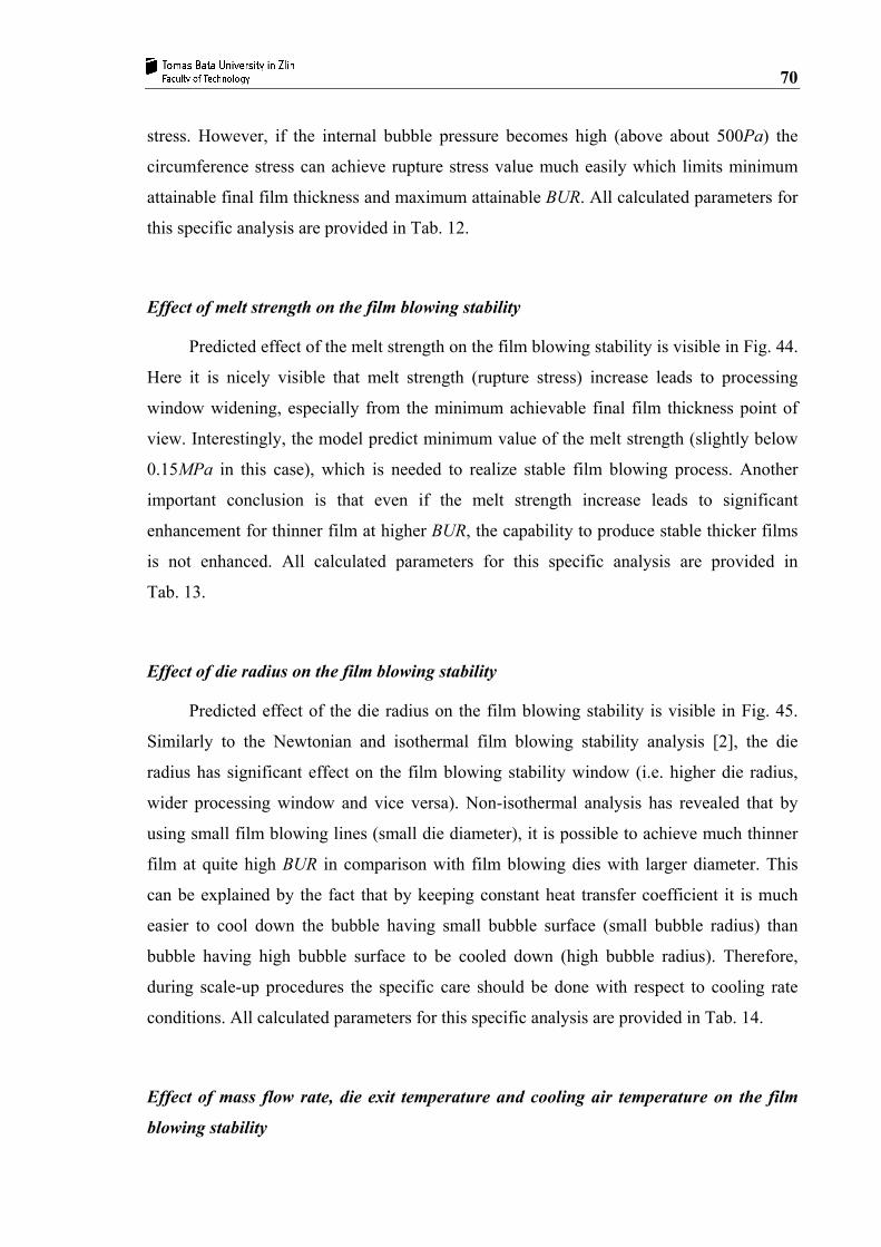
70
stress. However, if the internal bubble pressure becomes high (above about 500Pa) the
circumference stress can achieve rupture stress value much easily which limits minimum
attainable final film thickness and maximum attainable BUR. All calculated parameters for
this specific analysis are provided in Tab. 12.
Effect of melt strength on the film blowing stability
Predicted effect of the melt strength on the film blowing stability is visible in Fig. 44.
Here it is nicely visible that melt strength (rupture stress) increase leads to processing
window widening, especially from the minimum achievable final film thickness point of
view. Interestingly, the model predict minimum value of the melt strength (slightly below
0.15MPa in this case), which is needed to realize stable film blowing process. Another
important conclusion is that even if the melt strength increase leads to significant
enhancement for thinner film at higher BUR, the capability to produce stable thicker films
is not enhanced. All calculated parameters for this specific analysis are provided in
Tab. 13.
Effect of die radius on the film blowing stability
Predicted effect of the die radius on the film blowing stability is visible in Fig. 45.
Similarly to the Newtonian and isothermal film blowing stability analysis [2], the die
radius has significant effect on the film blowing stability window (i.e. higher die radius,
wider processing window and vice versa). Non-isothermal analysis has revealed that by
using small film blowing lines (small die diameter), it is possible to achieve much thinner
film at quite high BUR in comparison with film blowing dies with larger diameter. This
can be explained by the fact that by keeping constant heat transfer coefficient it is much
easier to cool down the bubble having small bubble surface (small bubble radius) than
bubble having high bubble surface to be cooled down (high bubble radius). Therefore,
during scale-up procedures the specific care should be done with respect to cooling rate
conditions. All calculated parameters for this specific analysis are provided in Tab. 14.
Effect of mass flow rate, die exit temperature and cooling air temperature on the film
blowing stability

71
Predicted effect of mass flow rate, die exit temperature and cooling air temperature
on the film blowing stability is visible in Figs. 46-48. Here, increase in die exit temperature
(melt temperature leaving the die) or mass flow rate or cooling air temperature always
causes reduction of the film blowing stability window, which is in agreement with the open
literature [27]. This theoretically obtained observation can be understood thought reduced
cooling efficiency if all the above mentioned investigated variables are increased. Detailed
analysis of these figures reveals that there are slight differences if one compares the
processing window narrowing for cooling efficiency reduction. In all three cases,
increase in these variables leads to reduction of maximum achievable final film thickness
but only for die/melt/cooling air temperature increase, slight improvement in the minimum
achievable final film thickness can be obtained at specific BUR, which can be attributed by
complex melt rheology changes caused by complex thermal history. All calculated
parameters for these specific analyses are provided in Tabs. 15-17.
Effect of power law index (index of non-Newtonian flow behavior) on the film blowing
stability
Predicted effect of the power law index on the film blowing stability is visible in
Fig. 49. Based on the data provided in this figure it can be concluded that decrease in the
power law index causes widening of the film blowing stability window. Closer analysis of
these data led us to the conclusion that the power index increase leads to thinner stable
films and vice versa. This conclusion is in good agreement with the experimental work
reported by Carreau [27] the order for bubble stability has been found to LDPE
(Mw/Mn = 5.2 i.e. power law index is low) > LLDPE (Mw/Mn = 3.8 i.e. power law is
medium) > mLLDPE (Mw/Mn = 2.4 i.e. power law is high - closed to 1). All calculated
parameters for this specific analysis are provided in Tab. 18.
Effect of activation energy on the film blowing stability
Predicted effect of the power law index on the film blowing stability is visible in
Fig. 50. It clearly visible that increase in the flow activation energy leads to slight
widening of the film blowing stability window. This conclusion can be supported by the
experimental work in [27] where it has been clearly demonstrated that film blowing
process is more stable for high flow activation energy LDPE in comparison with low

72
activation energy LLDPE polymer. All calculated parameters for this specific analysis are
provided in Tab. 18.
Effect of Mw on the film blowing stability
The effect of the Mw on the film blowing stability was investigated theoretically by
using three virtual materials by using the generalized Newtonian model where model
parameters were adjusted with the aim to have different level of η0, λ (which corresponds
with Mw increase) and specific flow viscosity curves as depicted in Fig. 51. The results of
the theoretically predicted film blowing stability contours for the fixed processing
conditions and all three virtual materials are summarized in Tabs. 20-21 and Fig. 52. It is
nicely visible that bubble becomes more stable for Mw increase which is in good
correspondence with experimental reality reported in open literature [58]. Note, that in this
case, the freezeline height has been fixed and it has been assumed that all bubbles can
efficiently cooled down (ideal cooling was assumed). Surprisingly, the non-monotonic
trend between Mw increase and the bubble stability has not been found which suggest that
cooling efficiency has strong impact on the film blowing stability.
Comparison between experimental and theoretical film blowing stability
analysis
With the aim to minimize the problem complexity, ideal cooling efficiency was
assumed i.e. it was possible to fix freezeline height for all experiments.
Effect of long chain branching on the film blowing stability
Different type and level of the long chain branching has been theoretically
introduced into different virtual materials through the parameters α and ξ in the
generalized Newtonian model which leads to the different shape of the strain hardening
occurrence in the uniaxial viscosity curve (see Fig. 53 and Fig. 55). Clearly, by comparing
the extensional viscosity curves (Fig. 53 and Fig. 55) and corresponding calculated film
blowing stability contours (Fig. 54 and Fig. 56) the relationship between level of the strain

73
hardening (level of LCB) and bubble stability is non-monotonic which indicates that there
exists optimum level of the LCB. With the aim to explore this point in more detail (with
inclusion of the melt strength), the experimentally determined stability contour lines for
linear as well as slightly and highly branched mLLDPEs (see experimental part for more
detail) were treated numerically. In more detail, the Newtonian viscosity of the melt has
been kept as a constant for all samples in the model whereas melt strength together with
generalized Newtonian model parameters (λ, a, n, α, β, ξ) were varied to find out the
agreement with the experimentally determined stability contours. Fig. 57 shows the
obtained general Newtonian model predictions for linear as well as slightly and highly
branched mLLDPEs. The comparison between the measured and fitted stability contours
are depicted in Fig. 58. The theoretical results in this Figure shows that continued increase
in the melt strength makes the processing window wider, however, the processing window
becomes much narrower with increase in level of LCB in mLLDPE beyond the optimum
LCB level. Clearly, LCB increases not only melt strength but also melt extensional strain
hardening which causes easier stress rise in the film bubble during the processing i.e. at
low LCB level the melt strength increase becomes more effective that extensional viscosity
increase and the bubble may become more stable. However, if the LCB is increased too
much, the strain hardening can become more effective than corresponding melt strength
increase which can not longer compensate the corresponding stress rise and the bubble
becomes more easily unstable

74
CONCLUSION
1. It has been shown that the use of the generalized Newtonian model in the
non-isothermal modeling of the film blowing process together wit Zatloukal-Vlcek
model can be used to investigate the role of processing conditions, machinery design
parameters and polymer rheology from the film blowing stability point of view.
2. It has been theoretically revealed that relationship between Newtonian viscosity
and film blowing stability has no monotonic character suggesting existence optimum
value of Newtonian viscosity (or Mw) for needed BUR and particular final film
thickness.
3. Based on the theoretical stability analysis it has been found that following
processing/material changes have stabilizing effect on the film blowing process:
• Cooling intensity increase
• Internal bubble decrease
• Melt strength increase
• Decrease in the exit temperature (melt temperature leaving the die) or mass
flow rate or cooling air temperature
• Decrease in the index of non-Newtonian flow behavior
• Flow activation increase
It should be mentioned that all above mentioned theoretical conclusion has been
found to be in good agreement with the open literature.
4. It has been shown theoretically, that there is non-monotonic dependence between
extensional strain hardening and bubble stability, which has been found to be in good
correspondence with experimental data.

75
Tab. 10. Summarization of the calculated data in the Fig. 41 for Newtonian viscosity
effect analysis (Q = 15.09168·10-7 m3·s-1).
Point BUR (-)
H1/H0
(-)
L (m)
Δp (Pa)
p (Pa.m)
vF
( m·s-1 ) F
(N) η
(kPa.s) σ11
(MPa) σ33
(MPa)
η 0 =
400
kPa
. s A1 0.840 0.26198 0.35244 108 12.30 0.06907 254.01 1312.509 11.715815 0.008484
B1 1.844 0.39714 0.22925 108 18.91 0.02090 74.51 1024.073 1.032718 0.012286
C1
4.130 0.10680 0.12783 108 33.91 0.03486 406.26 1309.566 9.348471 0.102318
4.130 0.10685 0.12874 1600 498.85 0.05494 423.51 1314.422 9.740942 1.515176
η 0 =
300
kPa
. s A2 1.015 0.18089 0.31042 108 13.96 0.08086 230.64 948.318 12.750244 0.014847
B2 1.994 0.35281 0.21775 108 19.90 0.02179 70.01 793.404 1.010089 0.014954
C2 4.700 0.07949 0.11436 108 37.90 0.04102 328.26 890.399 8.917394 0.156434
4.700 0.07949 0.11562 1700 590.16 0.06103 360.01 897.443 9.779904 2.463171
η 0 =
200
kPa
. s A3 1.400 0.09238 0.27162 108 15.95 0.11835 175.26 566.912 13.754395 0.040099
B3 2.253 0.29393 0.20039 108 21.63 0.02314 62.01 542.850 0.950450 0.020282
C3 5.400 0.04960 0.10185 108 42.56 0.05720 222.26 487.619 8.421339 0.288020
5.400 0.04960 0.10233 1550 632.28 0.07652 272.35 515.256 10.319228 4.133625
η 0 =
100
kPa
. s A4 2.423 0.07304 0.19173 108 22.61 0.03854 64.19 266.379 3.681370 0.087774
B4 2.873 0.19781 0.17268 108 24.83 0.02734 49.95 267.038 0.892116 0.038430
C4 5.400 0.04960 0.09853 108 45.35 0.03349 121.68 267.012 4.610405 0.288020
5.400 0.04960 0.10065 570 241.25 0.03825 109.35 235.365 4.143226 1.520774
η 0 =
50
kPa. s
A5 3.412 0.50851 0.14773 108 29.34 0.06765 41.16 94.949 0.240791 0.017754
B5 3.720 0.12956 0.13888 108 31.21 0.03223 33.26 116.384 0.700426 0.075970
C5 5.400 0.04960 0.07568 108 51.59 0.05059 58.65 110.896 2.222224 0.288020
5.400 0.04960 0.07056 280 95.36 0.05389 51.23 100.380 1.941083 0.746853

76
Tab. 11. Summarization of the calculated data in the Fig. 42 for the heat transfer effect
analysis (Q = 15.09168·10-7 m3·s-1).
Point BUR (-)
H1/H0
(-)
L (m)
Δp (Pa)
p (Pa.m)
vF
( m·s-1 ) F
(N) η
(kPa.s) σ11
(MPa) σ33
(MPa)
h =
70 W
. m-2
. K-1
A1 0.674 0.20206 0.27390 108 11.30 0.11113 191.01 571.949 14.235641 0.008826
B1 1.694 0.44831 0.17286 108 17.91 0.02015 41.51 488.648 0.554789 0.009998
C1
4.500 0.06882 0.08466 108 36.57 0.04946 255.26 496.773 8.365255 0.172996
4.500 0.06882 0.08865 2350 643.25 0.09505 289.65 547.911 9.492543 3.765217
h =
60
W. m
-2. K
-1 A2 0.969 0.13797 0.27593 108 13.09 0.11466 183.76 552.321 13.950553 0.018582
B2 1.953 0.36488 0.18395 108 19.63 0.02147 51.51 517.947 0.733683 0.014162
C2 5.000 0.05879 0.09054 108 39.90 0.05209 237.89 492.600 8.213719 0.225019
5.000 0.05879 0.09156 1800 683.56 0.08189 284.56 520.734 9.825614 3.751677
h =
50
W. m
-2. K
-1 A3 1.400 0.09238 0.27162 108 15.95 0.11835 175.26 566.912 13.754395 0.040099
B3 2.253 0.29393 0.20039 108 21.63 0.02314 62.01 542.850 0.950450 0.020282
C3 5.400 0.04960 0.10185 108 42.56 0.05720 222.26 487.619 8.421339 0.288020
5.400 0.04960 0.10233 1550 632.28 0.07652 272.35 515.256 10.319228 4.133625
h =
40 W
. m-2
. K-1
A4 2.010 0.06156 0.27219 108 19.90 0.12354 163.82 503.359 13.437707 0.086391
B4 2.694 0.21299 0.22060 108 24.56 0.02669 80.26 573.630 1.419732 0.033467
C4 5.930 0.04031 0.11758 108 46.08 0.06409 204.19 482.332 8.670008 0.389233
5.930 0.04031 0.11256 988 395.45 0.07032 228.65 523.564 9.708592 3.561594
h =
30
W. m
-2. K
-1 A5 3.100 0.04042 0.26499 108 27.26 0.12495 153.68 485.213 12.446199 0.202889
B5 3.675 0.13916 0.23232 108 31.09 0.02992 94.26 592.092 1.870756 0.069875
C5 6.500 0.03200 0.15812 108 53.56 0.06325 201.05 472.564 9.810728 0.537452
6.500 0.03200 0.14923 680 286.55 0.06854 156.21 605.653 7.622650 3.387191

77
Tab. 12. Summarization of the calculated data in the Fig. 43 for the internal bubble
pressure analysis (Q = 15.09168·10-7 m3·s-1).
Point BUR (-)
H1/H0
(-)
L (m)
Δp (Pa)
p (Pa.m)
vF
( m·s-1 ) F
(N) η
(kPa.s) σ11
(MPa) σ33
(MPa)
Δp =
50
Pa
A1 0.805 0.13000 0.36216 50 5.54 0.14720 159.26 549.711 15.446551 0.007585
B1 1.843 0.39843 0.22974 50 8.74 0.02089 34.76 479.320 0.480476 0.005666
C1
5.500 0.04922 0.10029 50 20.01 0.05653 219.26 487.649 8.221420 0.136891
5.500 0.04922 0.09892 292 632.46 0.05985 281.45 502.245 10.553309 0.800402
Δp =
100
Pa
A2 1.325 0.09492 0.28038 100 14.32 0.11629 172.07 535.515 13.886618 0.034199
B2 2.194 0.30372 0.20411 100 19.66 0.02300 59.26 537.665 0.902651 0.017698
C2 5.500 0.04922 0.09877 100 40.64 0.05655 220.89 487.702 8.282539 0.273782
5.500 0.04922 0.09892 292 632.46 0.05985 281.45 502.245 10.553309 0.800402
Δp =
200
Pa
A3 2.000 0.07656 0.21729 200 36.95 0.10262 191.48 508.861 12.692540 0.127999
B3 2.694 0.22302 0.17648 200 45.49 0.02551 94.26 580.454 1.592422 0.059190
C3 5.500 0.04922 0.10029 200 80.04 0.05642 223.91 488.293 8.395777 0.547564
5.500 0.04922 0.09892 292 632.46 0.05985 281.45 502.245 10.553309 0.800402
Δp =
300
Pa
A4 2.475 0.06880 0.18759 300 64.19 0.09115 203.32 502.222 12.120191 0.264419
B4 3.056 0.18240 0.16071 300 74.93 0.02750 121.01 593.673 2.203569 0.123147
C4 5.500 0.04922 0.10029 300 120.06 0.05641 227.14 488.539 8.516890 0.821346
5.500 0.04922 0.09892 292 632.46 0.05985 281.45 502.245 10.553309 0.800402
Δp =
400
Pa
A5 2.851 0.06456 0.16932 400 94.82 0.07821 210.19 509.362 11.591838 0.432799
B5 3.335 0.15500 0.15182 400 105.76 0.03037 146.01 595.461 2.866991 0.210857
C5 5.500 0.04922 0.10029 400 160.08 0.05653 230.26 488.929 8.633878 1.095128
5.500 0.04922 0.09892 292 632.46 0.05985 281.45 502.245 10.553309 0.800402
Δp =
500
Pa
A6 3.181 0.06158 0.15591 500 128.74 0.07661 219.14 499.524 11.354953 0.632780
B6 3.594 0.13662 0.14191 500 141.44 0.03120 160.51 592.527 3.318178 0.322267
C6 4.859 0.07430 0.09675 500 207.43 0.04180 212.14 497.495 5.964240 0.801103
4.859 0.07430 0.11119 1200 433.20 0.04331 234.86 538.770 6.603004 1.922679
D6 3.750 0.05725 0.12328 500 162.81 0.06773 237.82 471.575 11.243867 0.802402
Δp =
700
Pa
A7 3.768 0.08079 0.13671 700 205.52 0.05031 215.76 542.233 7.194457 0.799906
B7 4.044 0.11156 0.12924 700 217.41 0.03393 186.51 580.887 4.196316 0.621697
C7 4.358 0.09343 0.11328 700 248.04 0.03764 214.14 548.252 5.338014 0.799920
4.358 0.09343 0.12152 901 296.532 0.05906 211.56 560.164 5.273701 1.029062

78
Tab. 13. Summarization of the calculated data in the Fig. 44 for the melt strength/melt
rupture effect analysis (Q = 15.09168·10-7 m3·s-1).
Point BUR (-)
H1/H0
(-)
L (m)
Δp (Pa)
p (Pa.m)
vF
( m·s-1 ) F
(N) η
(kPa.s) σ11
(MPa) σ33
(MPa)
σ =
1.00
MPa
A1 1.430 0.06938 0.26075 108 18.47 0.12469 216.58 482.325 22.159165 0.054541
B1 2.253 0.29392 0.20039 108 21.63 0.02314 62.01 542.851 0.950479 0.020282
C1
5.600 0.03922 0.01002 108 44.24 0.06452 232.85 442.328 10.761600 0.377827
5.600 0.03922 0.01054 1301 395.23 0.08561 290.89 499.356 13.444028 4.549906
σ =
0.80
MPa
A2 1.400 0.09238 0.27162 108 15.96 0.11836 175.26 566.912 13.754395 0.040099
B2 2.253 0.29392 0.20039 108 21.63 0.02314 62.01 542.851 0.950479 0.020282
C2 5.400 0.04961 0.10185 108 42.56 0.05721 222.26 487.619 8.421339 0.288020
5.400 0.04961 0.10165 1161 421.79 0.08164 310.54 560.412 11.766232 3.095045
σ =
0.60
MPa
A3 1.380 0.12600 0.27162 108 15.96 0.08702 162.89 568.942 9.508801 0.028980
B3 2.253 0.29392 0.20039 108 21.63 0.02314 62.01 542.851 0.950479 0.020282
C3 5.048 0.06580 0.10753 108 40.26 0.04613 212.42 525.452 6.490893 0.202985
5.048 0.06580 0.10751 1050 412.92 0.07524 320.51 523.752 9.793786 1.974065
σ =
0.40
MPa
A4 1.430 0.17730 0.26624 108 16.26 0.06059 139.68 594.250 5.592048 0.021341
B4 2.253 0.29392 0.20039 108 21.63 0.02314 62.01 542.851 0.950479 0.020282
C4 4.348 0.09583 0.12181 108 35.51 0.03675 189.76 568.005 4.622856 0.120061
4.348 0.09583 0.12184 901 296.47 0.06574 212.89 559.055 5.186340 1.001072
σ =
0.20
MPa
A5 1.655 0.25450 0.24613 108 17.56 0.03642 101.56 582.458 2.447434 0.017207
B5 2.253 0.29392 0.20039 108 21.63 0.02314 62.01 542.851 0.950479 0.020282
C5 3.150 0.17054 0.15708 108 27.60 0.02851 128.01 595.425 2.418667 0.048873
3.150 0.17054 0.15591 500 128.74 0.03561 219.12 499.524 4.140132 0.226273
σ =
0.15
MPa
A6 1.430 0.06938 0.27054 108 16.03 0.03305 81.34 555.321 8.322220 0.054541
B6 2.253 0.29392 0.20039 108 21.63 0.02314 62.01 542.851 0.950479 0.020282
C6 2.749 0.21164 0.19954 108 21.69 0.02825 95.82 578.852 1.671729 0.034370
2.749 0.21164 0.17384 220 50.80 0.03024 101.51 585.165 1.771000 0.070079
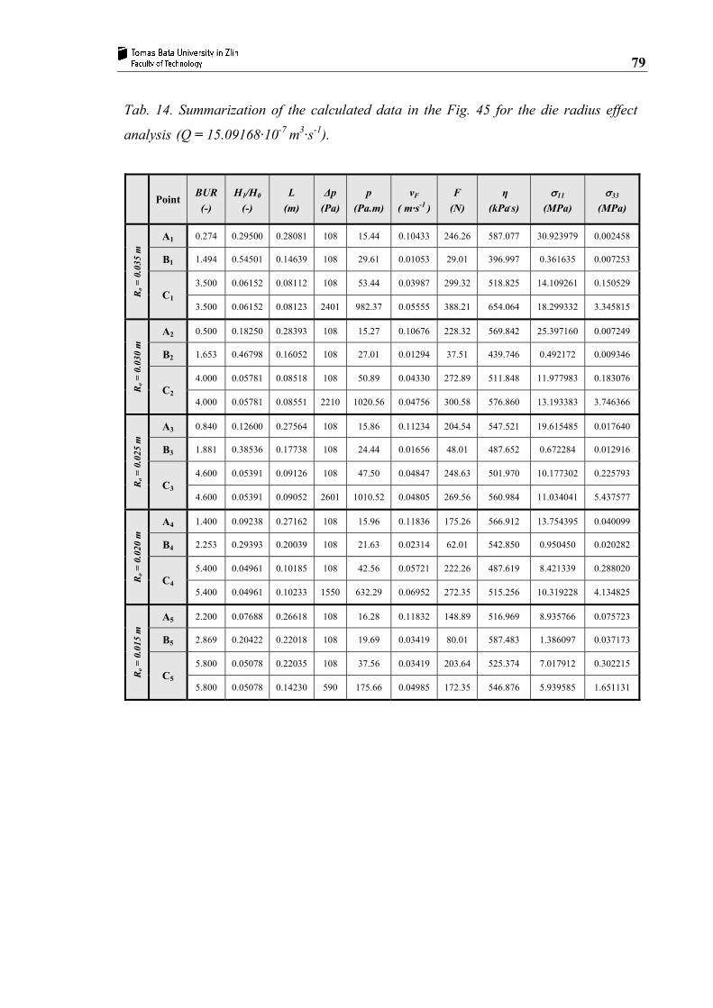
79
Tab. 14. Summarization of the calculated data in the Fig. 45 for the die radius effect
analysis (Q = 15.09168·10-7 m3·s-1).
Point BUR (-)
H1/H0
(-)
L (m)
Δp (Pa)
p (Pa.m)
vF
( m·s-1 ) F
(N) η
(kPa.s) σ11
(MPa) σ33
(MPa)
Ro =
0.0
35 m
A1 0.274 0.29500 0.28081 108 15.44 0.10433 246.26 587.077 30.923979 0.002458
B1 1.494 0.54501 0.14639 108 29.61 0.01053 29.01 396.997 0.361635 0.007253
C1
3.500 0.06152 0.08112 108 53.44 0.03987 299.32 518.825 14.109261 0.150529
3.500 0.06152 0.08123 2401 982.37 0.05555 388.21 654.064 18.299332 3.345815
Ro =
0.0
30 m
A2 0.500 0.18250 0.28393 108 15.27 0.10676 228.32 569.842 25.397160 0.007249
B2 1.653 0.46798 0.16052 108 27.01 0.01294 37.51 439.746 0.492172 0.009346
C2 4.000 0.05781 0.08518 108 50.89 0.04330 272.89 511.848 11.977983 0.183076
4.000 0.05781 0.08551 2210 1020.56 0.04756 300.58 576.860 13.193383 3.746366
Ro =
0.0
25 m
A3 0.840 0.12600 0.27564 108 15.86 0.11234 204.54 547.521 19.615485 0.017640
B3 1.881 0.38536 0.17738 108 24.44 0.01656 48.01 487.652 0.672284 0.012916
C3 4.600 0.05391 0.09126 108 47.50 0.04847 248.63 501.970 10.177302 0.225793
4.600 0.05391 0.09052 2601 1010.52 0.04805 269.56 560.984 11.034041 5.437577
Ro =
0.0
20 m
A4 1.400 0.09238 0.27162 108 15.96 0.11836 175.26 566.912 13.754395 0.040099
B4 2.253 0.29393 0.20039 108 21.63 0.02314 62.01 542.850 0.950450 0.020282
C4 5.400 0.04961 0.10185 108 42.56 0.05721 222.26 487.619 8.421339 0.288020
5.400 0.04961 0.10233 1550 632.29 0.06952 272.35 515.256 10.319228 4.134825
Ro =
0.0
15 m
A5 2.200 0.07688 0.26618 108 16.28 0.11832 148.89 516.969 8.935766 0.075723
B5 2.869 0.20422 0.22018 108 19.69 0.03419 80.01 587.483 1.386097 0.037173
C5 5.800 0.05078 0.22035 108 37.56 0.03419 203.64 525.374 7.017912 0.302215
5.800 0.05078 0.14230 590 175.66 0.04985 172.35 546.876 5.939585 1.651131

80
Tab. 15. Summarization of the calculated data in the Fig. 46 for the mass flow rate
effect analysis.
Point BUR (-)
H1/H0
(-)
L (m)
Δp (Pa)
p (Pa.m)
vF
( m·s-1 ) F
(N) η
(kPa.s) σ11
(MPa) σ33
(MPa)
m =
3.6
kg. h-1
A1 1.400 0.09238 0.27162 108 15.96 0.11836 175.26 566.912 13.754395 0.040099
B1 2.253 0.29393 0.20039 108 21.63 0.02314 62.01 542.850 0.950450 0.020282
C1
5.400 0.04961 0.10185 108 42.56 0.05721 222.26 487.619 8.421339 0.288020
5.400 0.04961 0.10233 1550 632.28 0.09652 272.35 515.256 10.319228 4.133625
m =
5.4
kg. h-1
A2 1.875 0.07930 0.29152 108 19.12 0.13246 187.51 515.739 12.800899 0.062565
B2 2.594 0.23500 0.23322 108 23.90 0.03231 88.01 575.266 1.465441 0.029207
C2 5.900 0.04766 0.12147 108 45.88 0.07003 237.51 480.745 8.574057 0.327585
5.900 0.04766 0.12356 1151 890.56 0.09017 248.65 510.499 8.976209 3.490147
m =
7.2
kg. h-1
A3 2.550 0.06754 0.31479 108 23.61 0.15497 205.63 498.947 12.118612 0.099899
B3 3.093 0.17625 0.27298 108 27.23 0.04812 125.51 594.760 2.336917 0.046434
C3 6.100 0.04675 0.15664 108 55.65 0.09292 275.69 458.965 9.812170 0.345239
6.100 0.04675 0.15594 981 634.56 0.11052 350.21 515.448 12.464435 3.134799
m =
9 k
g. h-1
A4 3.180 0.06100 0.33458 108 27.77 0.15832 219.14 502.611 11.466709 0.137939
B4 3.593 0.13802 0.30408 108 30.55 0.06614 159.51 592.714 3.264823 0.068881
C4 6.400 0.04605 0.18564 108 56.49 0.10585 305.65 495.654 10.526618 0.367739
6.400 0.04605 0.18456 580 298.63 0.12577 310.56 500.156 10.695719 1.975067
m =
10.
8 kg
. h-1 A5 3.800 0.05703 0.34922 108 31.92 0.20123 238.95 468.938 11.191454 0.176304
B5 4.163 0.11500 0.32470 108 34.33 0.08234 185.14 582.274 3.925275 0.095785
C5 6.700 0.45300 0.21546 108 80.56 0.09556 326.48 434.564 1.091837 0.039135
6.700 0.45300 0.21464 331 105.57 0.09856 220.54 561.564 0.737545 0.119779

81
Tab. 16. Summarization of the calculated data in the Fig. 47 for the die /melt
temperature effect analysis (Q = 15.09168·10-7 m3·s-1).
Point BUR (-)
H1/H0
(-)
L (m)
Δp (Pa)
p (Pa.m)
vF
( m·s-1 ) F
(N) η
(kPa.s) σ11
(MPa) σ33
(MPa)
T die =
175
°C
A1 1.400 0.09238 0.27162 108 15.96 0.11836 175.26 566.912 13.754395 0.040099
B1 2.253 0.29393 0.20039 108 21.63 0.02314 62.01 542.850 0.950450 0.020282
C1
5.400 0.04961 0.10185 108 42.56 0.05721 222.26 487.619 8.421339 0.288020
5.400 0.04961 0.10233 1550 632.29 0.06652 272.35 515.256 10.319228 4.133625
T die =
195
°C
A2 1.850 0.06700 0.26937 108 18.79 0.12695 90.52 482.701 7.412626 0.073061
B2 2.568 0.23781 0.21323 108 23.73 0.02544 34.51 559.673 0.573573 0.028573
C2 5.300 0.04370 0.12145 108 42.24 0.06705 111.45 472.365 4.884238 0.320911
5.300 0.04370 0.12254 701 680.53 0.06957 280.46 515.654 12.291014 2.083097
T die =
215
°C
A3 2.230 0.05000 0.23505 108 21.44 0.13739 45.18 492.564 4.112710 0.118007
B3 2.850 0.20035 0.22283 108 25.60 0.02758 19.89 571.048 0.353566 0.037639
C3 5.200 0.03984 0.13837 108 41.23 0.07604 58.68 460.106 2.874736 0.345327
5.200 0.03984 0.13646 651 690.56 0.07806 295.66 555.631 14.484395 2.080146
T die =
235
°C
A4 2.550 0.04605 0.27323 108 23.11 0.13045 25.12 552.628 2.171320 0.146521
B4 3.050 0.17154 0.23336 108 26.93 0.03055 12.79 582.020 0.248136 0.047047
C4 4.950 0.03816 0.16051 108 41.57 0.08106 35.56 450.105 1.910631 0.343195
4.950 0.03816 0.16245 426 125.99 0.08212 150.64 525.325 8.093853 1.352602
T die =
255
°C
A5 2.865 0.04100 0.27092 108 25.14 0.13041 13.87 564.261 1.198511 0.184897
B5 3.231 0.14901 0.24211 108 28.15 0.03364 8.64 589.516 0.182153 0.057374
C5 4.640 0.03598 0.15154 108 44.95 0.09175 20.67 447.544 1.256571 0.341192
4.640 0.03598 0.16546 261 98.54 0.08505 19.85 550.681 1.206722 0.822967

82
Tab. 17. Summarization of the calculated data in the Fig. 48 for the cooling air
temperature effect analysis (Q = 15.09168·10-7 m3·s-1).
Point BUR (-)
H1/H0
(-)
L (m)
Δp (Pa)
p (Pa.m)
vF
( m·s-1 ) F
(N) η
(kPa.s) σ11
(MPa) σ33
(MPa)
T air =
10
°C
A1 1.100 0.12156 0.27043 108 13.97 0.11456 178.89 545.077 13.578945 0.023943
B1 1.994 0.35240 0.18969 108 19.91 0.02182 53.01 522.537 0.765730 0.014972
C1
5.000 0.05703 0.09465 108 39.90 0.05371 231.26 493.280 8.231777 0.231979
5.000 0.05703 0.09564 1651 480.65 0.05951 280.56 523.560 9.986627 3.545414
T air =
25
°C
A2 1.400 0.09238 0.27162 108 15.96 0.11836 175.26 566.912 13.754395 0.040099
B2 2.253 0.29393 0.20039 108 21.63 0.02314 62.01 542.850 0.950450 0.020282
C2 5.400 0.04961 0.10185 108 42.56 0.05721 222.26 487.619 8.421339 0.288020
5.400 0.04961 0.10233 1550 632.28 0.07652 272.35 515.256 10.319228 4.133625
T air =
40
°C
A3 1.850 0.06853 0.26545 108 19.52 0.11259 172.56 509.632 13.815144 0.071429
B3 2.594 0.23432 0.21340 108 23.90 0.02519 74.51 564.407 1.244239 0.029292
C3 5.900 0.04219 0.11114 108 45.88 0.06154 212.51 481.278 8.665877 0.370044
5.900 0.04219 0.11235 1290 458.96 0.04953 198.45 512.354 8.092528 4.418698
T air =
55
°C
A4 2.512 0.05055 0.25464 108 23.56 0.12565 170.56 478.062 13.634137 0.131494
B4 3.153 0.17525 0.22536 108 27.62 0.02772 88.51 583.048 1.625865 0.047605
C4 6.600 0.03458 0.12154 108 50.46 0.07055 203.54 470.812 9.052740 0.505049
6.600 0.03458 0.12589 854 367.65 0.05966 275.65 525.459 12.259938 3.995783
T air =
70
°C
A5 3.640 0.03271 0.26054 108 30.90 0.12868 170.5 497.883 14.537272 0.294494
B5 4.093 0.11701 0.23883 108 33.88 0.03197 107.51 595.224 2.278646 0.092561
C5 7.200 0.02500 0.15546 108 55.23 0.08510 198.53 459.564 11.194645 0.762018
7.200 0.02500 0.14567 497 238.24 0.05642 212.56 545.489 11.985764 3.503587
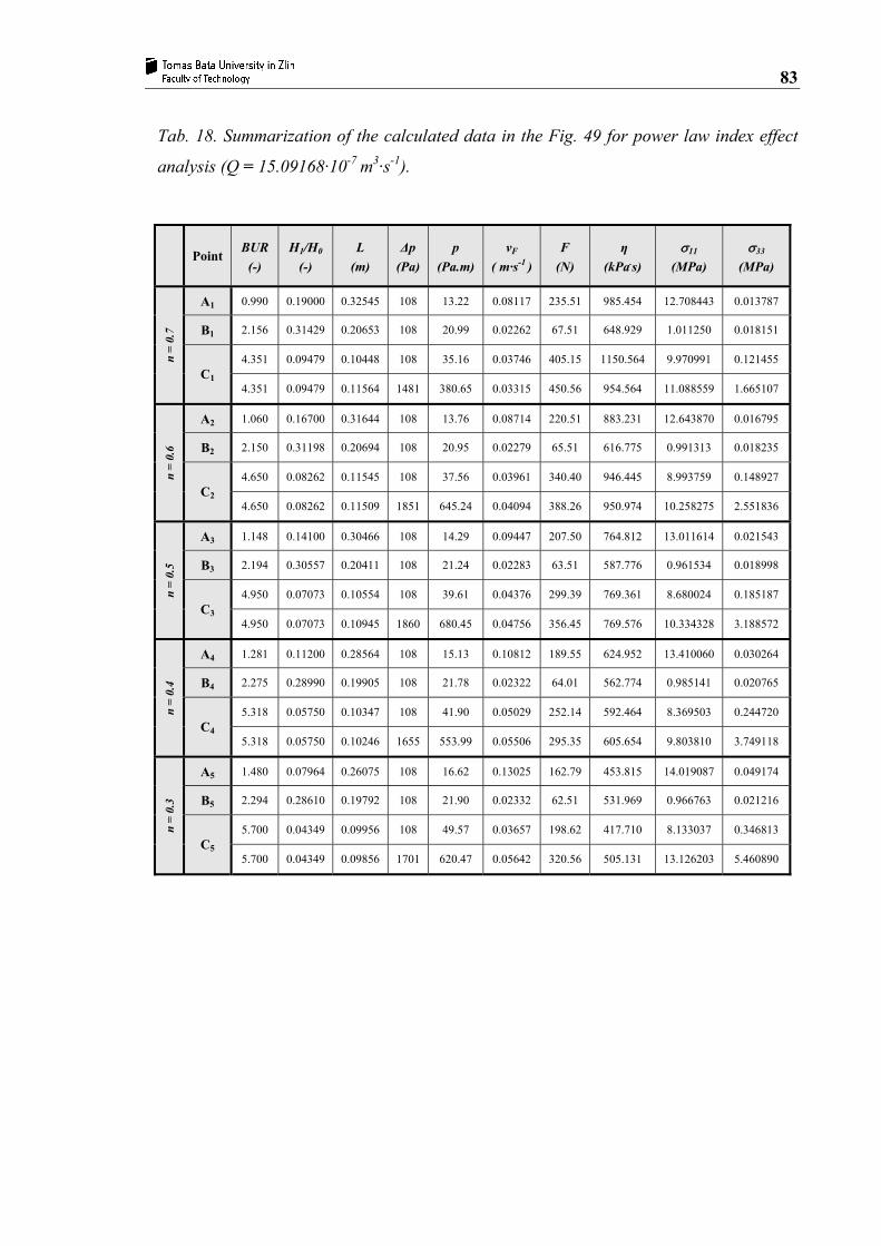
83
Tab. 18. Summarization of the calculated data in the Fig. 49 for power law index effect
analysis (Q = 15.09168·10-7 m3·s-1).
Point BUR (-)
H1/H0
(-)
L (m)
Δp (Pa)
p (Pa.m)
vF
( m·s-1 ) F
(N) η
(kPa.s) σ11
(MPa) σ33
(MPa)
n =
0.7
A1 0.990 0.19000 0.32545 108 13.22 0.08117 235.51 985.454 12.708443 0.013787
B1 2.156 0.31429 0.20653 108 20.99 0.02262 67.51 648.929 1.011250 0.018151
C1
4.351 0.09479 0.10448 108 35.16 0.03746 405.15 1150.564 9.970991 0.121455
4.351 0.09479 0.11564 1481 380.65 0.03315 450.56 954.564 11.088559 1.665107
n =
0.6
A2 1.060 0.16700 0.31644 108 13.76 0.08714 220.51 883.231 12.643870 0.016795
B2 2.150 0.31198 0.20694 108 20.95 0.02279 65.51 616.775 0.991313 0.018235
C2 4.650 0.08262 0.11545 108 37.56 0.03961 340.40 946.445 8.993759 0.148927
4.650 0.08262 0.11509 1851 645.24 0.04094 388.26 950.974 10.258275 2.551836
n =
0.5
A3 1.148 0.14100 0.30466 108 14.29 0.09447 207.50 764.812 13.011614 0.021543
B3 2.194 0.30557 0.20411 108 21.24 0.02283 63.51 587.776 0.961534 0.018998
C3 4.950 0.07073 0.10554 108 39.61 0.04376 299.39 769.361 8.680024 0.185187
4.950 0.07073 0.10945 1860 680.45 0.04756 356.45 769.576 10.334328 3.188572
n =
0.4
A4 1.281 0.11200 0.28564 108 15.13 0.10812 189.55 624.952 13.410060 0.030264
B4 2.275 0.28990 0.19905 108 21.78 0.02322 64.01 562.774 0.985141 0.020765
C4 5.318 0.05750 0.10347 108 41.90 0.05029 252.14 592.464 8.369503 0.244720
5.318 0.05750 0.10246 1655 553.99 0.05506 295.35 605.654 9.803810 3.749118
n =
0.3
A5 1.480 0.07964 0.26075 108 16.62 0.13025 162.79 453.815 14.019087 0.049174
B5 2.294 0.28610 0.19792 108 21.90 0.02332 62.51 531.969 0.966763 0.021216
C5 5.700 0.04349 0.09956 108 49.57 0.03657 198.62 417.710 8.133037 0.346813
5.700 0.04349 0.09856 1701 620.47 0.05642 320.56 505.131 13.126203 5.460890

84
Tab. 19. Summarization of the calculated data in the Fig. 50 for the flow activation
effect analysis (Q = 15.09168·10-7 m3·s-1).
Point BUR (-)
H1/H0
(-)
L (m)
Δp (Pa)
p (Pa.m)
vF
( m·s-1 ) F
(N) η
(kPa.s) σ11
(MPa) σ33
(MPa)
EA =
75
kJ. m
ol -1
A1 1.410 0.08900 0.27162 108 15.96 0.12180 208.76 509.964 16.885435 0.041920
B1 2.269 0.29110 0.19943 108 21.73 0.02320 66.01 540.202 1.014395 0.020624
C1
5.600 0.04843 0.09877 108 43.88 0.05648 252.26 481.130 9.441043 0.305959
5.600 0.04843 0.10054 1225 582.32 0.04532 286.54 512.235 10.724001 3.470370
EA =
60
kJ. m
ol -1
A2 1.382 0.09316 0.27162 108 15.96 0.11620 154.82 538.060 12.205726 0.039253
B2 2.289 0.28685 0.19819 108 21.87 0.02331 61.51 549.172 0.950866 0.021114
C2 5.400 0.05039 0.10186 108 42.56 0.05627 201.14 495.848 7.502991 0.283556
5.400 0.05039 0.10345 1450 523.56 0.04694 228.45 512.566 8.521717 3.807005
EA =
45
kJ. m
ol -1
A3 1.347 0.09936 0.27564 108 15.75 0.12066 110.56 563.463 8.384804 0.035871
B3 2.241 0.29505 0.20116 108 21.55 0.02319 48.89 547.028 0.750510 0.020097
C3 5.100 0.05310 0.10686 108 40.56 0.05655 155.19 520.022 5.816652 0.254136
5.100 0.05310 0.10584 1520 562.54 0.00534 192.15 532.045 7.201944 3.576723
EA =
30
kJ. m
ol -1
A4 1.332 0.10300 0.28343 108 15.29 0.11253 72.32 583.941 5.350459 0.034218
B4 2.253 0.29203 0.20038 108 21.63 0.02327 33.32 535.878 0.514032 0.020414
C4 4.700 0.05703 0.11436 108 37.90 0.05712 114.89 547.310 4.350659 0.218064
4.700 0.05703 0.11354 1220 418.56 0.04846 131.56 565.256 4.981920 2.463318
EA =
15
kJ. m
ol -1
A5 1.325 0.10500 0.28343 108 15.29 0.11090 45.51 593.072 3.320288 0.033390
B5 2.281 0.28622 0.19897 108 21.82 0.02345 21.66 522.162 0.336750 0.021087
C5 4.544 0.60004 0.11853 108 36.57 0.05699 80.45 570.733 0.299489 0.020038
4.544 0.60004 0.11759 1220 416.47 0.05522 98.29 579.312 0.365902 0.226352

85
Tab. 20. Zatloukal-Vlcek film blowing model parameters including Newtonian viscosity,
η0, for generalized Newtonian constitutive equation.
η0 (kPa·s)
L (m)
Q
( m3·s-1 ) p
( Pa·m )σ
(MPa) H0 (m)
R0 (m)
Fig. 57-58 100 0.18 43.40·10-7 50 0.3 1.9 2.5
1.34·10-3 0.037
Fig. 53-56 100 0.18 43.40·10-7 111.163 1 1.34·10-3 0.037
Fig. 51-52 2449103 244910.3 24491.03
0.18 43.40·10-7 111.163 1 1.34·10-3 0.037
Tab. 21. Parameters of the generalized Newtonian constitutive equation.
β (-)
λ (s)
ξ (-)
a (-)
n (-)
α (s)
Fig. 57-58 1 0.23591 0.565997 0.76966 0.28329 0
0.2 1
Fig. 53-54 1 0.23591
0.0 0.2 0.4 0.6 0.8
0.76966 0.28329 0.5
Fig. 55-56 1 0.23591 0.565997 0.76966 0.28329
0 0.1 0.5
1 1.5
Fig. 51-52 1 77.4 2.58 0.086
0 0.41 0.28329 0

86
10-4 10-3 10-2 10-1 100 101 102 103 104
Extensional and shear rates ε, γ (1/s)
101
102
103
104
105
106
She
ar a
nd e
xten
sion
al v
isco
sitie
s η,
ηΕ (
Pa. s
)
LDPE shear and uniaxial extensional viscositiesGeneralized Newtonian model fit
Fig. 36. Comparison between generalized Newtonian model fitting lines and experimental
data for LDPE material taken from Tas's Ph.D. thesis [1].

87
0 0.02 0.04 0.06 0.08 0.1 0.12 0.14 0.16 0.18 0.2 0.22
x (m)
0.016
0.02
0.024
0.028
0.032
0.036
0.04
y (m
)
Experimental dataZatloukal-Vlcek model prediction
Fig. 37. Comparison between Zatloukal-Vlcek model predictions and experimental data for
the LDPE bubble shape taken from Tas's Ph.D. thesis [1].

88
0 0.02 0.04 0.06 0.08 0.1 0.12 0.14 0.16 0.18 0.2 0.22
x (m)
0
0.02
0.04
0.06
0.08
0.1
v (m
)
Experimental dataNon-isothermal Zatloukal-Vlcek modelIsothermal Zatloukal-Vlcek modelImproved non-isothermal Zatloukal-Vlcek model
F = 17.36 NF = 3.16 N
F = 14.61 N
Fig. 38. Comparison between non-Newtonian Zatloukal-Vlcek model predictions and
experimental data for the LDPE bubble velocity taken from Tas's Ph.D. thesis [1].

89
0 0.02 0.04 0.06 0.08 0.1 0.12 0.14 0.16 0.18 0.2 0.22
x (m)
70
80
90
100
110
120
130
140
150
160
170
180
T (°
C)
Experimental dataNon-isothermal Zatloukal-Vlcek modelImproved non-isothermal Zatloukal-Vlcek model
Fig. 39. Comparison between non-Newtonian Zatloukal-Vlcek model predictions and
experimental data for the LDPE bubble temperature taken from Tas's Ph.D. thesis [1].

90
0 2 4 6
BUR
0
0.1
0.2
0.3
0.4
H1 / H
0
UNSTABLESTABLE
Model stability contour
Model stability contour for different internal bubble pressure Δp values
Machine stability contourCircumferential stability contour
Fig. 40. Typical processing window predicted by the Zatloukal-Vlcek model for
non-isothermal processing conditions and non-Newtonian polymer melt.

91
0 1 2 3 4 5 6
BUR
0
0.1
0.2
0.3
0.4
0.5
H1 /
H0
η0 = 50 kPa.s
η0 = 100 kPa.s
η0 = 200 kPa.s
η0 = 300 kPa.s
η0 = 400 kPa.s
A1
B1
C1
A2
B2
C2A3
B3
C3,4,5
A4
B4
A5
B5
UNSTABLE
STABLE
Fig. 41. Stability contours for different level of the Newtonian viscosity predicted by the
Zatloukal-Vlcek model for non-isothermal processing conditions and non-Newtonian
polymer melt. Model and machine stability contours are represented by triangles and
circles, respectively.

92
0 2 4 6 8
BUR
0
0.1
0.2
0.3
0.4
0.5
H1 /
H0
h = 30 W.m-2.K-1
h = 40 W.m-2.K-1
h = 50 W.m-2.K-1
h = 60 W.m-2.K-1
h = 70 W.m-2.K-1
A1
B1
C1
A2
B2
C2
A3
B3
C3
A4
B4
C4A5
B5
C5
UNSTABLE
STABLE
Fig. 42. Stability contours for different level of the heat transfer coefficient predicted by
the Zatloukal-Vlcek model for non-isothermal processing conditions and non-Newtonian
polymer melt. Model and machine stability contours are represented by triangles and
circles, respectively.

93
0 1 2 3 4 5 6
BUR
0
0.1
0.2
0.3
0.4
0.5
H1 /
H0
Δp = 50 PaΔp = 100 PaΔp = 200 PaΔp = 300 PaΔp = 400 PaΔp = 500 PaΔp = 700 Pa
A1
B1
A2
B2
A3
B3
A4
B4
A5
B5
UNSTABLE
STABLE
B6
A6 D6
C6
B7
A7
C7
C1,2,3,4,5
Fig. 43. Stability contours for different level of the internal bubble pressure predicted by
the Zatloukal-Vlcek model for non-isothermal processing conditions and non-Newtonian
polymer melt. Model, machine and circumference stability contours are represented by
triangles, circles and squares, respectively.

94
0 2 4 6
BUR
0
0.1
0.2
0.3
0.4
H1 /
H0
σ = 0.15 MPaσ = 0.20 MPaσ = 0.40 MPaσ = 0.60 MPaσ = 0.80 MPaσ = 1.00 MPa
A1
B1,2,3,4,5,6
C1
A3
C3
A4
C4
A5
C5
A6
C6
UNSTABLE
STABLE
A2
C2
Fig. 44. Stability contours for different level of the rupture stress predicted by the
Zatloukal-Vlcek model for non-isothermal processing conditions and non-Newtonian
polymer melt. Model and machine stability contours are represented by triangles and
circles, respectively.

95
0 2 4 6
BUR
0
0.2
0.4
0.6
0.8
H1 /
H0
R0 = 0.015 mR0 = 0.020 mR0 = 0.025 mR0 = 0.030 mR0 = 0.035 m
A1
B1
C1
A2
B2
C2
A3
B3
C3
A4
B4
C4
A5
B5
C5
UNSTABLE
STABLE
Fig. 45. Stability contours for different level of the die radius predicted by the
Zatloukal-Vlcek model for non-isothermal processing conditions and non-Newtonian
polymer melt. Model and machine stability contours are represented by triangles and
circles, respectively.

96
0 2 4 6 8
BUR
0
0.1
0.2
0.3
0.4
H1 /
H0
m = 3.6 kg.h-1
m = 5.4 kg.h-1
m = 7.2 kg.h-1
m = 9.0 kg.h-1
m = 10.8 kg.h-1
A1
B1
C1
A2
B2
C2
A3
B3
C3
A4
B4
C4A5
B5
C5
UNSTABLE
STABLE
Fig. 46. Stability contours for different level of the mass flow rate predicted by the
Zatloukal-Vlcek model for non-isothermal processing conditions and non-Newtonian
polymer melt. Model and machine stability contours are represented by triangles and
circles, respectively.

97
0 2 4 6
BUR
0
0.1
0.2
0.3
0.4
H1 /
H0
Tdie = 255 °CTdie = 235 °CTdie = 215 °CTdie = 195 °CTdie = 175 °C
A1
B1
C1A2
B2
C2A3
B3
C3A4
B4
C4A5
B5
C5
UNSTABLE
STABLE
Fig. 47. Stability contours for different level of the melt/die temperature predicted by the
Zatloukal-Vlcek model for non-isothermal processing conditions and non-Newtonian
polymer melt. Model and machine stability contours are represented by triangles and
circles, respectively.
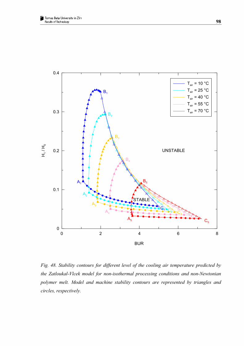
98
0 2 4 6 8
BUR
0
0.1
0.2
0.3
0.4
H1 /
H0
Tair = 10 °CTair = 25 °CTair = 40 °CTair = 55 °CTair = 70 °C
A1
B1
C1
A2
B2
C2
A3
B3
C3A4
B4
C4A5
B5
C5
UNSTABLE
STABLE
Fig. 48. Stability contours for different level of the cooling air temperature predicted by
the Zatloukal-Vlcek model for non-isothermal processing conditions and non-Newtonian
polymer melt. Model and machine stability contours are represented by triangles and
circles, respectively.
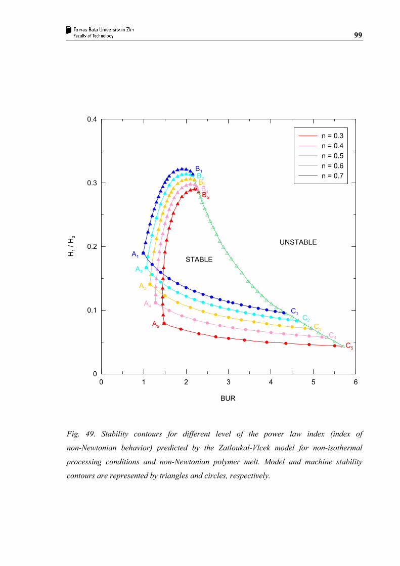
99
0 1 2 3 4 5 6
BUR
0
0.1
0.2
0.3
0.4
H1 /
H0
n = 0.3n = 0.4n = 0.5n = 0.6n = 0.7
A1
B1
C1
A2
B2
C2
A3
B3
C3
A4
B4
C4
A5
B5
C5
UNSTABLE
STABLE
Fig. 49. Stability contours for different level of the power law index (index of
non-Newtonian behavior) predicted by the Zatloukal-Vlcek model for non-isothermal
processing conditions and non-Newtonian polymer melt. Model and machine stability
contours are represented by triangles and circles, respectively.

100
0 2 4 6
BUR
0
0.1
0.2
0.3
0.05
0.15
0.25
0.35
H1 /
H0
Ea = 15 kJ.mol-1
Ea = 30 kJ.mol-1
Ea = 45 kJ.mol-1
Ea = 60 kJ.mol-1
Ea = 75 kJ.mol-1
A1
B1
C1
A2
B2
C2
A3
B3
C3
A4
B4
C4
A5
B5
C5
UNSTABLE
STABLE
Fig. 50. Stability contours for different level of the flow activation energy predicted by the
Zatloukal-Vlcek model for non-isothermal processing conditions and non-Newtonian
polymer melt. Model and machine stability contours are represented by triangles and
circles, respectively.

101
10-5 10-4 10-3 10-2 10-1 100 101 102 103 104
Shear rate γ (1/s)
102
103
104
105
106
107
She
ar v
isco
sity
η (P
a.s)
η0 = 2449103 Pa.s, λ = 77.4 s
η0 = 244910.3 Pa.s, λ = 2.58 s
η0 = 24491.03 Pa.s, λ = 0.086 s
Fig. 51. Shear viscosity prediction of the generalized Newtonian model for different values
of η0 and λ (effect of Mw).

102
0 10 20 30 40 50
BUR
0
0.01
0.02
0.03
0.04
0.05
0.06
0.07
0.08
0.09
H1 / H
0
η = 2 449 103 Pa.s, λ = 77.4 sη = 244 910.3 Pa.s, λ = 2.58 sη = 24 491.03 Pa.s, λ = 0.086 s
STABLE
UNSTABLE
Fig. 52. Predicted film blowing stability contours for three virtual materials (Fig. 51) by
using Zatloukal-Vlcek film blowing model (effect of Mw). Processing conditions are
provided in Tab. 20.

103
10-3 10-2 10-1 100 101 102 103 104
Extensional and shear rates ε, γ (1/s)
102
103
104
105
106
107
shea
r and
ext
ensi
onal
vis
cosi
ties
η, η
Ε (P
a. s)
Extensional viscosity, ξ = 0Extensional viscosity, ξ = 0.2Extensional viscosity, ξ = 0.4Extensional viscosity, ξ = 0.6Extensional viscosity, ξ = 0.8Shear viscosity
Fig. 53. Shear and extensional viscosity prediction of the generalized Newtonian model for
different values of ξ (different level long chain branching).

104
0 2 4 6 8 10
BUR
0
0.01
0.02
0.03
0.04
0.05
0.06
0.07
0.08
0.09
H1 /
H0
ξ = 0ξ = 0.2ξ = 0.4ξ = 0.6ξ = 0.8
STABLE
UNSTABLE
111.56
124.89
Fig. 54. Predicted film blowing stability contours for five virtual materials (Fig. 53) by
using Zatloukal-Vlcek film blowing model (effect of long chain branching). Processing
conditions are provided in Tab. 20.

105
10-3 10-2 10-1 100 101 102 103 104
Extensional and shear rates ε, γ (1/s)
102
103
104
105
106
107
Shea
r and
ext
ensi
onal
vis
cosi
ties
η, η
Ε (P
a. s)
Extensional viscosity, α = 0 sExtensional viscosity, α = 0.1 sExtensional viscosity, α = 0.5 sExtensional viscosity, α = 1.0 sExtensional viscosity, α = 1.5 sShear viscosity
Fig. 55. Shear and extensional viscosity prediction of the generalized Newtonian model for
different values of α (different level long chain branching).

106
0 1 2 3 4 5 6 7 8 9 10
BUR
0.01
0.015
0.02
0.025
0.03
H1 /
H0
α = 0 sα = 0.1 sα = 0.5 sα = 1.0 sα = 1.5 s
UNSTABLE
STABLE
Fig. 56. Predicted film blowing stability contours for five virtual materials (Fig. 55) by
using Zatloukal-Vlcek film blowing model (effect of long chain branching). Processing
conditions are provided in Tab. 20.
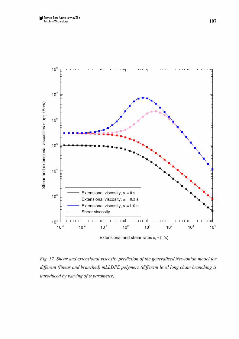
107
10-3 10-2 10-1 100 101 102 103 104
Extensional and shear rates ε, γ (1/s)
102
103
104
105
106
107
108
She
ar a
nd e
xten
sion
al v
isco
sitie
s η,
ηΕ
(P
a.s)
Extensional viscosity, α = 0 sExtensional viscosity, α = 0.2 sExtensional viscosity, α = 1.0 sShear viscosity
Fig. 57. Shear and extensional viscosity prediction of the generalized Newtonian model for
different (linear and branched) mLLDPE polymers (different level long chain branching is
introduced by varying of α parameter).

108
1 1.2 1.4 1.6 1.8 2 2.2 2.4 2.6 2.8 3 3.2
BUR
0
0.005
0.01
0.015
0.02
0.025
0.03
0.035
0.04
0.045
0.05
0.055
0.06
H1 /
H0
σ33 = 0.3 MPa
σ33 = 1.9 MPa
σ33 = 2.5 MPaLinear mLLDPEHigh mLLDPEMiddle mLLDPE
STABLE
UNSTABLE
Fig. 58. Comparison between experimental data taken from [54] and predicted film
blowing stability contours (lines) for linear and branched mLLDPE polymers (Fig. 57) by
using Zatloukal-Vlcek film blowing model. Model parameters are provided in Tabs. 20-21.

109
BIBLIOGRAPHY
[1] TAS, P.P. Film blowing from polymer to product. Ph.D. Thesis, Technische
Universitat Eindhoven, 1994.
[2] KOLARIK, R. Modeling of the film blowing process by using variational
principles. Bc. Thesis, Tomas Bata University in Zlín, Czech Republic, 2006.
[3] CANTOR, K. Blown Film Extrusion. Munich : Cark Hanser Verlag, 2006. 165 s.
ISBN 1-56990-396-4.
[4] LUO, X. L., TANNER, R. I. A computer study of film blowing. Polym. Eng. Sci.
25, p. 620, 1985.
[5] ASHOK, B. K., CAMPBELL, G. A. Two-phase simulation of tubular film
blowing of crystalline polymers. Int. Polym. Process. 7, 240, 1992.
[6] ZATLOUKAL, M., VLCEK, J. Application of variational principles in modeling
of the film blowing process for high stalk bubbles. J. Non-Newtonian Fluid Mech.
133, p. 63-72, 2006.
[7] ZATLOUKAL, M., VLCEK, J. Modeling of the film blowing process by using
variational principles. J. Non-Newtonian Fluid Mech. 123, p. 201-213, 2004.
[8] ZATLOUKAL, M., MAVRIDIS, H., VLCEK, J., SAHA, P. Modeling of
Non-isothermal Film Blowing Process by Using Variational Principles. SPE
ANTEC, p. 825-829, Charlotte, USA, 2006.
[9] ZATLOUKAL, M., SAHA, P. Modeling of the film blowing process by using
variational principles for high stalk bubbles. PPS-21, Leipzig, Germany, 2005
(CD-ROM).
[10] KANAI, T., CAMPBELL, G. A. Film Processing: Progress in Polymer
Processing. Hanser Gardner Publications, Munich, Germany, 1999.
[11] MAYAVARAM, R. S. Modeling and simulation of film blowing process. Ph.D.
Thesis, A&M University Texas, 2005.
[12] HAN, Ch. D. Rheology in Polymer Processing. New York : Academic Press,
1976. 366 s. ISBN 0-12-322450-0.
[13] BUTLER, T. I. Film extrusion Manual : Process, materials, properties. Atlanta :
Tappi press, 2005. 616 s. ISBN 1-59510-075-X.

110
[14] HAN, Ch. D. Rheology and Processing of Polymeric Materials : Volume 2
Polymer Processing. New York : Oxford University Press, 2007. 579 s.
ISBN 978-0-19-518783-0.
[15] BAIRD, D. G., COLLIAS, D. I. Polymer Processing : Principles and Design.
Canada : John Wiley & Sons, 1998. 346 s. ISBN 0-471-25453-3.
[16] PEARSON, J. R., PETRIE, C. J. S. The flow of a tubular film. Part 2. Interpreta-
tion of the model and discussion of solutions. J. Fluid Mech. 42, p. 60, 1970.
[17] AGASSANT, J. F., AVENAS, P., SERGENT, J. Ph., CARREAU, P. J. Polymer
processing: Principles and modeling, Carl Hanser, Munich, Gremany, 1991.
[18] BUTLER, T. I. Blown film bubble instability induced by fabrication conditions.
SPE ANTEC Tech. Papers 1, p. 1120, 2000.
[19] HAN, C. D., PARK, J. Y. Studies on blown film extrusion: Part 3. Bubble
instability. J. Appl. Polymer Sci. 19, p. 3291, 1975.
[20] HAN, C. D., SHETTY, R. Flow instability in tubular film blowing: Part 1.
Experimental study. Ind. Eng. Chem. Fund., 16, p. 49, 1977.
[21] OBIJESKI, T. J., PURITT, K. R. Improving the output and bubble stability of
thick gauge blown film. SPE ANTEC Tech. Papers 1, p. 150, 1992.
[22] KANAI, T., WHITE, J. L. Kinematics, dynamics and stability of the tubular film
extrusion of various polyethylenes. J. Non-Newtonian Fluid Mech. 19, p. 275,
1986.
[23] SWEENEY, P. A., CAMPBELL, G. A. Blown film stability. ANTEC 461, p. 461,
1993.
[24] LAFUENTE-CANAS, P., FERNÁNDEZ AMO, B., SMITH, G. D., SPARES, R.,
MARTYN, M. T., COATES, P. D. Blown Film: processing stability for metallo-
cenes. in: Polymer Process Engineering 03: Enhanced Polymer Processing, p.
192-213. Edited by PD Coates, University Press, Bradford, UK, 2003.
[25] WALLER, P. What to do when the bubble won´t behave. Plastic Technology,
(December 2002), p.36
[26] ZATLOUKAL, M. Differential viscoelastic constitutive equations for polymer
melts in steady shear and elongational flows. J. Non-Newtonian Fluid Mech. 113,
209, 2003.

111
[27] KIM, S., FANG, Y., LAFLEUR, P. G., CARREAU, P. J. Dynamics and criteria
for bubble instabilities in a single layer film blowing extrusion. Polymer
Engineering and Science, 4, 2, 2004.
[28] DEBBAUT, B. et. al. Intern. Polym. Process., 13, 3, p. 262, 1999.
[29] WANG, S.Q. Advances in Polymer Science, 138, p. 229, 1999.
[30] SIDIROPOULOS, V., VLACHOPOULOS, J. Numerical study of internal bubble
cooling (IBC) in film blowing. Polymer Processing, 16, 1, 2001.
[31] SIDIROPOULOS, V., VLACHOPOULOS, J. An investigation of Venturi and
Coanda effects in blown film cooling. Polymer Processing, 15, 1, 2000.
[32] ZHANG, Z., LAFLEUR, P. G., BERTRAND, F. Effect of aerodynamics on film
blowing process. Polymer Processing, 21, 5, 2006.
[33] SIDIROPOULOS, V., VLACHOPOULOS, J. The aerodynamics of blown film
bubble cooling. Journal of Reinforced Plastics and Composites, 18, 6, p. 529-538,
1999.
[34] MUKE, S., CONNELL, H., SBARSKI, I., BHATTACHARYA, S. N. Numerical
modeling and experimental verification of blown film processing. J. Non-
Newtonian Fluid Mech. 116, p. 113-138, 2003.
[35] PEARSON, J. R. A., PETRIE, C. J. S. The flow of a tubular film. Part 1. Formal
mathematical representation. J. Fluid Mech. 40, p. 1, 1970.
[36] PETRIE, C. J. S. A comparison of theoretical predictions with published
experimental measurements on the blown film process. Am. Inst. Chem. Eng. J.
21, p. 275, 1975.
[37] HAN, C. D., PARK, J. Y. Studies on blown film extrusion. 2. Analysis of the de-
formation and heat transfer process. J. Appl. Polym. Sci. 19, p. 3277-3290, 1975.
[38] WAGNER, M. H. Das folienblasverfahren als rheologish-thermodynamischer
PozeB. Rheol. Acta 15, p. 40-51, 1976.
[39] PEARSON, J. R., GUTTERIDGE, P. A. Stretching flow for thin film production.
Part 1. Bubble blowing in the solid phase. J. Non-Newtonian Fluid Mech. 4,
p. 57-72, 1978.
[40] GUPTA, R. K., METZNER, A. B., WISSBRUN, K. F. Modeling of polymeric
film-blowing processes. Polym. Eng. Sci. 22, 172, 1982.
112
[41] KANAI, T., WHITE, J. L. Dynamics, heat transfer and structure development in
tubular film extrusion of polymer melts: a mathematical model and predictions. J.
Polym. Eng. 5, p. 135, 1985.
[42] CAIN, J. J., DENN, M. M. Multiplicities and instabilities in film blowing. Polym.
Eng. Sci. 28, p. 1527, 1988.
[43] SEO, Y., WISSLER, E. H. The effect of extrude swell on modeling the film
blowing process. Polym. Eng. Sci. 29, 722, 1989.
[44] CAMPBELL, G. A., CAO, B. Blown film simulation, A severe test for rheological
models. in: Collyer, A.A.a.U.L.A. (Ed.), Polymer Rheology and Processing,
Elsevier, Amsterdam, 1990.
[45] CAO, B., CAMPBELL, G. A. Viscoplastic-elastic modeling of tubular blown film
processing. Am. Inst. Chem. Eng. J. 36, p. 420, 1990.
[46] ALAIE, S. M., PAPANASTASIOU, T. C. Modeling of non-isothermal film
blowing with integral constitutive equations. Int. Polym. Process. 8, p. 51-65,
1993.
[47] LIU, C. C., BOQUE, D. C., SPRUIELL J. E. Tubular film blowing. Part 2.
Theoretical modeling. Int. Polym. Process. 10, p. 230, 1995.
[48] SIDIROPOULOS, V., VLACHOPOULOS, J. Computer simulation of film
blowing. in: Proceeding of the ANTEC, p. 31-39, 1996.
[49] SIDIROPOULOS, V., TIAN, J. J., VLACHOPOULOS, J. Computer simulation of
film blowing. TAPPI J. 79, p. 113-118, 1996.
[50] KUIJK, E. W., TAS, P. P., NEUTEBOOM, P. A rheological model for the
prediction of polyethylene blown film properties. SPE ANTEC 98, 3001, 1998.
[51] SPENCER, R. S., GILMORE, R. D. J. Appl. Phys., p. 21-523, 1950.
[52] HELLWEGE, K. H., KNAPPE, W., LEHMANN, P., KOLLOID, Z. Polymere.
183, p. 110-120, 1962.
[53] Xpansion Intruments, www.xinst.com [online]. c2005 [cit. 2008-05-22]. Available
at WWW: <http://www.xinst.com/products_modes.htm>.
[54] ZATLOUKAL, M., KOLARIK, R., MUSIL, J., MARTYN, M., COATES, P.
Investigation of film blowing process stability for metallocene based LLDPE with
different level of long chain branching. SPE ANTEC, p. 1573-1578, 2007.

113
[55] DOUFAS, A. K., McHUGH, A. J. Simulation of film blowing including
flow-induced crystallization. J. Rheology. 45 (5), 1085, 2001.
[56] ZATLOUKAL, M., MAVRIDIS, H., VLCEK, J., SAHA, P. Modeling of
Non-Isothermal high stalk film blowing process by using variational principles for
Non-Newtonian fluids. SPE ANTEC, p. 1579-1583, 2007.
[57] MUSIL, J. The effect of long chain branching on processibility of polymer melts.
Bc. Thesis, Tomas Bata University in Zlín, Czech Republic, 2006.
[58] MUNSTEDT, H., STEFFL, T., MALMBERG, A. Correlation between
rheological behaviour in uniaxial elongation and film blowing properties of
various polyethylenes. Rheol Acta 45, 14, 2005.
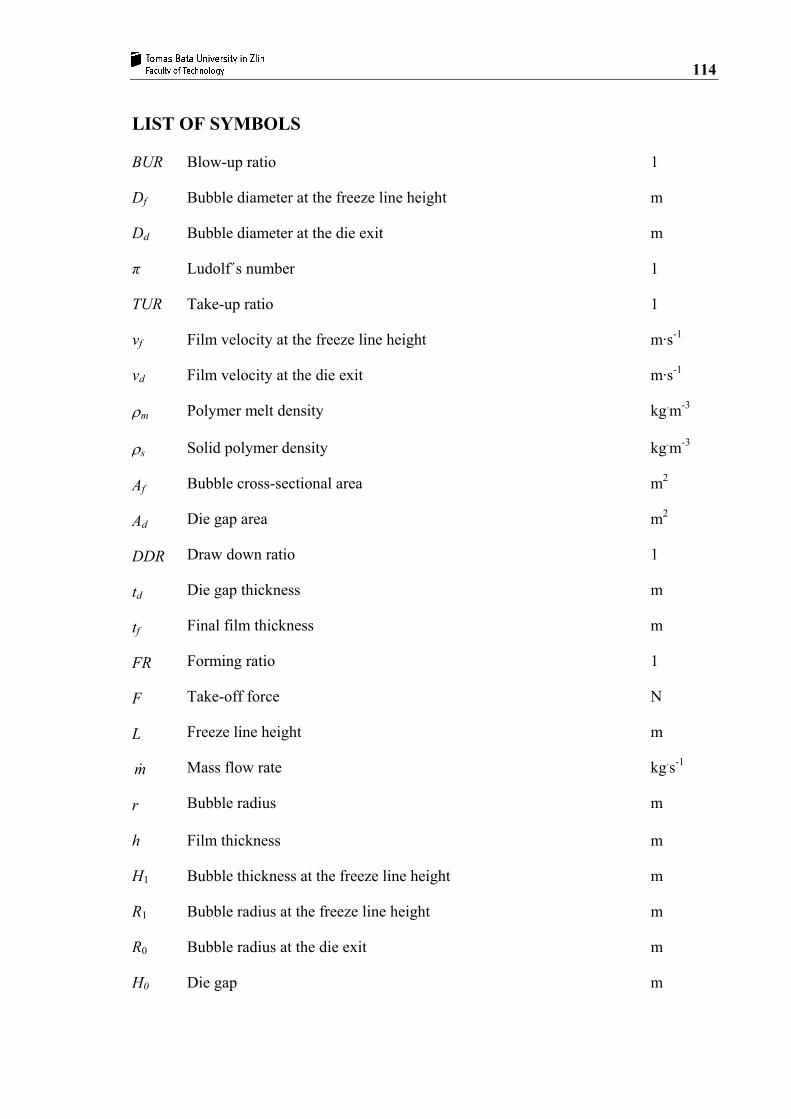
114
LIST OF SYMBOLS
BUR
Df
Dd
π
TUR
vf
vd
ρm
Blow-up ratio
Bubble diameter at the freeze line height
Bubble diameter at the die exit
Ludolf´s number
Take-up ratio
Film velocity at the freeze line height
Film velocity at the die exit
Polymer melt density
1
m
m
1
1
m·s-1
m·s-1
kg.m-3
ρs
Af
Ad
DDR
td
tf
FR
F
L
m&
r
Solid polymer density
Bubble cross-sectional area
Die gap area
Draw down ratio
Die gap thickness
Final film thickness
Forming ratio
Take-off force
Freeze line height
Mass flow rate
Bubble radius
kg.m-3
m2
m2
1
m
m
1
N
m
kg.s-1
m
h Film thickness m
H1 Bubble thickness at the freeze line height m
R1 Bubble radius at the freeze line height m
R0 Bubble radius at the die exit m
H0 Die gap m

115
x1 Tangential direction m
x2 Thickness direction m
x3 Circumferential direction m
v Film velocity m·s-1
ρ Film density kg·m-3
Rg Universal gas constant J·K-1mol-1
T Bubble temperature K
P* Cohesion pressure Pa
w Molecular weight kg·mol-1
b´ Specific volume m3·kg-1
Δp Internal bubble pressure Pa
σ11 Tangential component of the total stress tensor Pa
Rm Curvature radius m
σ33 Circumferential component of the total stress tensor Pa
Rt Curvature radius m
Θ Bubble angle °
G Gravity N
H Force created by the air flow N
rf Bubble radius at the freeze line height m
dx Element length in x direction m
dr Element length in r direction m
σ Total stress tensor Pa
p Internal load Pa·m
I Unit tensor 1
τ Extra stress Pa
σ22 Thickness directions of the stress Pa

116
τ11 Extra stress in the tangential directions Pa
τ22 Extra stress in the thickness directions Pa
τ33 Extra stress in the circumferential directions Pa
J Membrane compliance Pa-1
y Equation for the bubble shape (radius) without the neck m
λ1 Lagrange multiplier Pa
pJ Film blowing model parameter m
φ Zatloukal-Vlcek model function 1
A Zatloukal-Vlcek model function 1
α´ Zatloukal-Vlcek model function 1
φ´´ Zatloukal-Vlcek model function 1
A´´ Zatloukal-Vlcek model function 1
α´´ Zatloukal-Vlcek model function 1
BUR0 Blow-up ratio at the neck 1
y1, y2 Equations for the bubble shape (radius) having the neck height m
L1 Neck height m
ξ Zatloukal-Vlcek model function m2
FI Tensile force acting at the die exit (Zatloukal-Vlcek model) N
FII Tensile force at the freeze line height (Zatloukal-Vlcek model) N
pL Force acting in the thickness direction N
Q Volumetric flow rate m3·s-1
η0 Newtonian viscosity Pa·s
D Deformation rate tensor s-1
FII,N Force acting at the freeze line height (Newton model) N
A‘ Zatloukal-Vlcek model function 1
p’J‘ Film blowing model parameter m
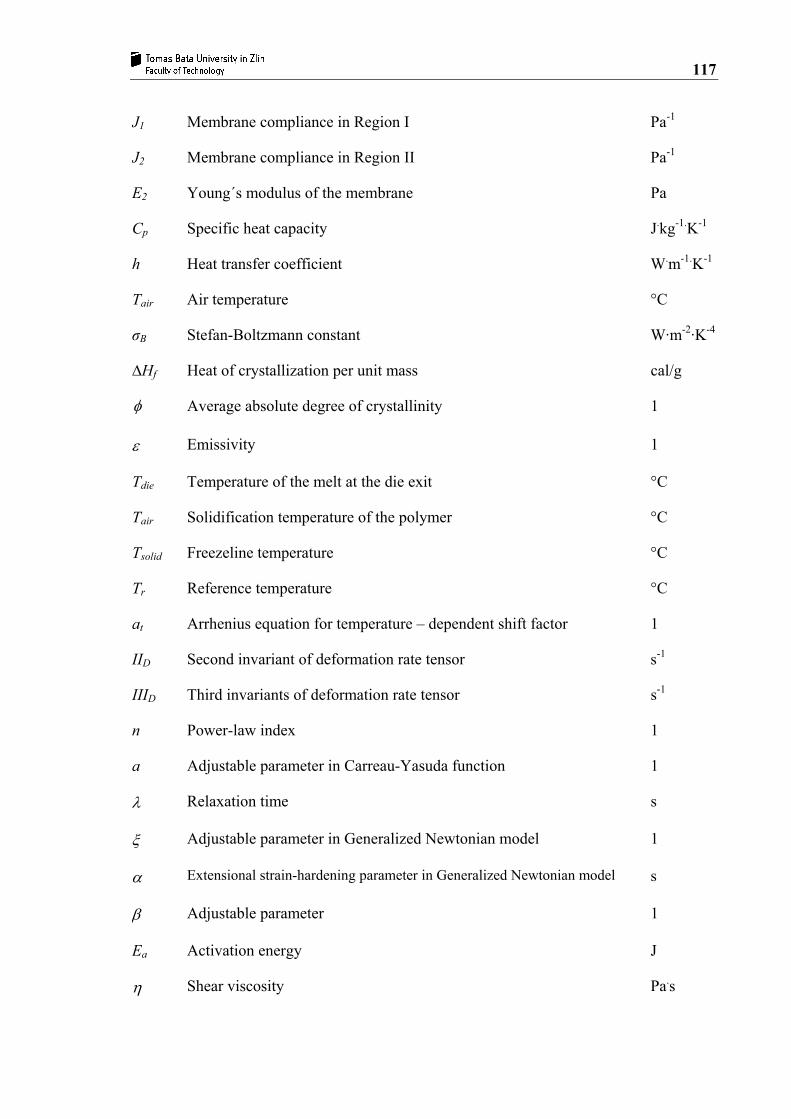
117
J1 Membrane compliance in Region I Pa-1
J2 Membrane compliance in Region II Pa-1
E2 Young´s modulus of the membrane Pa
Cp Specific heat capacity J.kg-1.K-1
h Heat transfer coefficient W.m-1.K-1
Tair Air temperature °C
σB Stefan-Boltzmann constant W·m-2·K-4
∆Hf Heat of crystallization per unit mass cal/g
φ Average absolute degree of crystallinity 1
ε Emissivity 1
Tdie Temperature of the melt at the die exit °C
Tair Solidification temperature of the polymer °C
Tsolid Freezeline temperature °C
Tr Reference temperature °C
at Arrhenius equation for temperature – dependent shift factor 1
IID Second invariant of deformation rate tensor s-1
IIID Third invariants of deformation rate tensor s-1
n Power-law index 1
a Adjustable parameter in Carreau-Yasuda function 1
λ Relaxation time s
ξ Adjustable parameter in Generalized Newtonian model 1
α Extensional strain-hardening parameter in Generalized Newtonian model s
β Adjustable parameter 1
Ea Activation energy J
η Shear viscosity Pa.s

118
ηE Extensional viscosity Pa.s
η Bubble viscosity Pa.s
ε& Extensional rate s-1
v velocity mean value along the bubble m.s-1
h thickness mean value along the bubble m

119
LIST OF FIGURES
Fig. 1. Film blowing line ..................................................................................................... 12
Fig. 2. Procedure used to start the film blowing process .................................................... 13
Fig. 3. Elements of blown film ............................................................................................. 15
Fig. 4. Draw resonance ....................................................................................................... 20
Fig. 5. Helical instability ..................................................................................................... 20
Fig. 6. FLH instability ......................................................................................................... 21
Fig. 7. Bubble sag ................................................................................................................ 22
Fig. 8. Bubble flutter ............................................................................................................ 23
Fig. 9. Bubble breathing ...................................................................................................... 23
Fig. 10. Bubble tear ............................................................................................................. 24
Fig. 11. Effect of mass flow rate on the film blowing stability (LDPE material,
FLH = 250mm, Tmelt = 185oC) [27]. Note that unstable area occurs below the
stability contours. ....................................................................................................... 25
Fig. 12. The effect of FLH on the film blowing stability (LLDPE material, mass flow
rate is 2kg/h, Tmelt = 187oC) [27]. Note that unstable area occurs below the
stability contours and vice versa. ............................................................................... 26
Fig. 13. Effect of melt temperature on the film blowing instability (LLDPE material,
FLH = 250mm, mass flow rate = 2kg/h) [27]. Note that unstable area occurs
below the stability contours. ....................................................................................... 27
Fig. 14. Cooling system ....................................................................................................... 28
Fig. 15. Single lip design ..................................................................................................... 30
Fig. 16. Dual lip design ....................................................................................................... 31
Fig. 17. IBC system .............................................................................................................. 32
Fig. 18. Venturi effect .......................................................................................................... 33
Fig. 19. Venturi and Coanda effects .................................................................................... 33
Fig. 20. Stabilization by iris ................................................................................................. 34
Fig. 21. Bubble guides – type A ........................................................................................... 35
Fig. 22. Bubble guides – type B ........................................................................................... 36
Fig. 23. Bubble calibration cage ......................................................................................... 37
Fig. 24. Film blowing variables ........................................................................................... 41
Fig. 25. Cartesian coordinate system .................................................................................. 42
Fig. 26. Membrane before deformation .............................................................................. 45

120
Fig. 27. Membrane after deformation ................................................................................. 45
Fig. 28. Bubble without neck [2]. Left side represents measurements, right hand side
represents prediction. ................................................................................................. 47
Fig. 29. Bubble with neck – shape and acting forces .......................................................... 50
Fig. 30. Bubble with the neck [2]. Left side represents measurements, right hand side
represents prediction. ................................................................................................. 50
Fig. 31. High stalk bubble – shape and acting forces ......................................................... 52
Fig. 32. High stalk bubble [6]. Left side represents measurements, right hand side
represents prediction. ................................................................................................. 53
Fig. 33. Film blowing experimental set-up. 33a) General view of the experimental
film blowing line; 33b) Closer view of the film blowing die; 33c) Used spiral
mandrel. ...................................................................................................................... 64
Fig. 34. The experimentally determined stability contours for both, linear and
branched metallocene LLDPE samples (FLH 180mm and temperature 190°C). ...... 65
Fig. 35. Rheology data for tested resins taken from [57]; 35a) Complex viscosity
data for three mLLDPEs having different levels of long chain branching
obtained experimentally by ARES rotational rheometer at 140oC; 35b) Time-
dependent uniaxial extensional viscosity ( )tE+η data for three mLLDPEs having
different levels of long chain branching obtained by SER at 140oC. ......................... 66
Fig. 36. Comparison between generalized Newtonian model fitting lines and
experimental data for LDPE material taken from Tas's Ph.D. thesis [1]. ................. 86
Fig. 37. Comparison between Zatloukal-Vlcek model predictions and experimental
data for the LDPE bubble shape taken from Tas's Ph.D. thesis [1]. ......................... 87
Fig. 38. Comparison between non-Newtonian Zatloukal-Vlcek model predictions and
experimental data for the LDPE bubble velocity taken from Tas's Ph.D. thesis
[1]. .............................................................................................................................. 88
Fig. 39. Comparison between non-Newtonian Zatloukal-Vlcek model predictions and
experimental data for the LDPE bubble temperature taken from Tas's Ph.D.
thesis [1]. .................................................................................................................... 89
Fig. 40. Typical processing window predicted by the Zatloukal-Vlcek model for
non-isothermal processing conditions and non-Newtonian polymer melt. ................ 90
Fig. 41. Stability contours for different level of the Newtonian viscosity predicted by
the Zatloukal-Vlcek model for non-isothermal processing conditions and non-

121
Newtonian polymer melt. Model and machine stability contours are
represented by triangles and circles, respectively. ................................................. 91
Fig. 42. Stability contours for different level of the heat transfer coefficient predicted
by the Zatloukal-Vlcek model for non-isothermal processing conditions and
non-Newtonian polymer melt. Model and machine stability contours are
represented by triangles and circles, respectively. ................................................. 92
Fig. 43. Stability contours for different level of the internal bubble pressure
predicted by the Zatloukal-Vlcek model for non-isothermal processing
conditions and non-Newtonian polymer melt. Model, machine and
circumference stability contours are represented by triangles, circles and
squares, respectively. ................................................................................................. 93
Fig. 44. Stability contours for different level of the rupture stress predicted by the
Zatloukal-Vlcek model for non-isothermal processing conditions and non-
Newtonian polymer melt. Model and machine stability contours are
represented by triangles and circles, respectively. ................................................. 94
Fig. 45. Stability contours for different level of the die radius predicted by the
Zatloukal-Vlcek model for non-isothermal processing conditions and non-
Newtonian polymer melt. Model and machine stability contours are
represented by triangles and circles, respectively. ................................................... 95
Fig. 46. Stability contours for different level of the mass flow rate predicted by the
Zatloukal-Vlcek model for non-isothermal processing conditions and non-
Newtonian polymer melt. Model and machine stability contours are
represented by triangles and circles, respectively. ................................................... 96
Fig. 47. Stability contours for different level of the melt/die temperature predicted by
the Zatloukal-Vlcek model for non-isothermal processing conditions and non-
Newtonian polymer melt. Model and machine stability contours are
represented by triangles and circles, respectively. ................................................... 97
Fig. 48. Stability contours for different level of the cooling air temperature predicted
by the Zatloukal-Vlcek model for non-isothermal processing conditions and
non-Newtonian polymer melt. Model and machine stability contours are
represented by triangles and circles, respectively. ................................................... 98
Fig. 49. Stability contours for different level of the power law index (index of
non-Newtonian behavior) predicted by the Zatloukal-Vlcek model for non-

122
isothermal processing conditions and non-Newtonian polymer melt. Model and
machine stability contours are represented by triangles and circles,
respectively. ................................................................................................................ 99
Fig. 50. Stability contours for different level of the flow activation energy predicted
by the Zatloukal-Vlcek model for non-isothermal processing conditions and
non-Newtonian polymer melt. Model and machine stability contours are
represented by triangles and circles, respectively. ................................................. 100
Fig. 51. Shear viscosity prediction of the generalized Newtonian model for different
values of η0 and λ (effect of Mw). ............................................................................ 101
Fig. 52. Predicted film blowing stability contours for three virtual materials (Fig. 51)
by using Zatloukal-Vlcek film blowing model (effect of Mw). Processing
conditions are provided in Tab. 20. ........................................................................ 102
Fig. 53. Shear and extensional viscosity prediction of the generalized Newtonian
model for different values of ξ (different level long chain branching). .................... 103
Fig. 54. Predicted film blowing stability contours for five virtual materials (Fig. 53)
by using Zatloukal-Vlcek film blowing model (effect of long chain branching).
Processing conditions are provided in Tab. 20. ....................................................... 104
Fig. 55. Shear and extensional viscosity prediction of the generalized Newtonian
model for different values of α (different level long chain branching). ................... 105
Fig. 56. Predicted film blowing stability contours for five virtual materials (Fig. 55)
by using Zatloukal-Vlcek film blowing model (effect of long chain branching).
Processing conditions are provided in Tab. 20. ....................................................... 106
Fig. 57. Shear and extensional viscosity prediction of the generalized Newtonian
model for different (linear and branched) mLLDPE polymers (different level
long chain branching is introduced by varying of α parameter). ............................ 107
Fig. 58. Comparison between experimental data taken from [54] and predicted film
blowing stability contours (lines) for linear and branched mLLDPE polymers
(Fig. 57) by using Zatloukal-Vlcek film blowing model. Model parameters are
provided in Tabs. 20-21. ........................................................................................... 108

123
LIST OF TABLES
Tab. 1. The effect of major process variables on bubble geometry. .................................... 17
Tab. 2. Summary and description of the constitution equations for the solution of the
film blowing process (adapted from [34]). ................................................................ 38
Tab. 3. A full set of the Pearson and Petrie equations. ....................................................... 42
Tab. 4. Summary of the Zatloukal-Vlcek model for the bubble without neck. ..................... 46
Tab. 5. Parameters A and φ for different bubble shapes (y). Parameters A´, A´´ are
equal to A and parameters φ´, φ´´ are the same as φ [2]. .......................................... 47
Tab. 6. Zatloukal-Vlcek model for the bubble with the neck. .............................................. 48
Tab. 7. Zatloukal-Vlcek model for the high stalk bubble. .................................................... 51
Tab. 8. The stability contour equations. .............................................................................. 54
Tab. 9. Zatloukal-Vlcek model parameters used in the model testing on the Tas's
Ph.D. thesis data for LDPE. ....................................................................................... 67
Tab. 10. Summarization of the calculated data in the Fig. 41 for Newtonian viscosity
effect analysis (Q = 15.09168·10-7 m3·s-1)................................................................... 75
Tab. 11. Summarization of the calculated data in the Fig. 42 for the heat transfer
effect analysis (Q = 15.09168·10-7 m3·s-1)................................................................... 76
Tab. 12. Summarization of the calculated data in the Fig. 43 for the internal bubble
pressure analysis (Q = 15.09168·10-7 m3·s-1). ............................................................ 77
Tab. 13. Summarization of the calculated data in the Fig. 44 for the melt
strength/melt rupture effect analysis (Q = 15.09168·10-7 m3·s-1). .............................. 78
Tab. 14. Summarization of the calculated data in the Fig. 45 for the die radius effect
analysis (Q = 15.09168·10-7 m3·s-1). ........................................................................... 79
Tab. 15. Summarization of the calculated data in the Fig. 46 for the mass flow rate
effect analysis. ............................................................................................................ 80
Tab. 16. Summarization of the calculated data in the Fig. 47 for the die /melt
temperature effect analysis (Q = 15.09168·10-7 m3·s-1). ............................................. 81
Tab. 17. Summarization of the calculated data in the Fig. 48 for the cooling air
temperature effect analysis (Q = 15.09168·10-7 m3·s-1). ............................................. 82
Tab. 18. Summarization of the calculated data in the Fig. 49 for power law index
effect analysis (Q = 15.09168·10-7 m3·s-1)................................................................... 83
Tab. 19. Summarization of the calculated data in the Fig. 50 for the flow activation
effect analysis (Q = 15.09168·10-7 m3·s-1)................................................................... 84

124
Tab. 20. Zatloukal-Vlcek film blowing model parameters including Newtonian
viscosity, η0, for generalized Newtonian constitutive equation. ................................. 85
Tab. 21. Parameters of the generalized Newtonian constitutive equation. ......................... 85

125
LIST OF APPENDICES
APPENDIX A 1: Film blowing process
APPENDIX A 2: CD-ROM

AN
NU
LAR
DIE
TAB
LE F
LAP
APPENDIX P I: FILM BLOWING PROCESS
CA
LIB
RA
TIO
N C
AG
E
PO
SIT
ION
-CO
NTR
OL
DR
AW
RE
GU
LATI
ON
CA
LIB
RA
TIO
N C
AG
E
AV
ER
AG
E-R
EG
ULA
TIO
N
FILM
AV
ER
AGE
C
ON
TRO
L
GU
IDE
RO
LL
AIR
RE
GU
LATI
ON
AIR
(CO
OLI
NG
) RIN
G
EX
TRU
DE
R
FILM
CA
LIB
RA
TIO
N C
AG
E
NIP
RO
LLS
FILM
WID
TH
CO
NTR
OL
FILM
TH
ICK
NE
SS
C
ON
TRO
L
MIC
RO
-P
RO
CE
SS
OR
FILM
CH
AM
BE
R
CR
OS
S C
UTT
ING
M
EC
HA
NIS
M
WIN
D-U
P
DE
VIC
E A
IR IN
LET