non-linear extrapolation of laminar flame properties from...

Paper # 087LF-0020 Topic: Laminar Flame

Western States Section of the Combustion InstituteCalifornia Institute of Technology

March 23-25, 2014.

Non-linear Extrapolation of Laminar Flame Properties fromSpherically Expanding Flames

S. Coronel1, N. Bitter1, V. Thomas 2, R. Mevel∗1, J.E. Shepherd1

1Graduate Aeronautics Laboratory (GALCIT),California Institute of Technology, Pasadena, California 91125, USA

2Mechanical Engineering,Johns Hopkins University, Baltimore, MD 21218

The spherically expanding flame is a useful configuration for experimentally measuring laminar flamespeeds and Markstein lengths. Although these parameters are often fitted to the data linearly, for highlystretched flames it can be necessary to employ a fitting procedure that accounts for nonlinearity ofthe relationship between flame speed and stretch rate. This paper assesses the performance of suchmethods by generating sets of synthetic data and then attempting to recover the laminar flame speed andMarkstein length using a nonlinear fit. The method used in this paper fits the laminar flame properties byminimizing the difference between the data points and a simulated flame trajectory, using a non-linearleast squares method to accomplish the minimization. It is found that the least squares error, which is tobe minimized, is a weak function of the Markstein length and exhibits a shallow minimum, especiallyfor noisy data. This can lead to substantial error in the fitted value of the Markstein length; for instance,2% noise in the flame radius data produces about 20% relative error in the fitted Markstein length. Theinitial and final flame radii as well as the number of points in the experimental data set are found tohave only a small influence on the results. However, the results are sensitive to the initial guesses thatare used to start the least squares minimization. Finally we observe that for positive Markstein lengththere is an upper limit to the nonlinear relationship between flame speed and stretch, and fitting canbecome inaccurate near this limit. Despite these difficulties, the nonlinear fitting approach performsconsiderably better than linear ones for highly stretched flames.

1 Introduction

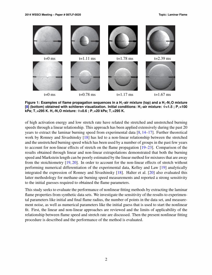
Laminar flame properties such as the laminar burning speed and the Markstein length are importantfundamental parameters for a wide number of combustion applications including spark ignitionengines [1] and gas turbines [2]. Knowledge of the laminar burning speed is also important inmodeling turbulent combustion since the turbulent burning speed is often modeled as a function ofthe laminar burning speed [3, 4]. The laminar burning speed is defined as the normal propagationvelocity of fresh gas relative to a fixed, planar flame front; it is frequently measured experimentallyusing spherically expanding flames [5–7]. Figure 1 shows examples of spherical flame propagationin hydrogen-based mixtures. The presence of flame stretch in such experiments precludes directmeasurement of the laminar burning velocity [9]. Instead, the measured flame velocity must beextrapolated to conditions of zero stretch. Markstein first proposed this correction to the burningspeed by introducing a parameter now known as the Markstein length [10], which characterizesthe response of the flame to stretch. Asymptotic theoretical analysis [11–13] performed in the limit

1

2014 WSSCI Meeting – Paper # 087LF-0020 Topic: Laminar Flame

t=0 ms t=1.11 ms t=1.78 ms t=2.39 ms

t=0 ms t=0.78 ms t=1.17 ms t=1.67 ms

Figure 1: Examples of flame propagation sequences in a H2-air mixture (top) and a H2-N2O mixture[8] (bottom) obtained with schlieren visualization. Initial conditions: H2-air mixture: Φ=1.5 ; P1=100kPa; T1=295 K. H2-N2O mixture: Φ=0.6 ; P1=20 kPa; T1=295 K.

of high activation energy and low stretch rate have related the stretched and unstretched burningspeeds through a linear relationship. This approach has been applied extensively during the past 20years to extract the laminar burning speed from experimental data [8, 14–17]. Further theoreticalwork by Ronney and Sivashinsky [18] has led to a non-linear relationship between the stretchedand the unstretched burning speed which has been used by a number of groups in the past few yearsto account for non-linear effects of stretch on the flame propagation [19–23]. Comparison of theresults obtained through linear and non-linear extrapolations demonstrated that both the burningspeed and Markstein length can be poorly estimated by the linear method for mixtures that are awayfrom the stoichiometry [19, 20]. In order to account for the non-linear effects of stretch withoutperforming numerical differentiation of the experimental data, Kelley and Law [19] analyticallyintegrated the expression of Ronney and Sivashinsky [18]. Halter et al. [20] also evaluated thislatter methodology for methane-air burning speed measurements and reported a strong sensitivityto the initial guesses required to obtained the flame parameters.

This study seeks to evaluate the performance of nonlinear fitting methods by extracting the laminarflame properties from synthetic data sets. We investigate the sensitivity of the results to experimen-tal parameters like initial and final flame radius, the number of points in the data set, and measure-ment noise, as well as numerical parameters like the initial guess that is used to start the nonlinearfit. First, the linear and non-linear approaches are reviewed and the limits of applicability of therelationship between flame speed and stretch rate are discussed. Then the present nonlinear fittingprocedure is described and the performance of the method is evaluated.

2


2 Methodologies to extract flame properties

2.1 Linear methodology

Asymptotic theoretical analysis by Sivashinsky [11], Matalon and Matkowsky [12] and Clavin[13], performed in the limit of high activation energy, reveals a linear relation between the stretchedand unstretched burning speeds in the low stretch rate regime

SL = S0L − L

′

B ·K. (1)

Here SL and S0L are the stretched and the unstretched laminar burning speeds, L′

B is the unburntgas Markstein length and K is the stretch rate. Karlovitz et al. [24] expressed the stretch rate interms of the normalized rate of change of an elementary flame front area as

K =1

A· dAdt, (2)

where A the flame front area. In the case of a spherical flame, the flame surface is given by

A = 4 · π ·R2f , (3)

which leads to the following expression for the stretch rate [7, 9, 14, 17]:

K = 2 · VSRf

, (4)

given that the stretched spatial velocity, or the flame speed, VS , corresponds to the flame radiusincrease rate

VS =dRf

dt. (5)

In the case of a large volume vessel and for measurements limited to the initial period of prop-agation where the flame radius is small, the pressure increase can be neglected [25], so that theburning speed and the spatial velocity are linked only through the expansion ratio across the flamefront

SL =VSσ. (6)

where σ is the expansion ratio defined as

σ =ρuρb, (7)

and ρu and ρb are the unburnt and burnt gas densities, respectively. Combining Equation 1 andEquation 6, the stretched and unstretched flame speed can be linked

VS = V 0S − LB ·K, (8)

where LB=L′B/σ. Using the experimental evolution of the flame radius as a function of time, the

local flame velocity as well as the local stretch rate can be derived and the unstretched flame speedobtained by linearly extrapolating to zero stretch. As a part of this procedure one must fit the

3


Rf = f(t) data, usually with a high order polynomial, and differentiate the fitted curve in order toobtain a smooth evolution of the flame speed as a function of stretch. The main limitation of thisprocedure arises from the differentiation which introduce artificial noise that can lead to misleadingresults.

Another way to proceed is to substitute Equation 4 and Equation 6 into Equation 1, and integratewith respect to time, which produces an expression for the unstretched spatial flame velocity as afunction of time and flame radius

V 0S · (ti − t) = Ri

f −Rf + 2 · LB · ln

(Rf

Rif

)+ Cst (9)

Here the superscript i designates the ith data point in a set of experimental measurements, and Cstis an integration constant. Using Equation 9, a least square fitting procedure can be applied to anexperimental set of Rf = f(t) data provided that Rf � Dexp, where Dexp is the characteristicdimension of the experimental set-up. The unstretched flame velocity and the Markstein length aredetermined from this procedure as the coefficients of the linear fit.

2.2 Non-linear methodology

By removing the assumption of a linear relationship between the stretched and the unstretchedflame speeds, Ronney and Sivashinsky [11] obtained the nonlinear result:(

VSV 0S

)2

ln

(VSV 0S

)2

= −2σLBK

V 0S

(10)

This expression can be used directly to derive both the flame speed and the Markstein length, butin doing so one must fit the Rf = f(t) data with polynomials and differentiate to determine Vs, aswas done by Halter et al. [20] and Bouvet et al. [22].

In order to avoid differentiating the experimental data, Kelley and Law [19] proposed an integralform of Equation 10

t = A

[E1

(ln ξ2

)− 1

ξ2 ln ξ

]+ C (11)

whereA =

2σLB

V 0S

, (12)

Rf = −2σLB

ξ ln ξ, (13)

E1 (x) =

∫ ∞x

e−z

zdz, (14)

andC is a constant of integration. The parameter ξ, which is the ratio of the stretched to unstretchedflame speed, falls in the range [e−1, 1) for LB > 0 and [1,∞) for LB < 0. The parameters, A, LB,

4


and C can be determined using non-linear least-squares fitting, that is, minimizing the expression

ER =1

N

[N∑i=0

(ti − A

[E1

(ln ξ2i

)− 1

ξ2i ln ξi

]− C

)2]1/2

(15)

where the summation on i is taken over all measured values of flame radius and time. The un-stretched flame speed can then be deduced from the values of A and LB that minimize Equation 15.

3 Analysis of the Ronney-Sivashinsky non-linear equation

The nonlinear method of flame speed extraction described in section 2 relies on the quasi-steadyrelationship between flame speed and stretch rate given by Equation 10. However, this equationhas solutions only for certain values of the ratio σLB/Rf . To demonstrate this, one can combineEquation 4 with Equation 10 and simplify the logarithmic term to obtain the relation

VSV 0S

· ln(VSV 0S

)= −2σLB

Rf

. (16)

Since the burning velocity is positive, the term on the left hand side may take on values only withinthe range [−e−1,∞). For LB < 0 there is one solution for all positive values ofRf , but for LB > 0there are solutions only if

Rf

2σLB

≥ e (LB > 0) (17)

Thus for positive Markstein length there exists a minimum flame radius below which the quasi-steady relationship between flame speed and stretch rate is not valid, and hence the laminar flamespeed cannot be extracted using Equation 10. This constraint can also be viewed as a maximumMarkstein length, LB,max, for fixed flame radius. The fact that no solutions exist for small flameradii is a consequence of the neglected unsteady term, which is important in the early flame dy-namics [11].

When extracting laminar flame properties from experimental data, one can apply the methods ofsection 2 only for data points having large enough flame radii to satisfy Equation 17. Data pointswhich do not satisfy this criterion do not conform to the model equation, Equation 10, and thus maylead to a poor quality of fit (large residuals) or erroneous fitted values of V 0

s and LB. Unfortunately,the limitation given by Equation 17 depends on the Markstein length, which is itself one of theunknowns being sought. In practice one must initially select the experimental data points based onan estimate of LB and confirm after fitting the data that Equation 17 was indeed satisfied, revisingthe set of included data points if necessary.

4 Description of the present approach

The majority of previous studies [20,26] that have studied the accuracy of the linear and nonlinearmethods for flame parameters extraction have used experimental data. A difficulty of this approachis that the exact flame speed and Markstein length are not known a priori and depend on the

5


method used to obtain them. Another approach is to use synthetic data, as was done by Chen [27].However, Chen generated his reference data using detailed numerical simulations which limits thenumber of synthetic samples that can be generated because of the high computational cost of suchsimulations. In this paper, synthetic data is generated instead by numerically integrating the flameradius as a function of time, evaluating the flame speed at each time step using Equation 16.

The present method for extracting LB and V 0S uses non-linear least squares regression to determine

the values of LB and V 0S that minimize the difference between the experimentally measured flame

radius, Rif , and an ideal flame spherical flame radius, Ri

f,calc, which represents the evolution ofspherical flame in the absence of noise and measurement error for a flame that obeys Equation 16.The values of LB and V 0

S are extracted by minimizing the residual function,

ER =1

N

N∑i=1

(Ri

f −Rif,calc

Rif

)21/2

(18)

The first step in the process is to generate an idealized set of data points, ti vs. Rif,calc, by inte-

grating Equation 16. The initial conditions, t0 and R0f , are determined from the data set to be

fitted. The values of LB and V 0S are then iteratively refined until Equation 18 is minimized. The

numerical integration of Equation 16 is carried out using the Matlab ODE solver ode15i and thenonlinear least squares minimization is accomplished using the Levenberg-Marquardt algorithmas implemented in the Matlab function lsqnonlin.

5 Results and discussion

5.1 Objective Function

The proposed nonlinear fitting method involves the minimization of an objective function givenby Equation 18. The rate of convergence, sensitivity to noise, and robustness of this procedureall depend on the behavior of the objective function for which the minimum is being sought. Anexample of the objective function is shown in Figure 2; the plot was created by generating syntheticdata points of flame radius vs. time for LB = −1 mm and V 0

s = 300 mm/s and then evaluating theresidual, Equation 18, for other values of the Markstein length and burning velocity. This residual(on a logarithmic scale) is indicated by the contours in Figure 2, and it is seen that the residual isminimized at the correct solution point. However the minimum in the objective function is ratherelongated, that is, the solution point is much less sensitive to the Markstein length than to theunstretched burning velocity. Note that the apparent multiple local minima on the contour plot areartifacts of the contouring algorithm; the surface does in fact smoothly approach a single solutionpoint.

Slices through the contour plot in Figure 2(a) for three values of the Markstein length are shownin Figure 2(b). In addition, noise in the experimental measurement of the flame radius has beensimulated by adding random perturbations to each value of the flame radius; the magnitude of theadded noise was take to be 0%, 1%, 2%, or 5% of the instantaneous flame radius. The objectivefunction does exhibit a local minimum at the correct solution, but the depth of the minimum andthe slope in its vicinity are reduced somewhat when noise is added. For the higher noise levels

6


LB (mm)

VS0 (

mm

/s)

−2 −1.5 −1 −0.5 0200

220

240

260

280

300

320

340

360

380

400

Log(

ER

) (m

m)

−8

−7

−6

−5

−4

−3

−2

−1

0

1

200 220 240 260 280 300 320 340 360 380 400−6

−5

−4

−3

−2

−1

0

1

VS0 (mm/a)

Log(

ER

) (m

m)

LB = −2 mm, 0%

LB = −1 mm, 0%

LB = 0 mm, 0%

LB = −2 mm, 1%

LB = −1 mm, 1%

LB = 0 mm, 1%

LB = −2 mm, 2%

LB = −1 mm, 2%

LB = 0 mm, 2%

LB = −2 mm, 5%

LB = −1 mm, 5%

LB = 0 mm, 5%

(a) (b)

Figure 2: a) Contour plot of the objective function (Equation 18) for various values of Marksteinlength and unstretched burning velocity. The actual solution is LB = −1 mm, V 0

s = 300 mm/s. Con-tours levels are the base 10 logarithm of the objective function. b) Slices through the contour plotfor Markstein lengths of -2, -1, and 0 mm. Random noise has been included by adding 0%, 1%, 2%,or 5% relative error to each flame radius data point.

the minimum is quite shallow; however, the nonlinear fitting method is still able to converge tothe correct solution. Other noise models have also been employed including noise of uniformmagnitude and noise that decreases with increasing flame radius; the results from those modelswere nearly indistinguishable from those shown in Figure 2(b).

The elongated shape of the minimum in the objective function is not a property of the new methodalone, but is shared by both the linear method and the nonlinear method of Kelley and Law [19](see section 2). These two methods also rely on least squares fitting by minimizing objectivefunctions derived from Equation 9 and Equation 15, respectively. Contours of these two objectivefunctions for the same conditions as Figure 2 are shown in Figure 3. Although the amplitudes of theresiduals differ since each method minimizes a slightly different quantity, the qualitative behaviorof all three methods is similar. Note, however, that the minimum for linear method deviates fromthe actual solution of LB = −1 mm, V 0

s = 300 mm/s because the flame is slightly outside of thelinear stretch regime.

5.2 Performance of the present method

In order to evaluate the performance of the Levenberg-Marquardt, synthetic tsyn vs Rf,syn datawere generated using Equation 16 with LB and V 0

S values in the range LB ∈ [−5.0, LB,max] mm

whereLB,max =R0

f

2eand V 0

S ∈ [300, 35000] mm/s, which are representative of typical hydrocarbon-air and hydrogen-air mixtures. The choice of LB,max is based on the limit of Equation 16 describedin section 3. After generating the synthetic data, an attempt was made to recover the laminar flameparameters from the synthetic data using a random set of initial guesses for LB and V 0

S . The effect

7


LB [mm]

Vs0 [m

m/s

]Contours of log

10(residual): L

b = −1.00 mm, V

s0 = 300 mm/s

−2 −1.5 −1 −0.5 0200

220

240

260

280

300

320

340

360

380

400

−5

−4.5

−4

−3.5

−3

−2.5

−2

−1.5

−1

−0.5

0

LB [mm]

Vs0 [m

m/s

]

Contours of log10

(residual): Lb = −1.00 mm, V

s0 = 300 mm/s

−2 −1.5 −1 −0.5 0200

220

240

260

280

300

320

340

360

380

400

−5

−4.5

−4

−3.5

−3

−2.5

−2

−1.5

−1

−0.5

0

Figure 3: Contour plots of the objective function for Kelley and Law’s method (left) and the linearmethod (right). The actual solution is LB = −1 mm, V 0

s = 300 mm/s.

of the number of points in the data set, the initial and final radii, and the initial guesses of LB andV 0S on the performance of the method have been considered. In addition, noise was added to the

synthetic data to assess its effect on the robustness of the method. The performance of the methodis judged in terms of the final value of the residual, ER, as well as in terms of the error of the fittedvalues of LB and V 0

S . These errors are calculated using Equation 19 and Equation 20.

EV 0S=V 0S,syn − V 0

S,calc

V 0S,syn

(19)

ELB=LB,syn − LB,calc

LB,syn

(20)

Figure 4 shows examples of synthetic data sets characterized by positive Markstein lengths. Thesets are generated using 100 points. In each case, both the correct values of the laminar burningspeed and of the Markstein length were obtained by applying the non-linear least squares fittingprocedure. The quality of the fitting is evident in the graphs presenting the evolution of the burningspeed as a function of stretch rate.

5.2.1 Effect of data set properties

The effect on convergence was studied by varying parameters such as the initial flame radius, R0f ,

final flame radius, Rfinalf and the size of the data set, N . To study the effect of N on convergence,

data sets of tsyn vs Rf,syn were generated based on the following parameters: R0f = 10 mm,

Rfinalf = 58 mm, N = [30, 50, 100]. The N values represent typical data set sizes obtained from

8


0 0.02 0.04 0.06 0.08 0.1 0.12 0.14 0.160

50

100

150

200

250

300

350

400

450

500

time (s)

radi

us (

mm

)

V

S0 = 3000 mm/s, L

B = 0.5 mm

VS0 = 2000 mm/s, L

B = 1.0 mm

VS0 = 1000 mm/s, L

B = 1.8 mm

0 200 400 600 800 1000 12000

500

1000

1500

2000

2500

3000

κ (1/s)

Fla

me

Spe

ed (

mm

/s)

VS0 = 3000 mm/s, L

B = 0.5 mm

VS0 = 2000 mm/s, L

B = 1.0 mm

VS0 = 1000 mm/s, L

B = 1.8 mm

Figure 4: Examples of synthetic data and non-linear least-square regression curves obtained usingthe present numerical method. Both Rf,syn = f (tsyn) and V 0

S = f (κ) are presented.

experiments, where the size varies according to the framing rate of camera that is being used toacquire the flame images, the initial energy deposition used to ignite the mixture, and the typeof mixture used; faster flames lead to less images and vice-versa. The non-linear least squaressolver goes through 10 initial guesses of LB and 10 initial guesses of V 0

S , until the residual, ER,is minimized to the preset tolerance. The residual, ER, and errors, EV 0

Sand ELB

, are shown inFigure 5 as filled contours on a base 10 logarithmic scale.

The results shown in Figure 5 suggest that ER, EV 0S

, and ELBare insensitive to the size of the

data set, N . The figure also shows that ER, EV 0S

, and ELBincrease near the region of LB,max

indicated by the red contours, which is where the limit discussed in section 3 is approached. Forthe parameters tested, the results suggest that for the majority of Markstein lengths and flamespeeds the non-linear least squares fitting procedure will perform within the desired tolerances.

Next the effect of initial radius is studied, keeping the number of points in the data set fixedat N = 100. Data sets of tsyn vs Rf,syn were generated based on the following parameters:R0

f = [10, 15, 25] mm, Rfinalf = 58 mm. The non-linear least squares solver goes through 10

initial guesses of LB and 10 initial guesses of V 0S , until the residual, ER, is minimized to the preset

tolerance. The calculated errors, ELB, are shown in the left column of Figure 6 as filled contours

on a base 10 logarithmic scale. The scale on the x-axis increases when R0f increases since LB,max

is directly proportional to the initial flame radius. Visually there are small differences in the mag-nitude of the contours of ELB

for the R0f = 10 mm and R0

f = 15 mm cases; the differences suggestthat smaller errors are obtained for data sets with an initial flame radius of 10 mm than data setswith an initial flame radius of 15 mm. The 10 mm and 15 mm initial radius contours have a similarregion of concentrated high errors in the vicinity of LB,max. The 25 mm initial flame radius caseexhibits a larger concentration of high errors in the vicinity of LB,max than the other two initialflame radius cases.

To study the effect of Rfinalf on convergence, data sets of tsyn vs Rf,syn were generated based on

the following parameters: R0f = 10 mm, Rfinal

f = [25, 58, 80] mm. The non-linear least squares

9


solver goes through 10 initial guesses of LB and 10 initial guesses of V 0S , until the residual, ER,

is minimized to the preset tolerance. The calculated errors, ELB, are shown in the right column of

Figure 6 as filled contours on a base 10 logarithmic scale. The scale on the x-axis remains fixedsince R0

f is fixed for the three cases. There appears to be a change in the size of the region ofconcentrated high errors throughout the three cases. The size of the region decreases from the 25mm final flame radius case to the 58 mm final flame radius case, it then increases again to a largerregion of high errors in the 80 mm final flame radius case. Figure 6 suggests that there is an idealfinal flame radius that leads to a decrease in the size of the region of concentrated errors in LB.

LB (mm)

V0 S (mm

/s)

−5 −4 −3 −2 −1 0 1

0.5

1

1.5

2

2.5

3

3.5x 104

Log(

E R) (

mm

)

−15

−14

−13

−12

−11

−10

−9

−8

−7

−6

−5

−4

−3

−2

LB (mm)

V S0 (mm

/s)

−5 −4 −3 −2 −1 0 1

0.5

1

1.5

2

2.5

3

3.5x 104

Log(

E R) (

mm

)

−15

−14

−13

−12

−11

−10

−9

−8

−7

−6

−5

−4

−3

−2

LB (mm)

V S0 (mm

/s)

−5 −4 −3 −2 −1 0 1

0.5

1

1.5

2

2.5

3

3.5x 104

Log(

E R) (

mm

)

−15

−14

−13

−12

−11

−10

−9

−8

−7

−6

−5

−4

−3

−2

LB (mm)

V0 S (mm

/s)

−5 −4 −3 −2 −1 0 1

0.5

1

1.5

2

2.5

3

3.5x 104

Log(

|EL B|)

−15

−14

−13

−12

−11

−10

−9

−8

−7

−6

−5

−4

−3

−2

LB (mm)

V S0 (mm

/s)

−5 −4 −3 −2 −1 0 1

0.5

1

1.5

2

2.5

3

3.5x 104

Log(

|EL B|)

−15

−14

−13

−12

−11

−10

−9

−8

−7

−6

−5

−4

−3

−2

LB (mm)

V S0 (mm

/s)

−5 −4 −3 −2 −1 0 1

0.5

1

1.5

2

2.5

3

3.5x 104

Log(

|EL B|)

−15

−14

−13

−12

−11

−10

−9

−8

−7

−6

−5

−4

−3

−2

LB (mm)

V0 S (mm

/s)

−5 −4 −3 −2 −1 0 1

0.5

1

1.5

2

2.5

3

3.5x 104

Log(

|EV0 S|)

−15

−14

−13

−12

−11

−10

−9

−8

−7

−6

−5

−4

−3

−2

LB (mm)

V S0 (mm

/s)

−5 −4 −3 −2 −1 0 1

0.5

1

1.5

2

2.5

3

3.5x 104

Log(

|EV S0|)

−15

−14

−13

−12

−11

−10

−9

−8

−7

−6

−5

−4

−3

−2

LB (mm)

V S0 (mm

/s)

−5 −4 −3 −2 −1 0 1

0.5

1

1.5

2

2.5

3

3.5x 104

Log(

|EV S0|)

−15

−14

−13

−12

−11

−10

−9

−8

−7

−6

−5

−4

−3

−2

N = 30 N = 50 N = 100

Figure 5: Contour plots of ER, ELBand EV 0

Sfor N = [30, 50, 100]

10


LB (mm)

V S0 (mm

/s)

−5 −4 −3 −2 −1 0 1

0.5

1

1.5

2

2.5

3

3.5x 104

Log(

|EL B|)

−15

−14

−13

−12

−11

−10

−9

−8

−7

−6

−5

−4

−3

−2

−1

LB (mm)

V S0 (mm

/s)

−5 −4 −3 −2 −1 0 1

0.5

1

1.5

2

2.5

3

3.5x 104

Log(

|EL B|)

−15

−14

−13

−12

−11

−10

−9

−8

−7

−6

−5

−4

−3

−2

R0f = 10 mm, Rfinal

0 = 58 mm R0f = 10 mm, Rfinal

f = 25 mm

LB (mm)

V S0 (mm

/s)

−5 −4 −3 −2 −1 0 1 2

0.5

1

1.5

2

2.5

3

3.5x 104

Log(

|EL B|)

−15

−14

−13

−12

−11

−10

−9

−8

−7

−6

−5

−4

−3

−2

−1

LB (mm)

V S0 (mm

/s)

−5 −4 −3 −2 −1 0 1

0.5

1

1.5

2

2.5

3

3.5x 104

Log(

|EL B|)

−15

−14

−13

−12

−11

−10

−9

−8

−7

−6

−5

−4

−3

−2

R0f = 15 mm, Rfinal


f = 58 mm

LB (mm)

V0 S (mm

/s)

−4 −2 0 2 4

0.5

1

1.5

2

2.5

3

3.5x 104

Log(

|EL B|)

−15

−14

−13

−12

−11

−10

−9

−8

−7

−6

−5

−4

−3

−2

−1

LB (mm)

VS0 (

mm

/s)

−5 −4 −3 −2 −1 0 1

0.5

1

1.5

2

2.5

3

3.5x 10

4

Log(

|EL B

|)

−15

−14

−13

−12

−11

−10

−9

−8

−7

−6

−5

−4

−3

−2

R0f = 25 mm, Rfinal


f = 80 mm

Figure 6: Contour plots of ELBfor various initial radii (left) and various final radii (right).

11


5.2.2 Effect of the initial guess

In this section the sensitivity of the nonlinear least squares fit to the initial guesses of LB and V 0S

is explored. Synthetic data sets were generated using initial and final radii of R0f = 10 mm and

Rfinalf = 58 mm. The set of initial guesses was randomly generated for LB ∈ [−10, 10] mm and

V 0S ∈ [20, 100000] mm/s. For each pair of values of LB and V 0

S , either 1, 2, 5, or 10 different initialguesses were used. The contour plots in Figure 7 indicate that when only 1 initial guess of LB and1 initial guess of V 0

S are used, the error goes up as LB increases until the non-linear least squaressolver can no longer find a solution within a reasonable tolerance, this is indicated by the unfilledregion of the 1× 1 contour plot.

LB (mm)

VS0 (

mm

/s)

−5 −4 −3 −2 −1 0

0.5

1

1.5

2

2.5

3

3.5x 10

4

Log(

|EL B

|)

−15

−14

−13

−12

−11

−10

−9

−8

−7

−6

−5

−4

−3

−2

LB (mm)

VS0 (

mm

/s)

−5 −4 −3 −2 −1 0 1

0.5

1

1.5

2

2.5

3

3.5x 10

4

Log(

|EL B

|)

−15

−14

−13

−12

−11

−10

−9

−8

−7

−6

−5

−4

−3

−2

1× 1 2× 2

LB (mm)

VS0 (

mm

/s)

−5 −4 −3 −2 −1 0 1

0.5

1

1.5

2

2.5

3

3.5x 10

4

Log(

|EL B

|)

−15

−14

−13

−12

−11

−10

−9

−8

−7

−6

−5

−4

−3

−2

LB (mm)

V S0 (mm

/s)

−5 −4 −3 −2 −1 0 1

0.5

1

1.5

2

2.5

3

3.5x 104

Log(

|EL B|)

−15

−14

−13

−12

−11

−10

−9

−8

−7

−6

−5

−4

−3

−2

5× 5 10× 10

Figure 7: Contour plots of ELBfor four sets of initial guessues of LB and V 0

S

When the number of initial guesses is increased to 2 initial guesses of LB and 2 initial guessesof V 0

S , the solver is able to find a solution within the preset tolerances for the majority of the

12


domain shown in the 2 × 2 contour plot. As the number of initial guesses is increased further,the magnitude of ELB

decreases throughout the domain and the region of concentrated high errorsbecomes smaller, this is seen in the 5×5 and 10×10 contour plots in Figure 7. From this analysis,it is suggested that at least 10 initial guesses of LB and 10 initial guesses of V 0

S be chosen whenusing the non-linear least squares solver presented in this paper. If only 1 guess per parameter isto be used, then it is suggested that each guess be made on the basis of the linear least squares fit,Equation 9.

5.2.3 Effect of noise

The next step in this study was to investigate the robustness of the solver when noise was added tosynthetic data of Rf,syn. The addition of noise to Rf,syn is more representative of what is obtainedexperimentally when extracting flame radii from spherically propagating flame images. Data setsof tsyn vs Rf,syn were generated based on the following parameters: R0

f = 10 mm, Rfinalf = 58

mm. Noise proportional to the instantaneous flame radius was introduced to Rf,syn via a noisevector, e, that was randomly generated with values between -1 and 1. The resulting noisy syntheticdata sets, Rf,i are described by

Rf,i = Rf,syn ∗ [1 + i ∗ e] , (21)

where i is the noise percentage. The addition of 1% and 2% noise were studied, and example flameradius plots are shown in Figure 8.

1 1.5 2 2.5 3x 10−3

10

15

20

25

30

35

40

45

50

55

60

time (s)

radi

us (m

m)

OriginalWith Noise

1 1.5 2 2.5 3x 10−3

10

15

20

25

30

35

40

45

50

55

60

time (s)

radi

us (m

m)

OriginalWith Noise

1% noise 2% noise

Figure 8: Exact solutions and solutions with 1% and 2% noise for a case with LB = 1.8 mm andV 0S = 35000 mm/s.

The results of noise addition are shown in Figure 9, the figure is presented as synthetic LB vsfitted LB and the circle markers represent different values of V 0

S . The yellow markers indicate 0%noise addition, the red markers indicate 1% noise addition, the blue markers indicate 2% noiseaddition and the black dashed line indicates synthetic LB = calculated LB. Figure 9 shows that asthe noise percentage is increased, the calculated LB drifts further away from the synthetic LB. In

13


addition, the calculated LB drifts further away from the synthetic LB as the value of the syntheticLB decreases. However it should be noted that the error ELB

, not shown, is evenly distributedin LB ∈ [−5.0, LB,max] and V 0

S ∈ [300, 35000] mm/s for each noise addition case. These resultsshow show that noisy data can lead to an uncertainty in the fitted Markstein length, especially forhighly stretched flames. Nevertheless, the nonlinear search procedure performs well consideringthe shallowness of the least squares error minimum shown in Figure 2.

−5 −4 −3 −2 −1 0 1 2−7

−6

−5

−4

−3

−2

−1

0

1

2

Synthetic LB (mm)

Cal

cula

ted

L B (

mm

)

2% 1% 0%

Figure 9: Synthetic LB vs fitted LB with 0%, 1%,and 2% added noise

Several of the cases reported above were repeated using the method of Kelley and Law [26] aswell as the linear method. Typical results are shown in Figure 10, which mirrors the conditionsof Figure 9. As would be expected, the linear method performs well only near conditions of zerostretch (L/Rf � 1) where the linearization is appropriate. The method of Kelley and Law onthe other hand performs reasonably well over the entire range of Markstein lengths tested, withperformance similar to that observed using the present method in Figure 9. In particular, themaximum deviation of the fitted Markstein length from the correct solution is about the same forboth methods, as is the sensitivity to experimental noise. We have also found that the sensitivity ofthe method of Kelley and Law to other factors, such as the number of points in the data set and thechoice of initial guess, is similar to that of the present method.

6 Conclusions

The performance of a nonlinear flame speed extraction method has been analyzed, and the sensitiv-ity of the results to various experimental and numerical parameters has been explored. The resultswere found to be insensitive to the initial and final flame radius and the number of points in thedata set. However, for positive Markstein length there is a minimum flame radius below which thenonlinear relationship between flame speed and stretch rate has no solutions, and the quality of thenonlinear fit can be poor as this limit is approached. Additionally, the fitted values of Markstein

14


−5 −4 −3 −2 −1 0 1 2−6

−5

−4

−3

−2

−1

0

1

2

3

4

5

Exact LB [mm]

Fitt

ed L

B [m

m]

Nonlinear 2%Nonlinear 1%Nonlinear 0%Linear 2%Linear 1%Linear 0%

Figure 10: Comparison of synthetic LB vs fitted LB for 0, 1, and 2% added noise using the method ofKelley and Law as well as the linear fit. Initial flame radius is 10 mm, final radius is 58 mm, N = 100.For each value of Lb, the various points plotted correspond to different values of V 0

s in the range(300,35000) mm/s.

length and laminar flame speed become more sensitive to their initial guesses near this limit. As aresult, care should be taken that all data points used in the fit exceed this minimum radius.

The least squares error, which is minimized during the nonlinear fitting process, is found to exhibita shallow minimum that depends only weakly on the Markstein length. When noise is addedto the data, the local minimum becomes shallower and its depth is decreased. This can producesubstantial errors in the fitted Markstein length, especially for highly stretched flames. The methodused in this paper was compared with a similar nonlinear method developed by Kelley and Law[19], and similar performance was found in all aspects. In spite of the sensitivity to noise and theshallowness of the least squares minimum, these nonlinear methods performed considerably betterthan the linear method for highly stretched conditions.

References

[1] Z. Huang, Y. Zhang, K. Zeng, B. Liu, Q. Wang, and D. Jiang. Combustion and Flame, 146 (2006) 302–311.

[2] S. Bougrine, S. Richard, A. Nicolle, and D. Veynante. International Journal of Hydrogen Energy, 36 (2011)12035–12047.

[3] I. Glassman. Combustion. Academic Press, Inc, Londres, 1987.

[4] J. Chomiak. Combustion : a study in theory, fact and application. Gordon and Breach Science Publishers,Suisse, 1990.

[5] T. Tahtouh, F. Halter, and C. Mounam-Rousselle. Combustion and Flame, 156 (2009) 1735–1743.

[6] O.C. Kwon and G.M. Faeth. Combustion and Flame, 124 (2001) 590–610.

[7] S. Jerzembeck, M. Matalon, and N. Peters. Proceedings of the Combustion Institute, 32 (2009) 1125–1132.

[8] S. P. M. Bane, R. Mevel, S. A. Coronel, and J. E. Shepherd. International Journal of Hydrogen Energy, 36(2011) 10107–10116.

15


[9] D.R. Dowdy, D.B. Smith, Taylor S.C., and A. Williams. Proceedings of the Combustion Institute, 23 (1990)325–332.

[10] G.H. Markstein. Journal of the Aeronautical Sciences, 18 (1951) 199–209.

[11] G.I. Sivashinsky. Acta Astronautica 3 (1976), 3 (1976) 889–918.

[12] M. Matalon and B.J. Matkowsky. Journal of Fluid Mechanics, 124 (1982) 239–259.

[13] P. Clavin. Progress in Energy and Combustion Science, 11 (1985) 1–59.

[14] K.T. Aung, M.I. Hassan, and G.M. Faeth. Combustion and Flame, 109 (1997) 1–24.

[15] K.T. Aung, L.K. Tseng, M.A. Ismail, and G.M. Faeth. Combustion and Flame, 102 (1995) 526–530.

[16] R. Mevel, F. Lafosse, N. Chaumeix, G. Dupre, and C.-E. Paillard. International Journal of Hydrogen Energy, 34(2009) 9007–9018.

[17] N. Lamoureux, N. Djebali-Chaumeix, and C.E. Paillard. Experimental Thermal and Fluid Science, 27 (2003)385–393.

[18] P. Ronney and G. Sivashinsky. SIAM Journal of Applied Mathematics, 49 (1989) 1029–1046.

[19] A.P. Kelley and C.K. Law. Combustion and Flame, 156 (2009) 1844–1851.

[20] F. Halter, T. Tahtouh, and C. Mounam-Rousselle. Combustion and Flame, 157 (2010) 1825–1832.

[21] A. P. Kelley, A. J. Smallbone, D. L. Zhu, and C. K. Law. Proceedings of the Combustion Institute, 33 (2011)963–970.

[22] N. Bouvet, C. Chauveau, I. Gkalp, and F. Halter. Proceeddings of the Combustion Institute, 33 (2011) 913–920.

[23] E. Varea, V. Modica, A. Vandel, and B. Renou. Combustion and Flame, 159 (2012) 577–590.

[24] B. Karlovitz, J.R. Denission, D.H. Knapschaffer, and F.E. Wells. Proceedings of the Combustion Institute, 4(1953) 613–620.

[25] D. Bradley, P.H. Gaskell, and X.J. Gu. Combustion and Flames, 104 (1996) 176–198.

[26] A.P. Kelley and C.K. Law. Combustion and Flame, 156 (2009) 1844–1851.

[27] Z. Chen. Combustion and Flame, 158 (2011) 291–300.

16

non-linear extrapolation of laminar flame properties from...

Documents