non-linear impulse methods for aeroelastic …fliu.eng.uci.edu/publications/c069.pdfnon-linear...

Non-linear Impulse Methods

for Aeroelastic Simulations

Kok Sung Won∗ and Her Mann Tsai†

National University of Singapore, Singapore 117508

Mani Sadeghi ‡ and Feng Liu§

University of California, Irvine, CA 92697-3975

We present the results of extending the methodology of system identification techniques

as proposed by Won et al.1 to study three-dimensional multimodal structures. Critical

to the success of the system identification technique are data representation and the type

of training data involved. Once the appropriate model has been identified and trained,

subsequent predictions would be efficient and fast. In this work, an algebraic and neural

network model were used in lieu of computationally intensive CFD solvers to expediate

aeroelastic simulations. The transonic flutter of the AGARD 445.6 wing was used as a test

case. To generate the training data necessary for the creation of the system identification

models, two approaches were investigated. In the first approach, non-linear filtered im-

pulse signals were applied mode by mode to the dynamical system to obtain the system’s

responses. In the other approach, a staggered sequence of filtered impulses was used to

elicit the responses in a single CFD run. Results show that generally the non-linear neural

network model of radial basis function trained with the staggered filtered impulse signals

performed much better than the algebraic autoregressive model.

Nomenclature

c airfoil root chord length.U∞ freestream velocity.Vf speed index.ω dimensionless angular frequency.f(t) input signal.η(t) system response.F(f(t)) Fourier transform of f(t).κ reduced frequency, ωc/2U∞.φ radial basis function.Qij response of the generalized aerodynamic force on mode i due to motion of mode j.

∗Associate Scientist, Temasek Laboratories, 5 Sports Drive 2, Member AIAA.†Principal Research Scientist, Temasek Laboratories, 5 Sports Drive 2, Member AIAA.‡Graduate Researcher, Department of Mechnical and Aerospace Engineering, Student Member AIAA.§Professor, Department of Mechnical and Aerospace Engineering, Associate Fellow AIAA.

1 of 19

American Institute of Aeronautics and Astronautics

I. Introduction

Aeroelastic analysis plays an important role in aircraft safety and design. It is also a multidisciplinaryproblem involving the interaction between inertial, elastic, and aerodynamic forces. Current engineeringflutter prediction of aerospace structures involves time-linearized frequency-domain analysis where the anal-ysis is performed with the aerodynamics decoupled from the structural equations. The method consists ofcomputing the generalized aerodynamic force (GAF) for a range of frequencies for each mode of the struc-tural system. The flutter margin is then computed using the structural equations and the GAF by a classicalroot-loci analysis.2

However, the most severe limitations on the stability of wings are usually caused by shock motion undertransonic flow conditions. Linear theory has been applied for the unsteady perturbations, even when thesteady mean flow is non-linear. Such methods are not capable of capturing non-linear phenomena such aslimit-cycle oscillations. Since flutter is a phenomenon that arises from the interaction between aerodynamicsand structural dynamics, the flow equations and structural equations should be solved as a coupled systemof equations.3 Sadeghi et al.3 proposed a numerical method for parallel computation of aeroelasticity usinga non-linear, high fidelity flow solver. Essentially the method solves the unsteady three-dimensional RANSequations on structured multi-block grids with a finite-volume method coupled to the modal structuralequations. The basic numerical scheme uses an efficient dual-time stepping method to effectively couplethe time-marching scheme for both the flow and structural equations, and together with grid deformationmethods which are the same as those discussed in Refs. 4 and 5.

However in such analyses, the typical approach is to consider a movable or deformable mesh in whichre-generation or displacement of grid cells is required at every time step. Such a procedure is very costly,especially for Navier-Stokes simulations, which may require substantial computational resources and labor-intensive grid refinement.

With respect to reducing the labor associated with grid generation, the use of Cartesian grids for fluiddynamic simulations is popular with many researchers.6, 7, 8 Cartesian grid solutions have also been consid-ered in moving mesh simulations.9, 10 The use of a Cartesian grid has numerous inherent advantages. Theseinclude simple and efficient mesh generation, superior implementation of high order discretisation schemes,minimal phase error associated with shock-capturing calculations, and an absence of problems associatedwith mesh skewness and distortion. The obvious drawback of the Cartesian approach is the difficulty inimplementation of solid wall boundary conditions. Such issues include the requirement for excessive meshrefinement near curved boundaries and problematic scenarios in which the geometry under consideration is“thin” compared to the local space meshing.

As for the problem associated with computational resources, following the work of Ref. 11, small pertur-bation boundary conditions may be formulated for solving the unsteady Euler equations on body-conformingstationary grids. The full boundary conditions for the Euler equations on the moving airfoil are replacedby approximate boundary conditions on the stationary grid around the undeformed airfoil at its mean po-sition using Taylor series expansion. The accurate non-linear Euler equations are solved in the field, whilethe movement of the solid surfaces is accounted for in the new boundary conditions without moving ordeforming the computational grids. An examination of the literature reveals that the small perturbationboundary conditions method resembles the transpiration velocity method presented by Sankar et al.12 forthe potential equation and Sankar et al.13 and Fisher and Arena14 for Euler equations. The difference isthat in the approach of Ref. 11, the full boundary conditions were approximated by Taylor series expansionrather than a transpiration velocity concept. The Taylor expansion approach is capable of being extendedto higher order accuracy.

However, as with all other computational intensive simulations, even with the incorporation of the smallperturbation boundary conditions, computational time is still very high. We would like to further decreasethe needed CPU time. In our previous paper,1 we proposed the use of system identification (ID) techniquesto model the unsteady, non-linear aerodynamics and to use such models in lieu of the CFD solver. Thisis so because compared to the CSD solver, the CFD solver is more computationally intensive, therefore forthis study, only the CFD model is replaced by a system ID model. System ID is a process of obtaining

2 of 19


a mathematical model of a dynamical system based on a set of observed responses from predeterminedinputs to the said system.15, 16 We had already successfully demonstrated the viability of system ID-CSDcoupled aeroelastic simulations on two-dimensional airfoils, namely, NACA0012 and NACA64A010. In it weintroduced the use of a filtered impulse method (FIM)15, 17 as opposed to the commonly used 3211 multistepmethod18 as a means to excite a dynamical system. The response of the system culled from an FIM inputproved adequate in giving a representative time history of the flow solver for correct parameter identification.

Our intention is to develop a system ID model to expedite the prediction of the behaviour of a dynamicalsystem. It is of great usefulness and importance as it means observing a system behavior under differentscenarios using the trained model in lieu of actual computationally expensive CFD analyses. The entireapproach is to incorporate the notion of a transfer function for non-linear dynamical systems, such as thatof aerodynamic models. The restriction being that it is case dependent, such as for a certain Mach regime,different models must be constructed. The remainder of this paper is structured as follows. Section II brieflydescribes the computational methods of the flow solver. Sections III and IV then discuss the two mainthrusts of this paper: the employment of filtered impulse method to excite the dynamical system and thesystem ID models considered. Section V documents the numerical results and provides a discussion of theperformance of the proposed method. Finally section VI concludes with suggestions of practical applicationsof the model and recommendations of which system ID model and input training signal offer the best solutionwhen compared to direct CFD computations.

II. Computational Methods

For a full description of the computational methods, the reader is referred to Refs. 3–5. Only the salientequations and methodology are presented here for completeness sake.

A. Flow Solver

Fluid motion is governed by the fundamental conservation laws for mass, momentum, and energy. For a flowwithout internal heat or mass sources, and neglecting effects of body forces, the governing equations can bewritten in integral form as

∂

∂t

∫∫∫

V

WdV +

∫∫

S

[F ] · ndS = 0 (1)

where V is an arbitrary control volume with closed boundary surface S, and n is the unit normal vector inoutward direction. The vector of state variables W in Eq. (1) is defined as follows:

W =

ρ

ρu

ρE

(2)

where ρ is the density, u = {u, v, w}T is the velocity vector, and E is the total energy of the flow. Thebasic numerical algorithm for solving the Navier-Stokes equations with the k-ω turbulence model follows thatpresented by Refs. 19 and 20. A cell-centered finite-volume method with artifical dissipation as proposed byJameson et al.21 is used. In semi-discrete form the governing equations can be written for each cell as

d

dt(W∆V ) = R (W) (3)

where the residual R (W) is given by the discretized convective and viscous fluxes and artificial dissipa-tion. The time derivative is discretized by an implicit backward-difference scheme of second-order accuracy.Reformulating the problem at each time step as a steady-state problem in a pseudo-time t∗, we obtain:

d

dt∗Wn+1 =

1

∆V n+1R∗

(

Wn+1)

(4)

3 of 19


whereR∗

(

Wn+1)

= R(

Wn+1)

−Dt (W∆V )n+1

(5)

A five-stage Runge-Kutta scheme is used to integrate the semi-discrete Eq. (4).

B. Structural Solver

The general form of the structural equations for a mechanical system with a finite number of degrees offreedom is given by

[M ]q + [C]q + [K]q = F (6)

where [M ] is the mass matrix, [C] is the damping matrix, [K] the stiffness matrix, q the vector of displace-ments, and F the forcing vector. Generalized aerodynamic forces are computed by the unsteady CFD solverfor each structural mode, ψi. They are computed in two stages. First, nodal force vectors for every surfacenode in the domain are computed as F = (P ·A) · n, where P is a pressure, A is an area, and n is the localnormal vector. Next, the nodal force vectors are converted to a generalized force by the dot product of thenodal force vectors with the eigenvector of each mode shape, Qi = F · ψi. The ith modal force induced bydeformation in the jth mode is then denoted by Qij . The linear structural equations can be solved using amodal approach, composing the solution with the eigenvectors of the free vibration problem. With the firstN modes, the approximate description of the displacement vector is given by

q =

N∑

i=1

ηiψi (7)

where ψi is the ith eigenvector of the generalized eigenvalue problem, and ηi is the corresponding generalizedcoordinate. The eigenvectors are orthogonal with respect to both the mass and stiffness matrices. Thus,pre-multiplying Eq. (6) by [ψ]T yields a set of uncoupled equations in generalized coordinates of the form

ηi + 2ζiωiηi + ω2i ηi = Qi, i = 1, . . . , N (8)

where Qi = ψTi F, ω2

i = ψTi [K]ψi, ψ

Ti [M ]ψi = 1, and ζi are the modal damping parameters. For each mode

i, the second-order differential equation of (8) is transformed into two first-order equations. After a furtherdecoupling by a transformation, the time derivative is then discretized with the same second-order schemethat is used to discretize the Navier-Stokes equations in Eq. (4), and the result is the following set of twofinite-difference equations for each mode

R∗

s,i(Zn+1i ) =

3zn+1(1,2)i − 4zn

(1,2)i + zn−1(1,2)i

2∆τ− ωi

(

−ζi ±√

ζ2i − 1

)

zn+1(1,2)i +

√

ζ2i − 1 ∓ ζi

2√

ζ2i − 1

Qn+1i = 0 (9)

which can be integrated to steady state in pseudo-time t∗.

dZn+1i

dt∗+ R∗

s,i

(

Zn+1i

)

= 0. (10)

C. Fluid-Structure Coupling

Equations (4) and (10) form a coupled system in pseudo-time which can be solved by the same explicitRunge-Kutta scheme. In principle, Eqs. (4) and (10) can be marched in pseudo-time simultaneously, inpractice however, it was found that this procedure may lead to divergence because the flow equations usuallyconverge slower in pseudo-time than the structural equations. Intermediate flow solutions may lead toinaccurate aerodynamic forcing, which in turn would cause a large deformation in the structures, resultingin potential divergence.

In view of the above, several pseudo-time iterations are performed on the flow equations before thestructural equations are also marched by several pseudo-time steps, followed by an update of the grid

4 of 19


coordinates, grid velocities, and the forcing. The structural mode shapes are provided for a structuralgrid that does not necessarily conincide with the walls of the flow grid. Therefore a spline interpolationmethod22, 23 is applied in order to determine the structural forcing from the aerodynamic forcing

Fs = [G]T Fa (11)

where Fs denotes the forcing to be applied on the structural grid, Fa are the forces obtained from the flowsolution on the flow grid. The matrix [G] is the spline matrix that is used to obtain the deformation of theflow grid ∆xa from the displacements ∆xs:

∆xa = [G]∆xs. (12)

D. Grid Deformation

The solution of the Navier-Stokes flow around a moving and deforming structure requires an efficient algo-rithm for grid deformation. If the structural motion is prescribed and therefore known a priori, the grid hasto be deformed only once per time step. However, if the structural motion itself is part of the aeroelasticsolution, the iterative coupled computation involves several grid updates per time step. The grid deformationis performed in three steps, adopting a method by Tsai et al.,4

1. Structural displacements are imposed on the boundaries between structure and fluid. The structuraldisplacements are obtained by the structural solver and then interpolated onto the flow grid as describedpreviously.

2. The corner points of all grid blocks are displaced using a spring-analogy method.

3. When the displacements of all corner points have been determined, they are interpolated along thesurface edges. Hermite polynomials are used in order to be able to specify the displacement derivativesand thereby control the angle of the edges. These grid angles are specified as a blend between theangles of the original grid and the angles of neighboring edges or surfaces respectively. In this way,large angular discontinuities which may lead to over-lapping grid lines is avoided.

In parallel computations, the displacement of the unstructured spring network is most effciently calculatedon the master node, which carries information about all blocks. For the flux calculation on a moving grid weneed the grid velocity ug of each grid point. These velocities are not known exactly, therefore they have tobe obtained in discrete form. Applying the same difference operator that is used for the time derivative ofthe flow variables, we obtain the grid velocities using the grids from the current time level and two previoustime levels as:

un+1g =

1

2∆t(3xn+1 − 4xn + xn−1) (13)

where x is the vector of grid coordinates.

III. Filtered Impulse Method

The conventional V-g method for flutter analysis requires accurate frequency-domain aerodynamics onlynear certain distinct frequencies where flutter is likely to happen. That is when transforming the time-domainsolution to the frequency domain via fast Fourier transform (FFT) the accuracy is desired only near thoseselected frequencies of interest. This insight is exploited here. Here, we propose and evaluate the efficacyand accuracy of a filtered impulse method (FIM) based on the idea of “selected frequencies of interest.”With this the input signals are smooth and provide enhanced resolution for frequencies in the neighborhoodof the structural frequencies of the aeroelastic system. The choice of parameters for the impulse function isaimed at maintaining relevancy and accuracy at the frequency range where it is needed. The proposed FIMfor use as training input signal is given by Eq. (14):

5 of 19


f(t) = Aiea0(ωt−wc−τi)

2

sin(ωt− τi). (14)

Which is in the form of the conventional impulse function24 multiplied by sin(ωt− τi). Here wc controls thesymmetry of FIM signal, for wc = π the signal would be perfectly symmetrical. Besides symmetry, the valueof wc also determines the shifting of the peak of the power spectral density (PSD) plot. τi defines the phaseshift of the signal and the exponential term is essentially a window function whose width is approximatelyone period of the cut-off frequency with a0, which is a factor (of negative value) that defines the rate ofdecay for the sine wave, the larger the value, the more secondary sine waves would be present. The subscripti is just to distinguish the difference in values for different modes of the dynamic system. Similarly theparameters allow the user the flexibility of manipulating the power spectral on the FFT domain, to thedesired frequency range.

In this paper, the AGARD 445.6 wing that we consider is the weakened model and the first five vibrationalfrequencies are 9.60, 38.17, 48.35, 91.54, and 118.11Hz respectively. Typically for a wing, four to five modesare usually adequate. Thus to properly resolve the accuracy required by the system ID models for training,the period would be determined by the smallest frequency and the highest frequency would determine thenumber of time-steps. To get a better feel of the frequency content of the input signal, and hence thefrequency range that it would excite, the PSD plot is used. The PSD plot of the FIM used in this study isshown below.

0 50 100 150 200 250 300 350 4000

0.05

0.1

0.15

0.2

0.25

Frequency (Hz)

Powe

r

FIM, A1=0.01°,a0=−0.1,τ=0,wc=3.05

Figure 1. Power spectral plot of filtered impulse signal.

As evident in Fig. 1, the power spectral of the FIM covers adequately the required range for the fivenatural frequencies of the wing in consideration. Thus the system ID models should be able to identifyfrequencies within this range by training on the response of the dynamic system culled from this inputsignal.

A. Training Mode by Mode

To use a classical V-g method25 to determine the flutter boundary, Qij must be calculated over a rangeof frequencies of interest. Consequently, computation of the flowfield must be performed for a number ofreduced frequencies and for each vibrational mode of importance in a harmonic method. This demandsa large amount of computational time. An alternative is to use the indicial method orginally proposed byTobak,26 and also by Ballhaus and Goorjian,2 in which a step function excitation is fed into the aerodynamicssystem for each structural mode. The response of the aerodynamics system is called the indicial response. AFourier analysis of this indicial response is enough to deduce the system response Q(κ) for the complete rangeof the reduced frequency κ. In this way only one time integration of the Euler/Navier-Stokes equations is

6 of 19


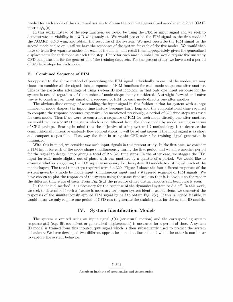
needed for each mode of the structural system to obtain the complete generalized aerodynamic force (GAF)matrix Qij(κ).

In this work, instead of the step function, we would be using the FIM as input signal and we seek todemonstrate its viability in a 3-D wing analysis. We would prescribe the FIM signal to the first mode ofthe AGARD 445.6 wing and obtain the response of the system. We next prescribe the FIM signal to thesecond mode and so on, until we have the responses of the system for each of the five modes. We would thenhave to train five separate models for each of the mode, and recall them appropriately given the generalizeddisplacements for each mode at each time step. Hence for each mach number, we would require five unsteadyCFD computations for the generation of the training data sets. For the present study, we have used a periodof 320 time steps for each mode.

B. Combined Sequence of FIM

As opposed to the above method of prescribing the FIM signal individually to each of the modes, we maychoose to combine all the signals into a sequence of FIM functions for each mode shape one after another.This is the particular advantage of using system ID methodology, in that only one input response for thesystem is needed regardless of the number of mode shapes being considered. A straight-forward and naıveway is to construct an input signal of a sequence of FIM for each mode directly one after another.

The obvious disadvantage of assembling the input signal in this fashion is that for system with a largenumber of mode shapes, the input time history becomes fairly long and the computational time requiredto compute the response becomes expensive. As mentioned previously, a period of 320 time steps was usedfor each mode. Thus if we were to construct a sequence of FIM for each mode directly one after another,we would require 5 × 320 time steps which is no different from the above mode by mode training in termsof CPU savings. Bearing in mind that the objective of using system ID methodology is to decrease thecomputationally intensive unsteady flow computations, it will be advantageous if the input signal is as shortand compact as possible. That way the time in using the CFD solver for training signal generation isminimized.

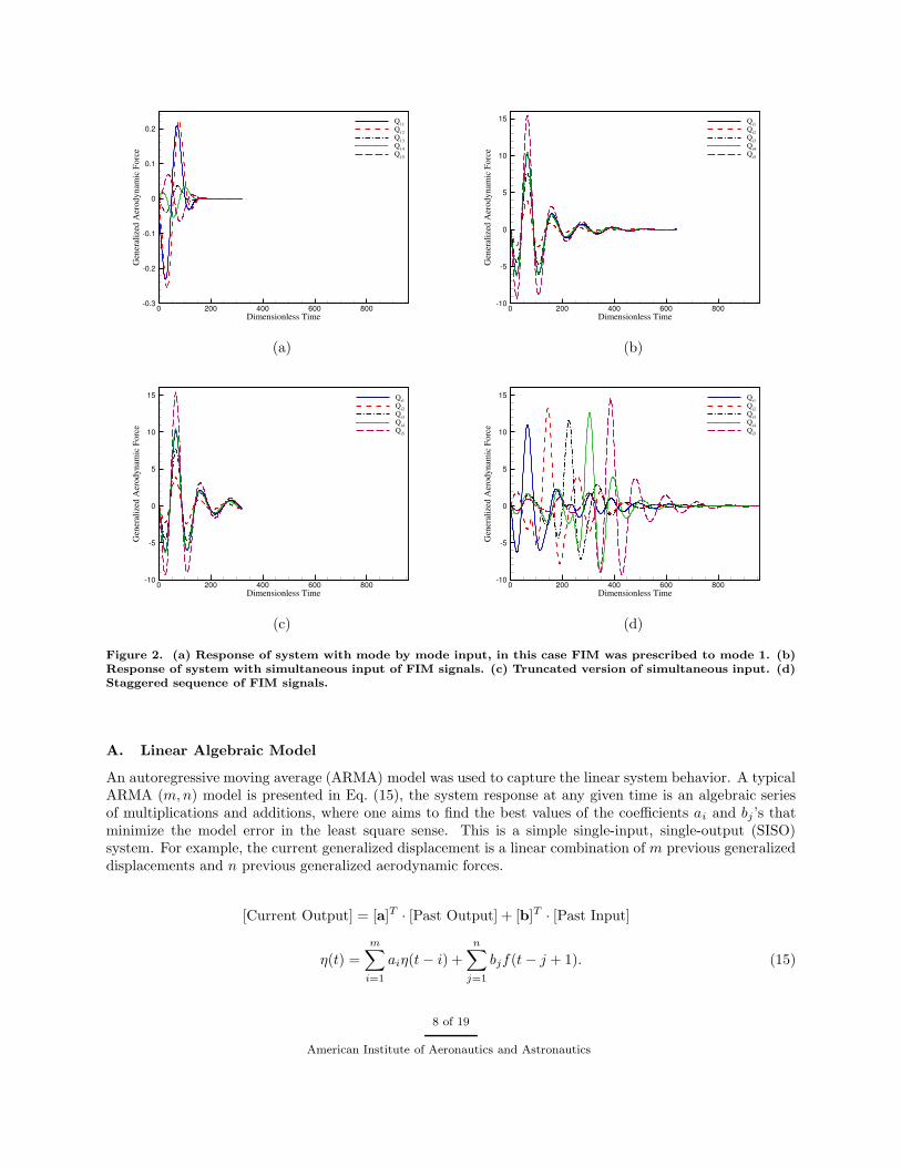
With this in mind, we consider two such input signals in this present study. In the first case, we considera FIM input for each of the mode shape simultaneously during the first period and we allow another periodfor the signal to decay, hence giving a total of 2 × 320 time steps. In the other case, we stagger the FIMinput for each mode slightly out of phase with one another, by a quarter of a period. We would like toexamine whether staggering the FIM input is necessary for the system ID models to distinguish each of themode shapes. The total time steps required were 3× 320. Figure 2 shows the four different responses of thesystem given by a mode by mode input, simultaneous input, and a staggered sequence of FIM signals. Wehave chosen to plot the responses of the system using the same time scale so that it is obvious to the readerthe different time steps of each. From Fig. 2(d) the presence of five distinct modes can been clearly seen.

In the indicial method, it is necessary for the response of the dynamical system to die off. In this work,we seek to determine if such a feature is necessary for proper system identification. Hence we truncated theresponses of the simultaneously applied FIM signal by half to obtain Fig. 2(c). If this is indeed feasible, itwould mean we only require one period of CFD run to generate the training data for the system ID models.

IV. System Identification Models

The system is excited using an input signal f(t) (structural motion) and the corresponding systemresponse η(t) (e.g. lift coefficient or generalized displacement) is measured for a period of time. A systemID model is trained from this input-output signal which is then subsequently used to predict the systembehaviour. We have developed two different approaches; one is a linear model while the other is non-linearto capture the system behavior.

7 of 19


Dimensionless Time

Gen

eral

ized

Aer

odyn

amic

Forc

e

0 200 400 600 800-0.3

-0.2

-0.1

0

0.1

0.2Q11Q12Q13Q14Q15

Dimensionless Time

Gen

eral

ized

Aer

odyn

amic

Forc

e

0 200 400 600 800-10

-5

0

5

10

15 Qi1Qi2Qi3Qi4Qi5

(a) (b)

Dimensionless Time

Gen

eral

ized

Aer

odyn

amic

Forc

e

0 200 400 600 800-10

-5

0

5

10

15 Qi1Qi2Qi3Qi4Qi5

Dimensionless Time

Gen

eral

ized

Aer

odyn

amic

Forc

e

0 200 400 600 800-10

-5

0

5

10

15 Qi1Qi2Qi3Qi4Qi5

(c) (d)

Figure 2. (a) Response of system with mode by mode input, in this case FIM was prescribed to mode 1. (b)Response of system with simultaneous input of FIM signals. (c) Truncated version of simultaneous input. (d)Staggered sequence of FIM signals.

A. Linear Algebraic Model

An autoregressive moving average (ARMA) model was used to capture the linear system behavior. A typicalARMA (m,n) model is presented in Eq. (15), the system response at any given time is an algebraic seriesof multiplications and additions, where one aims to find the best values of the coefficients ai and bj ’s thatminimize the model error in the least square sense. This is a simple single-input, single-output (SISO)system. For example, the current generalized displacement is a linear combination of m previous generalizeddisplacements and n previous generalized aerodynamic forces.

[Current Output] = [a]T · [Past Output] + [b]T · [Past Input]

η(t) =m

∑

i=1

aiη(t− i) +n

∑

j=1

bjf(t− j + 1). (15)

8 of 19


The optimal/best order of the model could be identified via numerical studies or design of experiments.Different combinations of the order is searched such that the error between the CFD time history and theprediction time history by the model is minimized. However there are certain caveats that the user has tobe aware of, firstly, the order of the past outputs, i.e. m should be at least 3. This is to account for thekinematics dimensionality of displacement, velocity and acceleration. Secondly, m would usually be less thanor equal to n. This is because higher orders of m capture only the wake effect which has only secondaryinfluence on the flow. The reader is referred to Ref. 18 for a more in-depth discussion.

In this paper, the coefficients of the linear algebraic model were obtained using a least square minimizationof error via Marquardt Levenberg algorithm. We employed a random multistart to minimize the chances ofgetting stuck at the local minima of the error function.

B. Non-linear Neural Network Model

It is fairly common to encounter instances where a linear model is not capable of capturing the systembehavior. In order to deal with such situations, we consider an artificial neural network model in placeof the linear algebraic model presented in Eq. (15). Artificial neural networks (ANN) have the ability toapproximate functions involving highly non-linear and complex data. Among the plethora of ANN paradigms,the Multilayer Perceptron (MLP) and Radial Basis Functions (RBF) are the most widely used networks.For the purpose of this paper, the RBF network was employed. RBF is classified as a supervised learningnetwork, in which there must exists a set of explicit targets for the network to match. Incorporating thesimilar concept of model order (m,n) as that of the ARMA model, we would set up the training data as a setof obervations of m previous generalized displacements and n previous generalized aerodynamic forces perobservation, we then train the RBF to “learn” the mapping between the inputs and the desired output forsuch an order. RBF networks have another added advantage in that they have been proven to be universalfunction approximators.27, 28

A radial basis function, φ, is one whose output is symmetric around an associated center, µ. That is:φ(x) = φ

(

‖x − µ‖)

, where the argument of φ is a chosen vector norm.29 Usually the Euclidean norm is

adopted30 and by selecting φ(r) = e−r2/σ2

, we would obtain the Gaussian function as an RBF, where σis the width or scale parameter. A set of RBFs can then serve as a basis for representing a wide class offunctions that are expressible as linear combinations of the chosen RBFs:

η(x) =

d∑

j=1

wjφ(

‖x− µj‖)

. (16)

Here d refers to the number of data points or training data and usually an RBF of this nature is veryexpensive to implement for large data set. Furthermore, it would not possess desirable prediction ability dueto over-fitting. Hence a generalized RBF network is usually preferred30, 31 as given by Eq. (17).

η(x) =

k∑

j=1

wjφ(

‖x− µj‖)

. (17)

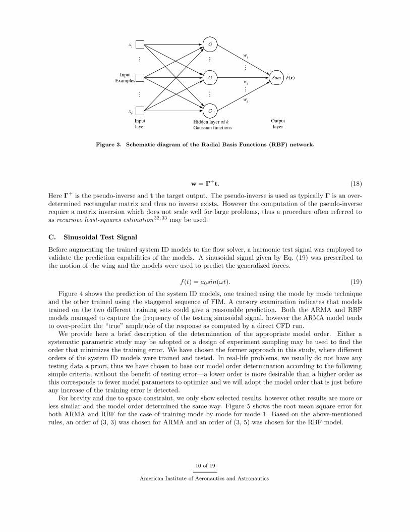
A typical structure of an RBF is presented in Fig. 3. As evident from the figure, an RBF network isnothing but a topological representation of Eq. (17) as a feed-forward network with three layers: the inputs,the hidden/kernel layer, and the output neuron(s). Each hidden neuron represents a single RBF with anassociated center position and width. Each output neuron performs a weighted summation of the hiddenneurons’ responses.

In Eq. (17), k is ordinarily smaller than d and wj ’s are the unknown sypnatic weight parameters thathave to be learned. It is further noted that µj ’s are found by a clustering algorithm and in this study, thecommonly used k-means clustering algorithm was employed. The learning of the RBF network is usuallyachieved through the pseudo-inverse solution, which gives a least square result:

9 of 19


G

G

G

w 1

w j

w k

F ( x )

x 1

Input Examples

x p

Input layer

Output layer

Sum

. .

.

. .

.

. .

.

. .

. . . .

. .

.

Hidden layer of Gaussian functions

k

Figure 3. Schematic diagram of the Radial Basis Functions (RBF) network.

w = Γ+t. (18)

Here Γ+ is the pseudo-inverse and t the target output. The pseudo-inverse is used as typically Γ is an over-determined rectangular matrix and thus no inverse exists. However the computation of the pseudo-inverserequire a matrix inversion which does not scale well for large problems, thus a procedure often referred toas recursive least-squares estimation32, 33 may be used.

C. Sinusoidal Test Signal

Before augmenting the trained system ID models to the flow solver, a harmonic test signal was employed tovalidate the prediction capabilities of the models. A sinusoidal signal given by Eq. (19) was prescribed tothe motion of the wing and the models were used to predict the generalized forces.

f(t) = a0sin(ωt). (19)

Figure 4 shows the prediction of the system ID models, one trained using the mode by mode techniqueand the other trained using the staggered sequence of FIM. A cursory examination indicates that modelstrained on the two different training sets could give a reasonable prediction. Both the ARMA and RBFmodels managed to capture the frequency of the testing sinusoidal signal, however the ARMA model tendsto over-predict the “true” amplitude of the response as computed by a direct CFD run.

We provide here a brief description of the determination of the appropriate model order. Either asystematic parametric study may be adopted or a design of experiment sampling may be used to find theorder that minimizes the training error. We have chosen the former approach in this study, where differentorders of the system ID models were trained and tested. In real-life problems, we usually do not have anytesting data a priori, thus we have chosen to base our model order determination according to the followingsimple criteria, without the benefit of testing error—a lower order is more desirable than a higher order asthis corresponds to fewer model parameters to optimize and we will adopt the model order that is just beforeany increase of the training error is detected.

For brevity and due to space constraint, we only show selected results, however other results are more orless similar and the model order determined the same way. Figure 5 shows the root mean square error forboth ARMA and RBF for the case of training mode by mode for mode 1. Based on the above-mentionedrules, an order of (3, 3) was chosen for ARMA and an order of (3, 5) was chosen for the RBF model.

10 of 19


50 100 150 200 250 300−1

−0.5

0

0.5

1

Dimensionless Time

Gen

eral

ized

Aero

dyna

mic

Forc

e, Q

11

CFDARMARBF

50 100 150 200 250 300

−1

−0.5

0

0.5

1

1.5

Dimensionless Time

Gen

eral

ized

Aero

dyna

mic

Forc

e, Q

22

CFDARMARBF

(a) (b)

Figure 4. (a) Prediction of Q11 via training of mode by mode. (b) Prediction of Q22 via training of combinedsignal.

1 2 3 4 5 6 7 8 90

0.05

0.1

0.15

0.2

0.25

0.3

03−0303−04

03−0504−04

04−0504−06

05−0505−06

06−06

RMS

Erro

r

Train ErrorTest Error

1 2 3 4 5 6 7 8 90

0.1

0.2

0.3

0.4

0.5

03−0303−04

03−0504−04

04−0504−06

05−0505−06

06−06

RMS

Erro

r

Train ErrorTest Error

(a) ARMA Model (b) RBF Model

Figure 5. Root mean square error of ARMA and RBF models for mode by mode training for mode 1.

V. AGARD 445.6 Wing

The AGARD 445.6 wing has a quarter-chord sweep angle of 45 degrees and its cross-section is given bythe NACA65a004 airfoil. The flutter characteristics of this wing were investigated experimentally over a widerange of Mach numbers.34 The results were presented as an AGARD standard aeroelastic configuration35

and have since been widely used to test and validate flutter calculations.In this section, the integrated system ID-CSD model is used to predict the flutter boundary for the

three-dimensional AGARD 455.6 wing. We consider the weakened wing model as listed in Ref. 34. Thewing is modeled by the first five natural vibrational modes, the first four modes are shown in Fig. 6. Theseare identified as the first bending, first torsion, second bending, and second torsion modes respectively. Thenatural frequencies of these modes are also shown in Fig. 6. Although the AGARD 445.6 wing is a multi-modal system, the first mode is the dominant mode and also usually the flutter mode, at least in the subsonicand transonic regimes.

11 of 19


Mode 1, f1 = 9.60Hz Mode 2, f2 = 38.17Hz

Mode 3, f3 = 48.35Hz Mode 4, f4 = 91.54Hz

Figure 6. Modal shape deflections and frequencies for the 445.6 wing (weakened model). Only alternate meshlines have been shown.

A. Model Evaluation

Before committing ourselves to determining the flutter boundary and Qij ’s using the integrated system ID-CSD model, we would like to first seek out the best system ID models to use. Figure 7 show the predictionsof both the ARMA and RBF models that have been trained on the responses of the simultaneous FIM inputand the truncated version.

Dimensionless Time

Gen

eral

ized

Disp

lace

men

t,M

ode1

0 100 200 300 400 500-0.004

-0.002

0

0.002

0.004

CFDSimult. Short ARMASimult. Long ARMASimult. Short RBFSimult. Long RBF

Dimensionless Time

Gen

eral

ized

Disp

lace

men

t,M

ode1

0 100 200 300

-1

-0.5

0

0.5

1CFDSimult. Short ARMASimult. Long ARMASimult. Short RBFSimult. Long RBF

(a) (b)

Figure 7. (a) Time history of the generalized coordinates for the AGARD 445.6 wing for M∞ = 0.96 andVf = 0.2, by ARMA and RBF trained on simultaneous FIM inputs. (b) M∞ = 1.141 and Vf = 0.75.

Evidently, the predictions of both the models are not too good. The ARMA model seems to eitheroverpredict or underpredict the amplitude of the true generalized displacement. And the RBF model seems

12 of 19


too erratic, this is especially highlighted in the “chattering” effect of the RBF prediction for M∞ = 0.96shown in figure 7(a). “Chattering” indicates a instability in the model and usually manifests itself withpredictions that oscillate back and forth randomly from the correct solution.18 This usually happens whentoo large a model order has been used and the model output is essentially over-correcting itself. In our casea low-order of (3, 4) was used, hence this might not be the true reason.

A possible explanation would be that too large a magnitude has been used in the simultaneous excitationof all the modes using FIM, hence allowing for large non-linearity to creep in. Future work might focus ondetermining the correct magnitude of FIM input signal to apply. This is so because the RBF model which isnon-linear in formulation seems to perform slightly better than the ARMA model, however secondary peaksseem to be present in the prediction of the RBF. Another point to note is that from our simulations, it seemsthat there is no significant difference in terms of prediction capabilities between the models trained on a longversion response of the simultaneous input and its truncated version.

We next show the results for the same scenarios via using the responses of mode by mode and staggeredsequence of FIM as the training data. From Fig. 8 it can be clearly seen that the predictions of themodels have improved. This is especially so for the ARMA model in the case of M∞ = 1.141, where theamplitudes are now correctly predicted. An implication of this is that a staggered sequence of FIM inputsis most probably necessary for the system ID models to properly distinguish between the different modesof the dynamical system. The results for the ARMA staggered model are not shown here as they were notsatisfactory. Thus for the rest of this paper, we would be presenting the results of ARMA and RBF trainedon mode by mode and RBF trained on staggered response.

Dimensionless Time

Gen

eral

ized

Disp

lace

men

t,M

ode1

0 100 200 300 400 500-0.004

-0.003

-0.002

-0.001

0

0.001

0.002

0.003

0.004CFDMode by Mode ARMAMode by Mode RBFStaggered RBF

Dimensionless Time

Gen

eral

ized

Disp

lace

men

t,M

ode1

0 100 200 300

-1

-0.5

0

0.5

1CFDMode by Mode ARMAMode by Mode RBFStaggered RBF

(a) (b)

Figure 8. (a) Time history of the generalized coordinates for the AGARD 445.6 wing for M∞ = 0.96 andVf = 0.2, by ARMA and RBF trained on mode by mode and staggered FIM inputs. (b) M∞ = 1.141 andVf = 0.75.

B. Generalized Aerodynamic Force

When an input signal f(t) is fed into a dynamical system, the frequency response of the system can then becalculated as:

A =F

(

η(t))

F(

f(t)) (20)

where η is the response of the system and F(·) is the Fourier transform of the signal. Figure 9 showsthe computation of the generalized aerodynamic forces Qij obtained using the results of the actual CFD

13 of 19


simulations. Another advantage of the system ID model is its ability to provide the GAF besides its fluttertime history prediction capability. To obtain the prediction of Qij for the staggered RBF model, we wouldfirstly train the model on the staggered response. Subsequently to obtain say, Q11, we prescribe a FIM inputto the first mode of the system ID-CSD model and record its subsequent response.

We will show that the use of a smooth FIM function which avoids the discontinuous nature of the stepfunction used by Ref. 2 is able to achieve the same results, we also show in the same figure that both ARMAand RBF models were able to provide reasonably accurate computations of the Qij ’s.

Reduced Frequency, κ

Gen

eral

ized

Aer

odyn

amic

Forc

e,Q

11

0 0.2 0.4 0.6 0.8 1-7

-6

-5

-4

-3

-2

-1

0CFDSimult. Long ARMASimult. Long RBF


Gen

eral

ized

Aer

odyn

amic

Forc

e,Q

12

0 0.2 0.4 0.6 0.8 1-50

-40

-30

-20

-10

0

10

20

CFDSimult. Long ARMASimult. Long RBF


Gen

eral

ized

Aer

odyn

amic

Forc

e,Q

21

0 0.2 0.4 0.6 0.8 1

0

1

2

CFDSimult. Long ARMASimult. Long RBF


Gen

eral

ized

Aer

odyn

amic

Forc

e,Q

22

0 0.2 0.4 0.6 0.8 1-20

-15

-10

-5

0

5

10CFDSimult. Long ARMASimult. Long RBF

Figure 9. Generalized aerodynamic force Q11, Q12, Q21, and Q22 for M∞ = 0.960. Models trained via simulta-neous input of FIM. 2 denotes real part, 4 denotes imaginary part.

Figure 9 shows the computed generalized aerodynamic forces Q11, Q12, Q21, and Q22 by the CFD andsystem ID methods respectively, for the first two vibrational modes. The models have been trained via thesimultaneuous input of FIM. From Fig. 9 it is noted that the predicted Qij for the models were inaccurateeven for the low reduced frequency, especially for the ARMA model. Whereas the models trained by themode by mode response and staggered sequence of input gave results that agreed quite well with that of theactual CFD computation, except for the high reduced frequency end, as shown in Fig. 10.

14 of 19



Gen

eral

ized

Aer

odyn

amic

Forc

e,Q

11

0 0.2 0.4 0.6 0.8 1-7

-6

-5

-4

-3

-2

-1



Gen

eral

ized

Aer

odyn

amic

Forc

e,Q

12

0 0.2 0.4 0.6 0.8 1-50

-40

-30

-20

-10

0

10

20

CFDMode by Mode ARMAMode by Mode RBFStaggered RBF


Gen

eral

ized

Aer

odyn

amic

Forc

e,Q

21

0 0.2 0.4 0.6 0.8 1-0.5

0

0.5

1

1.5

2

CFDMode by Mode ARMAMode by Mode RBFStaggered RBF


Gen

eral

ized

Aer

odyn

amic

Forc

e,Q

22

0 0.2 0.4 0.6 0.8 1-20

-15

-10

-5

0

5


Figure 10. Generalized aerodynamic force Q11, Q12, Q21, and Q22 for M∞ = 0.960. Models trained via mode bymode and staggered input of FIM. 2 denotes real part, 4 denotes imaginary part.

C. Flutter Time History

In this section we present the results of using the above identified three models for flutter predictions.Traditionally, for a particular Mach number regime, to determine the flutter point, the upper bound of thespeed index which exhibits instability and the lower bound of the speed index which exhibits stability aresought. A new CFD run is then computed at the mean value of the upper and lower bound to determinethe nature at this new speed index. Obviously, this is a computationally expensive procedure as every newspeed index has to be recomputed. With the system ID-CSD framework in place, we are now in a positionto determine the flutter boundary of the AGARD 445.6 wing via the bi-section method very much faster, asthe system ID models trained at a particular mach number would be able to predict the time histories forvarious speed index.

Figure 11(a) shows the flight condition M∞ = 0.96 and Vf = 0.25, as can be seen the predictions of thesystem ID models are quite accurate and they are able to predict the flutter boundary, which in this case isvery close to the neutral point. Although mode 1 is usually the dominant mode and modes 4 and 5 tend todamp out in time, we show in Fig. 11(b) the prediction of the models for mode 3, which is the second bending.In this case, the ARMA model exhibit a slight deterioration but nonetheless the stable and unstable trendshave been properly predicted which is more important. Finally figures 11(c) and 11(d) show the conditions

15 of 19


of flutter instability at flight conditions, M∞ = 0.85, Vf = 0.50, and M∞ = 0.678, Vf = 0.42, respectively.Although the RBF model was sufficiently accurate, the ARMA tends to overpredict the amplitudes near thestart.

Dimensionless Time

Gen

eral

ized

Disp

lace

men

t,M

ode1

0 100 200 300 400 500

-0.003

-0.002

-0.001

0

0.001

0.002

0.003

0.004


Dimensionless Time

Gen

eral

ized

Disp

lace

men

t,M

ode3

0 100 200 300 400 500

-0.0006

-0.0004

-0.0002

0

0.0002

0.0004


(a) (b)

Dimensionless Time

Gen

eral

ized

Disp

lace

men

t,M

ode1

0 100 200 300-0.4

-0.2

0

0.2


Dimensionless Time

Gen

eral

ized

Disp

lace

men

t,M

ode1

0 100 200 300 400-0.006

-0.005

-0.004

-0.003

-0.002

-0.001

0

0.001

0.002

0.003

0.004

0.005

0.006

0.007 CFDMode by Mode ARMAMode by Mode RBFStaggered RBF

(c) (d)

Figure 11. (a) Time history of the generalized coordinates for the AGARD 445.6 wing for M∞ = 0.96, Vf = 0.25,mode 1, by ARMA and RBF trained on mode by mode and staggered FIM inputs. (b) M∞ = 0.85, Vf = 0.30,mode 3. (c) M∞ = 0.85, Vf = 0.50, mode 1. (d) M∞ = 0.678, Vf = 0.42, mode 1.

Figure 12 shows the flutter boundary obtained using the RBF model trained on staggered FIM input.Although we have only considered five points in this paper, the results do demonstrate the efficacy of themethod as we could obtain a flutter boundary very close to the results of Liu et al.5

VI. Concluding Remarks

To aid the user in choosing the appropriate model and training data, the capabilities of each of thesystem ID models are summarized in table 1. The category—length of training data, refers to the number ofCFD runs needed to produce the training data for the models. Since both ARMA and RBF trained on themode by mode response require five CFD runs, they are given a low score. On the other hand, a staggered

16 of 19


Mach Number

Flut

terS

peed

Inde

x

0.3 0.4 0.5 0.6 0.7 0.8 0.9 1 1.1 1.2 1.3 1.40.2

0.3

0.4

0.5

0.6

0.7

0.8Liu et al., 2001ExperimentalStaggered RBF

Mach Number

Flut

terF

requ

ency

Ratio

0.3 0.4 0.5 0.6 0.7 0.8 0.9 1 1.1 1.2 1.3 1.40.2

0.3

0.4

0.5

0.6

0.7

0.8Liu et al., 2001ExperimentalStaggered RBF

(a) (b)

Figure 12. (a) Flutter speed for the AGARD 445.6 wing. (b) Flutter frequency for the AGARD 445.6 wing.

sequence of FIM input requires three periods which is equivalent to three CFD runs, hence it was awardedslightly higher. As for ease of implementation, both types of models require a fair bit of domain knowledgeeach, hence this was judged to be equal.

The next criteria was accuracy. Although the accuracy of the model is highly dependent on the typeof training data, generally the ARMA model is the least accurate as it tends to give overprediction butthe trend of the time history is predicted. As for the two RBF models, the one trained on the staggeredsequence of FIM was found to be the most accurate. Robustness refers to the ability of the system ID modelsto provide both the time history and also the generalized aerodynamic force, Qij (to be discussed later) withthe same trained model. In this aspect, the RBF model being non-linear by formulation is able provide botha more accurate time history and Qij plots as compared to the ARMA model.

Table 1. Comparison between system ID models and forms of training.

Length of Training Data Ease of Implementation Accuracy Robustness

Mode by Mode ARMA√ √√ √ √

Mode by Mode RBF√ √√ √√ √√

Staggered RBF√√ √√ √√√ √√

To conclude, the following could be drawn from the results of this paper:

• For flutter computations, the system ID models trained on data of mode by mode and staggeredsequence of FIM are capable of predicting the general trend of responses at different reduced frequencies.

• The ARMA model seems to work fairly well in the case of mode by mode training where the modes aredecoupled and linearized, whereas RBF is able to handle both a mode by mode case and a staggeredsequence of FIM. With the latter resulting in more CPU savings as it requires less time to create thetraining data.

• It would seem that truncating the training data without a need for decay would provide adequate“information” for the system ID models.

17 of 19


• The advantage of employing system ID models over the indicial method is that besides being capableof providing the Qij ’s, the system ID models are also capable of giving the complete time history ofthe generalized displacements for a dynamical system.

• Further investigation is necessary to understand the effects of the magnitude of input signals in the caseof simultaneuous FIM input, as our results suggest large non-linearity effects in the system responsecausing a breakdown of the system ID models.

References

1Won, K. S., Tsai, H. M., Ray, T., and Liu, F., “Flutter Simulation and Prediction via Identification of Non-linear ImpulseResponse,” 43rd AIAA Aerospace Sciences Meeting and Exhibit, AIAA Paper 2005-0834, Jan. 10–13, Reno, NV, 2005.

2Ballhaus, W. F. and Goorjian, P. M., “Computation of Unsteady Transonic Flows by the Indicial Method,” AIAA

Journal, Vol. 16, No. 2, 1978, pp. 117–124.3Sadeghi, M., Yang, S., Liu, F., and Tsai, H. M., “Parallel Computation of Wing Flutter with a Coupled Navier-

Stokes/CSD Method,” 41st AIAA Aerospace Sciences Meeting and Exhibit, AIAA Paper 2003-1347, Jan. 6–9, Reno, NV,2003.

4Tsai, H. M., Wong, A. S. F., Cai, J., Zhu, Y., and Liu, F., “Unsteady Flow Calculations with a Multi-Block MovingMesh Algorithm,” AIAA Journal, Vol. 39, No. 6, 2001, pp. 1021–1029.

5Liu, F., Cai, J., Zhu, Y., Tsai, H. M., and Wong, A. S. F., “Calculation of Wing Flutter by a Coupled Fluid-StructureMethod,” Journal of Aircraft, Vol. 38, 2001, pp. 334–342.

6Pember, R. B., Bell, J. B., and Collela, P., “An Adaptive Cartesian Grid Method for Unsteady Compressible Flow inIrregular Regions,” Journal of Computational Physics, Vol. 120, 1995, pp. 278–304.

7Melton, J. E., Berger, M. J., Aftosmis, M. J., and Wong, M. D., “3D Applications of A Cartesian Grid Euler Method,”AIAA Paper 1995-0853, 1995.

8Forrer, H. and Jeltsch, R., “A Higher Order Boundary Treatment for Cartesian-Grid Methods,” Journal of Computational

Physics, Vol. 140, 1998, pp. 259–277.9Lahur, P. R. and Nakamura, Y., “Simulation of Flow around Moving 3D Body on Unstructured Cartesian Grid.” AIAA

Paper 2001-2605, June 2001.10Murman, S. M., Aftosmis, M. J., and Berger, M. J., “Implicit Approaches for Moving Boundaries in a 3-D Cartesian

Method.” 41st AIAA Aerospace Sciences Meeting and Exhibit, AIAA Paper 2003-1119, Jan. 6–9, Reno, NV, 2003.11Yang, S., Liu, F., Luo, S., Tsai, H. M., and Schuster, D. M., “Time-Domain Aeroelastic Simulation on Stationary Body-

Conforming Grids with Small Perturbation Boundary Conditions,” 42nd AIAA Aerospace Sciences Meeting and Exhibit, AIAAPaper 2004-0885, Jan. 5–8, Reno, NV, 2004.

12Sankar, L., Malone, J., and Tassa, Y., “An Implicit Conservative Algorithm for Steady and Unsteady Three-DimensionalTransonic Potential Flows,” AIAA Paper 1981-1016, June 1981.

13Sankar, L., Malone, J., and Schuster, D., “Euler Solutions for Transonic Flow Past a Fighter Wing,” Journal of Aircraft,Vol. 24, No. 1, Jan. 1987, pp. 10–16.

14Fisher, C. C. and Arena, A. S., “Calculation of Airfoil Flutter by an Euler Method with Approximate Boundary Condi-tions,” AIAA Paper 2003-3830, June 2003.

15Ljung, L., “System Identification: Theory for the User,” Prentice Hall, Inc., New Jersey, 1997.16Silva, W. A., “Application of Non-linear Systems Theory to Transonic Unsteady Aerodynamic Responses,” Journal of

Aircraft, Vol. 30, No. 5, 1993, pp. 660–680.17Liu, F., Cai, J., and Tsai, H. M., “Flutter Predictions by a Filtered Impulse Method,” AIAA Paper 2000-4230, Aug.,

2000.18Cowan, T. J., Arena, A. S., and Gupta, K. K., “Accelerating Computational Fluid Dynamics Based Aeroelastic Predic-

tions Using System Identification,” Journal of Aircraft, Vol. 38, No. 1, Jan.-Feb., 2001.19Liu, F. and Zheng, X., “A Strongly-Coupled Time-Marching Method for Solving the Navier-Stokes and k-ω Turbulence

Model Equations with Multigrid,” Journal of Computational Physics, Vol. 128, 1996, pp. 289–300.20Liu, F. and Ji, S., “Unsteady Flow Calculations with a Multigrid Navier-Stokes Method,” AIAA Journal, Vol. 34, No.

10, Oct. 1996, pp. 2047–2053.21Jameson, A., Schmidt, W., and Turkel, E., “Numerical Solutions of the Euler Equations by Finite Volume Methods Using

Runge-Kutta Time-Stepping Schemes,” AIAA Paper 81-1259, 1981.22Lai, K. L., Tsai, H. M., and Lum, K. Y., “A CFD and CSD Interaction Algorithm for Large and Complex Configurations,”

AIAA Paper 2002-2715, 2002.23Sadeghi, M., Liu, F., Lai, K. L., and Tsai, H. M., “Application of Three-Dimensional Interfaces for Data Transfer in

Aeroelastic Computations,” AIAA Paper 2004-5376, 2004.24Seidel, D., Bennet, R., and Ricketts, R., “Some Recent Applications of XTRAN3S,” AIAA Paper 1983-1811, July, 1983.

18 of 19


25Hassig, H. J., “Approximate True Damping Solution of the Flutter Equation by Determinant Iteration,” Journal of

Aircraft, Vol. 8, No. 11, 1971, pp. 885–889.26Tobak, M., “On the Use of Indicial Function Concept in the Analysis of Unsteady Motions of Wings and Wing-Tail

Combinations,” NACA Rept. 1188, 1954.27Hornik, K., Stinchcombe, M., and White, H., “Multilayer Feedforward Networks are Universal Approximators,” Neural

Networks, Vol. 2, 1989, pp. 359–366.28Poggio, T. and Girosi, F., “Networks and the Best Approximation Property,” Biological Cybernetics, Vol. 63, 1989, pp.

169–176.29Sundararajan, N. and Saratchandran, P., “Radial Basis Function Neural Networks with Sequential Learning,” World

Scientific Publishing Co. Ltd., London, UK, 1999.30Jin, Y., “A Comprehensive Survey of Fitness Approximation in Evolutionary Computation,” Soft Computing, Springer-

Verlag, 2003.31Haykin, S., “Neural Networks: A Comprehensive Foundation,” 2nd Edition, Prentice Hall Internal Inc., New Jersey, 1999.32Astrom, K. and Wittenmark, B., “Computer Controlled Systems: Theory and Designs,” Englewood Cliffs, NJ, Prentice

Hall, 1984.33Strobach, P., “Linear Prediction Theory: A Mathematical Basis for Adaptive Systems,” New York, Springer-Verlag, 1990.34Yates, E. C., Land, N. S., and Foughner, J. T., “Measured and Calculated Subsonic and Transonic Flutter Characteristics

of a 45 ◦ Sweptback Wing Planform in Air and in Freon-12 in the Langley Transonic Dynamics Tunnel,” AGARD TN D-1616,1963.

35“AGARD Standard Aeroelastic Configurations for Dynamic Response I – Wing 445.6,” NASA TM 100492, Aug., 1987.

19 of 19


non-linear impulse methods for aeroelastic …fliu.eng.uci.edu/publications/c069.pdfnon-linear...

Documents