non-linear mixed effects modelling using the sas … 2004 uppsala 2 what this talk hopes to show......
TRANSCRIPT
Exprimo Consulting
Non-linear mixed effects modelling using the SAS system - An overview
17 June 2004Al Maloney

PAGE 2004 Uppsala 2
What this talk hopes to show...
Fitting non-linear mixed effect models in SAS using the NLMIXEDprocedure.
Background The syntax - defining the modelThe options - defining the criteria for fitting the modelStrengths and LimitationsSummary(If time, a very brief example using NLMIXED - adaptive design)
This outline is based on the SAS online documentation !
PAGE 2004 Uppsala 3
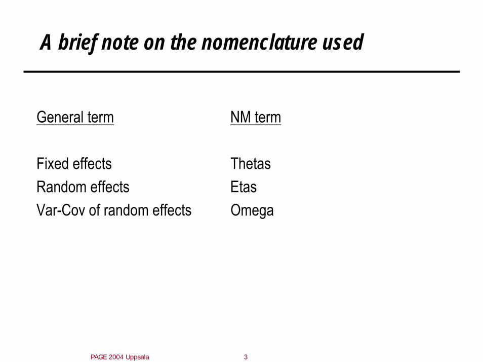
A brief note on the nomenclature used
General term NM term
Fixed effects ThetasRandom effects EtasVar-Cov of random effects Omega

PAGE 2004 Uppsala 4
SAS seem to have incorporated the current 'best' knowledge on NL mixed models methods
Built on work from a number of 'different' fields including:
Beal, Sheiner... Mixed models in PK / PK-PDGoldstein... Hierarchical mixed modelsLongford, Diggle... Generalised linear mixed modelsLindstrom, Bates, Pinheiro... General applied mixed models Davidian, Giltinan... Heteroscedastistic/NP mixed models
....+ SAS's own knowledge as well !
This has been 'packaged' in a new SAS procedure - PROC NLMIXED

PAGE 2004 Uppsala 5
PROC NLMIXED has a number of program statements which can be used
The following statements can be used with the NLMIXED procedure:
PROC NLMIXED options procedure call and options ARRAY array specification PARMS parameters and starting values BOUNDS boundary constraints BY variables CONTRAST 'label' expression ID expressions MODEL model specification RANDOM random effects specification PREDICT expression ESTIMATE 'label' expression ODS output controlREPLICATE replicate variable Program statements usual SAS programming statementsRun;

PAGE 2004 Uppsala 6
This talk will focus on the main statements
The most important statements are:
PROC NLMIXED options procedure call and options ARRAY array specification PARMS parameters and starting values BOUNDS boundary constraints BY variables CONTRAST 'label' expressionID expressions MODEL model specification RANDOM random effects specification PREDICT expression ESTIMATE 'label' expressionODS output controlREPLICATE replicate variable Program statements usual SAS programming statementsRun;

PAGE 2004 Uppsala 7
To help interpret the programming statements, consider some artificial data
Example results from 1 study of 10
9
10
11
12
13
14
0 2 4 6 8 10 12
Time (months)
Resp
onse
Placebo 50mg 100mg

PAGE 2004 Uppsala 8
To help interpret the programming statements, consider some artificial data
Example results from 1 study of 10
9
10
11
12
13
14
0 2 4 6 8 10 12
Time (months)
Res
pons
e
Placebo 50mg 100mg
disease progression
drug onset
dose maximum effect

PAGE 2004 Uppsala 9
The dataset to be used in the NLMIXED procedure has the relevant data
Data PAGE;...Input Study Drug Dose Time Observed...
1 A 50 0 10.01 A 50 1 10.9
....2 B 0 0 10.0
10 Studies (random effect level)3 Drugs ("A" "B" and "C")
PAGE 2004 Uppsala 10
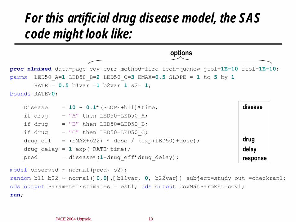
For this artificial drug disease model, the SAS code might look like:
proc nlmixed data=page cov corr method=firo tech=quanew gtol=1E-10 ftol=1E-10;parms LED50_A=1 LED50_B=2 LED50_C=3 EMAX=0.5 SLOPE = 1 to 5 by 1
RATE = 0.5 b1var =1 b2var 1 s2= 1;bounds RATE>0;
Disease = 10 + 0.1*(SLOPE+b11)*time;if drug = "A" then LED50=LED50_A;if drug = "B" then LED50=LED50_B;if drug = "C" then LED50=LED50_C;drug_eff = (EMAX+b22) * dose / (exp(LED50)+dose);drug_delay = 1-exp(-RATE*time);pred = disease*(1+drug_eff*drug_delay);
model observed ~ normal(pred, s2);random b11 b22 ~ normal([0,0],[b11var, 0, b22var]) subject=study out =checkran1; ods output ParameterEstimates = est1; ods output CovMatParmEst=cov1;run;
options
disease
drugdelayresponse
PAGE 2004 Uppsala 11
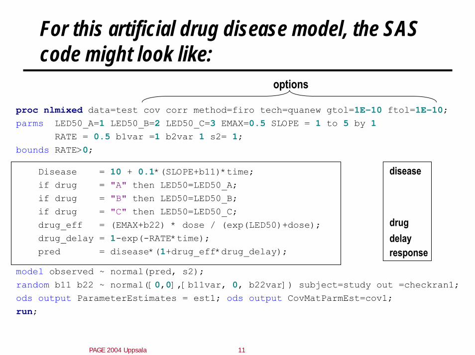
For this artificial drug disease model, the SAS code might look like:
proc nlmixed data=test cov corr method=firo tech=quanew gtol=1E-10 ftol=1E-10;parms LED50_A=1 LED50_B=2 LED50_C=3 EMAX=0.5 SLOPE = 1 to 5 by 1
RATE = 0.5 b1var =1 b2var 1 s2= 1;bounds RATE>0;
Disease = 10 + 0.1*(SLOPE+b11)*time;if drug = "A" then LED50=LED50_A;if drug = "B" then LED50=LED50_B;if drug = "C" then LED50=LED50_C;drug_eff = (EMAX+b22) * dose / (exp(LED50)+dose);drug_delay = 1-exp(-RATE*time);pred = disease*(1+drug_eff*drug_delay);
model observed ~ normal(pred, s2);random b11 b22 ~ normal([0,0],[b11var, 0, b22var]) subject=study out =checkran1; ods output ParameterEstimates = est1; ods output CovMatParmEst=cov1;run;
options
disease
drugdelayresponse

PAGE 2004 Uppsala 12
The "PARMS" statement defines starting points or initial grid search for each parameter
proc nlmixed data=test cov corr method=firo tech=quanew gtol=1E-10 ftol=1E-10;parms LED50_A=1 LED50_B=2 LED50_C=3 EMAX=0.5 SLOPE = 1 to 5 by 1
RATE = 0.5 b1var =1 b2var 1 s2= 1;bounds RATE>0;
Disease = 10 + 0.1*(SLOPE+b11)*time;if drug = "A" then LED50=LED50_A;if drug = "B" then LED50=LED50_B;if drug = "C" then LED50=LED50_C;drug_eff = (EMAX+b22) * dose / (exp(LED50)+dose);drug_delay = 1-exp(-RATE*time);pred = disease*(1+drug_eff*drug_delay);
model observed ~ normal(pred, s2);random b11 b22 ~ normal([0,0],[b11var, 0, b22var]) subject=study out =checkran1; ods output ParameterEstimates = est1; ods output CovMatParmEst=cov1;run;
disease
drugdelayresponse

PAGE 2004 Uppsala 13
The "PARMS" statement defines starting points or initial grid search for each parameter
The "PARMS" statement gives initial estimates for the model parameters. You can also give a range of potential values. SAS will perform the gridsearch, and start the optimisation at the best combination.
Example:
parms LED50_A=1 LED50_B=2 LED50_C=3 EMAX=0.5
slope = 1 to 5 by 1 b1var=1 b2var=1 s2= 1 RATE = 0.5;
Note the use of "TO" and "BY".Can use this to simply plot the likelihood function (no fitting). Can read in previous model fit parameters.

PAGE 2004 Uppsala 14
The "BOUNDS" and "BY" statements do exactly what you would expect.
proc nlmixed data=test cov corr method=firo tech=quanew gtol=1E-10 ftol=1E-10;parms LED50_A=1 LED50_B=2 LED50_C=3 EMAX=0.5 SLOPE = 1 to 5 by 1
RATE = 0.5 b1var =1 b2var 1 s2= 1;bounds RATE>0;
Disease = 10 + 0.1*(SLOPE+b11)*time;if drug = "A" then LED50=LED50_A;if drug = "B" then LED50=LED50_B;if drug = "C" then LED50=LED50_C;drug_eff = (EMAX+b22) * dose / (exp(LED50)+dose);drug_delay = 1-exp(-RATE*time);pred = disease*(1+drug_eff*drug_delay);
model observed ~ normal(pred, s2);random b11 b22 ~ normal([0,0],[b11var, 0, b22var]) subject=study out =checkran1; ods output ParameterEstimates = est1; ods output CovMatParmEst=cov1;run;
disease
drugdelayresponse

PAGE 2004 Uppsala 15
The "BOUNDS" and "BY" statements do exactly what you would expect.
The "BOUNDS" statement Limits on any parameters (although should generally be avoided with model reparameterisation and/or reduction).
Example: bounds RATE>0;
The "BY" statement
Useful for repeated model fitting (e.g. bootstrap samples)
Example :
by boot_sample;

PAGE 2004 Uppsala 16
The "MODEL" statement allows a wide variety of models, including defining your own log likelihood
proc nlmixed data=test cov corr method=firo tech=quanew gtol=1E-10 ftol=1E-10;parms LED50_A=1 LED50_B=2 LED50_C=3 EMAX=0.5 SLOPE = 1 to 5 by 1
RATE = 0.5 b1var =1 b2var 1 s2= 1;bounds RATE>0;
Disease = 10 + 0.1*(SLOPE+b11)*time;if drug = "A" then LED50=LED50_A;if drug = "B" then LED50=LED50_B;if drug = "C" then LED50=LED50_C;drug_eff = (EMAX+b22) * dose / (exp(LED50)+dose);drug_delay = 1-exp(-RATE*time);pred = disease*(1+drug_eff*drug_delay);
model observed ~ normal(pred, s2);random b11 b22 ~ normal([0,0],[b11var, 0, b22var]) subject=study out =checkran1; ods output ParameterEstimates = est1; ods output CovMatParmEst=cov1;run;
disease
drugdelayresponse

PAGE 2004 Uppsala 17
The "MODEL" statement allows a wide variety of models, including defining your own log likelihood
The "MODEL" statement defines the type of likelihood function.
Valid distributions are as follows.normal(m,v) specifies a normal distribution with mean m and variance v. binary(p) specifies a binary (Bernouilli) distribution with probability p. binomial(n,p) specifies a binomial distribution with count n and probability p. poisson(m) specifies a Poisson distribution with mean m. general(ll) specifies a general log likelihood function that you define.
Examples
model observed ~ normal(pred, s2);
ll=-.5*log(2*3.14159265358979*s2)-(.5/s2)*(y-pred)**2;
model y~general(ll);
or equivalently

PAGE 2004 Uppsala 18
The "RANDOM" statement defined the variance covariance matrix of random effects
proc nlmixed data=test cov corr method=firo tech=quanew gtol=1E-10 ftol=1E-10;parms LED50_A=1 LED50_B=2 LED50_C=3 EMAX=0.5 SLOPE = 1 to 5 by 1
RATE = 0.5 b1var =1 b2var 1 s2= 1;bounds RATE>0;
Disease = 10 + 0.1*(SLOPE+b11)*time;if drug = "A" then LED50=LED50_A;if drug = "B" then LED50=LED50_B;if drug = "C" then LED50=LED50_C;drug_eff = (EMAX+b22) * dose / (exp(LED50)+dose);drug_delay = 1-exp(-RATE*time);pred = disease*(1+drug_eff*drug_delay);
model observed ~ normal(pred, s2);random b11 b22 ~ normal([0,0],[b11var, 0, b22var]) subject=study out =checkran1; ods output ParameterEstimates = est1; ods output CovMatParmEst=cov1;run;
disease
drugdelayresponse

PAGE 2004 Uppsala 19
The "RANDOM" statement defined the variance covariance matrix of random effects
Define (lower) diagonal and off-diagonal random elements that need to be estimated.e.g. Simple two random effects, no correlation
Ω11 00 Ω22
random b11 b22 ~ normal([0,0],[b11var, 0, b22var]) subject=study out =checkran1;
e.g. Ω11 Ω12 Ω13 0Ω12 Ω22 Ω23 Ω24
Ω13 Ω23 Ω33 00 Ω24 0 Ω44
random b1 b2 b3 b4 ~ normal([0,0,0,0],[Ω11,Ω12,Ω22,Ω13,Ω23,Ω33,0,Ω24,0,Ω44]) subject=study;
PAGE 2004 Uppsala 20
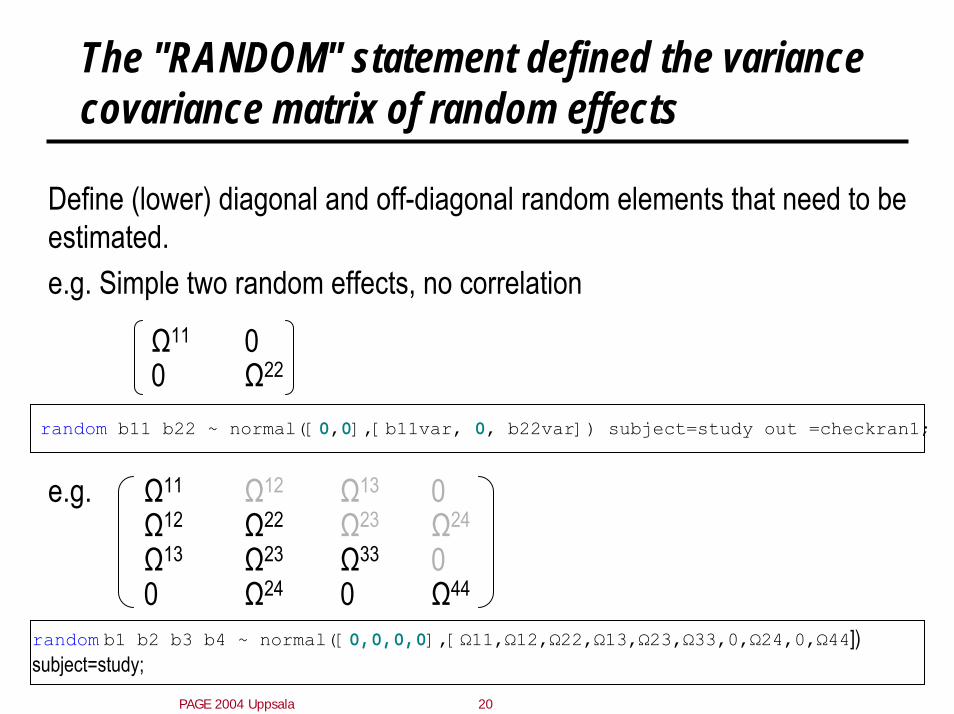
The "RANDOM" statement defined the variance covariance matrix of random effects
Define (lower) diagonal and off-diagonal random elements that need to be estimated.e.g. Simple two random effects, no correlation
Ω11 00 Ω22
random b11 b22 ~ normal([0,0],[b11var, 0, b22var]) subject=study out =checkran1;
e.g. Ω11 Ω12 Ω13 0Ω12 Ω22 Ω23 Ω24
Ω13 Ω23 Ω33 00 Ω24 0 Ω44
random b1 b2 b3 b4 ~ normal([0,0,0,0],[Ω11,Ω12,Ω22,Ω13,Ω23,Ω33,0,Ω24,0,Ω44]) subject=study;

PAGE 2004 Uppsala 21
The Output Deliver System (ODS) in SAS allows any output to be available later
proc nlmixed data=test cov corr method=firo tech=quanew gtol=1E-10 ftol=1E-10;parms LED50_A=1 LED50_B=2 LED50_C=3 EMAX=0.5 SLOPE = 1 to 5 by 1
RATE = 0.5 b1var =1 b2var 1 s2= 1;bounds RATE>0;
Disease = 10 + 0.1*(SLOPE+b11)*time;if drug = "A" then LED50=LED50_A;if drug = "B" then LED50=LED50_B;if drug = "C" then LED50=LED50_C;drug_eff = (EMAX+b22) * dose / (exp(LED50)+dose);drug_delay = 1-exp(-RATE*time);pred = disease*(1+drug_eff*drug_delay);
model observed ~ normal(pred, s2);random b11 b22 ~ normal([0,0],[b11var, 0, b22var]) subject=study out =checkran1; ods output ParameterEstimates = est1; ods output CovMatParmEst=cov1;run;
disease
drugdelayresponse

PAGE 2004 Uppsala 22
The Output Deliver System (ODS) in SAS allows any output to be available later
Any output that is can be written to the results file can also be saved to a dataset for subsequent manipulation. This includes:
Parameter estimatesFit statistics Model specificationCovariance matrixCorrelation matrixConvergence statusetc.
ods output ParameterEstimates = est1; ods output CovMatParmEst=cov1;
e.g.
PAGE 2004 Uppsala 23
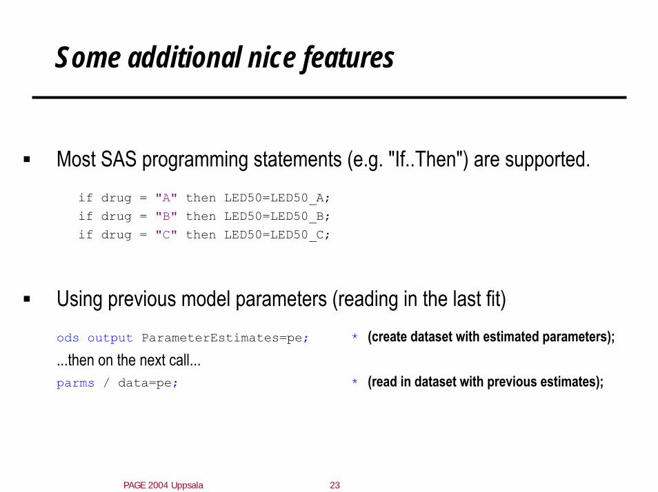
Some additional nice features
Most SAS programming statements (e.g. "If..Then") are supported.if drug = "A" then LED50=LED50_A;if drug = "B" then LED50=LED50_B;if drug = "C" then LED50=LED50_C;
Using previous model parameters (reading in the last fit)ods output ParameterEstimates=pe; * (create dataset with estimated parameters);...then on the next call... parms / data=pe; * (read in dataset with previous estimates);

PAGE 2004 Uppsala 24
Options in the model fitting
Where SAS shows it's strength, and the complexities of fitting these models !

PAGE 2004 Uppsala 25
Some of the main options are:
Basic OptionsDATA=input data setMETHOD=integration method
Optimisation SpecificationsTECHNIQUE=minimization techniqueUPDATE=update techniqueLINESEARCH=line-search methodLSPRECISION=line-search precisionHESCAL=type of Hessian scalingINHESSIAN=start for approximated HessianRESTART=iteration number for update restartOPTCHECK[=]check optimality in neighbourhood
Displayed Output Specifications
START=gradient at starting valuesHESS=Hessian matrixITDETAILS =iteration detailsCORR=correlation matrixCOV=covariance matrixECORR=corr matrix of additional estimatesECOV=cov matrix of additional estimatesEDER=derivatives of additional estimatesALPHA==alpha for confidence limitsDF=degrees of freedom for p values and
confidence limits
Termination Criteria SpecificationsMAXFUNC=maximum number of function callsMAXITER=maximum number of iterationsMINITER=minimum number of iterationsMAXTIME=upper limit seconds of CPU timeABSCONV=absolute function convergence criterionABSFCONV=absolute function convergence criterionABSGCONV=absolute gradient convergence criterionABSXCONV=absolute parameter convergence criterionFCONV=relative function convergence criterionFCONV2=relative function convergence criterionGCONV=relative gradient convergence criterionXCONV=relative parameter convergence criterionFDIGITS=number accurate digits in objective functionFSIZE=used in FCONV, GCONV criterionXSIZE=used in XCONV criterion
Derivatives SpecificationsFD[=]finite-difference derivativesFDHESSIAN[=]finite-difference second derivativesDIAHES=use only diagonal of Hessian
PAGE 2004 Uppsala 26
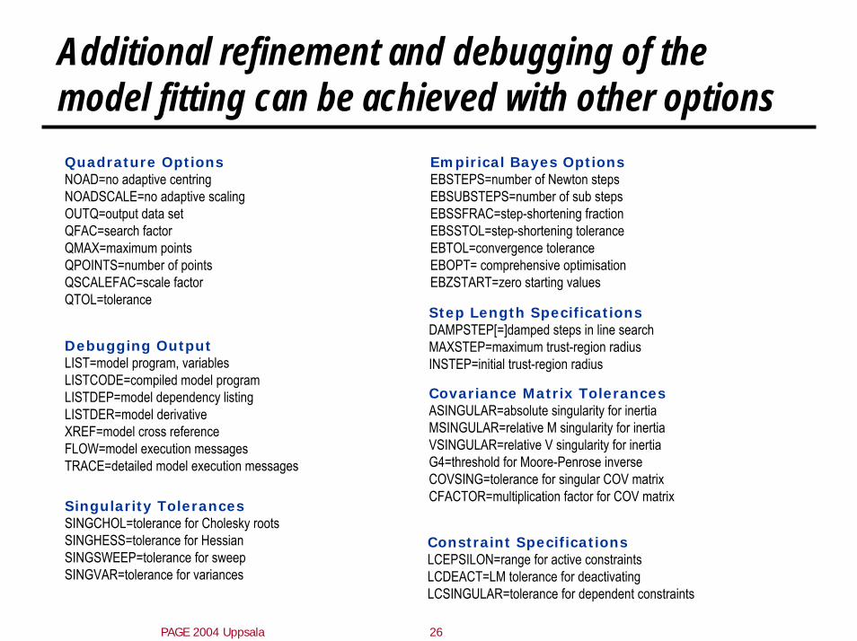
Additional refinement and debugging of the model fitting can be achieved with other optionsQuadrature OptionsNOAD=no adaptive centringNOADSCALE=no adaptive scalingOUTQ=output data setQFAC=search factorQMAX=maximum pointsQPOINTS=number of pointsQSCALEFAC=scale factorQTOL=tolerance
Empirical Bayes OptionsEBSTEPS=number of Newton stepsEBSUBSTEPS=number of sub stepsEBSSFRAC=step-shortening fractionEBSSTOL=step-shortening toleranceEBTOL=convergence toleranceEBOPT= comprehensive optimisationEBZSTART=zero starting values
Step Length SpecificationsDAMPSTEP[=]damped steps in line searchMAXSTEP=maximum trust-region radiusINSTEP=initial trust-region radius
Covariance Matrix TolerancesASINGULAR=absolute singularity for inertiaMSINGULAR=relative M singularity for inertiaVSINGULAR=relative V singularity for inertiaG4=threshold for Moore-Penrose inverseCOVSING=tolerance for singular COV matrixCFACTOR=multiplication factor for COV matrix
Debugging OutputLIST=model program, variablesLISTCODE=compiled model programLISTDEP=model dependency listingLISTDER=model derivativeXREF=model cross referenceFLOW=model execution messagesTRACE=detailed model execution messages
Singularity TolerancesSINGCHOL=tolerance for Cholesky rootsSINGHESS=tolerance for HessianSINGSWEEP=tolerance for sweepSINGVAR=tolerance for variances
Constraint SpecificationsLCEPSILON=range for active constraintsLCDEACT=LM tolerance for deactivatingLCSINGULAR=tolerance for dependent constraints
PAGE 2004 Uppsala 27
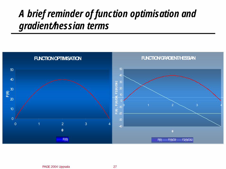
A brief reminder of function optimisation and gradient/hessian terms
FUNCTION OPTIMISATION
0
10
20
30
40
50
0 1 2 3 4
θ
F(θ)
F(θ)
FUNCTION/GRADIENT/HESSIAN
-40
-30
-20
-10
0
10
20
30
40
50
0 1 2 3 4
θ
F(θ)
, F(θ)
/Dθ,
F2(θ)
/Dθ2
F(θ) F(θ)/Dθ F2(θ)/Dθ2
PAGE 2004 Uppsala 28
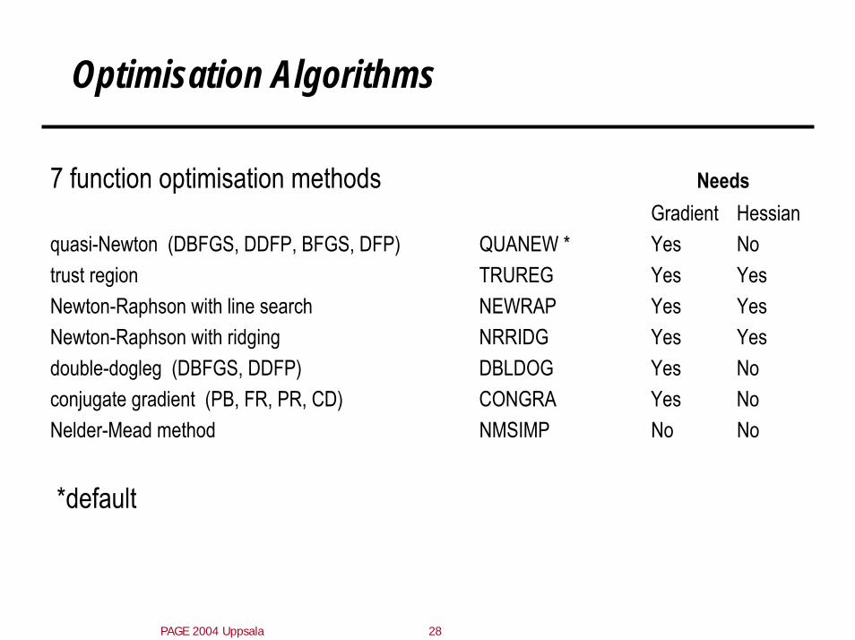
Optimisation Algorithms
7 function optimisation methods NeedsGradient Hessian
quasi-Newton (DBFGS, DDFP, BFGS, DFP) QUANEW * Yes Notrust region TRUREG Yes YesNewton-Raphson with line search NEWRAP Yes YesNewton-Raphson with ridging NRRIDG Yes Yesdouble-dogleg (DBFGS, DDFP) DBLDOG Yes Noconjugate gradient (PB, FR, PR, CD) CONGRA Yes NoNelder-Mead method NMSIMP No No
*default

PAGE 2004 Uppsala 29
Finite difference approximations of derivatives - forward or central?
SAS uses numerical approximations for derivatives.Gradient - first order derivatives - rate of change of functionHessian - second order derivatives - rate of change of rate of change
Consider the gradient:
Forward
Central

PAGE 2004 Uppsala 30
A quick reminder of forward and central numerical derivatives calculations
DF/Dθ = 0

PAGE 2004 Uppsala 31
Integral Approximations
First Order (as per NM)Taylors series expansion around ui=0 Only normal data
Adaptive gaussian quadrature (default)Centres integral at ui, the empirical bayes estimate Can choose number of quadrature points (1 = Laplacian approx.)
Likelihood

PAGE 2004 Uppsala 32
Termination Criteria - Convergence limits and diagnostics
Convergence is something you decide...not the computer package!
QUANEW algorithm will converge if any of the following are satisfied: 1. ABSGCONV < 10-5
2. FCONV < 10-16 * * based on machine precision (= 10-16 on my computer)
3. or GCONV < 10-8
1) = Absolute gradient criteria
2) = Relative function criteria
3) = Relative gradient convergence

PAGE 2004 Uppsala 33
Limitations!
Only one level of random effect allowed (although can mimic a second level).
No link with differential equation solvers.
Complex dosing histories are not accommodated.

PAGE 2004 Uppsala 34
Summary
PROC NLMIXED
Well developed.Well documented.Easy to use.Does what is says it can do, very well. Easy access to results.Three key limitations limit widespread application within PK/PD

PAGE 2004 Uppsala 35
Back up
PAGE 2004 Uppsala 36
SAS has well documented help files

PAGE 2004 Uppsala 37
SAS has well documented help files

PAGE 2004 Uppsala 38
SAS has well documented help files
PAGE 2004 Uppsala 39
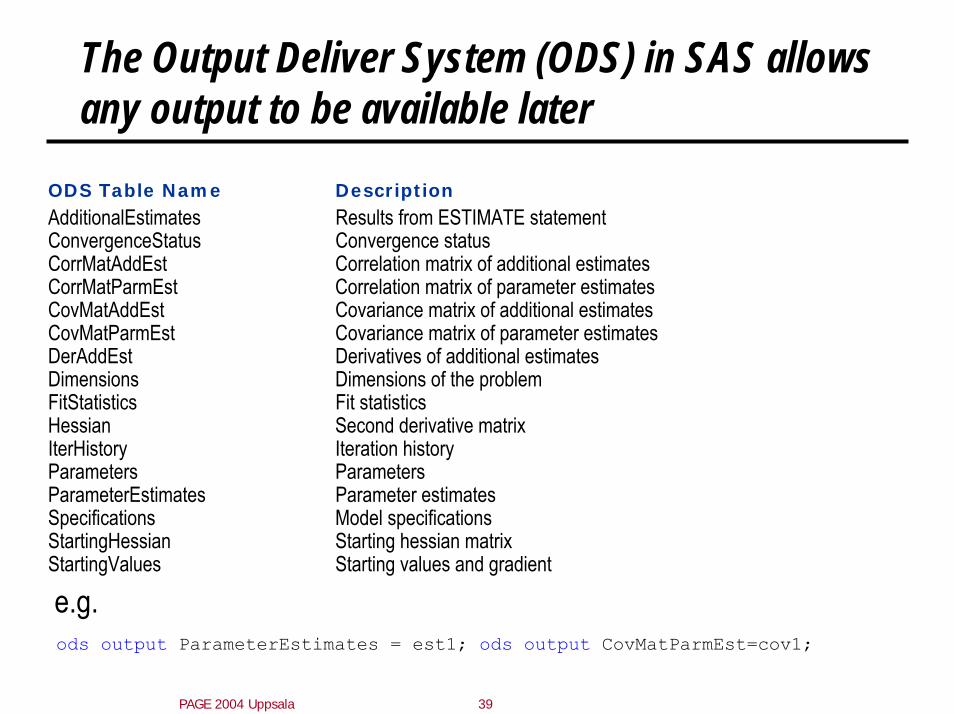
The Output Deliver System (ODS) in SAS allows any output to be available later
ODS Table Name DescriptionAdditionalEstimates Results from ESTIMATE statementConvergenceStatus Convergence statusCorrMatAddEst Correlation matrix of additional estimatesCorrMatParmEst Correlation matrix of parameter estimatesCovMatAddEst Covariance matrix of additional estimatesCovMatParmEst Covariance matrix of parameter estimatesDerAddEst Derivatives of additional estimatesDimensions Dimensions of the problemFitStatistics Fit statisticsHessian Second derivative matrixIterHistory Iteration historyParameters ParametersParameterEstimates Parameter estimatesSpecifications Model specificationsStartingHessian Starting hessian matrixStartingValues Starting values and gradient
ods output ParameterEstimates = est1; ods output CovMatParmEst=cov1;
e.g.
PAGE 2004 Uppsala 40
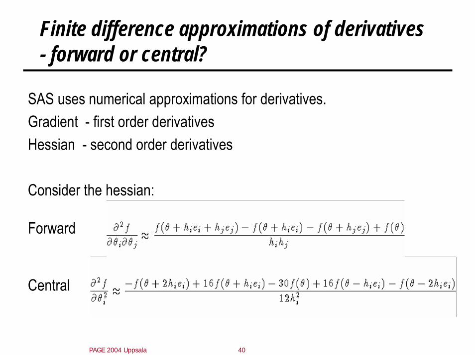
Finite difference approximations of derivatives - forward or central?
SAS uses numerical approximations for derivatives.Gradient - first order derivativesHessian - second order derivatives
Consider the hessian:
Forward
Central
PAGE 2004 Uppsala 41
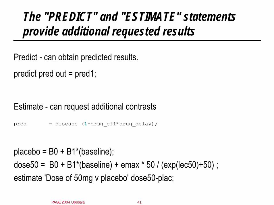
The "PREDICT" and "ESTIMATE" statements provide additional requested results
Predict - can obtain predicted results.
predict pred out = pred1;
Estimate - can request additional contrastspred = disease (1+drug_eff*drug_delay);
placebo = B0 + B1*(baseline);dose50 = B0 + B1*(baseline) + emax * 50 / (exp(lec50)+50) ; estimate 'Dose of 50mg v placebo' dose50-plac;

PAGE 2004 Uppsala 42
An example
Adaptive design
Using NLMIXED to determine the 'best' dose to allocate the next patient to, given a tentative model.
M&S has predicted target dose of Drug X to be between 1 and 200mg. 10 potential doses = 0 (placebo), 1, 2, 4, 8, 15, 30, 50,100, 200mg. Longitudinal model in place, developed on competitors in similar class.Initially, expect ED50 to be different for drug X, but similar Emax. Target - require 95% CI for log(ED50) to be within a 4 fold range.
PAGE 2004 Uppsala 43
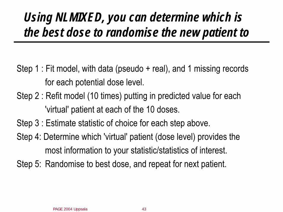
Using NLMIXED, you can determine which is the best dose to randomise the new patient to
Step 1 : Fit model, with data (pseudo + real), and 1 missing records for each potential dose level.
Step 2 : Refit model (10 times) putting in predicted value for each'virtual' patient at each of the 10 doses.
Step 3 : Estimate statistic of choice for each step above.Step 4: Determine which 'virtual' patient (dose level) provides the
most information to your statistic/statistics of interest. Step 5: Randomise to best dose, and repeat for next patient.

PAGE 2004 Uppsala 44
To give the model some initial stability, you create pseudo data.
Akin to priors in a bayesian sense. ED50 will depend on pseudo data at start of recruitment, but will not contribute at end.
Contribution of pseudo data to model
0
50
100
0 20 40 60 80 100 120 140 160 180 200
Patients Recruited
% c
ontri
butio
n to
mod
el
Pseudo Data Real Data
PAGE 2004 Uppsala 45
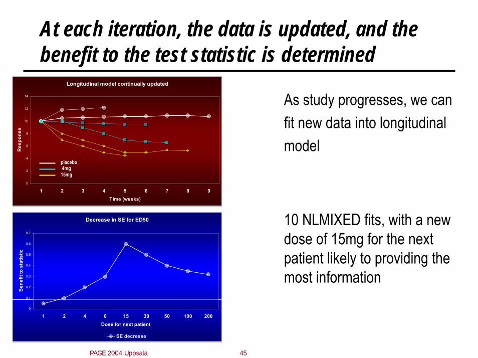
At each iteration, the data is updated, and the benefit to the test statistic is determined
Longitudinal model continually updated
0
2
4
6
8
10
12
14
1 2 3 4 5 6 7 8 9Time (weeks)
Res
pons
e
As study progresses, we can fit new data into longitudinal model
placebo4mg15mg
10 NLMIXED fits, with a new dose of 15mg for the next patient likely to providing the most information
Decrease in SE for ED50
0
0.1
0.2
0.3
0.4
0.5
0.6
0.7
1 2 4 8 15 30 50 100 200Dose for next patient
Ben
efit
to s
tatis
tic
SE decrease

PAGE 2004 Uppsala 46
Good coding methods - give the algorithms the best possible chance of being successful
RescalingCenteringReparameterisationEigenvalues