Nondestructive characterization of flake graphite cast iron by

Magnetic Adaptive Testing

Gábor Vértesy1, Tetsuya Uchimoto2, Toshiyuki Takagi2, Ivan Tomáš3 and Hidehiko

Kage4

1Hungarian Academy of Sciences, Institute of Technical Physics and Materials Science,

Budapest, Hungary

2Institute of Fluid Science, Tohoku University, Sendai, Japan

3 Center of Advanced and Innovative Technologies, VSB-TUO, Ostrava, Czech

Republic

4Kusaka Rare Metal Products Co., Tokyo, Japan

Abstract

Three series of flake graphite cast iron samples having different chemical compositions

and different heat treatments within each series were investigated by the method of

Magnetic Adaptive Testing. The flat samples were magnetized by an attached yoke, and

sensitive descriptors were obtained from the proper evaluation, based on the

measurements of series of magnetic minor hysteresis loops, without magnetic saturation

of the samples. Results of the non-destructive magnetic tests were compared with the

destructive mechanical measurements of Brinell hardness and linear correlation was

found between them in all cases, where the influence of chemical composition and

influence of heat treatment were considered.

Keywords: Cast iron, Magnetic hysteresis, Magnetic adaptive testing, Nondestructive

testing

Introduction

Cast iron is one of the most frequently used industrial construction materials. Low

cost of production, good machinability, and excellent possibilities of shaping the details

by casting attract an intense interest of industry. The cast irons are generally many-

component alloys of iron with large content of carbon. The cast iron structure is

classified by its metallic matrix composition (ferrite, pearlite, carbides, etc.) and by

morphology of its graphite inclusion. The mechanical properties are fundamentally

dependent both on the matrix composition and on the graphite shape (flaky, spheroidal,

vermicular, etc.), size and density [1]. One of the types of cast iron - the flake graphite

cast iron - is frequently used for mechanical components in bearings, brake shoes, etc.

because of its high wear resistance and damping capacity. The flake graphite cast iron is

an ideal material for automobile brake disks since it has excellent damping properties

and thermal conductivity just because of the flaky graphite.

The standard method of determining mechanical properties is the hardness test, in

which indentations are made from the surface to the core. This method is destructive

and time consuming. Because of this an easy nondestructive check-up of properties of

the cast iron is highly desired. Various non-destructive evaluation techniques have been

examined so far as an alternative method; alternating current potential drop [2], laser

acoustic wave [3], ultrasonic back-scattering [4], eddy currents [5-7], photothermal

radiometric radiometry [8].

Each technique gives indications of a good correlation between a measured physical

parameter and hardness.

Magnetic measurements are also frequently used for characterization of changes in

ferromagnetic materials, because magnetization processes are closely related to their

microstructure. This makes the magnetic approach an obvious candidate for non-

destructive testing, for detection and characterization of any defects in materials and in

products made of such materials [see e.g. 9]. The well known Barkhausen noise effect

can also be used for estimation of hardness in cast iron [10-13]. The so-called 3MA-

approach (micromagnetic, multiple-parameter, microstructure, and stress analysis) was

developed [14] in the last decade. This approach combines the information resulting

from the performance of different micromagnetic techniques (magnetic Barkhausen

noise, incremental permeability, harmonic analysis of the magnetic tangential field and

eddy current testing used at 3 different frequencies). By using the 3MA- method a

nondestructive hardness measurement is also possible [15].

A frequently and successfully used magnetic method is the measurement of

hysteresis loops. This method is mostly based on detection of structural variations via

the classical parameters of major hysteresis loops. Structural non-magnetic properties of

ferromagnetic materials have been non-destructively tested using traditional hysteresis

methods since long time with fair success. A number of techniques have been

suggested, developed and currently used in industry, for a review see e.g. [16].

Hardening of steel is measured by detection of B-H loops as published is some recent

works [17,18]. By applying this method, problems of non-destructive testing controlling

the structure of casting products were analyzed, too. Coercive force, residual

magnetization and saturation magnetization for white, gray, malleable and high-strength

cast irons at different structure of metallic matrices were measured. It was found that

measurement of the coercively sensitive magnetic parameter guarantees the quantitative

control of hardness of casts without surface cleaning [19,20].

An alternative, more sensitive and more experimentally friendly approach to this

topic was considered recently, based on magnetic minor loops measurement. The survey

of this technique can be found in [21]. The method called Magnetic Adaptive Testing

(MAT) was presented, which introduced general magnetic descriptors to diverse

variations in non-magnetic properties of ferromagnetic materials, optimally adapted to

the just investigated property and material. MAT was successfully applied for

characterization of material degradation in different specimens and it seems to be an

effective tool e.g. for replacement of the destructive hardness and/or ductile-brittle

transition temperature measurements.

In our previous works [22-24] magnetic characteristic parameters of a system of

minor loops, measured on a series of ductile cast iron samples, were analyzed, and their

sensitivity was evaluated. The flat samples were magnetized by an attached yoke and

sensitive parameters were obtained from the series of minor loops, without magnetic

saturation of the samples, which characterize well the samples’ structure. In a recent

work [25] MAT was applied for three flake graphite cast iron materials with different

chemical compositions and different matrix and flake graphite properties.

Metallographic examination of the matrix and the graphite structures was performed

and results of the non-destructive magnetic tests were compared with these data. A very

good correlation was found between the magnetic descriptors and the graphite

morphology. MAT was shown to be a useful tool for finding correlation between the

chosen nondestructively measured magnetic parameters and the graphite morphology.

Linear correlations with very small scatter of points were found between the optimally

chosen MAT degradation functions and both the graphite length and the graphite area of

the as-cast samples.

The purpose of the present work is to continue these measurements on three series

of flake graphite cast iron samples, to investigate the influence of both graphite

morphology structure and of matrices on mechanical and magnetic hardening, and to

find correlation between nondestructively measured magnetic parameters and

destructively determined Brinell hardness. We will also discuss the advantages of

Magnetic Adaptive Testing compared with other existing nondestructive magnetic

methods.

Samples

Three flake graphite cast iron materials with chemical compositions listed in

Table 1 were prepared.

Table 1.

Chemical composition of the flake graphite cast iron samples (values in wt%)

Sample Chemical composition CE

(%) C Si Mn P S Cr Ti

CE4.7 3.77 2.78 0.78 0.025 0.015 0.029 0.015 4.71

CE4.1 3.36 2.15 0.69 0.018 0.010 0.014 0.011 4.08

CE3.7 3.13 1.66 0.72 0.017 0.020 0.038 0.010 3.69

Their carbon equivalent (CE) values were defined by:

)P%massSi%mass(31C%mass ++=CE

and were controlled to produce various graphite shapes and sizes. These metals were

designated as CE4.7, CE4.1 and CE3.7 based on their targeted CE values. Pig iron

(4.09%C, 0.89%Si, 0.07%Mn, 0.019%P, 0.012%S, 0.016%Cr, 0.003%Ti), ferrosilicon

(Fe-75%Si), electrolytic iron and electrolytic manganese were used as raw materials and

were melted using a high frequency induction melting furnace at 1743 K. Ferrosilicon

(Fe-75%Si) was also used as an inoculant. The melts were poured into moulds made by

the CO2 gas process to produce the columnar bars with a length of 60 mm and a

diameter of 46 mm. Later each bar was cut into disks 10 mm thick. The disks were

subjected to two kinds of heat treatments: annealing to obtain a ferrite based matrix and

normalization to obtain a pearlite-based matrix. The disks intended for the heat

treatments were kept in a furnace at 850oC for one hour and then either cooled in the

furnace for the annealing or cooled in air for the normalization. We thus produced 3 as-

cast, 3 annealed and 3 normalized flake graphite cast iron materials with various

matrices and graphite shapes as shown in Table 2.

After grinding the specimen surfaces, their Brinell hardness HB (HBW 10/3000)

was measured and it is also listed in Table 2. These hardness values indicate that the

furnace-cooling and air-cooling treatments were successful in producing the ferritic and

pearlitic matrices, respectively.

Table 2.

Schedules of the heat treatment and the Brinell hardness (HBW)

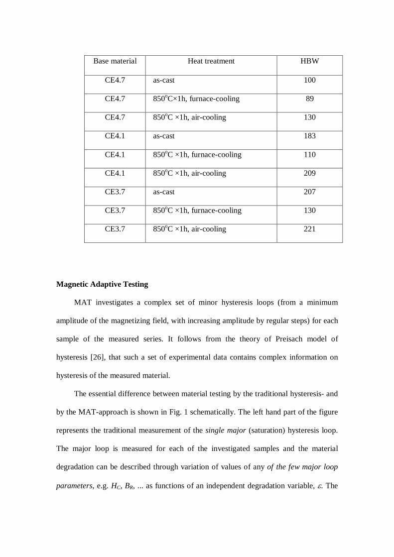
Base material Heat treatment HBW

CE4.7 as-cast 100

CE4.7 850oC×1h, furnace-cooling 89

CE4.7 850oC ×1h, air-cooling 130

CE4.1 as-cast 183

CE4.1 850oC ×1h, furnace-cooling 110

CE4.1 850oC ×1h, air-cooling 209

CE3.7 as-cast 207

CE3.7 850oC ×1h, furnace-cooling 130

CE3.7 850oC ×1h, air-cooling 221

Magnetic Adaptive Testing

MAT investigates a complex set of minor hysteresis loops (from a minimum

amplitude of the magnetizing field, with increasing amplitude by regular steps) for each

sample of the measured series. It follows from the theory of Preisach model of

hysteresis [26], that such a set of experimental data contains complex information on

hysteresis of the measured material.

The essential difference between material testing by the traditional hysteresis- and

by the MAT-approach is shown in Fig. 1 schematically. The left hand part of the figure

represents the traditional measurement of the single major (saturation) hysteresis loop.

The major loop is measured for each of the investigated samples and the material

degradation can be described through variation of values of any of the few major loop

parameters, e.g. HC, BR, ... as functions of an independent degradation variable, ε. The

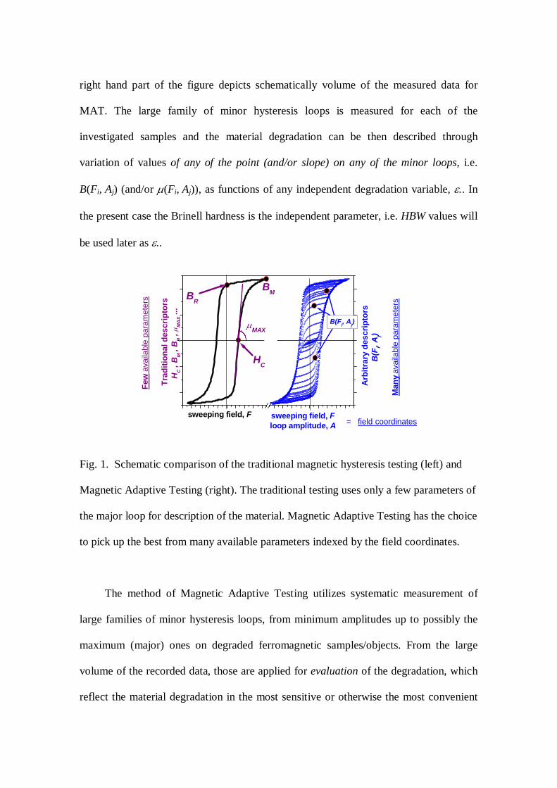
right hand part of the figure depicts schematically volume of the measured data for

MAT. The large family of minor hysteresis loops is measured for each of the

investigated samples and the material degradation can be then described through

variation of values of any of the point (and/or slope) on any of the minor loops, i.e.

B(Fi, Aj) (and/or µ(Fi, Aj)), as functions of any independent degradation variable, ε.. In

the present case the Brinell hardness is the independent parameter, i.e. HBW values will

be used later as ε..

B(Fi, Aj)

= field coordinates

µMAX

BMBR

HCA

rbitr

ary

desc

ripto

rsB

(Fi, A

j)

Man

y av

aila

ble

para

met

ers

sweeping field, F

Few

ava

ilabl

e pa

ram

eter

s

Trad

ition

al d

escr

ipto

rsH

C , B M

, B R ,

µ MA

X ...

sweeping field, Floop amplitude, A

Fig. 1. Schematic comparison of the traditional magnetic hysteresis testing (left) and

Magnetic Adaptive Testing (right). The traditional testing uses only a few parameters of

the major loop for description of the material. Magnetic Adaptive Testing has the choice

to pick up the best from many available parameters indexed by the field coordinates.

The method of Magnetic Adaptive Testing utilizes systematic measurement of

large families of minor hysteresis loops, from minimum amplitudes up to possibly the

maximum (major) ones on degraded ferromagnetic samples/objects. From the large

volume of the recorded data, those are applied for evaluation of the degradation, which

reflect the material degradation in the most sensitive or otherwise the most convenient

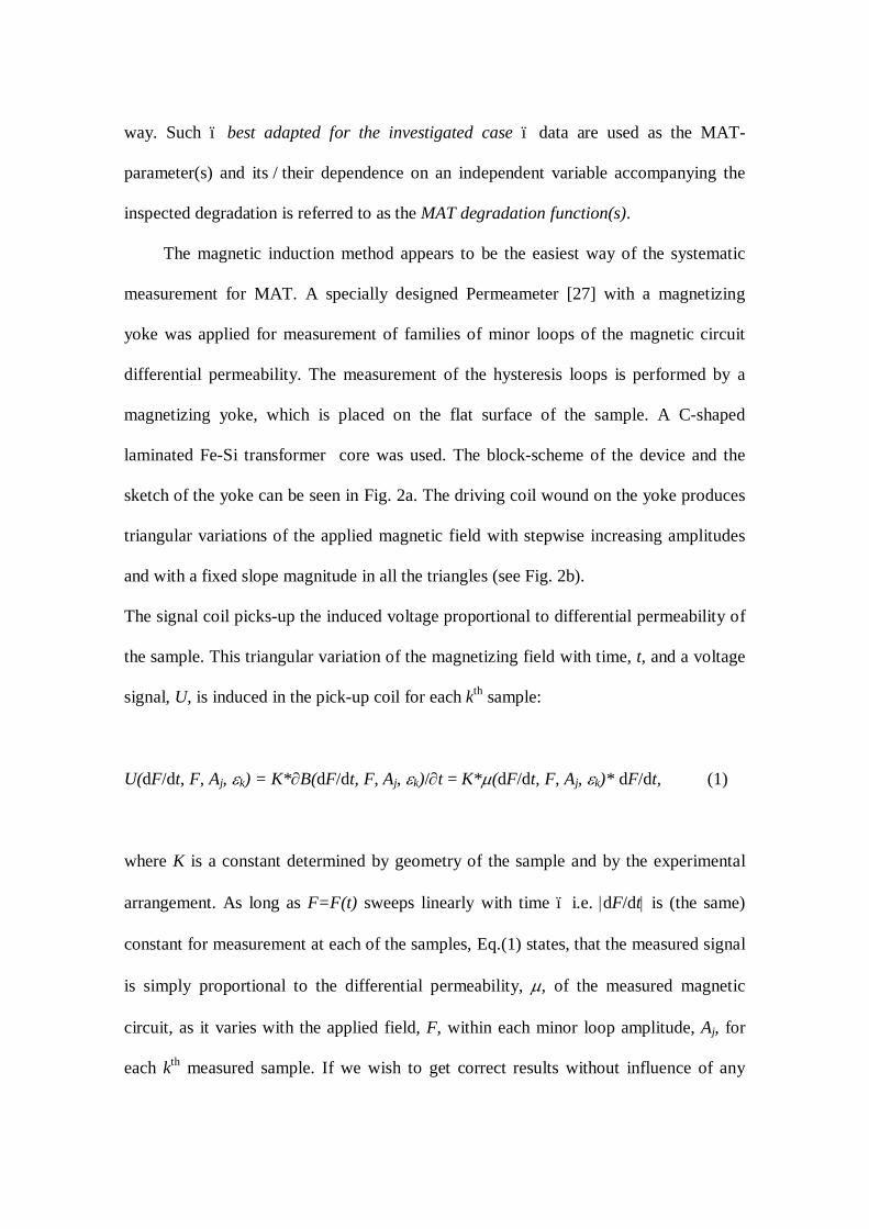
way. Such – best adapted for the investigated case – data are used as the MAT-

parameter(s) and its / their dependence on an independent variable accompanying the

inspected degradation is referred to as the MAT degradation function(s).

The magnetic induction method appears to be the easiest way of the systematic

measurement for MAT. A specially designed Permeameter [27] with a magnetizing

yoke was applied for measurement of families of minor loops of the magnetic circuit

differential permeability. The measurement of the hysteresis loops is performed by a

magnetizing yoke, which is placed on the flat surface of the sample. A C-shaped

laminated Fe-Si transformer core was used. The block-scheme of the device and the

sketch of the yoke can be seen in Fig. 2a. The driving coil wound on the yoke produces

triangular variations of the applied magnetic field with stepwise increasing amplitudes

and with a fixed slope magnitude in all the triangles (see Fig. 2b).

The signal coil picks-up the induced voltage proportional to differential permeability of

the sample. This triangular variation of the magnetizing field with time, t, and a voltage

signal, U, is induced in the pick-up coil for each kth sample:

U(dF/dt, F, Aj, εk) = K*∂B(dF/dt, F, Aj, εk)/∂t = K*µ(dF/dt, F, Aj, εk)* dF/dt, (1)

where K is a constant determined by geometry of the sample and by the experimental

arrangement. As long as F=F(t) sweeps linearly with time – i.e. |dF/dt| is (the same)

constant for measurement at each of the samples, Eq.(1) states, that the measured signal

is simply proportional to the differential permeability, µ, of the measured magnetic

circuit, as it varies with the applied field, F, within each minor loop amplitude, Aj, for

each kth measured sample. If we wish to get correct results without influence of any

previous remanence, it is evident that each sample has to be thoroughly demagnetized

before it is measured.

Com

puter

A/D

in/Out C

ard

Functiongenerator

Currentindication amplifier

Power amplifier

Signal amplifier

Sample

Signal coil

Resistor

Driving coil

Yoke

121.5 122.0 122.5 123.0 123.5 124.0-0.4

-0.3

-0.2

-0.1

0.0

0.1

0.2

0.3

0.4

Step, ∆IF

Mag

netiz

ing

curr

ent,

I F [A]

Time, t [a.u.]

a) b)

Fig. 2. a) Block-scheme of the Permeameter and sketch of the yoke, b) Triangular

variation of the magnetizing current with time.

The Permeameter works under control of a notebook PC, which sends the steering

information to the function generator and collects the measured data. An input/output

data acquisition card accomplishes the measurement. The computer registers actually

two data files for each measured family of the minor µ-shaped loops. The first one

contains detailed information about all the pre-selected parameters of the

demagnetization and of the measurement. The other file holds the course of the voltage

signal, U, induced in the pick-up coil as a function of time, t, and of the magnetizing

current, IF, and/or field, F. As an illustration, Fig. 3 presents the three families of

permeability loops, measured on the three as cast samples (CE3.7, CE4.1, CE4.7).

Evidently it is a lot of data and our task is to compare them and to find the most suitable

ones for characterizing the changes between samples.

-0,8 -0,6 -0,4 -0,2 0,0 0,2 0,4 0,6 0,8

-0,15

-0,10

-0,05

0,00

0,05

0,10

0,15

Pic

k-up

coi

l sig

nal,

U ~

µ ,

[mV

]

Magnetizing current, I, [A]

CE3.7CE4.1

CE4.7

As cast samples

Fig. 3. Examples of families of the µ-shaped loops vs. magnetizing current, IF,

measured on the three as cast samples. The positive and negative parts of the signal

correspond to the increasing and decreasing parts of the triangular waveform of the

current, respectively.

Instead of keeping the signal and the magnetizing field in shapes of continuous

time-dependent functions, it is practical to interpolate the family of data for each εk-

sample into a discrete square (i, j)-matrix, U(Fi, Aj, εk), with a suitably chosen step,

∆A = ∆F. (Because dF/dt is a constant, identical for all measurements within one

experiment, it is not necessary to write it explicitly as a variable of U.) MAT is a

relative method (practically all the nondestructive methods are relative), and the most

suitable information about degradation of the investigated material can be contained in

variation of any element, of such matrices as a function of ε, relative with respect to the

corresponding element of the reference matrix, U(Fi,Aj,ε0). So that we shall divide all

U(Fi, Aj, εk) elements by the corresponding elements U(Fi,Aj,ε0) of the reference sample

matrix and obtain normalized elements of matrices of relative differential permeability

µ(Fi,Aj,εk) = U(Fi, Aj, εk)/U(Fi, Aj, ε0), and their proper sequences

µ(Fi,Aj,ε) = U(Fi, Aj, ε)/U(Fi, Aj, ε0) (2)

as normalized µ-degradation functions of the inspected material.

In some cases it turns out, that degradation functions of reciprocal values, such

as 1/µ-degradation functions are more convenient than the direct ones. Application of

the reciprocal degradation functions proves effective especially in situations when –

with the increasing parameter ε – the direct degradation functions approach kind of a

“saturation”. Number of the degradation functions obtained from the MAT

measurement depends on magnitude of the maximum minor loop amplitude, Aj, up to

which the measurement is done, and on choice of the step value ∆A = ∆F which is used

for computation of the interpolated data matrices.

Once the degradation functions are computed, the next task is to find the

optimum degradation function(s) for the most sensitive and enough robust description of

the investigated material degradation. A 3D-plot of sensitivity of the degradation

functions can substantially help to choose the optimum one(s). For illustration, map of

relative sensitivity of the 1/µij(HBW)-degradation functions in the case of the as cast

samples is shown in Fig. 9. Slope of the linear regression of each degradation function

is here defined as the function sensitivity. Thus the sensitivity map is a 3D-graph of

these slope values plotted against the degradation functions field coordinates (Fi, Aj). As

it follows from the presented sensitivity maps, in Fig. 9 the most sensitive 1/µ-

degradation functions are those with field coordinates around (Fi=-700mA, Aj=725mA).

The most sensitive 1/µ-degradation functions are plotted in Fig. 6.

Size of the yoke was chosen to fit geometry of the samples: cross-section

S=10x5 mm2, the total outside length 18 mm, and the total outside height of the bow

22 mm. The magnetizing coil was wound on the bow of the yoke, with N=200 turns and

the pick-up (or signal) coil was wound on one of the yoke legs with n=75 turns.

Results

The metallographic examination of the matrix and graphite structures were done

according to ISO 945 [25]. Microphotographs of the three materials in their as-cast

condition revealed that the graphite flakes of CE4.7 are relatively long, they are

uniformly and isotropically distributed, and are thus categorized as type-B flakes

defined by ISO 945. CE4.1 has smaller graphite flakes than CE4.7 and they are

categorized as type-A flakes. In CE3.7 very small eutectic graphite flakes were found to

be distributed in the dendrite and they are categorized as type-D and type-E flakes.

Microphotographs of the samples after etching with 3% Nital indicated that CE4.7 had a

pearlite-ferrite matrix, CE3.7 had a completely pearlitic matrix, and CE4.1 mainly had a

pearlitic matrix and a small amount of ferrite surrounded the graphite flakes. The area

fraction and the average length of the graphite flakes were evaluated using an image

processing software. The area fraction of graphite was evaluated using microphotograph

binary images of 5 sample regions at the same magnification. The length of graphite is

defined as the average diameter of the minimum circle circumscribing each graphite

flake larger than 5 µm. The area fraction of graphite for CE4.7, CE4.1 and CE3.7 is

17.8, 12.6 and 10.0 %, respectively. The length of the graphite flakes for CE4.7, CE4.1

and CE3.7 is 67, 39 and 28 µm, respectively. For details see [25].

MAT degradation functions of all the investigated samples were evaluated and

those, optimized for description of the studied dependences, were considered as

functions of Brinell hardness. Optimization means that those µij(HBW)-degradation

functions were chosen from the big data pool, which were the most sensitive with

respect to the change of the independent parameter, and at the same time they were

highly repeatable, and in such a way the most reliable.

The results for the three different materials are given in Fig. 4. Here each graph

within the same figure represents one composition (CE4.7, CE4.1 and CE3.7) and the

type of cooling condition (as-cast, furnace-cooling, air-cooling) is also indicated. In

every case the MAT parameters are standardized by the corresponding value of the

sample within the same series, which has the lowest HBW. The optimum of MAT

descriptors in this case was the 1/µij(HBW)-degradation function, with (Fi = 0, Aj = 600

mA) values.

80 100 120 140 160 180 200 220 240

0,8

1,0

1,2

1,4

1,6

1,8

2,0

2,2

air cooling

as cast

furnace cooling

CE3.7

CE4.1

CE4.7

Brinell hardness

(FI =

0, A

J = 6

00 m

A) M

AT

desc

ripto

rs

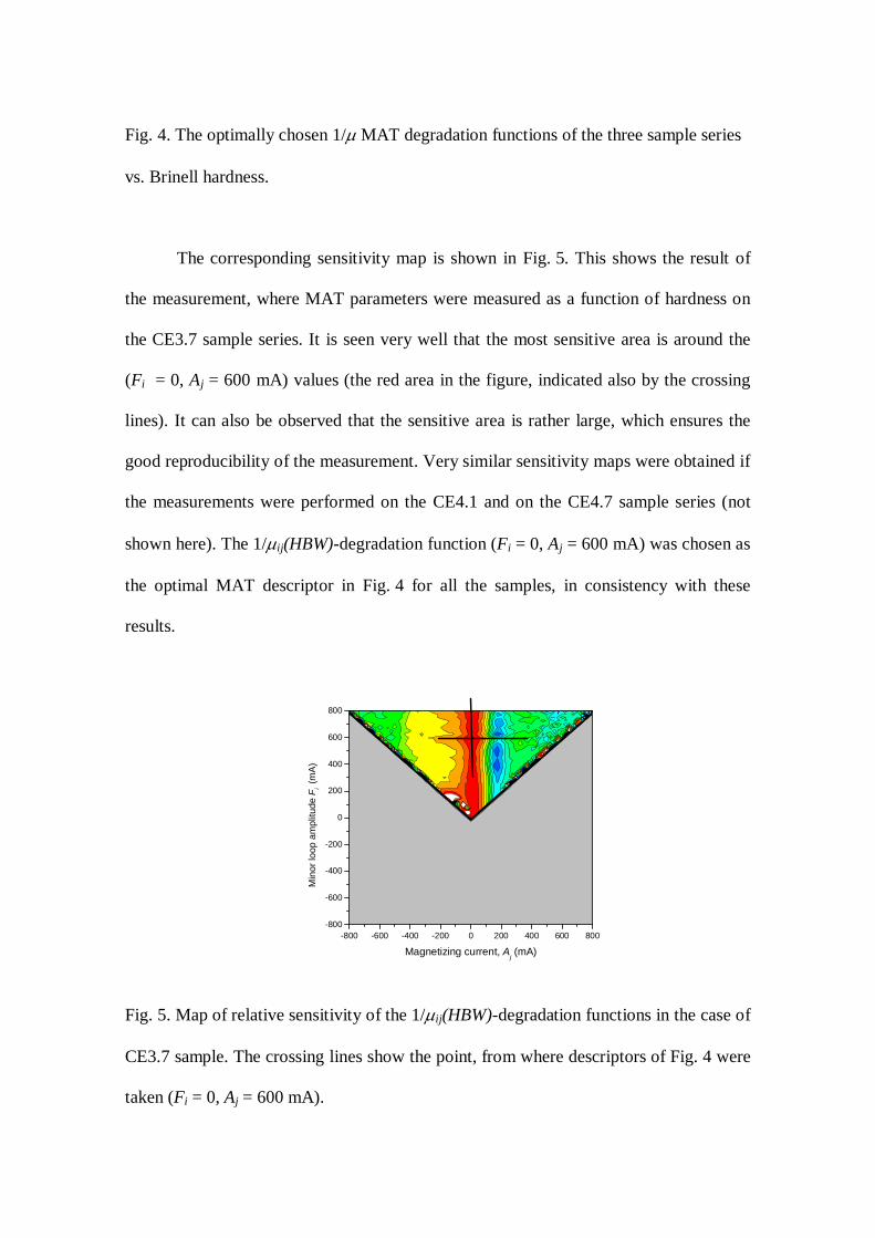
Fig. 4. The optimally chosen 1/µ MAT degradation functions of the three sample series

vs. Brinell hardness.

The corresponding sensitivity map is shown in Fig. 5. This shows the result of

the measurement, where MAT parameters were measured as a function of hardness on

the CE3.7 sample series. It is seen very well that the most sensitive area is around the

(Fi = 0, Aj = 600 mA) values (the red area in the figure, indicated also by the crossing

lines). It can also be observed that the sensitive area is rather large, which ensures the

good reproducibility of the measurement. Very similar sensitivity maps were obtained if

the measurements were performed on the CE4.1 and on the CE4.7 sample series (not

shown here). The 1/µij(HBW)-degradation function (Fi = 0, Aj = 600 mA) was chosen as

the optimal MAT descriptor in Fig. 4 for all the samples, in consistency with these

results.

-800 -600 -400 -200 0 200 400 600 800-800

-600

-400

-200

0

200

400

600

800

Magnetizing current, Aj (mA)

Min

or lo

op a

mpl

itude

Fi (

mA

)

Fig. 5. Map of relative sensitivity of the 1/µij(HBW)-degradation functions in the case of

CE3.7 sample. The crossing lines show the point, from where descriptors of Fig. 4 were

taken (Fi = 0, Aj = 600 mA).

.

The three graphs in Fig. 4 show the connection between the magnetic parameters

and the Brinell hardness within the same series (the same chemical composition) of the

samples. Different heat treatments result in different values of hardness.

However, the hardness (and simultaneously the magnetic parameters) are also

modified depending on graphite morphology, if the samples are prepared by the same

procedure (as-cast, furnace-cooling, air-cooling). The best MAT degradation functions

vs. Brinell hardness, optimized for the as cast samples, are shown in Fig. 6. The same is

shown in Fig. 7 and Fig. 8 for the furnace-cooled and for the air-cooled samples,

respectively. In all these cases (Figs. 6, 7 and 8) the optimum of MAT descriptor was

the 1/µij(HBW)-degradation function, with (Fi = -700 mA, Aj = 725 mA) values.

80 100 120 140 160 180 200 2200,8

1,0

1,2

1,4

1,6

1,8

2,0

2,2

2,4

as cast samplesCE4.7

CE4.1

CE3.7

F i =

-700

mA

, Aj =

725

mA

) M

AT

desc

ripto

rs

Brinell hardness

Fig. 6. The optimally chosen 1/µ MAT degradation function for the as-cast samples vs.

Brinell hardness.

80 90 100 110 120 130 1400,8

1,0

1,2

1,4

1,6

1,8

2,0

2,2

2,4

CE4.7

CE4.1

CE3.7

furnace cooled samples

Brinell hardness

F i =

-700

mA

, Aj =

725

mA

) M

AT

desc

ripto

rs

Fig. 7. The optimally chosen 1/µ MAT degradation function for the furnace-cooled

samples vs. Brinell hardness.

120 140 160 180 200 220 2400,8

1,0

1,2

1,4

1,6

1,8

2,0

2,2

2,4

2,6

2,8

CE4.7

CE4.1

CE3.7

(ha

= -7

00 m

A, h

b =

725

mA)

MAT

des

crip

tors

Brinell hardness

air cooled samples

Fig. 8. The optimally chosen 1/µ MAT degradation function for the air-cooled samples

vs. Brinell hardness.

The corresponding sensitivity map of Fig. 6 is shown in Fig. 9. This sensitivity

map shows the result of the measurement, where MAT parameters were measured as a

function of hardness on the three as cast samples. The most sensitive area is around (Fi

= -700 mA, Aj = 725 mA) values (the red area in the figure, indicated also by the

crossing lines). It can also be observed that the sensitive area is large enough, which

ensures the good reproducibility of the measurement. Very similar sensitivity maps

were obtained if the measurements were performed on the air cooled and on the furnace

cooled sample series. It means that in Figs. 6, 7 and 8 the optimally chosen MAT

descriptor is the 1/µij(HBW)-degradation function (Fi = -700 mA, Aj = 725 mA) for all

the three sample series.

-800 -600 -400 -200 0 200 400 600 800-800

-600

-400

-200

0

200

400

600

800

Magnetizing current, Aj (mA)

Min

or lo

op a

mpl

itude

Fi (m

A)

Fig. 9. Map of relative sensitivity of the 1/µij(HBW)-degradation functions in the case

of the as cast samples. The crossing lines show the point, from where descriptors of

Fig. 6 were taken (Fi = -700 mA, Aj = 725 mA).

Discussion

The samples are magnetized during the measurement by a magnetizing yoke,

which is placed on the flat surface of the sample. This experimental arrangement means

an open magnetic circuit, because some magnetic flux is always scattered at the air gap

between the yoke and the sample. To get reliable MAT-data, quality of the surface must

not vary from sample to sample and conditions of the measurement must be kept

constant within the each series of experiments. The exact value of the magnetic field

inside the sample is not known/measured in the used experimental arrangement.

Because of this, instead of the magnetic field (given in A/m), the value of the

magnetizing current (given in mA) is used as Fij and Aij when the µij ≡ µ( Fij, Aij) matrix

elements are given.

MAT parameters also depend on the microstructure state (graphite morphology),

because graphite morphology determines the pearlite-ferrite ratio of the material. This is

also very well reflected by magnetic measurements: very good correlation was found

between MAT parameters and graphite morphology. The correlation between MAT

parameters and both graphite length and graphite area was shown and discussed in Ref.

[25].

As it is seen in the figures, closely linear correlation was found between the

optimized MAT degradation functions and Brinell hardness in all the investigated cases.

It was applicable if the influence of different cooling conditions was investigated within

the same series of the samples (the same chemical composition, which leads to different

graphite structure), and also, if the influence of chemical composition was studied for

identically heat-treated samples. This confirms the fact that magnetic hardening follows

the mechanical hardening very well and that Magnetic Adaptive Testing is a powerful

tool for the nondestructive determination of this hardening.

There are several data in the literature about correlation between nondestructively

measured magnetic parameters (characteristics of major hysteresis loop, Barkhausen

noise measurements, etc.). In all cases a linear correlation was found between the

magnetic parameters and hardness [7,11,12,13,19,28]. This coincidence is rather

promising from that point of view, that magnetic measurements in general – regardless

on the actual type of investigation – reflect the changes in mechanical hardening and in

such a way they can replace the destructive and time consuming present standard way of

inspection. The question is, which magnetic measurement can be most successfully

applied. Based on our experience, we believe that MAT can be a suitable candidate for

future practical application. There are two important arguments, which support this

assumption. Our experience with previous MAT measurements, performed on different

samples showed that if different types of magnetic measurements (major hysteresis

loop, Barkhausen noise measurement) are applied on the same series of deformed

samples, MAT is more sensitive that other methods [21]. The other one is, that during

the MAT measurement there is no need for magnetic saturation of the investigated

sample, which is a big advantage. In practical applications, where big and complicated

shape samples should be measured, magnetic saturation is almost impossible.

We had alltogether nine samples, e.g. three series with three different samples

within each series. This means that the graphs contain only three measured points. From

the point of view of statistics this seems to be a rather low number, but considering the

large difference between the measured values, both in MAT parameters and hardness,

the low error of the measured points and the low scatter of points around the

hypothetical linear correlation, we believe that the results are reliable enough to prove

the correlation between magnetic parameters and independent parameter.

The above presented results reflect another important feature of Magnetic

Adaptive Testing, too. Namely its multiparametric character. Made one single

measurement on the investigated sample a big data pool is generated. The method of

Magnetic Adaptive Testing looks for those magnetic descriptors of the varied structural

properties, which are best adapted to the investigated property and to the investigated

material. It is seen on the above presented figures that different MAT descriptors were

used for characterization of material. If any series of samples with the same chemical

composition but with different thermal processing was considered, the 1/µij(HBW)-

degradation function with parameters (Fi = 0, Aj = 600 mA) gave good result. Another

1/µij(HBW)-degradation function with parameters (Fi = -700 mA, Aj = 725 mA)

reflected the hardness if different chemical composition samples with the same thermal

processing were considered. It is emphasized again that all of these degradation

functions were evaluated from one single measurement.

It is important to emphasize that MAT is a relative measurement: in all cases we

compare the parameters of measured samples with the parameters of the reference

(virgin) sample. For the successful application of the MAT method, first it is necessary

to make comparative, traditional, destructive measurements on a series of samples, for

“teaching” the MAT. This teaching procedure determines the optimum degradation

function/s, and the method of Magnetic Adaptive Testing is best adapted to the

investigated task in this way. Then, this/these chosen optimum degradation function(s)

will serve as sensitive calibration curve(s) for practical measurements on unknown

samples (of the same kind) to be investigated. Obviously different measuring conditions

result in different relative sensitivity of the calculated descriptors. Because of this

identical experimental conditions should be rigorously kept during measurement of the

tested objects, as they were applied during evaluation of the reference samples series. If

we do this, the reproducibility of the MAT parameters is excellent even replacing the

circuit after longer use in practice, and we detect only the material modification because

of the possible wear. The validity of this statement was tested by several control

measurements.

Conclusions

The method Magnetic Adaptive Testing, which is based on nondestructive,

systematic measurement of minor magnetic hysteresis loops was applied for three flake

graphite cast iron series having different chemical compositions and different heat

treatments within each series. MAT was shown to be a useful tool for finding

correlation between the nondestructively measured magnetic parameters and Brinell

hardness. Linear correlations with very small scatter of points were found between the

optimally chosen MAT degradation functions and the actual value of the Brinell

hardness, regardless if the chemical composition or the way of heat treatment was

considered. Also, referring to our previous work in this subject, good correlation was

found between MAT parameters and graphite morphology of as cast samples.

As a consequence, Magnetic Adaptive Testing proved to be an experimentally

friendly and sensitive method for nondestructive tests of the cast iron structure.

Acknowledgments

This work was partly supported by the JSPS Core-to-Core Program, „Advanced

Research Networks” (International research core on smart layered materials and

structures for energy saving), by Hungarian Scientific Research Fund (project

K 111662) and by the FY2013 Researcher Exchange Program between the Japan

Society for Promotion of Science and Hungarian Academy of Sciences. One of the co-

authors (I.T.) appreciates financial support by the project TA02011179 of the Technical

Agency of the Czech Republic.

References

[1] Walton CF, Opar TJ(Eds.), Iron casting handbook, Iron Casting Society, Inc., New

York, 1981.

[2] Bowler JR, Huang Y, Sun H, Brown J, Bowler N, Alternating current potential-

drop measurement of the depth of case hardening in steel rods, Measurement

Science and Technology 19 (2008) 075204.

[3] Schneider D, Hofmann R, Schwarz T, Grosser T, Hensel E, Evaluating surface

hardened steels by laser-acoustics Surface and Coatings Technology 206 (2012)

2079.

[4] Willems H, Review of Progress in Quantitative Nondestructive Evaluation 10B

(1991) 1707.

[5] Uchimoto T, Takagi T, Konoplyuk S, Abe T, Huang H, Kurosawa M, Eddy current

evaluation of cast iron for material characterization, J. Magn. Magn. Mater., 258-

259 (2003) 493.

[6] Konoplyuk S, Abe T, Uchimoto T, Takagi T, Kurosawa M, Characterization of

ductile cast iron by eddy current method, NDT&E International, 38 (2005) 623

[7] Feiste KL, Fetter Marques P, Reichert Ch, Reimche W, Stegemann D, Rebello

AJM, Krüger ES, Characterization of Nodular Cast Iron Properties by Harmonic

Analysis of Eddy Current Signals,

http://ndt.net/article/ecndt98/nuclear/245/245.htm

[8] Wang C, Mandelis A, Case depth determination in heat-treated industrial steel

products using photothermal radiometric interferometric phase minima, NDT&E

International 40 (2007) 158.

[9] Jiles DC, Magnetic methods in nondestructive testing, Buschow KHJ , Ed.,

Encyclopedia of Materials Science and Technology, Elsevier Press, Oxford, p.6021,

2001

[10] Santa-aho S, Vippola M, Sorsa A, Leiviskä K, Lindgren M, Lepistö T, Utilization

of Barkhausen noise magnetizing sweeps for case-depth detection from hardened

steel, NDTE&E International, 52 (2012) 95-102

[11] Helmersson PL, Thibblin A, Method for handling a cast iron component based on

estimating hardness by magnetic Barkhausen noise, USPTO Application

#:#20080238418 - Class: 324234 (USPTO) - 10/02/08 - Class 324

[12] Pirfo Barroso S, Horváth M, Horváth Á, Magnetic measurements for evaluation of

radiation damage on nuclear reactor materials, Nuclear Engineering and Desing

240 (2010) 722-725

[13] Luo XY, Zhang Y, Wang ZJ, Zhang YS, Non-destructive Testing Device for Hot

Forming High Strength Steel Parts Based on Barkhausen Noise, Applied Materials

and Technologies for Modern Manufacturing, PTS 1-4, 2013, Volume: 423-426,

pp. 2555-2558

[14] Dobmann G, (2011). Non-Destructive Testing for Ageing Management of

Nuclear Power Components, Nuclear Power - Control, Reliability and Human

Factors, Dr. Pavel Tsvetkov (Ed.), ISBN: 978-953-307-599-0, InTech, DOI:

10.5772/17581. Available from: http://www.intechopen.com/books/nuclear-

power-control-reliability-and-human-factors/non-destructive-testing-for-ageing-

management-of-nuclear-power-components

[15] Altpeter I, Becker R, Dobmann G, Kern R, Theiner A, Yashan A, Robust solutions

of inverse problems in electromagnetic non-destructive evaluation, Inverse

Problems, 18 (2002) 1907-1921

[16] Blitz J, Electrical and magnetic methods of nondestructive testing, Bristol, Adam

Hilger IOP Publishing, Ltd., 1991.

[17] Zhang C, Bowler N, Lo C, Magnetic characterization of surface-hardened steel, J.

Magn. Magn. Mater, 321 (2009) 3878–3887

[18] Kobayashi S,Takahashi S, Kamada Y, Evaluation of case-depth in induction-

hardened steels: Magnetic hysteresis measurements and hardness-depth profiling

by differential permeability analysis, J. Magn. Magn. Mater., 343 (2013) 112-118

[19] Sandomirsky SG, Magnetic testing of structure of the cast-iron products:

possibilities and results, www.ndt.net/article/ecndt2010/reports/1_01_21.pdf

[20] Sandomirsky SG, Tsukerman VL, Pisarenko LZ, Possibilities and results of

hardness control of cast iron castings by magnetic method after polar

magnetization, Foundry production and Metallurgy (Литье и Метaллургия), No.

3 (2007) pp. 106-110

[21] Tomáš I, Vértesy G, Magnetic Adaptive Testing, in Nondestructive Testing

Methods and New Applications, M.Omar (Ed.), ISBN: 978-953-51-0108-6,

(2012), InTech: http://www.intechopen.com/articles/show/title/magnetic-adaptive-

testing.

[22] Vértesy G, Uchimoto T, Takagi T, Tomáš I, Stupakov O, Meszaros I, Pavo J,

Minor hysteresis loops measurements for characterization of cast iron, Physica B,

372 (2006), pp. 156-159

[23] Vértesy G, Uchimoto T, Tomáš I, Takagi T, Nondestructive characterization of

ductile cast iron by Magnetic Adaptive Testing, J.Magn.Magn.Mater. 322 (2010)

3117-3121.

[24] Tomáš I, Skrbek B, Uchimoto T, Kadlecová J, Stupakov O, Perevertov O, Dočekal

J, Application of Magnetic Adaptive Testing to Cast Iron, Acta Metallurgica

Slovaca, 13 (2007) pp.129 – 132.

[25] Vértesy G, Uchimoto T, Takagi T, Tomáš I, Flake graphite cast iron investigated

by a magnetic method, IEEE Trans. Magn, Vol. 50. No. 4, April 2014, 6200404

[26] Mayergoyz ID, Mathematical models of hysteresis, Springer-Verlag, New York,

1991

[27] Tomáš I, Perevertov O, Permeameter for Preisach approach to materials testing,

JSAEM Studies in Applied Electromagnetics and Mechanics 9, Ed. Takagi T,

Ueasaka M, IOS Press, Amsterdam, p. 5., 2001.

[28] Fillion G, Lord M, Bussiere JF, Inference of hardness from magnetic measurement

on pearlitic steels, Review of Progress in Quantitative Nondestructive Evaluation,

Vol. 9, Eds. Thomson DO, Climenti DE, Plenum Press, New York, 1990

Figure captions

Fig. 1: Schematic comparison of the traditional magnetic hysteresis testing (left) and

Magnetic Adaptive Testing (right). The traditional testing uses only a few

parameters of the major loop for description of the material. Magnetic Adaptive

Testing has the choice to pick up the best from many available parameters

indexed by the field coordinates.

Fig. 2: a) Block-scheme of the Permeameter and sketch of the yoke, b) Triangular

variation of the magnetizing current with time.

Fig. 3: Examples of families of the µ-shaped loops vs. magnetizing current, IF,

measured on the three as cast samples. The positive and negative parts of the

signal correspond to the increasing and decreasing parts of the triangular

waveform of the current, respectively.

Fig. 4: The optimally chosen 1/µ MAT degradation functions of the three sample series

vs. Brinell hardness.

Fig. 5: Map of relative sensitivity of the 1/µij(HBW)-degradation functions in the case of

CE3.7 sample. The crossing lines show the point, from where descriptors of

Fig. 4 were taken (Fi = 0, Aj = 600 mA).

Fig. 6: The optimally chosen 1/µ MAT degradation function for the as-cast samples vs.

Brinell hardness.

Fig. 7: The optimally chosen 1/µ MAT degradation function for the furnace-cooled

samples vs. Brinell hardness.

Fig. 8: The optimally chosen 1/µ MAT degradation function for the air-cooled samples

vs. Brinell hardness.

Fig. 9: Map of relative sensitivity of the 1/µij(HBW)-degradation functions in the case of

the as cast samples. The crossing lines show the point, from where descriptors of

Fig. 6 were taken (Fi = -700 mA, Aj = 725 mA).