noninvasive estimation of pulmonary artery pressure using
TRANSCRIPT
Brigham Young University Brigham Young University
BYU ScholarsArchive BYU ScholarsArchive
Theses and Dissertations
2009-12-07
Noninvasive Estimation of Pulmonary Artery Pressure Using Heart Noninvasive Estimation of Pulmonary Artery Pressure Using Heart
Sound Analysis Sound Analysis
Aaron W. Dennis Brigham Young University - Provo
Follow this and additional works at: https://scholarsarchive.byu.edu/etd
Part of the Computer Sciences Commons
BYU ScholarsArchive Citation BYU ScholarsArchive Citation Dennis, Aaron W., "Noninvasive Estimation of Pulmonary Artery Pressure Using Heart Sound Analysis" (2009). Theses and Dissertations. 1971. https://scholarsarchive.byu.edu/etd/1971
This Thesis is brought to you for free and open access by BYU ScholarsArchive. It has been accepted for inclusion in Theses and Dissertations by an authorized administrator of BYU ScholarsArchive. For more information, please contact [email protected], [email protected].

Noninvasive Estimation of Pulmonary Artery Pressure
Using Heart Sound Analysis
Aaron Dennis
A thesis submitted to the faculty ofBrigham Young University
in partial fulfillment of the requirements for the degree of
Master of Science
Dan Ventura, ChairTony MartinezSean Warnick
Department of Computer Science
Brigham Young University
April 2010
Copyright c© 2010 Aaron Dennis
All Rights Reserved
ABSTRACT
Noninvasive Estimation of Pulmonary Artery Pressure
Using Heart Sound Analysis
Aaron Dennis
Department of Computer Science
Master of Science
Right-heart catheterization is the most accurate method for estimating pulmonaryartery pressure (PAP). Because it is an invasive procedure it is expensive, exposes patientsto the risk of infection, and is not suited for long-term monitoring situations. Medicalresearchers have shown that PAP influences the characteristics of heart sounds. Thissuggests that heart sound analysis is a potential noninvasive solution to the PAP estimationproblem.
This thesis describes the development of a prototype system, called PAPEr, whichestimates PAP noninvasively using heart sound analysis. PAPEr uses patient data withmachine learning algorithms to build models of how PAP affects heart sounds. Data from20 patients was used to build the models and data from another 31 patients was used asa validation set. PAPEr diagnosed these 31 patients for pulmonary hypertension with anaccuracy of 77 percent.
Keywords: machine learning, pulmonary artery pressure estimation, feature selection

ACKNOWLEDGMENTS
I would like to thank my advisor, Dr. Dan Ventura, for pointing me to this project,
funding my work, and for discussing with me many of the issues and problems that arose
while completing this thesis.
Dr. Andrew Michaels from the University of Utah Health Sciences Center initiated
the PAP estimation project and invited us to be involved. His team also recorded the patient
data used in this thesis.
Patti Arand from Invose Medical, Inc. sent us the patient data along with invaluable
measurements that were calculated from the patient data using software developed at Inovise.
Dr. Michaels and Patti both took part in fruitful discussions with us and provided
helpful reading material, including articles from the medical literature, information about
the operation of the Audicor machine, and useful background information. Many thanks to
both of them for their help.
My lovely wife Maren and my brother William both read a version of this thesis and
their suggestions have improved its clarity and grammar. Thanks to them from me and from
Dr. Ventura, who was spared wading through that earlier and messier draft. Maren has also
given me the support and encouragement I needed as well as an intelligent listening ear.

Contents
List of Figures vi
List of Tables vii
1 Introduction 1
1.1 Background . . . . . . . . . . . . . . . . . . . . . . . . . . . . . . . . . . . . 1
1.1.1 Heart Structure . . . . . . . . . . . . . . . . . . . . . . . . . . . . . . 2
1.1.2 Heart Sounds . . . . . . . . . . . . . . . . . . . . . . . . . . . . . . . 3
1.1.3 Pulmonary Hypertension . . . . . . . . . . . . . . . . . . . . . . . . . 3
1.1.4 Measuring Pulmonary Artery Pressure . . . . . . . . . . . . . . . . . 4
1.1.5 Machine Learning in Medicine . . . . . . . . . . . . . . . . . . . . . . 5
1.2 What Others Have Done . . . . . . . . . . . . . . . . . . . . . . . . . . . . . 6
1.3 Our Approach . . . . . . . . . . . . . . . . . . . . . . . . . . . . . . . . . . . 8
1.4 Some Terminology . . . . . . . . . . . . . . . . . . . . . . . . . . . . . . . . 9
1.5 Thesis Overview . . . . . . . . . . . . . . . . . . . . . . . . . . . . . . . . . . 10
2 System Design Space 11
2.1 Patient Measurements . . . . . . . . . . . . . . . . . . . . . . . . . . . . . . 11
2.1.1 Data Collection . . . . . . . . . . . . . . . . . . . . . . . . . . . . . . 11
2.1.2 Inovise Features . . . . . . . . . . . . . . . . . . . . . . . . . . . . . . 12
2.1.3 Heart Sound Features . . . . . . . . . . . . . . . . . . . . . . . . . . . 14
2.2 Learning Algorithms . . . . . . . . . . . . . . . . . . . . . . . . . . . . . . . 16
2.2.1 Decision Tree (J48) . . . . . . . . . . . . . . . . . . . . . . . . . . . . 17
iv

2.2.2 K-Nearest Neighbors (KNN) . . . . . . . . . . . . . . . . . . . . . . . 17
2.2.3 Multilayer Perceptron (MLP) . . . . . . . . . . . . . . . . . . . . . . 17
2.2.4 Naive Bayes (NB) . . . . . . . . . . . . . . . . . . . . . . . . . . . . . 18
2.2.5 Support Vector Machine (SMO) . . . . . . . . . . . . . . . . . . . . . 18
3 Experiments 19
3.1 System Configuration . . . . . . . . . . . . . . . . . . . . . . . . . . . . . . . 19
3.2 Evaluating Configurations . . . . . . . . . . . . . . . . . . . . . . . . . . . . 20
3.3 Feature Subset Selection . . . . . . . . . . . . . . . . . . . . . . . . . . . . . 22
3.3.1 Greedy Forward-Selection Search . . . . . . . . . . . . . . . . . . . . 23
3.3.2 Feature Ranking . . . . . . . . . . . . . . . . . . . . . . . . . . . . . 24
3.4 Exhaustive Bootstrapping . . . . . . . . . . . . . . . . . . . . . . . . . . . . 25
3.5 Validation . . . . . . . . . . . . . . . . . . . . . . . . . . . . . . . . . . . . . 26
4 Results 28
4.1 GFS Search Results . . . . . . . . . . . . . . . . . . . . . . . . . . . . . . . . 28
4.2 Ranked Feature List . . . . . . . . . . . . . . . . . . . . . . . . . . . . . . . 33
4.3 Configuration Evaluations . . . . . . . . . . . . . . . . . . . . . . . . . . . . 34
4.4 Overall Performance . . . . . . . . . . . . . . . . . . . . . . . . . . . . . . . 35
4.5 Holdout Set Classification . . . . . . . . . . . . . . . . . . . . . . . . . . . . 38
5 Conclusion 41
References 44
v

List of Figures
1.1 Structure of the Heart . . . . . . . . . . . . . . . . . . . . . . . . . . . . . . 2
1.2 PAPEr System Overview . . . . . . . . . . . . . . . . . . . . . . . . . . . . . 8
3.1 Experiments Overview . . . . . . . . . . . . . . . . . . . . . . . . . . . . . . 20
4.1 Greedy Forward-Selection Searches . . . . . . . . . . . . . . . . . . . . . . . 29
4.2 Exhaustive Bootstrapping Results . . . . . . . . . . . . . . . . . . . . . . . . 35
4.3 ROC Curves from 25 Configuration Evaluations . . . . . . . . . . . . . . . . 36
4.4 Location Performance . . . . . . . . . . . . . . . . . . . . . . . . . . . . . . 37
4.5 Learner Performance . . . . . . . . . . . . . . . . . . . . . . . . . . . . . . . 38
4.6 Feature Performance . . . . . . . . . . . . . . . . . . . . . . . . . . . . . . . 39
vi

List of Tables
2.1 Definitions of Heart Sound Event Variables . . . . . . . . . . . . . . . . . . . 13
2.2 Heart Sound Features . . . . . . . . . . . . . . . . . . . . . . . . . . . . . . . 15
4.1 Features Selected by the Greedy Forward-Selection Searches 1 . . . . . . . . 30
4.2 Features Selected by the Greedy Forward-Selection Searches 2 . . . . . . . . 31
4.3 Features Selected by the Greedy Forward-Selection Searches 3 . . . . . . . . 32
4.4 Ranked Feature List . . . . . . . . . . . . . . . . . . . . . . . . . . . . . . . 34
4.5 Validation Results: Sensitivity and Specificity . . . . . . . . . . . . . . . . . 39
4.6 Validation Results: Accuracy and AUC . . . . . . . . . . . . . . . . . . . . . 40
vii

Chapter 1
Introduction
This thesis describes the development of a prototype system that estimates pulmonary
artery pressure (PAP) noninvasively. Current invasive techniques are expensive and expose
patients to the risk of infection. Current noninvasive techniques cannot be used on many
patients. The prototype system described here uses machine learning techniques to analyze
features of heart sound recordings in order to produce PAP estimates. Analysis of heart
sounds is a noninvasive method that can be applied to the great majority of patients, if not
all of them. Using heart sound analysis to approach the problem of PAP estimation was
motivated by studies that have shown a correlation between PAP and various heart sound
features.
1.1 Background
The following subsections briefly present information about the structural and functional
anatomy of the heart, pulmonary hypertension, approaches for measuring or estimating PAP,
and the application of machine learning to medical problems in general. This information is
helpful in understanding the problem of noninvasive PAP estimation and in understanding
our general approach to the problem.
1
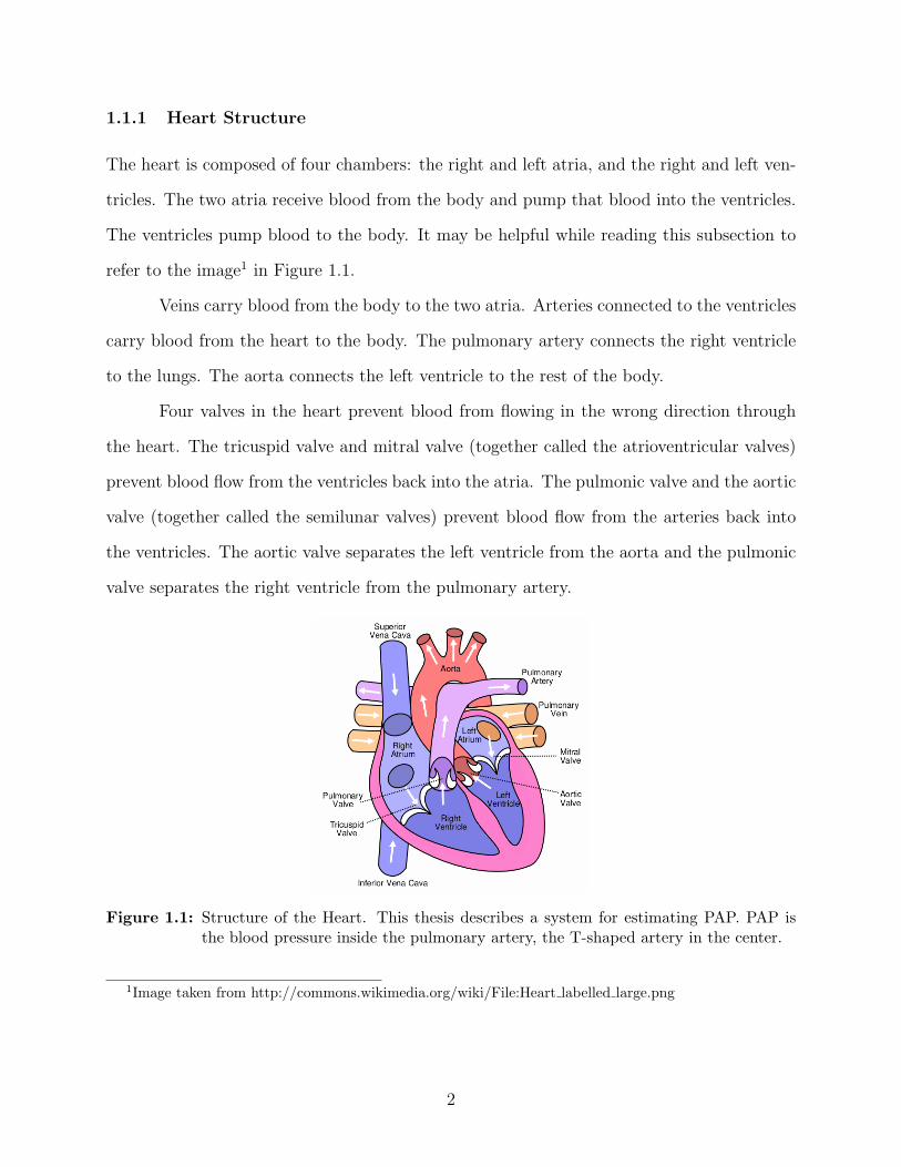
1.1.1 Heart Structure
The heart is composed of four chambers: the right and left atria, and the right and left ven-
tricles. The two atria receive blood from the body and pump that blood into the ventricles.
The ventricles pump blood to the body. It may be helpful while reading this subsection to
refer to the image1 in Figure 1.1.
Veins carry blood from the body to the two atria. Arteries connected to the ventricles
carry blood from the heart to the body. The pulmonary artery connects the right ventricle
to the lungs. The aorta connects the left ventricle to the rest of the body.
Four valves in the heart prevent blood from flowing in the wrong direction through
the heart. The tricuspid valve and mitral valve (together called the atrioventricular valves)
prevent blood flow from the ventricles back into the atria. The pulmonic valve and the aortic
valve (together called the semilunar valves) prevent blood flow from the arteries back into
the ventricles. The aortic valve separates the left ventricle from the aorta and the pulmonic
valve separates the right ventricle from the pulmonary artery.
Figure 1.1: Structure of the Heart. This thesis describes a system for estimating PAP. PAP isthe blood pressure inside the pulmonary artery, the T-shaped artery in the center.
1Image taken from http://commons.wikimedia.org/wiki/File:Heart labelled large.png
2

1.1.2 Heart Sounds
Ventricular systole is the phase of the cardiac cycle in which both ventricles contract, ejecting
blood into the arteries. At the beginning of systole, pressure in the ventricles rises above
the pressure in the atria, pushing the two atrioventricular valves shut. The closing of these
valves coincides with the first heart sound (S1). At the end of systole, the ventricles begin
to relax and the pressure in the ventricles drops below the pressure in the arteries, pushing
the two semilunar valves shut. The closing of these valves coincides with the second heart
sound (S2).
Pressure differences across heart valves accelerate columns of blood against the valves
forcing them shut. The closing of the valves stops (or rapidly decelerates) the flow of blood.
This rapid acceleration and deceleration of blood causes the heart and surrounding tissues
to vibrate, producing the heart sounds. It is easy to think that the heart valves snapping
shut produce the heart sounds just as slapping your hands together produces a sound. In
actuality the flow of blood against the valves and its interaction with the elastic tissues in
the heart produce the heart sounds.
The S1 is composed of two overlapping components, called M1 and T1. M1 is the
component of S1 that coincides with the closure of the mitral valve and T1 is the component
that coincides with the closure of the tricuspid valve.
Similarly, the S2 is composed of two overlapping components, called P2 and A2. P2
is the component of S2 that coincides with the closure of the pulmonic valve and A2 is the
component that coincides with the closure of the aortic valve.
1.1.3 Pulmonary Hypertension
Pulmonary hypertension is high blood pressure in the pulmonary artery. It “begins when
tiny arteries in your lungs, called pulmonary arteries and capillaries, become narrowed,
blocked or destroyed. This makes it harder for blood to flow through your lungs, which
raises pressure within the pulmonary arteries” (15). Narrowed, blocked, or destroyed pul-
3

monary blood vessels are caused by blood clots, emphysema, cleroderma, and other diseases.
Pulmonary hypertension can cause “heart muscle to weaken and sometimes fail completely”
(15). Treatments for pulmonary hypertension are available.
1.1.4 Measuring Pulmonary Artery Pressure
“The pulmonary artery pressure (PAP) is a very useful parameter for the clinical evaluation
of many cardiac diseases” (1). Several methods have been developed to measure PAP. Right-
heart catheterization gives the most accurate PAP measurement, but has many drawbacks
because it is an invasive procedure. Doppler echocardiography is a noninvasive technique
for PAP measurement, but it cannot be used with all patients. Heart sound analysis is a
promising, but still experimental method of estimating PAP.
Right-Heart Catheterization
Right-heart catheterization gives the most reliable and accurate measurement of PAP (1)(15).
It is performed by threading a Swan-Ganz catheter through a vein until it reaches the
pulmonary artery. At this point a PAP measurement can be made. Disadvantages of this
approach include high expense, risk of infection, and risk of physical harm to internal bodily
structures.
Doppler Echocardiography
Doppler echocardiography uses ultrasound technology and the Doppler effect to measure the
speed and direction of blood flow within the heart. Doppler echocardiography is noninvasive,
safe, and relatively cheap. The disadvantage is that it cannot be used to estimate PAP “in
approximately 50% of patients with normal PAP, 10-20% of patients with increased PAP,
and 34-76% of patients with chronic obstructive pulmonary disease” (19).
4

Heart Sound Analysis
Theoretical considerations as well as experimental results (1)(4)(19) point to a relationship
between PAP and heart sounds. For example, Aggio notes that “the pressure levels in
the pulmonary artery are known to influence the characteristics of the second heart sound
(S2): a rise of PAP is associated with an enhancement of its pulmonary component” (1).
The existence of the PAP/heart sound relationship makes it possible to estimate PAP (and
diagnose pulmonary hypertension) by analyzing heart sounds.
Heart sound analysis is a promising technique for noninvasive PAP estimation. The
approach taken by the heart sound analysis system described in this thesis is to record a
patient’s heart sound, extract heart sound features that are predictive of PAP, and produce
a PAP estimate from these extracted features using a machine learning classifier.
Heart sound analysis is noninvasive, inexpensive, safe, can be used on most if not all
patients, and may be automated using computer software. In short, it has the potential to
provide PAP estimates without the disadvantages of right-heart catheterization and Doppler
echocardiography. However, heart sound analysis is still in an experimental stage and has
not yet matured enough to replace the other methods of PAP estimation.
1.1.5 Machine Learning in Medicine
Artificial intelligence and machine learning methods have been used for decades to address
problems in medicine. Areas in which these methods are currently used include diagnosis,
laboratory testing, education, medical image analysis, and administration (5, chapter 25).
Many specific applications of machine learning algorithms can be found in the literature,
some of which are discussed in (9) and (14).
A wide range of machine learning algorithms have been used to address various medi-
cal problems. These include naive Bayes, neural networks, symbolic learning, expert systems,
belief networks, decision trees, support vector machines, Bayesian networks, and generative
models (5)(9)(14).
5

We have used machine learning algorithms in approaching the problem of PAP esti-
mation. One of the reasons for using machine learning in this context is that the relationship
between PAP and heart sounds is not fully understood and may be quite complex. Because
the relationship is not fully understood, we cannot use an analytical solution. Machine
learning algorithms can be trained using patient data to produce complex models of the
PAP/heart sound relationship.
1.2 What Others Have Done
Several studies have examined the relationship between S2 and PAP. The ideas, methods,
and heart sound features used in these studies provide a starting point for this thesis.
Most studies of S2 and PAP have been carried out by medical researchers. Typically
the researchers will record heart sound data from test subjects (human patients and/or pigs)
while simultaneously measuring the test subject’s PAP using right-heart catheterization.
Then they extract from the heartbeat sounds various features that are hypothesized to be
predictive of PAP. In this way they create a database of PAP values paired with heartbeat
sound feature values. They then fit a curve (either explicitly or implicitly) to the data using
PAP as the dependent variable and the features as the independent variables. The researchers
use the curve to model the data. Using statistical measures such as the correlation coefficient
they determine how well the curve-based model explains the data.
The approach taken in this thesis is different from the approach described in the
previous paragraph. We used machine learning algorithms to infer models of the data instead
of curve fitting. We used the models to classify test data instead of measuring the correlation
between a model and the data. Classifying test data provides us with an estimate of the
model’s predictive accuracy. We will call our approach the machine learning approach. We
will call the other approach the statistical approach.
One of the goals of either approach is to determine which features or feature com-
binations can and cannot be used to build good models of the data. Aggio et al. studied
6

various characteristics of the frequency spectrum of the P2 component of S2 (1). Chen,
Pibarot, Honos, and Durand looked at additional S2 frequency spectrum characteristics (4).
Xu, Durand, and Pibarot looked at the splitting interval between the A2 and P2 sounds (19).
Tranulis, Durand, Senhadji, and Pibarot used a time-frequency representation of the second
heart sound to train a multilayer perceptron for PAP estimation and patient diagnosis (16).
Many of the features from these studies will be used in this thesis (see Section 2.1.3 for
specifics).
A machine learning approach was used in (16), which distinguishes it from the other
studies. This study built a model of the data using a machine learning algorithm (the
multilayer perceptron), classified a test set of data, and reported classification accuracies
for the model. However, the reported results are overly optimistic—at least they are if the
classification accuracies were intended as an estimate of how well their model would perform
on real-world patients.
The reason for the overly optimistic results is that all data from a single test subject
was not grouped together. Instead, the heartbeat sounds from a single test subject were
randomly shuffled and then split into two groups, with one group of sounds ending up in
the training set and the other group of sounds ending up in the test set. This produced a
training set and a test set that was not statistically independent from one another. A model
that overfits the training data is more likely to have overfit the test data as well, leading to
optimistic results. Another way to see this problem is to note that, in a real-world situation,
a model will not be trained using data from a patient that needs to be diagnosed. Because
of this we can expect that the model would perform worse in diagnosing real-world patients
than it did on classifying its test set.
In this thesis we always used two disjoint sets of patients to create the training and
test sets. Consequently it will be meaningless to compare our results with the results in
(16). Unfortunately, comparing our results with results from the other studies will also be
meaningless due to the difference between the machine learning and statistical approaches.
7

Our inability to compare our results with results from previous work has made it
necessary to use other validation measurements. We primarily relied on feedback from our
associate at the University of Utah Medical School, Dr. Andrew Michaels. In addition to his
informal judgments, Dr. Michaels gave us an objective goal of an area under the ROC curve
of 0.7 or greater.
1.3 Our Approach
We have developed a prototype PAP estimation system which we have called PAPEr
(pulmonary artery pressure estimator). The core component of PAPEr is a model of how
heart sounds relate to PAP. Given features extracted from a patient’s heart sounds, the model
can estimate the patient’s PAP. Figure 1.2 contains a diagram that gives a brief overview of
how this model is built and how it can be used in practice.
Figure 1.2: PAPEr System Overview. The boxes in the left column outline the steps in buildinga classification model. The boxes in the right column show how PAPEr is used in areal-world situation to estimate the PAP of a new patient.
The PAPEr heart sound model is built using a machine learning algorithm. The
machine learning algorithm infers this model using a database of patient measurements.
8

After the model is built, measurements from new patients can be fed into the model and the
model will produce a PAP estimate.
This thesis focuses on making two system design decisions. The first decision involves
choosing a set of patient measurements to use as input to the system. As described in
Chapter 2 this consists of choosing a chest wall location from which to record heart sounds
as well as choosing a set of heart sound features. The second decision involves choosing
a machine learning algorithm to produce the classifier model. A PAPEr system is not
completely defined until both decisions have been made.
Making the two design decisions is complicated by the fact that the performance of
PAPEr is dependent on both the choice of patient measurements and the choice of learning
algorithm. Given a set of measurements, a particular learning algorithm will produce the
best-performing model. Given a different learning algorithm, using a different set of mea-
surements may produce the best-performing model; and the performance may exceed the
previous model’s performance. This dependence means that we cannot search for an optimal
set of patient measurements, then later search for an optimal learning algorithm. Instead,
many different measurements/algorithm pairs must be evaluated and the best performing
pair chosen.
1.4 Some Terminology
The current PAPEr system classifies patients as sick (having pulmonary hypertension) or
healthy. This classification can be thought of as being a very imprecise estimate of PAP,
or a PAP estimate with only one bit of precision. A patient classified as sick is one whose
estimated PAP is above a threshold and a patient classified as healthy is one whose estimated
PAP is below the threshold. In almost every case this is what is meant by “PAP estimate” in
this thesis. The context should make it clear when the term is used to mean a more precise
estimate.
9

The terms “classify” and “diagnose” mean “produce a PAP estimate” or, equiva-
lently, “make a judgment about a patient being sick or healthy”. Again, the definitions are
equivalent because the PAP estimate is imprecise. PAPEr classifies individual heartbeats
as sick or healthy; it combines heartbeat classifications in order to classify patients as sick
or healthy. So “classify” and “diagnose” can refer to heartbeat classification (diagnosis) or
patient classification (diagnosis).
1.5 Thesis Overview
Chapter 1 contains background material, a description of the problem addressed by this
thesis, a brief overview of what other researchers have done in approaching the problem, and
an overview of PAPEr.
Chapter 2 describes the patient measurements and machine learning algorithms that
were considered for use in PAPEr.
Chapter 3 describes the experiments that were performed to determine which set of
patient measurements and which learning algorithm to use in PAPEr.
Chapter 4 presents and analyzes the results from the Chapter 3 experiments.
Chapter 5 gives a summary of the thesis and a discussion of future work that could
be done to improve the PAPEr system.
10

Chapter 2
System Design Space
As mentioned in the previous chapter, designing PAPEr is a matter of deciding which
set of patient measurements to use as input to the system and deciding which machine
learning algorithm to use to build the classifier model. A set of patient measurements and
a set of machine learning algorithms were selected as candidates; this chapter describes
them. The next chapter describes how we chose a particular subset of measurements and a
particular algorithm for PAPEr.
2.1 Patient Measurements
The next subsections describe what patient data was collected, how it was collected, heart-
beat sound features calculated by engineers at Inovise, and other features that we calculated.
2.1.1 Data Collection
Researchers at the University of Utah collected phonocardiogram (PCG), electrocardiogram
(ECG), and breathing data from patients undergoing right-heart catheterization. The pa-
tients were recruited from the University of Utah Health Sciences Center and the Veterans
Administration Salt Lake City Health Care System. Data was collected from a total of 51
patients. We used 20 of these patients in developing PAPEr. The resulting system was
then used to classify the other 31 patients in an attempt to estimate the true, real-world
performance of PAPEr. Chapters 3 and 4 describe this process and its results.
11

The PCG and ECG were recorded using a machine from Inovise Medical, Inc. called
Audicor. Audicor uses a special microphone attached to the chest to produce a PCG, or
recording of heart sounds. It uses electrodes placed at various positions on the body to
produce an ECG, or recording of electrical activity in the heart. NICO, a machine from
Respironics, Inc., recorded breathing patterns. The PCG, ECG, and breathing pattern data
were all recorded simultaneously. A Swan-Ganz catheter was used to measure pulmonary
artery pressure. We focused on using the PCG data and ignored the ECG and breathing
pattern data.
Audicor records two PCG signals simultaneously using two microphones. The re-
searchers at the University of Utah recorded two-minute long PCGs in three positions on
the chest wall. They placed the two microphones on the chest wall in their initial positions
and recorded sounds for two minutes (position one), moved one of the microphones and
recorded for two minutes (position two), and finally moved both microphones and recorded
for another two minutes (position three). Thus the PCG was recorded from a total of five
unique chest wall locations. The five locations are as follows: the V3 position, the V4 po-
sition, the second interspace left parasternal position, the left parasternal pulmonic region,
and the right parasternal aortic region.
Characteristics of the heart sounds change depending on which of the five chest wall
locations are used for recording the sounds. When building and testing various classifier
models we use data from a single chest wall location at a time. This allows us to compare
the performance of PAPEr as a function of chest wall location (see Figure 4.4) and determine
which locations are most useful for estimating PAP.
2.1.2 Inovise Features
Inovise provided us with valuable secondary measurements of each heartbeat sound. Using
proprietary software they detected and marked the R-wave (the large spike in the ECG
signal), as well as the begin and end times for the S1, S2, S3, and S4 heart sounds. They also
12

Event VariableR-wave tRS1 start tS1start
S1 stop tS1stop
S1 valve tS1valve
S2 start tS2start
S2 stop tS2stop
S2 valve tS2valve
S3 start tS3start
S3 stop tS3stop
S4 start tS4start
S4 stop tS4stop
M1 start tM1start = tS1start
M1 stop tM1stop = tS1valve
T1 start tT1start = tS1valve
T1 stop tT1stop = tS1stop
A1 start tA2start = tS2start
A2 stop tA2stop = tS2valve
P2 start tP2start = tS2valve
P2 stop tP2stop = tS2stop
heartbeat duration δRR
Table 2.1: Definitions of Heart Sound Event Variables. Inovise calculated the value of each ofthese variables for each recorded heart sound. These were used to calculate the heartsound features that are in the “Splitting Interval” and “Systole Duration” categories(see Table 2.2).
calculated the second-valve closure time for S1 and S2 (recall that S1 and S2 are composed
of two components, each component coinciding with the closure of a heart valve.) One use
of these calculations will be to partition the PCG data into individual heartbeats as well as
S1, S2, S3, S4, A2, and P2 sounds. This information is summarized in Table 2.1.
In addition to heart sound event timings, Inovise also calculated the signal-to-noise
ratio (SNR) for each beat and categorized each heartbeat as normal, noisy, ectopic, etc. In
some preliminary experiments we used these values in a preprocessing step to throw out
noisy or misleading heart sounds. Doing this did not increase performance very much and
we decided not to use the SNR and beat category values. Inovise also provided us with some
proprietary features which we have named as follows: cS1, iS1, wS1, cS2, iS2, wS2, iS3, sS3,
iS4, and sS4.
13

2.1.3 Heart Sound Features
The candidate features we used in this thesis include many that are described in the medical
literature, some that are derivatives of these features, the features calculated by Inovise,
and some miscellaneous features. Some of the candidate features are based on heart sound
frequency-spectrums.1 Other candidate features were based on heart sound event timings
and were derived using the timing information from Inovise. A summary description of all
the candidate heart sound features used in this thesis appears in Table 2.2.
The seven spectral features described in (4) (two of which were also studied in (1))
were used in this thesis. These include the dominant frequencies of S2, A2, and P2 (FS2, FA2,
and FP2 respectively), the quality of resonance of A2 and P2 (QA2 and QP2 respectively),
and the following ratios: FP2/FA2 and QP2/QA2. Mathematical descriptions of these features
appear in Table 2.2.
Statistical analysis in (4) found that FA2, QA2, and QP2/QA2 did not have a significant
influence on pulmonary artery systolic pressure. Given this result it was expected that these
features would not end up being used in PAPEr.
The splitting interval of the second heart sound and the ventricular systole durations
were used in this thesis. The splitting interval (SI) and normalized splitting interval (NSI)
were studied in (19). The SI is the time between the beginning of A2 and beginning of P2.
The NSI is the SI normalized by the heart rate.
Left and right ventricle systole durations were estimated and used as features. These
features were selected based on the idea that a higher PAP leads to a prolonged systole dura-
tion and/or a greater percent of the cardiac cycle being required for systole. The hypothesis
is that a longer period of time is required to pump blood through high-pressure, stiff arteries
and capillaries.
1Heart sound frequency-spectrums were calculated by multiplying the heart sound signal by a Hanningwindow, zero-padding the signal, and then applying the discrete Fourier transform, or DFT.
14

Category Features Description
Audicor FeaturescS1, cS2, iS1, iS2, wS1, wS2, Unknown
iS3, iS4, sS3, and sS4
Dominant Frequencya FHB, FS1, FS2, argmaxk
F(sig)kFA2, FP2
Quality of Resonanceb QHB, QS1, QS2, Fsig/(Rsig − Lsig)QA2, QP2
PowercPHB, PS1, PS2 1
T
∑x∈sig
|x|2PA2, PP2
Splitting Interval
SIS1 tT1start − tM1start
SIS2 tP2start − tA2start
NSIS1SIS1×HR
600
NSIS2SIS2×HR
600
Ratios
RFP2FA2
FP2/FA2
RQP2
QA2QP2/QA2
RPP2PA2
PP2/PA2
RPA2PS2
PA2/PS2
RPP2PS2
PP2/PS2
RPA2PS1
PA2/PS1
RPP2PS1
PP2/PS1
RPS2PS1
PS2/PS1
Systole Duration
DA2R tA2start − tR
DP2R tP2start − tR
DA2S1 tA2start − tS1start
DP2S1 tP2start − tS1start
DA2R DA2
R /δRR
DP2R DP2
R /δRR
DA2S1 DA2
S1/δRR
DP2S1 DP2
S1 /δRR
Heart Rated HR k/∑k
i=1 δiRR
Table 2.2: Heart Sound Features. PAPEr uses these features to estimate PAP. In this table sigcan be one of the following heartbeat sound signals: HB, S1, S2, A2, or P2, where HBis the whole heartbeat sound signal.
aF(sig)k is the kth frequency sample of the DFT of sig.bRsig and Lsig are, respectively, the frequencies to the right and to the left of Fsig at which the value of
the DFT drops to half of the maximum.cT is the length of sig.dk is the number of surrounding heartbeats to include in the calculation.
15

The ventricle systole durations were calculated as follows. Either the R-wave time
or the S1 start time was used to mark the start of systole. The end of left and right
ventricle systole were marked by the start of the A2 sound and the start of the P2 sound,
respectively. This results in the following features, where the systole begin time is indicated
by the subscript and the systole end time is indicated by the superscript: DA2R , DP2
R , DA2S1 ,
DP2S1 . The percent of the heartbeat duration taken by systole was calculated by dividing
the systole duration features by the R-wave to R-wave (δRR) interval. These features are
denoted with a tilde sign, and include the following: DA2R , DP2
R , DA2S1 , DP2
S1 .
We also extracted general audio features of the heart sounds. Specifically, the power
of the S2, A2, and P2 sounds (PS2, PA2, and PP2 respectively) were calculated. The following
ratios were also calculated: PP2/PA2, PA2/PS2, PP2/PS2, PA2/PS1, PP2/PS1, and PS2/PS1.
We calculated additional features mainly because it was simple to do so. We did not
expect many of these features to be useful, but we added them on the off-chance that our
expectations would prove wrong. We added the dominant frequency, Q-factor, power for the
whole heartbeat sound, and power for the S1 sound (FHB, QHB, PHB, FS1, QS1, and PS1).
We added the splitting interval and normalized splitting interval of the S1 sound (SIS1 and
NSIS1). We also added the quality of resonance of the S2 sound and the heart rate (QS2
and HR).
2.2 Learning Algorithms
The following subsections briefly describe the machine learning algorithms this thesis con-
sidered for PAPEr’s classification model generator. They are all well-known and well-
understood algorithms that perform inference and build models in very different manners.
This variety in behavior was something we deliberately wanted in order to minimize the
redundancy in our experiments.
16

Other algorithms may be able to out-perform all five of the algorithms considered in
this thesis. However, we limited our candidate algorithms to these five in part to keep the
search space small and to maintain reasonable runtimes for our experiments.
2.2.1 Decision Tree (J48)
The WEKA (17) decision tree algorithm is named “J48”. It is an implementation of the C4.5
algorithm developed by Quinlan (13). Decision tree learning is “a method for approximating
discrete-valued target functions, in which the learned function is represented by a decision
tree” (11).
Conceptually, a decision tree divides the space of all possible input vectors into hyper-
rectangles. Each hyperrectangle is assigned a class; new input feature vectors are classified
according to the class of the hyperrectangle within which it falls. Statistical methods are
used to determine the bounds of the hyperectangles.
2.2.2 K-Nearest Neighbors (KNN)
The k–Nearest Neighbor algorithm is an instance-based learning method. Aha provides an
in depth review of this class of learning methods (2).
The k–Nearest Neighbor algorithm works in the following way. “Each time a new
query instance [input vector] is encountered, its relationship to the previously stored ex-
amples [the training data] is examined in order to” (11) classify the input vector. The
most common class value among the k training data instances that are closest (based on a
Euclidean-distance metric) to the input vector is assigned as the class of the input vector.
We chose k = 5 in our experiments.
2.2.3 Multilayer Perceptron (MLP)
Multilayer perceptrons consist of a collection of interconnected nodes arranged in layers.
Each node takes in a set of real values and combines them to produce an output value.
17

“Algorithms such as Backpropagation use gradient descent to tune network parameters to
best fit a training set of input-output pairs” (11). Multilayer perceptrons “are capable of
expressing a rich variety of nonlinear decision surfaces” (11).
2.2.4 Naive Bayes (NB)
The Naive Bayes classifier uses probability theory, Bayes’ rule, and “the simplifying assump-
tion that the attribute values [of feature vectors] are conditionally independent given the
target value” (11). It calculates a probability for each class given the attributes in the input
feature vector. The input feature vector is classified as the class with the highest probability.
More information can be found in (7).
2.2.5 Support Vector Machine (SMO)
Support vector machines (SVMs) perform a nonlinear mapping of input vectors into a high-
dimensional space. A separating hyperplane is found in this high-dimensional space to act
as the decision surface. One method for calculating this decision surface is described in (12).
An introduction to SVMs can be found in (3).
The SVMs we use in this thesis did not take advantage of the SVM’s nonlinear
mapping capabilities. We used a linear support vector machine which can be thought of as
an optimized linear perceptron; the decision surfaces found lie within the input vector space,
not in a higher-dimensional space.
18

Chapter 3
Experiments
This chapter describes how we evaluate the performance of PAPEr. It also describes
the experiments and reasons behind our selection of a particular set of patient measurements
and a particular learning algorithm to use in PAPEr. This process included reducing the
number of feature subsets to consider, evaluating many PAPEr configurations, and classifying
the validation data.
3.1 System Configuration
The design decisions for PAPEr include choosing a set of patient measurements and choosing
a learning algorithm. As mentioned in Section 2.1.1 we use data that was recorded from
only one chest wall location. So, as part of choosing a set of patient measurements we must
choose a chest wall location. To design PAPEr we needed to choose a chest wall location, a
set of heartbeat sound features, and a learning algorithm.
In the experiments described in this chapter we built and evaluated the performance
of various PAPEr systems; each system was built using a selected location, a set of features,
and a learner. We define the term “PAPEr configuration”, or just “configuration” to mean a
tuple that includes a location, features, and a learner. It may also refer to a PAPEr system
built using the tuple.
The set of possible PAPEr candidate configurations is large. We use several methods
to reduce the size of this set. In the following sections these methods are described in detail.
19
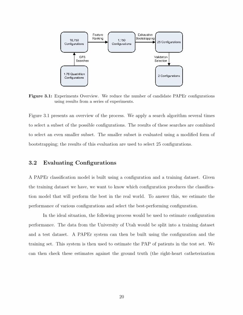
Figure 3.1: Experiments Overview. We reduce the number of candidate PAPEr configurationsusing results from a series of experiments.
Figure 3.1 presents an overview of the process. We apply a search algorithm several times
to select a subset of the possible configurations. The results of these searches are combined
to select an even smaller subset. The smaller subset is evaluated using a modified form of
bootstrapping; the results of this evaluation are used to select 25 configurations.
3.2 Evaluating Configurations
A PAPEr classification model is built using a configuration and a training dataset. Given
the training dataset we have, we want to know which configuration produces the classifica-
tion model that will perform the best in the real world. To answer this, we estimate the
performance of various configurations and select the best-performing configuration.
In the ideal situation, the following process would be used to estimate configuration
performance. The data from the University of Utah would be split into a training dataset
and a test dataset. A PAPEr system can then be built using the configuration and the
training set. This system is then used to estimate the PAP of patients in the test set. We
can then check these estimates against the ground truth (the right-heart catheterization
20

measurements made at the University of Utah) and calculate performance measures such as
sensitivity,1 specificity,2 and accuracy.3
Unfortunately it is very likely that the performance estimate is not very accurate.
The unreliability of the estimate is due to the limited amount of data used in the estimation
process. Because 31 of the 51 patients were held out as a validation set (more on this later)
our experiments were only able to use data from at most 20 patients. This forced training
and test sets to be very small.
Performance estimate unreliability can be intuitively understood by observing the
following. Classification models are inferred using a training dataset. If this dataset is small
then even a small change to it could alter the resulting model and thus its performance on
the test set. Also, if a randomly-chosen test dataset is small (say three patients in size) then
a model may, by chance, correctly estimate PAP for those three patients. This may be so
even if, on average, the model would only produce correct estimates for one in three patients
if it was operating in the real world. If a larger test dataset is used (30 or 100 patients) then
there is less chance of this happening.
Another way to look at this problem is to note that neither the training set nor the
test set is a representative sample of all patients. In statistics, a rule of thumb states that
a sample is not statistically significant until it includes at least 30 data points. Using this
rule of thumb we would like to have at least 60 patients, 30 for training and 30 for testing.
Even with the validation set we do not have this many patients.
Cross-validation and bootstrapping are two methods for addressing the small dataset
problem, although, as Isaksson (6) demonstrates, they are not ideal. The basic idea is to
repeat the performance estimation process (as described above) many times and then average
the results. Each repetition of the estimation process is done using a different split of the
dataset into train/test sets.
1Sensitivity is the percentage of sick patients that are classified correctly.2Specificity is the percentage of healthy patients that are classified correctly.3Accuracy is the percentage of all patients that are classified correctly.
21

Cross-validation and bootstrapping differ in the way that the dataset is split in each
iteration. Cross-validation “folds” the dataset into roughly equal-sized sets. One set is used
as the test set while the other sets are combined to form the training set. This is repeated,
with a different set being used as the test set, until all sets have been used as the test set
exactly once. Bootstrapping, on the other hand, creates a training set by randomly selecting
a given percent of the data; it creates a test using the rest of the data. This is repeated as
often as necessary.
The cross-validation method was used in the feature subset selection search (described
in Section 3.3). A variation on the bootstrapping approach was used in the configuration
selection experiments (described in Section 3.4).
3.3 Feature Subset Selection
The number of possible PAPEr configurations is huge. Five locations and five learning
algorithms can be used; also, any subset from the set of 46 considered features (except
the empty set) can be used. The number of possible subsets is 246 − 1, or roughly 70
trillion. Taking into account the 25 possible location/learner pairs, a total of about 1,759
trillion configurations are possible. We use a search algorithm to select a subset of these
configurations; evaluating them all is impractical.
There are many algorithms for doing feature subset selection, many of which are
described by Kohavi (8). Selection algorithms can be divided into filter algorithms and
wrapper algorithms. Filter algorithms analyze features (typically using statistical methods)
to determine the relevance of different feature subsets. Wrapper algorithms use the learner
to evaluate feature subsets. Since a learner will perform at different levels depending on
which feature subset is used as its input, the performance level can be used to score subsets.
So a wrapper algorithm searches through the space of possible feature subsets, determines
the resulting performance of the learner, and selects the feature subset that leads to the best
22

performance. Using the wrapper approach makes sense since the performance of PAPEr is
dependent on both the selected learning algorithm and the selected feature subset.
The feature subset selection algorithm we used can be described as a forward-selection
greedy search. Forward-selection simply means that a search begins with an empty set of
features; features are added to this set as the search progresses. This differs from the
backward-elimination approach which starts with all possible features and eliminates features
from the set during the search. The selection search is greedy because it iteratively adds the
single feature that will improve performance the most; it does not consider adding higher-
order sets of features.
3.3.1 Greedy Forward-Selection Search
We performed 25 greedy, forward-selection, feature subset selection searches, one search for
each of the location/learner pairs described in Chapter 2. We’ll refer to the searches as a
greedy forward-selection searches, or GFS searches.
Our GFS search starts with an empty list. One of the candidate features, F (see
Chapter 2 for the complete list of features), is then appended to the end of the list. At this
point a complete PAPEr configuration is defined by the location/learner pair and the feature
list (which is currently one feature long). This configuration is evaluated using the process
described in Section 3.2. Once evaluation is completed, F is removed from the end of the
list of features and another feature is appended. This again defines a configuration which is
evaluated. The process continues until all features have been added to (then removed from)
the list. Thus, all configurations that include just one feature are evaluated. The feature
associated with the best-performing configuration is permanently added to the list.
This whole process is repeated using all the candidate features except the feature
that was just added to the list. In this iteration of the search, the feature list includes the
previously-chosen feature plus one of the other features. The search finds the feature that,
23

combined with the previously-chosen feature, produces the best-performing configuration.
This new feature is then permanently added to the list.
The GFS search continues in this manner until a stopping criterion is met. One
possible criterion would stop the search when the best-performing configuration from the
current iteration of the search performs worse than the best-performing configuration from
the previous iteration. Our experiments did not use this criterion and instead simply ran the
search for 30 iterations. This is because we did not want the searches to end prematurely.
As can be seen in Figure 4.1, for some of the GFS searches the maximum performance value
occurred after the performance initially decreased.
3.3.2 Feature Ranking
The GFS searches produce 25 feature lists, each containing 30 features; this reduces the
number of considered feature subsets from 70 trillion to 750. We combine these results to
produce a single list of ranked features. The combined list of features contains all 46 features
described in Section 2.1; this further reduces the number of considered feature subsets to 46.
Using this single feature subset list also makes comparing locations and comparing learners
more straightforward.
We rank all 46 features by assigning a score to each feature. These scores are computed
using the 25 feature lists from the GFS searches. In effect this combines the 25 feature lists
into one list. The feature scoring is done using two assumptions about features in the 25
feature lists. We assume that features chosen early in a GFS search are more important than
features chosen later in the search. We also assume that features appearing in more of the
25 lists are more important than features appearing in fewer of the 25 lists. Remember that
each of the 25 lists contained 30 of the 46 features, so every feature did not appear in every
list. The following equation was used to score a feature: fscore =∑
l∈L 30 − f lrank, where
fscore is the feature score, L is the set of lists in which the feature appears, and f lrank is the
position in the list, l, at which the feature appears.
24

3.4 Exhaustive Bootstrapping
The list of ranked features was used to create 46 feature subsets. The first feature in the
list is the first subset; the first two features in the list become the second subset, and so
on until the 46th subset is created using all 46 features. Combined with the five locations
and five learners, we end up with 46× 5× 5 = 1150 configurations. We evaluate these 1150
configurations.
Using data from 20 patients, we use a modified version of bootstrapping (which we call
exhaustive bootstrapping) to evaluate the configurations. We repeatedly split the 20 patients
into training and test sets. Each split consisted of 18 patients in the training set and two
patients in the test set. Unlike normal bootstrapping where splits are formed randomly and
repeatedly a certain number of times, we systematically split the data in all possible ways
in which there are two patients in the test set. Splitting 20 patients in this way leads to 190
different splits, creating 190 different test sets each of size two. Each patient, X, appeared
in 19 of the test sets and was paired with a different patient, Y , each time. Consequently we
calculated 19 performance evaluations for each patient where each evaluation was associated
with a slightly-different training set.
Bootstrapping is used in an effort to mitigate the effects of working with a small
dataset and to reduce the variance in our performance estimate. It allows us to produce
more configuration evaluation results than cross validation. Exhaustive bootstrapping is used
instead of normal bootstrapping in order to ensure that there are no duplicate evaluation
results (two results originating from the same train and test sets). Exhaustive bootstrapping
also produces more performance estimates than a typical use of bootstrapping would, leading
to a decrease in the variance of our results.
We ended up with 190 test sets and 380 performance evaluations (each test set has
two patients in it) for each of the 1150 configurations. These 380 evaluations were averaged
to get an estimate of the classification accuracy of the configuration. Also, the 380 accuracy
25

measures were used to form a receiver-operator-characteristic (ROC) curve and from this to
calculate the area under the curve (AUC).
ROC curves plot the false-positive rate (FPR4) against the true-positive rate (TPR5)
as a given threshold changes. A PAPEr system classifies every heartbeat from a patient as
sick or healthy. If the percent of sick heartbeats from a patient crosses a set threshold then
the patient is classified as being sick. After setting the threshold to a certain level, a PAPEr
system can then produce classifications for all 380 “test” patients. From these classifications
we calculate the FPR and the TPR and then plot a point on the ROC graph. As we vary
the threshold, we continue plotting points until the ROC curve is fully plotted.
After evaluating all 1150 configurations we selected 25 of them (one for each loca-
tion/learner pair). This was done by choosing the feature subset that maximized the AUC.
3.5 Validation
We built 25 PAPEr systems using the 25 selected configurations. Each system was used to
classify the hold-out set of 31 patients. This was done by having each system classify all
heartbeats from each patient; a patient was classified as sick if the patient’s sick heartbeat
percentage crossed a calculated threshold.
Each of the 25 systems used a different threshold. The threshold was calculated using
its associated ROC curve. Remember that each point on the curve is associated with an
FPR, TPR, and a threshold. We want a low FPR and a high TPR so we assigned a score
to each threshold using the following equation: tscore = tTPR− tFPR, where tscore is the score
assigned to the threshold, tTPR is the TPR associated with the threshold, and tFPR is the
FPR associated with the threshold. Each system used the threshold that maximized tscore.
4FPR = FP/(FP + TN), where FP is the number of false-positives and TN is the number of true-negatives
5TPR = TP/(TP + FN), where TP is the number of true-positives and FN is the number of false-negatives
26

The results of classifying the hold-out set of 31 patients are presented in Section 4.5.
These results show that 2 of the 25 selected configurations clearly out-performed the others.
27
Chapter 4
Results
This chapter presents the results from the major experiments that were performed
for this thesis. It covers the 25 GFS searches, the ranked feature list, the 1,150 configuration
evaluations using exhaustive bootstrapping, the selection of 25 configurations from the set
of 1,150 configurations, and validation of the 25 selected configurations.
In this chapter several of the figures (and one of the tables) contain 25 graphs (25
cells in the case of the table) arranged in a 5-by-5 grid. To make it easier to refer to a specific
graph (or cell) within these figures (or the table) we will give them names. Each graph (cell)
corresponds to one of the 25 location/learner pairs. The first part of the name will indicate
the location (L1, L2, L3, L4, or L5) and the second part of the name will indicate the learner
(J48, KNN, MLP, NB, or SMO). So L1J48 refers to a graph associated with Location 1 and
the J48 learner.
4.1 GFS Search Results
Figure 4.1 shows results from the GFS searches (see Section 3.3.1). The values on the x-axis
of each graph indicate the size of the feature subset minus one—minus one because the graph
starts at zero instead of one. Each point on each graph corresponds to one configuration: a
location, a learner, and a feature subset. Each point has a y-axis value which is the estimated
accuracy of the configuration. This estimate was calculated using 10–fold cross validation
so the estimate is actually the average of 10 accuracies.
28

Figure 4.1: Greedy Forward-Selection Searches. The plots show the estimated accuracy of thePAPEr classification model as the 25 GFS searches progress. The plots contain 30points corresponding to the 30 feature subsets selected by each search.
Figure 4.1 does not show which features were contained in the various feature subsets.
Table 4.1 and Table 4.2 present this information. Each of the 25 GFS searches found 30
different feature subsets. The tables display 25 columns, one for each GFS search. Each
column is 30 rows in length, one row for each feature subset. A feature subset consists of
the feature in its row combined with all the features in the column in previous rows. For
instance, in Table 4.1 the first feature subset for the J48 learner using location 1 is {DA2S1}.
The second feature subset is {DA2S1 , R
QA2
QP2} The third feature subset is {DA2
S1 , RQA2
QP2, wS2}. This
pattern is followed for all 30 subsets.
A general pattern can be seen in the graphs in Figure 4.1. As the size of the feature
subset grows, the accuracy increases initially and then decreases. The amount of increase
and the amount of decrease varies from one location/learner pair to the next.
29

Learner J48 KNNLocation 1 2 3 4 5 1 2 3 4 5
1 DA2S1 sS4 iS4 QA2 QA2 cS2 iS4 iS4 iS3 iS3
2 RQP2
QA2HR SIS2 RQP2
QA2PS1 iS4 iS2 SIS2 SIS2 QS2
3 wS2 RPP2PA2
FP2 PS1 RQP2
QA2sS3 iS3 PP2 DP2
R SIS2
4 sS3 PS1 RFP2FA2
RPA2PS1
SIS2 RFP2FA2
PHB PS2 wS2 iS4
5 RFP2FA2
cS2 FA2 sS4 DA2R RQP2
QA2sS4 cS2 QP2 RPS2
PS1
6 iS4 DA2R DA2
R FA2 DP2R RPP2
PS2DA2
R sS3 DA2R PS2
7 RPS2PS1
DP2R sS3 SIS2 RPP2
PA2sS4 DA2
S1 PA2 RPS2PS1
RFP2FA2
8 RPP2PA2
DP2S1 RPP2
PS1iS4 iS4 wS2 RPP2
PS2PHB sS3 DA2
R
9 RPA2PS2
DA2S1 wS2 RPA2
PS2DP2
S1 iS3 DA2S1 FA2 RFP2
FA2DP2
R
10 cS1 iS4 FS2 RPP2PS2
DA2S1 RPP2
PS1DA2
R RPP2PA2
FA2 sS4
11 RPP2PS1
RFP2FA2
QHB iS1 RPA2PS1
SIS1 PA2 RPP2PS2
sS4 PHB
12 RPP2PS2
PHB RQP2
QA2wS2 sS4 FA2 PS2 sS4 QS2 QP2
13 RPA2PS1
PP2 QA2 DP2R PA2 RPP2
PA2PP2 wS1 cS2 RPA2
PS1
14 QP2 RPA2PS1
QS2 RPP2PA2
PS2 RPA2PS2
RPA2PS1
QA2 iS4 RPP2PA2
15 iS3 RPP2PS1
cS2 DA2R PP2 NSIS2 R
PP2PA2
RPP2PS1
DA2S1 FP2
16 QHB FP2 RPP2PA2
RPS2PS1
RPS2PS1
FS2 DP2S1 DP2
S1 RPP2PS1
DA2S1
17 FP2 PS2 QP2 RFP2FA2
RPP2PS1
DP2R DP2
R RPA2PS2
QHB DP2S1
18 NSIS1 RPS2PS1
SIS1 iS3 PHB PS2 RPP2PS1
wS2 FP2 PP2
19 cS2 PA2 DA2S1 wS1 wS2 DA2
R RPS2PS1
DA2S1 NSIS1 FA2
20 wS1 QA2 DP2R RPP2
PS1RFP2
FA2DA2
S1 QA2 iS3 SIS1 QA2
21 sS4 SIS2 FHB sS3 FA2 iS2 DP2R PS1 QA2 RQP2
QA2
22 iS2 QHB RPS2PS1
SIS1 iS1 FP2 cS2 DP2R RQP2
QA2NSIS2
23 SIS1 FHB sS4 FHB FP2 wS1 FA2 RPS2PS1
RPP2PS2
RPP2PS1
24 DA2R NSIS2 FS1 FP2 QP2 NSIS1NSIS2R
PA2PS1
DP2S1 FS2
25 FS2 FA2 RPP2PS2
QHB FS2 QA2 QS2 QS1 RPP2PA2
HR
26 NSIS2 RPA2PS2
NSIS1NSIS2 FS1 PP2 SIS1 RFP2FA2
NSIS2 RPP2PS2
27 PP2 FS1 RPA2PS2
FS1 QS2 QP2 FS2 DA2R PP2 wS1
28 FA2 SIS1 wS1 QP2 FHB DP2S1 SIS2 FP2 RPA2
PS1cS2
29 SIS2 DA2S1 QS1 QS2 sS3 PA2 sS3 SIS1 cS1 RPA2
PS2
30 QS2 NSIS1 cS1 QS1 QHB RPS2PS1
QP2 RQP2
QA2FS1 wS2
Table 4.1: Features Selected by the Greedy Forward-Selection Searches. Shown are the lists of30 features found by 10 of the 25 GFS searches. The features are listed in the orderin which they were selected by the GFS searches, as shown by the numbers in the leftcolumn.
30

Learner MLP NBLocation 1 2 3 4 5 1 2 3 4 5
1 SIS2 sS4 iS4 SIS2 PHB PS2 PHB sS4 PP2 iS2
2 RQP2
QA2HR SIS1 PHB QS2 FS2 PS1 RPP2
PS1QS1 RPA2
PS2
3 PA2 RPS2PS1
NSIS2 PA2 RQP2
QA2RQP2
QA2PP2 wS2 HR DP2
R
4 iS4 RPA2PS1
RPP2PS2
QA2 RPP2PA2
RPA2PS2
PS2 DP2R PS2 RPP2
PS2
5 iS3 RPP2PA2
DP2R RQP2
QA2FA2 RPP2
PS2iS4 DA2
R iS1 RPP2PA2
6 cS2 RPP2PS1
cS2 NSIS2 RFP2FA2
QP2 PA2 sS3 sS3 DA2R
7 RFP2FA2
cS2 DA2S1 RPA2
PS2QA2 RPP2
PA2cS1 RPP2
PA2RPA2
PS2DA2
S1
8 QA2 RPP2PS2
RPA2PS2
RFP2FA2
DA2R PA2 DP2
S1 QS2 wS2 DP2S1
9 RPP2PA2
DA2R DA2
R sS4 DP2R RFP2
FA2RPP2
PA2QP2 PA2 RQP2
QA2
10 RPA2PS2
DP2R RPP2
PS1iS3 RPP2
PS2iS4 DA2
S1 RPA2PS2
sS4 sS3
11 DA2S1 PP2 RFP2
FA2wS1 FP2 FP2 sS4 PA2 FP2 QP2
12 iS2 DP2S1 RPP2
PA2PS1 RPA2
PS1QS1 iS2 QS1 FS2 cS2
13 DP2S1 iS1 DP2
S1 wS2 PP2 SIS1 QS2 DA2S1 wS1 PA2
14 cS1 cS1 RPA2PS1
cS2 PS2 QS2 DP2R QA2 QS2 PS2
15 wS2 PS2 iS3 sS3 HR wS1 iS1 cS1 FS1 RFP2FA2
16 FA2 RPA2PS2
QA2 FA2 SIS2 sS4 DA2R RPP2
PS2RPP2
PS2SIS2
17 RPP2PS2
DP2S1 RPS2
PS1PP2 iS2 sS3 QS1 FP2 QHB wS2
18 sS3 PHB FP2 RPP2PA2
cS1 iS3 SIS2 cS2 QP2 QS1
19 wS1 DA2R FA2 FP2 NSIS2 wS2 sS3 FA2 RFP2
FA2sS4
20 QP2 DA2S1 RQP2
QA2PS2 RPS2
PS1cS1 RPA2
PS2RPS2
PS1RQP2
QA2QA2
21 QS2 PA2 DA2S1 RPP2
PS2RPP2
PS1QHB QA2 DP2
S1 NSIS2 PP2
22 RPA2PS1
DA2S1 PS1 FS2 FS2 FHB NSIS2 FS2 QA2 QS2
23 sS4 PS1 PA2 QS2 RPA2PS2
PP2 RPP2PS2
SIS2 SIS1 cS1
24 NSIS2 FA2 cS1 HR PA2 cS2 QP2 FHB RPP2PA2
wS1
25 FP2 FP2 SIS2 QP2 cS2 RPS2PS1
FP2 RPA2PS1
FA2 FA2
26 DA2S1 QA2 PS2 NSIS1 sS4 RPP2
PS1FS1 iS2 cS2 iS4
27 DP2S1 iS3 DP2
S1 iS2 iS4 NSIS1 RPA2PS1
QHBNSIS1 FS2
28 PHB SIS2 wS1 QS1 DP2S1 RPA2
PS1FA2 FS1 DA2
R NSIS2
29 RPP2PS1
FS2 NSIS1 iS1 DA2S1 NSIS2 cS2 RQP2
QA2PHB iS3
30 SIS1 iS4 PP2 DA2R DP2
S1 QA2 FS2 PHB SIS2 FS1
Table 4.2: Features Selected by the Greedy Forward-Selection Searches. Shown are the lists of30 features found by 10 of the 25 GFS searches. The features are listed in the orderin which they were selected by the GFS searches, as shown by the numbers in the leftcolumn.
31

Learner SMOLocation 1 2 3 4 5
1 iS1 iS1 iS1 iS1 iS1
2 QHB QA2 FHB QS1 QS1
3 RPA2PS2
FA2 RFP2FA2
FS1 iS4
4 cS1 RPP2PA2
RQP2
QA2QP2 RPP2
PA2
5 RPP2PA2
PA2 DA2R RQP2
QA2DP2
R
6 RFP2FA2
PHB DP2R RFP2
FA2DA2
R
7 iS4 PS2 FP2 RPP2PS2
FHB
8 wS2 PP2 QA2 FA2 RFP2FA2
9 sS4 DA2R RPA2
PS1FP2 SIS2
10 RQP2
QA2FHB cS2 sS3 sS4
11 iS3 RPA2PS1
RPP2PA2
QHB sS3
12 QA2 DP2R QS1 sS4 DP2
S1
13 FA2 DP2S1 DA2
S1 RPP2PA2
DA2S1
14 RPP2PS2
DA2S1 PS2 NSIS2 FP2
15 cS2 QHB QS2 PHB QP2
16 wS1 PS1 QP2 SIS1 QA2
17 FHB cS1 PA2 FHB QHB
18 DP2S1 SIS2 wS2 RPA2
PS2wS2
19 sS3 RPS2PS1
sS4 iS2 FS2
20 NSIS1 RPP2PS1
cS1 FS2 RQP2
QA2
21 QS2 SIS1 DP2S1 cS1 FA2
22 QP2 sS3 RPP2PS2
SIS2 RPA2PS1
23 SIS1 NSIS2 sS3 wS2 NSIS2
24 DP2R QP2 SIS1 QA2 RPS2
PS1
25 NSIS2 DP2S1 RPP2
PS1iS3 RPP2
PS1
26 RPA2PS1
FS2 NSIS1 DP2S1 cS1
27 DA2S1 RFP2
FA2RPS2
PS1PP2 RPA2
PS2
28 RPP2PS1
FS1 FS1 cS2 iS3
29 RPS2PS1
QS2 RPA2PS2
wS1 RPP2PS2
30 DA2S1 FP2 FA2 NSIS1 PP2
Table 4.3: Features Selected by the Greedy Forward-Selection Searches. Shown are the lists of30 features found by 5 of the 25 GFS searches. The features are listed in the order inwhich they were selected by the GFS searches, as shown by the numbers in the leftcolumn.
32

4.2 Ranked Feature List
Table 4.1 and Table 4.2 were combined to create a ranked feature list (see Section 3.3.2).
The ranked feature list is shown in Table 4.4. The features are ranked in descending order
from most important to least important feature.
We expected that features extracted from the S2 sound would be helpful in classifying
a patient. On the other hand we expected that other features, such as those extracted from
the S1 sound or the whole heartbeat sound, would be less helpful. The ranked feature list
confirmed these expectations, although some exceptions did occur.
The features extracted from the whole heartbeat sound were not very helpful. FHB,
QHB, PHB, and HR are all ranked in the second half of the list. The features wholly-
dependent on the S1 sound (iS1, cS1, QS1, PS1, SIS1, wS1, FS1) were also all ranked in
the second half of the list. Together, these features make up 11 of the 23 features in the
second-half of the list.
The ventricular systole duration estimates (DA2S1 , DP2
S1 , DA2R , and DP2
R ) were not pre-
dictive, as indicated by their ranking in the ranked feature list. They occupied the 41st
ranking and the last three rankings. However, simply dividing these duration times by the
whole heartbeat time increased the predictivity. The features DA2R , DP2
R , DA2S1 , and DP2
S1
occupy the 5th, 7th, 16th, and 25th rankings. Thus, the percentage of the heartbeat taken for
ventricular systole was much more predictive than the absolute duration time of ventricular
systole.
In Section 2.1.3 we mentioned that Chen found little statistical correlation between
PAP and FA2, QA2, and RQP2
QA2(4). The ranked feature list gives these features more credit,
ranking them, respectively, at 13th, 8th, and 6th.
Feedback from Dr. Michaels confirms that many of the features in the ranked feature
list are ranked in accordance with his expectations based on his medical knowledge. The RPP2PA2
feature is “felt to be a powerful predictive bedside tool to diagnose pulmonary hypertension”
(10). He also expected SIS2 to be a useful feature. “Heart rate, systolic ejection period,
33

Rank 1 2 3 4 5 6 7 8 9 10
Feature RPP2PA2
sS4 RFP2FA2
iS4 DA2R RQP2
QA2DP2
R QA2 RPP2PS2
SIS2
Rank 11 12 13 14 15 16 17 18 19 20
Feature sS3 RPA2PS2
FA2 cS2 wS2 DA2S1 PS2 PA2 FP2 RPP2
PS1
Rank 21 22 23 24 25 26 27 28 29 30
Feature QP2 RPA2PS1
PP2 iS3 DP2S1 PHB RPS2
PS1iS1 QS2 cS1
Rank 31 32 33 34 35 36 37 38 39 40Feature NSIS2 QS1 PS1 QHB FS2 SIS1 iS2 wS1 FHB HRRank 41 42 43 44 45 46
Feature DA2S1 FS1 NSIS1 DP2
S1 DA2R DP2
R
Table 4.4: Ranked Feature List. This list of ranked features was produced by combining thefeature lists from the 25 GFS searches.
S1 splitting, are not useful”, which is reflected in the ranked feature list (10). He expected
one set of features, those that measure “heart sound resonance” (the Q-factor features), to
have “some predictive value, but the data shows it is not predictive” (10). QA2 was the only
Q-factor feature with good predictive value.
4.3 Configuration Evaluations
Figure 4.2 shows the result of evaluating 1150 different configurations (see Section 3.4). In
comparing configurations we decided to use the AUC measurement instead of the accuracy
measurement. This is because the AUC measurement is more sensitive to how well the
configuration is able to separate the healthy and sick patients into distinct groups. This can
be seen in Figure 4.2. The red lines (AUC) are more volatile than the blue lines (accuracy).
Configurations with the same accuracy can have very different AUC measurements.
A configuration for each location/learner pair was selected. The red dots in Figure
4.2 indicate these configurations. The size of the feature subsets in most of these selected
configurations ranged between 10 and 30. From the perspective of trying to optimize PAPEr
this is no problem. However, from a medical perspective having 10 to 30 features makes it
difficult to try to explain why these features are useful in estimating PAP. Future work could
address this problem.
34

Figure 4.2: Exhaustive Bootstrapping Results. The configurations evaluated consisted of all com-binations of locations (5), learners (5), and feature subsets from the ranked featurelist (46) for a total of 5 × 5 × 46 = 1, 150 configurations. Each configuration wasevaluated using 190 different test sets. The blue line shows the average accuracy andthe red line shows the AUC. The red dot in each graph indicates the configurationwith the highest AUC.
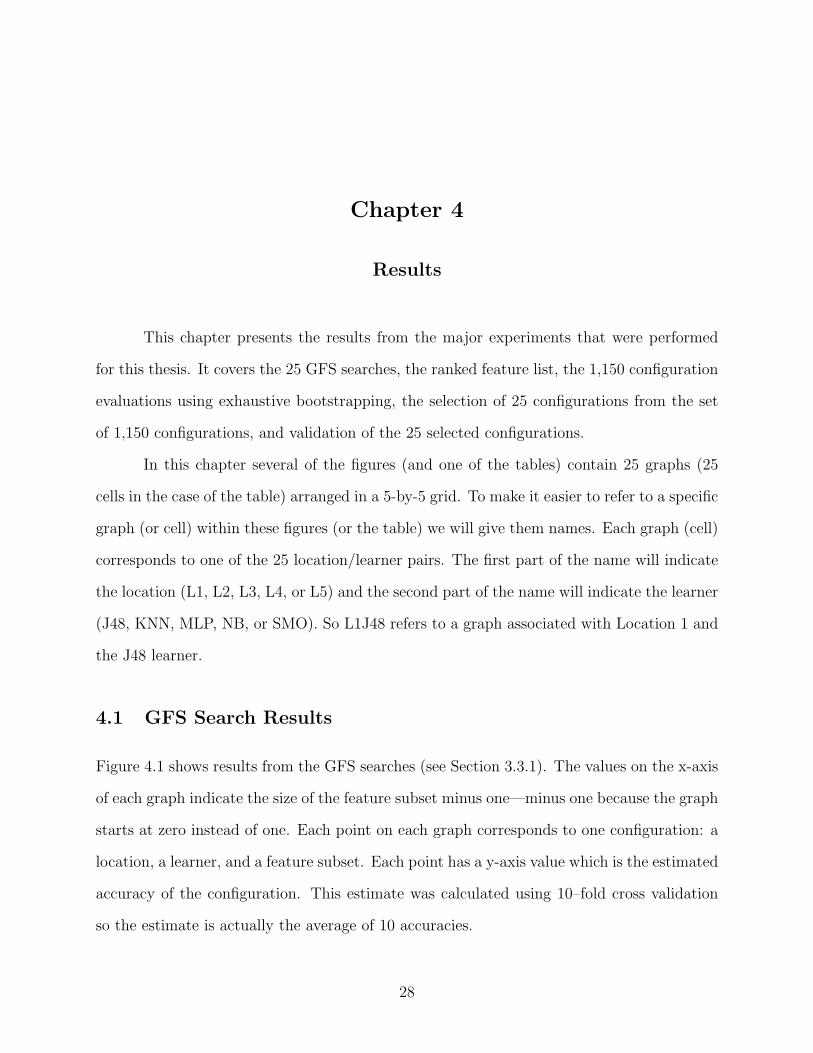
The graphs in Figure 4.3 show the ROC curves for the 25 selected configurations from
Figure 4.2. The chosen threshold value is displayed in the lower-right corner of each graph.
Each red dot in the graphs in Figure 4.3 shows the point on the ROC curve associated with
the selected threshold. This point indicates the estimated real-world true-positive rate and
false-positive rate that we expect from the configuration when using the indicated threshold.
For example, the point on the ROC curve from the L5NB graph indicates an 80 percent
true-positive rate and a 10 percent false-positive rate.
4.4 Overall Performance
We have used an “argmax” approach to select the best configuration: whichever configuration
performs the best is chosen. Another approach is to select a particular location, then a
particular learner, then a particular feature subset. Location selection could be done by
35
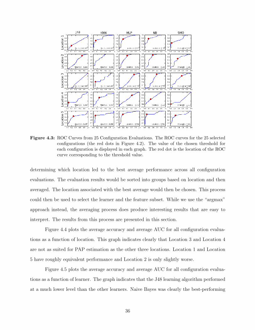
Figure 4.3: ROC Curves from 25 Configuration Evaluations. The ROC curves for the 25 selectedconfigurations (the red dots in Figure 4.2). The value of the chosen threshold foreach configuration is displayed in each graph. The red dot is the location of the ROCcurve corresponding to the threshold value.
determining which location led to the best average performance across all configuration
evaluations. The evaluation results would be sorted into groups based on location and then
averaged. The location associated with the best average would then be chosen. This process
could then be used to select the learner and the feature subset. While we use the “argmax”
approach instead, the averaging process does produce interesting results that are easy to
interpret. The results from this process are presented in this section.
Figure 4.4 plots the average accuracy and average AUC for all configuration evalua-
tions as a function of location. This graph indicates clearly that Location 3 and Location 4
are not as suited for PAP estimation as the other three locations. Location 1 and Location
5 have roughly equivalent performance and Location 2 is only slightly worse.
Figure 4.5 plots the average accuracy and average AUC for all configuration evalua-
tions as a function of learner. The graph indicates that the J48 learning algorithm performed
at a much lower level than the other learners. Naive Bayes was clearly the best-performing
36

Figure 4.4: Location Performance. Results from the experiments described in Section 4.3 aregrouped based on location. The average accuracy (blue line) and average AUC values(red line) are plotted here.
learner. KNN and MLP performed at about the same level. SMO’s accuracy was comparable
to KNN and MLP but its average AUC measure was significantly worse.
Figure 4.6 plots the average accuracy and average AUC for all configuration evalua-
tions as a function of feature subset. The same trend is seen in this graph that is generally
seen in Figure 4.1. As the size of the feature subset grows, the performance initially increases
quickly and then gradually decreases.
It is interesting to note which features, when added to the feature subset, caused
a significant increase in performance. The first major increase happened when sS4 was
added. The second increase is due to adding iS4. This is somewhat unexpected since both
of these features are S4 features and not the S2 features that we expected to be most useful.
However, Dr. Michaels notes that the presence of an S3 and/or S4 sound is “useful in
assessing pulmonary hypertension” (10).
The third major increase in performance occurred when SIS2 was added to the feature
subset. We expected this feature to be useful in PAP estimation because of its being studied
37

Figure 4.5: Learner Performance. Results from the experiments described in Section 4.3 aregrouped based on learner. The average accuracy (blue line) and average AUC values(red line) are plotted here.
and found useful in several medical papers. The fact that it initiated a large a jump in
performance is further evidence to its usefulness in PAP estimation.
Three more minor increases in performance were initiated by the addition of cS2, wS2,
and PS2. Each of these is a feature of the S2 heart sound alone. This supports the hypothesis
that features of the S2 heart sound are useful in PAP estimation.
4.5 Holdout Set Classification
Tables 4.5 and 4.6 show results from the validation experiments (see Section 3.5). In these
experiments we classified the 31 hold-out patients using the 25 selected configurations. The
sensitivity, specificity, accuracy, and AUC are shown for each configuration. These numbers
estimate the real-world performance of each configuration and we analyze them to select the
best-performing configurations.
PAPEr could be used as a screening test to determine the need for further tests, such
as right-heart catheterization. In this scenario it is important that PAPEr have high sensi-
38

Figure 4.6: Feature Performance. Results from the experiments described in Section 4.3 aregrouped based on feature subset. The average accuracy (blue line) and average AUCvalues (red line) are plotted here.
J48 KNN MLP NB SMOLocation 1 56/54 89/15 56/77 72/85 56/77Location 2 17/100 33/100 44/77 33/85 39/85Location 3 0/100 0/100 22/85 17/85 39/92Location 4 94/0 6/85 44/77 72/62 94/23Location 5 56/54 0/100 72/54 78/46 78/69
Table 4.5: Validation Results: Sensitivity and Specificity. We classified 31 patients (the hold-outset) using each of the 25 selected configurations. The sensitivity (number on the left)and specificity (number on the right) are shown for each configuration.
tivity because classifying a sick patient as healthy is very costly. If such a misclassification
is produced then the patient will not receive needed treatment. On the other hand PAPEr
could also be used as a confirmatory test, in which case it is important that PAPEr have
high specificity. A configuration can be tuned for one test or the other by raising or lowering
its decision threshold, though this does involves a tradeoff. Increasing the sensitivity of a
configuration will decrease its specificity and vice versa.
The accuracy and AUC1 measurements, shown in Table 4.6, account for both sensi-
tivity and specificity; consequently, the accuracy and AUC measurements are less dependent
on the choice of threshold. We use these measurements to select the best configuration. It
is obvious from looking at Table 4.6 that L1NB is the best configuration. The performance
of L5SMO is only a little worse than L1NB.
1Results from the validation experiments do not allow us to directly calculate AUC values. The AUCvalues given in Table 4.6 are estimated using the equation AUC = (sensitivity + specificity)/2.
39
J48 KNN MLP NB SMOLocation 1 55/55 58/52 65/66 77/78 65/66Location 2 52/58 61/67 58/61 55/59 58/62Location 3 42/50 42/50 48/53 45/51 61/66Location 4 55/47 39/45 58/61 68/67 65/59Location 5 55/55 42/50 65/63 65/62 74/74
Table 4.6: Validation Results: Accuracy and AUC. We classified 31 patients (the hold-out set)using each of the 25 selected configurations. The accuracy (number on the left) andAUC (number on the right) are shown for each configuration. The AUC values havebeen multiplied by 100 to make them easier to read.
The selection of L1NB and L5SMO is somewhat surprising given the results presented
in Figure 4.2. The results in this figure suggest that L5NB would perform very well and
that L5SMO would not be among the best configurations. The validation experiment results
show L5NB doing worse than expected and L5SMO doing better than expected.
One possible reason for the success of L1NB and L5SMO is that both used learning
algorithms that avoid overfitting the training data. Overfitting is a particular challenge
when the training data is sparse, which is the case in our experiments. The naive Bayes
algorithm and SMO algorithm avoid overfitting by producing simple decision surfaces (a
linear SVM was used in L5SMO) that are unable to conform too closely to the training data.
For example, the decision surface used by L5SMO is a hyperplane that cuts through the
input feature space.
The performance of L1NB and L5SMO is very promising. They are both close to
being real-world ready. Both configurations meet the goal given to us by Dr. Michaels of
achieving 0.7 or greater AUC (see Section 1.2).
A PAPEr system built using L1NB, L5SMO, or one of the other configurations would,
of course, need further testing and verification before enough confidence could be placed in
the system to use it in real-world situations. This is another consequence of not having
enough data in our datasets. However, our results give us confidence that a dependable
PAPEr system can be built.
40

Chapter 5
Conclusion
The goal of this thesis was to develop a system, called PAPEr, to estimate PAP
noninvasively. A fully-developed system to do this would help lower diagnostic costs by
replacing the use of right-heart catheterization in some patients.
We experimented with heart sound analysis as a technique for producing PAP es-
timates. Several papers in the medical research literature suggest that this is a promising
technique, especially the analysis of the S2 heart sound. In this thesis we used the tools of
machine learning to perform the heart sound analysis.
Developing PAPEr involved running several experiments. These experiments were
geared toward answering three questions. What chest wall location should we use in recording
the heart sounds? What learning algorithm should be used to produce the PAP estimates?
What set of heart sound features should be used as input to the learning algorithm? The
experiments resulted in several promising potential configurations of the PAPEr system.
We did not focus much effort on calculating high-quality feature values from the heart
sounds. Typically the quickest and easiest method was used. In particular, our method of
calculating SIS2 is not as advanced as the methods described in (18) and (19). Incorpo-
rating these methods into PAPEr could lead to better SIS2 values and, presumably, better
performance. This is true of the other heart sound features as well.
We made little effort to throw away features that could be considered noisy. We
did not hand-pick the heartbeats we used in the datasets. Instead, we trusted the machine
learning algorithms to perform well despite the noisy data. We made this decision partly
41

based on the results of some preliminary experiments (see Section 2.1.2). However, these
results were not decisive in showing that removing noise could not help improve performance.
It is quite possible that some form of noise removal could improve performance of a future
PAPEr system.
The larger point here is that we spent little time and effort on performing preprocess-
ing of any kind—noise removal included. On the one hand, the fact that PAPEr performs
as well as it does without any special tweaking speaks to its robustness. On the other hand,
various preprocessing steps could potentially improve PAPEr’s performance and reliability.
The promising configurations found in this thesis all use somewhat large feature
subsets. At least the feature subsets are large in the context of trying to interpret why the
features are helpful in estimating PAP, which is very important to the medical community.
Finding a smaller feature subset that still produces good performance is an important goal
for future work. One approach is to perform a backward-elimination search on the selected
feature subsets.
Decreasing the size of the selected feature subset used in PAPEr would aid the devel-
opment of a physiological theory for how and why PAPEr works. It would increase PAPEr’s
interpretability. A physiological theory could lead to new or better insights into how the
heart-lung system works. The theory could also increase PAPEr’s acceptance in the medical
community, further justify the development of PAPEr as part of a medical device, and help
doctors in practice adopt PAPEr as a valuable tool.
Currently, our system makes a very imprecise estimate of PAP; it simply reports
whether the PAP is above or below a certain threshold, where the threshold is the pressure
above which a patient is considered to have pulmonary hypertension. It would be useful for
future systems to produce an actual PAP value instead. This would provide doctors with
valuable information about the severity of a patient’s pulmonary hypertension or about the
likelihood of a patient developing pulmonary hypertension.
42

As a quick attempt at implementing a PAPEr system that produces PAP values,
we trained an L5MLP configuration using PAP values instead of pulmonary hypertension
diagnoses. We measured the performance of L5MLP using the standard error of estimate
(SEE1). On the hold-out set of 31 patients it has an SEE of 11.7 mmHg. On the training set
(the group of 20 patients) it has an SEE of 5.1 mmHg. This compares favorably with the
results reported in (19); the SEE for the humans in that study is 5.8 mmHg. These results
indicate that one focus of future work should be the development of a reliable and accurate
PAPEr system that produces PAP values.
The PAPEr configurations in this thesis need to undergo more testing before being
used in the real world. This will require more patient data. Having more training data to
train the classifiers would potentially lead to better classifiers. And testing the configurations
on larger test sets is needed. This is critical for calculating more reliable and more accurate
performance estimates. The larger the pool of validation patient data, the more confident
we can be in the performance estimates.
We asked Dr. Michaels for his thoughts on the PAPEr system. “From a cardiol-
ogy perspective, this work is extremely interesting. It reinforces useful clinical tools, and
identifies computerized tests (not available with the stethoscope alone) that may increase
the diagnostic accuracy for pulmonary hypertension...I think this work is innovative, and
provides a nice framework for the acoustic evaluation of pulmonary hypertension” (10).
1SEE =√∑
(PAPest − PAPact)2/(N − 2), where PAPest is the estimated PAP value, PAPact is theactual PAP value, and N is the number of estimate/actual PAP value pairs.
43
References
[1] S. Aggio, E. Baracca, C. Longhini, C. Brunazzi, L. Longhini, G. Musacci, and
C. Fersini, “Noninvasive estimation of the pulmonary systolic pressure from the spectral
analysis of the second heart sound,” Acta Cardiologica, vol. 45, no. 3, pp. 199–202, 1990,
PMID: 2368539. [Online]. Available: http://www.ncbi.nlm.nih.gov/pubmed/2368539
[2] D. W. Aha, D. Kibler, and M. K. Albert, “Instance-based learning algorithms,”
Machine Learning, vol. 6, no. 1, pp. 37–66, 1991. [Online]. Available: http:
//dx.doi.org/10.1007/BF00153759
[3] C. J. C. Burges, “A tutorial on support vector machines for pattern recognition,” Data
Mining and Knowledge Discovery, vol. 2, no. 2, pp. 121–167, 1998.
[4] D. Chen, P. Pibarot, G. Honos, and L. Durand, “Estimation of pulmonary
artery pressure by spectral analysis of the second heart sound,” The Amer-
ican Journal of Cardiology, vol. 78, no. 7, pp. 785–789, Oct. 1996.
[Online]. Available: http://www.sciencedirect.com.erl.lib.byu.edu/science/article/
B6T10-3P69WM6-1C/2/1b427020903b04a2a9ee8cca1396fddb
[5] E. Coiera, Guide to health informatics, 2nd ed. London: Arnold, 2003.
[6] A. Isaksson, M. Wallman, H. Goransson, and M. G. Gustafsson, “Cross-validation and
bootstrapping are unreliable in small sample classification,” Pattern Recognition Letters,
vol. 29, no. 14, pp. 1960–1965, 2008.
[7] G. John and P. Langley, “Estimating continuous distributions in Bayesian classifiers,” in
Proceedings of the Eleventh Conference on Uncertainty in Artificial Intelligence. Mor-
gan Kaufmann, 1995, pp. 338–345.
[8] R. Kohavi and G. H. John, “Wrappers for feature subset selection,” Artificial Intelli-
gence, vol. 97, no. 1-2, pp. 273–324, 1997.
[9] I. Kononenko, “Machine learning for medical diagnosis: history, state of the
art and perspective,” Artificial Intelligence in Medicine, vol. 23, no. 1, pp.
44

89 – 109, 2001. [Online]. Available: http://www.sciencedirect.com/science/article/
B6T4K-43HBR8T-7/2/c9823c01306f06fb2ced5ea83e62baa5
[10] A. Michaels, private communication, 2009.
[11] T. M. Mitchell, Machine Learning. New York: McGraw-Hill, 1997.
[12] J. C. Platt, “Fast training of support vector machines using sequential minimal
optimization,” in Advances in Kernel Methods: Support Vector Learning. MIT
Press, 1999, pp. 185–208. [Online]. Available: http://portal.acm.org/citation.cfm?id=
299105&dl=
[13] J. R. Quinlan, C4.5: programs for machine learning. Morgan Kaufmann Publishers
Inc., 1993. [Online]. Available: http://portal.acm.org/citation.cfm?id=152181
[14] P. Sajda, “Machine learning for detection and diagnosis of disease,” Annual Review
of Biomedical Engineering, vol. 8, pp. 537–565, 2006, PMID: 16834566. [Online].
Available: http://www.ncbi.nlm.nih.gov/pubmed/16834566
[15] M. C. Staff, “Pulmonary hypertension,” http://www.mayoclinic.com/health/
pulmonary-hypertension/DS00430, Feb. 2008.
[16] C. Tranulis, L. Durand, L. Senhadji, and P. Pibarot, “Estimation of pulmonary
arterial pressure by a neural network analysis using features based on time-frequency
representations of the second heart sound,” Medical and Biological Engineering
and Computing, vol. 40, no. 2, pp. 205–212, Mar. 2002. [Online]. Available:
http://dx.doi.org/10.1007/BF02348126
[17] I. H. Witten and E. Frank, Data Mining: Practical machine learning tools and tech-
niques, 2nd ed. San Francisco: Morgan Kaufmann, 2005.
[18] J. Xu, L. Durand, and P. Pibarot, “Extraction of the aortic and pulmonary compo-
nents of the second heart sound using a nonlinear transient chirp signal model,” IEEE
Transactions on Biomedical Engineering, vol. 48, no. 3, pp. 277–283, March 2001.
[19] ——, “A new, simple, and accurate method for non-invasive estimation of pulmonary
arterial pressure,” Heart (British Cardiac Society), vol. 88, no. 1, pp. 76–80, Jul. 2002,
PMID: 12067952. [Online]. Available: http://www.ncbi.nlm.nih.gov/pubmed/12067952
45