NONLINEAR ANALYSIS OF PLANE FRAMES USING A COROTATIONAL

FOMULATION AND PLASTICITY BY LAYERS IN A TIMOSHENKO BEAM EL-

EMENT

Sebastião Simão da Silva , William Taylor Matias Silva

Department of Civil and Environmental Engineering, Postgraduate Program in Structure and

Civil Construction Engineering, University of Brasília (sebastiaosim@unb.br)

Abstract. The purpose of this work is to perform a nonlinear analysis of plane frame struc-

ture using a corotational formulation and a layered plastic modeling. The plane frame is dis-

cretized with a 2D Timoshenko beam element. Plasticity is introduced by rate-independent

Von-Mises model with isotropic hardening. Numerical integration over the cross-section is

performed for obtain the internal force vector and tangent stiffness matrix of these elements.

At each integration point, the backward-Euler algorithm is used for integration in the consti-

tutive equations. Some examples are used in order to check the performances in the elements

and the path-following procedures.

Keywords: Nonlinear analysis of structures; Corotational formulation; Plasticity in layers;

Finite element method.

1. INTRODUCTION

The linear analysis presents difficulties for analysis the real behavior of unusual struc-

tures, when the loading conditions is not common, or in structures close to collapse. In this

context, the nonlinear material and geometric has wide applicability in structural engineering.

In the geometric nonlinear analysis using finite element method, three different types of

kinematic descriptions have been widely used: total lagrangian description, updated lagrangi-

an description and corotacional description [10]. The latter is originates from the polar de-

composition theorem which states that the total deformation of a solid surface can be decom-

posed into rigid body motion and relative deformation [6] – Figure 1.

The concept of kinematic description corotacional was introduced in a context FEM in

the 60s of last century with the work of Argyris [1], is the latest of the formulations used in

geometrically nonlinear analysis and has a wide variety of subjects to be investigated [5].

Blucher Mechanical Engineering ProceedingsMay 2014, vol. 1 , num. 1www.proceedings.blucher.com.br/evento/10wccm

Figure 1. Kinematic description of the corotacional formulation.

When the answer in the solid structure is elastic, ceased loading, the body does not ex-

hibit deformation. However, when the answer is plastic after ceased the loading the material

shows residual strain [7][8]. The theory of plasticity provides laws and models capable of

describing the constitutive behavior of materials with elastoplastic response.

2. METHODOLOGY APPROACH

In this work used a 2D Timoshenko beam element (C0) without coupling of the axial and

bending effort. To perform numerical simulations with the described formulation, implement

in the finite element program 2D_Beam_f90 the beam elements mentioned above using the

corotational formulation. In the treatment of plasticity has been used a layered unidimensional

bilinear model with isotropic hardening. Integrates this model using an implicit algorithm

named backward-Euler [11]. For the sectional efforts, integrate normal stresses using seven or

fifteen Gauss points along the depth of the cross section. Vector of internal forces and tangent

stiffness matrix of element mentioned above was determined through the principle of virtual

work. The coefficients of these vectors and matrices were obtained by numerical integration.

For the trajectory equilibrium nonlinear adopts an analysis based on the iterative incremental

Newton-Raphson method and arc length technique.

3. COROTATIONAL FORMULATION OF PLANES FRAMES

The formulation described here is presented in Battini [2], which differs slightly from

the other one shown in Crisfield [3].

3.1 Kinematic description of a beam element

In Fig 1 shows the coordinates of the nodes 1 and 2 in the global coordinate system

,x z - 1 1,x z and 2 2,x z , respectively (Figure 2). The global displacement vector is defined

by:

gu 1 1 1 2 2 2

Tu w u w . (1)

Figure 2. Corotacional Fomulation – beam kinematics.

Furthermore, the local displacement vector is given by:

l

u 1 2 T

u . (2)

The l

u components can be calculated by the following equations,

0nu l l , 1 1 and 2 2 . (3)

In the equations above 0l and

nl denote the initial and current lengths, respectively. Us-

ing simple trigonometric relationships the lengths may be rewritten as:

1

2 2 2

0 2 1 2 1l x x z z

and 1

2 2 2

2 2 1 1 2 2 1 1nl x u x u z w z w

(4)

where denotes the rigid body rotation. This may be related trigonometrically by

0 0sen c s s c and

0 0cos c c s s , (5)

which, after developed, leads:

0 0 2 1

0

1cosc x x

l , 0 0 2 1

0

1s sen z z

l ,

2 2 1 1

1cos

n

c x u x ul

and 2 2 1 1

1

n

s sen z w z wl

. (6)

Thus, for , is given by:

1sen sen if 0sen and cos 0 ; 1cos cos if 0sen and cos 0

1sen sen if 0sen and cos 0 and 1cos cos if 0sen and cos 0 (7)

3.1.1 Virtual displacements

Deriving the equation (3) obtains the virtual local displacements,

2 1 2 1 0 0u c u u s w w c s c s gu , (8)

1 1 1 0 and (9)

2 2 2 . (10)

On the other hand, can be calculated by differentiation of Equation (6d)

2 1 2 2 1 12

1n n

n

w w l z w z w lcl

, (11)

where nl u is given by Equation (8). Using Eq (6d), the expression becomes

2

2 1 2 1 2 1

1n

n

w w l sc u u s w wcl

, (12)

which, after simplifications produces

1

0 0n

c s c sl

gu . (13)

Thus, the transformation matrix B is defined as

l

u B ug , (14)

and given by,

0 0

1 0

0 1

n n n n

n n n n

c s c s

s l c l s l c l

s l c l s l c l

B . (15)

3.1.2 Internal force vector

The relationship between the internal local force vector l

f and global g

f is obtained by

the equation of virtual work in local and global systems

T T T T

g g l l g lV u f u f u B f (16)

Equation (16) must be applied to any gu arbitrary. Thus, the global internal force vec-

tor is given by

T

g lf B f (17)

in which the local internal force vector T

l 1 2N M Mf depends on the definition of the

finite element beam specific employed.

3.1.3 Tangent stiffness matrix

The global tangent stiffness matrix gK defined by

g g g f K u (18)

is obtained by variation of Equation (17). Thus,

T

g l 1 1 2 2 3N b M b M b f B f . (19)

In the above equation 2b is, for example, the second column of

TB . The following no-

tations are introduced,

0 0T

c s c s r and 0 0T

s c s c z (21)

which by differentiation become,

r z and z r . (22)

The equation (8) and (13) may be rewritten as

T

n gu l r u and

1 T

g

nl

z u . (23)

Introduces auxiliary expressions,

1 b r , 2

10 0 1 0 0 0

T

nl

b z and 3

10 0 0 0 0 1

nl

T

b z (24)

derivatives produce,

1

T

g

nl

zz

b r p and 2 3

1 T Tng2 2

n n n

l

l l l

zzb b rz zr p . (25)

The first term in Eq (19) is calculated by the introduction of the local tangent stiffness

matrix lK , which depends on the element definition.

l l l l g f K u K B u (26)

Finally, from Equation (18), (19), (25a), (25b) and (26), the expression of the global

stiffness matrix tangent becomes

2

1

n

T T T T

g l 1 2

n

NM M

l l K B K B zz rz zr (27)

The equation (14) and (27) provide the connection between the internal forces and stiff-

ness matrices tangent local and global. These relationships are independent of the local defini-

tion of the element. This is obtained by adopting assumptions: Bernoulli deformation, linear

elastic constitutive relation, the principle of virtual work (PTV) -

1 1 2 2v

V dv N u M M .

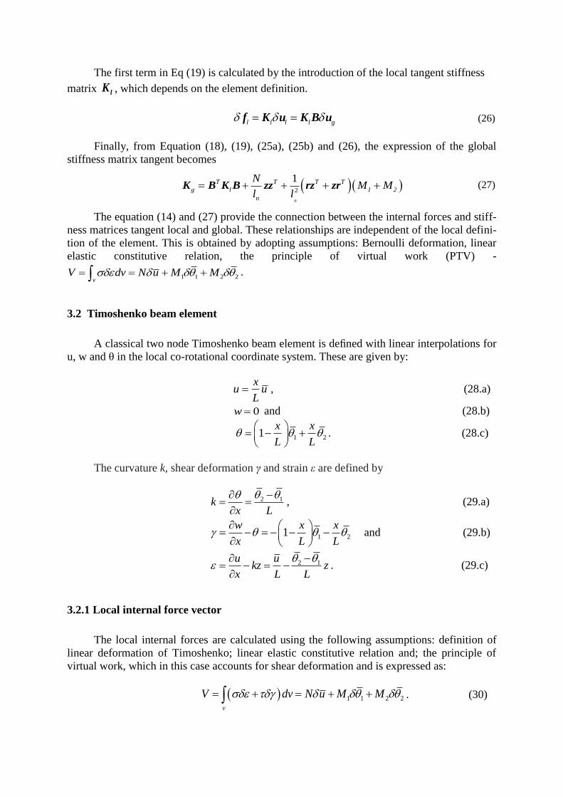
3.2 Timoshenko beam element

A classical two node Timoshenko beam element is defined with linear interpolations for

u, w and θ in the local co-rotational coordinate system. These are given by:

x

u uL

, (28.a)

0w and (28.b)

1 21x x

L L

. (28.c)

The curvature k, shear deformation γ and strain ε are defined by

2 1kx L

, (29.a)

1 21w x x

x L L

and (29.b)

2 1u ukz z

x L L

. (29.c)

3.2.1 Local internal force vector

The local internal forces are calculated using the following assumptions: definition of

linear deformation of Timoshenko; linear elastic constitutive relation and; the principle of

virtual work, which in this case accounts for shear deformation and is expressed as:

1 1 2 2

v

V dv N u M M . (30)

The calculation of and by differentiation of (29b-c) and its introduction in the

previous equation yields,

2 1 1 21v

x xV u z dv

L L L

. (31)

The internal forces are calculated of (30) and (31) with 2x L for avoid shear locking,

obtaining in this way:

v A

N dv dAL

, (32.a)

12 2

v A A

LM z dv zdA dA

L

and (32.b)

22 2

v A A

LM z dv zdA dA

L

. (32.c)

It is a new integration along the depth of the cross section of the element determining

the coefficients of internal forces in the same format that was implemented - Figure 3.

Figure 3. Algorithm to obtain the internal force vector location.

3.2.2 Local tangent stiffness matrix

The same assumptions used in the acquisition of the internal force vector are taken. The

consistent tangent operator defined by

do

elastic case : ;

elastoplastic case: call backward-Euler algorithm

end do

1 3

3 2

t t

t t

C C

C C

(33)

will be seen in Section 3.3. Equation (33) can be rewritten as

1 3t tC C (34.a)

1 2t tC C (34.b)

which, by using (29b–c) gives

1 31 2 1 2

2

t tC Cu z z

L (35.a)

3 21 2 1 2

2

t tC Cu z z

L (35.b)

Differentiation of (32) gives

A

N dA (36.a)

12A A

LM zdA dA (36.b)

22A A

LM zdA dA (36.c)

Finally, from (35) and (36), the local tangent stiffness matrix is

11 1

1t

A

NK C dA

u L

(37.a)

2122 1 3 2

1

1

4t t t

A A A

M LK C z dA C zdA C dA

L

(37.b)

2233 1 3 2

2

1

4t t t

A A A

M LK C z dA C zdA C dA

L

(37.c)

12 1 3

1

1 1

2t t

A A

NK C zdA C dA

L

(37.d)

13 1 3

2

1 1

2t t

A A

NK C zdA C dA

L

(37.e)

21 12K K , 31 13K K and 32 23K K .

Integrating numerically the previous coefficients along the depth of the cross section of

the element can be get them in the same format that was implemented (Figure 4).

Figure 4: Algorithm to obtain the tangent stiffness matrix.

3.3 Constitutive equations

In the plastic rate equations for the Timoshenko beam two strains , and two stress-

es , are involved. There are many different algorithms to integrate these equations and

among the iterative procedures, the most popular one is the backward-Euler scheme. It takes a

simple form in case of the von Mises yield criterion and it allows the generation of a con-

sistent tangent operator which maintains the quadratic convergence of the Newton-Raphson

method. The formulation descript here is mainly taken from Battini [2].

3.3.1 Plane beam equations

The relations for the plane beam are derived from the von Mises material with isotropic

hardening under plane stress conditions [3] by setting

do

elastic case :

elastoplastic case:

end do

0z (38)

The von Mises yield function is

1 22 2

0 03x xz ps e psf (39)

with

ps psdt 2 2 22

43

ps px pz px px pxz (40)

The hardening parameter H is calculated from the uniaxial stress-strain law

0

1

t

ps t

EH

E E

(41)

which gives

0 Y psH (42)

where Y is the yield stress. The Prandtl-Reuss flow rules associated to (39) are

2

26

px x

p pz x

e

pxz xz

f

aσ

(43)

The stress changes are related to the strain changes via

0 p σ C ε ε C ε a (44)

where

2

1 0

1 01

0 0 1 2

E

C

x

z

xz

σ

x

z

xz

ε (45)

By assuming that the stresses must remain on the yield surface in case of plastic loading

( 0 ), it is obtained

0

0

0T

T

ps

ps

f ff H

σ a σσ

(46)

which by using (44) gives

T

T H

a Cε

a Ca (47)

Since 0Z , the second equation of (44) gives

1

2

xz x

e

(48)

which by introduction in the first and third equations of (44) gives

xx x

e

E

3 xzxz xz

e

G

(49)

Substitution of equations (48) and (49) in (47) gives after some algebra

2 2 2

3

9

e x x xz xz

x xz e

E G

E G H

(50)

Finally, introducing (47) in (44) gives

T

t T H

aa Cσ C ε C I ε

aCa (51)

where tC is the tangent operator. The backward-Euler algorithm shown in Figure 6 consists in

applying an elastic forward step ( AB ) followed by a return mapping ( BC ) on the yield sur-

face – Figure 5.

C B C A C σ σ Ca σ C Ca (52)

Figure 5: Bacward-Euler scheme.

The vector Ca is normal to the yield surface at C, which is not known and therefore an

iterative procedure must be used. Since 0zC zA , the second equation of (52) gives

2 12

xCz x

eC

(53)

which, by substitution into the first and third equations, gives after some algebra

xCxC xA z

eC

E

(54.a)

3 xzCxzC xzA xz

eC

GE

(54.b)

By introducing the notations

x xz xz (55)

and new definitions for C ,σ , ε , a

0

0

E

G

C

σ

ε (56)

equations (43), (49), (50) and (54) can be combined and rewritten as

3

p

e

ε a (57)

p σ C ε ε C ε a (58)

T

T H

a Cε

a Ca (59)

C B C A C σ σ Ca σ C Ca (60)

It is therefore proved by comparing (44), (47) and (52) with (58), (59) and (60) that the

equations for the plane beam can be written in the same form as those under plane stress

conditions. It can be noted that the elastic forward step in the backward-Euler scheme does

not give 0zB , but the Equation (60) proves that zB does not need to be calculated.

3.3.2 Backward-Euler scheme

The algorithm of the backward-Euler scheme is taken from Battini [2]. The first estima-

tion of Cσ is calculated with

C B B A B σ σ Ca σ C Ca (61)

where Ba is calculated from (57) and is determined from a first order Taylor expansion of

the yield function around point B

0

0

TT

B B ps B B B

ps

f ff f f H

σ a σ

σ (62)

Bσ is the calculated from (58) as

B B σ C a (63)

with ε 0 since the total strain has already been applied in the elastic step (AB). Introducing

(62) in (63) and setting 0f gives

B

T

B B

f

H

a Ca (64)

Equation (61) gives stresses which do not satisfy the yield function since the normal at

B is not the same as the normal at the final position C. The iterative process is performed by

introducing the vector r defined by the difference between the current stresses and the back-

ward-Euler ones

C B C r σ σ Ca (65)

A truncated Taylor expansion of (65) gives

0

ar r σ Ca C σ

σ (66)

where

22

2 3 2

3

e

f

a

σ σ (67)

and σ is the change in Cσ and is the change in Δλ. The subscript C is from now dropped in

order to simplify the notations (all the notations without subscripts refer to C). Setting r to

zero in (66) gives

1

1

0 0

aσ I C r Ca Q r Ca

σ (68)

A truncated Taylor expansion of the yield function at C gives

00 0

0

TT

ps B

ps

f ff f f H

σ a σ

σ (69)

further, setting 0f and using (68) gives

1

0 0

1

T

T

f r

H

a Q

a Q a (70)

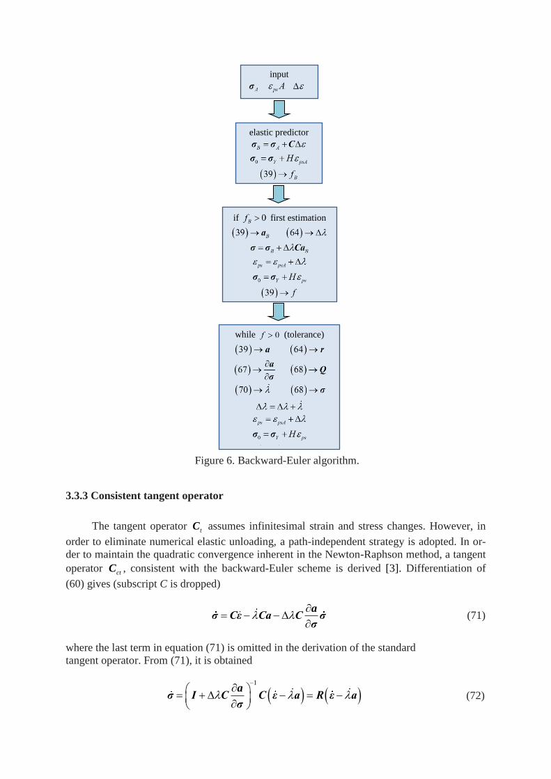
Figure 6. Backward-Euler algorithm.

3.3.3 Consistent tangent operator

The tangent operator tC assumes infinitesimal strain and stress changes. However, in

order to eliminate numerical elastic unloading, a path-independent strategy is adopted. In or-

der to maintain the quadratic convergence inherent in the Newton-Raphson method, a tangent

operator ctC , consistent with the backward-Euler scheme is derived [3]. Differentiation of

(60) gives (subscript C is dropped)

aσ Cε Ca C σ

σ (71)

where the last term in equation (71) is omitted in the derivation of the standard

tangent operator. From (71), it is obtained

1

aσ I C C ε a R ε a

σ (72)

input

elastic predictor

if first estimation

while (tolerance)

The stresses must remain on the yield surface, which, from (46), gives

0T Tf a H a H σ R ε a (73)

and hence

T

T H

a Rε

a Ra (74)

Introducing (74) in (72) finally gives

T

ct T H

aa Rσ C ε R I ε

a Ra (75)

4. NUMERICAL EXAMPLES

4.1 Lee’s frame

The loading conditions, boundary, geometry and material parameters of structure are

shown in Figure 4. This frame was shown by Lee [9] for analysis of large displacement and

stability of elastic frames. Battini [2], in turn, used to study beam elements co-rotational in-

stability problems. The equilibrium trajectories of the structure for linear analysis are known

in the literature as snap-back in the degree of freedom (DOF) u and snap-through in the DOF

v, so there are two points limit in the load-displacement diagram – Figure 7.

Figure 7. Geometry, boundary conditions and physical parameters.

E = 720

= 0,3

Et = E/10

y = 10,44

It is shown in the Figure 8 that the results are practically the same when using points 7

or 15 Gauss along the depth of the beam. The elastoplastic response (Figure 9 above) in turn

both the DOF u and v have the snap-through behavior. As we can see, there is an excellent

convergence of the results obtained in this study with those obtained by Battini [2].

Figure 8. Elastic response - mesh with 20 elements – 7 and 15 Gauss points.

Figure 9. Elastoplastic response - mesh with 20 elements – 7 Gauss points.

4.2 Williams toggle frame

In this work it was used an equivalent rectangular section (with the same inertia and ar-

ea) to simulate a circular section. The loading conditions, geometric (real and equivalent),

boundary, and the material properties of toggle frame studied here can be seen in Figure 10. It

was originally solved analytical and experimentally by Williams [12]. Remo [4] also studied

in the investigation of large displacements experienced by inelastic frames.

As can be seen by snap-through elastic and elastoplastic paths (Figure 10), although

they have the same behavior, the responses of this analysis are less stiffness than those ob-

tained by Remo [4].

Figure 10: Dimensions, boundary conditions and material properties.

Figure 11: Response elastic and elastoplastic - mesh with 20 elements and 15 Gauss points.

E = 107 = 0,3

Et = E/2 y = 3x103

This fact is probably due to the mixed formulation implemented by this author whereas

this article uses a formulation in displacement. Furthermore, in the present work we adopted

the hypothesis of an equivalent rectangular section.

5. CONCLUSIONS

This study evaluated the efficiency of a beam element 2D Timoshenko applied in a finite

element program that takes into account the geometric and physics nonlinearity. In the exam-

ples studied – Lee´s frames and Williams toggle frames - there is a decrease in bearing ca-

pacity of the structure when one considers the phenomenon of elastoplasticity. In addition,

highlights the ability of corotational formulation to capture large displacements and rotations.

In elastoplastic analysis, the use of fifteen points Gauss at the time of cross-section instead

of seven does not produce a significant improvement in results. Finally, we conclude that the

use of simple strategy of equivalent rectangular sections in the study of other types of cross

sections provide satisfactory results.

Acknowledgements

The authors wish to express gratitude for the financial support received from the CNPq for

financial support and the Postgraduate Program in Structures and Civil Construction -

PECC/UnB.

6. REFERENCES

[1] Argyris, J.H., “Continua and discontinua”, Proceedings 1st Conference on Matrix Meth-

ods in Structural Mechanics, AFFDL-TR-66-80, Air Force Institute of Tecnology, Dayton,

Ohio-USA, 1965.

[2] Battini, J.M., “Co-rotational beam elements in instability problems”, Ph.D Thesis, Royal

Institute of Tecnology - Departament of Mechanics, Stockholm / Sweeden, 2002.

[3] Crisfield, M.A., “Non-linear finite element analysis of solids and structures”, Volume 1:

Essential, John Wiley & Sons, Chichester, UK, 1991.

[4] De Souza, R. M., "Force-Based Finite Element for Large Displacement Inelastic Analsysis

of Frames", Ph.D. Dissertation, University of California at Berkeley, Berkeley, CA, USA,

2000.

[5] Felippa, C.A., “Non-linear finite element methods / NFEM”, Lecture notes for the course

non-linear finite element methods, Center for Aerospace Structures, University of Colora-

do, Boulder/USA, 2001.

[6] J. N. Reddy., “An Introduction to Nonlinear Finite Element Analysis”, Oxford University

Press : Oxford, U.K, 2004.

[7] Owen, D.R.J., Hinton, E., Finite Elements in Plasticity: Theory and Practice, Pineridge.

Swansea, U.K, 1980.

[8] Lemaitre, J., Chaboche, J-L., Mechanics of Solids Materials, Cambrige University Press,

Cambrige, , U.K, 1994.

[9] Lee, S. L., Manuel F. S., & Rossow, E. C., Large deflection analysis and stability of elas-

tic frames. J. Eng. Mech. Div. ASCE 94 EM2, pp. 521-547, 1968.

[10] Menin, R. C. G., “Application of co-rotational description in geometric nonlinear analy-

sis of structures discretized by finite elements of trusses, beams and shells”, PhD thesis,

E.TD-004A/06, Brasília : ENC/FT/UnB, 2006.

[11] Simo, J. C., Computational Inelastic, Interdisciplinary Apllied Mathematics, vol. 7,

Springer, New York, USA, 1998.

[12] Williams, F. W., ‘An approach to the nonlinear behaviour of the members of a rigid

jointed plane framework with finite deflection’, Quart. J. Mech. Appl. Maths. 17(4), 451–

469, 1964.