I SLAC - PUB - 3545 January 1985 (4

NONLINEAR BEAM-BEAM RESONANCES*

A. W. CHAO SSC Central Design Group

University Research Association c(o Lawrence Berkeley Labo_ratoIy _

Uniuersity of California, Berkeley, California 94 7.20

P. BAMBADE AND W. T. WENG Stanford Linear Accelerator Center

Stanford University, Stanford, California 94305

In a colliding beam storage ring, a major source of nonlinear resonance excitation resides in the beam-beam collisions as the stored beams repeatedly cross each other. During such collisions, particles in each beam see the electromagnetic field generated by the counter rotating beam. The beam-beam collisions therefore perturb the particle motion, causing

-1. the transverse beam size to blow up and loss of luminosity

2. the beam lifetime to be reduced

3. and rapid beam loss as beam intensity increases beyond a more or less distinct threshold.

Considerable efforts, both experimental and theoretical, have brought some insight into the beam- beam instability problem and often led to improvements in luminosity. But the nature of the instability and its associated underlying mechanism(s) are not yet fully understood and remain an outstanding problem for the designers of colliding beam storage rings.

The beam-beam problem will be reviewed by other authors of this school (Seeman on ex- periments, Schonfeld on models and Myers on simulations). Nonlinear resonance behavior is the underlying process in these reviews and it is the job of this lecture to identify the role of nonlin- ear resonances in the beam-beam problem. To reduce the scope of this lecture, we will consider only head-on collisions of bunched beams. For the sign convention of the beam-beam force, we assume the two colliding beams to have opposite charges. We also assume that the reader is at least somewhat familiar with Hamiltonian dynamics and some basic facts about the beam-beam interaction. For part of the discussions on coherent beam-beam effects, we assume the reader has some knowledge about the Vlasov equation.

t Wcrrk supported in part by the Department of Energy, contracts DE-AC03-76SF00515 and DE-AC02-76CH03001.

Invited paper present at the Joint US/CERN School on Particle Accelerators, Sardinia, Italy, January 31 - February 5, 1985.

1. Some Experimental Observations

We first describe a few experimental observations with no intention of being complete. Al- though details of these experimental results may not always easy to interpret or even to reproduce, the fact that nonlinear resonances play a dominating role in the beam-beam phenomena should be clearly demonstrated by these examples.

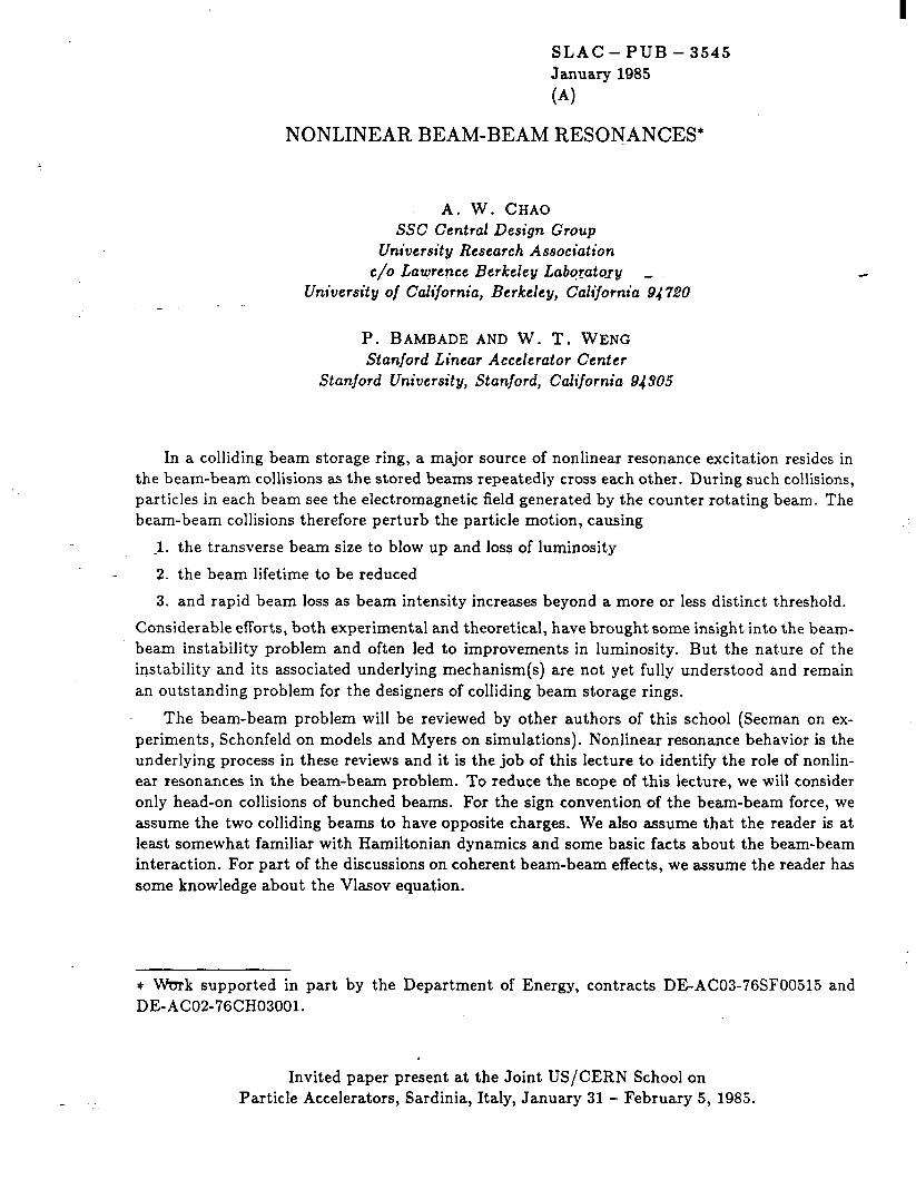
One of the simplest experiments one can think of consists of colliding a strong beam with a weak one and then observing the vertical sizes of the two beams as the vertical tune is varied. Results from such an experiment with ACO’ are shown in Fig. 1. In such a strong-weak situation, only the weak beam is affected by the beam-beam interaction. Figure 1 clearly shows that the weak beam blows up every time the vertical tune approaches a fractional value. Note that the strong beam also blows up near. the resonances I+ = pV and VJ = 263. These blow-ups are not- caused by the beam-beam interaction but by the residual field errors in the storage ring. _

In the case of two strong beams, the situation is more complex. Unlike the strong-weak case, now both beams are perturbed. This means that not only can single particles be excited incoher- ently but the colliding bunches can also be driven coherently, thus acting as a system of coupled oscillators. Both the incoherent and the coherent aspects have been used to explain observed results but it is not always easy to distinguish them. Theoretically both effects exhibit nonlinear resonance behavior and are expected to play important roles in the beam-beam phenomenon.

Fig. 1. AC0 beam profiles as ver- tical time is varied.

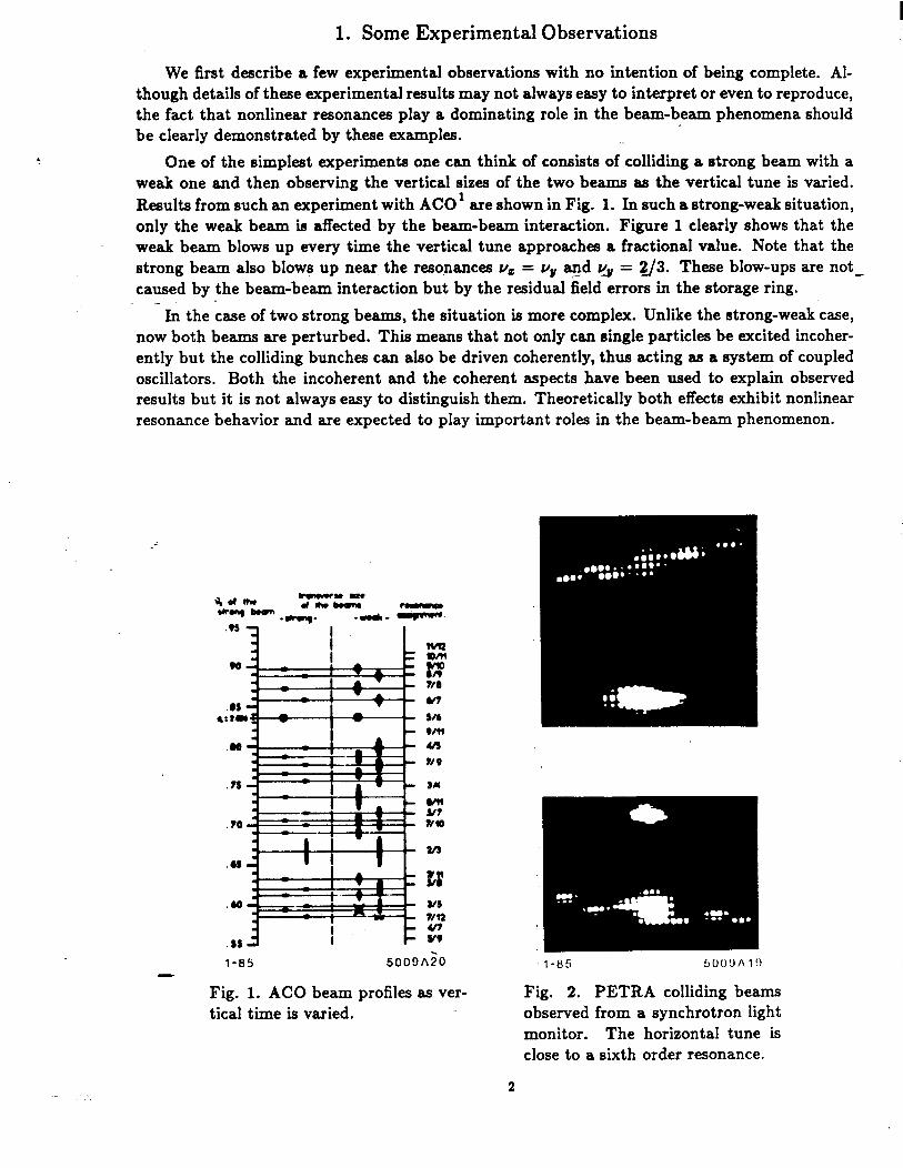
Fig. 2. PETRA colliding beams observed from a synchrotron light monitor. The horizontal tune is close to a sixth order resonance.

2

In early days of PETRA, colliding beams exhibited distributions shown in Fig. 2 in the neigh- borhood of a sixth order horizontal resonance.2 The beam distributions were distorted strongly into a set of islands, a behavior that is unmistakenly that caused by a nonlinear resonance.

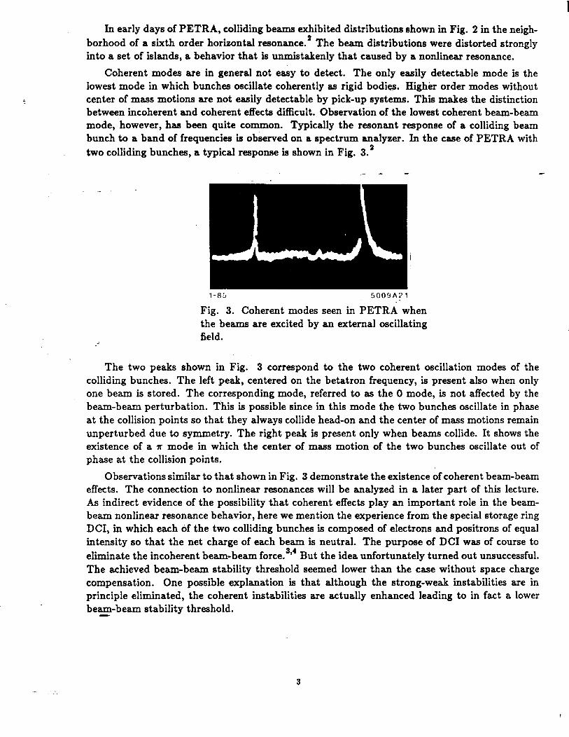
Coherent modes are in general not easy to detect. The only easily detectable mode is the lowest mode in which bunches oscillate coherently as rigid bodies. Higher order modes without center of mass motions are not easily detectable by pick-up systems. This makes the distinction between incoherent and coherent effects difficult. Observation of the lowest coherent beam-beam mode, however, has been quite common. Typically the resonant response of a colliding beam bunch to a band of frequencies is observed on a spectrum analyzer. In the case of PETRA with two colliding bunches, a typical response is shown in Fig. 3.2

l-83 500YA2 1

Fig. 3. Coherent modes seen in PETRA when the beams are excited by an external oscillating field.

The two peaks shown in Fig. 3 correspond to the two coherent oscillation modes of the colliding bunches. The left peak, centered on the betatron frequency, is present also when only one beam is stored. The corresponding mode, referred to as the 0 mode, is not affected by the beam-beam perturbation. This is possible since in this mode the two bunches oscillate in phase at the collision points so that they always collide head-on and the center of mass motions remain unperturbed due to symmetry. The right peak is present only when beams collide. It shows the existence of a a mode in which the center of mass motion of the two bunches oscillate out of phase at the collision points.

Observations similar to that shown in Fig. 3 demonstrate the existence of coherent beam-beam effects. The connection to nonlinear resonances will be analyzed in a later part of this lecture. As indirect evidence of the possibility that coherent effects play an important role in the beam- beam nonlinear resonance behavior, here we mention the experience from the special storage ring DCI, in which each of the two colliding bunches is composed of electrons and positrons of equal intensity so that the net charge of each beam is neutral. The purpose of DC1 was of course to eliminate the incoherent beam-beam force. 3’4 But the idea unfortunately turned out unsuccessful. The achieved beam-beam stability threshold seemed lower than the case without space charge compensation. One possible explanation is that although the strong-weak instabilities are in principle eliminated, the coherent instabilities are actually enhanced leading to in fact a lower beam-beam stability threshold. -

2. The Strong-Weak Single Resonance Model

In this section we will develop the single resonance analysis that is applicable to the strong- weak case of the beam-beam interaction. In this case, the strong beam is unperturbed by the beam-beam interaction; motions of the weak beam particles are then analysed in the presence of the nonlinear electromagnetic force produced by the strong beam at the collision points.

2.1 THE FORMALISM

In the strong-weak picture, the motion of a test particle in the weak beam is governed by the Hamiltonian5”

H=Ho+Hl < - s

= 5 (PZ + Kzz2) + f (Pi + KyY”) + qw/) 6p(s) (2.1)

where U(z, y) is the equivalent potential produced by the strong beam, z and y are the horizontal and vertical coordinates that describe the test particle motion. The C-function represents the periodic collisions with a period 2sR/S where R is the average radius of the storage ring and S is the number of collision points around the ring. The unperturbed Hamiltonian Ho represents the usual two dimensional betatron motions with focussing structures described by K,(s) and K,(s).

The equations of motion described by the Hamiltonian (2.1) are

$ + Kz(s)z = +(s) , 2 = z,y (2.2) The potential U depends on the distribution of the strong beam at the collision points. Assuming

- the strong beam has an upright bi-gaussian distribution, the potential can be written a~‘*~

U(z, y) = $ (2-3)

where rc = e2/mc2 is the classical radius of the particle, 7 is the relativistic factor, N is the number of particles per bunch and crz,y are the rms beam dimensions of the strong beam at the collision points. Throughout this section on strong-weak single resonance treatment, we will assume the gaussian potential given by Eq. (2.3).

‘Equations (2.1) and (2.2) can be solved in various stages of approximations and sophistica- tions. The simplest treatment is to consider only the linear effects by Taylor expanding U(z, y) and keeping only terms quadratic in z and y. The problem is then solved exactly in the same way as ordinary gradient perturbations. The linear beam-beam perturbations give rise to betatron tune shifts & which are given by

where /?& are the betatron functions at the collision point. %I the linear approximation, the z- and the y-motions are decoupled. The motion in each

dimension is completely determined by tw-o parameters, i.e. the betatron tune per revolution Y and the beam-beam strength parameter [. The simplest resonance effect manifest itself when v is sufficiently close to a half integer, the particle motion becomes unstable due to the gradient perturbation of the beam-beam force.

4

When the complete potential U is taken into account, the particle motion is affected by the beam-beam perturbation whenever a nonlinear resonance condition is approximately satisfied

where n, m and k are integers. The even coefficients in front of-u, and VV is due to the polarity of the beam-beam force. Resonances with odd coefficients are not excited except for non-head-on collisions, which we do not consider in this lecture. Extension of single resonance analysis to include the non-head-on cases is straightforward with proper modifications on the beam-beam force.

To treat the general strong-weak problem, it is a matter of taste whether to start with the Hamiltonian (2.1) or with the equations of motion (22),-eachgives the same answer. The Hamiltoni-an approach will be adopted here. In the following we will assume that & = cv = 6.

The first step is to make a canonical transformation on the Hamiltonian H to remove the time-dependence from Ho, thus defining an equivalent harmonic oscillator with frequencies u, and uv. The transformation has the generating function

2 W5Y,4zdy) = -; c -

*=2,Y i%(s) tanpz [ (4 P:

2 1 with

where p,(s) and &( ) s are the betatron functions defined by Courant and Snyder.g _ The relation between the old coordinates (z, pz) and new coordinates (J,, &) is

Pz = - P: sin& - -zcos& , z=x,y

We then normalize the action variables by

JZ a* = - cz + cy ’

2 = x,y

(2.7)

(24

where cz,y = &,/&, are the natural emittances of the strong beam. We also will change the time variable s to the azimuthal angle B = s/R.

Assuming equal linear tune shifts in the x and y planes, the new Hamiltonian becomes

-

where a = uY/uZ is the aspect ratio of the strong beam distribution. Note that the periodic delta-function in s has been replaced by infinite series of sinusoidal terms in 8.

5

So far the manipulation on the Hamiltonian has been only mathematical. The physics comes in the next step - the “smooth approximation”. To do that, we assume there is one and only one dominating nonlinear resonance that determines the motion of the weak beam particles.

Let the resonance be that of Eq. (2.5). Note that the Hamiltonian (2.9) contains complicated dependences on 8, &, and 4,,. In the smooth approximation, we need to remove the “fast oscil- lating” terms and extract only the “slowly varying” terms in the Hamiltonian. To do so, a triple Fourier expansion in 8, 4% and d,, is performed on (2.9). Keeping only the slowly varying terms, we obtain a new Hamiltonian

H(dz, du, a, q,, 0) = uzaz + JQ,~, + SC [Hoo(az, q,) (2.10)

+ 26-l) n+m&m(az, a,,) ys(ke + 2,n& + 2y+,)]

-There are two-beam-beam terms in (2.10). The first term is independent of 8, 4% and &. The second term contains the Fourier component in the slow variable kS8+2nq5,+2m& 7% functions Hoo (oz, ov) and Hnm (a,, cy,,) are the Fourier components of the beam-beam perturbation

00

/

P H nm = dt nm (2.11)

0

where Pnm = 1 if n = m = 0 and 0 otherwise, In and Im are Bessel functions. There are two invariants for the smoothed Hamiltonian (2.10). The first one is

C= -ma= + nay (2.12)

For a one-dimensional resonance (n = 0 or m = 0), it trivially means that the other dimension is not affected, and is thus redundant in the treatment. For a twc+dimensional resonance, it expresses the exchange of energy between the two coupled dimensions under the constraint of (2.12) and renders the problem effectively one-dimensional.

We now perform another canonical transformation using the generating function

~2Wz,~y,K,mq = --$& [K(2n& + 2m4, + ke) + C(%u$, - 2m4,)]

The dynamical variables for the effective coupled dimension are

(2.13)

K= - (maz + nay)

where rl, is the slow phase. The corresponding Hamiltonian is’

H(Kt$) = -2 +SC [Hoo(K) + 2(-l)m+nHnm(K)cos(4mnt,b)] (2.15)

(2.14)

- where 6u = 2nu, + 2mu,, + k specifies the distance from the exact location of the resonance. Note that this Hamiltonian is independent of the time variable 8, meaning it is the second constant of the motion. The functions Ho0 and H nm are the characteristic functions of the beam-beam problem in the single resonance picture.

6

2.2 PHASE SPACE STRUCTURE

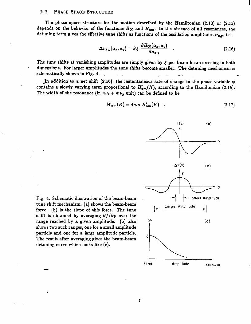
The phase space structure for the motion described by the Hamiltonian (2.10) or (2.15) depends on the behavior of the functions I& and II,,,,,. In the absence of all resonances, the detuning term gives the effective tune shifts as functions of the oscillation amplitudes CY=,~, i.e.

(2.16)

The tune shifts at vanishing amplitudes are simply given by [ per beam-beam crossing in both dimensions. For larger amplitudes the tune shifts become smaller. The detuning mechanism is schematically shown in Fig. 4. F - e

-In addition to a net shift (2.16), the instantaneous rate of change in the phase variable ?,6 contains a slowly varying term proportional to H;,(K), according to the Hamiltonian (2.15). The width of the resonance (in nv, + mug unit) can be defined to be

Wnm(K) = 4mn H:,(K) . (2.17)

Ady) (bl

ly --it Small Amplitude Fig. 4. Schematic illustration of the beam-beam

tune shift mechanism. (a) shows the beam-beam force. (b) is the slope of this force. The tune shift is obtained by averaging aj/ZIy over the range reached by a given amplitude. (b) also shows two such ranges, one for a small amplitude particle and one for a large amplitude particle. The result after averaging gives the beam-beam detuning curve which looks like (c).

t Large Amplitu’de

AU

‘\

(cl

t

1 t-85 Amplitude 5009AlS

-

It should be pointed out that (2.17) is the simplest possible definition of resonance width. More sophisticated definitions taking more carefully into account the phase space structure also exist, but will not be considered in the following analysis.

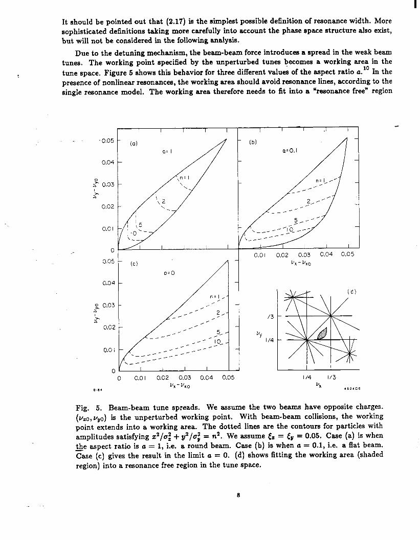
Due to the detuning mechanism, the beam-beam force introduces a spread in the weak beam tunes. The working point specified by the unperturbed tunes becomes a working area in the tune space. Figure 5 shows this behavior for three different values of the aspect ratio a.” In the presence of nonlinear resonances, the working area should avoid resonance lines, according to the single resonance model. The working area therefore needs to fit into a “resonance free” region

-0.05

0.04

0 0 0.0 I 0.02 0.03 0.04 0.05

ux-uxo 8-84

I I I I I

(a)

I I I I I

I /4 l/3 VX .624C5

Fig. 5. Beam-beam tune spreads. We assume the two beams have opposite charges. (v,o,v~o) is the unperturbed working point. With beam-beam collisions, the working point extends into a working area. The dotted lines are the contours for particles with amplitudes satisfying x2/u: + g”/c$ = n2. We assume & = &, = 0.05. Case (a) is when the aspect ratio is a = 1, i.e. a round beam. Case (b) is when a = 0.1, i.e. a flat beam. Case (c) gives the result in the limit a; = 0. (d) shows fitting the working area (shaded region) into a resonance free region in the tune space.

I in the tune space, as shown in Fig. 5(d). For a flat beam with small aspect ratio, an inspection of the shape of the working area in Fig. 5 shows that it is better to chooee the unperturbed working point to lie on the lower right side of the destructive resonances than to the upper left side. In particular, when applied to the diagonal 2u, - 2v,, = n resonance, this means the unperturbed working point should be below the resonance line.”

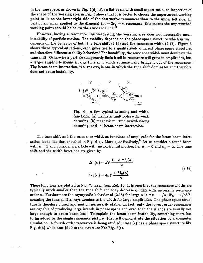
However, having a resonance line trespassing the working area does not necessarily mean instability of particle motion. The stability depends on the phase space structure which in turn depends on the behavior of both the tune shift (2.16) and the resonance width (2.17). Figure 6 shows three typical situations, each gives rise to a qualitatively different phase space structure, and therefore different stability behavior.6 For instability, the resonance width must dominate the tune shift. Otherwise a particle temporarily finds itself in resonance will grow in amplitudes, but a larger amplitude means a large tune- shift which automatically brings it out of the resonance. -

-The beam-beam interaction, it turns out, is one in which the tune shift dominates and therefore does not cause instability.

k

Fig. 6. A few typical detuning and width functions: (a) magnetic multipoles with weak

-- detuning; (b) magnetic multipoles with strong detuning; and (c) beam-beam interaction.

The tune shift and the resonance width as functions of amplitude for the beam-beam inter- action looks like that sketched in Fig. 6(c). More quantitatively,’ let us consider a round beam with a = 1 and consider a particle with no horizontal motion, i.e. cxz = 0 and cyv = cy. The tune shift and the width functions are given by

A+) = SC 1 - e-V&)

a (2.18)

, W&y) = 4&?( e-41n(a) a

These functions are plotted in Fig. 7, taken from Ref. 14. It is seen that the resonance widths are typically much smaller than the tune shift and they decrease quickly with increasing resonance order n. Furthermore the asymptotic behavior of (2.18) for large (Y is Au -+ l/a, W, + l/asi2, meaning the tune shift always dominates the width for large amplitudes. The phase space struc- ture is therefore closed and motion necessarily stable. In fact, only the lowest order resonances are capable of producing large islands in phase space and even then the islands are usually not large enough to cause beam loss. To explain the beam-beam instability, something more has to L added to the single resonance picture. Figure 8 demonstrate the situation by a computer simulation. A fourth order resonance is being studied. Case (c) has a phase space structure like Fig. 6(b) while case (d) has the structure like Fig. 6(c).

9

Fig. 7. Beam-beam detuning (a) and width (b) in the case of a round beam.

-- 0 I 2 3 4 5

l-85 X/CT 500’JA:i

2.3 VERTICAL BLOW-UP OF FLAT BEAMS

In the following few sections, a few variations on the single resonance models will be briefly discussed. As mentioned before, a strict single resonance model does not explain the observed beam-beam instability. Before we describe the variations, however, we will discuss in this section how a nonlinear single resonance can cause sizable blow-up in the tails of the vertical distribution of a flat beam.

The point is quite simple. In case of coupled nonlinear resonances, there is exchange of horizontal and vertical energies. The exchange obeys the two constants of the motion (2.12) and (2.15). For a flat beam, the horizontal energy is much larger than the vertical one and a small energy exchange can cause a sizable increase in the vertical distribution although the effect on the horizontal distribution can be quite small. This blow-up in the vertical beam size does not cause direct beam loss, but if the blow-up is large enough, it can cause loss in beam lifetime.

As an illustration, we study the effect of the lowest order difference resonance6’1’

2u, - 23 - k w 0 (2.19)

corresponding to n = 1, m = -1 in (2.5). The two invariants are -

c = a, + ay

H ma = y + Se [Ho@) - 2H&f) cos(4$)] (2.20)

10

4 I-‘“““” 1 ” ” ” ” ” ~““““““I”“““~ . /

2

v 0

-2

(O’ ,.....t.. . . ,:’ : ; ..: : .;. .’ ,’ ,.:: . . .‘.‘. “‘, ,.

: : ,.:. ,: . . . . ::I:: ..;,;;& ..,,,:

..” ..%....., .;, ; :’ ..’ : : : :’ ; ,. i : :. i i

~~~~~~,.~,~ lb) 1

‘... ,, ,;’ ,:,: : .;. .“(. .._,,,,,(.. ..“. ,: :

1

. . ‘.... ,c;,.:;: ..:..

.,.;.

,_....

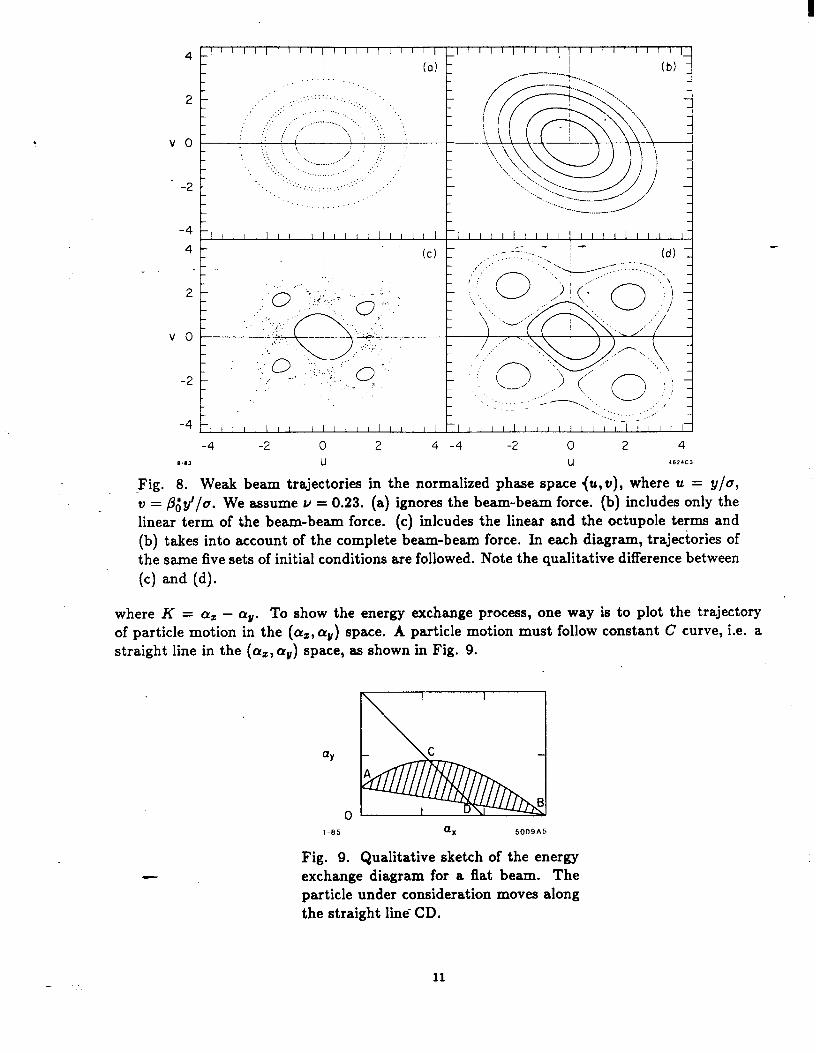
-Fig. 8. Weak beam trajectories in the normalized phase space (u, u), where u = y/a, u = PO* y’/o. We assume u = 0.23. (a) ignores the beam-beam force. (b) includes only the linear term of the beam-beam force. (c) inlcudes the linear and the octupole terms and (b) takes into account of the complete beam-beam force. In each diagram, trajectories of the same five sets of initial conditions are followed. Note the qualitative difference between (c) and (d).

where K = cyz - cyI. To show the energy exchange process, one way is to plot the trajectory of particle motion in the (oZ, cu,,) space. A particle motion must follow constant C curve, i.e. a straight line in the (cyz, av) space, as shown in Fig. 9.

-

ax 5009A5

Fig. 9. Qualitative sketch of the energy exchange diagram for a flat beam. The particle under consideration moves along the straight line CD.

- 11

Consider a particle with initial amplitudes satisfying $ + 5 = n2. Its subsequent motion will trace out a trajectory along the constant C straight lines between two extreme end points. The boundary of the shaded area in Fig. 9 gives the end points for given n. The small aspect ratio is indicated by the fact the distance OA is much less than OB. The particle moves back and forth along the straight line CD. The energy exchange is such that a small change in the horizontal emittance gives rise to a large change in the vertical emittance. Figures lo(a)-(d) give the energy exchange diagrams for a beam with aspect ratio of l/16. Three values of Au/Se are used. The energy transfer is most pronounced for the case with 6r~/Sc = -0.25. This is consistent with the “preferred side” effect mentioned when discussing Fig. 5.

“Y QY 11.32 8

- 9.80 6

8.00 4

5.64 2

2.83 1.55 0

“Y QY Il.32 8

9.80 6

8.00 ‘4

5.64 2

2.83 1.55 0

0 2 4 6 8ax I-85 I.41 2.00 2.45 2.83 5O,i!#Ab nx

0 2 4 6 8ax 0 2 4 6 8ax

1.41 2.00 2.45 2.83 nx I.41 2.00 2.45 2.83 nx

“Y QY Il.32 8

9.80 6

8.00 4

5.64 2

“Y QY 4.89

4.00 I.

2.83

I.41

0.2 0.6 1.0 1.5 2.0 ax 0.7 1.0 1.22 2.41 nx

Fig. 10. Transformation of beam envelopes:6 (a) below the resonance (Aq/Se = 0.25); (b) right on the resonance (Aq/Se = 0.00); (c) above the resonance (Aq/S[ = -0.25); and (d) same as (c), at smaller amplitude.

2.4 OVERLAPPING RESONANCES

The first variation of the single resonance model we will discuss is to consider the effects of the other resonances. In making the single resonance approximation, we have assumed that the dense web of higher order resonances have negligible effect on particle motion. In fact we know that in such a non-integrable system, part of the trajectories will exhibit chaotic behavior, especially neaethe island separatrices. The integrable approximation used in the single resonance model holds only if such chaos remains constricted to very limited regions. As the beam-beam strength is increased and islands become larger, chaotic behavior will be enhanced.

Figure 11 qualitatively illustrates such a behavior. Figure 11(a) shows the detuning curve in which two resonant tune values are present in the tune spread range. Below the stochastic

._ 12

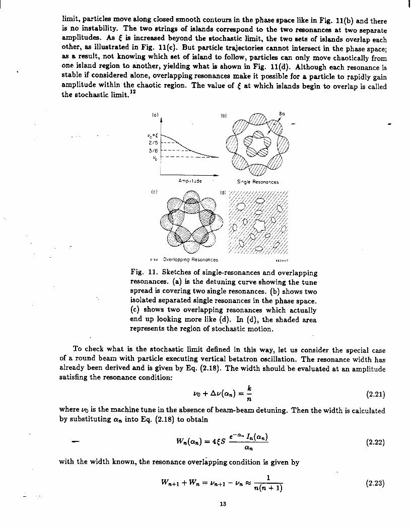
limit, particles move along closed smooth contours in the phase space like in Fig. 11(b) and there is no instability. The two strings of islands correspond to the two resonances at two separate amplitudes. As t is increased beyond the stochastic limit, the two sets of islands overlap each other, as illustrated in Fig. 11(c). But particle trajectories cannot intersect in the phase space; as a result, not knowing which set of island to follow, particles can only move chaotically from one island region to another, yielding what is shown in Fig. 11(d). Although each resonance is stable if considered alone, overlapping resonances make it possible for a particle to rapidly gain amplitude within the chaotic region. The value of e at which islands begin to overlap is called the stochastic limit. l2

Amplitude Single Resonances

8-8~ OverloppIng Resonances

Fig. 11. Sketches of single-resonances and overlapping resonances. (a) is the detuning curve showing the tune spread is covering two single resonances. (b) shows two isolated separated single resonances in the phase space. (c) shows two overlapping resonances which actually end up looking more like (d). In (d), the shaded area represents the region of stochastic motion.

To check what is the stochastic limit defined in this way, let us consider the special case of a round beam with particle executing vertical betatron oscillation. The resonance width has already been derived and is given by Eq. (2.18). The width should be evaluated at an amplitude satisfing the resonance condition:

uo + Av(cz,J = ; (2.21)

where vo is the machine tune in the absence of beam-beam detuning. Then the width is calculated by substituting a, into Eq. (2.18) to obtain

- Wn(an) = 4cs e-a”2(a.) (2.22)

with the width known, the resonance overlapping condition is given by

W 1

n+l + Wn = vn+l - Vn e n(n + 1) (2.23)

- 13

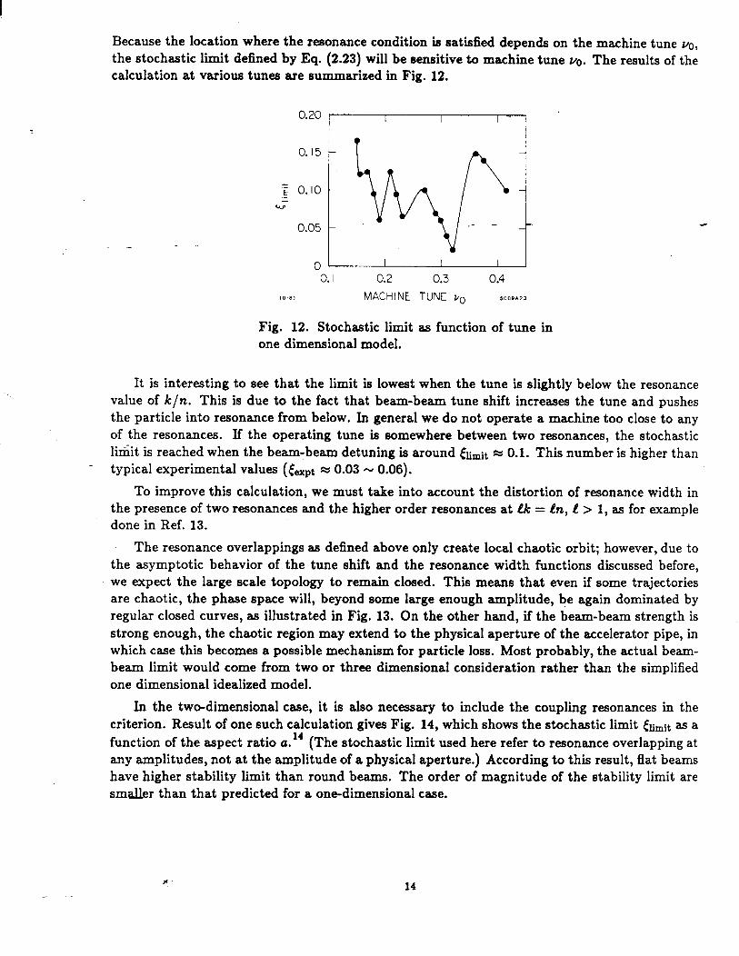
Because the location where the resonance condition is satisfied depends on the machine tune ~0, the stochastic limit defined by Eq. (2.23) will be sensitive to machine tune uo. The results of the calculation at various tunes are summarized in Fig. 12.

0.20

0. I5

‘E 0.10 .- G

0.05

0

r

Fig. 12. Stochastic limit as function of tune in one dimensional model.

. . It is interesting to see that the limit is lowest when the tune is slightly below the resonance

value of k/n. This is due to the fact that beam-beam tune shift increases the tune and pushes the particle into resonance from below. In general we do not operate a machine too close to any of the resonances. If the operating tune is somewhere between two resonances, the stochastic limit is reached when the beam-beam detuning is around [timit w 0.1. This number is higher than

- typical experimental values ( eexpt % 0.03 - 0.06).

To improve this calculation, we must take into account the distortion of resonance width in the presence of two resonances and the higher order resonances at tk = fh, e > 1, as for example done in Ref. 13.

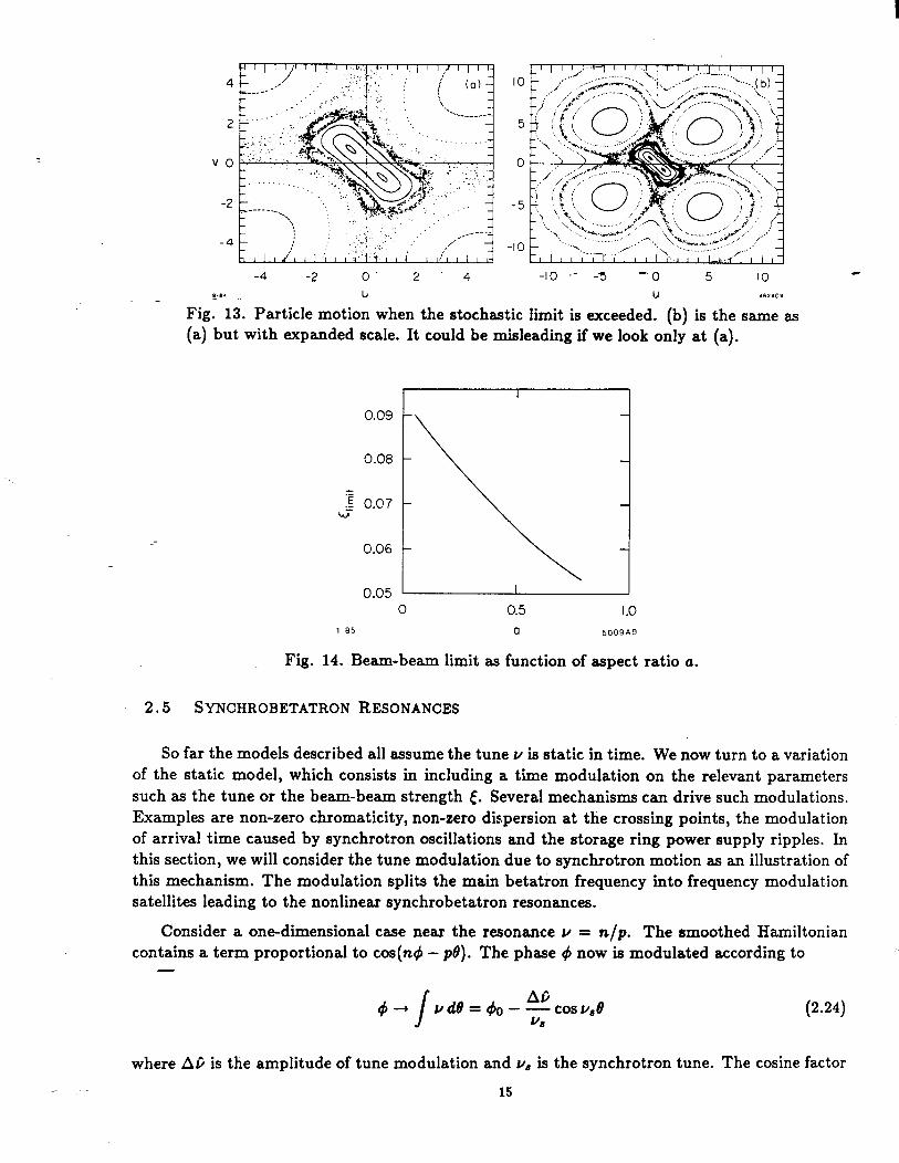
The resonance overlappings as defined above only create local chaotic orbit; however, due to the asymptotic behavior of the tune shift and the resonance width functions discussed before, we expect the large scale topology to remain closed. This means that even if some trajectories are chaotic, the phase space will, beyond some large enough amplitude, be again dominated by regular closed curves, as illustrated in Fig. 13. On the other hand, if the beam-beam strength is strong enough, the chaotic region may extend to the physical aperture of the accelerator pipe, in which case this becomes a possible mechanism for particle loss. Most probably, the actual beam- beam limit would come from two or three dimensional consideration rather than the simplified one dimensional idealized model.

In the two-dimensional case, it is also necessary to include the coupling resonances in the criterion. Result of one such calculation gives Fig. 14, which shows the stochastic limit &it as a function of the aspect ratio a.” (The stochastic limit used here refer to resonance overlapping at any amplitudes, not at the amplitude of a physical aperture.) According to this result, flat beams have higher stability limit than round beams. The order of magnitude of the stability limit are smaller than that predicted for a one-dimensional case.

14

-4 -2 0. 2 4 -IO’-3 “0 5 IO e_--

Fig. 13. Particle motioi when the stochastic limit is exceeded: (b) 4614CO

is the same as (a) but with expanded scale. It could be misleading if we look only at (a).

0.08

0.06

0.05 1 0 0.5 1.0

1-85 cl 5009AQ

Fig. 14. Beam-beam limit as function of aspect ratio a.

2.5 SYNCHROBETATRON RESONANCES

So far the models described all assume the tune u is static in time. We now turn to a variation of the static model, which consists in including a time modulation on the relevant parameters such as the tune or the beam-beam strength [. Several mechanisms can drive such modulations. Examples are non-zero chromaticity, non-zero dispersion at the crossing points, the modulation of arrival time caused by synchrotron oscillations and the storage ring power supply ripples. In this section, we will consider the tune modulation due to synchrotron motion as an illustration of this mechanism. The modulation splits the main betatron frequency into frequency modulation satellites leading to the nonlinear synchrobetatron resonances.

Consider a one-dimensional case near the resonance u = n/p. The smoothed Hamiltonian contains a term proportional to cos(ntj - ~8). The phase 4 now is modulated according to

-

t$-,/udt9=t$o-Clfcosu,,8 u.¶

(2.24)

where Afi is the amplitude of tune modulation and u, is the synchrotron tune. The cosine factor

15

in the Hamiltonian becomes

cos(n# - ~8) + co8 nf$o - ptJ - nAD - CO6 lJ,e

u, > (2.25)

cos(nt$o - pB i ku,t?) . The single betatron resonance therefore splits up into a spectrum of resonances spaced by us/n, i.e. the resonance conditions are

- P ku, u-z --- ) k= O,fl,iE2,:.. - n n

(2.26)-

The strength of these synchrobetatron resonances decreases with the resonance order according to Jk(nAP/u,).

It is clear that the existence of synchrobetatron resonances increases the density of resonances in the tune space, which reduces the stochastic limit. As a simple-minded illustration of this point, one can calculate the stochastic limit in the neighborhood of a single betatron resonance of a particular order n by asking if the widths of the synchrobetatron satellites corresponding to this resonance overlap. This calculation has been attempted for the Sp# using the parameters U8 = 4 x 10e3, Afi = 1.5 x 10B3 and n = 10. The resulted stochastic limit as a function of amplitude is tabulated below: l5

-- Amplitude (z/o) hi mit 2 1.1 x 10-2 3 3.8 x 1O-3 4 2.0 x 1o-3

We see that these [Emit values are much smaller than those discussed before without the synchrobetatron coupling and are more or less encouragingly in agreement with what has been observed in the SpfG. For electron storage rings, the value of u8 is much larger than that of the SP~LS’, this leads to larger spacing between adjacent synchrobetatron resonances and thus higher stochastic limit in this model.

There are other sources that introduces more resonances than the synchrotron motion. For example, we mentioned before that if the two beams do not collide head-on (which means they collide off-centered, or collide with a crossing angle, or both), more resonances will be excited, especially the odd ordered resonances. Also more resonances are excited if the storage ring contains errors that break its symmetry. All these can potentially reduce the beam-beam limit.

-

10

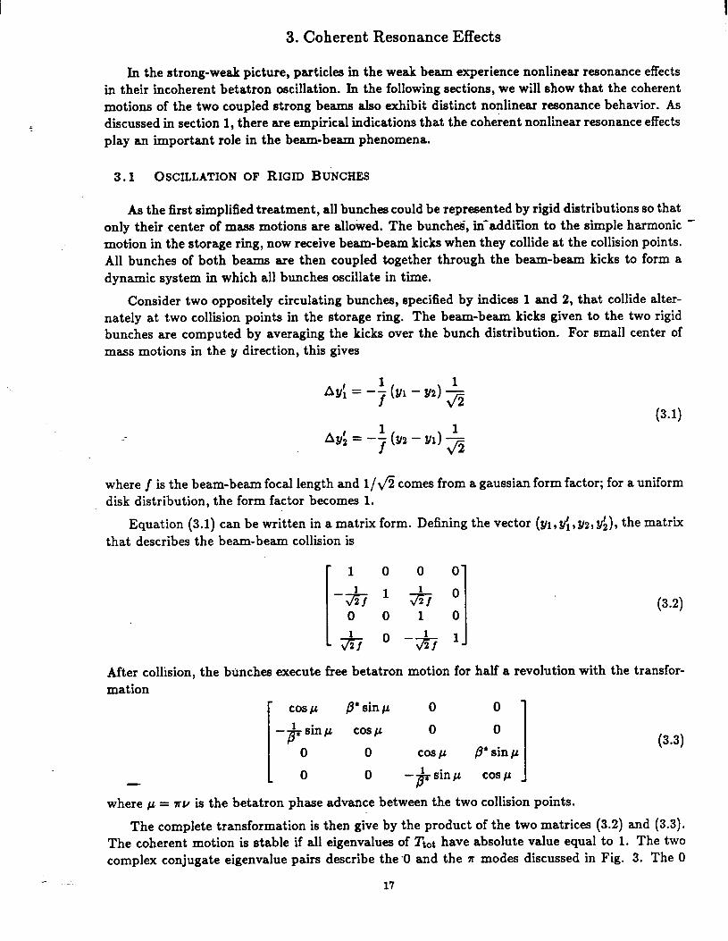
3. Coherent Resonance Effects

In the strong-weak picture, particles in the weak beam experience nonlinear resonance effects in their incoherent betatron oscillation. In the following sections, we will show that the coherent motions of the two coupled strong beams also exhibit distinct nonlinear resonance behavior. As discussed in section 1, there are empirical indications that the coherent nonlinear resonance effects play an important role in the beam-beam phenomena.

3.1 OSCILLATION OF RIGID BUNCHES

As the first simplified treatment, all bunches could be represented by rigid distributions so that only their center of mass motions are allowed. The bunch&, in-addZion to the simple harmonic - motion in the storage ring, now receive beam-beam kicks when they collide at the collision points. All bunches of both beams are then coupled together through the beam-beam kicks to form a dynamic system in which all bunches oscillate in time.

Consider two oppositely circulating bunches, specified by indices 1 and 2, that collide alter- nately at two collision points in the storage ring. The beam-beam kicks given to the two rigid bunches are computed by averaging the kicks over the bunch distribution. For small center of mass motions in the y direction, this gives

. . 44 = -f (Yl - 92) $

(3.1) -- A!& = -f (32 - y1) 5

where f is the beam-beam focal length and l/fi comes from a gaussian form factor; for a uniform disk distribution, the form factor becomes 1.

Equation (3.1) can be written in a matrix form. Defining the vector (~1, y{, 92, yi), the matrix that describes- the beam-beam collision is

1 0 0 0

-& lTi-7 O 0 0 1 0

& O -& l

(3.2)

After collision, the bunches execute free betatron motion for half a revolution with the transfor- mation

cos p /3* sin ~1 0 0

-$rsinj4 co;~ 0 0

0 cos p p’ sin p

0 0 -#

sin p cos p I -

(3.3)

where p = AU is the betatron phase advance between the two collision points.

The complete transformation is then give by the product of the two matrices (3.2) and (3.3). The coherent motion is stable if all eigenvalues of Ttot have absolute value equal to 1. The two complex conjugate eigenvalue pairs describe the ‘0 and the x modes discussed in Fig. 3. The 0

17

0.20 1 I \ ’ I

0.15 - Dipole Mode ‘\ (0)

to

0.10 -

0 0 0.2 0.4 0.6 0.8 1.0

0.20, , , I I I I I Dipole Mode 3Bunchef

0 0.5 I I.5 2 2.5 3 Q-84 “0

0 0.5 1 1.5 2 I I I ’ - Dipole Mode

r4 Bunches s \(d)

I -

0 I 2 3 4 vO 4886A 1

Fig. 15. Stability diagram in (uo, (00) space, where uc is the unperturbed tune for the storage ring and (0 is the beam-beam strength parameter, for the cases with 1, 2, 3 and 4 bunches per beam. The beam bunches are regarded as rigid allowing only dipole coherent motions.

mode is always stable, while the z mode is stable only if

(<L cot 11 . 2Jz7r 2

This stability condition is fi times more stringent than the linearized strong-weak stability condition. This is more clearly seen in the sawtooth diagram Fig. 15(a).

The picture becomes more complicated, although still straightforward, if there are more than one bunch per beam. For instance, when there are B bunches per beam, there will be 2B modes of coherent rigid bunch modes. The stability region is obtained by requiring all 2B modes be stable. Figures 15(b)-(d) h s ows the stability diagrams for the cases with 2,3 and 4 bunches per beam. It is clear that in these multiple-bunch cases, the coherent stability becomes increasingly more stringent than the corresponding incoherent stability condition as given by the dotted lines. The rigid bunch coherent instabilities are most serious when the unperturbed betatron tune u of the storage ring is close to an integer, as seen from Fig. 15. In the next section we will show that the coherent instabilities in general occur when u is close to a rational number.

3.2 HIGHER ORDER BEAM-BEAM MODES

If we relax the condition that all bunches are rigid, the analysis becomes much more com- plicated. Each bunch can then be described only as a superposition of modes in its transverse distribution. The lowest of such modes is the dipole center-of-mass mode just discussed. Then there will have to be quadrupole mode, sextupole mode,etc. The coherent quadrupole mode will be unstable if u is close to n/2; the sextupole mode is unstable near u = n/3.

Figure 16 is an illustration of a coherent beam-beam instability mechanism when u % n/4. Figure 16(a) gives the phase space distributions of the two beams in equilibrium. An infinitesimal

18

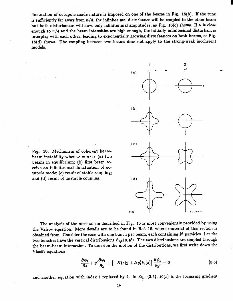
fluctuation of octupole mode nature is imposed on one of the beams in Fig. 16(b). If the tune is sufficiently far away from n/4, the infinitesimal disturbance will be coupled to the other beam but both disturbances will have only infinitesimal amplitudes, as Fig. 16(c) shows. If u is close enough to n/4 and the beam intensities are high enough, the initially infinitesimal disturbances interplay with each other, leading to exponentially growing disturbances on both beams, as Fig. 16(d) shows. The coupling between two beams does not apply to the strong-weak incoherent models.

Fig. 16. Mechanism of coherent beam- beam instability when u = n/4: (a) two beams in equilibrium; (b) first beam re- ceive an infinitesimal flunctuation of oc- tupole mode; (c) result of stable coupling; and (d) result of unstable coupling.

1 5009A22

The analysis of the mechanism described in Fig. 16 is most conveniently provided by using the Valsov equation. More details are to be found in Ref. 16, where material of this section is obtained from. Consider the case with one bunch per beam, each containing N particles. Let the two bunches have the vertical distributions $r,r(y, y’). The two distributions are coupled through the beam-beam interaction. To describe the motion of the distributions, we first write down the Vlasuv equations

Wl - + ytF + [-K(s)y + AY:&(s)] $ = 0 as

(3.5)

and another equation with index 1 replaced by 2. In Eq. (3.5), K(s) is the focussing gradient

19

function and Ayi,s are the single particle beam-beam kicks given by

4nNr, Ay;,s = --

LdY 7 al WY - 0) 7 &’ ~2,1(mi’)

-00 --oo

with L, the horizontal width of the flat beam and

H&E) = 1 l ifZ>O

-1 ifzco

(3.6)

(3.7)

The job is to find the stability of the coupled partial differential Eqs. (3.5)-(3.7). A complete treatment of the problem is unfortunately extremely difficult.-What we can do is to start with- a steady state- distribution $0 for both beams and study if infinitesimal fluctuations around $0

-will result in exponentially growing deviations. From such treatment, we can tell if $0 is stable or not and find the corresponding stability conditions.

To proceed, we define

+1,2 = $0 + &h,2 (3.8) with infinitesimal A$J’s. We then substitute (3.8) into the Vlasov Equations (3.5) and keep only the first order terms in Ati’s. The result is a set of linearized equations

00 co

.- X /

& K(Y -8) /

4l’ f*(Y,c) = 0

-CO -03

(3-g)

where we have made a change of coordinates from (y, y’) to (J,$) according to Eq. (2.7) and we have defined

f* = Ad1 f A+2 (3.10)

Note that the + mode and the - mode are decoupled. Note also that the unperturbed distribution is necessarily a function only of J and that the betatron function used in the transformation has taken into account of the dynamic /3 effect imposed by the unperturbed distribution T/JO.

The linearized Eq. (3.9) is still rather difficult to solve. To illustrate the dynamic behavior of the beam-beam system, however, it suffices to make a model of &, which allows particularly simple mathematical manipulations. The model we use is the water-bag model defined by

+0(J) = ; H (f - J)

where H(s) = 1 if z > 0 and H(z) = 0 if z < 0, and c is the vertical emittance of the equilibrium beam distribution.

The advantage of the water-bag model is that the J dependence of Eq. (3.9) can be easily solved. By inspection, the solutions are

- f*(J,As) = 6 (J - f) cg,‘(s) eic4 L

(3.12)

The 6(J - c/2) factor represents the fact that the perturbations occur only at the edge of the water-bag. We have decomposed the angular part into Fourier components. For simplicity we will drop the + and - superscripts on the g’s.

- 20

Substituting (3.12) into (3.9) g’ Ives an infinite set of equations for the g functions

(3.13)

where we have defined a matrix M with elements

2r 2r

M&k = dcj c /

-W sin 4 /

d6 HI (cos 4 - cos 4) eikB 0 0

(3.14) 32it ife+k=evea =

{ [(L+k)a-I][(&-k)“-l]

- 0 ifL+k=odd

Equation (3.13) * 1 1s inear in the g-functions, allowing it to be solved by matrix techniques. Between collisions, the different g’s are decoupled. A particular g transforms by

with ~1 the integrated betatron phase between collision points. If we define a column vector G for the gl’s,

G=

_ . . .

92

91

90

9-l

g-2 . . .

The transformation matrix between collision points reads

R=

while the beam-beam collision is described by the transformation matrix

- T=If-

(3.15)

(3.16)

(3.17)

where I is the identity matrix. The total transformation Ttot is then the product of (3.17) and (3.18). The stability of the system requires all eigenvalues of the total matrix to have absolute value of unity.

21

In the absence of beam-beam perturbations, the eigenvalues are

x = e-tip ( L=O,fl,f2,... (3.19)

corresponding to the motion of the tih Fourier component of the distribution. The system is of course stable. As the beam-beam strength is increased, the eigenvalues are more and more perturbed until one of the eigenvalues acquires an absolute value larger than 1 and the system becomes unstable.

The coherent instability is most pronounced when the tune is close to a rational number

Near this resonance condition, the Fourier components thatperturb The beam motion most are - gl and g-l. Keeping only those elements in the transformation matrices Ttot we obtain

(1 f ia) e-i2rLA f;ae-i2dA

Ttot = -+iaei2dA (1 F icu)eiZwLA I

where we have defined

The eigenvalues of Ttot satisfies

(3.21)

(3.22)

X2 - 2X (cos 27rtA f Q sin 27reA] + 1 = 0 . (3.23)

One of the eigenvalues has absolute value larger than unity and therefore the system is unstable

jcos2rtA f osin2nlAj > 1 . (3.24)

The “+” and y-n signs refer to the I+ and f- modes. Equation (3.24) determines the instability region near the resonance Y = m/e with a resonance

stop band width approximately given by

1 32 but fit - ’ -

2?r 4@ - 1 c

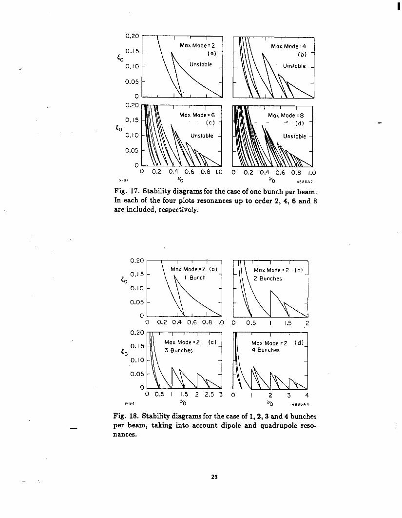
where [ is the beam-beam strength parameter. Figure 17 shows the stability diagrams for the case of one bunch per beam. The eth order

resonance shows up as an unstable region that originates from the tune value u = m/l in these diagrams. In making Fig. 17, numerical results rather than Eq. (3.24) are used. As the matrix is truncated to higher and higher dimension, thus higher and higher resonance orders are included, the stability diagrams become more and more complicated. These numerical results agree quite well with the approximate expression (3.24).

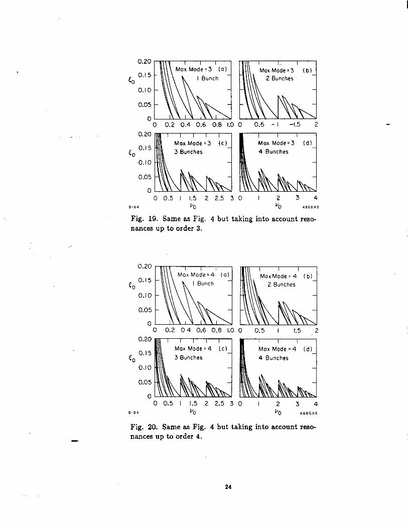
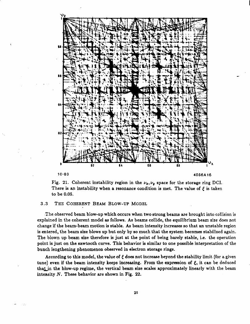
So far we have studied the case with one bunch per beam. For multiple bunches per beam, more book-keeping is needed but the analysis is straightforward. Figures 18, 19 and 20 are the results. According to these results, the coherent instability can indeed play an important role in the beam-beam phenomenon. The analysis does not have to be one-dimensional as assumed so far. Figure 21 gives the results for the case of DC1 in the two-dimensional (uz, uY) space. Again the nonlinear resonance structure is apparent.

- 22

Max Mode = 2

0 0 0.2 0.4 0.6 0.8 1.0

9-84 "0 0 0.2 0.4 0.6 0.8 1.0

uO 4686A2

-

Fig. 17. Stability diagrams for the case of one bunch per beam. In each of the four plots resonances up to order 2, 4, 6 and 8 are included, respectively.

0.20 I I I n , 5 L \ L.-. ..-A--2 (o)

\ NIOX WlOOe = Mox Mode =2 (b)

EO “.l u

0.10 -

0.05 -

0 I 0 0.2 0.4 0.6 0.8 1.0 0 0.5 I 1.5 2

0.20

0.1 5 <O

0.10

0.05

0 0 0.5 I 1.5 2 2.5 3 0 l 2 3 4

9-84 VO “0 4806A4

Fig. 18. Stability diagrams for the case of 1,2,3 and 4 bunches per beam, taking into account dipole and quadrupole reso-

-

nances.

23

0 0 0.2 0.4 0.6 0.8 1.0

- 0.20 Mox Mode =3

0.15 (c)

<O 0.10

0.05

0 0 0.5 I 1.5 2 2.5 3

9-84 UO

MaxMode= (b)

0 053 - I A.5

Max Mode=3 (d)

0 I 2 3 4 UO 4806A5

Fig. 19. Same as Fig. 4 but taking into account reso- nances up to order 3.

0.05

0 0 0.5 I 1.5 2 2.5 3

9-84 VO

0 I 2 3 4 “0 4886A6

-

Fig. 20. Same as Fig. 4 but taking into account res+ nances up to order 4.

24

11 0’4 ’ d.6 ’ d6 ’ I ‘VX

lo-83 4056A 16

Fig. 21. Coherent instability region in the uZ,uY space for the storage ring DCI. There is an instability when a resonance condition is met. The value of 6 is taken to be 0.05.

3.3 THE COHERENT BEAM BLOW-UP MODEL

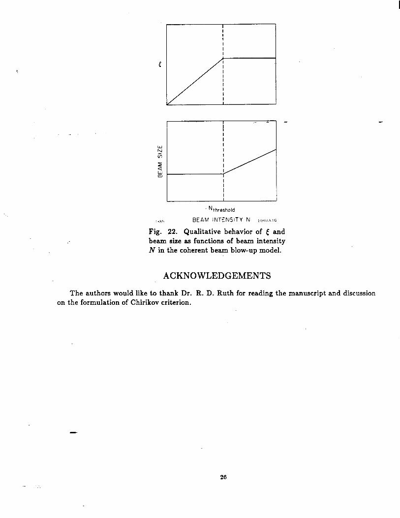
-The observed beam blow-up which occurs when two strong beams are brought into collision is explained in the coherent model as follows. As beams collide, the equilibrium beam size does not change if the beam-beam motion is stable. As beam intensity increases so that an unstable region is entered, the beam size blows up but only by so much that the system becomes stabilized again. The blown up beam size therefore is just at the point of being barely stable, i.e. the operation point is just on the sawtooth curve. This behavior is similar to one possible interpretation of the bunch lengthening phenomenon observed in electron storage rings.

According to this model, the value of e does not increase beyond the stability limit (for a given tune) even if the beam intensity keeps increasing. From the expression of e, it can be deduced thatJn the blow-up regime, the vertical beam size scales approximately linearly with the beam intensity N. These behavior are shown in Fig. 22.

25

-

I-H!? BEAM INTENSITY N 5001~A16

Fig. 22. Qualitative behavior of ( and beam size as functions of beam intensity N in the coherent beam blow-up model.

ACKNOWLEDGEMENTS

The authors would like to thank Dr. R. D. Ruth for reading the manuscript and discussion on the formulation of Chirikov criterion.

-

26 -

REFERENCES

1. H. Zyngier, in “Nonlinear Dynamics and the Beam-Beam Interactions,” AIP Conf. Proc. 57, 1979, p. 137.

2. A. Piwinski, AIP Conf. Proc. 57, 1979, p. 115.

3. J. Le Duff and M. P. Level, Orsay Internal Report, LALRT/8&03,1980.

4. J. Le Duff et al., Proc. XIth International Conference on High Energy Accelerators, 1980, p. 707.

5. A. Chao, AIP Conf. Proc. 57, 1979, p. 42.

6. P. Bambade, Ph.D. Thesis, LAL 84/21,1984. Y - s

71 S. Kheifets, PETRA Note 119, 1976.

8. K. Takayama, Lett. Al Nuovo Cimento, Vol. 34, No. 7 (1982) 190.

9. E. D. Courant and H. S. Snyder, Theory of the Alternating-Gradient Synchrotron, Ann. of Phys. 3 (1958) 1.

10. A. Chao, The Beam-Beam htabilit~, SLAC-PUB-3179,1983.

11. B. Montague, Nucl. Instrum. Methods 187 (1981) 335. 12. G. Zaslavsky and B. Chirikov, Dokl. Akad. Nauk. SSR 169 (1964) 306.

13. F. M. Izraelev, Nearly Linear Mappings and Their Applications, Physica 1D (1980) 243.

14. E. Keil, CERN/ISR-TH/72-25, 1972. . 15; L. Evans, The Beam-Beam Interaction, CERN SPS 183-38, 1983.

16. A. Chao and R. Ruth, Collective Beam-Beam Interaction in Colliding-Beam Storage Ring, Part. Accel. Vol. 16, No. 4, (1985) 201.

-

27