nonlinear beltrami equations
TRANSCRIPT

NONLINEAR BELTRAMI EQUATIONS
Uniqueness and QC FamiliesJarmo Jääskeläinen <[email protected]>
W4: Quasiconformal Geometry and Elliptic PDEsMay 21, 2013 @ IPAM
WITHKari Astala
Daniel Faraco
Albert Clop
László Székelyhidi Jr.

QUASICONFORMAL MAPPING
Infinitesimally quasiconformal functions map disks into ellipsoids.
Homeomorphism is K-quasiconformal if for almost everywhere the classical Beltrami equation holds
2@z
f(z) = @
x
f(z) + i@
y
f(z), 2@z
f(z) = @
x
f(z)� i@
y
f(z), z = x+ iy
@zf(z) = µ(z) @zf(z), |µ(z)| 6 k < 1, K =1 + k
1� k
f : ⌦ ! C 2 W 1,2loc
(⌦)
Cauchy-R
iemann
formal adjoint

One can measurably preassign the eccentricity and angle of the ellipses.
@zf(z) = µ(z) @zf(z), |µ(z)| 6 k < 1, K =1 + k
1� k
Every solution can be factorized as where is analytic and is a homeomorphic solution (Stoïlow factorization).
hg = h � fg 2 W 1,2loc
(⌦)f
major axis
minor axis
=
|@z f |+ |@z f ||@z f |� |@z f |
K

QUASICONFORMAL FAMILYHomeomorphic solution is called normalized if
There is a unique homeomorphic solution that maps ;namely,
is a -linear family of quasiconformal maps (and constant )
Conversely, if one has a -linear family of quasiconformal maps ,
@zf(z) = µ(z) @zf(z)
�(0) = 0,�(1) = 1� : C ! C 2 W 1,2
loc
(C)
0 7! 0, 1 7! a 2 C \ {0}a�(z)
{a�(z) : a 2 C} C 0
the family is generated by one function, f,, (injectivity)
by Stoïlow, solution = (analytic o homeomorphism)
C {a f : a 2 C}
µ(z) =@zf(z)
@zf(z)
@zf(z) 6= 0
one can associate to it a classical Beltrami equation, by setting
It is well-defined (and unique), since almost everywhere.

Families appear in the context of G-convergence properties of -linear Beltrami operators,
Giannetti, Iwaniec, Kovalev, Moscariello, and Sbordone (2004), Bojarski, D’Onofrio, Iwaniec, and Sbordone (2005)
Homeomorphic solutions to -linear Beltrami equation
form an -linear family of quasiregular mappings. Is their linear combination injective?
@zf(z) = µ(z) @zf(z) + ⌫(z) @zf(z), |µ(z)|+ |⌫(z)| k < 1
R
@z � µj(z)@z � ⌫j(z)@z, |µj(z)|+ |⌫j(z)| 6 k < 1
R
R

Yes (after normalization): Homeomorphic solution is uniquely defined knowing its values at two distinct points. Moreover, the linear combination is either homeomorphism or constant.
Homeomorphic solutions to -linear Beltrami equation
form an -linear family of quasiregular mappings. Is their linear combination injective?
@zf(z) = µ(z) @zf(z) + ⌫(z) @zf(z), |µ(z)|+ |⌫(z)| k < 1
R
R
If we normalize , the linear independence of implies that is K-quasiconformal, and we have an -linear family of quasiconformal mappings.
Idea: , where homeomorphism solves a reduced equation
The only homeomorphic solution to the reduced equation that fixes two points is the identity, Astala, Iwaniec, and Martin (2009):
= F � � F
@zf(z) = �(z) Im(@zf(z)) |�(z)| 6 2k/(1 + k2)
z 7! f(z)� tz
1� t�(0) = 0 = (0) �(1), (1)
↵�(z) + � (z), ↵,� 2 R,R

-LINEAR FAMILY OF QC MAPSConversely, if we have an -linear family of quasiconformal mappings
can we define and so that every mapping of the linear family solves the -linear equation given by ?
R
{↵�(z) + � (z) : ↵,� 2 R}R
µ ⌫µ, ⌫R
@zf(z) = µ(z) @zf(z) + ⌫(z) @zf(z)
Yes we can! generated by two mappings (injectivity)
@z�(z) = µ(z) @z�(z) + ⌫(z) @z�(z)@z (z) = µ(z) @z (z) + ⌫(z) @z (z)
µ(z) = i z�z � z�z
2Im(�z z)⌫(z) = i
�z z � �z z
2Im(�z z)
when matrix of the system of linear equations is invertible
On the singular set, we set .Giannetti, Iwaniec, Kovalev, Moscariello, and Sbordone (2004), Bojarski, D’Onofrio, Iwaniec, and Sbordone (2005)
⌫ ⌘ 0

-LINEAR FAMILY OF QC MAPSConversely, if we have an -linear family of quasiconformal mappings
we define
R
{↵�(z) + � (z) : ↵,� 2 R}R
@zf(z) = µ(z) @zf(z) + ⌫(z) @zf(z)
Unique? Yes, by a Wronsky-type theorem, Alessandrini and Nesi (2009), Astala and Jääskeläinen (2009); Bojarski, D’Onofrio, Iwaniec, and Sbordone (2005)
µ(z) = i z�z � z�z
2Im(�z z)⌫(z) = i
�z z � �z z
2Im(�z z)
k < 1/2
Theorem. Suppose are homeomorphic solutions to
for almost every . Solutions and are -linearly independent if and only if complex gradients and are pointwise independent almost everywhere, i.e.,
�, 2 W 1,2loc
(⌦)
@zf(z) = µ(z) @zf(z) + ⌫(z) @zf(z), |µ(z)|+ |⌫(z)| 6 k < 1,
z 2 ⌦
Im(@z� @z ) 6= 0
@z� @z � R
does not change sign, BDIS(2005)

-LINEAR FAMILY OF QR MAPSR@zf(z) = µ(z) @zf(z) + ⌫(z) @zf(z)
Wronsky-type theorem, Alessandrini and Nesi (2009), Astala and Jääskeläinen (2009); Bojarski, D’Onofrio, Iwaniec, and Sbordone (2005)
Jääskeläinen (2012)
k < 1/2
Theorem. Suppose are homeomorphic solutions to
for almost every . Solutions and are -linearly independent if and only if complex gradients and are pointwise independent almost everywhere, i.e.,
�, 2 W 1,2loc
(⌦)
@zf(z) = µ(z) @zf(z) + ⌫(z) @zf(z), |µ(z)|+ |⌫(z)| 6 k < 1,
z 2 ⌦
Im(@z� @z ) 6= 0
@z� @z � R

-linear -linear NonlinearRC
fz = H(z, fz)fz = µ(z) fz + ⌫(z) fzfz = µ(z) fz
measurable -Lipschitz
H(z, w) : C⇥ C ! C
z 7! H(z, w)w 7! H(z, w)
H(z, 0) ⌘ 0k
Difference of two solutions is K-quasiregular
Constants are solutions.
|@zf(z)� @zg(z)| = |H(z, @zf(z))�H(z, @zg(z))| 6 k|@zf(z)� @zg(z)|
BELTRAMI EQUATIONS

-linear -linear NonlinearRC
fz = H(z, fz)fz = µ(z) fz + ⌫(z) fzfz = µ(z) fz
z 7! H(z, w)
There is a unique homeomorphic solution such that ��(0) = 0,�(1) = 1
Theorem. If then the nonlinear equation
admits a unique homeomorphic solution normalized by .
Furthermore, the bound on is sharp.
lim sup|z|!1
k(z) < 3� 2p2 = 0.17157...,
@zf(z) = H(z, @zf(z))
� : C ! C 2 W 1,2loc
(C)�(0) = 0,�(1) = 1
k
There is a unique homeomorphic solution such that ��(0) = 0,�(1) = 1
measurable -Lipschitzw 7! H(z, w) H(z, 0) ⌘ 0k
Not unique in general, Astala, Clop, Faraco, Jääskeläinen, and Székelyhidi Jr. (2012)

z 7! H(z, w)
Theorem. If then the nonlinear equation
admits a unique homeomorphic solution normalized by .
Furthermore, the bound on is sharp.
lim sup|z|!1
k(z) < 3� 2p2 = 0.17157...,
@zf(z) = H(z, @zf(z))
� : C ! C 2 W 1,2loc
(C)�(0) = 0,�(1) = 1
k
measurable -Lipschitzw 7! H(z, w) H(z, 0) ⌘ 0k
Astala, Clop, Faraco, Jääskeläinen, and Székelyhidi Jr. (2012)COUNTEREXAMPLES
ft(z) =
((1 + t) z|z|
p2�1 � t(z|z|1/
p2�1
)
2, for |z| > 1,
(1 + t) z � tz2, for |z| 1,
gt(z) =
((1 + t) z|z|
p2�1 � tz|z|1/
p2�1, for |z| > 1,
z, for |z| 1.
K =1 + k
1� k=
p2 , k = 3� 2
p2

ft(z) =
((1 + t) z|z|
p2�1 � t(z|z|1/
p2�1
)
2, for |z| > 1,
(1 + t) z � tz2, for |z| 1,
gt(z) =
((1 + t) z|z|
p2�1 � tz|z|1/
p2�1, for |z| > 1,
z, for |z| 1.

-linear -linear NonlinearRC
fz = H(z, fz)fz = µ(z) fz + ⌫(z) fzfz = µ(z) fz
There is a unique homeomorphic solution such that ��(0) = 0,�(1) = 1
There is a unique homeomorphic solution such that ��(0) = 0,�(1) = 1
There is a unique homeomorphic solution such that when near the infinity
��(0) = 0,�(1) = 1
k(z) < 3� 2p2
Homeomorphic solution is uniquely defined by its values at two distinct points. Difference is homeomorphism or constant.
{�a : �a K � qc, 0 7! 0, 1 7! a}
-linear family of quasiconformal mappings
-linear family of quasiconformal mappings
family of quasiconformal mappings
C R

{�a : �a K � qc, 0 7! 0, 1 7! a}
-linear family of quasiconformal mappings
-linear family of quasiconformal mappings
family of quasiconformal mappings
C R
FROM FAMILY TO EQUATION
{↵�(z) + � (z) : ↵,� 2 R}{a�(z) : a 2 C}
�(0) = 0,�(1) = 1 �(0) = 0,�(1) = 1
(0) = 0, (1) = i
unique and s.t. every mapping of the family solves the Beltrami equation (Wronsky-type theorem)
µ ⌫
fz = µ(z) fz + ⌫(z) fzfz = µ(z) fz ?fz = H(z, fz)¿
linearly independent, thus their complex gradients are linearly independent

{�a : �a K � qc, 0 7! 0, 1 7! a}We have a family of quasiconformal mappings ,
HOW TO DEFINE EQUATION?
�a(z)� �b(z) is K-quasiconformal.
measurable -Lipschitzz 7! H(z, w)w 7! H(z, w)
H(z, 0) ⌘ 0k
We want nonlinear equation @zf(z) = H(z, @zf(z))
@z�a(z) = H(z, @z�a(z))
|@z�a(z)� @z�b(z)| 6 k|@z�a(z)� @z�b(z)|
Define pointwise
One can extend to whole plane as a Lipschitz map by Kirszbraun extension theorem. Hence there exists a nonlinear Beltrami equation.
Not overdetermined:
w 7! H(z, w)
Unique, when one has a full range for almost every . In the case of linear families
{@z�a(z) : a 2 C} = C{a @z�(z)}, {↵@z�(z) + � @z (z)}
complex gradients are linearly independent (Wronsky-type theorem)
z

{�a : �a K � qc, 0 7! 0, 1 7! a}We have a family of quasiconformal mappings ,
PROPERTIES OF THE FAMILY
�a(z)� �b(z) is K-quasiconformal.
It turns out that exists for almost every (exceptional set might depend on ; and this causes difficulties). Note that exists for almost every (by quasiconformality). The exceptional set depends on .
@zf(z) = H(z, @zf(z))What more can we say about the family, if we know more about the nonlinear Beltrami equation ?
We need some relation between and .
What other properties does the family have? For instance, when do we have a full range for almost every ?{@z�a(z) : a 2 C} = C z
a 7! @a�a(z) az z 7! @z�a(z)
az
za
Astala, Clop, Faraco, and Jääskeläinen

{�a : �a K � qc, 0 7! 0, 1 7! a}�a(z)� �b(z) is K-quasiconformal. measurable z 7! H(z, w)
w 7! H(z, w)
H(z, 0) ⌘ 0
@zf(z) = H(z, @zf(z))
Theorem. For each fixed , the mapping is continuously differentiable. Further, the convergence of derivatives is locally uniform in .
In fact, the directional derivatives
are quasiconformal mappings of all satisfying the same -linear Beltrami equation
k(z) < 3� 2p2 near the infinity -Lipschitz,k
C1
takes care of the first exceptional setz 2 C a 7! �a(z)
@a�a(z)z
@ae�a(z) := lim
t!0+
�a+te(z)� �a(z)
t, e 2 C,
z
@zf(z) = µa(z)@zf(z) + ⌫a(z)@zf(z)
µa(z) = @wH�z, @z�a(z)
�, ⌫a(z) = @wH
�z, @z�a(z)
�
R
Astala, Clop, Faraco, and Jääskeläinen

{�a : �a K � qc, 0 7! 0, 1 7! a}�a(z)� �b(z) is K-quasiconformal. measurable z 7! H(z, w)
w 7! H(z, w)
H(z, 0) ⌘ 0
@zf(z) = H(z, @zf(z))
k(z) < 3� 2p2 near the infinity -Lipschitz,k
C1
takes care of the second exceptional set
Astala, Clop, Faraco, and Jääskeläinen:
Schauder estimates: �a 2 C1,↵loc
(C)
Fixing , Jacobian of
Hence is locally injective (locally homeomorphic, by invariance of domain); in particular, an open mapping.
z
J(a, a 7! @z�a(z)) = Im(@z[@a1�a(z)] @z [@a
i �a(z)]) 6= 0 a.e. z
a 7! @z�a(z)
a 7! @z�a(z) : C ! C
Wronsky-type theorem + Theorem about directional derivatives
C↵loc

{�a : �a K � qc, 0 7! 0, 1 7! a}�a(z)� �b(z) is K-quasiconformal. measurable z 7! H(z, w)
w 7! H(z, w)
H(z, 0) ⌘ 0
@zf(z) = H(z, @zf(z))
k(z) < 3� 2p2 near the infinity -Lipschitz,k
C1
takes care of the second exceptional set
Astala, Clop, Faraco, and Jääskeläinen:
Schauder estimates: �a 2 C1,↵loc
(C)
Fixing , Jacobian of
Hence is locally injective (locally homeomorphic, by invariance of domain); in particular, an open mapping. Can be extended as a continuous mapping between Riemann spheres . Thus ‘the covering map stuff ’ gives that is actually a homeomorphism for almost every . (We get more than the full range .)
z
J(a, a 7! @z�a(z)) = Im(@z[@a1�a(z)] @z [@a
i �a(z)]) 6= 0 a.e. z
a 7! @z�a(z)
a 7! @z�a(z) : C ! CC
z
a 7! @z�a(z) : C ! C
Wronsky-type theorem + Theorem about directional derivatives
C↵loc
{@z�a(z) : a 2 C} = C
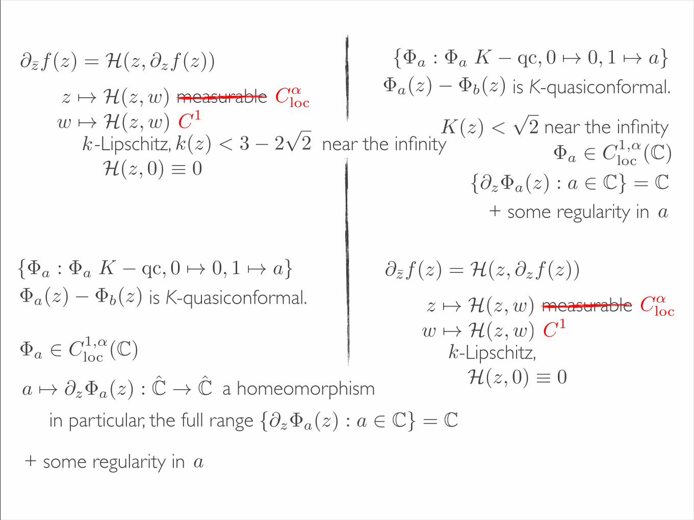
{�a : �a K � qc, 0 7! 0, 1 7! a}�a(z)� �b(z) is K-quasiconformal. measurable z 7! H(z, w)
w 7! H(z, w)
H(z, 0) ⌘ 0
@zf(z) = H(z, @zf(z))
k(z) < 3� 2p2 near the infinity -Lipschitz,k
C1
�a 2 C1,↵loc
(C)
a 7! @z�a(z) : C ! C
C↵loc
{@z�a(z) : a 2 C} = C
{�a : �a K � qc, 0 7! 0, 1 7! a}�a(z)� �b(z) is K-quasiconformal.
a homeomorphismin particular, the full range
+ some regularity in a
�a 2 C1,↵loc
(C){@z�a(z) : a 2 C} = C
+ some regularity in a
measurable z 7! H(z, w)w 7! H(z, w)
H(z, 0) ⌘ 0
@zf(z) = H(z, @zf(z))
-Lipschitz,kC1
C↵loc
K(z) <p2 near the infinity

THANK YOU!