nonlinear dynamic soil-structure interaction in earthquake ... · dssi ssi forces evaluation in the...

DSSI SSI forces evaluation in the time domain Numerical validation Conclusions

Nonlinear Dynamic Soil-StructureInteraction in Earthquake Engineering

Alex Nieto [email protected]

CIFRE contract:ECP Thesis Director: D. Clouteau

EDF R&D / LaMSID Supervisors: N. Greffet, G. Devésa

September 4th 2012LaMSID seminar

1 / 61


Kashiwazaki-Kariwa Nuclear Power Station

7 units; 8 212 MWe∼ Soft soilsInstrumented from 2004

2 / 61


Observed nonlinear behaviour

July 16th, 2007 10:13 AM

Richter Magnitude = 6.8

Depth = 17Km

Hypocenter = 23Km, Epicenter = 16Km

3 / 61


Industrial Context

Periodic seismic risk assessments

Account for nonlinear effects in soil-structure interaction (SSI)calculations

Linear SSI analyses

Efficient BE-FE coupling in the frequency domain

Validated codes: MISS3D and Code_Aster

Goal

Enhance the existing BE-FE so that nonlinearities can beaccounted for within SSI calculations

Avoid full FEM solution (too expensive)

4 / 61


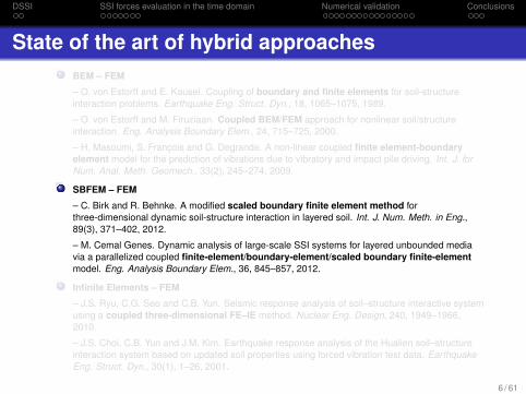
State of the art of hybrid approachesBEM – FEM

– O. von Estorff and E. Kausel. Coupling of boundary and finite elements for soil-structureinteraction problems. Earthquake Eng. Struct. Dyn., 18, 1065–1075, 1989.

– O. von Estorff and M. Firuziaan. Coupled BEM/FEM approach for nonlinear soil/structureinteraction. Eng. Analysis Boundary Elem., 24, 715–725, 2000.

– H. Masoumi, S. François and G. Degrande. A non-linear coupled finite element-boundaryelement model for the prediction of vibrations due to vibratory and impact pile driving. Int. J. forNum. Anal. Meth. Geomech., 33(2), 245–274, 2009.

SBFEM – FEM

– C. Birk and R. Behnke. A modified scaled boundary finite element method forthree-dimensional dynamic soil-structure interaction in layered soil. Int. J. Num. Meth. in Eng.,89(3), 371–402, 2012.

– M. Cemal Genes. Dynamic analysis of large-scale SSI systems for layered unbounded mediavia a parallelized coupled finite-element/boundary-element/scaled boundary finite-elementmodel. Eng. Analysis Boundary Elem., 36, 845–857, 2012.

Infinite Elements – FEM

– J.S. Ryu, C.G. Seo and C.B. Yun. Seismic response analysis of soil–structure interactive systemusing a coupled three-dimensional FE–IE method. Nuclear Eng. Design, 240, 1949–1966,2010.

– J.S. Choi, C.B. Yun and J.M. Kim. Earthquake response analysis of the Hualien soil–structureinteraction system based on updated soil properties using forced vibration test data. EarthquakeEng. Struct. Dyn., 30(1), 1–26, 2001.

5 / 61






SBFEM – FEM






6 / 61






SBFEM – FEM






7 / 61


Summary

1 Dynamic SSI problem

2 SSI forces evaluation in the time domain

3 Numerical validation

4 Conclusions and future work

8 / 61


1 Dynamic SSI problemGeneral resolution strategyInteraction forces: convolution integral




9 / 61


SSI Problem: resolution strategy

DSSI in EE = building + soil + incident seismic field

10 / 61



domain decomposition technique

11 / 61



BEM - FEM coupling = MISS3D - Code_Aster coupling

12 / 61



BEM - FEM coupling = MISS3D - Code_Aster coupling

13 / 61



LINEAR: resolution in frequency domain

NONLINEAR: resolution in time domain

14 / 61


Interaction forces: convolution integral

Assuming linear behaviour and FE discretization (Γ-interface):

−ω2Mu(ω) + iωCu(ω) + Ku(ω) +

[0

Zs(ω)uΓ(ω)

]=

[0

Fs(ω)

]

? ? ? ? ?

Mu(t) + Cu(t) + Ku(t) +

[0

RΓ(t)

]=

[0

Fs(t)

]where

Fs(t): seismic loading,RΓ(t): interaction forces, i.e. the convolution integral:

RΓ(t) = (Z ∗ uΓ)(t) =

∫ t

0Z(τ)uΓ(t − τ) dτ

15 / 61



2 SSI forces evaluation in the time domainNumerical problemsConvolution Quadrature MethodHybrid Laplace-Time domain Approach



16 / 61


Numerical problems

Soil impedance is assumed as [COTTEREAU07]:

Z(ω) = −ω2 M + iω C + K︸︷︷︸singular part

+ Zr(ω)︸︷︷︸regular part

, Zr(ω) −−−−→ω→∞

0

MKCtime domainformulation

17 / 61


Numerical problems




, Zr(ω) −−−−→ω→∞

0

?

12π

∫ +∞

−∞Z(ω) eiωt dω

Cut-offfrequency

Z(t) = M δ(t) + C δ(t) + K δ(t) + Zr(t)

?

Singularkernel


18 / 61


Numerical problems




, Zr(ω) −−−−→ω→∞

0

?

12π

∫ +∞

−∞Z(ω) eiωt dω

Cut-offfrequency

Z(t) = M δ(t) + C δ(t) + K δ(t) + Zr(t)

?

Singularkernel

(Z ∗ u)(t) = M u(t) + C u(t) + K u(t) + (Zr ∗ u)(t)

with (δ(m) ∗ f)(t) = (δ ∗ f (m))(t) = f (m)(t)


19 / 61


Numerical problems




, Zr(ω) −−−−→ω→∞

0

?

12π

∫ +∞

−∞Z(ω) eiωt dω Cut-off

frequency

Z(t) = M δ(t) + C δ(t) + K δ(t) + Zr(t)

?

Singularkernel




20 / 61


Numerical problems




, Zr(ω) −−−−→ω→∞

0

?

12π

∫ +∞


frequency

Z(t) = M δ(t) + C δ(t) + K δ(t)︸︷︷︸distributional character

+ Zr(t)

?

Singularkernel




21 / 61


Numerical problems




, Zr(ω) −−−−→ω→∞

0

?

12π

∫ +∞


frequency

Z(t) = M δ(t) + C δ(t) + K δ(t)︸︷︷︸distributional character

+ Zr(t)

?

Singularkernel

(Z ∗ u)(t) = M u(t) + C u(t) + K u(t) + (Zr ∗ u)(t) MKCtime domainformulation

22 / 61


Cut-off frequencyInverse Discrete Time Laplace transform (closed integration contour)

f(n∆t) =1

2πi

∮C

f(z) z−n−1 dz , z = es∆t ; s ∈ C

Singular convolution kernel

Flexibility formulation[WOLF85, FRANÇOIS08]

Dissipative integrators

u(t) =

∫ t

0F(τ)R(t − τ) dτ , F(t) = F−1Z−1

s (ω)

MKC time formulation

(Z ∗ u)(t) = (ZM ∗ u)(t) + (ZC ∗ u)(t) + (ZK ∗ u)(t)

Approaches based on lumped-parameter models [DEBARROS90]

Time evaluation of the aerodynamic forces in FSI problems [KARPEL82]

Convolution Quadrature Method

||Z(s)|| ≤ M|s|µ , µ,M ∈ RHolomorphic at least on <e(s) > σ0

23 / 61


Cut-off frequencyInverse Discrete Time Laplace transform (closed integration contour)

f(n∆t) =1

2πi

∮C

f(z) z−n−1 dz , z = es∆t ; s ∈ C

Singular convolution kernel

Flexibility formulation[WOLF85, FRANÇOIS08]

Dissipative integrators

u(t) =

∫ t

0F(τ)R(t − τ) dτ , F(t) = F−1Z−1

s (ω)

MKC time formulation


Approaches based on lumped-parameter models [DEBARROS90]

Time evaluation of the aerodynamic forces in FSI problems [KARPEL82]

Convolution Quadrature Method

||Z(s)|| ≤ M|s|µ , µ,M ∈ RHolomorphic at least on <e(s) > σ0

24 / 61


Convolution Quadrature Method [LUBICH88]

The CQM approximates:

(Z ∗ u)(t) =

∫ t

0Z(τ) u(t − τ) dτ , t > 0

by a discrete convolution.

?

Z(t) = L−1 Z(s)s ∈ C

(Z ∗ u)(t) =1

2πi

∫σ+iR

Z(s)∫ t

0e sτu(t − τ) dτ︸︷︷︸

y(t ; s)

ds

y = s y + u , y(0 ; s) = 0 CQM

{Linear multistep methodRunge-Kutta method

25 / 61




(Z ∗ u)(t) =

∫ t

0Z(τ) u(t − τ) dτ , t > 0


?

Z(t) = L−1 Z(s)s ∈ C

(Z ∗ u)(t) =1

2πi

∫σ+iR

Z(s)∫ t


y(t ; s)

ds

y = s y + u , y(0 ; s) = 0 CQM


26 / 61




(Z ∗ u)(t) =

∫ t

0Z(τ) u(t − τ) dτ , t > 0


?

Z(t) = L−1 Z(s)s ∈ C

(Z ∗ u)(t) =1

2πi

∫σ+iR

Z(s)∫ t


y(t ; s)

ds

y = s y + u , y(0 ; s) = 0

CQM


27 / 61




(Z ∗ u)(t) =

∫ t

0Z(τ) u(t − τ) dτ , t > 0


?

Z(t) = L−1 Z(s)s ∈ C

(Z ∗ u)(t) =1

2πi

∫σ+iR

Z(s)∫ t


y(t ; s)

ds

y = s y + u , y(0 ; s) = 0 CQM


28 / 61


Laplace domain discretization

once the ODE is discretized, the following convolution:

(Z ∗ u)(t) =

∫ t

0Z(τ)u(t − τ) dτ , t > 0

is approximated by a discrete convolution (∆t > 0):

(Z ∗ u)(n∆t) =

n∑k=0

Φkun−k , n = 0, 1, ..,N

where Φk are computed by IFFT:

Φk =ρ−n

L

L−1∑l=0

Z (sl) e−i 2πlL n, n = 0, 1, ..,N

29 / 61




(Z ∗ u)(t) =

∫ t

0Z(τ)u(t − τ) dτ , t > 0


(Z ∗ u)(n∆t) =

n∑k=0

Φkun−k , n = 0, 1, ..,N


Φk =ρ−n

L

L−1∑l=0

Z (sl) e−i 2πlL n, n = 0, 1, ..,N

30 / 61




(Z ∗ u)(t) =

∫ t

0Z(τ)u(t − τ) dτ , t > 0


(Z ∗ u)(n∆t) =

n∑k=0

Φkun−k , n = 0, 1, ..,N


Φk =ρ−n

L

L−1∑l=0

Z (sl) e−i 2πlL n, n = 0, 1, ..,N

31 / 61


Backward Differentiation Formula (BDF)

Z (sl) ? sl =r(zl)

∆t

Pth-order BDF(implicit / dissipative):

r(zl) =∑P

k=11k (1− zl)

k

P=2 is considered(<e r(zl) > 0):

r(zl) =32− 2zl +

12

z2l

contours of r(zl), for |zl| = ρ

32 / 61


Hybrid Laplace-Time domain Approach

Recall that an MKC time formulation wants to be obtained:


The integral convolution:

(Z ∗ u)(t) =

∫ t

0Z(τ)u(t − τ) dτ , t > 0

or, by discretizing in time (∆t > 0):

(Z ∗ u)(n∆t) =

n∑k=0

Φkun−k , n = 0, 1, ..,N

33 / 61



Assuming the soil impedance operator in the form of:

Z(s) = Zm(s)(

Ms2 + Cs + K)


(Z ∗ u)(t) =

∫ t

0Z(τ)u(t − τ) dτ , t > 0


(Z ∗ u)(n∆t) =

n∑k=0

Φkun−k , n = 0, 1, ..,N

34 / 61




Z(s) = Zm(s)(

Ms2 + Cs + K)


(Z ∗ u)(t) =

∫ t

0Z(τ)u(t − τ) dτ , t > 0


(Z ∗ u)(n∆t) =

n∑k=0

Φkun−k , n = 0, 1, ..,N

35 / 61




Z(s) = Zm(s)(

Ms2 + Cs + K)

The integral convolution becomes:

(Z ∗ u)(t) = (Zm ∗ Mu)(t) + (Zm ∗ Cu)(t) + (Zm ∗ Ku)(t)


(Z ∗ u)(n∆t) =

n∑k=0

Φkun−k , n = 0, 1, ..,N

36 / 61




Z(s) = Zm(s)(

Ms2 + Cs + K)

The integral convolution becomes:



(Z ∗ u)(n∆t) =

n∑k=0

ΦkMun−k + ΦkCun−k + ΦkKun−k

where Φk are now computed by means of Zm (sl).

37 / 61


Nonlinear dynamic SSI problem

FEM discretization of the time domain variational form (b-building):[Mbb MbΓ

MΓb MΓΓ

] [ub(t)uΓ(t)

]+

[f int

b (u,u, t, ...)f int

Γ (u,u, t, ...)

]+

[0

RΓ(t)

]=

[0

Fs(t)

]If interaction forces RΓ(t) at t = n∆t are decomposed as:

RΓ,n =

n∑k=0

Φn−kMuk + Φn−kCuk + Φn−kKuk

Then, using a (single step) time integration scheme:

RΓ,n = Φ0Mun + Φ0Cun + Φ0Kun︸︷︷︸Time integration operator

+ Γ|(n−1)∆t︸︷︷︸To the right-hand side of equation

that is:

(MΓ + Φ0M)un + (CΓ + Φ0C)un + (KΓ + Φ0K)un = Fs,n−Γ|(n−1)∆t

(Newmark is used in the following)38 / 61




MΓb MΓΓ

] [ub(t)uΓ(t)

]+

[f int


Γ (u,u, t, ...)

]+

[0

RΓ(t)

]=

[0

Fs(t)


RΓ,n =

n∑k=0





that is:






3 Numerical validationNumerical experimentsSemi-industrial application


41 / 61


Numerical experiments

linear and nonlinear analyses (Newmark)

Soil type

Hard/soft/mediumhomogeneous soils

Layered soil withvelocity inversion

Foundation type

Surface/embeddedrigid foundation

Surface flexiblefoundation

Structure modelLumped model

FE building

3SI (NUPECtests)

Linear reference solution: Frequency BE-FE solutionNL reference solution: Transient calculation with analytical soil impedance

42 / 61


Reactor building (I)

RB: ∼ 1100 ddls on the interface

Nonlinear calculation: linear kinematic hardening lawFlexible foundation (60 modes) [BALMES96]Homogeneous soil (analytical expression available)(Z ∗ u)(t) = (ZM ∗ u)(t) + (ZC ∗ u)(t) + (ZK ∗ u)(t)

43 / 61


Reactor building (II)

Top of the RB: HLTA solution - reference solution

4,5 5 5,5

time [s]

-4

-2

0

2

4

Acc

eler

atio

n [

m/s

²]

Acceleration response time-historyzoom at strong shaking instants

εr = 4%

44 / 61


Partial conclusions

MKC formulation


Regular soil profile (velocity increases with depth);surface foundations;gives closer results to the reference solution (linear and nonlinearanalyses);cannot be used for embedded foundations or irregular layeredsoils;whether is used or not, overall good agreement (< 15%);whether is used or not, conservative solutions are obtained.

45 / 61


Semi-industrial application

Goal: validation of the HLTA on a semi-industrialDynamic Soil-Structure Interaction model

SMART numerical modelModel at 1/4 scale;

Shaking table;

Large number of DoF’s(∼ 20 000);

Complex dynamics (torsionaleffects);

Known RC nonlinear model(international benchmark);

No SSI experimental solution.

[Seismic design and best-estimate Methods Assessment for Reinforced concrete buildings

subjected to Torsion and non-linear effects]46 / 61


Nonlinear SMART numerical model

Bending 1 Bending 2 Torsional Pumping

Eigenfrequencies [Hz] 9.0 15.9 31.6 32.3

DKT shell elements (floorsand walls):GLRC_DM [KOECHLIN07]

Multi-fiber Euler beam:1D-La Borderie [LABORDERIE91]

Linear kinematic hardening law

Rigid base slab (4mx4m) +soil→ DSSI calculation

47 / 61


Transient calculationsNonlinear structure + linear soil→ Time domain calculation

Reference solution

Full FEM

Soil: Rayleighdamping

HLTA

Bounded soil:Rayleigh damping

Unbounded soil:Hysteretic damping

HLTA

Surface interface:MKC formulation


Comparison in terms of Response Spectra and structural damage values48 / 61



Reference solution

Full FEM


HLTA



HLTA





FEM reference solution

7 layers (regular profile) + solid bedrock ∼ 330 000 DoF’s

0 500 1000 1500 2000 2500Shear velocity [m/s]

-140

-120

-100

-80

-60

-40

-20

0

z-co

ord

inat

e [m

]

Vertical soil profile(depth to bedrock)

Periodic BC (lateral)

ABC (zero-th paraxialapprox.) (bedrock)

50 / 61


Input motions

0 2 4 6 8 10

time [s]

-3

-2

-1

0

1

2

3

Acc

eler

atio

n [

m/s

²]

x-direction

Time history of free-field accelerogramx-direction

0 20 40 60 80 100

eigenfrequency [Hz]

0

0,2

0,4

0,6

0,8

1

Pse

ud

o-a

ccel

erat

ion

[g

]

x-direction

PSA-XFree-field accelerogram (5% modal damping)

Free-field accelerograms in x, y and z direction

PGA ∼ 0.2g

Full FEM solution→ Deconvolution technique (1D-FE soil column)

51 / 61


Soil damping model

Rayleigh damping C = α1K + α2Mξ = α1

2 ω + α22

1ω

α1 and α2: end-points (black curve);

α1 and α2: average damping (redcurve).

Hysteretic dampingMISS3D uses βs

βs = 2ξ

Different input motions

0 10 20 30 40 50frequency [Hz]

0,02

0,03

0,04

0,05

Modal

dam

pin

g [

-]

Modal damping Rayleigh damping model

0 20 40 60 80 100eigenfrequency [Hz]

0

0,5

1

1,5

2

2,5

3

Pse

ud

o-a

ccel

erat

ion

[m

/s²]

Hysteretic damping

Rayleigh damping

PSA-X (5% modal damping)Rayleigh damping vs. Hysteretic damping (Full FEM)

52 / 61



Reference solution

Full FEM


HLTA (flexible)



HLTA (rigid)





Substructuring approach

SSI interface: ∼ 3600 DoF’s;

240 interface vibration modes(ensures convergence) [BALMES96].

M, K, C identification

Regular soil profile

Surface foundations

Frequency calculation:

Zs(ω) ≈ −ω2M + jωC + K

54 / 61


Nonlinear analysis: PSA comparison

55 / 61


Nonlinear analysis: Damage comparison

ultimate GLRC_DM damage valuesFEM solution (bending) HLTA with bounded soil (bending)

Full FEM HLTA bounded soil (εr) HLTA surface (εr)

Bending damage 0.87 0.83 (4.5%) 0.84 (3.4%)Tensile damage 0.95 0.92 (3.1%) 0.93 (2.1%)

56 / 61


CPU time

CPU time elapsed without using a parallel solver

Nonlinear: 223 000 s

Linear: 200 000 sNonlinear: 129 000 s

Soil impedancecomputation: 105 000 s

Nonlinear: 4 900 s

Soil impedancecomputation: 2 800 s

57 / 61






58 / 61


Conclusions

Dynamic SSI problem considered:

nonlinear FEM domain solved in the time domain;

impedance operator computed by a Laplace domain BEM;

time domain integral convolution as a boundary condition on the interface.

Using CQM allows to:

directly work with the impedance operator instead of its inverse;

use the IFFT algorithm to compute time sequences (closed integrationcontours);

express the convolution integral in terms of inertial, damping and stiffnessquantities.

Good results are obtained for the case of a semi-industrial application:

FEM reference solution;

Response Spectra and damage comparison.

59 / 61


Future/Current work

nonlinear soil surrounding the structure (dams);

performance improvement (parallel computing);

advanced MKC identification algorithms;

test the HLTA with other soil impedance formulations (not BEM);

accuracy improvement (CQM-Runge Kutta);

analytic proof of numerical stability when single and multisteptime integration schemes are coupled.

60 / 61


Thank you for your attentionAny questions?

Alex Nieto [email protected]

CIFRE contract:ECP Thesis Director: D. Clouteau

EDF R&D / LaMSID Supervisors: N. Greffet, G. Devésa

September 4th 2012LaMSID seminar

61 / 61

nonlinear dynamic soil-structure interaction in earthquake ... · dssi ssi forces evaluation in the...

Documents