nonlinear empirical modeling using local pls models
TRANSCRIPT

Nonlinear empirical modeling using local PLS models
Lars Aarhus
August 17, 1994

Abstract
This thesis proposes some new iterative local modeling algorithms for the multivariate
approximation problem (mapping from RP to R). Partial Least Squares Regression (PLS)
is used as the local linear modeling technique. The local models are interpolated by means
of normalized Gaussian weight functions, providing a smooth total nonlinear model. The
algorithms are tested on both arti�cial and real world set of data, yielding good predictions
compared to other linear and nonlinear techniques.

Preface
This thesisa completes my work for the degree Candidatus Scientarum at the Department
of Informatics, University of Oslo. It has been carried out at SINTEF, Oslo during two
years from August 1992 to August 1994. My supervisors have been Tom Kavli, at SINTEF,
and Nils Christophersen, at the Department of Informatics. I thank them both for valuable
guidance and assistance into the world of empirical modeling.
I will also thank Glenn Lines for intense and fruitful discussions, Irene Rødsten, Jon
von Tetzchner Stephenson, and Svein Linge for careful reading of the manuscript and for
correcting my English, Geir Horn and John W. Bothner for helpful hints, and Erik Weyer
for explaining obscure mathematical details. A special thank goes to the library at SINTEF
for providing all necessary literature.
Oslo, August 17, 1994.
Lars Aarhus
aSet in 12pt Times Roman using LATEX. Drawings made with idraw and plots with MATLAB.
i
Contents
Abbreviations vii
Notation index viii
1 Introduction 1
1.1 Motivation : : : : : : : : : : : : : : : : : : : : : : : : : : : : : : : : : : : : 2
1.2 Overview and scope of thesis : : : : : : : : : : : : : : : : : : : : : : : : : : 4
2 Background 5
2.1 Multivariate approximation : : : : : : : : : : : : : : : : : : : : : : : : : : 5
2.1.1 Variables and samples : : : : : : : : : : : : : : : : : : : : : : : : : 6
2.1.2 Properties of f : : : : : : : : : : : : : : : : : : : : : : : : : : : : : 7
2.1.3 Training (�nding f) : : : : : : : : : : : : : : : : : : : : : : : : : : : 8
2.1.4 Testing (validating f) : : : : : : : : : : : : : : : : : : : : : : : : : : 9
2.2 Modeling techniques : : : : : : : : : : : : : : : : : : : : : : : : : : : : : : 11
2.2.1 Multiple Linear Regression : : : : : : : : : : : : : : : : : : : : : : : 12
2.2.2 Linear projection techniques : : : : : : : : : : : : : : : : : : : : : : 12
2.2.3 Nonlinear techniques : : : : : : : : : : : : : : : : : : : : : : : : : : 15
3 Local modeling 21
3.1 Division of input space : : : : : : : : : : : : : : : : : : : : : : : : : : : : : 22
3.2 Validation and termination of modeling algorithm : : : : : : : : : : : : : : 24
3.3 Weighting and interpolation : : : : : : : : : : : : : : : : : : : : : : : : : : 25
3.4 Local type of model and optimization : : : : : : : : : : : : : : : : : : : : : 29
4 Proposed algorithms 31
4.1 General Algorithm 1 : : : : : : : : : : : : : : : : : : : : : : : : : : : : : : 33
4.2 Algorithm 1a : : : : : : : : : : : : : : : : : : : : : : : : : : : : : : : : : : 34
4.3 Algorithm 1b, 1c, and 1d : : : : : : : : : : : : : : : : : : : : : : : : : : : : 39
4.4 Evaluation on simple test examples : : : : : : : : : : : : : : : : : : : : : : 45
4.4.1 Algorithm 1a : : : : : : : : : : : : : : : : : : : : : : : : : : : : : : 46
4.4.2 Algorithm 1b, 1c, and 1d : : : : : : : : : : : : : : : : : : : : : : : : 56
4.5 Evaluation on a more complex test example : : : : : : : : : : : : : : : : : 59
4.6 Other algorithms and modi�cations : : : : : : : : : : : : : : : : : : : : : : 63
5 Case studies 67
5.1 Introduction : : : : : : : : : : : : : : : : : : : : : : : : : : : : : : : : : : : 67
5.2 Organization : : : : : : : : : : : : : : : : : : : : : : : : : : : : : : : : : : 68
ii

5.3 Simulated chemical reactor : : : : : : : : : : : : : : : : : : : : : : : : : : : 70
5.4 Hydraulic robot manipulator : : : : : : : : : : : : : : : : : : : : : : : : : : 71
5.5 NIR spectroscopy : : : : : : : : : : : : : : : : : : : : : : : : : : : : : : : : 73
5.5.1 Water estimation in meat : : : : : : : : : : : : : : : : : : : : : : : 73
5.5.2 Sti�ness estimation in polymer : : : : : : : : : : : : : : : : : : : : 75
5.6 Interpretation of results : : : : : : : : : : : : : : : : : : : : : : : : : : : : 76
6 Discussion 78
6.1 Evaluation : : : : : : : : : : : : : : : : : : : : : : : : : : : : : : : : : : : : 78
6.2 Future work : : : : : : : : : : : : : : : : : : : : : : : : : : : : : : : : : : : 82
7 Conclusions 84
A Implementation 85
B De�nitions 86
B.1 Average correlation : : : : : : : : : : : : : : : : : : : : : : : : : : : : : : : 86
B.2 Sample statistics : : : : : : : : : : : : : : : : : : : : : : : : : : : : : : : : 86
B.3 Distance metrics : : : : : : : : : : : : : : : : : : : : : : : : : : : : : : : : 87
iii

List of Figures
1.1 Simple empirical modeling with 26 observations. (a) The set of data. (b)
Linear regression. (c) Quadratic regression. (d) Smooth local linear regression. 3
2.1 Over�tting. (a) A good �t to noisy data. (b) An over�tted model. : : : : : 9
2.2 Arti�cial neural network with one hidden layer and one output node. : : : 17
2.3 The MARS and ASMOD model structure. : : : : : : : : : : : : : : : : : : 19
3.1 Splitting of the input space into rectangular boxes in the LSA algorithm. : 23
3.2 General evolution of the estimation error (MSEE), and the prediction error
(MSEP), as a function of increasing model complexity. : : : : : : : : : : : 25
3.3 A two dimensional unnormalized Gaussian function. : : : : : : : : : : : : : 26
3.4 Gaussian contour lines for di�erent choices of �. (a) Identity matrix, � = 1.
(b) Diagonal matrix, � = 1. (c) Identity matrix, � = 12. (d) Diagonal
matrix, � = 12. : : : : : : : : : : : : : : : : : : : : : : : : : : : : : : : : : : 28
4.1 General Algorithm 1. : : : : : : : : : : : : : : : : : : : : : : : : : : : : : 33
4.2 Local regions in input subspace, with boundaries and centers. : : : : : : : 36
4.3 Algorithm 1a (Fixed validity functions). : : : : : : : : : : : : : : : : : : 38
4.4 The concept of radius in local modeling (Identity matrix). : : : : : : : : : 39
4.5 Algorithm 1b (Variable validity functions). : : : : : : : : : : : : : : : : : 41
4.6 Algorithm 1c (Overlapping local regions). : : : : : : : : : : : : : : : : : 43
4.7 Algorithm 1d (Hierarchical local regions). : : : : : : : : : : : : : : : : : 44
4.8 The di�erent combinations of error measure and heuristic. : : : : : : : : : 45
4.9 Surface of f1. : : : : : : : : : : : : : : : : : : : : : : : : : : : : : : : : : : 46
4.10 Predicted surface of f1 based on 300 training samples without noise and 10
local models. : : : : : : : : : : : : : : : : : : : : : : : : : : : : : : : : : : 48
4.11 Predicted surface of f1 based on 300 noisy training samples and 8 local models. 48
4.12 The model with lowest minimum RMSEP based on 300 training samples
without noise. (a) Evolution of RMSEP. (b) Distribution of local centers
(x) in weighting space. : : : : : : : : : : : : : : : : : : : : : : : : : : : : : 49
4.13 The model with lowest minimum RMSEP based on 300 noisy training sam-
ples. (a) Evolution of RMSEP. (b) Distribution of local centers (x) in weight-
ing space. : : : : : : : : : : : : : : : : : : : : : : : : : : : : : : : : : : : : 50
4.14 Surface of f2. : : : : : : : : : : : : : : : : : : : : : : : : : : : : : : : : : : 51
4.15 Predicted surface of f2 based on training samples without noise and 8 local
models. : : : : : : : : : : : : : : : : : : : : : : : : : : : : : : : : : : : : : 53
4.16 The model with lowest minimum RMSEP based on training samples without
noise. (a) Evolution of RMSEP. (b) Distribution of local centers (x) in
weighting space. : : : : : : : : : : : : : : : : : : : : : : : : : : : : : : : : : 54
iv

4.17 Weighting of di�erent local models in the model with lowest minimum RMSEP. 54
4.18 Predicted surface of f2 based on noisy training samples and 6 local models. 55
4.19 Large jumps in the evolution of the RMSEP for Algorithm 1c. (a) 300n.
(b) 200n. : : : : : : : : : : : : : : : : : : : : : : : : : : : : : : : : : : : : : 57
4.20 Typical example of prediction error evolution for Algorithm 1d (300n). : 58
4.21 Nonlinear response functions for the three instruments. : : : : : : : : : : : 59
4.22 Estimation plot for linear PLS model. : : : : : : : : : : : : : : : : : : : : : 61
4.23 Estimation plot for local model with lowest minimum RMSEP. : : : : : : : 61
4.24 Possible decompositions based on the training samples. : : : : : : : : : : : 64
5.1 Predicted surface of u based on 7 local models, with � = 12(e2c). : : : : : : 72
5.2 Predicted surface of u based on 7 local models, with � = 14(e2nc). : : : : : 73
v

List of Tables
4.1 RMSEP for di�erent models for approximating f1b. : : : : : : : : : : : : : 47
4.2 RMSEP for di�erent characteristics. : : : : : : : : : : : : : : : : : : : : : : 50
4.3 RMSEP for di�erent models for approximating f2c. : : : : : : : : : : : : : 52
4.4 RMSEP for di�erent models using Algorithm 1bd. : : : : : : : : : : : : : 56
4.5 RMSEP for di�erent models for the spectrometry data sete. : : : : : : : : 60
4.6 RMSEP for di�erent models for approximating f1 (strategy 2)f . : : : : : : 65
4.7 RMSEP for di�erent models for approximating f2 (strategy 2)g. : : : : : : 66
4.8 RMSEP for di�erent strategies. : : : : : : : : : : : : : : : : : : : : : : : : 66
5.1 A rough characterization of the experimental data sets. : : : : : : : : : : : 69
5.2 Comparison of di�erent models for the simulated chemical reactor. : : : : : 70
5.3 Comparison of di�erent models for the hydraulic robot manipulator. : : : : 71
5.4 Comparison of di�erent models for water estimation in meat. : : : : : : : : 74
5.5 Comparison of di�erent models for sti�ness estimation in polymer. : : : : : 75
vi

Abbreviations
ANN Arti�cial Neural Network
ASMOD Adaptive Spline Modeling of Observation Data
BP Back Propagation
CART Classi�cation And Regression Trees
CNLS Connectionist Normalized Linear Spline
CV Cross Validation
FPE Final Prediction Error
GCV Generalized Cross Validation
HSOL Hierarchical Self-Organized Learning
LSA Local Search Algorithm
LWR Locally Weighted Regression
MARS Multivariate Adaptive Regression Splines
MLP MultiLayer Perceptron network
MLR Multiple Linear Regression
MSC Multiplicative Signal Correction
MSE Mean Square Error
MSECV Mean Square Error of Cross Validation
MSEE Mean Square Error of Estimation
MSEP Mean Square Error of Prediction
NARMAX Nonlinear AutoRegressive Moving Average with eXogenous inputs
NIPALS Nonlinear Iterative PArtial Least Squares
NIR Near InfraRed
NRMSEE Normalized Root Mean Square Error of Estimation
NRMSEP Normalized Root Mean Square Error of Prediction
PCA Principal Component Analysis
PCR Principal Component Regression
PLS Partial Least Squares regression
PPR Projection Pursuit Regression
RAN Resource-Allocation Network
RBFN Radial Basis Function Network
RMSEE Root Mean Square Error of Estimation
RMSEP Root Mean Square Error of Prediction
vii
Notation index
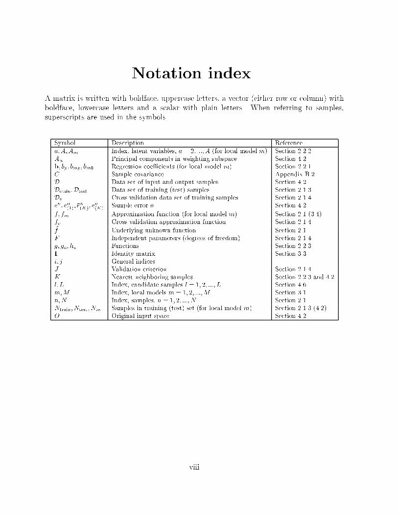
A matrix is written with boldface, uppercase letters, a vector (either row or column) with
boldface, lowercase letters and a scalar with plain letters. When referring to samples,
superscripts are used in the symbols.
Symbol Description Reference
a;A;Am Index, latent variables, a = 2; :::; A (for local model m) Section 2.2.2
Aw Principal components in weighting subspace Section 4.2
b; bp; bmp; bm0 Regression coe�cients (for local model m) Section 2.2.1
C Sample covariance Appendix B.2
D Data set of input and output samples Section 4.2
Dtrain;Dtest Data set of training (test) samples Section 2.1.3
Dv Cross validation data set of training samples Section 2.1.4
en; e
n
(1); en
(K); en
(K) Sample error n Section 4.2
f; fm Approximation function (for local model m) Section 2.1 (3.4)
fv Cross validation approximation function Section 2.1.4�f Underlying unknown function Section 2.1
F Independent parameters (degrees of freedom) Section 2.1.4
g; ga; ha Functions Section 2.2.3
I Identity matrix Section 3.3
i; j General indices
J Validation criterion Section 2.1.4
K Nearest neighboring samples Section 2.2.3 and 4.2
l; L Index, candidate samples l = 1; 2; :::; L Section 4.6
m;M Index, local models m = 1; 2; :::;M Section 3.1
n;N Index, samples, n = 1; 2; :::; N Section 2.1
Ntrain; Ntest; Nm Samples in training (test) set (for local model m) Section 2.1.3 (4.2)
O Original input space Section 4.2
viii

Symbol Description Reference
p; P Index, input variables, p = 1; 2; :::; P Section 1.1
pa Loading column vector in PLS Section 2.2.2
P Covariance matrix of input or latent variables Section 3.3
qa Output loading Section 2.2.2
r Average correlation Appendix B.1
rm; rmax Radius (for local model m) Section 4.3
R Correlation coe�cient matrix of input variables Appendix B.1
sm Splitsample index Section 4.2
S Sample standard deviation Appendix B.2
t Latent variable row vector Section 2.2.2
tn; ti Projected sample row vector n (i) Section 4.2
ta Principal component or score a (column vector) Section 2.2.2
ta Latent variable a Section 2.2.2
T;Ttest Projected input training (test) matrix Section 2.2.2 (4.2)
v; V Index, cross validation subsets v = 1; 2; :::; V Section 2.1.4
vap;va Weights, weight column vector Section 2.2.2
wm Weights (for local model m) Section 3.3
wa Loading weight column vector Section 2.2.2
W Weighting principal component input subspace Section 4.2
x Input variable row vector Section 2.1
xn;xi Input sample row vector n, (i) Section 2.1
xp Input variable column vector p Section 2.1
xp Input variable p Section 2.1
X;Xtest;Xm Input training (test) matrix (for local model m) Section 2.1 (4.2)
y Output variable Section 2.1
yn; y
i Output sample n, (i) Section 2.1
�y Prediction of output variable Section 2.1.4
y;ytest;ym Output training (test) column vector (for local model m) Section 2.1 (4.2)
� Smoothing matrix Section 3.3
�; �m Smoothing parameter (for local model m) Section 3.3
�; �m Center of validity function (for local model m) Section 3.3 and 4.2
�; �m Validity function (for local model m) Section 3.3
ix

1
Introduction
Empirical modelling can be de�ned as the problem of establishing a mathematical model or
description of a system merely from a limited number of observations of di�erent variables
in the system. The model is usually an input/output model where some variables, named
input variables, are used to predict the response of the remaining one(s), named output
variable(s). The system is either static, i.e. is in a �xed condition, or dynamic, i.e. undergoes
an evolution in time.
One example of its use is in the �eld of chemical processing industry, where complicated
chemical processes with unknown relationships between process variables are investigated.
Empirical modelling can then be used to gain insight in these relationships. Other �elds
where empirical modelling is applied today include:
� Chemometrics
� NIR spectroscopy
� Image processing
� Classi�cation
� Control systems
� Geology
� Economy
The main reason for applying empirical modelling in these �elds is because analytical
models, which generally are the most desirable, are either highly inaccurate or very di�cult
to derive. Both is the case when one has very little a priori knowledge about the system.
In these �elds, an analytical model would also be very complex since the number of input
variables is often very high. One is therefore left with the second-best alternative, empirical
modelling, in order to interpret and understand the connections between the variables
involved in the system. This is important since a model based on better understanding
will often lead to a decrease in the error of prediction, and can in the end even reduce
the total expenses of a company, if for instance, the system one is modeling is part of an
industrial process.
1

1 Introduction 2
1.1 Motivation
When doing empirical modeling there are many di�erent techniques and algorithms avail-
able. One common way of classifying them is to separate them into global and local tech-
niques. In a globalmodeling technique the idea is to �nd one function which describes the re-
lationship between the variables. This function will be valid in the whole input domain. Ex-
amples of such techniques are Multiple Linear Regression (MLR) [Johnsen and Wichern 88],
Principal Component Regression (PCR) [Martens and Næs 91], and Partial Least Squares
Regression (PLS) [Wold et al. 84, Geladi and Kowalski 86, Lorber et al. 87, Höskuldsson 88].
The idea in a local modeling scheme is to �nd local functions which only describe the
relationship between the variables in a local domain in the input space. These local mod-
els can then be interpolated, yielding a global description of the system. Local modeling
schemes employ the principle of divide-and-conquer. This principle states that the solution
to a complex problem can be solved by dividing it into smaller independent problems.
These problems are then solved, and their solutions are combined yielding the solution to
the original complex problem. Examples of local techniques are Locally Weighted Regres-
sion (LWR) [Næs et al. 90, Næs and Isaksson 92], Arti�cial Neural Networks (ANN) with
Radial Basis Functions (RBF) [Moody and Darken 88, Stokbro et al. 90], the ASMOD al-
gorithm [Kavli 92] and the LSA algorithm [Johansen and Foss 93]. All the techniques are
treated in greater detail in chapter 2.
To illustrate the idea behind empirical modeling and also the di�erence between global
and local modeling, a simple example is given. Consider the intuitively easiest problem to
solve, namely the static univariate case, i.e. a single input variable, x, and a single output
variable, y. All one is given is N corresponding observations of the two variables. Hence
the problem can be formulated as �nding the best relationship between x and y based on
the N observations. It might be instructive to think of the observations as data points in
a two dimensional space, see �gure 1.1a.
If linearity is assumed in x, the most common solution is to �t a straight line through
the set of data e.g. by the method of least squares. The result is a linear relationship
between x and y, described by the line of regression ,i.e. the slope b and the y-intercept b0.
Thus, the global empirical model is y = b0 + bx, see �gure 1.1b.
However, if the set of data clearly shows a nonlinear behavior, as is the case in this
example, a better approach might be to �t a nonlinear function to the set of data, giving
a nonlinear global empirical model. An example of such is the quadratic model y =
b0+ b1x+ b2x2, where the parameters b0, b1, and b2 are again found by the method of least
squares. The resulting curve on our set of data is given in �gure 1.1c.
Another interesting alternative when solving this nonlinear problem, is to divide the
N observations into a number of di�erent groups based on their value along the x-axis.
By assuming linearity and performing linear regression within each group, local linear
regression models are formed. This approach is an example of local empirical modeling.
The result for our set of data can be seen in �gure 1.1d. Here the number of groups is
3, and the local models are interpolated using a weight function to avoid piecewise linear
functions.

1 Introduction 3
-5 0 5-20
0
20
40
60
80
X
Y
The set of data
-5 0 5-20
0
20
40
60
80
X
Y
Linear regression
-5 0 5-20
0
20
40
60
80
X
Y
Quadratic regression
-5 0 5-20
0
20
40
60
80
X
Y
Smooth local linear regression
Figure 1.1: Simple empirical modeling with 26 observations. (a) The set of data. (b)
Linear regression. (c) Quadratic regression. (d) Smooth local linear regression.
This example can easily be expanded to the multivariate case with P input variables, but
still only a single output variable, i.e. a mapping from RP to R. Apparently this system
is more complex than in the univariate case, but the same kind of thinking concerning
nonlinearity/linearity and global/local models can still be applied. A further expansion to
multiple number of output variables can be done, simply by modeling one y-variable at
a time. The term multivariate system will from now on refer to a system with P input
variables and one output variable.

1 Introduction 4
1.2 Overview and scope of thesis
This thesis presents some new nonlinear empirical modeling algorithms, all based on local
modeling. As seen from the example in section 1.1, the way of thinking that nonlinearity
can be approximated by local linearity is appealing both because it is simple and because
it is not very computationally demanding. The proposed algorithms are all iterative when
it comes to �nding the local models. They are constructed for a general framework, and
are not directed towards any particular application or problem, although emphasis is on
prediction. A nonlinear connection between input and output variables is always assumed.
High dimensional (P > 3), noisy problems are of special interest, especially when the input
variables are correlated.
The rest of the thesis is organized as follows:
� The next chapter takes a closer look at general problems when doing empirical mod-
eling. In addition, some of the most important existing modeling techniques are
presented.
� Chapter 3 covers problems that are speci�c to local modeling.
� In chapter 4, the proposed algorithms and the philosophy behind them are described
and tested on arti�cial examples.
� The results obtained by applying the best of the proposed methods on four well-
known data sets, are given in chapter 5.
� A further discussion on some of the algorithms and an evaluation of their performance
takes place in chapter 6.
� The last chapter contains the main conclusions of the work in this thesis.

2
Background
This chapter provides a general background to empirical modeling, as seen from the multi-
variate approximation point of view [Poggio and Girosi 90]. First, the problem formulation
is speci�ed, and some important aspects which often cause problems in the modeling are
presented. Empirical modeling as a two-step process is then described. The most important
linear techniques, as well as a review of di�erent nonlinear techniques are presented. Local
modeling, which can be seen as a special class within nonlinear modeling, is introduced in
greater detail in chapter 3.
2.1 Multivariate approximation
The general problem treated in this thesis can be formulated as a multivariate approxima-
tion problem. In our context this means �nding the best possible nonlinear relationship
between the vector of input variables, x = (x1; :::; xP ) 2 RP , and the scalar output variable,
y 2 R. The relationship will be of the form
y � �y = f(x) (2.1)
where f is a nonlinear approximation function, and �y is the predicted value of y. This
de�nition is motivated by the assumption that there exists an underlying function, �f , from
which both x and y are generated. Unfortunately, �f is unknown to us.
To help us �nd f , the only information that is available is N di�erent observations, or
samples, of x and y. In other words xn; n = 1; 2; :::; N and yn; n = 1; 2; :::; N . Usually N is
greater than P , but there are situations e.g. in spectrometry where this is not always true.
The data can be arranged in two matrices, denoted X and y. X is a N � P matrix
having x1 to xN as row vectors, whereas y is a N � 1 matrix (column vector) consisting of
y1 to yN . The column vectors of X, i.e. sample values from one input variable, are denoted
xp; p = 1; 2; :::; P .
5

2 Background 6
Another way to formulate the general problem is by trying to visualize the situation
geometrically. All the corresponding samples of x and y can then be thought of as N
geometrical points spread out in a P + 1 dimensional hyperspace, having orthogonal axes
formed by the P + 1 variables. The solution to the problem of identifying f is then the
best P -dimensional hyperplane �tted to all the points, if f is to be globally linear, or more
generally, the best manifold, if one is looking for a nonlinear model.
An important reason why only an approximate, and not an exact relationship can
be found, is because of disturbances or noise in the samples. The presence of noise is
responsible for a number of undesirable phenomena, such as over�tting, outliers, and the
bias/variance problem. The purpose of any approximation function, f , is to �lter away
as much noise as possible, but at the same time to keep the underlying structure in the
system.
2.1.1 Variables and samples
The variables x1,...,xP and y are modelled as stochastic variables corrupted by noise, be-
cause there is always an element of chance in the real world, where no system is completely
deterministic. Hence the description of the variables includes statistical terms such as mean
and variance. However, no assumptions are made about the underlying probability density
functions from which the observations are generated.
Three important aspects of stochastic variables are expected to cause di�culties in the
problem context of this thesis:
Internal correlation. The di�erent input variables are often strongly internally corre-
lated. This might cause problems when using algorithms like MLR, which assumes
that X has full rank i.e. no or insigni�cant collinearity in X. The result is un-
stable parameter values and basis for serious misinterpretations of the model, f
[Dempster et al. 77]. One common way to overcome this problem is to project
the samples in the P -dimensional hyperspace onto a lower dimensional hyperspace
spanned by orthogonal, uncorrelated variables. PCR and PLS are two algorithms
which use this concept of projection.
High dimensionality. When the number of input variables, P , is higher than at least 3,
one talks about a high dimensional set of data, and a corresponding high dimensional
hyperspace of samples. In such a hyperspace things do not behave as nicely as in
a simple two or three dimensional space. One particular problem is that the higher
the dimension, i.e. the larger P is, the more sparsely populated with observation
samples, the hyperspace tends to be. In fact, if the dimension is increased by one,
one needs an exponential growth in the number of samples, N , in order to ensure
the same density, d. (N = dP ) Similarly, the number of parameters required to
specify the model, f , will also increase exponentially with P . This is known as the
curse of dimensionality. To avoid this curse, one could always assure oneself that one
has a su�ciently large number of samples. However, this is an unrealistic approach
since N is a number which is most likely to be �xed. Instead, the solution is either

2 Background 7
to reduce the dimensionality by projections (e.g. PCR and PLS), to decompose the
input variables by expressing f as a sum of lower dimensional combinations of the
input variables (e.g. MARS [Friedman 88] and ASMOD), or to put strong constraints
on the model complexity.
Outliers. Since the variables are corrupted by noise, some of the samples could show
some types of departure from the rest of the data. Such samples are called outliers or
abnormal observations. The question is what to do with samples like these. Should
they simply be removed from the sample collection, or, on the contrary, be regarded as
the most important carriers of information? And on what basis should such a decision
be made? There is no simple solution here, especially not when doing nonlinear
modeling where the di�erence between what is noise and what is a nonlinear trend is
much smaller. Therefore, removal of outliers in nonlinear modeling is more dangerous
than in linear modeling, and should only be done with extreme care.
2.1.2 Properties of f
A solution f , to equation 2.1, should have the following generally desirable properties:
� First of all, f should give an as good as possible prediction, �y, of y when presented
with a new input vector, x. This is the main objective when developing prediction
models.
� Secondly, f should be parsimonious with as few parameters and local models as
possible. This is in accordance with the parsimony principle of data modeling
[Seasholtz and Kowalski 93], which states:
If two models in some way adequately model a given set of data, the one de-
scribed by a fewer number of parameters will have better predictive ability
given new data.
This principle is also known as Occam's razor.
� Lastly, f should be a smooth function. By smooth is meant throughout this thesis
C1. A smooth f will have better generalization properties than discontinuous or
piecewise smooth models [Poggio and Girosi 90], i.e. it will make better predictions
of y. Another reason for requiring smoothness is that the underlying relationship, �f ,
which one is trying to model, is in fact often assumed to be smooth. Hence it appears
only natural that f should be smooth as well.

2 Background 8
2.1.3 Training (�nding f)
The process of �nding f is referred to as the learning or training step of multivariate
approximation. This step consists of �nding both f itself, and the set of parameters in f
which provides the best possible approximation of �f on the set of training samples. These
training samples either equals the N samples previously de�ned or are a subset of these.
The latter is the case if the N samples are divided into disjunct training and test sets.
From now on, the number of training samples is in any case denoted Ntrain. Likewise, the
set of training samples, known as the training set, is denoted Dtrain. The test set, if present,
is denoted Dtest, with the number of test samples denoted by Ntest.
The main problems which immediately occur in the training step are essentially those
of approximation theory and are listed below:
Model structure The determination of the model structure is the �rst and foremost task.
With model structure is meant which function, f , to use in the approximation. Is a
linear f su�cient, or must a nonlinear be used? What one usually does is to start
with a simple linear model, and then try more complex models if the linear approach
was not a good choice. This is known as the representation problem. Determining
the number of layers and nodes in an ANN is an example of this problem.
Model algorithm and parameters Once the model structure is determined, the next
problem is to decide which mathematical algorithm to use to �nd the optimal values
of the parameters for a given f , and then �nding these values. Usually, the choice
of algorithm is guided by the choice of model structure, but sometimes there is no
dependency between algorithm and structure. For instance, MLR, PCR and PLS are
all algorithms that produce linear models in x, just in di�erent ways. Often, these
linear models are not even similar, but they are still all linear. The parameter values
are estimated by the algorithm. In this process the model structure must satisfy
speci�c criteria which put constraints on the parameter values. Such criteria can be
least squares �t, continuity, smoothness etc.
The choice of algorithm and model structure will very much depend on what kind of
problem one is investigating, since no algorithm is universally the best.
Another aspect is the e�ciency of the algorithm. There is only seldom use for an
algorithm which might give very good models, but at a high computational cost, compared
to another which computes f in a fraction of that time and with only slightly worse results
in terms of prediction ability. Examples of the former are di�erent ANN, which are still
slow in comparison with e.g PLS.

2 Background 9
-5 0 5-20
-10
0
10
20
30
40
50
60
70
X
Y
-5 0 5-60
-40
-20
0
20
40
60
80
X
YFigure 2.1: Over�tting. (a) A good �t to noisy data. (b) An over�tted model.
2.1.4 Testing (validating f)
Once the training step is over and a new model, f , is derived, the second important step
in empirical modeling can start. This step is referred to as the validation or testing step,
and consists of validating f against certain requirements. Whether or not f meets these
requirements will decide whether f is a good model for our purpose or not. Usually one is
interested in the predictive ability of f on new input samples, x. Such a requirement can
be speci�ed in terms of a validation criterion.
One reason for validating f is to avoid over�tting, i.e. modeling of noise as well as
underlying structure. The problem of over�tting happens when too much e�ort is put into
�tting f to the training set. An illustration of an over�tted model and another which is not,
on the same training set, is given in �gure 2.1. The over�tted model in fact interpolates
between the training samples because too many free parameters are allowed in f . The
result of over�tting is a much worse prediction ability on new input samples. Since an
over�tted model attempts to model both the noise and the system, over�tting is more
likely to happen the more noise is present in the samples. For a system without noise,
over�tting will generally not be a problem.
Since one wants to measure the generalization properties, the ideal validation criterion
would be to minimize the expected mean square error (MSE) between the `true' output,
y, and the predicted output, �y given by
J�
MSE = E
h(y � �y)
2i
(2.2)
However, minimizing J�
MSE can not be done analytically since the probability density
functions for the variables are unknown. An estimate of J�MSE must therefore be minimized.

2 Background 10
Several such estimators exist, the most used is the empirical mean square error de�ned by
JMSE =1
N
NXn=1
(yn � �yn)2
(2.3)
A very tempting approach is to use the Ntrain samples in the training set in the com-
putation of JMSE. The estimator is then known as the mean square error of estimation
(MSEE). Unfortunately, this estimator will give biased estimates of J�MSE because the
training set, Dtrain, is used both in the training and in the testing step. The estimates will
simply be too `good'.
The alternative is to compute JMSE from an independent set of test samples. Usually
Dtest is another subset of the original N samples, with N = Ntrain + Ntest and Dtrain and
Dtest being disjunct sets.
This estimator, known as the mean square error of prediction (MSEP), will be unbiased,
and is therefore one of the most used validation criteria. It is important, though, that the
samples in Dtest are representative of the system one attempts to model. This means they
should be distributed in the hyperspace in the same way as the samples in Dtrain, otherwise
MSEP will not be a good measure of the prediction ability.
The main drawback using an independent test set is that these samples will no longer
be available to us in the training step. This is not a problem if one has a large amount
of data, but is not desirable in situations when data are sparse or costly to collect, which
unfortunately is the case for many modeling problems. In such situations one would like
to use all N samples in the training step. One solution is then to use all the training
samples in the validation step once, but not all at the same time. This method is known
as V -fold cross-validation [Stone 74]. In this approach the training set, Dtrain, is randomly
divided into V subsets of nearly equal size, denoted Dv; v = 1; 2; :::V . Then, in addition
to the original model f based on the whole training set, V other models denoted by
fv; v = 1; 2; :::; V , are found simultaneously. Each fv is found using the V � 1 subsets
D1+ :::+Dv�1+Dv+1+ :::+DV = Dtrain�Dv as the training set. The prediction ability of
fv is then tested on the remaining subset, Dv, which will act as the independent test set.
The V -fold cross-validation estimator [Breiman et al. 84] is given by
JMSECV =1
V
VXv=1
MSE(fv;Dv) (2.4)
where MSE(fv;Dv) is the mean square error, de�ned by equation 2.3, of subset Dv using
fv as the model.
The main advantage using cross-validation is that it is parsimonious with data, since
every sample in Dtrain is used as a test sample exactly once. There is no need for a separate
test set anymore. However, it is important that V is large for JMSECV to yield a good
estimate. Thus, cross-validation is a computer intensive method, which is a disadvantage.
Note that with V = N , the `leave-one-out' cross-validation is obtained. This is also known
as full cross-validation.

2 Background 11
Two other often used estimators of J�MSE, which are also computed from the samples
in Dtrain only, are the Final Prediction Error (FPE) criterion [Akaike 69] given by
JFPE =1
N
NXn=1
(yn � �yn)2
, 1� F=N
1 + F=N
!(2.5)
and the Generalized Cross Validation (GCV) criterion [Craven and Wabha 79] given by
JGCV =1
N
NXn=1
(yn � �yn)2= (1� F=N)
2(2.6)
where F is the e�ective number of independent parameters (degrees of freedom) in the
model, f . Both these criteria are particularly useful in iterative algorithms since they
penalize models with complex model structure and many parameters. The drawback is
that a good estimate of the degrees of freedom, F , is di�cult to compute since many of
the parameters will often be more or less dependent. One way of doing it is suggested in
[Friedman 88] and applied in his MARS algorithm.
Because the squared prediction error may be di�cult to interpret, one often prefers
to talk about the square root of the estimated MSE, which is named RMSE (root mean
square error). The advantage is that this estimate is measured in the same unit as y itself.
2.2 Modeling techniques
In this section some of the most important existing approaches to empirical modeling are
presented. Focus is on describing the training algorithm, and specifying the form of the
model, f , it produces. In addition, since no technique always is the best, it is mentioned
when the techniques work well and under what circumstances they fail.
All the algorithms presented below work best when the variables x1 to xP and y
are all normalized with respect to mean, variance etc. This can be done in many ways
[Martens and Næs 91], but in this thesis it is assumed that the variables are autoscaled i.e.
mean centered and scaled to variance one. The main reason for normalizing is to let each
variable have an equal chance of contributing in the modeling.
This pretreatment obviously changes the matrices X and y de�ned earlier. An element,
Xnp, in X is now equal to (Xoldnp � x(xp))=S(xp). However, to avoid too much notation the
new autoscaled matrices will also be referred to by X and y, and whether it is meant the
unscaled or autoscaled versions will rather explicitly be stated. For the rest of this chapter
X and y are autoscaled matrices.
2 Background 12
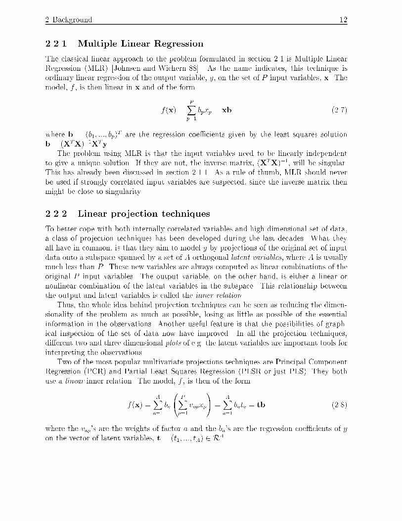
2.2.1 Multiple Linear Regression
The classical linear approach to the problem formulated in section 2.1 is Multiple Linear
Regression (MLR) [Johnsen and Wichern 88]. As the name indicates, this technique is
ordinary linear regression of the output variable, y, on the set of P input variables, x. The
model, f , is then linear in x and of the form
f(x) =PXp=1
bpxp = xb (2.7)
where b = (b1; :::; bp)T are the regression coe�cients given by the least squares solution
b = (XTX)�1XTy.
The problem using MLR is that the input variables need to be linearly independent
to give a unique solution. If they are not, the inverse matrix, (XTX)�1, will be singular.
This has already been discussed in section 2.1.1. As a rule of thumb, MLR should never
be used if strongly correlated input variables are suspected, since the inverse matrix then
might be close to singularity.
2.2.2 Linear projection techniques
To better cope with both internally correlated variables and high dimensional set of data,
a class of projection techniques has been developed during the last decades. What they
all have in common, is that they aim to model y by projections of the original set of input
data onto a subspace spanned by a set of A orthogonal latent variables, where A is usually
much less than P . These new variables are always computed as linear combinations of the
original P input variables. The output variable, on the other hand, is either a linear or
nonlinear combination of the latent variables in the subspace. This relationship between
the output and latent variables is called the inner relation.
Thus, the whole idea behind projection techniques can be seen as reducing the dimen-
sionality of the problem as much as possible, losing as little as possible of the essential
information in the observations. Another useful feature is that the possibilities of graph-
ical inspection of the set of data now have improved. In all the projection techniques,
di�erent two and three dimensional plots of e.g. the latent variables are important tools for
interpreting the observations.
Two of the most popular multivariate projections techniques are Principal Component
Regression (PCR) and Partial Least Squares Regression (PLSR or just PLS). They both
use a linear inner relation. The model, f , is then of the form
f(x) =AXa=1
ba
0@ PXp=1
vapxp
1A =
AXa=1
bata = tb (2.8)
where the vap's are the weights of factor a and the ba's are the regression coe�cients of y
on the vector of latent variables, t = (t1; :::; tA) 2 RA.

2 Background 13
PLS and PCR di�er in how the parameters vap are found, as will be explained in more
detail below. Note �rst that in neither PLS nor PCR the parameters are estimated by
�tting equation 2.8 as well as possible, as this would only lead to ordinary MLR. Instead,
quite di�erent algorithms are applied.
Principal Component Regression
In PCR, principal component analysis (PCA) [Wold et al. 87] is used to select the latent
variables. The �rst principal component, t1, is de�ned as the projection of X onto the
normalized eigenvector, w1, corresponding to the largest eigenvalue of XTX. In other
words, t1 = Xw1, where w1, the loading weight vector, can be seen as the direction
spanning most of the variability in X.
The other principal components, tp; p = 2; :::; P , are de�ned in the same way, as suc-
cessive projections of X onto the other normalized eigenvectors, wp; p = 2; :::; P , under the
constraint that the principal components are all orthogonal. These eigenvectors correspond
to the respective eigenvalues of XTX in descending order, and they will be orthogonal as
well.
Instead of computing all the eigenvalues simultaneously by e.g. singular value decompo-
sition of X, they are often computed successively in descending order, because one is only
interested in a few of them. This can be done using e.g. the NIPALS algorithm [Wold 66]:
1. Initialization: X0 = X (assumed to be scaled and centered)
2. for factor a = 1; 2; :::A compute loading vector wa and score vector ta as:
(a) Initial estimate: ta =<column in Xa�1 with highest sum of squares>
(b) repeat until <eigenvalue estimate convergence>
i. Improve estimate: wa =�tTa ta
��1XT
a�1ta
ii. Scaling: wa = wa
�wTawa
�1=2iii. Improve estimate: ta = Xa�1wa
iv. Eigenvalue estimate: tTa ta
(c) Subtract the e�ect of this factor: Xa = Xa�1 � tawTa
Since there are P eigenvalues of XTX there will be P principal components. However,
only the �rst A components are interesting since they will contain all the signi�cant vari-
ability in X. They are ordered in the matrix T = (t1; :::; tA), which can be thought of as
the input matrix X in compressed form. In PCR, the latent variables are nothing more
than these A principal components, where A is usually selected by cross-validation or test
set validation.
In the �nal step in PCR, the output variable, y, is regressed on the latent variables
using ordinary MLR, giving the regression coe�cients ba; a = 1; 2; :::; A in the general
equation 2.8. For each a, the weights, vap; p = 1; 2; :::; P , in the same equation are equal to
the elements in the loading weight vector, wa.

2 Background 14
PCR can be characterized as an unsupervised method, since the latent variables are
not found using information about the output variable, y. Instead, PCR is a variance
maximizing method, because only those latent variables which contribute the most to the
variability in X are considered.
Partial Least Squares Regression
Contrary to PCR, PLS [Wold et al. 84, Geladi and Kowalski 86, Lorber et al. 87, Höskuldsson 88]
is a supervised method, where the in�uence of y is incorporated when the latent variables
are found. PLS can also be seen as a covariance maximizing method, since it maximizes
the covariance between Xa�1wa and y under the same constraint as in PCR, wTawa = 1.
In other words, the latent component, ta, is found by projecting Xa�1 onto the direction
wa, which now is a cross between the direction with highest correlation between the input
variables and output variable (MLR approach) and the direction with largest variation in
the input variables (PCR approach) [Stone and Brooks 90].
As with the NIPALS algorithm in PCA, the latent variables are computed successively
in the PLS algorithm. Since PLS will be part of the new algorithms proposed in this thesis,
the orthogonalized form of the algorithm is given below.
1. Initialization: X0 = X and y0 = y (both assumed to be scaled and centered)
2. for factor a = 1; 2; :::Amax compute loadings wa, pa and qa and score ta as:
(a) Loading weights: wa = XTa�1ya�1
(b) Scaling: wa = wa
�wTawa
�1=2(c) Scores: ta = Xa�1wa
(d) Loadings: pa =�tTa ta
��1XT
a�1ta
(e) Output loading: qa =�tTa ta
��1yTa�1ta
(f) Subtract the e�ect of this factor: Xa = Xa�1 � tapTa and ya = ya�1 � taqa
3. Determine A, 1 � A � Amax, the number of factors to retain.
In this algorithm the score vectors, ta, and loading weight vectors, wa, are orthogonal,
whereas the extra loading vectors, pa, are generally not. A nonorthogonal form of the PLS
algorithm exists as well, where no extra loadings are needed, but resulting in nonorthogonal
latent variables or scores. Note that for neither of the two forms there is a straight-forward
relationship, for each a, between the weights vap; p = 1; 2; :::; P in the general equation 2.8
and the elements in the loading weight vector, wa. Instead the relationship is complex,
and also includes the elements in the other loading vector, pa. For the orthogonalized
algorithm it is given iteratively by v1 = w1 and va = (I �Pa�1
i=1 vipTi )wa; a = 2; :::; A,
where va = (va1; :::; vaP )T . The regression coe�cients, ba, are equal to the output loadings,
qa; 8a.
2 Background 15
The PLS algorithm shares two more common features with the PCR approach. The
number of latent variables are selected by cross-validation or test set validation, and in
the limit A = P , the PLS (and PCR) solution equals the MLR solution, i.e. equation 2.8
reduces to 2.7.
A modi�ed version of the orthogonalized algorithm, known as the PLS2 algorithm, has
been developed for the case when there is more than one output variable, but this is beyond
the scope of this thesis. For a more comprehensive description of multivariate projection
techniques see the textbook by [Martens and Næs 91].
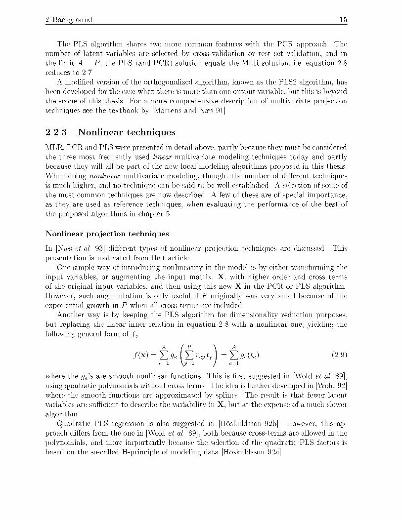
2.2.3 Nonlinear techniques
MLR, PCR and PLS were presented in detail above, partly because they must be considered
the three most frequently used linear multivariate modeling techniques today and partly
because they will all be part of the new local modeling algorithms proposed in this thesis.
When doing nonlinear multivariate modeling, though, the number of di�erent techniques
is much higher, and no technique can be said to be well established. A selection of some of
the most common techniques are now described. A few of these are of special importance,
as they are used as reference techniques, when evaluating the performance of the best of
the proposed algorithms in chapter 5.
Nonlinear projection techniques
In [Næs et al. 93] di�erent types of nonlinear projection techniques are discussed. This
presentation is motivated from that article.
One simple way of introducing nonlinearity in the model is by either transforming the
input variables, or augmenting the input matrix, X, with higher order and cross terms
of the original input variables, and then using this new X in the PCR or PLS algorithm.
However, such augmentation is only useful if P originally was very small because of the
exponential growth in P when all cross terms are included.
Another way is by keeping the PLS algorithm for dimensionality reduction purposes,
but replacing the linear inner relation in equation 2.8 with a nonlinear one, yielding the
following general form of f ,
f(x) =AXa=1
ga
0@ PXp=1
vapxp
1A =
AXa=1
ga(ta) (2.9)
where the ga's are smooth nonlinear functions. This is �rst suggested in [Wold et al. 89],
using quadratic polynomials without cross terms. The idea is further developed in [Wold 92]
where the smooth functions are approximated by splines. The result is that fewer latent
variables are su�cient to describe the variability in X, but at the expense of a much slower
algorithm.
Quadratic PLS regression is also suggested in [Höskuldsson 92b]. However, this ap-
proach di�ers from the one in [Wold et al. 89], both because cross-terms are allowed in the
polynomials, and more importantly because the selection of the quadratic PLS factors is
based on the so-called H-principle of modeling data [Höskuldsson 92a].

2 Background 16
Another technique, which is essentially based on the same model as in equation 2.9, is
Projection Pursuit Regression (PPR) [Friedman and Stuetzle 81]. In this technique, the
ga's are totally general functions except that they are smooth. As in the PLS algorithm,
one factor or latent variable, with weights vap; p = 1; 2; :::; P and function ga, is computed at
a time. The e�ect of this factor is subtracted from ya�1, and the same procedure is applied
to the residuals, ya. However, contrary to the PLS algorithm, there are no orthogonal
restrictions in the estimation of the vap's in the iterative procedure. A drawback with PPR
is that the predictor f can not be written in closed form because the ga's are only smooth
�ts to the samples in Dtrain, usually determined using moving averages. Prediction of y for
new samples must therefore be made by interpolations between the training samples. For
further discussion of projection pursuit in general, and PPR in particular see [Huber 85].
A technique called nonlinear PLS is proposed in [Frank 90]. This approach is also
essentially based on the same model as in equation 2.9, with the ga's being determined
by a smoothing procedure, as in PPR. However, the va's are estimated under exactly the
same strong restriction of covariance maximization as in PLS, which makes this technique
a kind of hybrid of PPR and PLS. The same drawback as in PPR, regarding prediction of
y for new samples, is present in this approach.
Locally Weighted Regression
In [Næs et al. 90] a technique is suggested which is a generalization of the PCR algorithm,
replacing the last MLR step with a locally weighted multiple linear regression (LWR),
thereby the name. To be more speci�c, �rst the original input hyperspace is projected
onto a lower dimensional hyperspace spanned by the latent variables ta; a = 1; 2; :::A, using
a standard PCA of X. A new input sample, xi 2 RP , will then correspond to a sample,
ti 2 RA, in the latent hyperspace. The K nearest neighboring projected samples among the
Ntrain samples in the training set are then selected, based on their Mahalanobis distance
(see appendix B.3) to ti. These samples are given a weight between 0 and 1, using a
cubic weight function, again depending on their relative distance to ti. At last, a MLR
is performed based on the K weighted samples and the corresponding K output samples.
The result is a local prediction model, f i, of essentially the same form as equation 2.8,
which is now used to predict yi. A new such local model must be computed for each single
prediction, since another input sample, xj, will lead to di�erent weighted neighboring
samples and thus a di�erent local regression model. The optimal number of neighboring
samples, K, and principal components, A, can both be determined using cross-validation
or test set validation.
LWR is a locally linear, but globally nonlinear projection technique. The drawback is
again that the predictor, f , can not be written in closed form because the prediction of y
for new samples must include the presence of the training samples in Dtrain.
In [Næs and Isaksson 92] some modi�cations to LWR are suggested, including a new
distance measure and a uniform weight function.

2 Background 17
Hidden layer
Output layer
Inputlayer
Y
ba
ap
X pX X1
g
h
P
a
v
Figure 2.2: Arti�cial neural network with one hidden layer and one output node.
Arti�cial Neural Networks
The �eld of Arti�cial Neural Networks (ANN) covers many di�erent network algorithms,
and its use has exploded in the last decade. For a good survey and other references
see the textbook by [Hertz et al. 91]. ANN has shown a lot of potential in modeling
arbitrary nonlinear relationships. The terminology of ANN is somewhat di�erent from
other techniques. These new terms will be introduced by pointing to the illustration in
�gure 2.2.
Two of the most common types of networks are Multilayered Perceptron Networks
(MLP) [McClelland et al. 86] and Radial Basis Function Networks (RBFN) [Moody and Darken 88,
Stokbro et al. 90]. Both are feed-forward networks, where the information (i.e. samples)
from the input layer is passed through intermediate variables (hidden layers) to the output
layer. These intermediate variables can be thought of as projections or transformations
of the original input variables. In the �gure there is only one hidden layer. Each layer
consists of a number of nodes. This number equals P in the input layer and is one in the
output layer. In the hidden layer(s) there are no restrictions on the number of nodes, A.
Each node, except those in the input layer, is usually connected with all the nodes in the

2 Background 18
previous layer. These connection lines will all have di�erent weights, denoted vap and ba in
the �gure. In each node, the weighted information from the previous layer is transformed
by transfer functions, denoted ha and g, before being passed to the next layer. The trans-
formation is very di�erent in MLP and RBFN. The output from the network will have the
general form
f(x) = g
0@ AXa=1
baha
0@ PXp=1
vapxp
1A1A (2.10)
A bias term can also be added to each node in the hidden and output layer before the
transformation, but this is not illustrated in the �gure nor in equation 2.10.
In MLP the transfer functions are typically sigmoid shaped e.g. ha(z) = tanh(z) or
ha(z) = 1=(1 + exp(�z)). The most common learning algorithm is error back propaga-
tion (BP) [Rumelhart et al. 86], which is a gradient descent algorithm �nding the optimal
weights by usually minimizing the sum of squared estimation sample errors, or a variation
thereon.
In RBFN there is always only one hidden layer, all the vap's are equal to 1 and g is
the identity transformation. Thus, the input to the transfer functions ha is no longer a
weighted sum. The model f is then reduced to the form
f(x) =AXa=1
baha(r) (2.11)
where the ha's are scalar radial basis functions centered around the extra parameter vec-
tors �a and r = kx � �akM. Examples of basis functions are the logarithmic function
ha(r) = log(r2 + c2), where c is a constant, and the Gaussian function ha(r) = exp(�1
2r2).
Again, a gradient descent algorithm is usually applied to iteratively estimate the network
parameters. A good overview of RBFN is given in [Carlin 91].
Observe that the di�erent learning algorithms in ANN are just ways of �nding the
optimal parameters from the training samples, which are presented to the network in
random order. Generally, this is a slow procedure compared to other nonlinear techniques.
A comparison between MLP and RBFN has shown that MLP is slower, requires more
layers, but less samples and hidden nodes than RBFN to obtain the same level of accuracy
[Moody and Darken 89]. In addition, RBFN does not work too well when data are high
dimensional because of the necessity of a distance measure in the radial basis functions,
ha.

2 Background 19
X1
X2
X3
X4
X5
X6
X7
X8
g(X1,X2)
g(X3,X4,X5)
g(X6)
Submodel 1
Submodel 2
Submodel 3
+ Y
Figure 2.3: The MARS and ASMOD model structure.
Adaptive spline techniques
Multivariate Adaptive Regression Splines (MARS) [Friedman 88] and Adaptive Spline
Modeling of Observation Data (ASMOD) [Kavli 92] are two techniques that represent f
by the decomposition exempli�ed in �gure 2.3. The general form of the model is given by
f(x) =X
gi(xi) +X
gij(xi; xj) +X
gijk(xi; xj; xk) + ::: (2.12)
In both algorithms, a subset of the possible submodels, g, are selected during the
training process. Both apply splines in the function representation of the submodels,
although MARS employs natural splines as opposed to B-splines which are used in ASMOD.
Generally, splines have great abilities of approximating multivariate functions by joining
polynomial segments (basis functions) to form continuous and smooth functions. For more
comprehensive presentations of splines see [Farin 88, Wahba 90].
MARS is a two-step algorithm. The �rst step is a forward partition step decomposing
the input space into a number of overlapping submodels. The second is a backward pruning
step deleting those submodels which contribute the least in the �t based on the GCV
criterion (see equation 2.6).
In ASMOD both of these steps are combined in one iterative model re�nement proce-
dure. In each step in the iteration either a new one-dimensional submodel is added, two
submodels are replaced by one higher dimensional submodel, or a new knot is inserted in
the B-spline of any of the submodels, depending on which of the three ways reduced the
estimation error the most. The re�nement is terminated when the prediction error is at a
minimum.

2 Background 20
This way of decomposing will include only the submodels for input variables that are
necessary in the prediction of y. With strongly correlated variables only limited improve-
ment of the predictions can be expected when more than a few of the variables are added to
the model. Thus, the adaptive spline techniques aim at keeping the number of submodels
to a minimum. At the same time, they can be seen as modeling high dimensional data by
a sum of lower dimensional submodels, as the dimensionality of the submodels are kept as
low as possible.

3
Local modeling
An interesting approach to nonlinear empirical modeling is local modeling. In this chapter
the modeling philosophy behind this approach is presented and discussed. The presentation
serves as an introduction to the proposed local modeling algorithms in chapter 4. The
model, f , is then of the general form
f(x) =MXm=1
wm(x)fm(x) (3.1)
where fm is the local model, wm the corresponding weight function, and M the total
number of local models.
Local modeling is characterized by the decomposition of the input hyperspace into
smaller local hyperspaces with equal dimension. A simple local model is found in each of
these hyperspaces. Such a model will only describe local variations, since it will only be
based on training samples within the local hyperspace. All these local models are then
interpolated by the use of local weight functions, yielding the total model f . This model
should have better predictive ability than a simple global model, otherwise there is no need
for a local approach.
The major problems that are speci�c to local modeling are:
� How to divide the input hyperspace?
� How to decide the optimal number of local models, M?
� How to interpolate between the local models?
� How to represent the local models, using which algorithm?
These problems will be addressed in this chapter. A more statistical discussion of mul-
tivariate calibration when data are split into subsets is found in [Næs 91]. Two approaches
to local modeling, which are related to the work of this thesis and have proved to be in-
spiring, are an algorithm using fuzzy clustering by [Næs and Isaksson 91] and the local
search algorithm (LSA) in [Johansen and Foss 93]. Details about them will be presented
in the subsequent sections in this chapter as examples of di�erent ways of dealing with the
problems mentioned above.
21
3 Local modeling 22
3.1 Division of input space
The most fundamental problem in local modeling is how to divide the input hyperspace
in a parsimonious way such that the number of local models is kept at a minimum, but
is still su�cient to adequately model the system, in the sense described in section 2.1.2.
This problem is closely linked to that of how many local models the hyperspace should be
divided into. As one has very little a priori knowledge about the system, the exact number
and precise position of these models are not known in advance.
One possibility is to construct a grid in the hyperspace and then include local models
around those grid points, where there are enough samples. However, this static approach
is both time consuming and impractical in high dimensional spaces. With a uniform (equal
spacing) and homogeneous distribution of grid points in every dimension, the result is an
exponential growth in the number of grid points and local models (see section 2.1.1). Thus,
even with relatively few grid points in each dimension, the number of local models will be
very large. Another drawback is that all the local models will be valid in equal sized local
hyperspaces. Often some of them can easily be replaced by a larger one, without reducing
the overall e�ect.
A more dynamic approach is to apply a clustering algorithm. Such an algorithm seeks
to cluster the samples together in M disjunct groups, by minimizing the total spatial
(Euclidian or Mahalanobis) distance between all the samples within a group. The number
of groups, M , does not always have to be known in advance, although it is often required.
Many di�erent algorithms are available, both hierarchical, nonhierarchical and a hybrid of
those. For a good survey see [Gnanadesikan et al. 89].
One drawback using traditional clustering algorithms is that they only consider close-
ness in space when samples are assigned to di�erent groups. This might be desirable in
classi�cation problems, but since the purpose of this thesis is prediction, and not classi�-
cation, that aspect should also be re�ected in the decomposition algorithm.
One way of doing this is suggested in [Næs and Isaksson 91]. There, a division of the
input space is proposed based on a fuzzy clustering algorithm [Bezdec et al. 81], with M
�xed. However, the distance measure is now a weighted combination of the Mahalanobis
distance (from traditional clustering) and the squared residuals from local �tting of the
samples. After the convergence of the clustering algorithm, each sample is allocated to
the group for which it has the largest so-called membership value. This fuzzy clustering
algorithm is part of an approach to local modeling which is based on many of the same
principles as in LWR. First, the input hyperspace is projected using a standard PCA.
Then, after the clustering algorithm is applied to all the projected training samples, a
separate linear regression is performed within each group, resulting in M locally linear
PCR models. However, these models are not interpolated, so f in equation 3.1 will not
be smooth. Instead, new samples are simply allocated to the closest class by an ordinary
Mahalanobis distance method in traditional discriminant analysis. The optimal number of
local models is found by cross-validation or test set validation.

3 Local modeling 23
X1
X2
Model 1 Model 3
x
xx
x x
x x
x x
xx
x
x
x
x
x
x
xx x
xxx
x
x xx
x x
x
x
x
x
x
x
x
x
x
X1,maxX1,min
X2,min
X2,max
Model 2
Figure 3.1: Splitting of the input space into rectangular boxes in the LSA algorithm.
Another approach is an iterative decomposition into smaller and smaller hyperspaces. A
prime example is applied in the LSA algorithm [Johansen and Foss 93], which divides the
input space into hyperrectangles (see �gure 3.1 for an illustration). In each iteration one of
the hyperrectangles is split into two smaller ones. Which hyperrectangle should be split and
how is decided by testing several alternatives and choosing the one that gives the largest
decrease in a validation criterion. The LSA algorithm also involves local linear models and
smooth interpolation between the local models by the use of Gaussian functions.
The approach was originally developed for NARMAX models [Johansen and Foss 92a,
Johansen and Foss 92b], but has been extended to general nonlinear dynamic and static
models. The algorithm involves no projection of the input variables as a result of being
developed in a system identi�cation context. It is therefore best suited for lower dimensional
problems, and all the present experience is on that kind of problems. However, as suggested
in [Johansen and Foss 93], it can easily be expanded to high dimensional problems by �rst
carrying out a principal component projection as is done in [Næs and Isaksson 91].
Other examples of iterative decompositions can be found in the MARS [Friedman 88]
and CART [Breiman et al. 84] algorithms.
The clustering algorithms and the two approaches outlined above are all using so-called
`hard' splits of data. This means that each sample only belongs to one local hyperspace
and thus only contributes to one local model. Such a split is known to increase the variance
[Jordan and Jacobs 94]. The alternative is `soft' splits of data, which allow samples to lie
simultaneously in multiple hyperspaces.

3 Local modeling 24
3.2 Validation and termination of modeling algorithm
No matter how one divides the input space, there will always be need for validating an
actual splitting because one wants to determine the optimal one. Optimal, in the sense
that this splitting gives the largest improvement in prediction ability, compared to other
splittings of the same input space and with di�erent numbers of local models, M .
If M is �xed in the decomposition algorithm, the common approach is either cross-
validation or test set validation.
However, in an iterative decomposition algorithm the validation must be done after
each iteration since each step will produce a new splitting of the data and increase the
number of local models by one. Another important aspect in an iterative algorithm is to
determine when to end the re�nement of the model, f .
These two tasks can be combined using either test set validation, cross-validation, or
other types of validation (see section 2.1.4) and stopping the iteration when one of the
estimators has reached a minimum value. An example is the application of the FPE and
GCV criterion in the LSA algorithm [Johansen and Foss 93].
An alternative is to have a separate validation criterion and a stop criterion, which is
based on the evolution of the estimation error (MSEE). One such stop criterion is to end
the re�nement when the MSEE is levelling out, i.e. the di�erence between the MSEE in
the last and second-to-last step is lower than a prede�ned value. However, this is only
recommended when the danger of over�tting is reduced due to relatively little noise in the
data and when Ntrain is large.
Another approach is to stop iterating when the MSEE becomes smaller than a prespec-
i�ed limit. This limit should be set slightly higher than the anticipated noise level, in order
to avoid modeling random noise. This approach is only advisable when a good estimate of
the noise level is available.
Both these somewhat ad hoc approaches are motivated by �gure 3.2 which shows a
typical behavior of the prediction error (MSEP) and MSEE, as the complexity of f , i.e.
number of local models, increases. The �gure also illustrates the e�ect of over�tting when
random noise is modelled.
The very best approach when validating and terminating an iterative algorithm is to
have three, all representative and independent, data sets:
� A training set, used to compute the parameters in f .
� A stop set, used to determine when to stop re�ning f in the training step.
� A test set, used to validate the �nal prediction ability of f .
If the data sets are representative this will be a completely unbiased estimate. Unfor-
tunately, this approach is usually not feasible since it requires too much data.

3 Local modeling 25
Model complexity
Error
Prediction error (MSEP)
Estimation error (MSEE)
Figure 3.2: General evolution of the estimation error (MSEE), and the prediction error
(MSEP), as a function of increasing model complexity.
3.3 Weighting and interpolation
All the local models will have a limited range of validity. One therefore needs to determine
how to interpolate them to yield a complete global model, f . Having no interpolation at
all will lead to a rough or even discontinuous f , which is undesirable.
One way is to assign a normalized and smooth weight or interpolation function to each
local model. Such a function is often of the form
wm(x) =�m(x)PMj=1 �j(x)
(3.2)
where �m is a scalar local validity function [Johansen and Foss 92a], which should indicate
the validity or relevance of the local model as a function of the position of x in input space.
Furthermore, �m should be nonnegative, smooth, and have the property of being close to
0 if x is far from the center of a local model. The use of smooth validity functions, along
with smooth local models, fm, ensures that f will be smooth as well.
Ideally, the sum of the validity functions at any position, x, in the input space should
be equal to unity. This can be achieved in practice by normalizing the �m's. One is then
ensured that the total weight given to x from all the local models is always unity, becausePMm=1 wm =
PMm=1 �m=
PMj=1 �j = 1; 8x. However, there is also a danger using this way of
weighting, as extrapolation to regions in input space outside the operating regime of the
system is now very easy. This is not always advantageous.

3 Local modeling 26
-1-0.5
00.5
1
-1
-0.5
0
0.5
10
0.2
0.4
0.6
0.8
1
X1X2
Valid
ity, rh
o
Local Gaussian validity function
Figure 3.3: A two dimensional unnormalized Gaussian function.
Since the validity function is centered around a local model, one needs to de�ne the
center, �m. Usually, �m, is de�ned to be either the mean vector of all the training samples
in class m (center of `mass'), or the center of the local hyperspace itself if the space
has properly de�ned boundaries (geographical center). One example of the latter is the
hyperrectangular region in the LSA algorithm, where �m is the center of the box.
Probably the most used validity function is the unnormalized Gaussian function. The
general form of this multivariate function is
� = exp(�1
2(x� �)��1(x� �)T ) (3.3)
where � is the center of the local validity function and � is a smoothing matrix which will
de�ne the overlap between the di�erent local validity functions. In one dimension, � can
be thought of as the squared standard deviation or the width of the Gaussian function. A
two dimensional example is given in �gure 3.3.
3 Local modeling 27
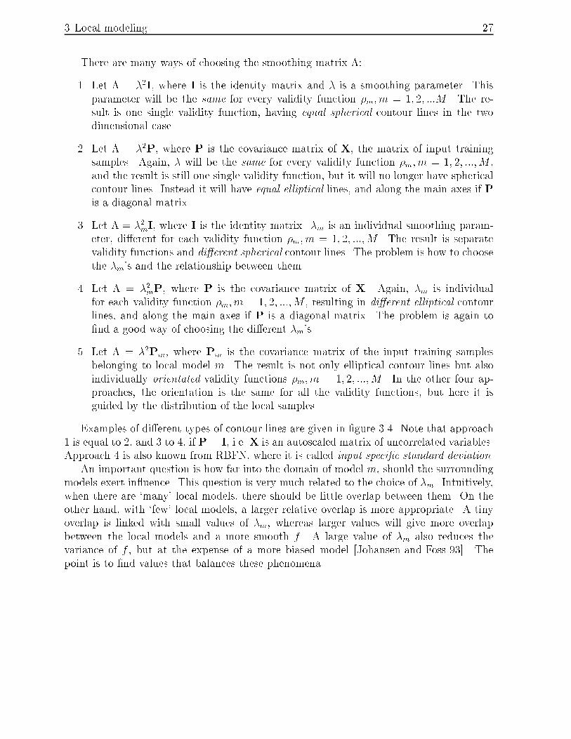
There are many ways of choosing the smoothing matrix �:
1. Let � = �2I, where I is the identity matrix and � is a smoothing parameter. This
parameter will be the same for every validity function �m; m = 1; 2; :::M . The re-
sult is one single validity function, having equal spherical contour lines in the two
dimensional case.
2. Let � = �2P, where P is the covariance matrix of X, the matrix of input training
samples. Again, � will be the same for every validity function �m; m = 1; 2; :::;M ,
and the result is still one single validity function, but it will no longer have spherical
contour lines. Instead it will have equal elliptical lines, and along the main axes if P
is a diagonal matrix.
3. Let � = �2mI, where I is the identity matrix. �m is an individual smoothing param-
eter, di�erent for each validity function �m; m = 1; 2; :::;M . The result is separate
validity functions and di�erent spherical contour lines. The problem is how to choose
the �m's and the relationship between them.
4. Let � = �2mP, where P is the covariance matrix of X. Again, �m is individual
for each validity function �m; m = 1; 2; :::;M , resulting in di�erent elliptical contour
lines, and along the main axes if P is a diagonal matrix. The problem is again to
�nd a good way of choosing the di�erent �m's.
5. Let � = �2Pm, where Pm is the covariance matrix of the input training samples
belonging to local model m. The result is not only elliptical contour lines but also
individually orientated validity functions �m; m = 1; 2; :::;M . In the other four ap-
proaches, the orientation is the same for all the validity functions, but here it is
guided by the distribution of the local samples.
Examples of di�erent types of contour lines are given in �gure 3.4. Note that approach
1 is equal to 2, and 3 to 4, if P = I, i.e. X is an autoscaled matrix of uncorrelated variables.
Approach 4 is also known from RBFN, where it is called input speci�c standard deviation.
An important question is how far into the domain of model m, should the surrounding
models exert in�uence. This question is very much related to the choice of �m. Intuitively,
when there are `many' local models, there should be little overlap between them. On the
other hand, with `few' local models, a larger relative overlap is more appropriate. A tiny
overlap is linked with small values of �m, whereas larger values will give more overlap
between the local models and a more smooth f . A large value of �m also reduces the
variance of f , but at the expense of a more biased model [Johansen and Foss 93]. The
point is to �nd values that balances these phenomena.

3 Local modeling 28
-1 -0.5 0 0.5 1-1
-0.5
0
0.5
1
X1
X2
Gaussian contour lines, lambda=1
-1 -0.5 0 0.5 1-1
-0.5
0
0.5
1
X1
X2
Gaussian contour lines, lambda=1
-1 -0.5 0 0.5 1-1
-0.5
0
0.5
1
X1
X2
Gaussian contour lines, lambda=1/2
-1 -0.5 0 0.5 1-1
-0.5
0
0.5
1
X1
X2
Gaussian contour lines, lambda=1/2
Figure 3.4: Gaussian contour lines for di�erent choices of �. (a) Identity matrix, � = 1.
(b) Diagonal matrix, � = 1. (c) Identity matrix, � = 12. (d) Diagonal matrix, � = 1
2.

3 Local modeling 29
Another aspect is that since distance metrics are involved, all weighting and interpolat-
ing should take place in a projected low dimensional space and not in the original, possibly
high dimensional hyperspace. If PCA is utilized as the projection technique, reducing X to
the latent matrix T, the covariance matrix of T will have the favorable property of being
diagonal in approaches 2 and 4. The validity functions (and weight functions) will then be
functions of the latent variables, i.e. �m = �m(t) (and wm = wm(t)), and not of the original
input variables.
Typical other choices of validity function are linear, quadratic or cubic splines and
other well-known kernel-functions [Hastie and Tibshirani 90]. A more odd choice is to
use indicator functions. This is equivalent to giving no weight to all but one of the lo-
cal models, which will have unit weight. An example is the local modeling approach of
[Næs and Isaksson 91]. As already mentioned, the result is no longer a smooth f .
3.4 Local type of model and optimization
One of the advantages with local modeling is that the structure of the local models, fm,
does not need to be very complex. Usually simple linear models are su�cient. The model,
f , is still a good nonlinear predictor. However, the complexity is not in the local models
themselves, but in the interpolation between them.
In this thesis only local models with linear model structure in the input variables x are
used. The next problem is, as it was in global modeling, which mathematical algorithm to
use for estimating the local parameter values. Since high dimensional input samples are
assumed, focus will be on projection techniques such as PCA. Two techniques are then
evident. Either MLR of y on the latent input variables, t, or PLS modeling of y on the
original input variables, x.
The �rst approach is used in the algorithm proposed in [Næs and Isaksson 91], and will
produce local PCR models. Each local MLR takes place in the same latent input space
as the weighting does. In the second approach one applies the original input variables in
each local PLS. The number of latent variables will then possibly be di�erent for each local
model. However, all weighting is still done in the same latent space, as found by the PCA
algorithm.
An important question is whether the parameters in the local models should be opti-
mized locally or globally. In a local optimization, each local model is optimized separately
and then weighted, yielding the global model, f . A global optimization will optimize all
the local parameters simultaneously, and should provide a better approximation of y on
the training samples. On the other hand, when f is presented with new samples the per-
formance can be worse as local optimized models are often more representative of the local
behavior of the system than globally optimized ones [Murray-Smith 94].

3 Local modeling 30
Using MLR as the local modeling technique, both local and global optimization can
be done with a standard weighted least squares algorithm. However, if PLS is applied, a
global optimization would be very time consuming since the global optimal combination
of di�erent numbers of local latent variables, from di�erent local PLS algorithms, must be
obtained by e.g. cross-validation. This is a formidable task even for a small number of local
models. In that case only local optimization is feasible. What is still a problem, though,
is that a PLS algorithm with individual weighting of the input samples, which would have
been desirable, does not exist to the best of my knowledge.
Although the focus in this thesis is on local linear models, that does not completely rule
out selecting nonlinear local models and a nonlinear algorithm. But, usually very little is
gained in prediction ability with such an approach. At least when compared to the much
increased computational cost, which is unavoidable once the step from linear to nonlinear
local models is taken.

4
Proposed algorithms
In this chapter three new algorithms for local modeling are proposed. The �rst, a local
search algorithm, is the main algorithm of this thesis. Four di�erent versions of this
algorithm are presented in detail, all of which were implemented and tested. The other two,
a global search algorithm and an extended local search algorithm, were not implemented
and are just brie�y described. All the algorithms give rise to models of the general form
given in equation 3.1.
Before starting to develop the algorithms, a few important choices regarding the struc-
ture of the algorithm and solution, f , have to be made. These choices are taken on the
basis of the discussion in chapter 3.
� The algorithms are based on an iterative splitting of the input space into local regions,
implying a gradual re�nement of f .
� The local regions have a �exible shape, and are not restricted to e.g. hyperrectangular
boxes. With more complex region boundaries it is anticipated that a smaller number
of local models is needed, but at the expense of more parameters for describing the
regions.
� `Hard' splits of data are used, with the local regions being disjunct. Each training
sample will then contribute to one and only one local model.
� The interpolation between the local models is done with smooth, normalized weight
functions and Gaussian validity functions. The input set of data is typically projected
onto a lower dimensional subspace based on its �rst few principal components. Local
weighting is then carried out in this subspace.
� Linear functions are used in the local models, with PLS as the local modeling tech-
nique.
31

4 Proposed algorithms 32
The total model, f , then has the speci�c form found by substituting equation 3.2
(normalized weight function) and 2.8 (PLS model) into equation 3.1 yielding
f(x) =MXm=1
�m(t)PMj=1 �j(t)
0@AmXa=1
bma
0@ PXp=1
vmapxp
1A+ bm0
1A (4.1)
where Am is the number of latent variables in local PLS model m and bm0 is a constant
term.
As the latent variables are only linear combinations of the input variables, equation 4.1
can be reduced to
f(x) =MXm=1
�m(t)PMj=1 �j(t)
0@ PXp=1
bmpxp + bm0
1A =
MXm=1
wm(t)fm(x) (4.2)
without loss of generality. This is the form of f used in the discussion.
It can be shown mathematically that f can approximate any so-called measurable func-
tion arbitrary well. The details are omitted here, but the reasoning is that any measurable
function can be approximated arbitrary well by a piecewise constant function. Thus, in
equation 4.2, setting bmp = 0; 8m; p gives piecewise constant functions, and anything that
can be approximated by piecewise constant functions can also be approximated by f , and
anything that can be approximated by f can also be approximated by piecewise constant
functions. The only condition is that the validity function �m must be allowed to be the
indicator function, �R, as well as e.g. the Gaussian. The complete proof is given in e.g.
[Folland 84].
�R(t) =
(1 t 2 R
0 t 62 R
(4.3)
So, theoretically the model structure in equation 4.2 should be able to handle any type
of empirical modeling problem, at least when the number of samples, N , and the number
of local models, M , go towards 1. Practically though, N and M are of course bounded,
which limits the prediction ability, as does the presence of noise in the observations.

4 Proposed algorithms 33
1. Preprocessing of the data set, D.
2. Initialization.
� De�ne validity function �1.
� Compute initial global linear model, f (1) = f1.
� The number of local models, M = 1.
3. while <consistent decrease in validation criterion J> do
� Find the local region where f (M) is modeling the worst.
� Allocate training samples to the M + 1 di�erent local regions.
� De�ne new validity functions �m.
� Compute new local linear models, fm, in these regions.
� Interpolate, f (M+1) =P
mwmfm.
� Validate f (M+1) using validation criterion J .
� Increment, M =M + 1.
4. Determine the optimal model, f .
Figure 4.1: General Algorithm 1.
4.1 General Algorithm 1
The approach can be described as an iterative structure identi�cation algorithm, based
on error analysis of samples. The general Algorithm 1 consists of the steps given in
�gure 4.1.
A total of four di�erent versions of this algorithm are proposed, but only two proved
to work well. The di�erence between them is in the repeated step (3), which constitutes
the heart of the algorithm. The other steps (1, 2, 4) are essentially the same all the time.
All the four steps are now explained in detail. To make the presentation as easy to
grasp as possible, this is �rst done by describing the complete Algorithm 1a, which is
the most important, in the next section. The other three algorithms, 1b, 1c, and 1d are
then explained in section 4.3.

4 Proposed algorithms 34
4.2 Algorithm 1a
Preprocessing (step 1)
This step �rst includes removal of possible outliers from the data set, D. Since this algo-
rithm is based on error analysis of samples, abnormal observations could strongly in�uence
the results of the algorithm.
Then, D is divided into separate training (Dtrain) and test sets (Dtest), both equally well
distributed and representative of the system that is to be modelled.
The last step in the preprocessing is to select the �rst few (2�4) principal components
of the input training matrix as a subspace used for weighting between the local models.
The components are found by PCA analysis and the number of components are denoted
by Aw.
After these initial operations, there are six di�erent matrices. The training samples in
Dtrain are organized in the input matrix X and the output matrix y, both of which are
assumed to be scaled and centered. The test samples in Dtest are gathered in the input
test matrix Xtest and the output test matrix ytest. The variables in these two matrices are
assumed to be scaled and centered with the same factors as the variables in the training
matrices. In addition, the projected input training samples are assembled in the matrix T.
The last matrix is Ttest, consisting of the input test samples projected onto the weighting
subspace. The original input space formed by the input training samples are denoted by
O, and the projected input subspace by W . There is always a one-to-one correspondence
between a sample xi in O and a sample ti in W .
Initial model (step 2)
An initial local linear model, f1, based on all the samples in the training set, is computed
by the PLS algorithm. Since there is only one local model this is also the total model, f (1).
A local model validity function �1 is de�ned, having the center in origo of W , i.e. �1 = 0.
Origo is the natural choice since T has zero column mean.
Finding local region (step 3)
The whole idea behind the approach is to insert a new local model where the current model,
f(M), is predicting worst. In other words, identify the local region where the expected
deviation E[jy� �yj] is largest. This region in input space will be represented by one of the
samples in the training set Dtrain, named the splitsample and denoted xsM , where sM is the
splitsample index. The new local model is computed around that sample.

4 Proposed algorithms 35
Finding this splitsample is the purpose of this step. Di�erent ways of doing this are
proposed. But, �rst a few de�nitions that are essential for understanding the principles.
All the de�nitions below are to be associated with one input training sample, xn.
i. Single error, en(1). De�ned as the absolute error jf(M)(xn)�ynj, where f (M) is the total
model after M iterations.
ii. Mean error, en(K). De�ned as the absolute mean error jPK
k=1(f(M)(xk)�yk)=Kj of the
K nearest neighboring samples to xn, using the Mahalanobis distance with covariance
matrix of T in projected input subspace. xn is included among the K samples.
iii. Median error, en(K). De�ned as the median error of the single errors in the K nearest
neighboring samples (xn included) using the Mahalanobis distance.
iv. Consistent. A sample xn is said to have a consistent error if the signs of the single
errors of the K nearest neighboring samples all are either plus or minus.
The general term sample error, denoted by en, is from now on used when referring to
one of the error measures of type i., ii., or iii..
Of the three types, the single error is the one most sensitive to outliers, since only
information about the sample, xn, is considered. The two other types use information
from surrounding samples as well, when trying to describe the error around xn, and are
therefore less sensitive to noisy samples. In particular, the median error will be unbiased
of any outliers.
The last de�nition will put a further requirement on a possible splitsample, by de-
manding that the closest surrounding samples should all have the same error behavior. If
a sample has a consistent error, it is an indication that f (M) really is not predicting well
around that sample. The term is a heuristic to be used in combination with one of the
three types of error measure, in order to further avoid selecting an outlier.
The strategy for determining the splitsample is now described. In section 4.6 an alter-
native strategy is proposed. That, however, turned out to be worse than this one.
Strategy 1
Select the splitsample as the sample of all the Ntrain samples having the largest sample error
of type i.,ii. or iii..
This strategy performs in each iteration a global search for the splitsample among all
the training samples, computing a sample error for each of the samples.
One restriction is that a training sample can not be picked twice. The splitsample is
therefore always selected as the sample with the largest error, not previously selected. In
other words, the splitsample is picked among Ntrain+1�M training samples and not Ntrain
as stated in strategy 1.

4 Proposed algorithms 36
Figure 4.2: Local regions in input subspace, with boundaries and centers.
Allocation (step 3)
Once a new splitsample is found, a new validity function �M+1 is de�ned having the center
in the projection of this splitsample, i.e. �M+1 = tsM . There will then be a total of M + 1
di�erent validity functions with centers in M + 1 geometrical points (M splitsamples plus
origo) in W . These points de�ne M + 1 classes. The goal is to allocate all the samples in
Dtrain to one, and only one, of these classes. This is done by allocating a sample to the
class for which the validity function has the largest value, or expressed mathematically
Class m = fxn; ynj arg maxj=1;2;:::;M+1
(�j(tn)) = mg (4.4)
This classi�cation divides up the projected input space into polyhedral regions as shown
in �gure 4.2. The division is known as a Voronoi (or Dirichlet) tessellation, and is often
used in data compression [Hertz et al. 91].

4 Proposed algorithms 37
Local model computation (step 3)
Since global optimization of the parameters is di�cult when PLS is the local modeling
technique (see section 3.4), local optimization is applied. Each local PLS model is found
using the original input samples and not the projected ones.
The local training samples allocated to class m are gathered in a local input matrix Xm
and output matrix ym, with Nm being the number of local samples. Before a local model fmis computed the matrices Xm and ym must be centered as required by the PLS algorithm.
The local constant term bm0 is then equal to (ym � xmbm) = (y(ym)�P
p bmpx(xmp)).
The number of latent variables in each PLS model, Am, is determined by local cross
validation. All the local models f1; f2; :::; fM+1 must be computed in each iteration since
one never knows whether the allocation of samples to some regions is the same as in the
previous iteration. The weights w1(tn); w2(t
n); :::; wM+1(tn) (see equation 3.2) belonging
to sample xn are not used in the optimization process. Note that the validity functions,
�1; �2; :::; �M+1 are applied both in the allocation of samples and in the weighting of the
local models.
Validation (step 3)
To investigate the total model f (M+1) in each iteration, both the root mean square error of
estimation (RMSEE) and the root mean square error of prediction (RMSEP) are computed.
The iteration is stopped when no further improvement is expected i.e. when the RMSEE
might still be decreasing, but the RMSEP is consistently increasing. With consistently
increasing is meant that the RMSEP increases in two preceeding steps. Admittedly this is
a somewhat ad hoc stop criterion. The reason is to avoid an early termination because of
local minima.
Optimal model (step 4)
The optimal model, f , is de�ned to be the one where the corresponding RMSEP is at a
minimum. This RMSEP value is also used as the validation value of f . As noted earlier,
doing this is a bit questionable, since the test set Dtest will no longer be unbiased. The best
would have been to have a third set of data, independent from the other two, and validate
f on that set.
The entire Algorithm 1a is summarized in �gure 4.3. The algorithm was implemented
with all the three types of error measure and the consistent de�nition. A few assumptions
regarding the local PLS modeling had to be made. They can be found, along with some
further details about the implementation, in appendix A.

4 Proposed algorithms 38
1. Preprocessing:
(a) Removal of possible outliers from Dtrain and Dtest.
(b) Training matrices: X and y (both assumed to be scaled and cen-
tered).
(c) Test matrices: Xtest and ytest (both scaled and centered with same
factors as for the training matrices).
(d) PCA analysis: Determine Aw from X.
(e) Projected input matrices: T and Ttest.
2. Initialization:
(a) De�ne validity function: �1 = exp(� 12 (t��1)�
�1(t��1)T ) where
�1 = 0, � = �2P =, and P is the covariance matrix of T.
(b) Compute global PLS model f (1) = f1 from X and y.
(c) Number of local models, M = 1.
3. while <consistent decrease in validation criterion J> do
(a) Find splitsample: �M+1 = tsM where
sM = argmaxn=1;:::;Ntrain(6=s1;:::;sM�1)(en) and
en = e
n
(1) or en
(K) or en
(K) (and tsM is consistent).
(b) De�ne validity function: �M+1 = exp(� 12(t� �M+1)�
�1
(t� �M+1)T ).
(c) for samples n = 1; 2; :::; Ntrain do
� Allocate sample xn to Xm and yn to ym using equation 4.4.
(d) Local training matrices: X1;X2; :::;XM+1 and y1;y2; :::;yM+1
(all assumed to be centered).
(e) for region m = 1; 2; :::;M + 1 do
� Compute local PLS model fm from Xm and ym.
(f) Interpolate: f (M+1) =P
mwmfm.
(g) Validate f (M+1) using validation criterion
J = RMSEP(f (M+1)(Xtest);ytest).
(h) Increment: M =M + 1.
4. Optimal model: f = argminf�=f (1);:::;f (M�1)(RMSEP(f�(Xtest);ytest)).
Figure 4.3: Algorithm 1a (Fixed validity functions).

4 Proposed algorithms 39
r
Figure 4.4: The concept of radius in local modeling (Identity matrix).
4.3 Algorithm 1b, 1c, and 1d
In the approach so far, the local validity functions have been �xed (see point 2 in section 3.3)
and `hard' splits of the training samples have been used. This is rather rigid. A more �exible
approach is perhaps `soft' splits and di�erent sized validity functions, e.g. depending on
the distance between or density of such functions.
In this section three modi�ed versions of Algorithm 1a are presented. The changes
in the algorithm only involve the allocation and local computation steps. How to �nd the
splitsample and how to validate are not altered.
The distances between the centers of local validity functions are essential in all the three
modi�cations. To each local model an extra parameter named the radius, and denoted
rm, is speci�ed. This radius is de�ned to be the smallest Mahalanobis distance, with
covariance matrix of T, between the local splitsample, �m, and all the other splitsamples
(origo included), or expressed mathematically
rm = minj=1;:::;m�1;m+1;:::M
(k�j � �mkM) (4.5)
As previously noted, the local splitsample and the center of the local validity function are
the same. An illustration of this approach is given in �gure 4.4.

4 Proposed algorithms 40
Both allocation of training samples and de�nition of validity functions can be based on
this new term.
Allocate to one class, m, all the training samples within distance rm from the center of
that class, �m, and use those samples in the computation of the local model. One training
sample can then be allocated to several di�erent classes, or it does not have to be classi�ed
at all, which happens when the sample is in a region not `covered' by the radii of any of
the local classes (e.g. the shaded region in �gure 4.4). `Soft' splits are the result. The
only requirement is that a minimum number of samples have to be allocated to each class,
in order to avoid abortion of the algorithm because of too few samples in a local region.
Expanding rm accordingly will ensure that this is always the case. The same e�ect could
possibly be achieved by somehow de�ning a minimum radius, rmin, instead, but is not
considered in this thesis.
De�ne validity functions, �m, by the use of individual smoothing parameters of the
form �m = �rm, where � is a �xed parameter. This corresponds to point 4 in section 3.3.
The result is the same overlap when splitsamples are close, as when they are far from each
other.
Algorithm 1b (Variable validity functions)
This algorithm is similar to the original Algorithm 1a, as the allocation of training sam-
ples is still based on `hard' splits, by using the same procedure described by equation 4.4.
However, the local validity functions are now individually de�ned.
Once a new splitsample is found, a new local radius, rM+1, is computed. All the other
radii a�ected by the position of the new splitsample are also re-computed. New local
validity functions with new smoothing parameters are de�ned for the regions concerned.
A new classi�cation can then take place, based on the largest values of all the validity
functions, before new local linear models are computed. The entire algorithm is given in
�gure 4.5.

4 Proposed algorithms 41
1. Preprocessing:
(a) Removal of possible outliers from Dtrain and Dtest.
(b) Training matrices: X and y (both assumed to be scaled and cen-
tered).
(c) Test matrices: Xtest and ytest (both assumed to be scaled and
centered with same factors as for the training matrices).
(d) PCA analysis: Determine Aw from X.
(e) Projected input matrices: T and Ttest.
2. Initialization:
(a) De�ne validity function: �1 = exp(� 12 (t��1)�
�1(t��1)T ) where
�1 = 0, � = �21P = (�r1)
2P, r1 = maxn=1;:::;Ntrain(ktn � �1kM),
and P is the covariance matrix of T.
(b) Compute global PLS model f (1) = f1 from X and y.
(c) Number of local models, M = 1.
3. while <consistent decrease in validation criterion J> do
(a) Find splitsample: �M+1 = tsM where
sM = argmaxn=1;:::;Ntrain(6=s1;:::;sM�1)(en) and
en = e
n
(1) or en
(K) or en
(K) (and tsM is consistent).
(b) De�ne radius: rM+1 = minm=1;:::;M(k�m � �M+1kM)
(c) for radius m = 1; 2; :::;M do
� Diminish rm if k�m � �M+1kM < rm.
(d) for region m = 1; 2; :::;M + 1 do
� De�ne validity function: �m = exp(� 12(t��m)�
�1(t��m)T )
where � = (�rm)2P.
(e) for sample n = 1; 2; :::; Ntrain do
� Allocate sample xn to Xm and yn to ym using equation 4.4.
(f) Local training matrices: X1;X2; :::;XM+1 and y1;y2; :::;yM+1
(all assumed to be centered).
(g) for region m = 1; 2; :::;M + 1 do
� Compute local PLS model fm from Xm and ym.
(h) Interpolate: f (M+1) =P
mwmfm.
(i) Validate f (M+1) using validation criterion
J = RMSEP(f (M+1)(Xtest);ytest).
(j) Increment: M =M + 1.
4. Optimal model: f = argminf�=f (1);:::;f (M�1)(RMSEP(f�(Xtest);ytest)).
Figure 4.5: Algorithm 1b (Variable validity functions).

4 Proposed algorithms 42
Algorithm 1c (Overlapping local regions)
This algorithm uses both the new way of allocating samples and individual validity func-
tions.
Once a new splitsample is found, a new local radius, rM+1, is computed, as are all the
other radii a�ected by the position of the new splitsample. Training samples are allocated
to the M + 1 classes using the new allocation procedure described above. During this
allocation, local radii could again change in order to comply with the minimum-number-
of-samples constraint. The next step is to de�ne new model validity functions and compute
new local linear models both for the new region and for those regions, whose corresponding
radii have been adjusted since the last iteration. A new total model, f (M+1), can then be
validated. The entire algorithm is given in �gure 4.6.
Algorithm 1d (Hierarchical local regions)
One drawback with the previous algorithm is that one is not guaranteed that each training
sample is used in at least one model. This is a waste of samples. Algorithm 1d attempts
to avoid that by never changing neither the local model nor the validity function nor the
radius once they are computed and de�ned.
All that is done once a new splitsample is found is to compute the new radius, rM+1,
de�ne the new validity function, �M+1, with parameter �M+1 based on this radius and
�nally compute the new local model from the training samples within distance rM+1 from
the center, �M+1. None of the previous models and model parameters are altered. The
new model, fM+1, simply overlaps the old ones. The �rst global linear model f1 will then
always be at the bottom, with smoothing parameter �1 = �rmax, where rmax is the distance
from origo to the most distant training sample. The entire algorithm is given in �gure 4.7.
All these three new algorithms were also implemented. The same assumptions as in
Algorithm 1a, regarding the local PLS modeling, were made (see appendix A).
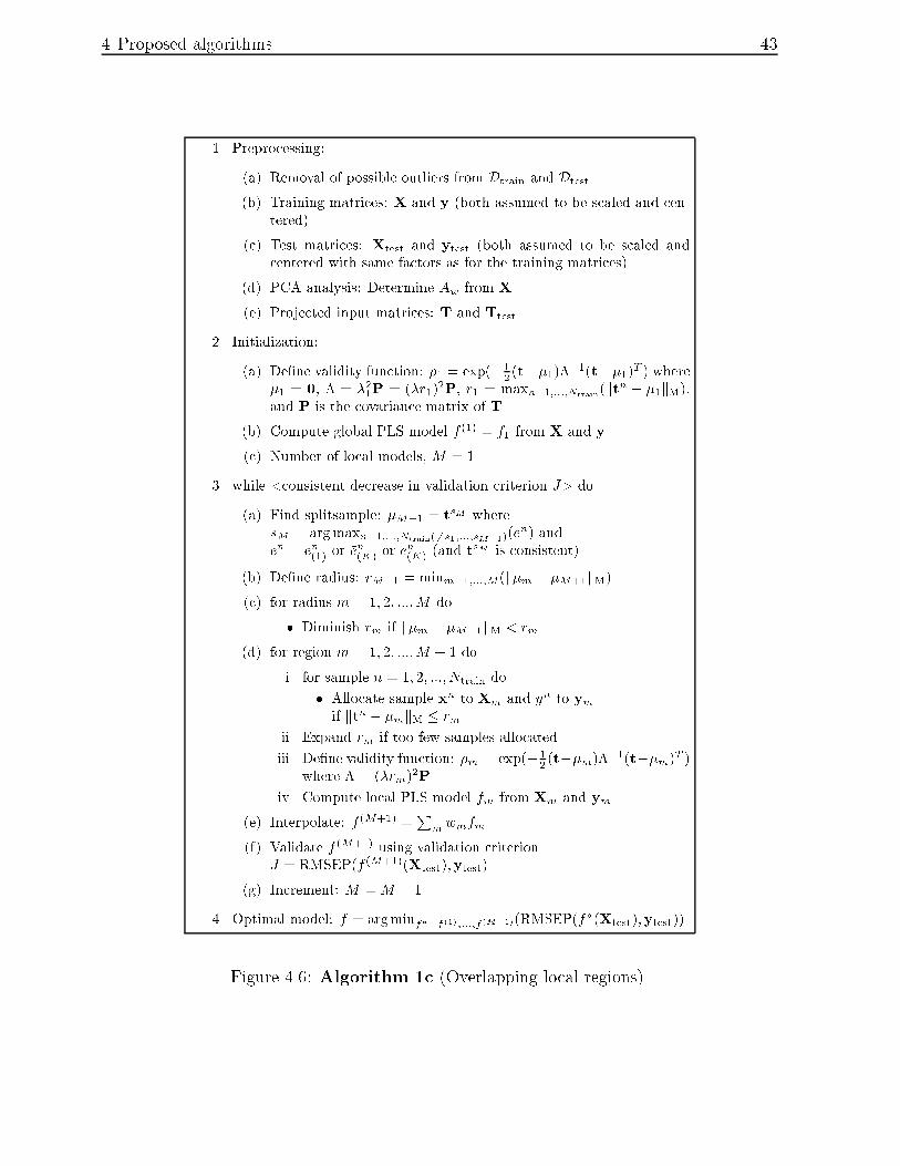
4 Proposed algorithms 43
1. Preprocessing:
(a) Removal of possible outliers from Dtrain and Dtest.
(b) Training matrices: X and y (both assumed to be scaled and cen-
tered).
(c) Test matrices: Xtest and ytest (both assumed to be scaled and
centered with same factors as for the training matrices).
(d) PCA analysis: Determine Aw from X.
(e) Projected input matrices: T and Ttest.
2. Initialization:
(a) De�ne validity function: �1 = exp(� 12(t��1)�
�1(t��1)T ) where
�1 = 0, � = �21P = (�r1)
2P, r1 = maxn=1;:::;Ntrain(ktn � �1kM),
and P is the covariance matrix of T.
(b) Compute global PLS model f (1) = f1 from X and y.
(c) Number of local models, M = 1.
3. while <consistent decrease in validation criterion J> do
(a) Find splitsample: �M+1 = tsM where
sM = argmaxn=1;:::;Ntrain(6=s1;:::;sM�1)(en) and
en = e
n
(1) or en
(K) or en
(K) (and tsM is consistent).
(b) De�ne radius: rM+1 = minm=1;:::;M(k�m � �M+1kM)
(c) for radius m = 1; 2; :::;M do
� Diminish rm if k�m � �M+1kM < rm.
(d) for region m = 1; 2; :::;M + 1 do
i. for sample n = 1; 2; :::; Ntrain do
� Allocate sample xn to Xm and yn to ym
if ktn � �mkM � rm.
ii. Expand rm if too few samples allocated.
iii. De�ne validity function: �m = exp(� 12(t��m)�
�1(t��m)T )
where � = (�rm)2P.
iv. Compute local PLS model fm from Xm and ym.
(e) Interpolate: f (M+1) =P
mwmfm.
(f) Validate f (M+1) using validation criterion
J = RMSEP(f (M+1)(Xtest);ytest).
(g) Increment: M =M + 1.
4. Optimal model: f = argminf�=f (1);:::;f (M�1)(RMSEP(f�(Xtest);ytest)).
Figure 4.6: Algorithm 1c (Overlapping local regions).
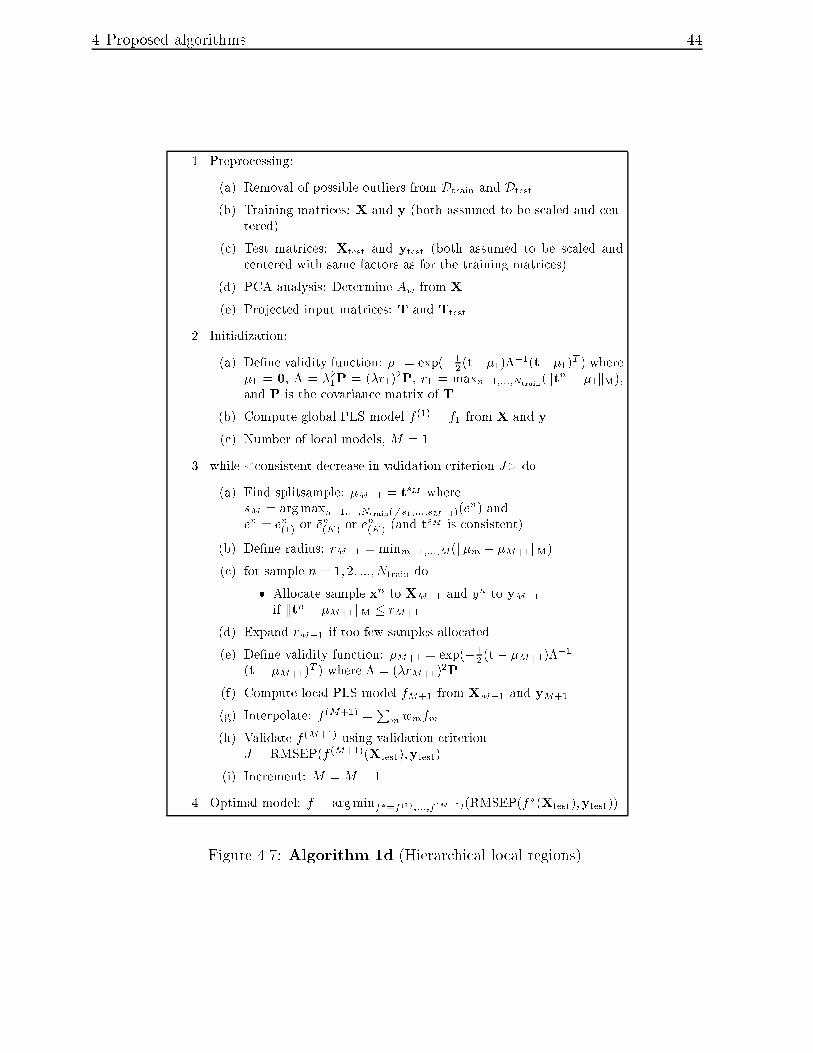
4 Proposed algorithms 44
1. Preprocessing:
(a) Removal of possible outliers from Dtrain and Dtest.
(b) Training matrices: X and y (both assumed to be scaled and cen-
tered).
(c) Test matrices: Xtest and ytest (both assumed to be scaled and
centered with same factors as for the training matrices).
(d) PCA analysis: Determine Aw from X.
(e) Projected input matrices: T and Ttest.
2. Initialization:
(a) De�ne validity function: �1 = exp(� 12(t��1)�
�1(t��1)T ) where
�1 = 0, � = �21P = (�r1)
2P, r1 = maxn=1;:::;Ntrain(ktn � �1kM),
and P is the covariance matrix of T.
(b) Compute global PLS model f (1) = f1 from X and y.
(c) Number of local models, M = 1.
3. while <consistent decrease in validation criterion J> do
(a) Find splitsample: �M+1 = tsM where
sM = argmaxn=1;:::;Ntrain(6=s1;:::;sM�1)(en) and
en = e
n
(1) or en
(K) or en
(K) (and tsM is consistent).
(b) De�ne radius: rM+1 = minm=1;:::;M(k�m � �M+1kM)
(c) for sample n = 1; 2; :::; Ntrain do
� Allocate sample xn to XM+1 and yn to yM+1
if ktn � �M+1kM � rM+1.
(d) Expand rM+1 if too few samples allocated.
(e) De�ne validity function: �M+1 = exp(� 12(t� �M+1)�
�1
(t� �M+1)T ) where � = (�rM+1)
2P.
(f) Compute local PLS model fM+1 from XM+1 and yM+1.
(g) Interpolate: f (M+1) =P
mwmfm.
(h) Validate f (M+1) using validation criterion
J = RMSEP(f (M+1)(Xtest);ytest).
(i) Increment: M =M + 1.
4. Optimal model: f = argminf�=f (1);:::;f (M�1)(RMSEP(f�(Xtest);ytest)).
Figure 4.7: Algorithm 1d (Hierarchical local regions).

4 Proposed algorithms 45
ConsistentConsistentConsistent
Error i.
Error ii.
Error iii.
Algorithm 1
e1c e2c e3c
e3nce2nce1nc
NotConsistent
NotConsistent
NotConsistent
Figure 4.8: The di�erent combinations of error measure and heuristic.
4.4 Evaluation on simple test examples
One of the di�culties with all the four versions of Algorithm 1 is the large number of
di�erent combinations of error measure and heuristic that are possible. The total number
is 6, as illustrated in �gure 4.8. In addition, the value of the external parameters K, the
number of neighboring samples, �, the degree of overlap, and Aw, the number of principal
components, must be determined for each combination. The procedure for �nding the
optimal combination is therefore very computationally demanding.
To examine the behavior of the four algorithms, they were all tested on a few simple
examples. These examples are described in the next section, together with the results of
Algorithm 1a. The most important results of the three other algorithms are given in
section 4.4.2.

4 Proposed algorithms 46
00.5
11.5
2
0
0.5
1
1.5
20
1
2
3
4
5
6
X1X2
Y
Surface of test function f1
Figure 4.9: Surface of f1.
4.4.1 Algorithm 1a
To investigate the properties of Algorithm 1a, the algorithm was �rst tested on the
smooth and simple low dimensional (P = 2) function
y = f1(x1; x2) = (x1)2 +
1
2(x2)
2 (4.6)
whose surface is illustrated in �gure 4.9.
The goal of this simple nonlinear example was just to illustrate that the principle of local
modeling is sensible, and that the algorithm worked. The number of input variables was
chosen to be 2, which provides simple three-dimensional plots of the relationship between
the variables.
All the samples of x1 and x2 were randomly drawn from a uniform [0,2] distribution.
Two training sets of 100 samples each and one test set of 500 samples were constructed.
One of the training sets was without noise on the output samples. To the yn's in the other
set, white noise, e � N(0; �2e) with �e = 0:5, corresponding to � 37 % (�e=S(y)) noise
level, was added. Noise was not added to the test set.
The same procedure was then repeated, but the number of samples in the two training
sets was now 300. In the test set it was still 500, though. The purpose was to investigate
what happens when the number of training samples increases. In all the tables the two
noiseless training sets are named 100 and 300, whereas the two noisy sets are named 100n
and 300n.

4 Proposed algorithms 47
Model 100 100n 300 300n
Linear 0.324 0.328 0.347 0.339
Quadratic 0.000 0.084 0.000 0.055
e1c 0.089 (7) 0.203 (5) * 0.061 (9) 0.177 (3)
e1nc 0.089 (7) 0.195 (3) 0.061 (9) 0.128 (8)
e2c 0.092 (7) 0.201 (5) * 0.058 (9) 0.145 (6)
e2nc 0.065 (9) 0.176 (7) 0.058 (9) 0.145 (6)
e3c 0.101 (6) 0.209 (6) * 0.053 (10) 0.145 (6)
e3nc 0.101 (6) 0.194 (4) 0.053 (10) 0.155 (8)
Table 4.1: RMSEP for di�erent models for approximating f1a.
Algorithm 1a was then run with �xed K = 5 and � = 12for the four di�erent data
sets and involving all 6 combinations. The results in RMSEP are given in table 4.1. First
of all, this table clearly shows, as was intended, that local linear modeling indeed decreases
the prediction error, compared to what a global linear model does. This hardly comes
as a surprise. Secondly, one observes that the generalization properties are better, both
for noiseless and noisy data sets, with 300 training samples than with only 100. Again,
a rather obvious result, since an increase in the number of samples will allow more local
models and also 'even out' the in�uence of noise in the samples. The third observation is
that the prediction error is larger for the noisy data sets than for the noiseless, when the
same test set is used. Something, which of course is as expected.
What is more interesting though, is to look at the estimation error. For noiseless data,
the RMSEE had approximately the same evolution, with regard to the order of magnitude,
as the RMSEP when M increased. For noisy data, the RMSEE was larger than RMSEP,
but the relative evolution was still the same. With 100 training samples, the RMSEE was
reduced from 0.604 (linear model) to 0.46�0.48 (best local linear models), and with 300
samples from 0.605 to 0.50�0.52. This corresponds to the noise level (0.5), and indicates
that no further improvement can be expected since only noise is left to be modelled. Thus,
the algorithm is able to withdraw as much information as possible from the noisy data,
which is an encouraging property. Another way of showing this is to compute the RMSE
between the noisy output training samples and the corresponding 'true' output samples.
This value was also approximately 0.5 for the best local linear models.
The best noiseless local linear model was e3nc, and the best based on noisy samples
was e1nc. The model surfaces are illustrated in �gure 4.10 and �gure 4.11 respectively.
These �gures can be compared with �gure 4.9.
aNumber of local models is given in parenthesis. An asterisk (*) means that the algorithm aborted
when no consistent sample was found, whereas a hash mark (#) means that it aborted due to fewer than
4 samples in a local region.
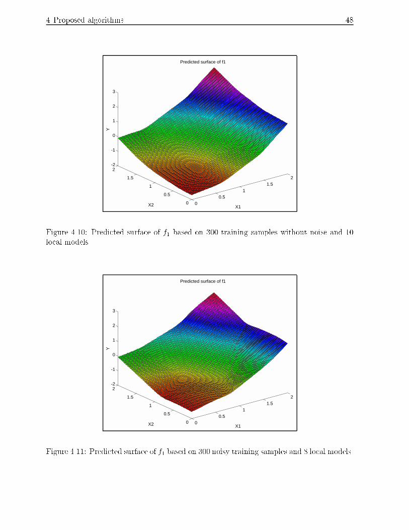
4 Proposed algorithms 48
00.5
11.5
2
0
0.5
1
1.5
2-2
-1
0
1
2
3
X1X2
Y
Predicted surface of f1
Figure 4.10: Predicted surface of f1 based on 300 training samples without noise and 10
local models.
00.5
11.5
2
0
0.5
1
1.5
2-2
-1
0
1
2
3
X1X2
Y
Predicted surface of f1
Figure 4.11: Predicted surface of f1 based on 300 noisy training samples and 8 local models.

4 Proposed algorithms 49
0 5 100.05
0.1
0.15
0.2
0.25
0.3
0.35
0.4
Number of local models
RM
SE
P
Error evolution
-4 -2 0 2 4-2.5
-2
-1.5
-1
-0.5
0
0.5
1
1.5
2
2.5
t1
t2
Model distribution
Figure 4.12: The model with lowest minimum RMSEP based on 300 training samples
without noise. (a) Evolution of RMSEP. (b) Distribution of local centers (x) in weighting
space.
The evolution of the RMSEP as M increases for the same two models is given in
�gure 4.12a and �gure 4.13a. These curves are typical of the general behavior of the
RMSEP. Often, at some stage, it slightly rises before decreasing again in the next step.
The illustrations on the right in these �gures show the distribution of the local centers �m,
i.e. splitsamples, in W . For a simple homogeneous function like f1, it is the best if they
are as evenly spread out in the input space as possible. As seen from the illustrations this
was indeed the case, which is another sensible property of Algorithm 1a.
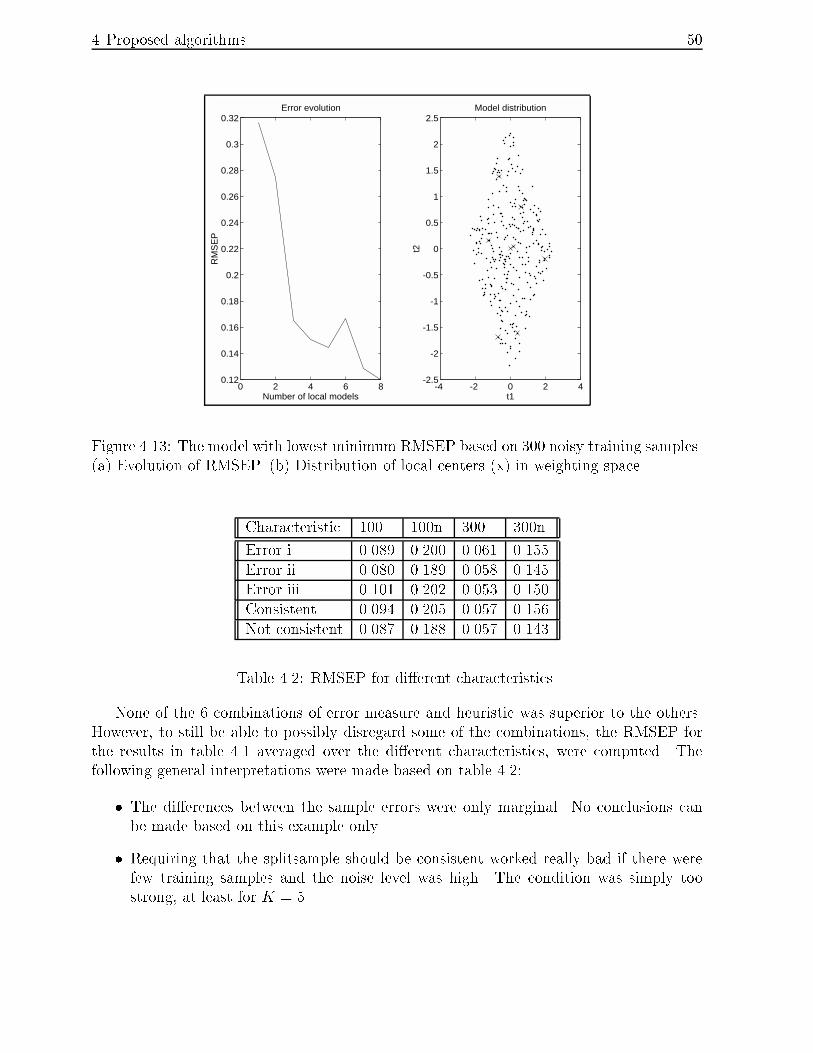
4 Proposed algorithms 50
0 2 4 6 80.12
0.14
0.16
0.18
0.2
0.22
0.24
0.26
0.28
0.3
0.32
Number of local models
RM
SE
P
Error evolution
-4 -2 0 2 4-2.5
-2
-1.5
-1
-0.5
0
0.5
1
1.5
2
2.5
t1
t2
Model distribution
Figure 4.13: The model with lowest minimum RMSEP based on 300 noisy training samples.
(a) Evolution of RMSEP. (b) Distribution of local centers (x) in weighting space.
Characteristic 100 100n 300 300n
Error i. 0.089 0.200 0.061 0.155
Error ii. 0.080 0.189 0.058 0.145
Error iii. 0.101 0.202 0.053 0.150
Consistent 0.094 0.205 0.057 0.156
Not consistent 0.087 0.188 0.057 0.143
Table 4.2: RMSEP for di�erent characteristics.
None of the 6 combinations of error measure and heuristic was superior to the others.
However, to still be able to possibly disregard some of the combinations, the RMSEP for
the results in table 4.1 averaged over the di�erent characteristics, were computed. The
following general interpretations were made based on table 4.2:
� The di�erences between the sample errors were only marginal. No conclusions can
be made based on this example only.
� Requiring that the splitsample should be consistent worked really bad if there were
few training samples and the noise level was high. The condition was simply too
strong, at least for K = 5.

4 Proposed algorithms 51
-1-0.5
00.5
1
-1
-0.5
0
0.5
1-2
-1
0
1
2
3
X1X2
Y
Surface of test function f2
Figure 4.14: Surface of f2.
The values of K and � were both �xed in the previous testing. However, to investigate
the consequences of varying values, K was �rst increased from 5 via 10 to 20. The result was
a more stable RMSEP evolution, although the minimum was at the same level. Then, the
consistency heuristic, with K = 3, was tested. Again, no improvements of the best results
in table 4.1 were observed. A large K will almost replace the consistency heuristic, since
the mean and median sample error will be computed over a larger region. The drawback
is that computation of the nearest neighboring samples will be slower. The value of �
was also changed from 12to both larger and smaller values. However, the e�ect was only
reduced prediction ability.
Algorithm 1a was then tested on a much more nonlinear function
y = f2(x1; x2) = (x1)3 � (x1)
2 �1
4x1 � x1x2 + 2(x2)
2 (4.7)
whose surface is illustrated in �gure 4.14.
The goal of this example was to illustrate that the algorithm is sensible also on highly
nonlinear problems.
All the samples of x1 and x2 were now drawn from a uniform [-1,1] distribution. Again a
noiseless test set of 500 samples and two training sets of 200 samples each, were constructed.
White noise, e � N(0; �2e) with �e = 0:5, was added to the output samples in one of the
training sets. This corresponds to a noise level (�e=S(y)) of 63 %, which is much, perhaps
too much. The noiseless training set is named 200, and the noisy set 200n in all the tables.

4 Proposed algorithms 52
Model 200 200n
Linear 0.764 0.762
Quadratic (x) 0.159 0.184
Cubic (x) 0.000 0.116
e1c 0.134 (8) # 0.438 (3) *
e1nc 0.120 (8) 0.221 (6)
e2c 0.170 (10) # 0.435 (3) *
e2nc 0.170 (10) # 0.201 (6)
e3c 0.169 (12) # 0.385 (3) *
e3nc 0.161 (12) 0.203 (6)
Table 4.3: RMSEP for di�erent models for approximating f2b.
The lowest RMSEP for di�erent models are given in table 4.3, for �xed K = 10 and
� = 12. Generally, local modeling vastly improved the prediction results compared to a
linear model, and also fared well against higher order polynomial models with cross-terms.
For the noiseless data set, the best local linear models were those using the sample
error of type i.. Probably because without noise on the training samples, there will be no
outliers, thus the single error approach will give a correct and undisturbed re�ection of
where the prediction is worst. Even though, the contrast to the other error measures was
still not signi�cant.
The number of local models was relatively large, and would have been even greater
had the training set been larger. As it was now, the algorithm aborted for almost every
combination. This because too few training samples were allocated to one class, but without
having reached the minimum RMSEP, indicating that additional improvement would have
been possible.
Figure 4.15 illustrates the model surface of the best local linear model, e1nc. If this
surface is compared to the original surface (�gure 4.14), one observes that although there
are di�erences, the general features of f2 are captured, so the approximation was not that
bad.
bSee table 4.1 for explanation of symbols.

4 Proposed algorithms 53
-1-0.5
00.5
1
-1
-0.5
0
0.5
1-3
-2
-1
0
1
2
3
X1X2
Y
Predicted surface of f2
Figure 4.15: Predicted surface of f2 based on training samples without noise and 8 local
models.
The evolution of the RMSEP and the distribution of the local centers �m in W , for
the same model, are given in �gure 4.16. Again, the local centers were well spread out
in the input space. This can be seen even better from �gure 4.17, where the weight,
wm(x), of each of the local models is illustrated as a function of input space position. A
comparison between the peaks in this illustration and the position of the local centers,
although rotated and stretched by the PCA, indicates that even though two splitsamples
have an almost identical position, the corresponding weight functions will peak apart from
each other because they are normalized.
The drawback with the noisy data set was that it was so noisy that the algorithm
aborted quickly if consistent splitsamples were required. Using the heuristic was therefore
impossible, at least for K = 10. The number of neighboring samples was then reduced to
5, which resulted in no abortions, and prediction results almost on the same level as those
obtained without the heuristic in table 4.3.
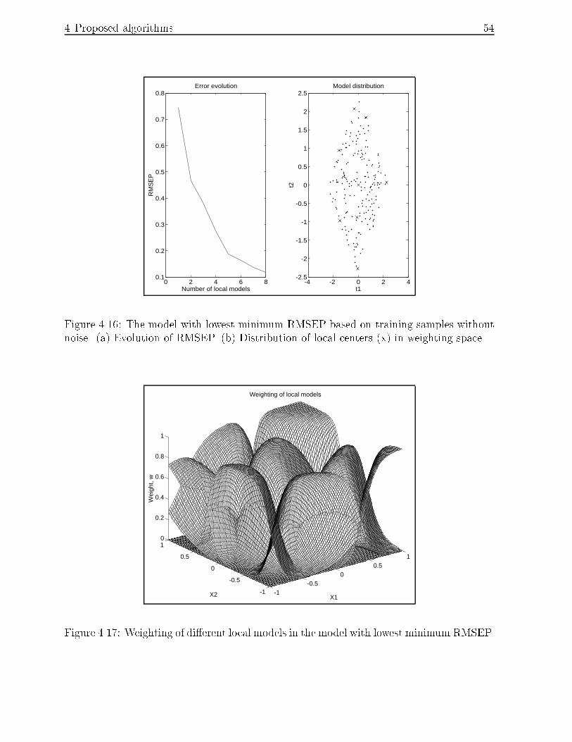
4 Proposed algorithms 54
0 2 4 6 80.1
0.2
0.3
0.4
0.5
0.6
0.7
0.8
Number of local models
RM
SE
P
Error evolution
-4 -2 0 2 4-2.5
-2
-1.5
-1
-0.5
0
0.5
1
1.5
2
2.5
t1t2
Model distribution
Figure 4.16: The model with lowest minimum RMSEP based on training samples without
noise. (a) Evolution of RMSEP. (b) Distribution of local centers (x) in weighting space.
-1-0.5
00.5
1
-1
-0.5
0
0.5
10
0.2
0.4
0.6
0.8
1
X1X2
Wei
ght,
w
Weighting of local models
Figure 4.17: Weighting of di�erent local models in the model with lowest minimum RMSEP.

4 Proposed algorithms 55
-1-0.5
00.5
1
-1
-0.5
0
0.5
1-3
-2
-1
0
1
2
3
X1X2
Y
Predicted surface of f2
Figure 4.18: Predicted surface of f2 based on noisy training samples and 6 local models.
When the algorithm did not pre-terminate, inspection of the RMSEE showed once more
that the noise level of 0.5 was reached at minimum RMSEP. The RMSEE was reduced
from 0.891 (linear model) to 0.50-0.52 (best local linear models). Although the data set
was very noisy, the model surface of the best local linear model, e2nc, is given in �gure 4.18
for completeness.
The most important conclusion that could be drawn from testing Algorithm 1a on
these two small examples was:
� The algorithm was a sensible approach in low dimensional problems.
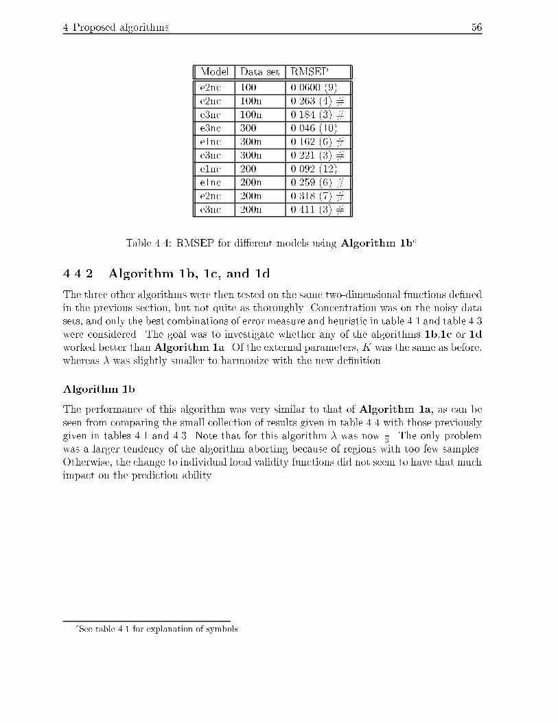
4 Proposed algorithms 56
Model Data set RMSEP
e2nc 100 0.0600 (9)
e2nc 100n 0.263 (4) #
e3nc 100n 0.184 (3) #
e3nc 300 0.046 (10)
e1nc 300n 0.162 (6) #
e3nc 300n 0.221 (3) #
e1nc 200 0.092 (12)
e1nc 200n 0.259 (6) #
e2nc 200n 0.318 (7) #
e3nc 200n 0.411 (3) #
Table 4.4: RMSEP for di�erent models using Algorithm 1bc.
4.4.2 Algorithm 1b, 1c, and 1d
The three other algorithms were then tested on the same two-dimensional functions de�ned
in the previous section, but not quite as thoroughly. Concentration was on the noisy data
sets, and only the best combinations of error measure and heuristic in table 4.1 and table 4.3
were considered. The goal was to investigate whether any of the algorithms 1b,1c or 1d
worked better than Algorithm 1a. Of the external parameters, K was the same as before,
whereas � was slightly smaller to harmonize with the new de�nition.
Algorithm 1b
The performance of this algorithm was very similar to that of Algorithm 1a, as can be
seen from comparing the small collection of results given in table 4.4 with those previously
given in tables 4.1 and 4.3. Note that for this algorithm � was now 13. The only problem
was a larger tendency of the algorithm aborting because of regions with too few samples.
Otherwise, the change to individual local validity functions did not seem to have that much
impact on the prediction ability.
cSee table 4.1 for explanation of symbols.

4 Proposed algorithms 57
0 2 4 60
0.5
1
1.5
2
2.5
3
3.5
4
4.5
5
Number of local models
RM
SE
P
Error evolution
0 5 100.3
0.35
0.4
0.45
0.5
0.55
0.6
0.65
0.7
0.75
0.8
Number of local models
RM
SE
P
Error evolution
Figure 4.19: Large jumps in the evolution of the RMSEP for Algorithm 1c. (a) 300n.
(b) 200n.
Algorithm 1c
The prediction ability was generally on the same level as for the �rst algorithm. A little
better for f1, but worse for the second function. However, the major drawback was the large
increase in RMSEP which occurs when the position of a new splitsample forces large regions
to diminish, because of the reduction of the radius in these regions. The corresponding local
models are then computed from far less samples than in the previous iteration. Typical
examples are given in �gure 4.19. This behavior makes the algorithm very unstable and
accidental, and not very robust, although the minimum RMSEP compared well to that of
Algorithm 1a.
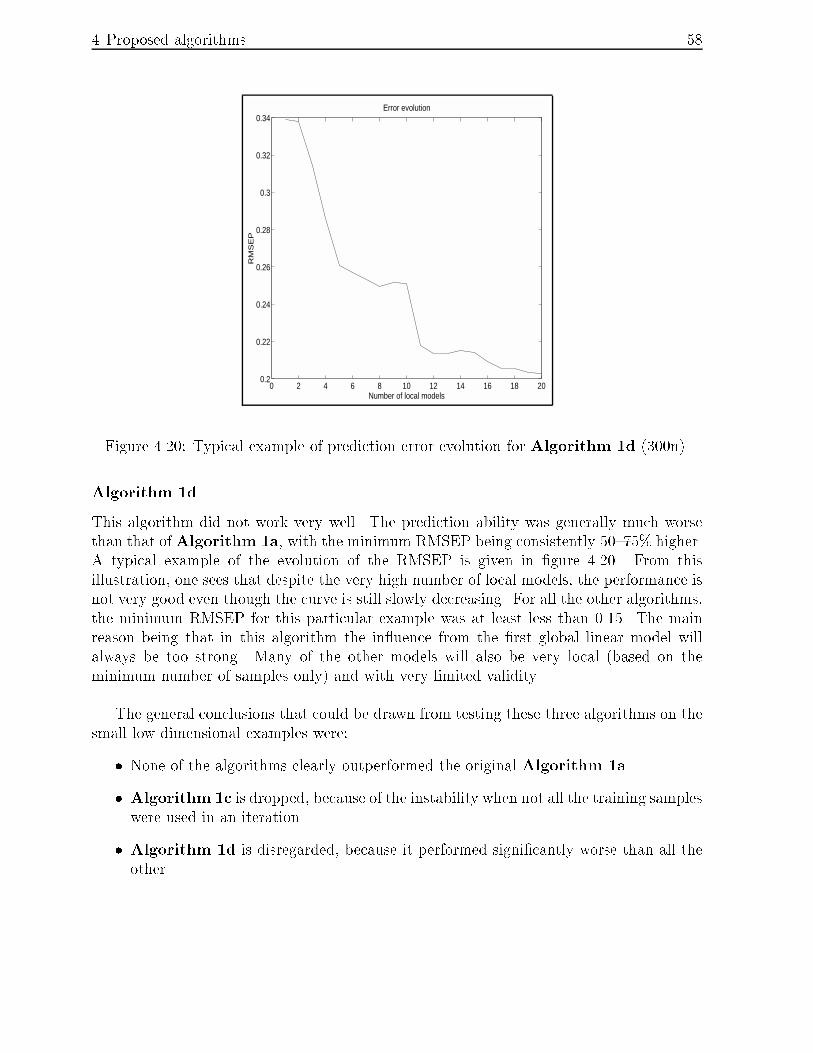
4 Proposed algorithms 58
0 2 4 6 8 10 12 14 16 18 200.2
0.22
0.24
0.26
0.28
0.3
0.32
0.34
Number of local models
RM
SE
P
Error evolution
Figure 4.20: Typical example of prediction error evolution for Algorithm 1d (300n).
Algorithm 1d
This algorithm did not work very well. The prediction ability was generally much worse
than that ofAlgorithm 1a, with the minimum RMSEP being consistently 50�75% higher.
A typical example of the evolution of the RMSEP is given in �gure 4.20. From this
illustration, one sees that despite the very high number of local models, the performance is
not very good even though the curve is still slowly decreasing. For all the other algorithms,
the minimum RMSEP for this particular example was at least less than 0.15. The main
reason being that in this algorithm the in�uence from the �rst global linear model will
always be too strong. Many of the other models will also be very local (based on the
minimum number of samples only) and with very limited validity.
The general conclusions that could be drawn from testing these three algorithms on the
small low dimensional examples were:
� None of the algorithms clearly outperformed the original Algorithm 1a.
� Algorithm 1c is dropped, because of the instability when not all the training samples
were used in an iteration.
� Algorithm 1d is disregarded, because it performed signi�cantly worse than all the
other.
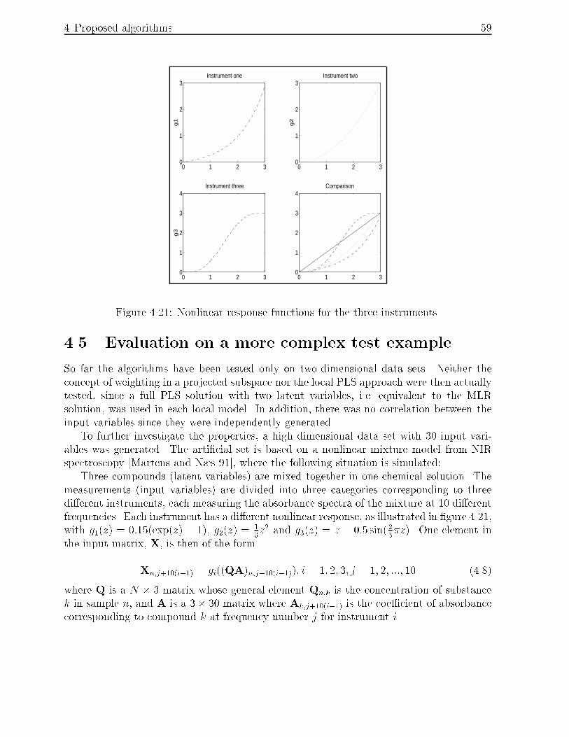
4 Proposed algorithms 59
0 1 2 30
1
2
3
g1
Instrument one
0 1 2 30
1
2
3
g2
Instrument two
0 1 2 30
1
2
3
4
g3
Instrument three
0 1 2 30
1
2
3
4Comparison
Figure 4.21: Nonlinear response functions for the three instruments.
4.5 Evaluation on a more complex test example
So far the algorithms have been tested only on two-dimensional data sets. Neither the
concept of weighting in a projected subspace nor the local PLS approach were then actually
tested, since a full PLS solution with two latent variables, i.e. equivalent to the MLR
solution, was used in each local model. In addition, there was no correlation between the
input variables since they were independently generated.
To further investigate the properties, a high dimensional data set with 30 input vari-
ables was generated. The arti�cial set is based on a nonlinear mixture model from NIR
spectroscopy [Martens and Næs 91], where the following situation is simulated:
Three compounds (latent variables) are mixed together in one chemical solution. The
measurements (input variables) are divided into three categories corresponding to three
di�erent instruments, each measuring the absorbance spectra of the mixture at 10 di�erent
frequencies. Each instrument has a di�erent nonlinear response, as illustrated in �gure 4.21,
with g1(z) = 0:15(exp(z) � 1), g2(z) =13z2 and g3(z) = z � 0:5 sin(2
3�z). One element in
the input matrix, X, is then of the form
Xn;j+10(i�1) = gi((QA)n;j+10(i�1)); i = 1; 2; 3; j = 1; 2; :::; 10 (4.8)
where Q is a N � 3 matrix whose general element Qn;k is the concentration of substance
k in sample n, and A is a 3� 30 matrix where Ak;j+10(i�1) is the coe�cient of absorbance
corresponding to compound k at frequency number j for instrument i.

4 Proposed algorithms 60
Model Algorithm 1a Algorithm 1b
Linear PLS (5 lv) 0.055
MLR (=PLS (30 lv)) 0.057
Quadratic PLS (10 lv) 0.036
Quadratic (60 lv) 0.039
Cubic PLS (17 lv) 0.030
Cubic (90 lv) 0.045
e1nc 0.030 (6) 0.037 (7)
e1c 0.038 (4) 0.032 (5)
e2nc 0.023 (6) 0.031 (7)
e2c 0.030 (6) 0.031 (7)
e3nc 0.034 (5) 0.038 (3)
e3c 0.038 (4) 0.034 (4)
Table 4.5: RMSEP for di�erent models for the spectrometry data setd.
The output variable is simply one of the compounds. Which one, is arbitrary since
all three are generated in the same way. The one, where the RMSEP and RMSEE for
an initial linear PLS model were largest, indicating most potential for improvement, was
chosen. This was number three, i.e. yn = Qn;3.
A training set of 150 and a test set of 50 samples were generated. All the elements in
both Q and A were randomly drawn from a uniform [0,1] distribution. In addition, 10 %
white noise was added to the 30 input variables in both the training and test set.
Both Algorithm 1a and 1b were �rst tested with � = 12and K = 5. The number
of principal components, Aw, in the weighting subspace W was 3, equaling the number
of compounds. The results in RMSEP are given in table 4.5. In the local modeling, the
number of latent variables in each local PLS model varied from 3 to 6.
The results clearly indicate that both local modeling algorithms improve the prediction,
with the lowest RMSEP being under half that of the linear PLS model. The main reason is
the nonlinearity in the data, which the linear PLS model was not able to model particularly
well, as seen from the slight curvature in �gure 4.22. With local modeling this curvature
is no longer present (�gure 4.23). Local modeling was also superior to 2nd and 3rd order
PLS (without cross terms).
dSee table 4.1 for explanation of symbols.
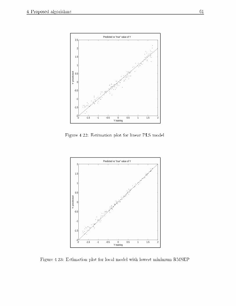
4 Proposed algorithms 61
-2 -1.5 -1 -0.5 0 0.5 1 1.5 2-2
-1.5
-1
-0.5
0
0.5
1
1.5
2
2.5
Y training
Y p
red
icte
d
Predicted vs "true" value of Y
Figure 4.22: Estimation plot for linear PLS model.
-2 -1.5 -1 -0.5 0 0.5 1 1.5 2-2
-1.5
-1
-0.5
0
0.5
1
1.5
2
Y training
Y p
red
icte
d
Predicted vs "true" value of Y
Figure 4.23: Estimation plot for local model with lowest minimum RMSEP.

4 Proposed algorithms 62
For Algorithm 1a, � was changed to 14, 3
4, and 1 without improving the results at
all. For � = 12, K = 3 and K = 10 was also tested. Again the results were generally
worse compared to those in table 4.5. For Algorithm 1b, a change in the value of � to34resulted in much higher RMSEP, whereas the results for � = 1
3and 1
4were generally on
the same level as those in the table. This is to be expected since the radii rm, due to the
way of scaling the axes in W , are very often larger than 1 which corresponds to the �xed
validity function used in Algorithm 1a. The optimal value of � will then be smaller for
Algorithm 1b than for the �rst algorithm.
One di�erence between the two algorithms was that over�tting was more of a problem
using Algorithm 1b than Algorithm 1a. Generally, the RMSEE was lower, but the
RMSEP was higher for the former algorithm compared to the latter one. Thus, Algorithm
1b is able to better approximate the training samples, probably because of the use of
individual validity functions. It must be said though, that the di�erence was not much.
The RMSEE was reduced from 0.049 (linear PLS) to 0.020-0.024 in both cases.
The average correlation (see appendix B.1) between the di�erent input variables was
0.81, which indicates strongly correlated variables. In comparison the average correlation
for the arti�cial data sets generated from f1 and f2 was between 0.01 and 0.12.
The main conclusions that could be drawn from this high dimensional problem with
correlated input variables were:
� Both local modeling algorithms worked much better than linear PLS.
� The concept of low dimensional weighting space and local PLS modeling seemed
fruitful even when P was large.
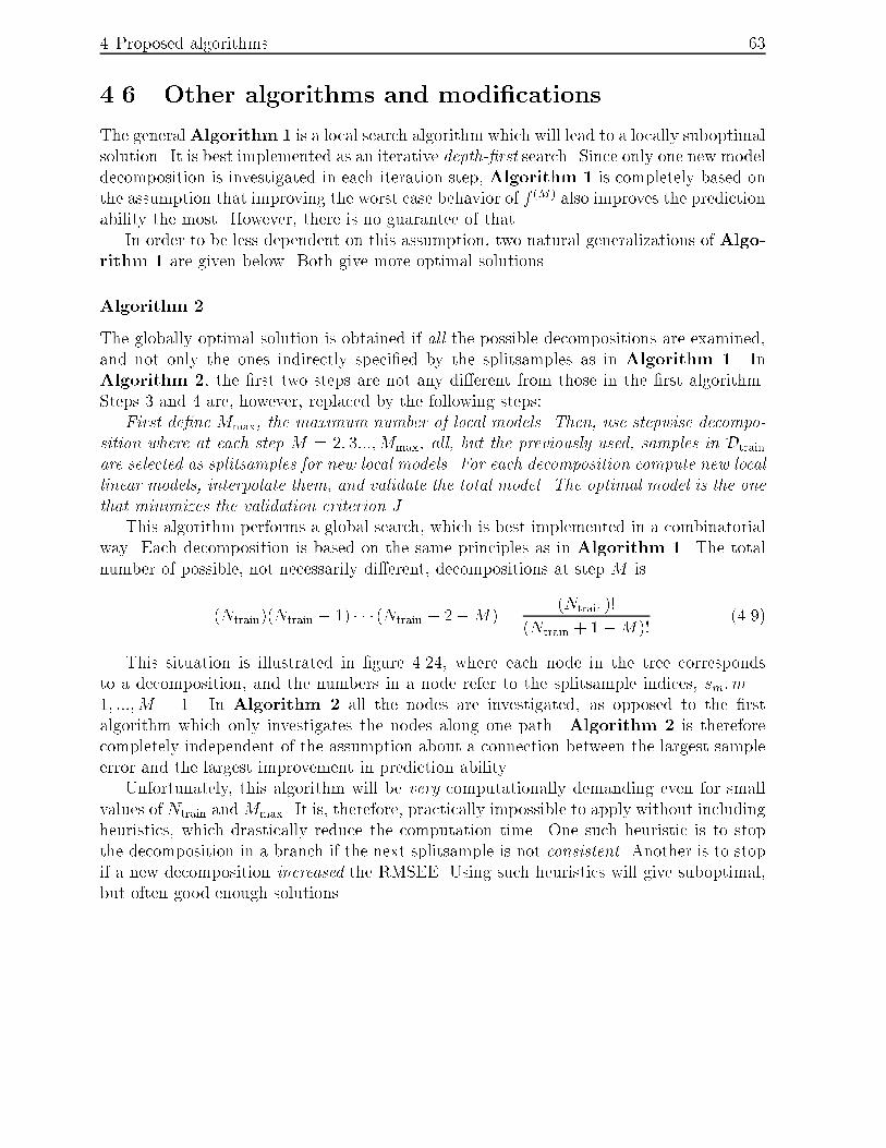
4 Proposed algorithms 63
4.6 Other algorithms and modi�cations
The generalAlgorithm 1 is a local search algorithm which will lead to a locally suboptimal
solution. It is best implemented as an iterative depth-�rst search. Since only one new model
decomposition is investigated in each iteration step, Algorithm 1 is completely based on
the assumption that improving the worst case behavior of f (M) also improves the prediction
ability the most. However, there is no guarantee of that.
In order to be less dependent on this assumption, two natural generalizations of Algo-
rithm 1 are given below. Both give more optimal solutions.
Algorithm 2
The globally optimal solution is obtained if all the possible decompositions are examined,
and not only the ones indirectly speci�ed by the splitsamples as in Algorithm 1. In
Algorithm 2, the �rst two steps are not any di�erent from those in the �rst algorithm.
Steps 3 and 4 are, however, replaced by the following steps:
First de�ne Mmax, the maximum number of local models. Then, use stepwise decompo-
sition where at each step M = 2; 3:::;Mmax, all, but the previously used, samples in Dtrain
are selected as splitsamples for new local models. For each decomposition compute new local
linear models, interpolate them, and validate the total model. The optimal model is the one
that minimizes the validation criterion J.
This algorithm performs a global search, which is best implemented in a combinatorial
way. Each decomposition is based on the same principles as in Algorithm 1. The total
number of possible, not necessarily di�erent, decompositions at step M is
(Ntrain)(Ntrain � 1) � � � (Ntrain + 2�M) =(Ntrain)!
(Ntrain + 1�M)!(4.9)
This situation is illustrated in �gure 4.24, where each node in the tree corresponds
to a decomposition, and the numbers in a node refer to the splitsample indices, sm; m =
1; :::;M � 1. In Algorithm 2 all the nodes are investigated, as opposed to the �rst
algorithm which only investigates the nodes along one path. Algorithm 2 is therefore
completely independent of the assumption about a connection between the largest sample
error and the largest improvement in prediction ability.
Unfortunately, this algorithm will be very computationally demanding even for small
values of Ntrain andMmax. It is, therefore, practically impossible to apply without including
heuristics, which drastically reduce the computation time. One such heuristic is to stop
the decomposition in a branch if the next splitsample is not consistent. Another is to stop
if a new decomposition increased the RMSEE. Using such heuristics will give suboptimal,
but often good enough solutions.

4 Proposed algorithms 64
:::
M=1
M=2
M=3
M=4
1 2 N
1,2 1,3 1,N
1,2,3 1,2,4 1,2,N
......
....
......
Figure 4.24: Possible decompositions based on the training samples.
Algorithm 3
This algorithm lies somewhere between the other two, since an extended local search is
performed. Steps 1, 2, and 4 are all unaltered, but the repeated step (3) in Algorithm 1
is now changed as follows:
First choose the L samples, 1 � L � Ntrain + 1 �M , of all the Ntrain + 1 �M non-
selected samples having the largest sample error of type i., ii., or iii. as candidates for
the splitsample. For all these candidates, decompose the input space, compute new local
linear models and interpolate them. Select, as splitsample, the one of the candidates whose
decomposition and corresponding total model, f(M+1)l , gives the smallest RMSEE. Continue
with that total model, f (M+1) = f
(M+1)l , in the validation.
Algorithm 3 is less sensitive to the assumption about prediction improvement. This
because the decompositions from the L largest sample errors, and not only the largest, are
investigated in each iteration step. Therefore, the algorithm will be more computationally
demanding than Algorithm 1, but obviously faster than Algorithm 2. Again, heuristics
such as requiring consistent candidate samples will speed up the algorithm. As the �rst
algorithm, Algorithm 3 is best implemented as an iterative depth-�rst search.
In the limit L = Ntrain + 1 �M , the solution is one-step-ahead optimal in the sense
that it is optimal in that iteration step, since all possible decompositions are considered.
In �gure 4.24 that corresponds to looking at all the nodes in the next level of a subtree,
before deciding which node to enter. In the other special case L = 1, Algorithm 3 is
simply reduced to Algorithm 1.

4 Proposed algorithms 65
Although both of these two generalizations, of the �rst algorithm, most likely will give
slightly better solutions in terms of prediction ability, they were not implemented because
of their much higher computational demands. In the rest of this thesis all additional
testing and discussion is therefore related to Algorithm 1. The other two algorithms are
not considered any further.
A modi�cation of the strategy for determining the splitsample is then proposed.
Strategy 2
First compute the di�erent local RMSEE of the M local regions, using only local samples in
the computation. De�ne the region with the largest local RMSEE as the region of splitting.
Select the splitsample as the sample having the largest sample error of type i.,ii. or iii.,
under the condition that this sample is located within the region of splitting.
This strategy can be seen as a local version of strategy 1, with the search for a split-
sample restricted to a local region. However, the main purpose is to preserve an as equal
as possible degree of local linearity in the di�erent regions, measured in terms of local RM-
SEE. This principle gives a total model, f , with an approximately equally good prediction
ability everywhere in the input hyperspace, which is often desirable.
To investigate this strategy, Algorithm 1a was again tested on the two low dimensional
functions, but now with strategy 2 as the way of determining the splitsample. The results
are given in table 4.6 and 4.7.
Model 100 100n 300 300n
e1c 0.122 (6) * 0.303 (3) * 0.062 (9) 0.174 (6) *
e1nc 0.122 (6) # 0.195 (3) 0.062 (9) 0.133 (5)
e2c 0.085 (7) 0.215 (4) * 0.061 (9) 0.240 (5) *
e2nc 0.061 (9) 0.187 (7) # 0.061 (9) 0.159 (8)
e3c 0.101 (6) 0.239 (3) * 0.063 (8) 0.174 (3)
e3nc 0.101 (6) 0.187 (5) # 0.063 (8) 0.143 (7)
Table 4.6: RMSEP for di�erent models for approximating f1 (strategy 2)e.
eSee table 4.1 for explanation of symbols.

4 Proposed algorithms 66
Model 200 200n
e1c 0.180 (6) # 0.438 (3) *
e1nc 0.141 (8) # 0.259 (5)
e2c 0.142 (12) # 0.435 (3) *
e2nc 0.142 (12) # 0.276 (4)
e3c 0.177 (9) # 0.385 (3) *
e3nc 0.170 (12) 0.291 (5) #
Table 4.7: RMSEP for di�erent models for approximating f2 (strategy 2)f .
Characteristic 100 100n 300 300n 200 200n
Strategy 1 0.091 0.197 0.057 0.150 0.155 0.332
Strategy 2 0.101 0.225 0.062 0.174 0.160 0.355
Table 4.8: RMSEP for di�erent strategies.
These tables correspond to table 4.1 and 4.3 for strategy 1. To be better able to compare
the two strategies, the RMSEP for the results in the four tables averaged over the strategies
were computed.
As seen from table 4.8 there was only one conclusion:
� Strategy 2 was worse than strategy 1, and is therefore disregarded.
fSee table 4.1 for explanation of symbols.

5
Case studies
This chapter describes a set of case studies that have been carried out in order to test the
new local modeling algorithms on well-known data sets, and to compare them with other
modeling techniques.
5.1 Introduction
So far the algorithms and their properties have only been investigated using specially
designed and arti�cially generated data sets. But do they behave any di�erently when
tested on real world examples? Another important question is, how well do the local
modeling algorithms perform compared to other nonlinear modeling techniques? These
two questions will be addressed in this chapter.
Comparisons between di�erent modeling techniques and algorithms are always di�cult,
as no technique will constantly outperform all the others on whatever data set imaginable.
Usually, algorithms are designed for a special modeling purpose and will work satisfactory
on these kind of problems. A good example is PLS, which works very well in NIR (near
infrared) spectroscopy where the number of input variables (i.e. wavelengths) is very high
(often P > 100), the size of the training set is small, and the variables are highly correlated.
On more lower dimensional and larger data sets though, other modeling techniques may
perform better than PLS.
Other factors that in�uence the performance of the di�erent techniques are:
Validation criterion. The choice of validation criterion (see section 2.1.4), which is the
measure of performance, can heavily in�uence the results and thereby the interpreta-
tions of what constitutes a successful algorithm. Running the same set of case studies
with another criterion may alter the rank between the algorithms.
67

5 Case studies 68
External parameter values. Di�erent algorithms often require a number of external pa-
rameters which have to be adjusted and tuned. Often, a small change in the param-
eter values can lead to very di�erent results. The higher this number of parameters
is, the more time is spent searching for an optimal combination. A parameter set is
also domain speci�c, as di�erent problems require di�erent sets of parameters. When
comparing algorithms, �nding a suitable set of parameter values should be given the
highest priority.
Computation time. Two aspects are involved here, the actual running time of the al-
gorithm and the time spent searching for optimal parameter values. To ensure a
comparable level between the algorithms tested, they should all be run and pro-
grammed on the same computer. In addition, equal time should be used on all the
algorithms when trying to �nd an optimal set of parameter values. Unfortunately,
none of this is grati�ed in the case studies, since it is mostly referred to the work of
others, except when giving the results of the proposed algorithms.
The conclusion is that care should always be taken when doing comparative studies of
di�erent algorithms. The results will not necessarily give you the absolute truth about the
performance of the techniques, only some ideas of the behavior. Be also aware that the
results are only valid for the particular data sets. Further extrapolation and generalization
beyond these should be done with extreme care.
5.2 Organization
To simplify comparisons between di�erent data sets, the results are given as normalized
root mean square error (NRMSE), which, unlike RMSE, is a relative and not absolute
measure of performance de�ned by
NRMSE =
qPNn=1 (y
n � �yn)2qPN
n=1 (yn � y)
2=
RMSEq1N
PNn=1 (y
n � y)2�
RMSE
S(y)(5.1)
If NRMSE is zero the prediction is perfect, whereas a value equal to 100% is equivalent to
using the average, y, as the predictor.
The local modeling algorithms were tested on four di�erent data sets, all of which have
previously been used by others when investigating di�erent modeling techniques. The
�rst one is generated from a simulation of a chemical catalytic reactor. The second is
obtained from the dynamics of a hydraulic industrial robot. Whereas the last two are
taken from the �eld of NIR spectroscopy, where water content in meat and sti�ness in
polymers are to be estimated, respectively. In all the data sets there is an anticipated
nonlinear relationship between the input and output variables which linear methods might
have problems identifying. The data sets are quite di�erent regarding the number of
training samples and input variables, the noise level, and the correlation of input variables
as shown in table 5.1.

5 Case studies 69
Data set # of training samples # of input variables Noise level Correlation
Reactor high (700) medium (5) zero low
Robot high (800) low (3) medium low
Meat low (70) very high (100) ? high
Polymer low (47) very high (138) ? high
Table 5.1: A rough characterization of the experimental data sets.
Based on the experiences with the arti�cially generated data sets in chapter 4, the case
studies were organized as follows regarding the value of the external parameters K, �, and
A, the type of sample error, and inclusion of the heuristic:
� Of the local PLS modeling algorithms, only Algorithm 1a and 1b were tested.
� All the types of sample error; single, mean, and median were analyzed for both
algorithms.
� The number of neighboring samples, K, was not much investigated. Instead, K was
given a reasonable value proportional to the size of the training set. This value was
then kept �xed after the initial choice, mostly because the computation of the nearest
neighboring samples was computational demanding and the time was limited.
� The degree of smoothing between the local models, �, was given an initial value of12, and then, more �nely tuned both upwards and downwards for the models with
initially the lowest minimum NRMSEP.
� The number of latent variables, Aw, in the projected input subspaceW was �xed, and
the e�ect of changing it was not investigated. The value was either 3 or 4 depending
on the di�erence in eigenvalue for the principal components.
� The consistency heuristic was included, but only together with a smaller value of K
than the initial choice.
� The NRMSEP values shown in the tables are the minimum values. Only the three
models with the lowest NRMSEP are displayed.
This process was repeated for all of the four data sets.
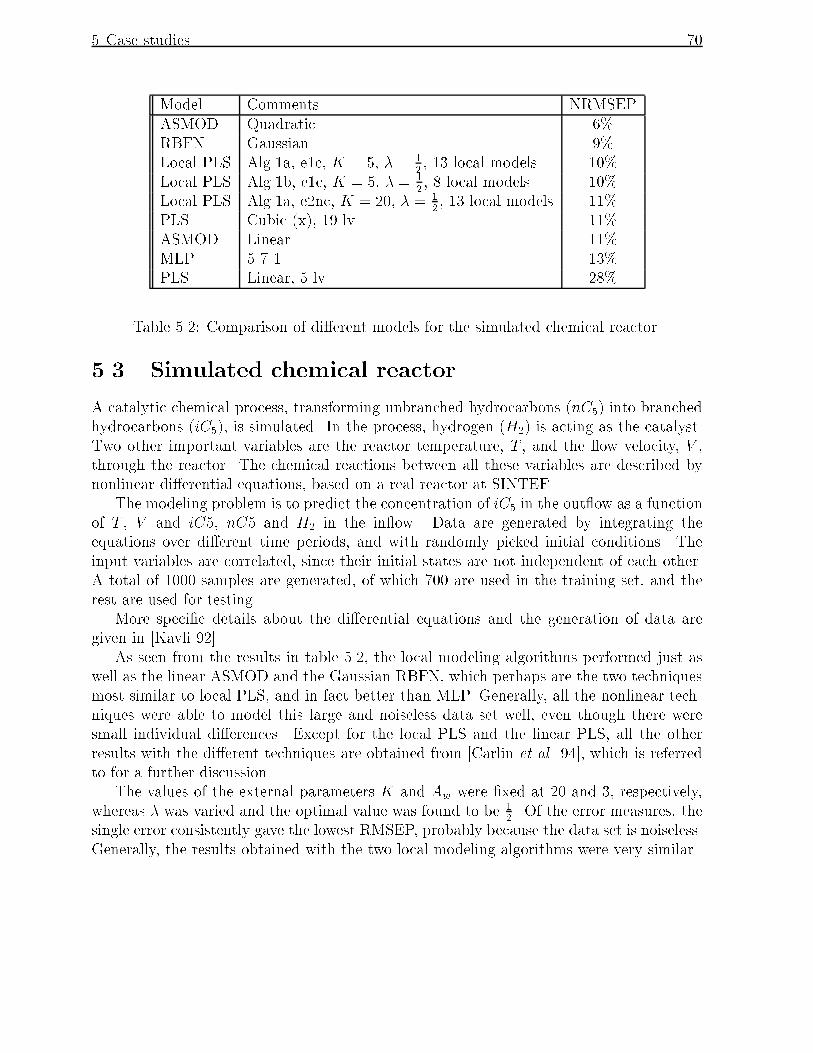
5 Case studies 70
Model Comments NRMSEP
ASMOD Quadratic 6%
RBFN Gaussian 9%
Local PLS Alg.1a, e1c, K = 5, � = 12, 13 local models 10%
Local PLS Alg.1b, e1c, K = 5, � = 12, 8 local models 10%
Local PLS Alg.1a, e2nc, K = 20, � = 12, 13 local models 11%
PLS Cubic (x), 19 lv 11%
ASMOD Linear 11%
MLP 5-7-1 13%
PLS Linear, 5 lv 28%
Table 5.2: Comparison of di�erent models for the simulated chemical reactor.
5.3 Simulated chemical reactor
A catalytic chemical process, transforming unbranched hydrocarbons (nC5) into branched
hydrocarbons (iC5), is simulated. In the process, hydrogen (H2) is acting as the catalyst.
Two other important variables are the reactor temperature, T , and the �ow velocity, V ,
through the reactor. The chemical reactions between all these variables are described by
nonlinear di�erential equations, based on a real reactor at SINTEF.
The modeling problem is to predict the concentration of iC5 in the out�ow as a function
of T , V and iC5, nC5 and H2 in the in�ow. Data are generated by integrating the
equations over di�erent time periods, and with randomly picked initial conditions. The
input variables are correlated, since their initial states are not independent of each other.
A total of 1000 samples are generated, of which 700 are used in the training set, and the
rest are used for testing.
More speci�c details about the di�erential equations and the generation of data are
given in [Kavli 92].
As seen from the results in table 5.2, the local modeling algorithms performed just as
well as the linear ASMOD and the Gaussian RBFN, which perhaps are the two techniques
most similar to local PLS, and in fact better than MLP. Generally, all the nonlinear tech-
niques were able to model this large and noiseless data set well, even though there were
small individual di�erences. Except for the local PLS and the linear PLS, all the other
results with the di�erent techniques are obtained from [Carlin et al. 94], which is referred
to for a further discussion.
The values of the external parameters K and Aw were �xed at 20 and 3, respectively,
whereas � was varied and the optimal value was found to be 12. Of the error measures, the
single error consistently gave the lowest RMSEP, probably because the data set is noiseless.
Generally, the results obtained with the two local modeling algorithms were very similar.

5 Case studies 71
Model Comments NRMSEP
ASMOD Quadratic 15%
LSA Linear 17%
ASMOD Linear 17%
RBFN Gaussian 19%
MLP 3-20-1 23%
PLS Cubic (x), 10 lv 26%
Local PLS (=MLR) Alg.1a, e2c, K = 5, � = 12, 7 local models 27%
Local PLS (=MLR) Alg.1a, e2nc, K = 20, � = 14, 7 local models 27%
Local PLS (=MLR) Alg.1b, e3c, K = 5, � = 13, 7 local models 27%
PLS (=MLR) Linear, 3 lv 63%
Table 5.3: Comparison of di�erent models for the hydraulic robot manipulator.
5.4 Hydraulic robot manipulator
The movements of an industrial hydraulic robot manipulator are investigated. Such ma-
nipulators have often su�ered from the lack of good dynamic models, due to nonlinear
hydrodynamic e�ects involved in the hydraulic components. The goal is to �nd an empiri-
cal model, describing the servo valve control signal, (u), as a function of the joint position
(q), velocity ( q), and acceleration (�q). A more complete description of this experiment can
be found in [Kavli 92].
Approximately 40000 samples are generated by sampling corresponding values of u and
q, as the manipulator is moving along a randomly generated trajectory. Values of q and �q
are then computed by low pass �ltering and numerical di�erentiations. A linear model is
subtracted from the data, leaving mainly nonlinear dependencies. Of the 40000 samples,
a training set of 800 and a test set of 200 samples were randomly picked. Note that this
training set corresponds to samples 1 to 800, and this test set to samples 801 to 1000 of what
is described as the independent test set in other articles [Kavli 92, Johansen and Foss 93].
This reduction was done because of limited time and computer resources. The results
obtained with these subsets should still be comparable to those using the large test set and
a training set of 8000 samples, because the number of samples was still fairly high and the
samples were well distributed in the input space.
The various results with di�erent techniques are given in table 5.3, where the result
for the LSA algorithm is taken from [Johansen and Foss 93] and the rest, except those for
the local and linear PLS, are obtained from [Carlin et al. 94]. For this data set, the local
PLS (or rather local MLR since P = 3 ) algorithms were outperformed by the other local
methods (LSA, ASMOD, RBFN). One reason is possibly that only 5-7 local models were
included in the best local PLS, which is few compared to the 10-13 for the reactor data
set. Why the minimum NRMSEP was reached after so few models is uncertain. There
should still have been room for improvement since applying the consistency heuristic with
K = 20 did not change the results very much. Practically all the suggested splitsamples

5 Case studies 72
were indeed consistent, indicating large error surfaces having the same sign.
The best local PLS model is plotted in �gure 5.1. The graph shows the control signal
(u) as a function of joint speed and acceleration, with the joint in the center position i.e.
q=0. The best model, with half as large value of �, is in comparison plotted in �gure 5.2.
Note how piecewise this model is since the smoothing parameter was very small. The
variation of � did not signi�cantly improve the prediction, as a NRMSEP of at least 30%
was always obtained regardless of the degree of smoothing.
-6-4
-20
24
6
x 104
-4
-2
0
2
4
x 105
-1000
-500
0
500
1000
SpeedAcceleration
Con
trol
, U
Predicted surface of U
Figure 5.1: Predicted surface of u based on 7 local models, with � = 12(e2c).
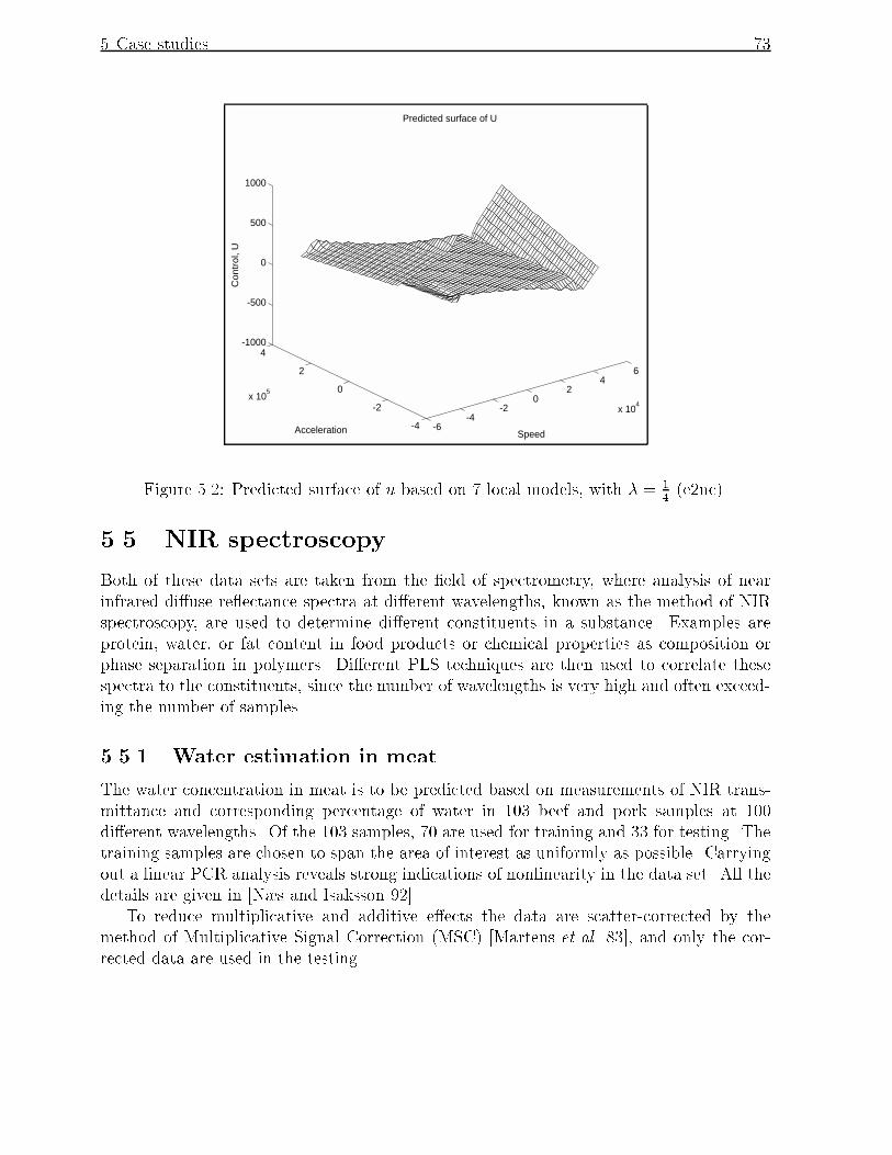
5 Case studies 73
-6-4
-20
24
6
x 104
-4
-2
0
2
4
x 105
-1000
-500
0
500
1000
SpeedAcceleration
Con
trol
, U
Predicted surface of U
Figure 5.2: Predicted surface of u based on 7 local models, with � = 14(e2nc).
5.5 NIR spectroscopy
Both of these data sets are taken from the �eld of spectrometry, where analysis of near
infrared di�use re�ectance spectra at di�erent wavelengths, known as the method of NIR
spectroscopy, are used to determine di�erent constituents in a substance. Examples are
protein, water, or fat content in food products or chemical properties as composition or
phase separation in polymers. Di�erent PLS techniques are then used to correlate these
spectra to the constituents, since the number of wavelengths is very high and often exceed-
ing the number of samples.
5.5.1 Water estimation in meat
The water concentration in meat is to be predicted based on measurements of NIR trans-
mittance and corresponding percentage of water in 103 beef and pork samples at 100
di�erent wavelengths. Of the 103 samples, 70 are used for training and 33 for testing. The
training samples are chosen to span the area of interest as uniformly as possible. Carrying
out a linear PCR analysis reveals strong indications of nonlinearity in the data set. All the
details are given in [Næs and Isaksson 92].
To reduce multiplicative and additive e�ects the data are scatter-corrected by the
method of Multiplicative Signal Correction (MSC) [Martens et al. 83], and only the cor-
rected data are used in the testing.

5 Case studies 74
Model Comments NRMSEP
MLP 8 lv, 8-3-1 9.7%
LWR 3 lv, K = 30 9.9%
MLP 50-10-1 10.6%
Local PLS Alg.1a, e2c, K = 3, � = 12, 3 local models 11.2%
PCR Linear, 8 lv 11.7%
Local PLS Alg.1a, e2nc, K = 5, � = 12, 4 local models 12.2%
Local PLS Alg.1b, e2c, K = 3, � = 12, 2 local models 12.4%
PLS Linear, 6 lv 13.1%
Table 5.4: Comparison of di�erent models for water estimation in meat.
Di�erent results for this data set are given in table 5.4. The results for LWR, PCR,
and MLP are obtained from [Næs and Isaksson 92] and [Næs et al. 93].
At �rst sight, the local algorithms seemed to improve the prediction. However, the
three results reported in the table were almost the only combinations of parameter values
that lead to a decrease in the NRMSP. For most of the other combinations, over�tting was
the outcome. Even increasing the smoothing between the local models by using a large
value of �, because of high dimensional data, did not help. The conclusion was that the
improvements were unreliable, maybe just the result of a lucky division of the training
samples and not part of a general tendency.
The reason is probably a combination of many things. At the minimum NRMSEP for
linear PLS, the corresponding NRMSEE was over 19%, i.e. much higher than the NRMSEP,
indicating that any closer �t to the training samples is very likely to increase the NRMSEP.
The small number of training samples made any nonlinear �t di�cult, as the number of local
models could only be 3�5, before the local PLS algorithms aborted as the result of too few
samples in a region. The question is also what really is a signi�cant nonlinear relationship
in a 100 dimensional space? Perhaps using this kind of local modeling approach on such
an extremely high dimensional problem was an overkill. Applying a nonlinear technique
on an almost linear problem can lead to less accurate predictions.
When running the local PLS algorithms, 10 latent variables were the upper limit in
each local model. The optimal number was manually selected, by investigating the plot
of residual sums of squares from cross-validation. However, virtually no restrictions were
put on the number of samples per latent variable. Often a local PLS model was computed
using e.g. 10 samples and 4�6 latent variables. The number of principal components in the
weighting subspace W was 3.
Note that the linear PCR prediction result was better than that of the linear PLS. A
relevant question, which has not been investigated, is whether using PCR as local modeling
technique instead of PLS would improve the predictions.

5 Case studies 75
Model Comments NRMSEP
MLP 138-25-1 9.3%
Local PLS Alg.1a, e2c, K = 3, � = 12, 2 local models 10.6%
Local PLS Alg.1b, e2c, K = 3, � = 12, 2 local models 10.8%
Local PLS Alg.1a, e1nc, K = 5, � = 12, 3 local models 12.3%
PLS Linear, 14 lv 13.3%
PCR Linear, 21 lv 13.5%
Table 5.5: Comparison of di�erent models for sti�ness estimation in polymer.
5.5.2 Sti�ness estimation in polymer
The goal is to predict the �ex modulus (sti�ness) of polyurethane elastomers on the basis
of the NIR spectra at 138 di�erent wavelengths. The data set contains a total of 90 spectra,
of which 47 form the training set and the remaining 43 serve as the test set. The samples
in the test set are chosen such that the values of the �ex modulus are within the range
of the values in the training set. Further details regarding this data set can be found in
[Miller and Eichinger 91].
Again, the data are MSC-corrected to reduce multiplicative and additive e�ects. As was
the case with the meat samples, linear PLS analysis shows a possible nonlinear relationship
between the input variables and the sti�ness [Miller and Eichinger 91].
Various results for this data set are presented in table 5.5. The result with MLP is
obtained from [Næs et al. 93]. Unfortunately, the same di�culties were present in this NIR
data set as in the previous one. Over�tting occurred at once for almost all combinations
of parameters in the local PLS algorithms, only 2-3 local models could be computed as the
algorithms aborted very quickly, improving the result of the linear PLS was hard etc. The
reasons for this behavior are the same as they were for the meat samples. The number of
training samples is very small, the number of input variables correspondingly high, possible
lack of signi�cant nonlinearity etc.
So, again the apparently better predictions with the local PLS were deceptive, and not
a general feature of the algorithms.
One notable di�erence was the large deviation between the NRMSEE and NRMSEP.
For the linear PLS model the NRMSEE was only 6%, i.e. less than half of that of the
NRMSEP. This could indicate that even the linear PLS model was initially an over�tted
one caused by the few samples and high number of input variables.
Technically, the local algorithms were run with maximum 20 latent variables in each
local model. The number of principal components in W was now 4. For this data set
applying the consistency heuristic was meaningless unless K was a very small number (3).

5 Case studies 76
5.6 Interpretation of results
When comparing all the experimental results obtained with all the di�erent techniques for
the four data sets, the following common features were possible to extract:
� The two local PLS algorithms proposed in this thesis, generally improved the predic-
tion of y compared to linear PLS. This was to be expected since in all the data sets
there was an anticipated nonlinear relationship between the input and the output
variables. The improvement was very signi�cant for the �rst two data sets, but less
signi�cant for the NIR data sets.
� However, the local PLS algorithms were always outperformed by some other nonlin-
ear technique(s), even though the di�erences were not much. Thus, the local PLS
algorithms were adequate, but not necessarily optimal, ways of modeling nonlinear
problems.
Concerning the more speci�c details when using the two local PLS algorithms:
� None of the two algorithms performed signi�cantly better than the other, even though
Algorithm 1a tended to work slightly better overall. The reason is that they only
di�er in how the local validity functions are de�ned, i.e. how the local models are
interpolated. In all other respects are they identical.
� Over�tting was not a problem for the �rst two data sets. The evolution of the RMSEE
and the RMSEP, as the model complexity increased, were very similar. Usually, the
RMSEE was a few percent lower than the RMSEP. For the NIR data sets however,
over�tting was a major problem. The reason for this discrepancy lies in the di�erent
size and dimensionality of the data sets. The �rst two are large low dimensional data
sets, with several hundred training samples. On the other hand, for the NIR data
sets the number of input variables is much higher, whereas the number of samples is
only a two-digit number. The danger of �tting f too well to the training samples is
obviously greater when the samples are few and high dimensional, and all the more
so when the already few samples are divided into even smaller disjunct subsets, as is
the case in the local PLS algorithms.
� The degree of internally dependent input variables varied from data set to data set.
For the reactor the average correlation was 0.19, and for the robot manipulator it was
0.22, as some of the variables were much more correlated than others. On the other
hand, the average correlation for the polymer samples was 0.58, and for the meat
samples 0.65, i.e. highly correlated variables. Since the local PLS algorithms worked
better on the former two data sets, one is tempted to conclude that the algorithms
are best suited for problems with moderate degree of internal dependency between
the input variables, and not suited for e.g. NIR spectroscopy problems. However,
this conclusion is most certainly wrong because the algorithms really did improve
the prediction of y when tested on the arti�cial NIR spectroscopy data set, whose
average correlation was 0.81, in the previous chapter. The reason the algorithms did

5 Case studies 77
not perform that well on the real world NIR spectroscopy problems, is more because
of few training samples and lack of nonlinearity in the problems than too correlated
input variables.
� There were only small di�erences in the three types of error measure. For one com-
bination of parameters, the single error approach was the best, whereas for another
combination on the same data set, the mean or median error gave the lowest RMSEP.
The choice of type of sample error is therefore not crucial, even though it should be
noted that the combination resulting in the very best prediction usually involved the
mean error. The only exception being for the noiseless reactor data set. Not surpris-
ing since this type of error measure is less sensitive to outliers than the single error
approach is. Why the mean error also worked better than the median error is more
di�cult to explain.
� The value of the smoothing parameter � was not crucial either, as the di�erence in
performance for various values was only marginal. One should expect the optimal
value to be smaller for Algorithm 1b than for Algorithm 1a. This was not nec-
essarily the case though. Additionally, the value should probably be larger when the
problem was high dimensional, in order to ensure heavier smoothing between the
local models. None of this was con�rmed by the experiments.
� The inclusion of the consistency heuristic with a small value of K excelled as perhaps
the best way of obtaining good predictions with the local PLS algorithms. However,
the value of K had to be really small to avoid pre-termination of the algorithms
because of no consistent samples.
� Due to time limitations, none of the local PLS algorithms were optimized with regard
to K and Aw. Simultaneously doing this for each data set will probably further
improve the performance of the algorithms, because it is highly unlikely that the
optimal combination ofK and Aw was found in the rather ad hoc way these parameter
values were selected in the case studies.
Based on these four data sets the conclusion must be that local PLS modeling improves
the prediction of y the most when the data set is large and with a distinct nonlinear con-
nection between output and input. When the data set is small and very high dimensional
the performance of local PLS modeling is more doubtful.
What is not tested much, is the properties of the local algorithms when the modeling
problem is high dimensional, nonlinear, and the number of training samples is fairly large.
As indicated by the arti�cial example in section 4.5, this could be a type of problem where
local PLS modeling has much to o�er. However, such a real world data set has not been
available during the work of this thesis.

6
Discussion
In this chapter the local modeling algorithms proposed in this thesis are evaluated and
their relationship to other nonlinear techniques is discussed. Especially the similarities
between RBFN and the local PLS are investigated. Suggestions for further improvement
of the algorithms are also presented.
6.1 Evaluation
As all the new algorithms use Gaussian functions for interpolation of the local models,
it appears only natural to start by discussing the relationship to some other nonlinear
techniques using such functions.
Gaussian RBFN
General RBFN of the form given by equation 2.11 are transformed to
f(x) =AXa=1
ba exp(�1
2(x� �a)�
�1(x� �a)T ) (6.1)
when the radial basis function h is the Gaussian function �, de�ned in equation 3.3. The
parameters that can be estimated by gradient descent are the weights ba, the centers �a,
and also the elements of �, the diagonal matrix of squared standard deviations. Hierar-
chical Self-Organized Learning (HSOL) [Lee and Kil 89] and Resource-Allocation Network
(RAN) [Platt 91] are examples of learning algorithms, which automatically add new ra-
dial basis functions to f in regions where this is necessary during training. The results
for RBFN reported in the previous chapter are with Gaussian functions and a modi�ed
version of the HSOL algorithm [Carlin 92].
Even though both the model structure in equation 6.1 and the models developed in
this thesis (equation 4.2) contain Gaussian functions, there are several di�erences, as the
Gaussian functions are applied very di�erently. In Gaussian RBFN they are unnormalized
and it is the combination of these functions which in fact is the modeling surface, and
therefore needs �ne adjustment, whereas in the proposed algorithms they are only used as
normalized smoothers between the local models.
78

6 Discussion 79
Local model networks
A more closely related network using Gaussian functions as smoothers is the Connectionist
Normalized Linear Spline (CNLS) network of [Jones et. al 90]. This nonlinear adaptive
network has in fact an identical model structure to that of the local PLS algorithms (equa-
tion 4.2), i.e.
f(x) =MXm=1
wm(t)fm(x) =MXm=1
�m(t)PMj=1 �j(t)
0@ PXp=1
bmpxp + bm0
1A (6.2)
However, the parameters bmp and bm0 are estimated by a gradient descent algorithm,
and the optimization is global in contrast to local as in the proposed algorithms. The CNLS
has only been tested on low dimensional problems, where the number of local models and
centers of the �m's are �xed and determined in advance, whereas the standard deviations
are trained to produce slightly overlapping functions. In [Jones et. al 90] it is suggested
that the centers can be trained in a similar manner, by having the Gaussian functions to
tend towards those regions of input space where the error is greatest, but no further details
are given.
The approach in [Stokbro et al. 90] has many of the same features. However, the centers
are now determined by an adaptive clustering algorithm, and the standard deviations are
computed based on the density of local samples, before all the parameters bmp and bm0 are
globally optimized by applying a conjugate gradient descent algorithm. When tested on
a few problems of predicting the evolution of time series, the approach has yielded good
results, even on a medium dimensional example (P = 6). The number of training samples
has been fairly high, though.
Even more similar is the recently published RBFN approach of [Murray-Smith 94].
Again, the model structure is that of equation 6.2, and the centers of the �m's are again
determined by a clustering algorithm. However, the parameters bmp and bm0 are then locally
optimized for each model m, by using weighted least squares with a diagonal weighting
matrix containing the weights wm(xn) corresponding to local sample xn. Only the Nm
local samples belonging to model m are used in the optimization, just as in the local PLS
algorithms. The approach has only been tested on the low dimensional robot data set
presented in section 5.4, but with good results. The NRMSEP was 19%, which is better
than for any of the local PLS algorithms.

6 Discussion 80
Further discussion
The two main novelties in the proposed algorithms are the iterative way of decomposing
into local models, and the use of local PLS modeling in the optimization of the parameter
values.
What is new with this iterative approach is the de�nition of the term splitsample.
Other iterative algorithms such as LSA [Johansen and Foss 93], MARS [Friedman 88] and
CART [Breiman et al. 84] all decompose by examining several di�erent decompositions in
each step, and selecting the one which minimizes a global error criterion. In the general
Algorithm 1 of this thesis only one decomposition is carried out. This will probably
mean a faster algorithm. The drawback is that the approach is very dependent on �nding
the correct splitsample, in the sense that the splitsample is the position where a new local
model has the greatest potential for improving the prediction accuracy. In other words,
as the identi�cation of the splitsample is based on estimation errors, it all boils down to
de�ning a measure involving these errors in the best possible way. This is the critical point
of all the proposed algorithms. The error measures de�ned in this thesis are perhaps not
the optimal ones.
It can also be argued against the approach that inserting a local model in the region
having the anticipated largest deviation (a max error), will not necessarily reduce the
prediction error (an expectation error). Perhaps including a new model elsewhere would
have reduced the prediction error more. Selecting an outlier as the splitsample and inserting
a local model around that outlier is an illustration of this problem. Thus, such possibilities
have tried to be eliminated by introducing the concept of consistent errors.
A somewhat similar way of using the estimation errors is applied in the HSOL learning
algorithm [Lee and Kil 89] for Gaussian RBFN. A new radial basis function is added to
the network when the estimation error of a sample is larger than an error margin, and the
sample is not yet covered by a Gaussian function. As in the approach proposed in this
thesis, the center of this new Gaussian function is the sample itself.
Applying PLS as the local modeling technique is another feature which distinguishes the
proposed algorithms from others. To the best of my knowledge, this has not previously been
done. The most comparable is the use of local PCR models in [Næs and Isaksson 91]. The
local models are locally optimized. In e.g. the LSA algorithm [Johansen and Foss 93] the
optimization of the parameter values is global, whereas in the approach of [Murray-Smith 94]
a weighted local optimization is applied. However, both of these approaches use (weighted)
least squares optimization. When using local PLS modeling neither global, nor weighted
local optimization appears possible. As an experiment though, Algorithm 1a was tested
on the low dimensional robot data set (where optimal PLS and MLR are equal), using
both global and locally weighted optimization. Global optimization reduced the NRMSEP
to 22%, whereas the result for the locally weighted optimization was on the same level as
for the local PLS algorithms.

6 Discussion 81
Using prototype vectors (i.e. the splitsamples) and allocating each sample in the in-
put space to the class with the closest prototype vector is not a novel approach, but is
frequently used in e.g. data compression, where the method is known as vector quan-
tization [Nasrabadi and King 88]. Much the same way of thinking is also applied in
[Næs and Isaksson 91] where each sample is allocated to the class for which it has the
largest membership value. The concept of membership value is analogous to using the
weights from the validity functions, as is done in this thesis.
What is gained is more �exible shaped local regions, as opposed to e.g. the regions in
LSA and MARS where the boundary planes are limited to being perpendicular to one of
the main axes.
The drawback is that adding a new model will change all the surrounding models, as a
number of samples contributing in the computation of these local models are removed and
instead used in the formation of the new local model. All the surrounding models will then
slightly di�er from the old ones in the previous iteration. This is partly avoided in LSA
since a new decomposition is restricted to cutting one hyperrectangular box in two pieces
i.e. replacing one of the old models by two new. However since the models are globally
optimized, more than just that one could be a�ected.
All the centers, �m, of the local validity functions are �xed at the splitsamples, during
the whole modeling process in the local PLS algorithms. In other approaches, such as the
HSOL learning algorithm, the centers are iteratively updated. One possible way of doing
this in the proposed algorithms is adaptive adjustment of the centers, by de�ning �m to
be the mean vector of all the input training samples in class m (center of `mass'), and not
the splitsample. The validity functions will then automatically adapt to where the actual
data are gathered in a local region.
Another possible improvement is adaptive adjustment of the smoothing parameters,
�m, as the training progresses. Start with a relatively large value (i.e. much overlap when
`few' models), which is slowly decreased as the number of local models increases (i.e. less
overlap when `many' models). In other words, �newm = (1� ")�oldm in each iteration. This is
analogous to decrementing the radius parameter in e.g. the HSOL and the RAN learning
algorithms for Gaussian RBFN.
The number of neighboring samples, K, is another external parameter that could be
adjusted. One possible way is to replace the parameter by de�ning two new external param-
eters K1 and K2, where K1 is the number of neighboring samples used in the computation
of the mean and median sample error, and K2 is the number of consistent samples. The
value of K2 is then typically (much) less than that of K1. This is advantageous when
the data are rather noisy, which, on one hand, requires a small value of K (= K2) for
the consistency heuristic to make any sense without aborting the algorithm, but, on the
other hand, a large value of K (= K1) is preferable for the sample error to yield a good
description of the error behavior. The drawback is the inclusion of yet another external
parameter to be optimized.

6 Discussion 82
In the proposed algorithms there are three (four) external parameters, K, �, and Aw,
whose values must be speci�ed by the user. In addition, the consistency heuristic and the
type of error measure must be selected as well. This is a large number compared to e.g.
the ASMOD algorithm, where only the degree of the spline needs to be determined, but
not compared to e.g. the HSOL learning algorithm for Gaussian RBFN. In this algorithm,
up to nine parameters can be speci�ed by the user. Generally, a large number of external
parameters provides a lot of �exibility in the modeling, but also increases the risk of
choosing suboptimal parameter values.
One general problem for nonlinear modeling techniques is the dependency on large
data sets for training. More samples are needed to obtain reliable models with these
techniques than with linear modeling techniques. Unfortunately, this is a problem that has
no solution, as the number of samples is limited and collecting new ones is usually either
a very time-consuming and expensive process, or simply impossible. Often, the result for
local modeling techniques is fewer local models than what is really su�cient to model the
system, and less accurate predictions. Local modeling is, therefore, only advisable when
the number of training samples is relatively high, compared to the expected number of
local models.
6.2 Future work
Future work, with the algorithms proposed in this thesis, could be carried out along the
following di�erent lines:
Tests
Additional tests with the present implementation of the algorithms could include:
� How dependent are the prediction results on the values of K and Aw? More time
should be spent systematically testing di�erent values for each data set, in order to
�nd the optimal ones, giving an even lower RMSEP.
� K is assumed to be proportional to the number of training samples, Ntrain. Perhaps
it will be possible to �nd a good estimate of the optimal number of K, approximately
as a function of Ntrain i.e. K = h(Ntrain)?
� Experience with other modeling techniques using a weighting function
[Næs and Isaksson 92, Carlin 91] shows that the shape of such a function is not crit-
ical. How true is this for the local PLS algorithms?
� It was initially assumed that the proposed algorithms would be sensible to outliers
and extremely noisy data sets, because the error measures are based on computing
estimation errors. However, no strong indications of such tendencies were observed
in the tests. The e�ect of removing possible outliers were not investigated, though.
This should be analyzed more thoroughly.

6 Discussion 83
� Both Algorithm 2 and 3 (see section 4.6) are anticipated to have better prediction
ability thanAlgorithm 1, but will be considerably slower. Exhaustive testing should
be carried out in order to validate (or falsify) this hypothesis, and perhaps estimate
if the gain is substantial.
Modi�cations
Additional modi�cations to the present algorithms, which could be implemented and tested
include:
� Replacing the present type of local modeling (linear PLS on the original input vari-
ables), by �rst projecting the input space onto A� latent variables (with A
� being
possibly di�erent from Aw, the dimension of W ) found by linear PLS or PCA, and
then applying either locally weighted MLR for each local model, as in the approach
of [Murray-Smith 94], or a globally optimized weighted least squares algorithm, as in
[Johansen and Foss 93], of y on these latent variables. This modi�cation is motivated
from the hypothesis that it is possible to improve the predictions, by using nonlinear
techniques on the most signi�cant latent variables identi�ed by PLS or PCA. In that
respect, the modeling will also be similar to the approach in [Næs and Isaksson 91],
but with the additional advantage that weighting of local samples will be possible.
� Adaptive adjustment of �m and �m, and introduction of the two external parameters,
K1 and K2, as suggested in section 6.1.
In both these modi�cations, the iterative decomposition into local models is retained
as a fundamental part of the algorithms.
Theoretical justi�cation
The properties of the algorithms should, if possible, be more theoretically explained.
Among the aspects in such a statistical foundation are the rate of convergence and es-
timated accuracy of the modeling technique.

7
Conclusions
In this thesis several new local modeling algorithms, for doing nonlinear empirical modeling,
have been proposed. The algorithms were iterative, and based on error analysis of samples,
when it came to �nding the local models. Linear PLS was applied as the local modeling
technique. Each local model was optimized by using only local subsets of samples in
the parameter estimation. The local models were interpolated by means of normalized
Gaussian weight functions in a principal component subspace, yielding a smooth nonlinear
total model. The best of the local PLS algorithms were tested on both low and high
dimensional modeling problems. The �ndings were:
Prediction ability. Under the assumption that there was distinct nonlinearity in the
modeling problem, the algorithms provided a smooth total solution f , with more
accurate predictions in terms of mean squared error than linear techniques regardless
of the dimensionality, P , of the problem.
Novelties. The two main novelties introduced were the iterative decomposition into local
models by de�ning splitsamples, combined with the use of PLS as the local modeling
technique. This made the algorithms adaptable to both low and high dimensional
problems.
Samples. As with all local modeling algorithms, relatively many training samples were
necessary to provide good local models, and thereby a good total solution. The
samples should be well-distributed and representative of the system one would like
to model.
Parameters. Tuning of the three external parameters, in order to �nd the optimal values,
was computationally demanding. Therefore, the results obtained with the algorithms
could probably be improved, by selecting other combinations of parameter values.
Interaction. Determination of the optimal number of latent variables in PLS based on
cross-validation had a tendency to result in a too large number of variables. Inter-
active control during the training process might be useful, although the algorithms
could be run without any user-interaction as well.
84

A
Implementation
The source code was �rst programmed on a Macintosh IISX, but later transferred to a SGI
work station. The programming tool was the mathematical matrix laboratory, MATLABa.
Many of the procedures were supported by the �PLS_toolbox� written by Barry M. Wise.
Speed was not one of the important subjects investigated in this thesis. The source
code was therefore not programmed very e�ciently. Improvements can be made, especially
when it comes to computing the K nearest neighboring samples for each training sample.
At the moment, this is done using a built-in sort procedure in MATLAB. Perhaps a more
e�cient algorithm [Fukunaga and Narendra 75] should be used in future implementations.
A few assumptions regarding the PLS algorithm had to be made. The maximum number
of PLS factors was set to 10, except in the NIR spectroscopy examples. As suggested in
[Martens and Næs 91], at least 4 samples per PLS factor were required. The minimum
number of samples in a local region was also set to 4. In addition, the optimal number
of PLS factors was found automatically using cross-validation (with V = 10) on the local
samples. The only exception again being in the NIR spectroscopy examples, where the
number was manually selected.
The complete source code is available on request to the author.
aMATLAB is a registered trademark of The Mathworks, Inc.
85

B
De�nitions
B.1 Average correlation
With the average correlation, r, of a matrix X is meant the mean value of all the absolute
valued inter-variable correlation coe�cients. Thus, r is a number between 0 and 1, which
describes the internal dependencies in the input variables. If R is the correlation coe�cient
matrix of X, having size P � P and with general element Rij, this can be expressed
mathematically as
r =2
P (P � 1)
PXi<j
jRijj (B.1)
with P (P�1)
2being the total number of unique inter-variable coe�cients in R.
B.2 Sample statistics
For a realisation, (x1; x2; :::; xN ) = x, of size N of a stochastic variable, x, the sample mean,
x = x(x), and sample variance, S2 = S2(x), are de�ned as
x =1
N
NXi=1
xi (B.2)
and
S2 =
1
N � 1
NXi=1
(xi � x)2 (B.3)
The sample standard deviation, S, of the realisation is de�ned as S = S(x) =q(S2).
With a realisation, (z1; z2; :::; zN ) = z, of size N of another stochastic variable, z, the
sample covariance of the two realisations, C = C(x; z), is de�ned as
C =1
N � 1
NXi=1
(xi � x)(zi � z) (B.4)
For realisations of A di�erent stochastic variables, t1; :::; tA, the sample covariance matrix,
P, is an A� A matrix with general element Pij = C(ti; tj).
86

B De�nitions 87
B.3 Distance metrics
When measuring distances between two samples, ti; tj 2 RA, the distance metric chosen
is important.
The Euclidian norm is de�ned as
kti � tjk =
vuut AXa=1
(tia � t
ja)2 =
q(ti � tj) (ti � tj)
T(B.5)
and is the natural metric in a Euclidian A-dimensional hyperspace.
The Mahalanobis metric is de�ned as
kti � tjkM =q(ti � tj)P�1 (ti � tj)
T(B.6)
where P is the covariance matrix of T. It is reduced to the Euclidian metric if P equals
the identity matrix I.

Bibliography
[Akaike 69] H. Akaike. Fitting autoregressive models for prediction. An-
nals. Institute of Statistical Mathematics, vol. 21, pp. 243�
247, 1969.
[Bezdec et al. 81] J. C. Bezdec, C. Coray, R. W. Gunderson and J. Watson.
Detection and Characterization of Cluster Substructure. I.
Linear Structure: Fuzzy c-lines. SIAM Journal on Applied
Mathematics, vol. 40, pp. 339�357, 1981.
[Breiman et al. 84] L. Breiman, J. H. Friedman, R. A. Olshen and C. J. Stone.
Classi�cation and Regression Trees.Wadsworths & Brooks,
Monterey, California, 1984.
[Carlin 91] M. Carlin. Neural Nets for Empirical Modeling. MSc thesis,
Norwegian Institute of Technology (NTH), December 1991.
[Carlin 92] M. Carlin. Radial Basis Function Networks and Nonlin-
ear Data Modelling. Proceedings of Neuro-Nimes'92, Neural
Networks and their Applications, pp. 623�633, 1992.
[Carlin et al. 94] M. Carlin, T. Kavli and B. Lillekjendlie. A comparison of
four methods for non-linear data modelling. Chemometrics
and Intelligent Laboratory Systems, vol. 23, pp. 163�177,
1994.
[Craven and Wabha 79] P. Craven and G. Wabha. Smoothing noisy data with
spline functions. Estimating the correct degree of smoothing
by the method of generalized cross-validation. Numerische
Mathematik, vol. 31, pp. 317�403, 1979.
[Dempster et al. 77] S. N. Dempster, M. Schatzo� and N. Wermuth. A Sim-
ulation Study of Alternatives to Ordinary Least Squares.
Journal of American Statistical Association, vol. 72, pp.
77�91, 1977.
[Farin 88] Gerald Farin. Curves and Surfaces for Computer Aided Ge-
ometric Design. Academic Press Inc., 1988.
[Folland 84] G. B. Folland. Real analysis : modern techniques and their
applications. Wiley, New York, 1984.
88

Bibliography 89
[Frank 90] I. E. Frank. A Nonlinear PLS Model. Chemometrics and
Intelligent Laboratory Systems, vol. 8, pp. 109�119, 1990.
[Friedman 88] J. H. Friedman. Multivariate Adaptive Regression Splines.
Technical Report no. 102, Department of Statistics, Stan-
ford University, November 1988.
[Friedman and Stuetzle 81] J. H. Friedman and W. Stuetzle. Projection pursuit regres-
sion. Journal of American Statistical Association, vol. 76,
pp. 817�823, 1981.
[Fukunaga and Narendra 75] K. Fukunaga and P. M. Narendra. A Branch and Bound Al-
gorithm for Computing k-Nearest Neighbors. IEEE Trans-
actions on Computers, pp. 750�753, July 1975.
[Geladi and Kowalski 86] P. Geladi and B. Kowalski. Partial Least Squares Regres-
sion. A tutorial. Analytica Chimica Acta, vol. 185, pp. 1�
17, 1986.
[Gnanadesikan et al. 89] Panel on Discriminant Analysis, Classi�cation, and Cluster-
ing, Chairman: Ramanathan Gnanadesikan. Discriminant
Analysis and Clustering. Statistical Science, vol. 4, no. 1,
pp. 34�69, 1989.
[Hastie and Tibshirani 90] T. J. Hastie and R. J. Tibshirani. Generalized Additive Mod-
els. Chapman & Hall, London, 1990.
[Hertz et al. 91] J. Hertz, A. Krogh and R. G. Palmer. Introduction to the
Theory of Neural Computation. Addison-Wesley, 1991.
[Höskuldsson 88] A. Höskuldsson. PLS Regression Methods. Journal of
Chemometrics, vol. 2, pp. 211�228, 1988.
[Höskuldsson 92a] A. Höskuldsson. The H-principle in modelling with applica-
tions to chemometrics. Chemometrics and Intelligent Labo-
ratory Systems, vol. 14, pp. 139�154, 1992.
[Höskuldsson 92b] A. Höskuldsson. Quadratic PLS Regression. Journal of
Chemometrics, vol. 6, pp. 307�334, 1992.
[Huber 85] P. J. Huber. Projection Pursuit. The Annals of Statistics,
vol. 13, no. 2, pp. 435�475, 1985.
[Johansen and Foss 92a] T. A. Johansen and B. A. Foss. A NARMAX model repre-
sentation for adaptive control based on local models. Mod-
eling, Identi�cation, and Control, vol. 13, no. 1, pp. 25�39,
1992.

Bibliography 90
[Johansen and Foss 92b] T. A. Johansen and B. A. Foss. Nonlinear local model rep-
resentation for adaptive systems. International Conference
on Intelligent Control and Instrumentation, vol. 2, pp. 677�
682, February 1992.
[Johansen and Foss 93] T. A. Johansen and B. A. Foss. Identi�cation of non-linear
System Structure and Parameters using Regime Decompo-
sition. Technical Report, University of Trondheim, 1993.
[Johnsen and Wichern 88] R. A. Johnson and D. W. Wichern. Applied Multivariate
Statistical Analysis. Prentice-Hall Inc., New Jersey, 1988.
[Jones et. al 90] R. D. Jones et. al. Nonlinear Adaptive Networks: A Little
Theory, a Few Applications. Cognitive Modelling in System
Control, Santa Fe, New Mexico, June 10-14, 1990.
[Jordan and Jacobs 94] M. I. Jordan and R. A. Jacobs. Hierarchical Mixtures of
Experts and the EM Algorithm. Neural Computation, vol.
6, pp. 181�214, 1994.
[Kavli 92] T. Kavli. Learning Principles in Dynamic Control. PhD
thesis, University of Oslo, September 1993.
[Lee and Kil 89] S. Lee and R. M. Kil. Bidirectional Continuous Associator
Based On Gaussian Potential Function Network. Interna-
tional Joint Conference on Neural Networks, vol. 1, Wash-
ington DC, pp. 45�53, 1989.
[Lorber et al. 87] A. Lorber, L. E. Wangen and B. R. Kowalski. A Theoretical
Foundation for the PLS Algorithm. Journal of Chemomet-
rics, vol. 1, pp. 19�31, 1987.
[Martens et al. 83] H. Martens, S. Å. Jensen, and P. Geladi. Proceed-
ings, Nordic Symposium on Applied Statistics, Stavanger.
Stokkand Forlag, Stavanger, pp. 205�234, 1983.
[Martens and Næs 91] Harald Martens and Tormod Næs.Multivariate Calibration.
John Wiley & sons, New York, 1991.
[McClelland et al. 86] J. L. McClelland, D. E. Rumelhart, and the PDP Research
Group. Parallel Distributed Processing: Explorations in the
Microstructure of Cognition, Volume 1: Foundations and
Volume 2: Psychological and Biological Models. MIT Press,
Cambridge, 1986. (only parts)
[Miller and Eichinger 91] C. E. Miller and B. E. Eichinger. Analysis of Reaction-
Injection-Molded Polyurethanes by Near-Infrared Di�use
Bibliography 91
Re�ectance Spectroscopy. Journal of Applied Polymer Sci-
ence, vol. 42, pp. 2169�2190, 1991.
[Moody and Darken 88] J. Moody and C. Darken. Learning with Localized Recep-
tive Fields. Proceedings of the 1988 Connectionist Models
Summer School, pp. 133�143, 1988.
[Moody and Darken 89] J. Moody and C. Darken. Fast Learning in Networks of
Locally-Tuned Processing Units. Neural Computation, vol.
1, pp. 281�294, 1989.
[Murray-Smith 94] R. Murray-Smith. Local Model Networks and Local Learn-
ing. Fuzzy-Duisburg'94, University of Duisburg, April 7.-8.,
1994.
[Nasrabadi and King 88] N. M. Nasrabadi and R. A. King. Image Coding Using Vec-
tor Quantization. IEEE Transactions in Communications,
vol. 36, pp. 957�971, 1988.
[Næs 91] T. Næs. Multivariate Calibration when Data are Split into
Subsets. Journal of Chemometrics, vol. 5, pp. 487�501,
1991.
[Næs et al. 90] T. Næs, T. Isaksson and B. Kowalski. Locally Weighted
Regression and Scatter Correction for Near-Infrared Re-
�ectance Data. Analytical Chemistry, vol. 62, no. 7, pp.
664�673, 1990.
[Næs et al. 93] T. Næs, K. Kvaal, T. Isaksson and C. Miller. Arti�cial Neu-
ral Networks in Multivariate Calibration. Journal of Near
Infrared Spectroscopy, vol. 1, pp. 1�11, 1993.
[Næs and Isaksson 91] T. Næs and T. Isaksson. Splitting of Calibration Data by
Cluster Analysis. Journal of Chemometrics, vol. 5, pp. 49�
65, 1991.
[Næs and Isaksson 92] T. Næs and T. Isaksson. Locally Weighted Regression in
Di�use Near-Infrared Transmittance Spectroscopy. Applied
Spectroscopy, vol. 46, no. 1, pp. 34�43, 1992.
[Platt 91] J. Platt. A Resource Allocating Network for Function Inter-
polation. Neural Computation, vol. 3, no. 2, pp. 213�225,
1991.
[Poggio and Girosi 90] T. Poggio and F. Girosi. Networks for Approximation and
Learning. Proceedings of the IEEE, vol. 78, no. 9, pp. 1481�
1497, 1990.

Bibliography 92
[Rumelhart et al. 86] D. E. Rumelhart, G. E. Hinton and R. J. Williams. Learning
Representations by Back-Propagating Errors. Nature, vol.
323, pp. 533�536, 1986.
[Seasholtz and Kowalski 93] M. B. Seasholtz and B. Kowalski. The Parsimony Princi-
ple Applied to Multivariate Calibration. Analytica Chimica
Acta, vol. 277, no. 2, pp. 165�177, 1993.
[Stokbro et al. 90] K. Stokbro, D. K. Umberger and J. A. Hertz. Exploiting
Neurons with Localized Receptive Fields to Learn Chaos.
Complex Systems, vol. 4, pp. 603�622, 1990.
[Stone 74] M. Stone. Cross-validatory Choice and Assessment of Sta-
tistical Predictions. Journal of Royal Statistical Society B,
vol. 36, pp. 111�133, 1974.
[Stone and Brooks 90] M. Stone and R. J. Brooks. Continuum Regression: Cross-
validated Sequentially Constructed Prediction Embracing
Ordinary Least Squares, Partial Least Squares and Prin-
cipal Component Regression. Journal of Royal Statistical
Society B, vol. 52, no. 2, pp. 237�269, 1990.
[Wahba 90] G. Wahba. Spline Models for Observational Data. Soci-
ety for Industrial and Applied Mathematics, Philadelphia,
Pennsylvania, 1990.
[Wold 66] H. Wold. Nonlinear Estimation by Iteratives Least Squares
Procedures. Research Papers in Statistics, F.David (editor),
Wiley, New York, pp. 411�444, 1966.
[Wold et al. 84] S. Wold, A. Ruhe, H. Wold and W. J. Dunn III. The
collinearity problem in linear regression. The PLS approach
to generalized inverses. SIAM Journal of Science and Sta-
tistical Computation, vol. 5, pp. 734�743, 1984.
[Wold et al. 87] S. Wold, K. Esbensen and P. Geladi. Principal Component
Analysis. A Tutorial. Chemometrics and Intelligent Labora-
tory Systems, vol. 2, pp. 37�52, 1987.
[Wold et al. 89] S. Wold, N. Kettaneh-Wold and B. Skagerberg. Nonlinear
PLS Modeling. Chemometrics and Intelligent Laboratory
Systems, vol. 7, pp. 53�65, 1989.
[Wold 92] S. Wold. Nonlinear Partial Least Squares Modelling
II.Spline Inner Relation. Chemometrics and Intelligent Lab-
oratory Systems, vol. 14, pp. 71�84, 1992.