Nonlinear Finite Element Analysis of Free andForced Vibrations of Cellular Plates HavingTriangularly Prismatic Metamaterial Cores: A StrainGradient Plate Model Approachjalal Torabi  ( Jalal.Torabi@aalto.� )

Aalto-yliopisto https://orcid.org/0000-0001-7525-8442Jarkko Niiranen 

Aalto-yliopisto

Research Article

Keywords: Strain gradient elasticity, Nonlinear vibration, C1-continuous �nite element, Microarchitecture,Mechanical metamaterials, Cellular plates

Posted Date: October 13th, 2021

DOI: https://doi.org/10.21203/rs.3.rs-964566/v1

License: This work is licensed under a Creative Commons Attribution 4.0 International License.  Read Full License

1

Nonlinear finite element analysis of free and forced vibrations of cellular plates

having triangularly prismatic metamaterial cores:

a strain gradient plate model approach

Jalal Torabi, Jarkko Niiranen

Department of Civil Engineering, School of Engineering, Aalto University

P.O. Box 12100, Aalto 00076, Finland

Abstract

The main objective of this paper is to develop a theoretically and numerically reliable and efficient

methodology based on combining a finite element method and a strain gradient shear deformation plate

model accounting for the nonlinear free and forced vibrations of cellular plates having equitriangularly

prismatic metamaterial cores. The proposed model based on the nonlinear finite element strain gradient

elasticity is developed for the first time to provide a computationally efficient framework for the

simulation of the underlying nonlinear dynamics of cellular plates with advanced microarchitectures. The

corresponding governing equations follow Mindlin’s SG elasticity theory including the micro-inertia

effect applied to the first-order shear deformation plate theory along with the nonlinear von Kármán

kinematics. Standard and higher-order computational homogenization methods determine the classical

and strain gradient material constants, respectively. A higher-order 𝐶1-continuous 6-node finite element is

adopted for the discretization of the governing variational formulation with respect to the spatial domain,

and an arc-length continuation technique along with time periodic discretization is implemented to solve

the resulting nonlinear time-dependent problem. Through a set of comparative studies with 3D full-field

models as references, the accuracy and efficacy of the proposed dimension reduction methodology are

demonstrated for a diverse range of problem parameters for analyzing the large-amplitude dynamic

structural response.

Keywords: Strain gradient elasticity; Nonlinear vibration; 𝐶1-continuous finite element;

Microarchitecture; Mechanical metamaterials; Cellular plates

1. Introduction

The rapid development of manufacturing technologies, in the field of additive manufacturing processes

particularly, expands the spaces of production procedures and applications of advanced mechanical

metamaterials and microarchitectural structures in various engineering fields [1]. According to these

developments and the great fundamental characteristics of lattice architectures such as adjustable

2

stiffness-to-weigh ratio and high surface-to-volume ratio, there are essential demands for developing

reliable and efficient computational methodologies to predict the thermomechanical characteristics of

these state-of-the-art artifacts.

The structural models based on the classical continuum mechanics have been effectively utilized to

simulate the static and dynamic behavior of various engineering structures already for decades if not

centuries. However, the complex internal microarchitectures of advanced cellular structures and the high

computational costs of the common numerical approaches such as the conventional finite element

methods, when adopted in the form of detailed modeling, considerably reduce the applicability of

classical models regarding the structural simulation of mechanical metamaterials. In contrast, the

generalized continuum theories like the microcontinuum theory [2], strain gradient theory (SGT) [3,4],

and nonlocal theory [5] propose higher-order (or higher-grade) models by which the complexity of the

microarchitecture-dependent behavior of cellular or lattice structures or the microstructure-dependent

mechanics of micro/nanostructures can be efficiently handled. Indeed, the application of generalized

continuum theories in the field of mechanics can be considered from two different viewpoints. First, by

following experimental observations [6,7] on the size-dependent behavior of structures at micro/nano

scales, these higher-order models have been extensively applied to capture this size-effect [8–14]. In the

meantime, several studies on the linear and nonlinear structural models of beams [Error! Reference

source not found.–17], plates [18–Error! Reference source not found.], and shells [23] within the SGT

have been reported in the literature. Besides, different numerical solution methods such as higher-order

finite element methods [24–29], and isogeometric analysis [30–33] have been developed. Second, the

generalized continuum theories can be usefully employed to consider the microarchitecture-dependent

mechanics of lattice or cellular structures [34–40]. Indeed, by using these higher-order theories, the

internal microarchitecture can be homogenized via generalized constitutive relations, possibly together

with dimension reduction models, which remarkably decreases both modeling and computation costs.

A literature survey discloses a rather limited number of studies on the mechanics of cellular materials

under the higher-order continuum theories [34–40]. Since solids with different microarchitectures under

various loading conditions and deformation states might not be appropriately modeled by using a unified

generalized continuum theory, different models such as the Cosserat theory [41], micropolar theory

[35,42,43] and higher gradient theories [34,37–40,44,45,46–48] have been developed. Closely connected

to the present study, micropolar plate models were adopted in [42,43] to present a 2D equivalent single-

layer for lattice core sandwich plates and panels, and the resulting problem was solved by linear Lagrange

interpolation finite elements along with the selective reduced integration approach. SGT-based theoretical

studies on the structural analysis and the determination of higher-order constitutive parameters of cellular

3

beams and plates with prismatic cores have been reported by Khakalo et al. in [46–48], with the

corresponding kinematic formulations for both thin and thick structures and with isogeometric analysis

for numerical solutions. Besides, the nonlinear static bending of cellular plates with an equitriangular

microarchitecture was recently studied by Torabi and Niiranen in [49] highlighting the importance of

geometric nonlinearity. Analytical studies on pantographic structures within a higher gradient theory with

numerically and experimentally validated results can be found in [44,45]. Numerical homogenization

within the SGT for a two-dimensional lattice structure was presented by Auffray et al. [38].

There exists only a few contributions on the dynamics of cellular structures within generalized continuum

theories: the wave propagation analysis in [50,51]; the investigations of linear vibrations based on the

micropolar theory [43,52,53], couple-stress theory [54], nonlocal theory [55] and SGT [46]. However, the

effects of geometrical nonlinearities on the vibrations of cellular structures within the generalized

continuum theories have not been studied. Accordingly, inspired by the work of Khakalo and Niiranen

[48] in which the classical and SG constitutive parameters of SG plate models have been determined via

numerical homogenization techniques, this study investigates by adopting a higher-order finite element

(FE) method the geometrically nonlinear free/forced vibrations of cellular plates having triangularly

prismatic cores formed by extruding 2D equitriangular lattices in the third coordinate direction.

This study formulates the problems of structural dynamics by following Mindlin’s anisotropic SGT

(Section 1) along with the first-order shear deformation plate theory (FSDPT) and von Kármán’s

hypothesis (Section 2). The bending-related classical and SG constitutive parameters from [48] are

extended to the nonlinear formulation according to [49]. To facilitate the implementation of a higher-

order FE method, a matrix form Hamiltonian of the problem set is first derived (Section 4), whereas the

corresponding FE formulation (Section 5) is obtained by relying on a quasi-conforming 6-node triangular

element (Section 6), to appropriately discretize the variational formulation with respect to the spatial

domain. Time integration and arc-length continuation are finally employed for solving the nonlinear time-

dependent problem of forced vibration responses. Finally (Section 7), the reliability of the FE model is

confirmed by convergence studies for free vibrations. Then a set of comparison studies between the SG

plate model and the related three-dimensional full-field one are performed for linear natural frequencies to

ensure the accuracy of the plate model further in nonlinear vibrations. These comparisons are

accomplished for different plate geometries and parameter ranges. Microarchitecture effects as well as

force amplitude and damping coefficient are in the focus of the studies on the nonlinear vibration

responses.

4

2. Anisotropic strain gradient theory

On the basis of the fundamentals of the SG theory proposed by Mindlin [19], the strain energy of solids

(with the occupied volume of 𝒱) is defined by using strain and first strain gradient tensors (𝜖𝑖𝑗 , 𝜂𝑖𝑗𝑘), and

corresponding classical and higher-order stress tensors (𝜎𝑖𝑗, Σ𝑖𝑗𝑘) as Π = ∫(𝜎𝑖𝑗𝜖𝑖𝑗 + 𝜂𝑖𝑗𝑘Σ𝑖𝑗𝑘)𝑑𝒱𝒱 (1)

where the kinematic and constitutive relations for the strain and classical Cauchy stress tensors are

expressed by 𝜖𝑖𝑗 = 12 (𝑈𝑖,𝑗 +𝑈𝑗,𝑖 + 𝑈𝑘,𝑖𝑈𝑘,𝑗) = 𝜖𝑗𝑖 , 𝜎𝑖𝑗 = 𝐶𝑖𝑗𝑘𝑙𝜖𝑘𝑙 (2)

with 𝑈𝑖 as the components of the displacement and 𝐶𝑖𝑗𝑘𝑙 as the classical material stiffness tensor. In

addition, the first strain gradient tensor and associated higher-order stress tensor are presented as 𝜂𝑖𝑗𝑘 = 𝜖𝑖𝑗,𝑘 = 𝜂𝑗𝑖𝑘 Σ𝑖𝑗𝑘 = 𝐴𝑖𝑗𝑘𝑙𝑚𝑛𝜂𝑙𝑚𝑛 (3)

with 𝐴𝑖𝑗𝑘𝑙𝑚𝑛 as the sixth-order stiffness tensor related to the SG theory. On the other hand, by considering 𝑑𝑖𝑗 as the inertial length scale parameters, the kinematic energy is expressed as 𝒯 = ∫ 12 (𝜌�̇�𝑖�̇�𝑖 + 𝜌𝑑𝑖𝑗�̇�𝑖,𝑘�̇�𝑗,𝑘)𝑑𝒱𝒱 (4)

Various studies with more detailed explanations of Mindlin’s SG elasticity theory have been published in

the open literature and more interested readers can refer to [3,18,Error! Reference source not

found.,26,48]. Herein, the geometrically nonlinear shear deformable plate model in conjunction with von

Kármán’s kinematic relations is detailedly defined within the SG elasticity theory in the next section.

3. Nonlinear shear deformation plate model within SG theory

Following the FSDPT and SG elasticity model, this section represents the kinematic and constitutive

relations and defines the matrix-vector form of Hamilton’s principle. To this end, first, the Cartesian

coordinate system of 𝐱 = (𝑥1, 𝑥2, 𝑥3) is considered and by introducing 𝑢1, 𝑢2, 𝑢3 as the mid-plane

displacements and 𝜓1, 𝜓2 as the mid-plane rotations, the displacement field of the plate is presented as

follows: 𝑈1(𝐱, 𝑡) = 𝑢1 + 𝑥3𝜓1, 𝑈2(𝐱, 𝑡) = 𝑢2 + 𝑥3𝜓2, 𝑈3(𝐱, 𝑡) = 𝑢3

(5)

5

in which 𝑢1, 𝑢2, 𝑢3, 𝜓1, 𝜓2 are functions of 𝑥1, 𝑥2, 𝑡 where 𝑡 stands for time. The displacement field of Eq.

(5) can be rewritten in the form

𝐔 = [𝑈1𝑈2𝑈3] = 𝐀0𝐮, 𝐀0 = [100 010 001 𝑥300 0𝑥30 ] , 𝐮 = [ 𝑢1𝑢2𝑢3𝜓1𝜓2]

. (6)

In accordance with the displacement field and by following von Karman’s nonlinear kinematic relations,

the strain vector is presented as

𝛜 = { 𝜖11𝜖22𝛾12𝛾13𝛾23}

= { 𝑢1,1 + 𝑥3𝜓1,1𝑢2,2 + 𝑥3𝜓2,2𝑢1,2 + 𝑢2,1 + 𝑥3(𝜓1,2 + 𝜓2,1)𝜓1 + 𝑢3,1𝜓2 + 𝑢3,2 }

+ 12{ 𝑢3,12𝑢3,222𝑢3,1𝑢3,200 }

. (7)

We note that for instance 𝑢1,1 is the first-order derivative of 𝑢1 to coordinate 𝑥1. With the aid of

introduced strain components and by following the first relation of Eq. (3) for the strain gradient tensor

(i.e., 𝜂𝑖𝑗𝑘 = 𝜖𝑖𝑗,𝑘), the strain gradient vector can be defined as

𝛈 = {𝛈1𝛈2𝛈3𝛈4}, (8)

𝛈1 = {𝜂111𝜂221𝜂212} = { 𝑢1,11 + 𝑥3𝜓1,11𝑢2,12 + 𝑥3𝜓2,12𝑢1,22 + 𝑢2,12 + 𝑥3(𝜓1,22 + 𝜓2,12)} + {𝑢3,1 𝑢3,11𝑢3,2 𝑢3,12𝑢3,1 𝑢3,22 + 𝑢3,2 𝑢3,12}, (9)

𝛈2 = {𝜂222𝜂112𝜂121} = { 𝑢2,22 + 𝑥3𝜓2,22𝑢1,12 + 𝑥3𝜓1,12𝑢1,12 + 𝑢2,11 + 𝑥3(𝜓1,12 +𝜓2,11)} + {𝑢3,2 𝑢3,22𝑢3,1 𝑢3,12𝑢3,2 𝑢3,11 + 𝑢3,1 𝑢3,12}, (10)

𝛈3 = {𝜂113𝜂131𝜂223𝜂232} = { 𝜓1,1𝜓1,1 + 𝑢3,11𝜓2,2𝜓2,2 + 𝑢3,22}

, 𝛈4 = {𝜂123𝜂231𝜂312} = {𝜓1,2 + 𝜓2,1𝜓2,1 + 𝑢3,12𝜓1,2 + 𝑢3,12}. (11)

To make the governing equations more appropriate for a finite element study, the matrix forms of strain

and strain gradient vectors are introduced by the following relations: 𝛜 = (𝐀𝐄 + 12𝐀𝑛𝐄𝑛)𝐮, 𝛋1 = (𝐀1𝐄1 + 12𝐀1𝑛𝐄1𝑛)𝐮, 𝛋2 = (𝐀2𝐄2 + 12𝐀2𝑛𝐄2𝑛)𝐮, 𝛋3 = 𝐄3𝐮, 𝛋4 = 𝐄4𝐮, (12)

where 𝐮 = [𝑢1 𝑢2 𝑢3 𝜓1 𝜓2]T gives the displacement vector and the linear classical (𝐄) and strain

gradient (𝐄𝑖 , 𝑖 = 1,2,3,4) matrix operators can be defined based on Eqs. (7) and (9–11), respectively, as

follows:

6

𝐄 =[ 𝜕1 0 0 0 00 𝜕2 0 0 0𝜕2 𝜕1 0 0 00 0 0 𝜕1 00 0 0 0 𝜕20 0 0 𝜕2 𝜕10 0 𝜕1 1 00 0 𝜕2 0 1 ]

, (13)

𝐄1 =[ 𝜕11 0 0 0 00 𝜕12 0 0 0𝜕22 𝜕12 0 0 00 0 𝜕11 0 00 0 0 0 𝜕120 0 𝜕22 0 𝜕12]

, 𝐄2 =[ 0 𝜕22 0 0 0𝜕12 0 0 0 0𝜕12 𝜕22 0 0 00 0 0 0 𝜕220 0 0 𝜕12 00 0 0 𝜕12 𝜕11]

, 𝐄3 = [0 0 0 𝜕1 00 0 𝜕11 𝜕1 00 0 0 0 𝜕20 0 𝜕22 0 𝜕2], 𝐄4 = [

0 0 0 𝜕2 𝜕10 0 𝜕12 0 𝜕10 0 𝜕12 𝜕2 0 ], (14)

where 𝜕1 = 𝜕 𝜕𝑥1⁄ , 𝜕2 = 𝜕 𝜕𝑥2⁄ , 𝜕11 = 𝜕2 𝜕𝑥12⁄ , 𝜕22 = 𝜕2 𝜕𝑥22⁄ , 𝜕12 = 𝜕2 𝜕𝑥1𝜕𝑥2⁄ . Besides, the

nonlinear classical (𝐄𝑛) and strain gradient (𝐄𝑖𝑛, 𝑖 = 1,2) matrix operators are expressed as 𝐄𝑛 = ⟨𝐐𝐮⟩�̅� + ⟨�̅�𝐮⟩𝐐, (15) 𝐄1𝑛 = ⟨𝐐1𝐝⟩�̅�1 + ⟨�̅�1𝐝⟩𝐐1, 𝐄2𝑛 = ⟨𝐐2𝐝⟩�̅�2 + ⟨�̅�2𝐝⟩𝐐2, (16)

in which 𝐐 = [𝟎 𝟎 𝐋 𝟎 𝟎], �̅� = [𝟎 𝟎 �̅� 𝟎 𝟎], 𝐐1 = [𝟎 𝟎 𝐋1 𝟎 𝟎], �̅�1 = [𝟎 𝟎 �̅�1 𝟎 𝟎], 𝐐2 = [𝟎 𝟎 𝐋2 𝟎 𝟎], �̅�2 = [𝟎 𝟎 �̅�2 𝟎 𝟎], with

(17)

𝐋 = [𝜕1𝜕2𝜕1] , �̅� = 12 [ 𝜕1𝜕22𝜕2] , 𝐋1 = [𝜕1𝜕2𝜕1𝜕2] , �̅�1 = [

𝜕11𝜕12𝜕22𝜕12] , 𝐋2 = [𝜕2𝜕1𝜕2𝜕1] , �̅�2 = [

𝜕22𝜕12𝜕11𝜕12]. (18)

Furthermore, the matrices 𝐀, 𝐀𝑛 and 𝐀𝑖, 𝐀𝑖𝑛 (i=1,2) are given by the following relations:

𝐀 = [𝐈33 𝑥3𝐈33 𝟎𝟎 𝟎 𝐈22] , 𝐀𝑛 = [𝐈33𝟎22] , 𝐀1 = [𝐈33 𝑥3𝐈33], 𝐀1𝑛 = [1 0 0 00 1 0 00 0 1 1] , 𝐀2 = 𝐀1, 𝐀2𝑛 = 𝐀1𝑛. (19)

7

We note that 𝐈33 and 𝐈22 are the 3-by-3 and 2-by-2 identity matrices, respectively, 𝟎22 is the 2-by-2 zero

matrix and ⟨⟩ signify the diag function.

On the other hand, by the employment of the Voigt notation for the constitutive laws defined in the

second relations of Eqs. (2) and (3) and by considering the plane stress state of the deformation, the

classical and double stress vectors are expressed as the following relations:

𝛔 = { 𝜎11𝜎22𝜏12𝜏13𝜏23}

= 𝓒𝛜, 𝚺 = {𝚺1𝚺2𝚺3𝚺4} = [𝓓1 𝟎 𝟎 𝟎𝟎 𝓓2 𝟎 𝟎𝟎 𝟎 𝓓3 𝟎𝟎 𝟎 𝟎 𝓓4]{

𝛈1𝛈2𝛈3𝛈4} = 𝓓𝛈, 𝚺1 = {Σ111Σ221Σ212} = 𝓓1𝛈1, 𝚺2 = {Σ222Σ112Σ121} = 𝓓2𝛈2, 𝚺3 = {Σ113Σ131Σ223Σ232} = 𝓓3𝛈3, 𝚺4 = {Σ123Σ231Σ312} = 𝓓4𝛈4,

(20)

where 𝓒 is the classical material stiffness matrix presented as

𝓒 = [ 𝒞11 𝒞12 0 0 0 𝒞22 0 0 0 𝒞66 0 0 𝜅𝒞55 0 𝜅𝒞44]

, (21)

with 𝜅 as the shear correction factor for the FSDPT. Besides, 𝓓𝑖 (𝑖 = 1,2,3,4) are the higher-order

material stiffness matrices associated with the SG elasticity and can be given as follows:

𝓓1 = [𝒹111 𝒹121 𝒹131 𝒹221 𝒹231 𝒹331 ] , 𝓓2 = [𝒹112 𝒹122 𝒹132 𝒹222 𝒹232 𝒹332 ] 𝓓3 = [

𝒹113 𝒹123 𝒹133 𝒹143 𝒹223 𝒹233 𝒹243 𝒹331 𝒹343 𝒹443 ] , 𝓓4 = [𝒹114 𝒹124 𝒹134 𝒹221 𝒹234 𝒹334 ].

(22)

The constants 𝒞𝑖𝑗 and 𝒹𝑖𝑗𝑘 in Eqs. (21) and (22) can be determined by using generalized numerical

homogenization procedures for any specific microarchitecture lattices.

8

4. Hamilton’s Principle

Hamilton’s principle is applied to present the dynamic governing equations. By setting 𝛿Π, 𝛿𝒯, and 𝛿𝒲,

respectively, for strain energy, kinetic energy, and the work done by external loads, where 𝛿 stands for the

first variation operator, it can be expressed in the form ∫ (𝛿𝒯− 𝛿Π+ 𝛿𝒲)𝑑𝑡𝑡2𝑡1 = 0. (23)

Under the strain energy of Eq. (1) and by following constitutive relations of Eq. (20), the total strain

energy related to the SG theory are represented as 𝛿Π = ∫(𝛿𝛜T𝛔+ 𝛿𝛈T𝚺)𝑑𝒱𝒱

= ∫(𝛿𝛜T𝓒𝛜 + 𝛿𝛈1T𝓓1𝛈1 + 𝛿𝛈2T𝓓2𝛈2 + 𝛿𝛈3T𝓓3𝛈3 + 𝛿𝛈4T𝓓4𝛈4)𝑑𝒱𝒱 . (24)

It is worth noting that by considering the geometrically nonlinear kinematic relations of Eq. (1), the first

variations of the strain and SG vectors are defined as follows: 𝛿𝛜 = (𝐀𝐄 + 𝐀𝑛𝐄𝑛)𝛿𝐮, 𝛿𝛈1 = (𝐀1𝐄1 + 𝐀1𝑛𝐄1𝑛)𝛿𝐮, 𝛿𝛈2 = (𝐀2𝐄2 + 𝐀2𝑛𝐄2𝑛)𝛿𝐮, 𝛿𝛋3 = 𝐄3𝛿𝐮, 𝛿𝛈4 = 𝐄4𝛿𝐮. (25)

Besides, by using Eq. (4) and by taking the matrix form of the displacement field proposed in Eq. (6) into

account, along with the assumption of 𝑑𝑖𝑗 = 𝛾𝛿𝑖𝑗 where 𝛾 denotes the intrinsic inertial length scale, the

first variation of the kinetic energy reads as 𝛿𝒯 = ∫(𝛿�̇�T𝐀0T𝜌𝐀0�̇� + 𝛾𝛿�̇�T𝐋T𝐀3T𝜌𝐀3𝐋�̇�) 𝑑𝑥3𝑑𝐴𝒱 = ∫(𝛿�̇�T𝐦0�̇� + 𝛾𝛿�̇�T𝐋T𝐦1𝐋�̇�)𝑑𝐴𝐴 (26)

in which

𝐋T = [ 𝜕1 0 0 𝜕2 0 0 0 0 0 0 0 00 𝜕2 𝜕1 0 0 0 0 0 0 0 0 00 0 0 0 𝜕1 𝜕2 0 0 0 0 0 00 0 0 0 0 0 1 0 𝜕1 0 0 𝜕20 0 0 0 0 0 0 1 0 𝜕2 𝜕1 0 ]

𝐦0 = 𝜚∫ 𝐀0T𝜌𝐀0𝑑𝑥3ℎ/2−ℎ/2 , 𝐦1 = 𝜚∫ 𝐀3T𝜌𝐀3𝑑𝑥3ℎ/2

−ℎ/2

(27)

with 𝐀3 = [𝐈44 𝟎 𝑥3𝐈44𝟎 𝐈44 𝟎 ] (28)

where 𝜚 captures the geometrical density of the lattice architecture.

On the other hand, the variation of the work of the external loads is given by the relation

9

𝛿𝒲 = ∫𝛿𝐮T𝐪 𝑑𝐴 𝐴 (29)

considering only the transverse loads 𝐪 = [0 0 𝑓 0 0] indicating the vector of surface forces. The next

section provides detailed formulations on the FE discretization procedure for the nonlinear vibration

problem of the SG plate model.

5. Finite element discretization procedure

In accordance with the basic idea of the FE analysis, the displacement field can be approximated in each

element by using appropriate approximate functions:

𝐮 = [ 𝑢1𝑢2𝑢3𝜓1𝜓2]

= ℕ𝕦 (30)

where 𝕦 is the vector of the nodal unknowns related to the displacement components and

ℕ = [𝐍1 𝐍2 … 𝐍𝑚], 𝐍𝑖 = [ 𝒩𝑖 0 0 0 00 𝒩𝑖 0 0 00 0 𝒩𝑖 0 00 0 0 𝒩𝑖 00 0 0 0 𝒩𝑖]

(31)

where 𝒩𝑖 are the approximate functions and 𝑚 signifies the number of degrees of freedom (DOF) per

node. By using the approximate expression presented for the displacement vector and by substituting Eq.

(30) into (12), the approximations of the strain and strain gradient vectors within each element are

expressed by 𝛜 = (𝐀𝓑 + 12𝐀𝑛𝓑𝑛)𝕦, 𝛈1 = (𝐀1𝓑1 + 12𝐀1𝑛𝓑1𝑛)𝕦, 𝛈2 = (𝐀2𝓑2 + 12𝐀2𝑛𝓑2𝑛)𝕦, 𝛈3 = 𝓑3𝕦, 𝛈4 = 𝓑4𝕦, (32)

where the linear (𝓑) and nonlinear (𝓑𝑛) FE matrix operators of the classical theory are given as 𝓑 = 𝐄ℕ, 𝓑𝑛 = ⟨𝓠𝕦⟩�̅� + ⟨�̅�𝕦⟩𝓠, 𝓠 = 𝐐ℕ, �̅� = �̅�ℕ, (33)

while for the SG counterparts, they can be written as 𝓑1 = 𝐄1ℕ, 𝓑1𝑛 = ⟨𝓠1𝕦⟩�̅�1 + ⟨�̅�1𝕦⟩𝓠1, 𝓑2 = 𝐄2ℕ, 𝓑2𝑛 = ⟨𝓠2𝕦⟩�̅�2 + ⟨�̅�2𝕦⟩𝓠2, 𝓑3 = 𝐄3ℕ, 𝓑4 = 𝐄4ℕ, 𝓠𝑖 = 𝐐𝑖ℕ, �̅�𝑖 = �̅�𝑖ℕ (𝑖 = 1,2). (34)

10

By following Eq. (25), the corresponding first variation of the relations in Eq. (32) can be given by the

relations 𝛿𝛜 = (𝐀𝓑 + 𝐀𝑛𝓑𝑛)𝛿𝕦, 𝛿𝛈1 = (𝐀1𝓑1 + 𝐀1𝑛𝓑1𝑛)𝛿𝕦, 𝛿𝛈2 = (𝐀2𝓑2 + 𝐀2𝑛𝓑2𝑛)𝛿𝕦, 𝛿𝛈3 = 𝓑3𝛿𝕦, 𝛿𝛈4 = 𝓑4𝛿𝕦. (35)

Now, by substituting Eqs. (32) and (35) into the variation of the strain energy functional Eq. (24), FE

approximations of the energy is presented as 𝛿Π = ∫ 𝛿𝕦T (𝓑T�̅�1𝓑+ 12𝓑T�̅�2𝓑𝑛 +𝓑𝑛T�̅�2T𝓑+ 12𝓑𝑛T�̅�3𝓑𝑛)𝐴 𝕦 𝑑𝐴

+∫𝛿𝕦T(𝓑1T�̅�1𝓑1 +𝓑2T�̅�2𝓑2 +𝓑3T�̅�3𝓑3 +𝓑4T�̅�4𝓑4𝐴 + 12𝓑1T�̅�5𝓑1𝑛 + 12𝓑2T�̅�6𝓑2𝑛

+𝓑1𝑛T�̅�5T𝓑1 +𝓑2𝑛T�̅�6T𝓑2 + 12𝓑1𝑛T�̅�7𝓑1𝑛 + 12𝓑2𝑛T�̅�8𝓑2𝑛)𝕦 𝑑𝐴 (36)

where the first and second integrals capture the classical and SG effects, respectively. The following

material matrices, produced by integrations over the thickness direction, are written as

�̅�1 = ∫ 𝐀T𝓒𝐀 𝑑𝑥3ℎ 2⁄−ℎ 2⁄ , �̅�2 = ∫ 𝐀T𝓒𝐀𝑛 𝑑𝑥3ℎ 2⁄

−ℎ 2⁄ , �̅�3 = ∫ 𝐀𝑛T𝓒𝐀𝑛 𝑑𝑥3ℎ 2⁄−ℎ 2⁄

�̅�1 = ∫ 𝐀1T𝓓1𝐀1 𝑑𝑥3ℎ 2⁄−ℎ 2⁄ , �̅�2 = ∫ 𝐀2T𝓓2𝐀2 𝑑𝑥3ℎ 2⁄

−ℎ 2⁄ , �̅�3 = ∫ 𝓓3 𝑑𝑥3ℎ 2⁄−ℎ 2⁄ , (37)

�̅�4 = ∫ 𝓓4 𝑑𝑥3ℎ 2⁄−ℎ 2⁄ , �̅�5 = ∫ 𝐀1T𝓓1𝐀1𝑛 𝑑𝑥3ℎ 2⁄

−ℎ 2⁄ , �̅�6 = ∫ 𝐀2T𝓓2𝐀2𝑛 𝑑𝑥3ℎ 2⁄−ℎ 2⁄

�̅�7 = ∫ 𝐀1𝑛T𝓓1𝐀1𝑛 𝑑𝑥3ℎ 2⁄−ℎ 2⁄ , �̅�8 = ∫ 𝐀2𝑛T𝓓2𝐀2𝑛 𝑑𝑥3ℎ 2⁄−ℎ 2⁄ .

Besides, substituting Eq. (30) into (26) and (29) leads to the relations for FE approximations of the

variations of the kinetic energy and work of external loads: 𝛿𝒯 = ∫𝛿�̇�T(ℕT𝐦0ℕ + 𝛾𝓛T𝐦1𝓛) �̇�𝑑𝐴𝐴

𝛿𝒲 = ∫ 𝛿𝕦T ℕT𝐪 𝑑𝐴 𝐴

(38)

where 𝓛 = 𝐋ℕ.

Finally, substituting the fundamental equations given in Eqs. (36) and (38) into Hamilton’s principle,

results in the nonlinear FE governing equation: 𝐌�̈� + 𝐊𝕦 + 𝐅 = 𝟎 (39)

11

in which the stiffness matrix 𝐊 = 𝐊𝑙 + 𝐊𝑛𝑙 addresses both linear (𝐊𝑙) and nonlinear parts (𝐊𝑛𝑙) where

the linear stiffness matrix consists of two terms, i.e., 𝐊𝑙 = 𝐊𝑙𝑐 + 𝐊𝑙𝑠 with 𝐊𝑙𝑐 = ∫ (𝓑T�̅�1𝓑+ 12𝓑T�̅�2𝓑𝑛 +𝓑𝑛T�̅�2T𝓑+ 12𝓑𝑛T�̅�3𝓑𝑛)𝑑𝐴𝐴

𝐊𝑙𝑠 = ∫(𝓑1T�̅�1𝓑1 +𝓑2T�̅�2𝓑2 +𝓑3T�̅�3𝓑3 +𝓑4T�̅�4𝓑4)𝑑𝐴𝐴 , (40)

where superscripts 𝑐 and 𝑠, respectively, signify the classical and SG parts. In a similar manner, the

nonlinear stiffness matrix can be divided into two parts, i.e., 𝐊𝑛𝑙 = 𝐊𝑛𝑙𝑐 + 𝐊𝑛𝑙𝑠 with 𝐊𝑛𝑙𝑐 = 12∫(𝓑T�̅�2𝓑𝑛 + 2𝓑𝑛T�̅�2T𝓑+𝓑𝑛T�̅�3𝓑𝑛)𝑑𝐴𝐴 , 𝐊𝑛𝑙𝑠 = 12∫(𝓑1T�̅�5𝓑1𝑛 + 𝓑2T�̅�6𝓑2𝑛 + 2𝓑1𝑛T�̅�5T𝓑1 + 2𝓑2𝑛T�̅�6T𝓑2 +𝓑1𝑛T�̅�7𝓑1𝑛 + 𝓑2𝑛T�̅�8𝓑2𝑛)𝑑𝐴𝐴 . (41)

In addition, the mass matrix and force vector are defined as 𝐌 = ∫ (ℕT𝐦0ℕ+ 𝛾𝓛T𝐦1𝓛) 𝑑𝐴 𝐴 , (42)

𝐅 = ∫ ℕT𝐟 𝑑𝐴 𝐴 . (43)

By considering the harmonic excitation under a spatially uniform transverse load with an excitation

frequency 𝜔, and taking dissipation into account through the external viscous damping effect, the FE

governing equation can be rewritten as follows: 𝐌�̈� + 𝐂�̇� + 𝐊𝕦 + 𝐅cos(𝜔𝑡) = 𝟎 (44)

with 𝐂 as the damping matrix defined as 𝐂 = 𝒸𝐊𝑙/𝜔𝐿 (45)

where 𝒸 is the damping coefficient and 𝜔𝐿 is the linear fundamental frequency of the structure. The

nonlinear FE governing equation provided in Eq. (44) can be solved by the numerical solution procedure

described in [56,57] in which the time-periodic differential operators and an arc-length continuation

technique are employed to present the nonlinear free/forced vibration responses. The stiffness and mass

matrices as well as the force vector defined in Eqs. (40)–(43) are obtained by employing a quasi-

conforming six-node triangular element detailed next.

6. Quasi-conforming higher-order triangular element

In the majority of engineering applications, the standard 𝐶0-continuous 2D and 3D elements can be

effectively employed and, accordingly, different commercial FE software can be utilized for numerical

simulations. However, SG elasticity requires, due to the existence of the higher-order derivations of the

field variables in the energy functional, either 𝐶1-continuous elements or 𝐶0-continuous elements but a

12

mixed formulation. The present study follows the former route by adopting a higher-order element: a

quasi-conforming six-node triangular element.

To present the fundamentals of the element, the local area (LA) coordinate system of 𝐿1, 𝐿2, 𝐿3 is

employed. Besides the value of the field variables, their first-order derivatives are considered as

additional nodal values. To give more details about the element, let us consider 𝜑 as a scalar field. As

explained above, the values of scalar field (Φ𝑖0) and its first-order derivatives with respect to 𝑥1 and 𝑥2

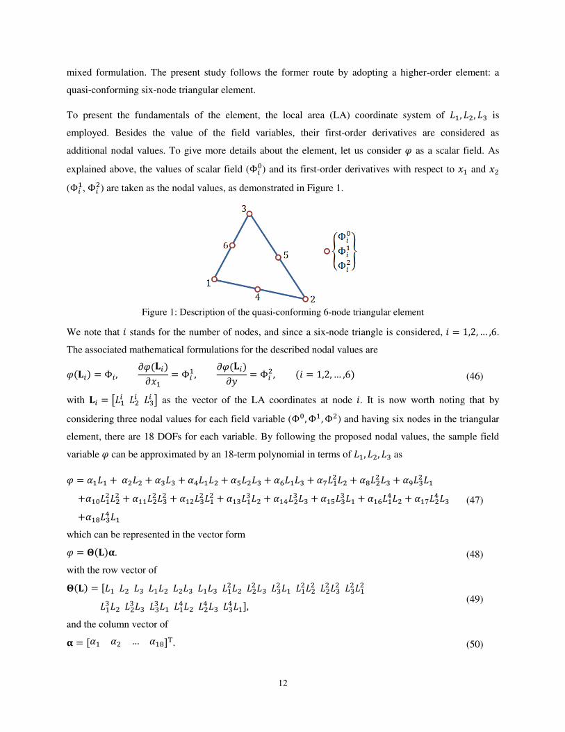
(Φ𝑖1, Φ𝑖2) are taken as the nodal values, as demonstrated in Figure 1.

Figure 1: Description of the quasi-conforming 6-node triangular element

We note that 𝑖 stands for the number of nodes, and since a six-node triangle is considered, 𝑖 = 1,2,… ,6.

The associated mathematical formulations for the described nodal values are 𝜑(𝐋𝑖) = Φ𝑖, 𝜕𝜑(𝐋𝑖)𝜕𝑥1 = Φ𝑖1, 𝜕𝜑(𝐋𝑖)𝜕𝑦 = Φ𝑖2, (𝑖 = 1,2,… ,6) (46)

with 𝐋𝑖 = [𝐿1𝑖 𝐿2𝑖 𝐿3𝑖 ] as the vector of the LA coordinates at node 𝑖. It is now worth noting that by

considering three nodal values for each field variable (Φ0, Φ1, Φ2) and having six nodes in the triangular

element, there are 18 DOFs for each variable. By following the proposed nodal values, the sample field

variable 𝜑 can be approximated by an 18-term polynomial in terms of 𝐿1, 𝐿2, 𝐿3 as 𝜑 = 𝛼1𝐿1 + 𝛼2𝐿2 + 𝛼3𝐿3 + 𝛼4𝐿1𝐿2 + 𝛼5𝐿2𝐿3 + 𝛼6𝐿1𝐿3 + 𝛼7𝐿12𝐿2 + 𝛼8𝐿22𝐿3 + 𝛼9𝐿32𝐿1 +𝛼10𝐿12𝐿22 + 𝛼11𝐿22𝐿32 + 𝛼12𝐿32𝐿12 + 𝛼13𝐿13𝐿2 + 𝛼14𝐿23𝐿3 + 𝛼15𝐿33𝐿1 + 𝛼16𝐿14𝐿2 + 𝛼17𝐿24𝐿3 +𝛼18𝐿34𝐿1

(47)

which can be represented in the vector form 𝜑 = 𝚯(𝐋)𝛂. (48)

with the row vector of 𝚯(𝐋) = [𝐿1 𝐿2 𝐿3 𝐿1𝐿2 𝐿2𝐿3 𝐿1𝐿3 𝐿12𝐿2 𝐿22𝐿3 𝐿32𝐿1 𝐿12𝐿22 𝐿22𝐿32 𝐿32𝐿12 𝐿13𝐿2 𝐿23𝐿3 𝐿33𝐿1 𝐿14𝐿2 𝐿24𝐿3 𝐿34𝐿1], (49)

and the column vector of 𝛂 = [𝛼1 𝛼2 … 𝛼18]T. (50)

13

Since the problem was formulated within the FSDPT with five field variables, i.e., three displacements

(𝑢1, 𝑢2, 𝑢3) and two rotations (𝜓1, 𝜓2), the proposed element has a total of 90 DOFs. Accordingly, the

approximation of Eq. (47) or (48) can be substituted into nodal values conditions of Eq. (46) which leads

to the following relation 𝚽 = 𝚼𝛂, (51)

with 𝚽 = [Φ10 Φ11 Φ12 Φ20 Φ21 Φ22 … Φ60 Φ61 Φ62]T, (52)

𝚼 = [𝚲(𝐋1)𝚲(𝐋2)⋮𝚲(𝐋6)]18×18 , 𝚲(𝐋𝑖) = [ 𝚯(𝐋𝑖)𝜕𝚯(𝐋𝒊)𝜕𝑥1𝜕𝚯(𝐋𝒊)𝜕𝑥2 ]

3×18

. (53)

By using Eq. (51), the column vector 𝛂 can be determined as 𝛂 = 𝚼−𝟏𝚽, and then by following Eq. (48),

the approximation of the sample field variable is obtained as follows: 𝜙 = 𝚯(𝐋)𝚼−𝟏𝚽 = 𝐍𝚽, (54)

where 𝐍 = [𝒩1 𝒩2 … 𝒩18] = 𝚯(𝐋)𝚼−1 introduces the vector of approximate functions which can

be used in Eq. (31) for the approximation functions. The Gauss quadrature can be applied to finally

calculate the stiffness and mass matrices along with the force vector given in Eqs. (40)–(43).

7. Numerical results

The nonlinear shear deformation SG plate model, discretized by the quasi-conforming higher-order

triangular finite element, will be next applied for studying the microarchitecture-dependent free and

forced vibration of cellular plate structures. By employing the SG plate model, the mechanical behavior

of three-dimensional cellular structures with prismatic lattice microarchitectures can be modeled by a

two-dimensional model significantly reducing the computational cost of the numerical structural analysis.

An example of the cellular plates with an equitriangular lattice architecture is shown in Figure 2 and

geometrical parameters are given in Table 1. The SG plate model with the constitutive parameters (as

presented in the material matrices 𝓒, 𝓓1, 𝓓2, 𝓓3, 𝓓4 in Eqs. (20)–(22) and further in (24)) can be

determined by using a homogenization technique in which the deformations of the 2D SG plate model are

compared to the reference full-field model of the classical three-dimensional continuum mechanics. For

the specific equitriangular lattice architecture considered in the present work, Kakalo and Niiranen [48]

have determined the classical and SG material parameters for a reduced SG plate theory, augmented by

Torabi and Niiranen [49]. The nonzero constitutive parameters are given in Tables 2 and 3. Since the

cellular plate is assumed to be made of stainless steel, the mass density is 𝜌 = 7800 (kg/m3), and by

14

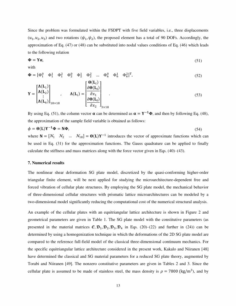
considering the geometrical parameters of the unit cell (see Figure 2b), the value of the factor used in Eq.

(27) is 𝜚 = 0.3.

Figure 2: (a) The schematics of a cellular plate with a triangularly prismatic core and (b) the related plane

geometry of a unit cell

Table 1: The geometries of the unit cell demonstrated in Figure 2b 𝑎1(mm) 𝑎3(mm) 𝑎4(mm) 𝛼° 5 8.66 0.5 60

Table 2: Classical overall constitutive parameters (GPa) for the proposed equitriangular lattice architecture [48] 𝒞11 𝒞12 𝒞22 𝒞44 𝒞55 𝒞66

26.27 6.57 64.96 14.43 9.76 14.43

Table 3: Non-classical SG constitutive parameters (kN) [48,49] 𝒹111 = 𝒹222 = 𝒹113 63.96 𝒹121 = 𝒹122 = 𝒹133 17.59 𝒹221 = 𝒹112 = 𝒹333 50.30 𝒹331 = 𝒹332 = 𝒹114 17.78 𝒹223 = 𝒹334 12.02 𝒹443 = 𝒹224 17.78

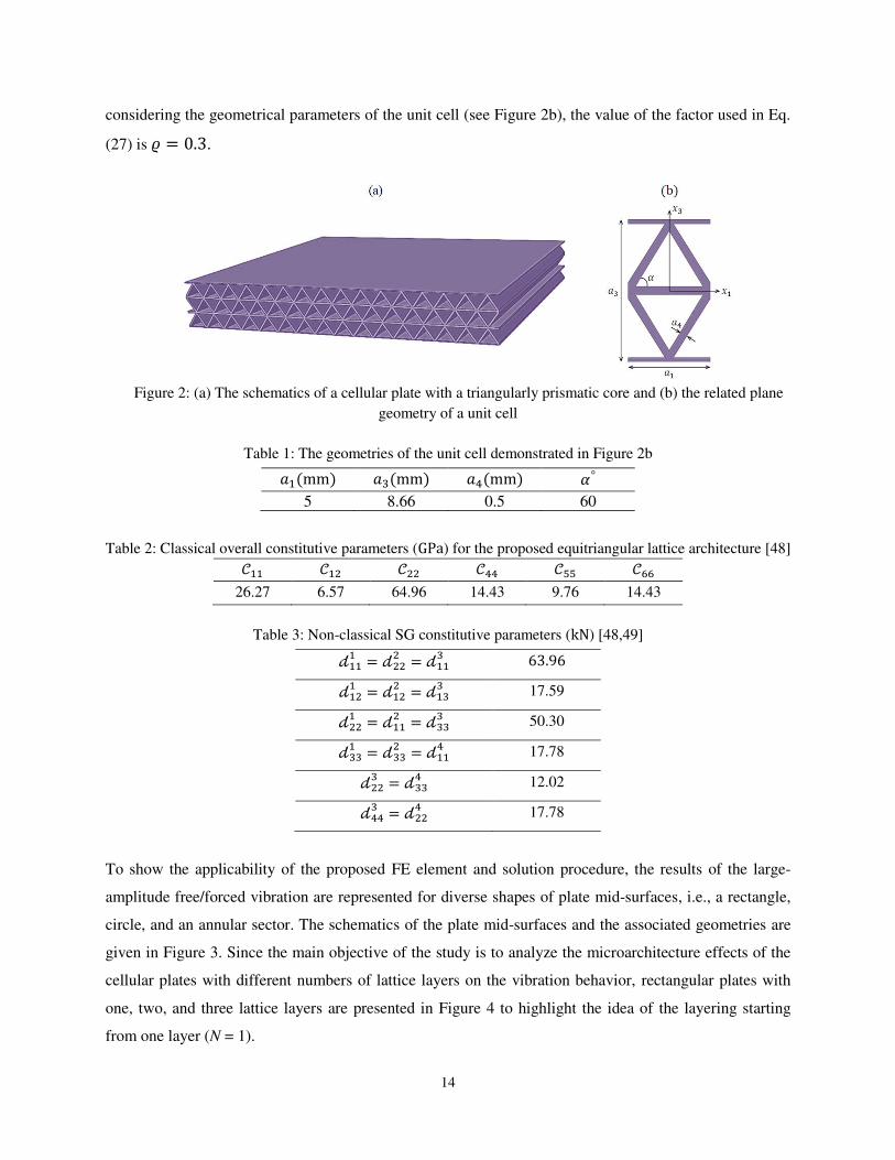
To show the applicability of the proposed FE element and solution procedure, the results of the large-

amplitude free/forced vibration are represented for diverse shapes of plate mid-surfaces, i.e., a rectangle,

circle, and an annular sector. The schematics of the plate mid-surfaces and the associated geometries are

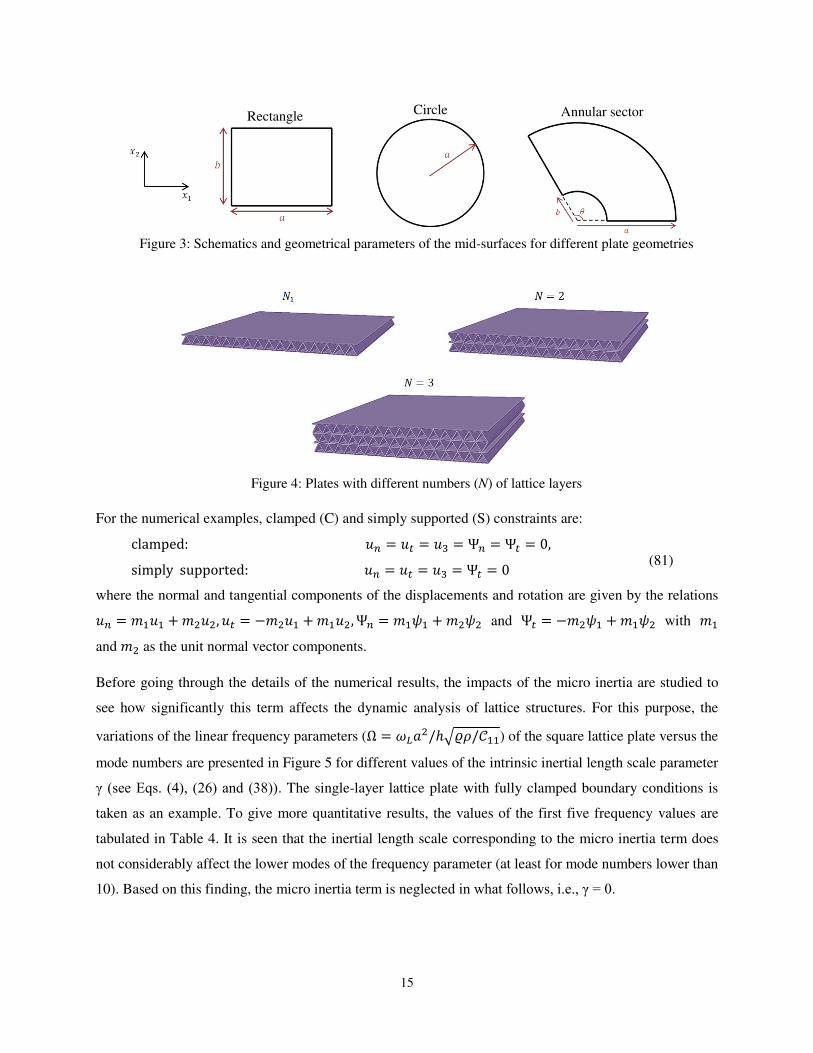
given in Figure 3. Since the main objective of the study is to analyze the microarchitecture effects of the

cellular plates with different numbers of lattice layers on the vibration behavior, rectangular plates with

one, two, and three lattice layers are presented in Figure 4 to highlight the idea of the layering starting

from one layer (N = 1).

15

Rectangle

Circle

Annular sector

Figure 3: Schematics and geometrical parameters of the mid-surfaces for different plate geometries

Figure 4: Plates with different numbers (N) of lattice layers

For the numerical examples, clamped (C) and simply supported (S) constraints are: clamped: 𝑢𝑛 = 𝑢𝑡 = 𝑢3 = Ψ𝑛 = Ψ𝑡 = 0, simply supported: 𝑢𝑛 = 𝑢𝑡 = 𝑢3 = Ψ𝑡 = 0 (81)

where the normal and tangential components of the displacements and rotation are given by the relations 𝑢𝑛 = 𝑚1𝑢1 +𝑚2𝑢2, 𝑢𝑡 = −𝑚2𝑢1 +𝑚1𝑢2, Ψ𝑛 = 𝑚1𝜓1 +𝑚2𝜓2 and Ψ𝑡 = −𝑚2𝜓1 +𝑚1𝜓2 with 𝑚1

and 𝑚2 as the unit normal vector components.

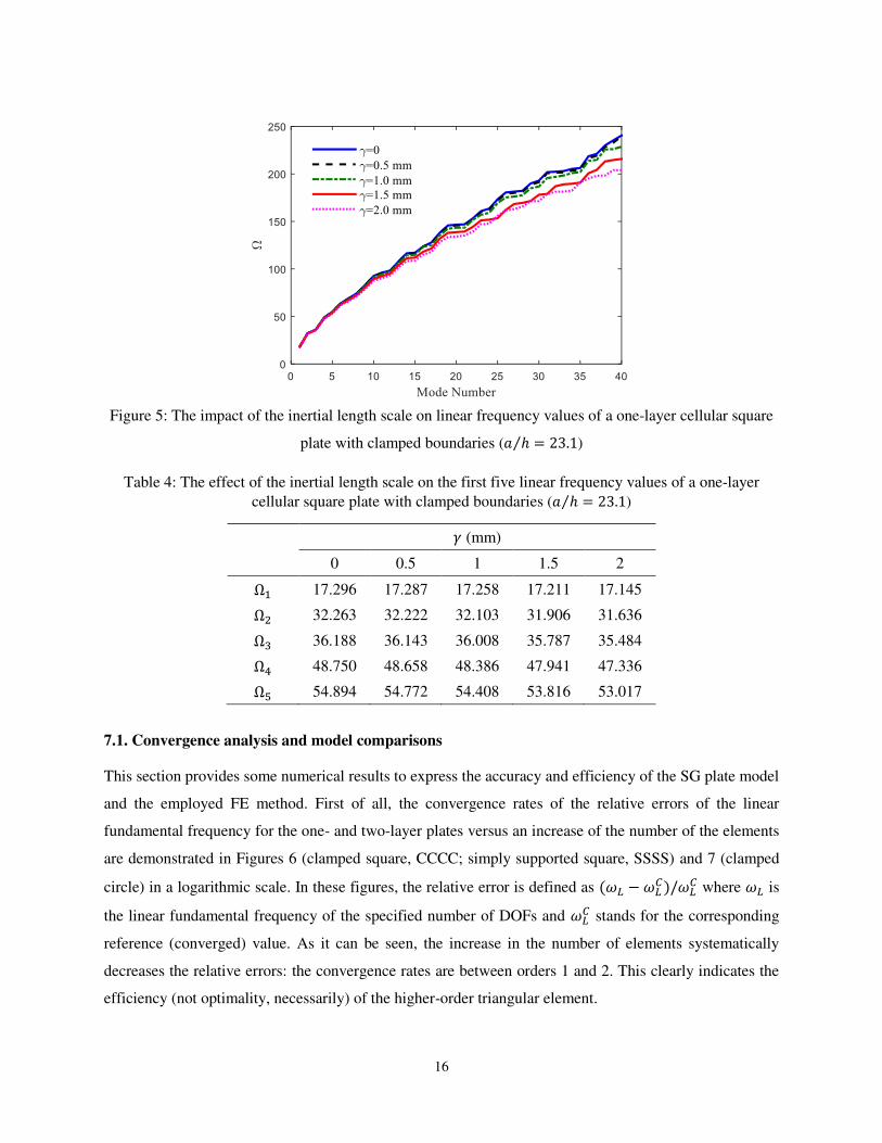
Before going through the details of the numerical results, the impacts of the micro inertia are studied to

see how significantly this term affects the dynamic analysis of lattice structures. For this purpose, the

variations of the linear frequency parameters (Ω = 𝜔𝐿𝑎2/ℎ√𝜚𝜌/𝒞11) of the square lattice plate versus the

mode numbers are presented in Figure 5 for different values of the intrinsic inertial length scale parameter

γ (see Eqs. (4), (26) and (38)). The single-layer lattice plate with fully clamped boundary conditions is

taken as an example. To give more quantitative results, the values of the first five frequency values are

tabulated in Table 4. It is seen that the inertial length scale corresponding to the micro inertia term does

not considerably affect the lower modes of the frequency parameter (at least for mode numbers lower than

10). Based on this finding, the micro inertia term is neglected in what follows, i.e., γ = 0.

16

Figure 5: The impact of the inertial length scale on linear frequency values of a one-layer cellular square

plate with clamped boundaries (𝑎 ℎ⁄ = 23.1)

Table 4: The effect of the inertial length scale on the first five linear frequency values of a one-layer

cellular square plate with clamped boundaries (𝑎 ℎ⁄ = 23.1)

𝛾 (mm)

0 0.5 1 1.5 2 Ω1 17.296 17.287 17.258 17.211 17.145 Ω2 32.263 32.222 32.103 31.906 31.636 Ω3 36.188 36.143 36.008 35.787 35.484 Ω4 48.750 48.658 48.386 47.941 47.336 Ω5 54.894 54.772 54.408 53.816 53.017

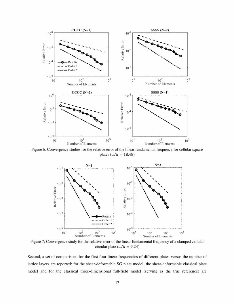
7.1. Convergence analysis and model comparisons

This section provides some numerical results to express the accuracy and efficiency of the SG plate model

and the employed FE method. First of all, the convergence rates of the relative errors of the linear

fundamental frequency for the one- and two-layer plates versus an increase of the number of the elements

are demonstrated in Figures 6 (clamped square, CCCC; simply supported square, SSSS) and 7 (clamped

circle) in a logarithmic scale. In these figures, the relative error is defined as (𝜔𝐿 −𝜔𝐿𝐶)/𝜔𝐿𝐶 where 𝜔𝐿 is

the linear fundamental frequency of the specified number of DOFs and 𝜔𝐿𝐶 stands for the corresponding

reference (converged) value. As it can be seen, the increase in the number of elements systematically

decreases the relative errors: the convergence rates are between orders 1 and 2. This clearly indicates the

efficiency (not optimality, necessarily) of the higher-order triangular element.

17

Figure 6: Convergence studies for the relative error of the linear fundamental frequency for cellular square

plates (𝑎 ℎ⁄ = 18.48)

Figure 7: Convergence study for the relative error of the linear fundamental frequency of a clamped cellular

circular plate (𝑎 ℎ⁄ = 9.24)

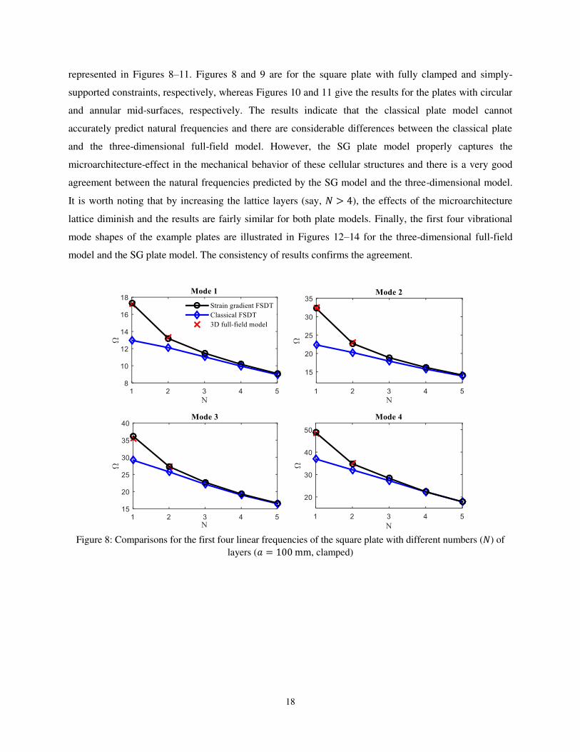
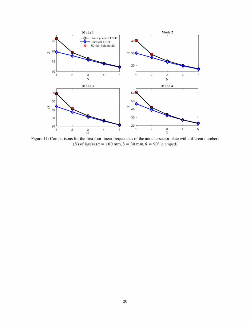
Second, a set of comparisons for the first four linear frequencies of different plates versus the number of

lattice layers are reported; for the shear-deformable SG plate model, the shear-deformable classical plate

model and for the classical three-dimensional full-field model (serving as the true reference) are

18

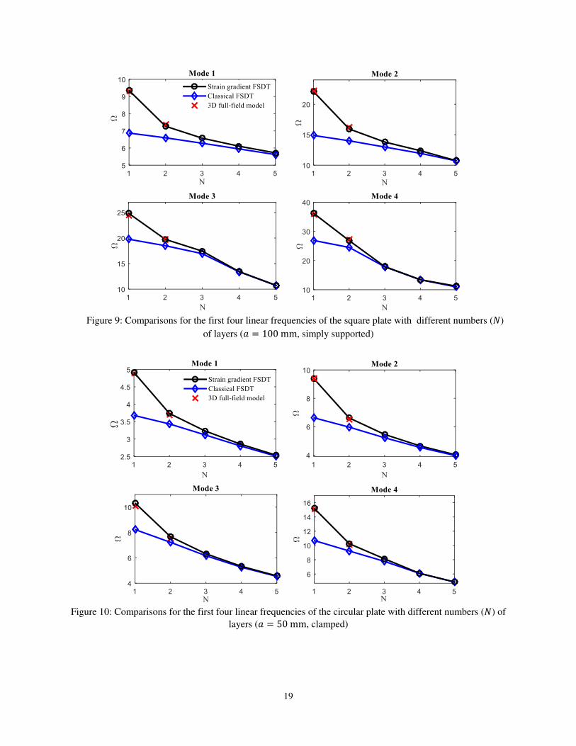
represented in Figures 8–11. Figures 8 and 9 are for the square plate with fully clamped and simply-

supported constraints, respectively, whereas Figures 10 and 11 give the results for the plates with circular

and annular mid-surfaces, respectively. The results indicate that the classical plate model cannot

accurately predict natural frequencies and there are considerable differences between the classical plate

and the three-dimensional full-field model. However, the SG plate model properly captures the

microarchitecture-effect in the mechanical behavior of these cellular structures and there is a very good

agreement between the natural frequencies predicted by the SG model and the three-dimensional model.

It is worth noting that by increasing the lattice layers (say, 𝑁 > 4), the effects of the microarchitecture

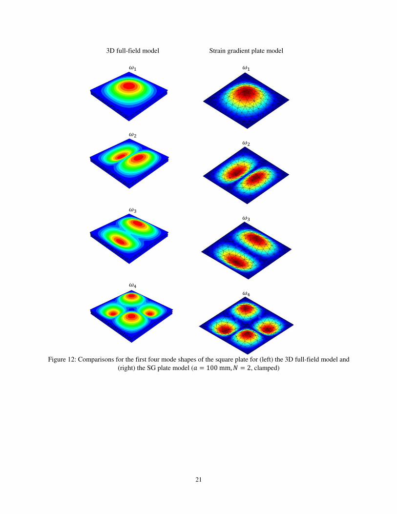
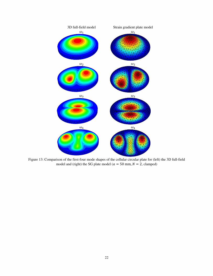
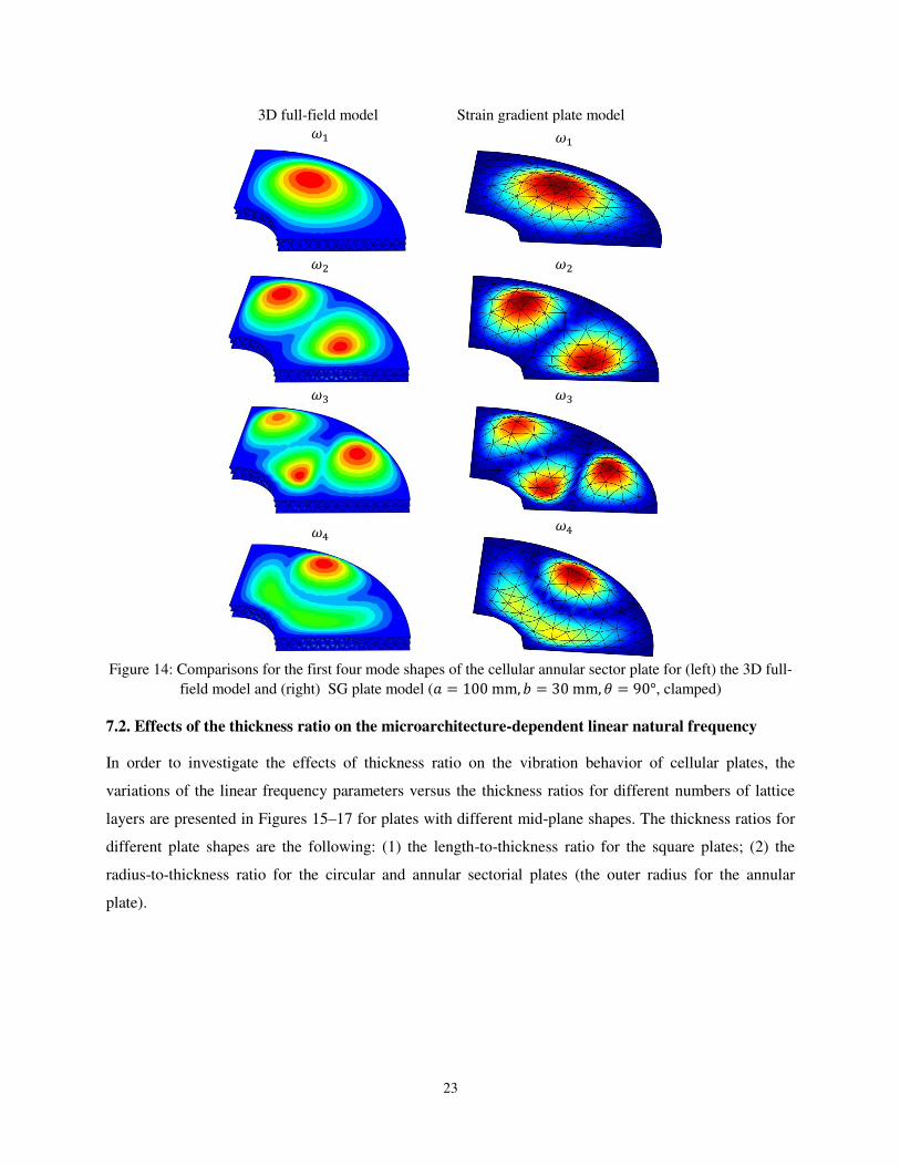
lattice diminish and the results are fairly similar for both plate models. Finally, the first four vibrational

mode shapes of the example plates are illustrated in Figures 12–14 for the three-dimensional full-field

model and the SG plate model. The consistency of results confirms the agreement.

Figure 8: Comparisons for the first four linear frequencies of the square plate with different numbers (𝑁) of

layers (𝑎 = 100 mm, clamped)

19

Figure 9: Comparisons for the first four linear frequencies of the square plate with different numbers (𝑁)

of layers (𝑎 = 100 mm, simply supported)

Figure 10: Comparisons for the first four linear frequencies of the circular plate with different numbers (𝑁) of

layers (𝑎 = 50 mm, clamped)

20

Figure 11: Comparisons for the first four linear frequencies of the annular sector plate with different numbers

(𝑁) of layers (𝑎 = 100 mm, 𝑏 = 30 mm,𝜃 = 90°, clamped)

21

3D full-field model Strain gradient plate model

𝜔1

𝜔1

𝜔2

𝜔2

𝜔3

𝜔3

𝜔4

𝜔4

Figure 12: Comparisons for the first four mode shapes of the square plate for (left) the 3D full-field model and

(right) the SG plate model (𝑎 = 100 mm,𝑁 = 2, clamped)

22

3D full-field model Strain gradient plate model 𝜔1

𝜔1

𝜔2

𝜔2

𝜔3

𝜔3

𝜔4

𝜔4

Figure 13: Comparison of the first-four mode shapes of the cellular circular plate for (left) the 3D full-field

model and (right) the SG plate model (𝑎 = 50 mm,𝑁 = 2, clamped)

23

3D full-field model Strain gradient plate model 𝜔1

𝜔1

𝜔2

𝜔2

𝜔3

𝜔3

𝜔4

𝜔4

Figure 14: Comparisons for the first four mode shapes of the cellular annular sector plate for (left) the 3D full-

field model and (right) SG plate model (𝑎 = 100 mm,𝑏 = 30 mm, 𝜃 = 90°, clamped)

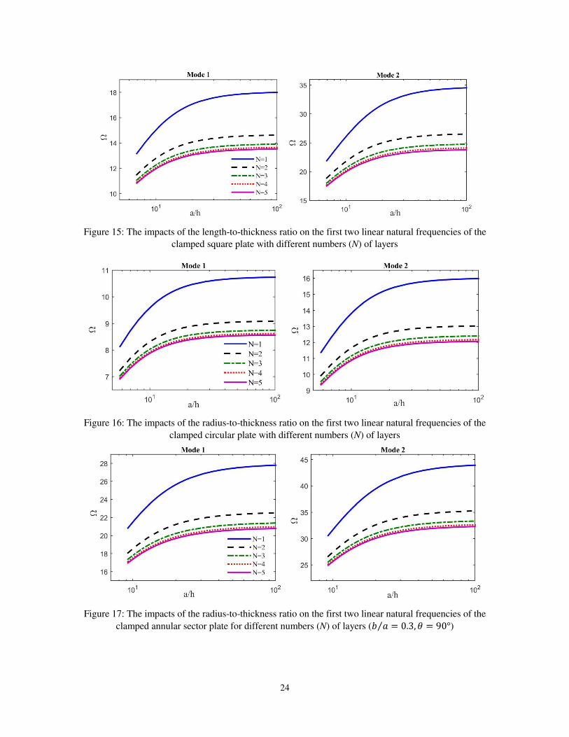
7.2. Effects of the thickness ratio on the microarchitecture-dependent linear natural frequency

In order to investigate the effects of thickness ratio on the vibration behavior of cellular plates, the

variations of the linear frequency parameters versus the thickness ratios for different numbers of lattice

layers are presented in Figures 15–17 for plates with different mid-plane shapes. The thickness ratios for

different plate shapes are the following: (1) the length-to-thickness ratio for the square plates; (2) the

radius-to-thickness ratio for the circular and annular sectorial plates (the outer radius for the annular

plate).

24

Figure 15: The impacts of the length-to-thickness ratio on the first two linear natural frequencies of the

clamped square plate with different numbers (N) of layers

Figure 16: The impacts of the radius-to-thickness ratio on the first two linear natural frequencies of the

clamped circular plate with different numbers (N) of layers

Figure 17: The impacts of the radius-to-thickness ratio on the first two linear natural frequencies of the

clamped annular sector plate for different numbers (N) of layers (𝑏 𝑎⁄ = 0.3, 𝜃 = 90°)

25

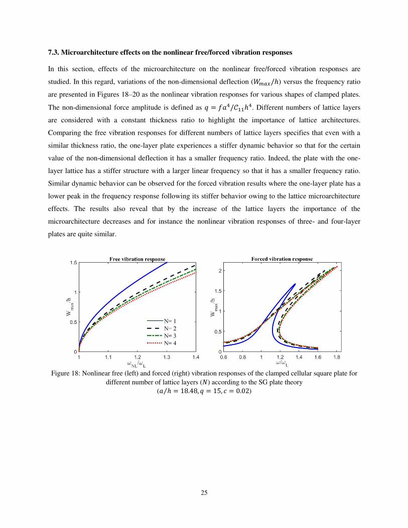
7.3. Microarchitecture effects on the nonlinear free/forced vibration responses

In this section, effects of the microarchitecture on the nonlinear free/forced vibration responses are

studied. In this regard, variations of the non-dimensional deflection (𝑊𝑚𝑎𝑥/ℎ) versus the frequency ratio

are presented in Figures 18–20 as the nonlinear vibration responses for various shapes of clamped plates.

The non-dimensional force amplitude is defined as 𝑞 = 𝑓𝑎4/𝒞11ℎ4. Different numbers of lattice layers

are considered with a constant thickness ratio to highlight the importance of lattice architectures.

Comparing the free vibration responses for different numbers of lattice layers specifies that even with a

similar thickness ratio, the one-layer plate experiences a stiffer dynamic behavior so that for the certain

value of the non-dimensional deflection it has a smaller frequency ratio. Indeed, the plate with the one-

layer lattice has a stiffer structure with a larger linear frequency so that it has a smaller frequency ratio.

Similar dynamic behavior can be observed for the forced vibration results where the one-layer plate has a

lower peak in the frequency response following its stiffer behavior owing to the lattice microarchitecture

effects. The results also reveal that by the increase of the lattice layers the importance of the

microarchitecture decreases and for instance the nonlinear vibration responses of three- and four-layer

plates are quite similar.

Figure 18: Nonlinear free (left) and forced (right) vibration responses of the clamped cellular square plate for

different number of lattice layers (𝑁) according to the SG plate theory

(𝑎 ℎ⁄ = 18.48, 𝑞 = 15, 𝑐 = 0.02)

26

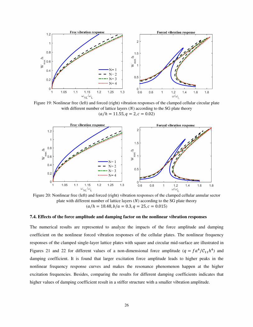
Figure 19: Nonlinear free (left) and forced (right) vibration responses of the clamped cellular circular plate

with different number of lattice layers (𝑁) according to the SG plate theory

(𝑎 ℎ⁄ = 11.55, 𝑞 = 2, 𝑐 = 0.02)

Figure 20: Nonlinear free (left) and forced (right) vibration responses of the clamped cellular annular sector

plate with different number of lattice layers (𝑁) according to the SG plate theory

(𝑎 ℎ⁄ = 18.48, 𝑏/𝑎 = 0.3, 𝑞 = 25, 𝑐 = 0.015)

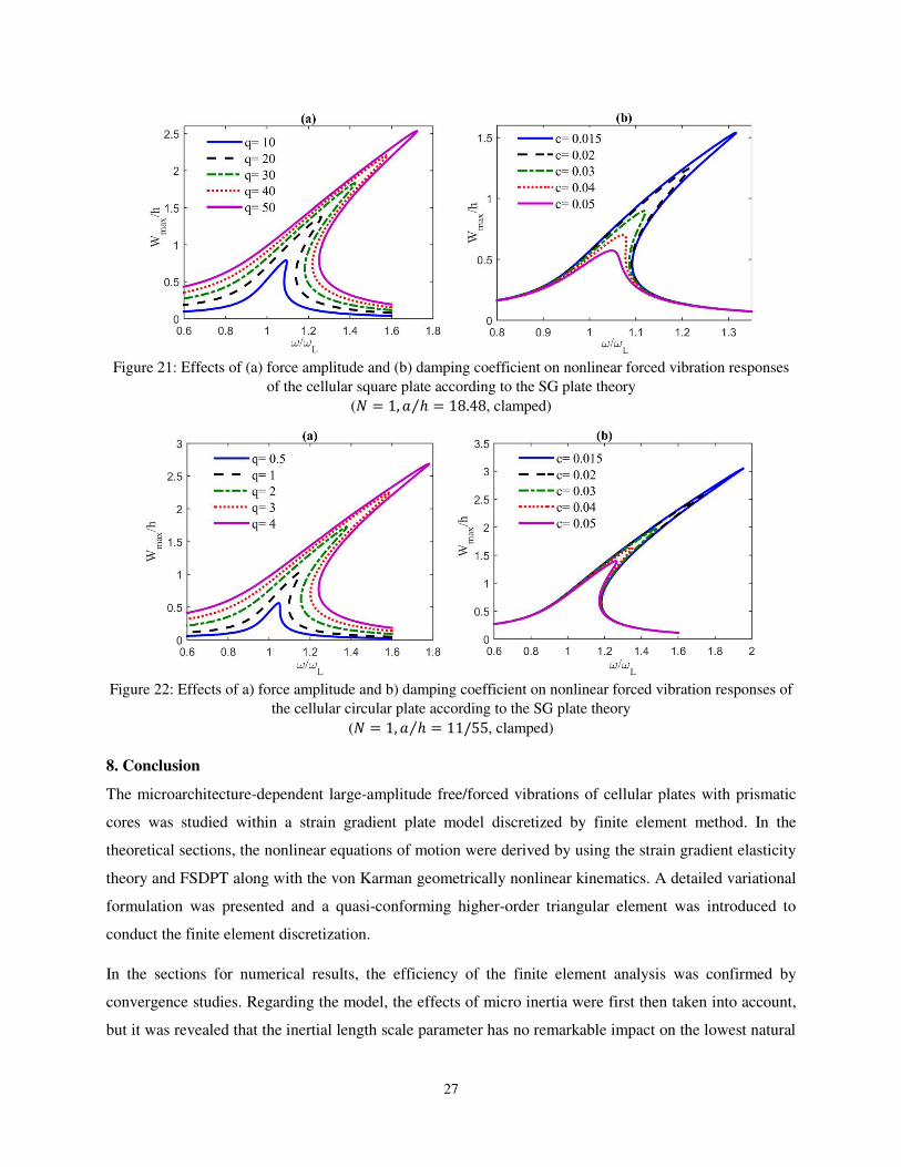
7.4. Effects of the force amplitude and damping factor on the nonlinear vibration responses

The numerical results are represented to analyze the impacts of the force amplitude and damping

coefficient on the nonlinear forced vibration responses of the cellular plates. The nonlinear frequency

responses of the clamped single-layer lattice plates with square and circular mid-surface are illustrated in

Figures 21 and 22 for different values of a non-dimensional force amplitude (𝑞 = 𝑓𝑎4/𝒞11ℎ4) and

damping coefficient. It is found that larger excitation force amplitude leads to higher peaks in the

nonlinear frequency response curves and makes the resonance phenomenon happen at the higher

excitation frequencies. Besides, comparing the results for different damping coefficients indicates that

higher values of damping coefficient result in a stiffer structure with a smaller vibration amplitude.

27

Figure 21: Effects of (a) force amplitude and (b) damping coefficient on nonlinear forced vibration responses

of the cellular square plate according to the SG plate theory

(𝑁 = 1, 𝑎 ℎ⁄ = 18.48, clamped)

Figure 22: Effects of a) force amplitude and b) damping coefficient on nonlinear forced vibration responses of

the cellular circular plate according to the SG plate theory

(𝑁 = 1, 𝑎 ℎ⁄ = 11/55, clamped)

8. Conclusion

The microarchitecture-dependent large-amplitude free/forced vibrations of cellular plates with prismatic

cores was studied within a strain gradient plate model discretized by finite element method. In the

theoretical sections, the nonlinear equations of motion were derived by using the strain gradient elasticity

theory and FSDPT along with the von Karman geometrically nonlinear kinematics. A detailed variational

formulation was presented and a quasi-conforming higher-order triangular element was introduced to

conduct the finite element discretization.

In the sections for numerical results, the efficiency of the finite element analysis was confirmed by

convergence studies. Regarding the model, the effects of micro inertia were first then taken into account,

but it was revealed that the inertial length scale parameter has no remarkable impact on the lowest natural

28

frequencies investigated in the rest of the examples. For a wide range of examples of cellular plates with

different shapes of mid-surface, the response of the plate model was compared to the response of the

corresponding three-dimensional full-field model used as a reference, to address the accuracy of the

proposed two-dimensional model. The results indicated that in the case of constant thickness ratio, the

one-layer lattice plate has the stiffest mechanical behavior with higher natural frequencies due to the

microarchitecture effects. It is also observed that for thin cellular plates the lattice microarchitecture has a

more significant stiffening effect than for thick plates. Besides, it is found that due to the higher impact

of the lattice microarchitecture, the one-layer plate has a lower peak of the forced vibration response.

Comparing the results for plates with different numbers of lattice layers revealed that by the increase of

the number of layers the importance of the lattice microarchitecture diminishes and the dynamic behavior

can be captured by the classical shear-deformable plate theory. All in all, the results provided on the

linear and nonlinear vibration of cellular plates with equitriangular lattice core, along with our previously

published results for plate bending statics [48,49] – to be extended towards shell structures – provide a

comprehensive and reliable basis and efficient simulation tools for the structural design and engineering

of microarchitectural plate structures.

Data Availability Statement: The datasets generated during and/or analyzed during the current study are

available from the corresponding author on reasonable request.

Conflict of interest: The authors declare that they have no conflict of interest.

Funding: No funding was received for conducting this study.

References

1. Schaedler, T. A., & Carter, W. B. (2016). Architected cellular materials. Annual Review of Materials

Research, 46, 187-210, https://doi.org/10.1146/annurev-matsci-070115-031624.

2. Eringen, A. C. (1966). Linear theory of micropolar elasticity. Journal of Mathematics and Mechanics,

15, 909-923, http://www.jstor.org/stable/24901442

3. Mindlin, R. D. (1964). Micro-structure in linear elasticity. Archive for Rational Mechanics and

Analysis, 16(1), 51-78.

4. Mindlin, R. D. (1965). Second gradient of strain and surface-tension in linear elasticity. International

Journal of Solids and Structures, 1(4), 417-438, https://doi.org/10.1016/0020-7683(65)90006-5.

5. Eringen, A. C. (1972). Linear theory of nonlocal elasticity and dispersion of plane

waves. International Journal of Engineering Science, 10(5), 425-435, https://doi.org/10.1016/0020-

7225(72)90050-X.

29

6. Lam, D. C., Yang, F., Chong, A. C. M., Wang, J., & Tong, P. (2003). Experiments and theory in

strain gradient elasticity. Journal of the Mechanics and Physics of Solids, 51(8), 1477-1508,

https://doi.org/10.1016/S0022-5096(03)00053-X.

7. Haque, M. A., & Saif, M. T. A. (2003). Strain gradient effect in nanoscale thin films. Acta Materialia,

51(11), 3053-3061, https://doi.org/10.1016/S1359-6454(03)00116-2.

8. Thai, H. T., Vo, T. P., Nguyen, T. K., & Kim, S. E. (2017). A review of continuum mechanics models

for size-dependent analysis of beams and plates. Composite Structures, 177, 196-219,

https://doi.org/10.1016/j.compstruct.2017.06.040.

9. Andreaus, U., Dell’Isola, F., Giorgio, I., Placidi, L., Lekszycki, T., & Rizzi, N. L. (2016). Numerical

simulations of classical problems in two-dimensional (non) linear second gradient

elasticity. International Journal of Engineering Science, 108, 34-50,

https://doi.org/10.1016/j.ijengsci.2016.08.003.

10. Ansari, R., & Torabi, J. (2016). Numerical study on the free vibration of carbon nanocones resting on

elastic foundation using nonlocal shell model. Applied Physics A, 122(12), 1-13,

https://doi.org/10.1007/s00339-016-0602-x.

11. Awrejcewicz, J., Kudra, G., & Mazur, O. (2021). Double mode model of size-dependent chaotic

vibrations of nanoplates based on the nonlocal elasticity theory. Nonlinear Dynamics,

https://doi.org/10.1007/s11071-021-06224-6.

12. Niiranen, J., & Niemi, A. H. (2017). Variational formulations and general boundary conditions for

sixth-order boundary value problems of gradient-elastic Kirchhoff plates. European Journal of

Mechanics-A/Solids, 61, 164-179, https://doi.org/10.1016/j.euromechsol.2016.09.001.

13. Khakalo, S., & Niiranen, J. (2017). Gradient-elastic stress analysis near cylindrical holes in a plane

under bi-axial tension fields. International Journal of Solids and Structures, 110, 351-366,

https://doi.org/10.1016/j.ijsolstr.2016.10.025.

14. Ansari, R., Torabi, J., & Norouzzadeh, A. (2020). An integral nonlocal model for the free vibration

analysis of Mindlin nanoplates using the VDQ method. The European Physical Journal Plus, 135(2),

206, https://doi.org/10.1140/epjp/s13360-019-00018-x.

15. Ghayesh, M. H., & Farokhi, H. (2016). Parametric instability of microbeams in supercritical regime.

Nonlinear Dynamics, 83(3), 1171-1183, https://doi.org/10.1007/s11071-015-2395-4.

16. Ansari, R., Oskouie, M. F., & Rouhi, H. (2017). Studying linear and nonlinear vibrations of fractional

viscoelastic Timoshenko micro-/nano-beams using the strain gradient theory. Nonlinear Dynamics,

87(1), 695-711, https://doi.org/10.1007/s11071-016-3069-6.

30

17. Rouhi, H., Ebrahimi, F., Ansari, R., & Torabi, J. (2019). Nonlinear free and forced vibration analysis

of Timoshenko nanobeams based on Mindlin's second strain gradient theory. European Journal of

Mechanics-A/Solids, 73, 268-281, https://doi.org/10.1016/j.euromechsol.2018.09.005.

18. Lazopoulos, K. A. (2009). On bending of strain gradient elastic micro-plates. Mechanics Research

Communications, 36(7), 777-783, https://doi.org/10.1016/j.mechrescom.2009.05.005.

19. Wang, B., Zhou, S., Zhao, J., & Chen, X. (2011). A size-dependent Kirchhoff micro-plate model

based on strain gradient elasticity theory. European Journal of Mechanics-A/Solids, 30(4), 517-524,

https://doi.org/10.1016/j.euromechsol.2011.04.00.

20. Ramezani, S. (2013). Nonlinear vibration analysis of micro-plates based on strain gradient elasticity

theory. Nonlinear Dynamics, 73(3), 1399-1421, https://doi.org/10.1007/s11071-013-0872-1.

21. Soni, S., Jain, N. K., & Joshi, P. V. (2019). Vibration and deflection analysis of thin cracked and

submerged orthotropic plate under thermal environment using strain gradient theory. Nonlinear

Dynamics, 96(2), 1575-1604, https://doi.org/10.1007/s11071-019-04872-3.

22. Gholami, R., & Ansari, R. (2016). A most general strain gradient plate formulation for size-dependent

geometrically nonlinear free vibration analysis of functionally graded shear deformable rectangular

microplates. Nonlinear Dynamics, 84(4), 2403-2422, https://doi.org/10.1007/s11071-016-2653-0.

23. Balobanov, V., Kiendl, J., Khakalo, S., & Niiranen, J. (2019). Kirchhoff–Love shells within strain

gradient elasticity: weak and strong formulations and an H3-conforming isogeometric

implementation. Computer Methods in Applied Mechanics and Engineering, 344, 837-857,

https://doi.org/10.1016/j.cma.2018.10.006.

24. Zervos, A., Papanicolopulos, S. A., & Vardoulakis, I. (2009). Two finite-element discretizations for

gradient elasticity. Journal of engineering mechanics, 135(3), 203-213,

https://doi.org/10.1061/(ASCE)0733-9399(2009)135:3(203).

25. Askes, H., Morata, I., & Aifantis, E. C. (2008). Finite element analysis with staggered gradient

elasticity. Computers & Structures, 86(11-12), 1266-1279,

https://doi.org/10.1016/j.compstruc.2007.11.002.

26. Torabi, J., Ansari, R., & Darvizeh, M. (2018). A C1 continuous hexahedral element for nonlinear

vibration analysis of nano-plates with circular cutout based on 3D strain gradient theory. Composite

Structures, 205, 69-85, https://doi.org/10.1016/j.compstruct.2018.08.070.

27. Bacciocchi, M., Fantuzzi, N., & Ferreira, A. J. M. (2020). Conforming and nonconforming laminated

finite element Kirchhoff nanoplates in bending using strain gradient theory. Computers & Structures,

239, 106322, https://doi.org/10.1016/j.compstruc.2020.106322.

31

28. Ansari, R., Shojaei, M. F., Mohammadi, V., Bazdid-Vahdati, M., & Rouhi, H. (2015). Triangular

Mindlin microplate element. Computer Methods in Applied Mechanics and Engineering, 295, 56-76,

https://doi.org/10.1016/j.cma.2015.06.004.

29. Torabi, J., Niiranen, J., & Ansari, R. (2021). Nonlinear finite element analysis within strain gradient

elasticity: Reissner-Mindlin plate theory versus three-dimensional theory. European Journal of

Mechanics-A/Solids, 87, 104221, https://doi.org/10.1016/j.euromechsol.2021.104221.

30. Fischer, P., Klassen, M., Mergheim, J., Steinmann, P., & Müller, R. (2011). Isogeometric analysis of

2D gradient elasticity. Computational Mechanics, 47(3), 325-334, https://doi.org/10.1007/s00466-

010-0543-8.

31. Niiranen, J., Khakalo, S., Balobanov, V., & Niemi, A. H. (2016). Variational formulation and

isogeometric analysis for fourth-order boundary value problems of gradient-elastic bar and plane

strain/stress problems. Computer Methods in Applied Mechanics and Engineering, 308, 182-211,

https://doi.org/10.1016/j.cma.2016.05.008.

32. Thai, S., Thai, H. T., Vo, T. P., & Nguyen-Xuan, H. (2017). Nonlinear static and transient

isogeometric analysis of functionally graded microplates based on the modified strain gradient

theory. Engineering Structures, 153, 598-612, https://doi.org/10.1016/j.engstruct.2017.10.002.

33. Niiranen, J., Balobanov, V., Kiendl, J., & Hosseini, S. B. (2019). Variational formulations, model

comparisons and numerical methods for Euler–Bernoulli micro-and nano-beam models. Mathematics

and Mechanics of Solids, 24(1), 312-335, https://doi.org/10.1177/1081286517739669.

34. dell'Isola, F., & Steigmann, D. J. (Eds.). (2020). Discrete and Continuum Models for Complex

Metamaterials. Cambridge University Press.

35. Bacigalupo, A., & Gambarotta, L. (2019). Generalized micropolar continualization of 1D beam

lattices. International Journal of Mechanical Sciences, 155, 554-570,

https://doi.org/10.1016/j.ijmecsci.2019.02.018.

36. Da, D., Yvonnet, J., Xia, L., Le, M. V., & Li, G. (2018). Topology optimization of periodic lattice

structures taking into account strain gradient. Computers & Structures, 210, 28-40,

https://doi.org/10.1016/j.compstruc.2018.09.003.

37. Polyzos, D., & Fotiadis, D. I. (2012). Derivation of Mindlin’s first and second strain gradient elastic

theory via simple lattice and continuum models. International Journal of Solids and Structures, 49(3-

4), 470-480, https://doi.org/10.1016/j.ijsolstr.2011.10.021.

38. Auffray, N., Bouchet, R., & Brechet, Y. (2010). Strain gradient elastic homogenization of

bidimensional cellular media. International Journal of Solids and Structures, 47(13), 1698-1710,

https://doi.org/10.1016/j.ijsolstr.2010.03.011.

32

39. Yang, H., Timofeev, D., Giorgio, I., & Müller, W. H. (2020). Effective strain gradient continuum

model of metamaterials and size effects analysis. Continuum Mechanics and Thermodynamics, doi:

10.1007/s00161-020-00910-3, https://doi.org/10.1007/s00161-020-00910-3.

40. Tran, L. V., and Niiranen, J. (2020). A geometrically nonlinear Euler–Bernoulli beam model within

strain gradient elasticity with isogeometric analysis and lattice structure applications. Mathematics

and Mechanics of Complex Systems, 8(4), 345–371, doi: 10.2140/memocs.2020.8.345.

41. Rueger, Z., Ha, C. S., & Lakes, R. S. (2019). Cosserat elastic lattices. Meccanica, 54(13), 1983-1999,

https://doi.org/10.1007/s11012-019-00968-7.

42. Karttunen, A. T., Reddy, J. N., & Romanoff, J. (2019). Two-scale micropolar plate model for web-

core sandwich panels. International Journal of Solids and Structures, 170, 82-94,

https://doi.org/10.1016/j.ijsolstr.2019.04.026.

43. Nampally, P., Karttunen, A. T., & Reddy, J. N. (2020). Nonlinear finite element analysis of lattice

core sandwich plates. International Journal of Non-Linear Mechanics, 121, 103423,

https://doi.org/10.1016/j.ijnonlinmec.2020.103423.

44. Rahali, Y., Giorgio, I., Ganghoffer, J. F., & dell'Isola, F. (2015). Homogenization à la Piola produces

second gradient continuum models for linear pantographic lattices. International Journal of

Engineering Science, 97, 148-172, https://doi.org/10.1016/j.ijengsci.2015.10.003.

45. Dell’Isola, F., Seppecher, P., Spagnuolo, M.,... & Hayat, T. (2019). Advances in pantographic

structures: design, manufacturing, models, experiments and image analyses. Continuum Mechanics

and Thermodynamics, 31(4), 1231-1282, https://doi.org/10.1007/s00161-019-00806-x.

46. Khakalo, S., Balobanov, V., & Niiranen, J. (2018). Modelling size-dependent bending, buckling and

vibrations of 2D triangular lattices by strain gradient elasticity models: applications to sandwich

beams and auxetics. International Journal of Engineering Science, 127, 33-52,

https://doi.org/10.1016/j.ijengsci.2018.02.004.

47. Khakalo, S., & Niiranen, J. (2019). Lattice structures as thermoelastic strain gradient metamaterials:

Evidence from full-field simulations and applications to functionally step-wise-graded

beams. Composites Part B: Engineering, 177, 107224,

https://doi.org/10.1016/j.compositesb.2019.107224.

48. Khakalo, S., & Niiranen, J. (2020). Anisotropic strain gradient thermoelasticity for cellular structures:

Plate models, homogenization and isogeometric analysis. Journal of the Mechanics and Physics of

Solids, 134, 103728, https://doi.org/10.1016/j.jmps.2019.103728.

49. Torabi, J., & Niiranen, J. (2021). Microarchitecture-dependent nonlinear bending analysis for cellular

plates with prismatic corrugated cores via an anisotropic strain gradient plate theory of first-order

33

shear deformation. Engineering Structures, 236, 112117,

https://doi.org/10.1016/j.engstruct.2021.112117.

50. Madeo, A., Neff, P., Ghiba, I. D., Placidi, L., & Rosi, G. (2015). Wave propagation in relaxed

micromorphic continua: modeling metamaterials with frequency band-gaps. Continuum Mechanics

and Thermodynamics, 27(4), 551-570, https://doi.org/10.1007/s00161-013-0329-2.

51. Reda, H., Ganghoffer, J. F., & Lakiss, H. (2017). Micropolar dissipative models for the analysis of

2D dispersive waves in periodic lattices. Journal of Sound and Vibration, 392, 325-345,

https://doi.org/10.1016/j.jsv.2016.12.007.

52. Salehian, A., & Inman, D. J. (2010). Micropolar continuous modeling and frequency response

validation of a lattice structure. Journal of Vibration and Acoustics, 132(1), 011010,

https://doi.org/10.1115/1.4000472.

53. Liu, F., Wang, L., Jin, D., Liu, X., & Lu, P. (2020). Equivalent micropolar beam model for spatial

vibration analysis of planar repetitive truss structure with flexible joints. International Journal of

Mechanical Sciences, 165, 105202, https://doi.org/10.1016/j.ijmecsci.2019.105202.

54. Su, W., & Liu, S. (2014). Vibration analysis of periodic cellular solids based on an effective couple-

stress continuum model. International Journal of Solids and Structures, 51(14), 2676-2686,

https://doi.org/10.1016/j.ijsolstr.2014.03.043.

55. Challamel, N., Hache, F., Elishakoff, I., & Wang, C. M. (2016). Buckling and vibrations of

microstructured rectangular plates considering phenomenological and lattice-based nonlocal

continuum models. Composite Structures, 149, 145-156,

https://doi.org/10.1016/j.compstruct.2016.04.007.

56. Hasrati, E., Ansari, R., & Torabi, J. (2018). A novel numerical solution strategy for solving nonlinear

free and forced vibration problems of cylindrical shells. Applied Mathematical Modelling, 53, 653-

672, https://doi.org/10.1016/j.apm.2017.08.027.

57. Ansari, R., Shojaei, M. F., & Gholami, R. (2016). Size-dependent nonlinear mechanical behavior of

third-order shear deformable functionally graded microbeams using the variational differential

quadrature method. Composite Structures, 136, 669-683,

https://doi.org/10.1016/j.compstruct.2015.10.043.