nonlinear fluid-structure interaction problem. part ii
TRANSCRIPT
HAL Id: hal-00603368https://hal-enpc.archives-ouvertes.fr/hal-00603368
Submitted on 24 Jun 2011
HAL is a multi-disciplinary open accessarchive for the deposit and dissemination of sci-entific research documents, whether they are pub-lished or not. The documents may come fromteaching and research institutions in France orabroad, or from public or private research centers.
L’archive ouverte pluridisciplinaire HAL, estdestinée au dépôt et à la diffusion de documentsscientifiques de niveau recherche, publiés ou non,émanant des établissements d’enseignement et derecherche français ou étrangers, des laboratoirespublics ou privés.
Nonlinear fluid-structure interaction problem. Part II:space discretization, implementation aspects, nested
parallelization and application examplesChristophe Kassiotis, Adnan Ibrahimbegovic, Rainer Niekamp, Hermann
Matthies
To cite this version:Christophe Kassiotis, Adnan Ibrahimbegovic, Rainer Niekamp, Hermann Matthies. Nonlinear fluid-structure interaction problem. Part II: space discretization, implementation aspects, nested paral-lelization and application examples. Computational Mechanics, Springer Verlag, 2011, 47, pp.335-357.10.1007/s00466-010-0544-7. hal-00603368
Computational Mechanics manuscript No.
(will be inserted by the editor)
Nonlinear fluid-structure interaction problem. Part II: space
discretization, implementation aspects, nested parallelization
and application examples
Christophe Kassiotis · Adnan Ibrahimbegovic ·Rainer Niekamp · Hermann G. Matthies
the date of receipt and acceptance should be inserted later
Abstract The main focus of the present article is the development of a general solution
framework for coupled and/or interaction multi-physics problems based upon re-using ex-
isting codes into software products. In particular, we discuss how to build this software tool
for the case of fluid-structure interaction problem, from finite element code FEAP for struc-
tural and finite volume code OpenFOAM for fluid mechanics. This is achieved by using the
Component Template Library (CTL) to provide the coupling between the existing codes
into a single software product. The present CTL code-coupling procedure accepts not only
different discretization schemes, but different languages, with the solid component written
in Fortran and fluid component written in C++. Moreover, the resulting CTL-based code also
accepts the nested parallelization. The proposed coupling strategy is detailed for explicit and
implicit fixed-point iteration solver presented in the Part I of this paper, referred to Direct
Force-Motion Transfer/Block-Gauss-Seidel. However, the proposed code-coupling frame-
work can easily accommodate other solution schemes. The selected application examples
are chosen to confirm the capability of the code-coupling strategy to provide a quick de-
velopment of advanced computational tools for demanding practical problems, such as 3D
fluid models with free-surface flows interacting with structures.
Keywords fluid-structure interaction · CTL implementation · finite element · finite volume
C. Kassiotis
Saint-Venant Laboratory for Hydraulics, Universite Paris-Est (Joint Research Unit EDF R&D, CETMEF,
Ecole des Ponts ParisTech), 6 quai Watier, BP 49, 78401 Chatou, France
E-mail: [email protected]
A. Ibrahimbegovic
LMT-Cachan (ENS Cachan/CNRS/UPMC/PRES UniverSud Paris), 61 avenue du President Wilson, F-94230
Cachan, France
E-mail: [email protected]
R. Niekamp · H. G. Matthies
Institut fur Wissenschaftliches Rechnen (TU-Braunschweig), D-38092 Braunschweig
E-mail: [email protected]
2
1 Introduction
The main thrust of this paper is geared towards the quick developments of computational
tools for currently interesting multi-physics problems, pertaining to coupling or interaction
of two or more traditional scientific domains. Of main interest for this work is how to pro-
vide the most efficient development of the corresponding software for this kind of problems,
by coupling the stand alone software products from each traditional domain. The latter are
often programmed by experts of a particular domain, with a strong preference to a partic-
ular discretization technique, programming language, or other special choices that provide
the optimal result. Such an optimal result can in general be produced only by the corre-
sponding domain experts, software designer and programmer, with a deep understanding
of both physical phenomena and of numerical analysis issues pertaining to this particular
domain. Hardly anybody can gain such level of expertise in many different domains. There-
fore, the current trends in engineering developments geared towards multi-physics problems
(e.g. fluid-structure interaction, thermomechanical coupling [48], mechanics and optimiza-
tion [39], mechanics and control [40]) are rather difficult to deal with, not only in terms of
theoretical formulations but also in terms of development of corresponding software tools.
One way to avoid this difficulty, as proposed and discussed in this work, is by coupling of
different software products, each produced by experts for a particular sub-problem.
This flexibility in problem formulation and tools development should not be penalized
with a severe lack of solution efficiency. Namely, we are interested in development of soft-
ware tools for solving the problems relevant to industrial applications, which implies using
fine discretization and mesh with many d-o-f; the examples of this kind are the problems
reaching the half a billion d-o-f from solid mechanics applications to bio-mechanics [1] or
the large CFD computations pertinent to meteorological prediction or climate change [28].
For the lack of efficiency, most symbolic interpreter software products, such as Matlab or
Octave, are not suitable for this class of problems. In fact, in order to ensure the required
level of computational efficiency in the context of fluid-structure interaction [3,5,10,15,17,
18,20,21,22,23,24,26,27,34,36,45,54,51,52,53,58,57,59,65,66,68,72,73,70,74,78,79],
large size problems are often tackled using dedicated software developments [60,72,71,73].
In this work, the large problems from fluid-structure interactionapplications are solved by
using existing fluid and structure solvers, along with the corresponding partitioned strat-
egy. The nested parallel computations, exploiting parallelization for both the fluid flow and
interface interaction, are used to ensure the computational efficiency.
Granted sufficient efficiency, the strategy of re-using the stand-alone software for par-
ticular sub-problems is likely to become the most efficient way in development of software
products for multi-physics applications. Indeed, in order to produce a reliable new software
(and a bug-free code), the testing and validation is often the most time consuming phase that
concerns not only the programmers and code developers but also the end-users. Namely,
only after extensive use of a particular software product (by end-users), can we count with
sufficient reliability of a particular software product. It is tacitly assumed that a reliable soft-
ware product will keep its reliability in a more general framework of multi-physics prob-
lems.
Therefore, the proposed strategy of re-using software products (or components) for solv-
ing multi-physics problems, is currently becoming one of the major trends in scientific com-
puting. The component-coupling framework described in this work, which allows to re-use
existing codes for the fluid-structure interaction, is based upon the middleware CTL (Com-
munication Template Library, see [62,56]) handling communication between components.
The main novelty for CTL implementation presented in this work concerns the use of nested

3
parallelization for fluid-structure interactioncomputations, where the parallel communica-
tion is mastered by the CTL, and the call to a parallel component is transparent for the
client.
The outline of the paper is as follows. In the next section we give a description of the
space discretization methods used for structure and fluid; we combine herein geometrically
nonlinear models for structure discretized by Finite Elements [38] and a free-surface fluid
flow formulation (based upon the Volume-Of-Fluid strategy [7,30,55,75]) discretized by
the Finite Volume [25]. In Section 3 we describe how to provide the compatible space inter-
polations between two different discretizations on fluid-structure interface, and thus enforce
the corresponding interaction. It is also shown how the chosen method to ensure compat-
ibility of fields between the structure and fluid solvers can be implemented as a separate
CTL–component that can be coupled with a number of different codes (see also [46]). The
performance of parallel computations with fluid component and the CTL-based nested par-
allelization of fluid-structure interactionproblems is studied in Section 4. The numerical
simulations with a couple of large three-dimensional numerical examples, including large
number of d-o-f and application to free surface flows, are given in Section 4. The concluding
remarks are stated the last section.
2 Structure and fluid formulations
We start by giving the field discretization details typically used for solids and fluids, which
are important to understand.
2.1 Structure equations of motion
The structure motion is based on the Lagrangian description. Namely, we consider a struc-
ture domain Ωs with imposed displacements u on the Dirichlet boundary ∂Ωs,D and moving
under the loading of traction forces t on the Neumann boundary ∂Ωs,N and a body force
b applied in the whole domain Ωs. This dynamic motion has to be computed in the time
interval [0,T ]. The Cauchy governing equation for the structure describes the momentum
conservation. The strong form of this equation can be written with respect to the deformed
configuration as follows; given u on ∂Ωs,D × [0,T ], t on ∂Ωs,N × [0,T ] and b in Ωs × [0,T ],find: u ∈ Ωs × [0,T ] so that:
∇ · JσF−T
︸ ︷︷ ︸
P
+ρs
(b−∂ 2
t u)= 0 in Ωs × [0,T ] (1)
where ρs denotes the material density of the solid domain, u its displacement field and
∂ 2t u the accelerations. We indicated above that the Cauchy stress tensor σ in the deformed
configuration can be linked to the first Piola-Kirchhoff stress tensor P formulated in the
initial configuration through the gradient F of the deformation and its Jacobian J (see [38]).
To close this Partial Differential Equations system we will link the displacements (or
rather its derivatives) with the stresses through constitutive law. For instance, an elastic ma-
terial model based on St.-Venant-Kirchhoff constitutive equation is assumed that links the
Cauchy stress tensor σ and the Green-Lagrange strain tensor E through:
F−1JσF−T = C : E, E =1
2
(FT F− I
)and F = I+∇u (2)

4
where C denotes the constitutive fourth-order elasticity tensor1. Thus, it is a priori impos-
sible to find directly an exact solution to the problem defined above. The idea is to find
the best approximation of the solution in a finite-dimensional space where the solution can
be found numerically. The FEM approximation [9,80,38] derived from weak forms of the
equilibrium equation (1) and can be written for this problem as given t on ∂Ωs,N × [0,T ] and
b in Ωs × [0,T ], find u ∈ U such that, for all δu ∈ U0:
Gs(u;δu) :=∫
Ωs
ρs∂2t u ·δu+
∫
Ωs
σ : ∇δu−∫
Ωs
b ·δu−∫
∂Ωs
t ·δu
= 0
where U and U0 are functional spaces for the solution and its variation.
The solid domain Ωs is then discretized in a finite number of sub-domains or elements
Th = (κe)e=1,...,nelso that the whole space is covered with the finite elements that do not
intersect. The solution space associated with this approximation solution is restrained to the
space of continuous element-wise polynomial functions, which is denoted:
Uh = U ∩
u ∈ C0 (Ωs)
∣∣∣u|κ ∈ P
p (κ) ,∀κ ∈ Th
(3)
where P p (κ) is the space of polynomials of order p on κ . The same restriction U h0 holds
on the associated vector space. The semi-discretized FE problem is defined as given t on
∂Ωs,N and b in Ωs, find u ∈ U h such that, for all δu ∈ U h0 :
Gs(u;δu) = 0 (4)
This semi-discrete problem can also be written in a matrix notation by using the real valued
vectors u ∈ nd−o− f :
Rs(us;λ ) :=Msus + f ints (us)− fext
s (λ ) = 0 (5)
where M is the mass matrix, f ints with a geometrically nonlinear problem, and fext
s the con-
sistent nodal forces. Here the λ represents the boundary forces computed from the fluid
flow problem and imposed on the fluid-structure interface. Each matrix and vector of this
semi-discrete equation are properly defined by assembling locally computed array in each
element with the polynomial basis Ne of P (κe):
Ms,e =∫
κe
ρsNTe Ne
f ints,e (ue) =
∫
κe
∇N : P(ueNe)
fexts,e =
∫
κe
NTe be +
∫
∂κe
NTe te
(6)
In order to complete the discretization process, the time integration of the structure
problem can be carried out by using standard time-stepping schemes [8,37]. In particular,
the Generalized HHT-α method [12] is used herein. The time interval [0,T ] is discretized
1 We note in passing that the formulation developed herein for fluid-structure interaction problem would
also apply to more elaborate inelastic constitutive models (see [38])
5
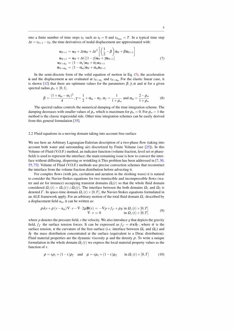
into a finite number of time steps tN such as t0 = 0 and tNmax = T . In a typical time step
∆ t = tN+1 − tN , the time derivatives of nodal displacement are approximated with:
uN+1 = uN +∆ tuN +∆ t2
[(1
2−β
)
uN +β uN+1
]
uN+1 = uN +∆ t [(1− γ)uN + γ uN+1]uN+α f
= (1−α f )uN +α f uN+1
uN+αm = (1−αm)uN +αmuN+1
(7)
In the semi-discrete form of the solid equation of motion in Eq. (5), the acceleration
u and the displacement u are evaluated at tN+α fand tN+αm For the elastic linear case, it
is shown [12] that there are optimum values for the parameters β ,γ,α and α for a given
spectral radius ρ∞ ∈ [0,1].
β =(1+αm −α f )
2
4,γ =
1
2+αm −α f ,α f =
1
1+ρ∞
and αm =2−ρ∞
1+ρ∞
(8)
The spectral radius controls the numerical damping of the time integration scheme. The
damping decreases with smaller values of ρ∞ which is maximum for ρ∞ = 0. For ρ∞ = 1 the
method is the classic trapezoidal rule. Other time integration schemes can be easily derived
from this general formulation [35].
2.2 Fluid equations in a moving domain taking into account free-surface
We use here an Arbitrary Lagrangian-Eulerian description of a two-phase flow (taking into
account both water and surrounding air) discretized by Finite Volume (see [25]). In this
Volume-of-Fluid (V.O.F.) method, an indicator function (volume fraction, level set or phase-
field) is used to represent the interface; the main remaining issue is how to convect the inter-
face without diffusing, dispersing or wrinkling it.This problem has been addressed in [7,30,
55,75]: Volume of Fluid (V.O.F.) methods use precise convection schemes that reconstruct
the interface from the volume fraction distribution before advecting it.
For complex flows (with jets, cavitation and aeration in the sloshing wave) it is natural
to consider the Navier-Stokes equations for two immiscible and incompressible flows (wa-
ter and air for instance) occupying transient domains Ωi(t) so that the whole fluid domain
considered Ω f (t) = Ω1(t)∪Ω2(t). The interface between the both domains Ω1 and Ω2 is
denoted Γ . In space-time domain Ω f (t)× [0,T ], the Navier-Stokes equations formulated in
an ALE framework apply. For an arbitrary motion of the total fluid domain Ω f described by
a displacement field um, it can be written as:
ρ∂tv+ρ (v− um)∇ · v−∇ ·2µD(v) = −∇p+ f Γ +ρg in Ω f (t)× [0,T ]∇ · v = 0 in Ω f (t)× [0,T ]
(9)
where p denotes the pressure field, v the velocity. We also introduce g that depicts the gravity
field, f Γ the surface tension forces. It can be expressed as f Γ = σκδΓ , where σ is the
surface tension, κ the curvature of the free-surface (i.e. interface between Ω1 and Ω2) and
δΓ the mass distribution concentrated at the surface (equivalent to a Dirac distribution).
Fluid material properties are the dynamic viscosity µ and the density ρ . To write a unique
formulation in the whole domain Ω f (t) we express the local material property values as the
function of ι :
ρ = ιρ1 +(1− ι)ρ2 and µ = ιµ1 +(1− ι)µ2 in Ω f (t)× [0,T ] (10)
6
where the characteristic function or fluid volume fraction ι is defined as:
ι(x, t) =
1, for x ∈ Ω1(t)0, for x ∈ Ω2(t)
(11)
Let us note that when the whole domain is filled with one fluid (ι = 1 ∈ Ω f ), the classical
Navier-Stokes equations in ALE framework appear2. The fluid volume fraction ι and the
mass distribution δΓ are linked by the following relation:
∇ι = δΓ n (12)
To close the set of equations we have to write the conservation of ι . When no reaction
between phases occurs, the fluid volume fraction evolves only by advection:
∂t ι +(v− um) ·∇ι = 0 (13)
The conservation equation system on the whole domain Ω f in d dimensions can be
written as a function of the 2d+2 unknowns: um, v, p and ι are the solution of equations (9)
and (10) are verified. Traditional Computational Fluid Dynamic programs solve the fluid
equations on a fixed (Eulerian) grid. This present a difficulty in fluid-structure interaction
problems because of moving domains at the fluid interface which follows the deformations
of the structure. The classical approach to overcome this difficulty is to consider the so-
called Arbitrary Lagrangian Eulerian (ALE) method where the whole grid is moved inside
the fluid domain, in trying to follow the movement of the boundary. However, this leads to
the difficulty of pertaining the quality and the validity of the fluid inner mesh for different
new shapes of the boundary This is solved by building a suitable map for the domain motion
given its interface displacement. The fluid displacement um is arbitrary inside the domain
Ω f , but on the boundary it has to fulfill the condition:
um = um on ∂Ω f (t)× [0,T ] (14)
Inside the fluid domain Ω f the fluid displacement is an arbitrary extension of um|∂Ω f:
um = Ext
(
um
∣∣∣∂Ω f
)
(15)
The latter is possible to construct by solving the Laplace smoothing equation:
∇ · (γ∇um) = 0 in Ω f (16)
This kind of Laplace smoothing equation is known to have some limitation when the defor-
mation of the fluid domain is governed by large rotations (e.g. see []). In our case it shows
sufficient quality performance when the diffusion coefficient is made spatially dependent
upon the distance to the fluid-structure interface.
The second major difference from solids concerns the favorite discretization technique
for fluid in terms of the Finite Volume Method. The latter will transform the weak form
of the continuous equations in (9) to (16) into a set of algebraic equations that can be
solved numerically. One of the goal of this work is to couple different codes, with dif-
ferent dicretization methods (FEM for solids and FVM for fluids). this keeping the main
trends of computational scientific software. Namely, as FVM, contrary to FEM, leads to
2 Note that the stability proof for coupled fluid-structure interaction problem given in Part I is for this
classical case

7
intrinsically conservative methods at the local stage they are often preferred in commercial
and non-commercial softwares (Phoenics, FLuent, FLow3D, Star-CD, Code Saturne, Open-
FOAM [44] are all FVM based). Moreover, there is a great number of reference books on
the subject, among them [63,25]. We are however aware that work is made in order to solve
fluid with Finite Elements (see for instance [18,29,27,54,36,65,72,73,69,79]).
The FV formulation can be written directly using an integrated form of the conservation
equation written in (9). Another possibility is to consider the restriction of the solution space
of weak form problems. For consistency with the structure sub-problem formulation we
chose to describe the FV strategy in latter framework. The weak form of the Navier-Stokes
equation can be written as [32], find (um, ι ,v, p) ∈ U ×I × V ×P , such that, for all
(δum,δι ,δv,δ p) ∈ U0 ×I0 ×V0 ×P0:
G f :=∫
Ω f
∇ · (γ∇um)δum +∫
Ω f
(∂t ι +(v− um)∇ι)δι∫
Ω f
ρ∂tv ·δv+∫
Ω f
ρ∇(v− um)⊗ v ·δv−∫
Ω f
∇ ·µ f D(v) ·δv
+∫
Ω f
p∇ ·δv+∫
Ω f
∇ · vδ p+[B.C. in a weak form]
= 0
(17)
where U , I , V and P are suitable functional spaces for for the solution fields.
For this method, the whole volume Ω f is divided into a set of of discrete elements,
here called discrete volumes (κ f ,e)e=1,nelcovering the whole domain (Ω f = ∪
nele=1κ f ,e) with-
out overlapping (∩nele=1κ f ,e = /0). For a Finite Element discretization, the solution spaces are
restricted to suitable spaces of piecewise polynomial functions over the set of discrete ele-
ments. For a Finite Volume discretization used herein, the test functions are chosen in the
space of characteristic discrete volume functions. For instance, the velocity can be approxi-
mated as:
Vh = V ∩
v
∣∣∣v|κ ∈ span(ικ),∀κ ∈ T
h(Ω f )
(18)
where ικ is the characteristic function of the element defined as:
ικ : Ω f −→
x −→
1 if x ∈ κ0 if x ∈ Ω/κ
(19)
The same kind of restriction holds for the solution spaces of equation (17). Therefore, the
function are piecewise constant by elements, and with the restriction of the weak formulation
reduces to: find (uhm, ι
h,vh, ph)∈U h×I h×V h×V h, such that,for all (δuhm,διh,δvh,δ ph)∈
U h0 ×I h
0 ×V h0 ×V h
0 : G f ((uhm, ι
h,vh, ph);δuhm,διh,δvh,δ ph) = 0 . The divergence terms in
equation (17) can be written in terms of flux at the boundary of volume controls using the
Gauss theorem. Hence, the weak formulation can be written as:
0 = ∑κ
∮
∂κdΓ · (γ∇um)
− [B.C.]
0 = ∑κ
∫
κ∂t ι +
∮
∂κdΓ · (v− um) ι
− [B.C.]
0 = ∑κ
∫
κρ∂tv+
∮
∂κρ dΓ · (v− um)⊗ v−
∮
∂κdΓ ·µ f D(v)+
∮
∂κp dΓ
− [B.C.]
0 = ∑κ
∮
∂κdΓ · v
− [B.C.]

8
where dΓ is the elementary surface vector. Note that there is no continuity requirement
for the solution (contrary to classical FE), and therefore the approximate solutions need
not to be defined at the interface. Their flux can be computed without being imposed by
the restriction of the solution space to the FV space. The only difficulty is now to build
an accurate representation of the fluxes at the boundaries from a piecewise constant field.
On each control volume, three levels of numerical approximations are applied to build the
boundary fluxes: interpolation to express variable values at the control volume surface in
terms of nodal values (depending on where the variable is stored); differentiation to build
convective and diffusive fluxes the value of the gradient of the quantity of interest – or at
least its approximation – is required; integration to approximate surface and volume integral
using quadrature formulæ.
The semi-discrete form of the discretized fluid problem can be written in a matrix form
as follows. The fluid mesh motion considers that um is imposed by the motion of the interface
u:
Rm(um;u) := Kmum −Dmu= 0 (20)
where Dm is a projection/restriction operator and Km governs the extension of the boundary
displacement (see Eq. (16)). The volume fraction ι , the d components of velocity v and
pressure p are coupled through a set of non-linear equations. Written in a matrix forms, it
gives the following semi-discrete problem:
R f (ι ,v f ,p f ;um) :=
Mι ι +Nι(v f − um)ιM f (ι)v f +N f (ι ,v f − um)v+K f (ι)v f +B f p f − f f (ι)
BTf v f
= 0 (21)
where Mι and Nι are the matrices associated to the advection problem of the fluid volume
fraction, M f is a positive definite mass matrix, N f is an unsymmetric advection matrix,
K f is the conduction matrix describing the diffusion terms, and B f is for the gradient ma-
trix, whereas f f is the discretized nodal loads on the flow. This matrix form also takes into
account the boundary conditions; special care has to be taken concerning the discretiza-
tion of boundary conditions – and especially normal flux – when using the Finite Volume
Method [31].
One way to solve the flow problem is to consider a monolithic solver handling all equa-
tions simultaneously. Another way is to consider a split between the mesh motion, the vol-
ume fraction advection, the momentum and the continuity equations, and to use an operator
split-like procedure often referred to the segregated approach [63]. This approach is favored
for its computational efficiency compared to the monolithic scheme. Indeed, even with a
simple fixed point iteration strategy its cost is less important than that of the monolithic ap-
proach for large size problems [25]. In the work presented herein, the segregated approach
will be used because of its efficiency.
Let us note that for a given motion of the fluid domain, the coupling between the mesh
deformation and the Navier-Stokes equation is weak, in the sense that no variable like ve-
locity v or pressure p influences the fluid domain deformation under imposed boundary
displacements. The coupling between the mesh motion problem and the fluid momentum
equation can therefore be ensured explicitly.
The only remaining question is the choice of velocity variation in the time step ∆ t =tN+1− tN . As the mesh motion is arbitrary and does not rely on any physical phenomenon, it
is a priori possible to take any velocity evolution on the window [TN ,TN+1] so that the initial
mesh deformation is equal to um,N and the final mesh deformation is equal to um,N+1.

9
The Geometric Conservation Law demands a numerical scheme to reproduce exactly
and independently from the mesh motion a constant solution. This condition can be found
in the literature for ALE formulation discretized either by the Finite Volume [16] or the
Stabilized Finite Element methods [26]. It is proved [19] that the velocity of the dynamic
mesh needs to be computed for all first and second-order time integration schemes (like
implicit Euler or Crank-Nicholson):
um =um,N+1 −um,N
∆ t(22)
The volume fraction function is supposed to be sharp at the interface between water and
gazs, and therefore, standard FV discretization that can be strongly diffusive cannot be ap-
plied, as they would smear the interface. One way to guarantee a sharp and bounded solution
is by using a numerical scheme designed for the multi-dimensional advection equation [55].
We will not enter into the details of such a treatment, but let us note that, in our case, the
treatment of the volume fraction requires time sub-cycles, since an explicit treatment re-
ferred to as MULES (Multidimensional Universal Limiter with Explicit Solution) is used
(see [75,7]).
For the coupling between the pressure equation and the momentum equlibrium, strat-
egy based upon ACM (Artificial Compressibility Method) [11], or pressure correction tech-
niques such as SIMPLE (Semi-Implicit Method for Pressure Linked Equations) [64,76] or
PISO (Pressure Implicit with Splitting of Operators) [42,43] are traditionally used in CFD.
They often rely on the use of suitable relaxation parameters [25] in order to reach conver-
gence for the stiff coupled problem. In [67], a comparison between ACM and pressure-
correction techniques is given and in [4], a comparison of two pressure-correction algo-
rithms showed the overall better performances of PISO algorithms over SIMPLE ones.
In this work, PISO algorithms are used to solve our CFD problem. The semi-discrete
form of the Navier-Stokes equation is discretized in time using implicit integration schemes
(the Euler implicit, or the second order Crank-Nicholson scheme). The discretized momen-
tum Eq. (21) is split into the following way when an implicit integration scheme is used:
A f (vN+1)vN+1 −H f (vN ,vN+1) =−B f pN+1 (23)
where A f stands for time derivative terms in a cell (and is therefore diagonal) and H f takes
into account all neighboring velocity and source terms in elements. The incompressibility
condition can be re-written in a discrete form using the previous split as:
BTf
1
A f (vN+1)B f pN+1 −BT
f
1
A f (vN+1)H f (vN ,vN+1) = 0 (24)
For the PISO algorithm, the coupling between the incompressibility condition and the
momentum equilibrium parts of the Navier-Stokes equation is assured in an iterative way.
It is not fully implicit, as corrective term of the velocity is introduced explicitly. Hence, in
the correction step, it is supposed that the influence of the transported term is negligible
compared to the pressure gradient correction terms. Therefore, even with an implicit time
integration scheme, the stability of the PISO algorithm remains conditional, and when the
Courant Number becomes too large (meaning that the transport due to the flow over a cell
is not well captured) the PISO algorithm fails to converge.

10
3 Space interpolation between solvers
The use of different discretization and time-integration schemes, for the fluid and the struc-
ture part, do not provide in general a matching mesh at the interface. This feature is taken
into account in the nonlinear stability analysis performed in the Part I of this paper by in-
terpolation matrix in the contraction parameter α . Furthermore, even for matching meshes,
as the geometries of the domains are not the same on both sides of the interface, an op-
timal numbering of the nodes can lead to different orders for the interface nodes. In the
example proposed herein, only this latter point is of interest. Last but not least, different
discretization techniques (Finite Element versus Finite Volume) or different order p of the
polynomials can be used for constructing solution to fluid-structure interaction problem. In
the domain of FE applied to mechanical engineering, extensive literature can be found on
how to build a consistent interpolation for both sub-problems at the interface [22]. For the
fluid-structure interaction problems, an interesting review can be found in [14]. For the sake
of simplicity, the use of Dirac functions has often been proposed [41,33].
In our approach, it was decided not to favor any particular mesh-based representation
at the interface, and even allow that the fluid problem can also be solved by a meshfree-
based method [61,13]. Namely, an interpolation strategy relying on radial basis function
is chosen herein. As suggested in [6], this method fits well with the current work where,
both sides of the problem are based on different approximation techniques. First, for the
structure we employ the FE approximation that requires values imposed at the nodes and
gives in return nodal values as answers. Second, in the FV discretization for the fluid part,
the fields at the interface are defined at the center of the cells, and not at the nodes as it
is done for FE. However, as the client has no reason to know the connectivity table of the
coupled component nor the faces centers coordinates, it was decided to interpolate the fields
internally in ofoam-2 and to set or get them at the points of the interface.
The Steklov-Poincare operators for the fluid and the structure (described in Part I of this
paper and based on the FE and FV solvers) request imposed boundary values at the nodes
placed interface, and provide the values, for potentially different nodal points x f and xs.
The interpolation step from fluid to structure consist in solving a linear system as explained
subsequently.
Let us consider that the displacement vector at the Ns solid nodes (xs,i)i=1...Ns is given
as (us,i)i=1...Ns . We want to build the interpolation of this displacement field at the N f fluid
nodes in order to impose the fluid mesh motion as needed in ALE fluid computations. An
interpolation for each scalar field of the projected displacements in one of the Cartesian
directions has then to be built. This scalar field is denoted as ui = u(xs,i) at each points, and
the interpolation has to be performed d times for each vector field of dimension d.
Then the interpolation at a point x takes the form:
u(x) =Ns
∑i=1
ciΦ(x− xs,i) (25)
where Φ is a fixed basis function which is radial with respect to the Euclidian distance, i.e.:
Φ(x) = Φ(‖x‖2) = Φ(
√√√√
d
∑i=1
x2i ) (26)
11
The coefficients ci are determined by the interpolation condition:
u j =Ns
∑i=1
ciΦ(xs, j − xs,i) (27)
Thus, for interpolation of any field to interpolate, the coefficients ci have first to be
computed as the inverse of the following relation:
Mi jc j = u j (28)
where the interpolation matrix entries are computed as:
Mi j = Φ(xs, j − xs,i)
The last step is to compute the interpolated field by using the expression given in Eq. (25).
The choice of the radial basis function is governed by the requirement that the influence
of a center has to be smaller when the distance to an evaluation node increases. Elsewhere,
the global character of the radial basis function tends to smooth out all local effects. Another
desirable property is to use the functions with compact support which results with a sparse
interpolation matrix. In [6], a comparison between different smooth compact radial basis
functions for field transfer at the interface is given. In this work, global radial basis function
are used in the exponential form:
Φ(x) = exp−‖x‖
h(29)
where h is a characteristic distance between points.
The Interpolator implementation is described in [46]. The advantage of the compo-
nent use is the possibility to plug-in any interpolation software to the fluid-structure inter-
action framework that matches the Component Interface. The inverse problem of the full
matrix Mi j is here relying on the lapack or the Intel Math Kernel Library; the cost of such
an operation is around N3, but as the interface d-o-f are by far less than number of d-o-f
for each subproblem, in general this cost cannot be the bottleneck of the computations. One
of the advantages of the proposed approach is that the interpolation is exact for matching
nodes. It can be used without any lack of precision in a generic way for matching meshes
where the ordering is not the same for both subproblems.
4 COupling the software COmponents by a Partitioned strategy (cops) and parallel
computations
4.1 Software coupling applied to fluid-structure interaction
Coupling a fluid code and a structure code in order to produce the code for solving the
fluid-structure interaction problem is carried by master coupling approach, where a master
code sends request and receive data from the coupled software. Traditionally this approach
is quite intrusive, and imposes new developments inside the software. However, the use of
component technology with the middleware CTL (see [62]) eliminates the difficulties in the
master coupling approach. We will here insist on two points: the development of a compo-
nent based upon an existing code requires a very good understanding of its architecture, and
a deep knowledge of the physics behind. However, once the component is developed, it can
actually be used as a black box.
12
The COupling COmponents by a Partitioned Strategy (cops) provides a generic imple-
mentation of the explicit and implicit DFMT-BGS algorithms for fluid-structure interaction.
The key idea is to re-use existing codes, here FEAP for structures and OpenFOAMfor fluids, as
elementary bricks to build upon the CTL components.
We note that cops itself is a component and has been successfully re-use in [2] for
sequential multi-scale approach to solving fluid-structure interaction problem. Dependency
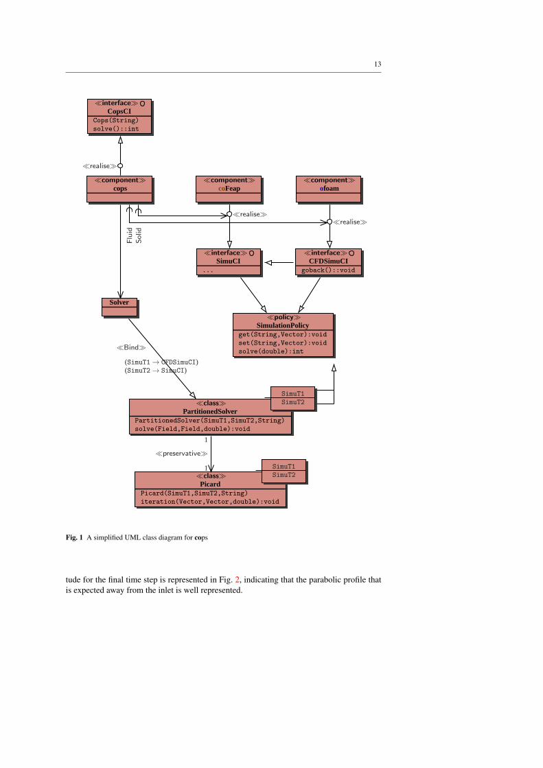
graph of cops component is presented by a general overview of its architecture given in
UML syntax in Fig. 1.
The interface, defined in a .ci file, is realized by a C++ class named cops. The main
routine calls the coupling component, providing the path where the control file associated to
cops lies. The coupling component cops instantiates two sub-solvers, the one of coFeap for
the structure and another of ofoam-2 for the fluid problem and with a partitionedSolver
binding the two subproblems. PartitionedSolver is a template class that couples any com-
ponent matching a SimuCI or a CFDSimuCI where method is necessary to build the Steklov-
Poincare operators, and optionally goback in time if sub-iterations of one subproblem in
implicit computations is asked for.
The PartitionedSolver instantiates a Picard method that is in charge of one Picard
iteration upon the coupled subproblem. One Picard iteration allows to determine the new
residual needed to check the convergence of the DFMT-BGS solver. The Picard class itself
relies on a template SteklovPoincare class.
4.2 Performance Comparison between system calls and file reading/writing for the fluid
component
In its first implementation (see [50]), the ofoam component architecture was based on file
reading and system calls. Behind the CFDSimu.ci interface is implemented a class that reads
output files from OpenFOAM and uses system calls in order to perform computation. This
implementation has the advantage of being not intrusive at all, since the component depends
neither on header files nor on OpenFOAM libraries. However, the slow execution speed for this
kind of implementation makes it prohibitively expensive for any large scale computations.
The second implementation described herein above concerns a component directly linked
to OpenFOAM, and it has the major advantage of working than the first. In order to evaluate
the performance gain obtained with the new implementation, we compare the CPU time
required by the call of methods of each component (ofoam-1 – based on file reading – and
ofoam-2 – the wrapper class and component build around OpenFOAM) on the same test case.
The latter concerns a Newtonian flow in a cylinder for fully 3D case. The chosen di-
mensions of the cylinder: diameter 1m and length 10m. The velocity on the inlet is imposed
as being uniform (10m.s−1), whereas at the outlet, the pressure gradient is set to 0. Perfect
wall conditions (zero velocity) are applied to tube walls. We consider following values for
material properties: density ρ = 1.0kg.m−3 and dynamic viscosity µ = 0.01m2.s−1. The
numerical simulations spans time interval from t = 0s to t = 0.01s. The discretization in
space is carried out by second order Finite Volume approximation. For time discretization,
the implicit Euler scheme with dt = 0.001s is applied. The algorithm chosen to handle the
computations with incompressibility constraint is based on PISO [25]. At each time step,
two outer corrections are performed to ensure the pressure velocity coupling. The solvers
for the fluid velocity and pressure fields are based on PBiCG and PCG respectively.
The computations are performed for meshes with 9×10³, 72×103 and 576×103 cells
(the number of d-o-f equals roughly 4 times the number of cells). The velocity field magni-
13
≪interface≫CopsCI
Cops(String)
solve()::int
≪component≫cops
≪component≫coFeap
≪component≫ofoam
≪interface≫SimuCI
...
≪interface≫CFDSimuCI
goback()::void
Solver
≪policy≫SimulationPolicy
get(String,Vector):void
set(String,Vector):void
solve(double):int
≪class≫PartitionedSolver
PartitionedSolver(SimuT1,SimuT2,String)
solve(Field,Field,double):void
≪class≫Picard
Picard(SimuT1,SimuT2,String)
iteration(Vector,Vector,double):void
SimuT1
SimuT2
SimuT1
SimuT2
Solid
Fluid
≪realise≫
≪realise≫≪realise≫
≪preservative≫
1
1
≪Bind≫
(SimuT1 → CFDSimuCI)(SimuT2 → SimuCI)
Fig. 1 A simplified UML class diagram for cops
tude for the final time step is represented in Fig. 2, indicating that the parabolic profile that
is expected away from the inlet is well represented.

14
Fig. 2 Velocity field magnitude in the cylinder in m.s−1
cells 9×10³ 72×103
version ofoam-2 ofoam-1 ofoam-2 ofoam-1
met
ho
ds
init 5.03×10−01 5.50×10−01 3.96×10+00 3.79×10+00
getnodes 1.44×10−04 1.75×10−02 3.10×10−04 1.34×10−01
set 5.07×10−05 5.27×10−04 8.92×10−05 1.46×10−03
solve 6.10×10−01 9.66×10−01 1.60×10+01 1.73×10+01
get 2.00×10−04 3.48×10−02 6.29×10−04 2.68×10−01
total 1.17×10+00 1.89×10+00 2.00×10+01 2.19×10+01
cells 576×103 4608×103
version ofoam-2 ofoam-1 ofoam-2 ofoam-1
met
ho
ds
init 4.52×10+01 4.13×10+01 5.79×10+02 5.50×10+02
getnodes 8.81×10−04 1.10×10+00 3.18×10−03 8.41×10+00
set 2.06×10−04 4.74×10−03 6.33×10−04 1.78×10−02
solve 1.89×10+02 1.98×10+02 1.87×10+03 1.94×10+03
get 2.22×10−03 2.09×10+00 8.64×10−03 1.77×10+01
total 2.35×10+02 2.44×10+02 2.45×10+03 2.53×10+03
Table 1 Performance comparison between ofoam and ofoam-2 in terms of CPU time for each method given
in seconds; the latter has been measured using the CTL profiler (CTL Profile).
The overall performance of ofoam-1 and ofoam-2 components as expected (see Table 1).
The ofoam-1 component based on file reading will be intrinsically less efficient for methods
that require intrinsically a lot of data exchange compared to the computation cost (meth-
ods get nodes, pressure and velocity and set velocity and mesh displacements), since the
speed of access to data by opening and reading files written on the hard drive cannot com-
pete with a direct access to the memory. However, for all the methods that require a lot of
computations, the performances of ofoam-1 and ofoam-2 implementations are comparable
and mainly depends on the implementation of OpenFOAM itself, as the time spent in data
exchange is very small compared to the one spent in the computation, especially for a huge
number of d-o-f.

15
In Fig. 3, the bottleneck of a fluid computation pertains, as expected, to the problem
solving (matrix inversion for any method used). Note that the solve method is a bit faster
for ofoam-2 implementation since there is no need for the software to reload data before
performing computation. Thus, the slight advantages offered in terms of CPU time does not
alone justify the choice of building a new component ofoam-2. Rather the possibility of
reusing any class developed in the OpenFOAM project provides a better argument in favor of
the new implementation
4.3 Parallel CFD Component Performance and nested parallelization
For most fluid-structure interaction problems, the bottleneck of performances are flow com-
putations. For instance, in the problem presented in this article, where the fluid domain
surrounds the structure, more than 95% of the computational time is spend in the fluid com-
putation. Therefore, even if the parallelization of the coupling algorithm is of interest, this
can result in sufficient increase of efficiency only in the case if the fluid and the structure
computations require the same CPU time. For all other cases we will used the nested paral-
lelization, where the parallel coupling algorithm can accommodate parallel fluid computa-
tion. The implementation of nested parallel coupling algorithms can then be accomplished
with CTL in a quite straightforward manner by using a certain number of instance of the
ofoam-2 component controlled by the CTL.
The performance of the parallel version of the ofoam-2 component is tested on the same
problem of flow in a cylinder. For space discretization and the chosen mesh is handled by
METIS [47] in each sub-domain with the same weight (Fig. 4). In each computation, the
bottleneck is computation of the flow evolution between two time steps. The computational
time reported in this section is the average time T CPU required to solve one time step of
the given problem and to write the associated results. The initialization time is therefore not
taken into account.
We consider the main indicator to measure the performance of the nested parallelization
to be the speed-up χ defined as:
χ =T CPU
1
T CPUN
(30)
where T CPU1 is the computational time for the problem solved on one processor and T CPU
N
for N processors. A linear speed-up: it means that taking N processors, one expects to divide
the computational time by N, cannot be obtained with ofoam-2. Namely, the communication
between processes, that is highly linked to size of interfaces, has to be taken into account.
For this reason, the notion of efficiency can be introduced in hoping to have it close to 1:
ξ =T CPU
1
N ×T CPUN
(31)
We tested the nested parallel computations on the same multi-processor machine or on
a cluster architecture where computers communicate throughout a network, and we report
both set of results. We underline that the given results are empha priori different from the one
obtained comparing the parallelization of OpenFOAM, as the communication is made between
CTL components.

16
Tim
e(s
)
10−1
101
103
105
7·103 7·104 7·105 7·106
ofoam 1
rs
rs
rs
rs
rs
ofoam 2
bc
bc
bc
bc
bc
init
Tim
e(s
)
10−4
10−2
100
102
7·103 7·104 7·105 7·106
ofoam 1
rs
rs
rs
rs
rs
ofoam 2
bcbc
bc
bc
bc
get
(no
des
)
Tim
e(s
)
10−4
10−2
100
102
7·103 7·104 7·105 7·106
ofoam 1
rs
rs
rs
rsrs
ofoam 2
bc
bc
bc
bc
bc
get
(pre
ssu
re)
Tim
e(s
)
10−5
10−3
10−1
101
7·103 7·104 7·105 7·106
ofoam 1
rsrs
rs
rs
rs
ofoam 2
bcbc
bc
bc
bcset
(vel
oci
ty)
Tim
e(s
)
10−1
101
103
105
7·103 7·104 7·105 7·106
ofoam 1
rs
rs
rs
rs
rs
ofoam 2
bc
bc
bc
bc
bc
difference
b
b
b
b
b
solve
Number of cells
Fig. 3 Performance comparison between some ofoam and ofoam-2 methods for different mesh refinements.
17
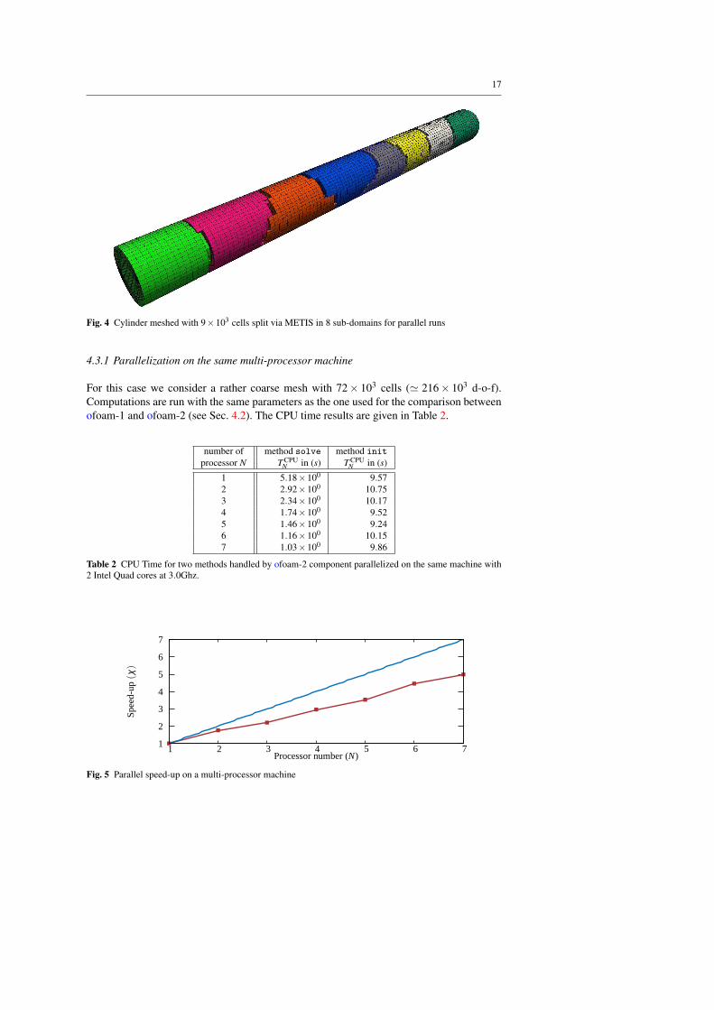
Fig. 4 Cylinder meshed with 9×10³ cells split via METIS in 8 sub-domains for parallel runs
4.3.1 Parallelization on the same multi-processor machine
For this case we consider a rather coarse mesh with 72× 103 cells (≃ 216× 103 d-o-f).
Computations are run with the same parameters as the one used for the comparison between
ofoam-1 and ofoam-2 (see Sec. 4.2). The CPU time results are given in Table 2.
number of method solve method init
processor N T CPUN in (s) T CPU
N in (s)
1 5.18×100 9.57
2 2.92×100 10.75
3 2.34×100 10.17
4 1.74×100 9.52
5 1.46×100 9.24
6 1.16×100 10.15
7 1.03×100 9.86
Table 2 CPU Time for two methods handled by ofoam-2 component parallelized on the same machine with
2 Intel Quad cores at 3.0Ghz.
1
2
3
4
5
6
7
1 2 3 4 5 6 7
Spe
ed-u
p(χ)
Processor number (N)
rs
rsrs
rs
rs
rs
rs
Fig. 5 Parallel speed-up on a multi-processor machine

18
The graphic illustration of the results is given in Fig. 6, showing that efficiency of nested
parallel computing is maintained around 0.7, even with 7 processors. Similarly, in parallel
computation we 7 processors one can observe a Speed-up (Fig. 5) of around 5 times.
0.2
0.4
0.6
0.8
1
1 2 3 4 5 6 7
Effi
cien
cy(ξ
)
Processor number (N)
rs
rs
rs rsrs
rsrs
Fig. 6 Parallel efficiency on a multi-processor machine
However, the question of the representative value of this computation can be raised, as
the mesh size is maybe not big enough and compared to the time spend in the solving, the
communication cost between processes may not be negligible.
number of reference compact transfer standard transfer
cells T CPU1 in (s) T CPU
6 in (s) T CPU6 in (s)
9×10³ 3.91×10⁻¹ 1.38×10⁻¹ 4.52×10⁻¹
30375 1.54×100 5.27×10⁻¹ 7.39×10⁻¹
72×103 5.18×100 1.16×100 1.27×100
243×103 2.84×101 8.14×100 6.97×100
576×103 1.07×10² 4.13×101 3.17×101
4608×103 1.66×10³ 8.42×10² 7.13×10²
Table 3 CPU Time for the solve for different meshes 3.0Ghz with standard and compact transfer
For that reason, we compute the flow in a cylinder problem for different mesh refine-
ments – from 27×103 to roughly 18×106 d-o-f – on one processor, and then repeat parallel
computations on 6 processors. Here is represented the computational time spent for the solve
method with direct and compressed transfers between the processes. In compressed transfer,
each double is converted into a float, leading to a small loss of accuracy.
These results are illustrated in Fig. 7 in terms of efficiency of the parallel computation on
6 processors as a function of number of cells for different mesh refinement. One observes a
decrease in the performance for coarser grids, as for these cases the communication between
processes is not negligible. This is even more noticed for standard transfer when one chooses
not to compress the double into float.
Moreover, we also observe a decrease in the performance for finer meshes. This is the
consequence of imposing the incompressibility conditions, which requires more iterations
in a parallel than in a serial run. Namely, it is known that state solver convergence is affected
by running in parallel as the preconditioning and smoothing operations in the cells adjacent
to the boundaries are less effective, and lead to a small increase in the number of iterations.
Moreover, in any such case, decreasing the accuracy when the values between processes are
transmitted with compact transfer is not a good choice, since the gain obtained on the com-
19
0.2
0.4
0.6
0.8
1
7·103 7·104 7·105 7·106
Effi
cien
cy(ξ
)
Number of cells
compact transfer
rs rs
rs
rs
rs
rs
rs
standard transfer
bc
bc
bcbc
bc
bc
bc
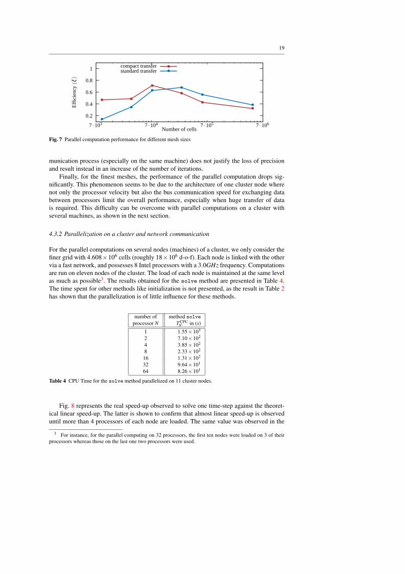
Fig. 7 Parallel computation performance for different mesh sizes
munication process (especially on the same machine) does not justify the loss of precision
and result instead in an increase of the number of iterations.
Finally, for the finest meshes, the performance of the parallel computation drops sig-
nificantly. This phenomenon seems to be due to the architecture of one cluster node where
not only the processor velocity but also the bus communication speed for exchanging data
between processors limit the overall performance, especially when huge transfer of data
is required. This difficulty can be overcome with parallel computations on a cluster with
several machines, as shown in the next section.
4.3.2 Parallelization on a cluster and network communication
For the parallel computations on several nodes (machines) of a cluster, we only consider the
finer grid with 4.608×10⁶ cells (roughly 18×106 d-o-f). Each node is linked with the other
via a fast network, and possesses 8 Intel processors with a 3.0GHz frequency. Computations
are run on eleven nodes of the cluster. The load of each node is maintained at the same level
as much as possible3. The results obtained for the solve method are presented in Table 4.
The time spent for other methods like initialization is not presented, as the result in Table 2
has shown that the parallelization is of little influence for these methods.
number of method solve
processor N T CPUN in (s)
1 1.55×10³
2 7.10×10²
4 3.85×10²
8 2.33×10²
16 1.31×10²
32 9.64×101
64 8.26×101
Table 4 CPU Time for the solve method parallelized on 11 cluster nodes.
Fig. 8 represents the real speed-up observed to solve one time-step against the theoret-
ical linear speed-up. The latter is shown to confirm that almost linear speed-up is observed
until more than 4 processors of each node are loaded. The same value was observed in the
3 For instance, for the parallel computing on 32 processors, the first ten nodes were loaded on 3 of their
processors whereas those on the last one two processors were used.

20
previous section, when the parallelization was done on the processors of the same machine,
thus indicating some limitation of the architecture of the cluster nodes.
1
2
4
8
16
32
1 2 4 8 16 32 64
Spe
ed-u
p(χ)
Processor Number (N)
rs
rs
rs
rs
rs
rsrs
Fig. 8 Parallel computation speed-up for runs on different cluster nodes
The efficiency of the parallel computing, as shown in Fig. 9 remains around optimum
value of 1 before it starts decreasing. Note that the efficiency for parallel computation in a
small number of cluster nodes is above the theoretical optimum. This is due to the fact that
less data need to be handled by the memory on each nodes. It is also of interest to compute
the CPU time for the same range of mesh size as the one given in Table 5.
0.2
0.4
0.6
0.8
1
1 2 4 8 16 32 64
Effi
cien
cy(ξ
)
Processor Number (N)
rs
rs
rs
rs
rs
rs
rs
Fig. 9 Parallel computation efficiency for runs on different cluster nodes
We also computed the efficiency obtained for different mesh sizes and present the results
in Fig. 10. For this computation, each grid is split into 6 sub-domains, then solved on 6
different machines. Contrary to the phenomenon observed for parallel runs on the same
machine (Fig. 7), the expected gain in efficiency is observed with increasing number of d-o-
f and parallel computation on different machines. In other words, the bigger is the mesh, the
more efficient is the parallel computation, since the communication between components
then remains small compared to the time spent for solving the problem.
Handling data transfer with compacting the exchanged values from double to float for
is not advantageous for all computations of the studied flow case. Namely, the speed-up in
communication for compact transfer is diminished by the loss in accuracy that leads to more
iterations to smooth the values and precondition the solvers, especially near the sub-domain
boundaries.

21
number of reference standard transfer compact transfer
cells T CPU1 in (s) T CPU
6 in (s) T CPU6 in (s)
9×10³ 3.83×10⁻¹ 2.74×10⁻¹ 3.33×10⁻¹
30×103 1.55×100 5.44×10⁻¹ 6.38×10⁻¹
72×103 4.38×100 1.16×100 1.29×100
243×103 2.45×101 4.02×100 4.58×100
576×103 8.11×101 1.28×101 1.57×101
4608×103 1.55×10³ 2.59×10² 2.90×10²
Table 5 CPU Time for the solve for different meshes with standard and compact transfer
0.2
0.4
0.6
0.8
1
7·103 7·104 7·105 7·106
Effi
cien
cy(ξ
)
Number of cells
compact transfer
rs
rs
rs
rs rs rs
rs
standard transfer
bc
bc
bc
bcbc
bcbc
Fig. 10 Parallel computation performance on six different cluster nodes for increasing mesh sizes from 216×103 to 18×106 d-o-f
5 Application examples
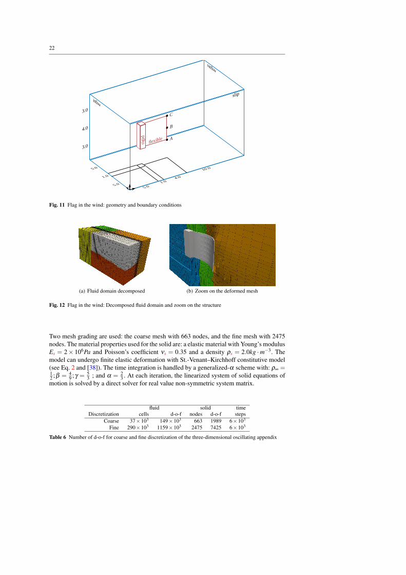
5.1 Three-dimensional flag in the wind
This problem was recently introduced in [77], as a 3D generalization of the oscillating ap-
pendix problem discussed in Part I of this work. It can be thought of as a simplified three-
dimensional model for the interaction of a flag with an incompressible viscous flow. All di-
mensions and the geometry of the problem, defined in Fig. 11, are given in cm. The material
properties for the fluid are: the mass density ρ f = 1.18×10⁻³kg.cm−3 and fluid kinematic
viscosity ν f = 0.1542cm.s−2.
The fluid problem is discretized with FV method, and then split in 6 sub-domains by
METIS software tool in order to performs parallel computations (see Fig. 12). The chosen
boundary conditions, specified in Fig. 11. are as follows: for lateral walls of the fluid domain,
the velocity boundary condition allows for slipping; at the inflow, a constant velocity is
imposed with v = (100cm.s−1,0,0); Zero gradient pressure is specified at the outflow.
In order to smooth the first steps of the fluid-structure interaction computations, we
do not start from the rest, but rather perform the fluid only computation from t = −2s
to t = 0s, with the inflow velocity increasing in a smooth way the velocity according to:12
(sin
(π(
t+12
))+1
)The fluid-structure interaction will start at t = 0s. All the points of the
fluid mesh will move in the ALE strategy, with their motion governed by a smoothing pro-
cess based on the Laplacian operator and a diffusivity coefficient whose value depends on
the distance to the appendix. The fluid discretization techniques and solvers are equivalent
to the one used in the two-dimensional example.
In the previous computation of this problem achieved in [77], the discretization of the
structure problem is performed by shell finite elements. Three-dimensional elements with
quadratic shape functions are used herein, with each elements therefore containing 27 nodes.
22
5.01.0
4.0
10.0
5.0
1.0
5.0
3.0
4.0
3.0
b
b
b
inflow
outflow
slip
flexible A
B
C
rigid
Fig. 11 Flag in the wind: geometry and boundary conditions
(a) Fluid domain decomposed (b) Zoom on the deformed mesh
Fig. 12 Flag in the wind: Decomposed fluid domain and zoom on the structure
Two mesh grading are used: the coarse mesh with 663 nodes, and the fine mesh with 2475
nodes. The material properties used for the solid are: a elastic material with Young’s modulus
Es = 2× 10⁶Pa and Poisson’s coefficient νs = 0.35 and a density ρs = 2.0kg ·m−3. The
model can undergo finite elastic deformation with St.-Venant–Kirchhoff constitutive model
(see Eq. 2 and [38]). The time integration is handled by a generalized-α scheme with: ρ∞ =12;β = 4
9;γ = 5
3; and α = 2
3. At each iteration, the linearized system of solid equations of
motion is solved by a direct solver for real value non-symmetric system matrix.
fluid solid time
Discretization cells d-o-f nodes d-o-f steps
Coarse 37×103 149×103 663 1989 6×10³
Fine 290×103 1159×103 2475 7425 6×10³
Table 6 Number of d-o-f for coarse and fine discretization of the three-dimensional oscillating appendix
23
The total number of d-o-f for the coupled problem is given in Table 6 for both coarse
and fine mesh. The computation is carried out with a coupling time step of 1× 10⁻³s for
each mesh. The coupling scheme used is DFMT-BGS with Aitken’s relaxation. The initial
relaxation parameter is ω = 1.0. The chosen value of the residual tolerance for coupled sim-
ulation is: ‖r(k)N ‖2 ≤ 1×10⁻⁷. In this work, only fluid-structure computations with implicit
DFMT-BGS coupling algorithm are performed. However, it should have been possible to
consider explicit coupling, as for the two-dimensional version of this problem as presented
in Part I, since the convergence of implicit scheme with the predictor of second order is fast
and requiring no more than 4 to 5 iterations per time step.
Tim
et=
4.3
5s
Tim
et=
5.1
0s
Tim
et=
5.9
5s
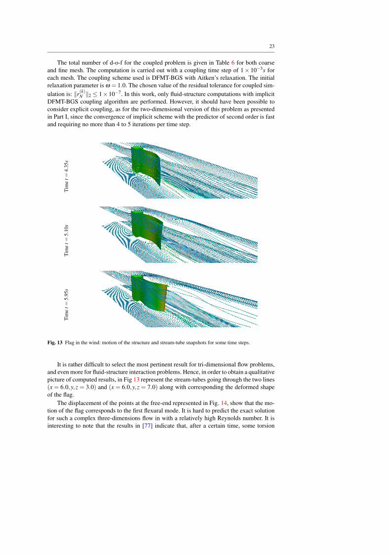
Fig. 13 Flag in the wind: motion of the structure and stream-tube snapshots for some time steps.
It is rather difficult to select the most pertinent result for tri-dimensional flow problems,
and even more for fluid-structure interaction problems. Hence, in order to obtain a qualitative
picture of computed results, in Fig 13 represent the stream-tubes going through the two lines
(x = 6.0,y,z = 3.0) and (x = 6.0,y,z = 7.0) along with corresponding the deformed shape
of the flag.
The displacement of the points at the free-end represented in Fig. 14, show that the mo-
tion of the flag corresponds to the first flexural mode. It is hard to predict the exact solution
for such a complex three-dimensions flow in with a relatively high Reynolds number. It is
interesting to note that the results in [77] indicate that, after a certain time, some torsion

24
-1
-0.5
0
0.5
1
0 1 2 3 4 5 6
Dis
plac
emen
t(d y
inm
)
Time (s)
ABC
(a) Oscillating 3D Appendix: extremity displacements for points A = (10.0,5.5,3.0), B =(10.0,5.5,5.0) and C = (10.0,5.5,7.0).
-0.6
-0.4
-0.2
0
0.2
0.4
0.6
0 1 2 3 4 5 6
Dis
plac
emen
t(d y
incm
)
Time (s)
C
FEMs+SFEMf DFMT-BGS
(b) Oscillating 3D Appendix: extremity displacements for points C comparison with [77] (DFMT-BGS
coupling FEM for structure and stabilized FEM for fluid).
Fig. 14 Displacement of structure extremity
modes occur in the flag, that could not be confirmed here at the same Reynolds number.
Consequently, the motion amplitude presented herein is around 4 times bigger than the one
obtained in [77]. Our results are more in agreement with the ones provided for 2D version
of the same problem (see [18,58,78]) with a flexible appendix.
5.2 Three-dimensional sloshing wave impacting a flexible structure
In [49], we have studied and validated our coupling framework in application free-surface
flow in interaction with non-linear structures. The problem presented herein emphasize the
3D capacities of our approach as well as the possibility to deal with complex flow. This
example is a simplified representation of a dam-breaking event that brings about the sloshing
wave impact on a flexible structure standing in its way, as presented in Fig. 15. At initial
time t = 0s, a three-dimensional water column starts falling down under the gravity loading.
Spreading further at a later time, it hits the obstacle which is a slender plate-like solid body
made of elastic material that can undergo large deformations. The dimension of the problem
and the imposed boundary conditions are given in Fig. 15.
In order to prevent that the water will bounce-back and again hit the structure after
breaking on the walls, only the left and bottom planes of the fluid domain are defined as
non-slipping walls, while the others are defined with atmospheric boundary condition for
the pressure.
The material properties are chosen as follows: for the high density fluid (the water)
the density and the kinematic viscosity are ρ f ,1 = 1×10³kg.m−3 and ν f ,1 = 1×10⁵m.s−1,

25
g
Ωf,1
Ωf,2
Ωs
146
14012
286
146
292
146
80
80
292
292
Fig. 15 Three-dimensional wave impacting an obstacle: geometry and boundary conditions
whereas for the low density fluid (the air in the remaining part of the domain) ρ f ,2 = 1kg.m−3
and ν f ,2 = 1×10⁶m.s−1 . The mesh motion problem is solved using a Laplacian smoothing
material where the diffusion coefficient is a quadratic inverse function of the distance to the
interface between structure and fluid.
The fluid domain is discretized with Finite Volume cells covering always the complete
domain either by one phase or by the other. The computations are performed for two dif-
ferent meshes with the chosen discretization and the number of cells given in Table 7. An
explicit-implicit algorithm is used to compute the two phase flow evolution from the corre-
sponding the Navier-Stokes equations. In the Volume of Fluid (V.O.F.) method used herein
(see [30]), an indicator function (volume fraction, level set or phase-field) is used to repre-
sent the phases; leaving only the remaining issue on how to convect the interface without
diffusing, dispersing or wrinkling it. This is particularly troublesome when the volume frac-
tion is chosen as an indicator function because the convection scheme has to guarantee that
the volume fraction stays bounded, with the values that remain within its physical bounds
of 0 and 1. We here follow the idea proposed in [7]: Volume of Fluid (V.O.F.) method using
convection schemes that reconstructs the interface from the volume fraction distribution be-
fore advecting it. The equation associated with the characteristic function is solved with an
explicit time integration scheme whereas the remaining terms are solved with implicit time
integration schemes (see [75,7]). The fluid is handled by second order space discretization
with a Van Leer limiter used for the advection terms, and the implicit Euler time-integration
scheme. Note that small time steps are required for the explicit solution of the phase function

26
indicator equation, as well as the half-implicit nature of the coupling between the momen-
tum predictor and the pressure corrector. At this scale of modelling it is not required to
consider surface tension between the two fluids.
The structure model is constructed by using three-dimensional elements with quadratic
shape functions, where each element has 27 nodes. The material properties used herein cor-
respond to a neo-Hookean elastic material with Young’s modulus Es = 1×10⁶Pa, Poisson’s
ratio νs = 0, and a density ρs = 2500kg ·m−3, The chosen model an represent finite de-
formation. The time integration is carried out by a Generalized-α scheme with the chosen
parameters as ρ∞ = 12
β = 49, γ = 5
3and α = 2
3. The total number of d-o-f given in Table 7
for both the coarse and fine discretization.
fluid solid number of
Discretization cells d-o-f nodes d-o-f time steps
Coarse 13×103 63×103 363 1.1×10³ 1×10⁵
Fine 104×103 520×103 2205 6.6×10³ 1×10⁵
Table 7 Number of d-o-f for coarse and fine discretization of the three-dimensional dam-breaking problem
The computation of the coupled problem is carried out by an iterative scheme. The
results of fluid and structure computations are matched for a time step of 1× 10⁻⁴ for the
coarse and 2× 10⁻⁵ for the fine discretization. The coupling scheme is DFMT-BGS with
Aitken’s relaxation with the initial parameter ω = 0.25 and the predictor of order 1. The
absolute tolerance for coupled computation is equals to:
‖r(k)N ‖ ≤ 1×10⁻⁶ (32)
0
1
2
3
4
5
0 0.2 0.4 0.6 0.8 1
Itera
tion
num
ber
Time (s)
Fig. 16 Number of iterations in order to make the DFMT-BGS algorithm converge for the three-dimensional
dam-breaking problem
The number of iterations required to reach the convergence criteria is given in Fig. 16.
Note that there is no coupling iteration before the water hits the structure (the effect of
air flow can almost be deemed negligible with respect to the structure). During the water-
structure contact the number of iteration depends on chosen the discretization density. In
reaching the opposite wall, the water does not rebound on the wall but simply flows away,
which again does not require any iteration.
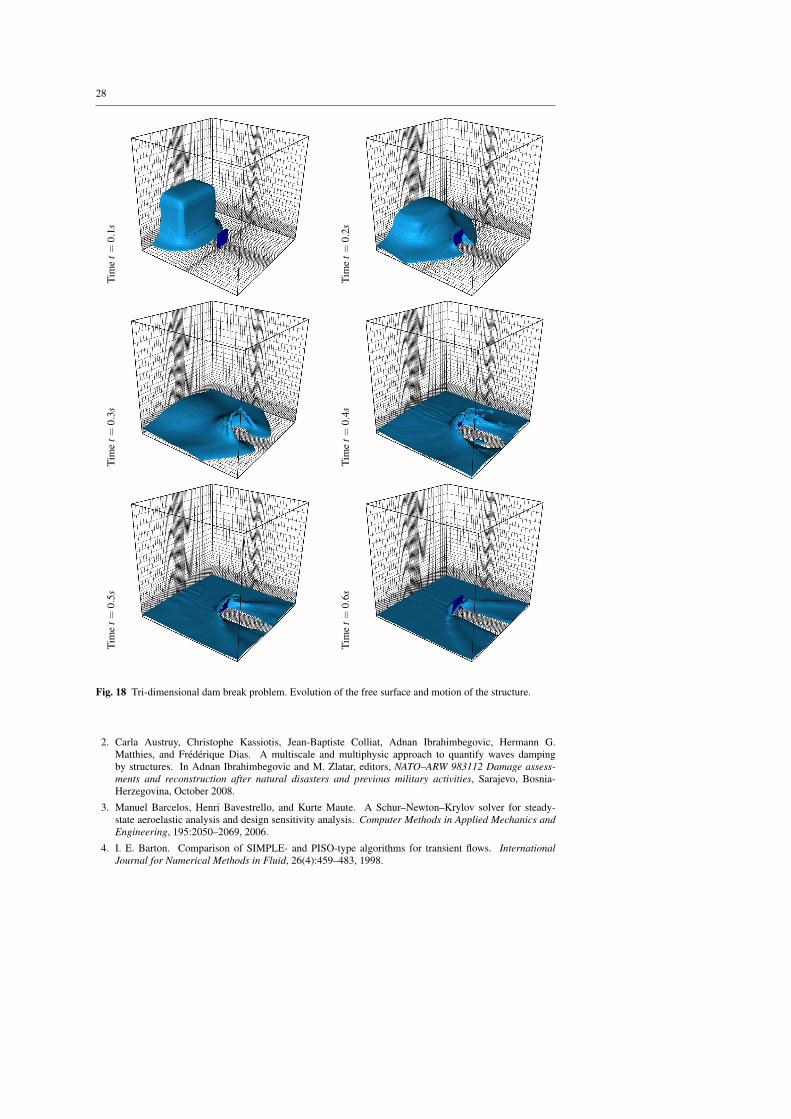
In Fig. 18, the water or high density fluid domain is represented, as well as some part
of the fluid mesh and the structure displacement. The first 0.1s of the simulations, the water

27
column falls under the gravity loading. There is no effect whatsoever on the structure until
the high density flow reaches its bottom. The maximum amplitude of the motion is obtain at
t = 0.25s, before the solid comes back to free-vibration phase.
-1
0
1
2
3
4
5
0 0.2 0.4 0.6 0.8 1
Dis
plac
emen
t(cm
)
Time (s)
coarse meshfine mesh
Fig. 17 Three-dimensional dam break example: obstacle displacement measured at the center of the top face
In Fig. 17 the motion of the free-end of the obstacle is plotted. Contrary to the two-
dimensional version of this example presented in [49], small drops of high density fluid are
not interacting with the obstacle after the main shock. Therefore, the motion of the solid part
remains rather well described even with the coarsest grid.
6 Conclusion
We propose in this work a solution approach to fluid-structure interactionproblems that al-
lows coupling different space discretization methods, such as FE for structures and FV for
fluids. As illustrated by numerical results, the proposed strategy is applicable to demanding
problems of this kind that deal with complex free-surface flows interacting with geometri-
cally non-linear structures. The proposed strategy can also employ different time integra-
tion schemes, and interface matching conditions between fluid and structure in the spirit
of implicit analysis and chosen interface field representation. The stability in this nonlinear
context is demonstrated by numerical examples, confirming the proof from mathematical
analysis provided in Part I of this paper).
The key idea of this work pertains to producing the final software tools for complex FSI
problems by coupling the existing software products that were developed (and tested) pre-
viously for either structure or fluid. The code-coupling strategy is capable of dealing with
full 3D models, where the computational efficiency is of paramount interest. The latter is
ensured by the nested parallelization, where the parallelization is carried out not only for
coupling of fluid and structure through interface matching condition, but also for flow com-
putations that are the most expensive task. Both code-coupling and nested parallelization are
handled by the CTL, with the latter as its new feature.
References
1. Mark F. Adams, Harun H. Bayraktar, Tony M. Keaveny, and Papadopoulos Panayiotis. Ultrascalable
implicit finite element analyses in solid mechanics with over a half billion degrees of freedom. SC2004
High performance computing, networking and storage conference, Pittsburg, PA, 2004.
28
Tim
et=
0.1
s
Tim
et=
0.2
s
Tim
et=
0.3
s
Tim
et=
0.4
s
Tim
et=
0.5
s
Tim
et=
0.6
s
Fig. 18 Tri-dimensional dam break problem. Evolution of the free surface and motion of the structure.
2. Carla Austruy, Christophe Kassiotis, Jean-Baptiste Colliat, Adnan Ibrahimbegovic, Hermann G.
Matthies, and Frederique Dias. A multiscale and multiphysic approach to quantify waves damping
by structures. In Adnan Ibrahimbegovic and M. Zlatar, editors, NATO–ARW 983112 Damage assess-
ments and reconstruction after natural disasters and previous military activities, Sarajevo, Bosnia-
Herzegovina, October 2008.
3. Manuel Barcelos, Henri Bavestrello, and Kurte Maute. A Schur–Newton–Krylov solver for steady-
state aeroelastic analysis and design sensitivity analysis. Computer Methods in Applied Mechanics and
Engineering, 195:2050–2069, 2006.
4. I. E. Barton. Comparison of SIMPLE- and PISO-type algorithms for transient flows. International
Journal for Numerical Methods in Fluid, 26(4):459–483, 1998.

29
5. Klaus-Jurgen Bathe and Hou Zhang. A mesh adaptivity procedure for CFD and fluid-structure interac-
tions. Computers and Structures, 87(11-12):604–617, 2009.
6. A. Beckert and H. Wendland. Multivariate interpolation for fluid-structure-interaction problems using
radial basis functions. Aerospace Science and Technology, 5(2):125–134, 2001.
7. A. Behzadi, RI Issa, and H. Rusche. Modelling of dispersed bubble and droplet flow at high phase
fractions. Chemical Engineering Science, 59(4):759–770, 2004.
8. Ted Belytschko. An overview of semidiscretization and time integration procedures. In Ted Belytschko
and T. J. R. Hughes, editors, Computational methods for transient analysis, pages 1–65, Amsterdam,
North-Holland, 1983. Journal of Applied Mechanics.
9. Ted Belytschko, Wing Kam Liu, and Brian Moran. Nonlinear finite elements for continua and structures.
Wiley, New-York, 2000.
10. P. Causin, J.-F. Gerbeau, and Fabio Nobile. Added-mass effect in the design of partitioned algorithms for
fluid-structure problems. Computer Methods in Applied Mechanics and Engineering, 194(42-44):4506–
4527, 2005.
11. A.J. Chorin. A numerical method for solving incompressible viscous flow problems. Journal of Compu-
tational Physics, 2(1):12–26, 1967.
12. J. Chung and G. M. Hulbert. A family of single-step houbolt time integration algorithms for structural
dynamics. Computer Methods in Applied Mechanics and Engineering, 118(1-2):1–11, 1994.
13. RA Dalrymple and BD Rogers. Numerical modeling of water waves with the SPH method. Coastal
engineering, 53(2-3):141–147, 2006.
14. A. de Boer, A. H. van Zuijlen, and H. Bijl. Review of coupling methods for non-matching meshes.
Computer Methods in Applied Mechanics and Engineering, 196(8):1515–1525, 2007.
15. Joris Degroote, Klaus-Jurgen Bathe, and Jan Vierendeels. Performance of a new partitioned procedure
versus a monolithic procedure in fluid-structure interaction. Computers and Structures, 87(11-12):793–
801, 2009.
16. I. Demirdzic and Milovan Peric. Space conservation law in finite volume calculations of fluid flow.
International Journal for Numerical Methods in Fluid, 8(9), 1988.
17. Simone Deparis, Marco Discacciati, Gilles Fourestey, and Alfio Quarteroni. Fluid-structure algorithms
based on Steklov-Poincare operators. Computer Methods in Applied Mechanics and Engineering,
195(41-43):5797–5812, 2006.
18. W. G. Dettmer and Djordje Peric. A fully implicit computational strategy for strongly coupled fluid-solid
interaction. Archives of Computational Methods in Engineering, 14:205–247, 2007.
19. Charbel Farhat, Philippe Geuzaine, and Celine Grandmont. The discrete geometric conservation law and
the nonlinear stability of ale schemes for the solution of flow problems on moving grids. Journal of
Computational Physics, 174(2):669–694, 2001.
20. Charbel Farhat and M. Lesoinne. Two efficient staggered algorithms for the serial and parallel solution
of three-dimensional nonlinear transient aeroelastic problems. Computer Methods in Applied Mechanics
and Engineering, 182:499–515, 2000.
21. Charbel Farhat, M. Lesoinne, and N. Maman. Mixed explicit/implicit time integration of coupled aeroe-
lastic problems: three-field formulation, geometric conservation and distributed solution. International
Journal for Numerical Methods in Engineering, 21(10), 1995.
22. C.A. Felippa and K.C. Park. Synthesis tools for structural dynamics and partitioned analysis of coupled
systems. NATO Advanced Research Workshop (eds. A. Ibrahimbegovic and B. Brank), pages 50–111,
2004.
23. Carlos A. Felippa, K. C. Park, and J. A. de Runtz. Stabilization of staggered solution procedures for
fluid-structure interaction analysis. In Computational methods for fluid-structure interaction problems,
pages 95–124, 1977.
24. M. A. Fernandez and M. Moubachir. A Newton method using exact Jacobians for solving fluid–structure
coupling. Computers and Structures, 83(2-3):127–142, 2005.
25. Joel H. Ferziger and Milovan Peric. Computational Methods for Fluid Dynamics. Springler-Verlag,
Berlin, Germany, 3rd edition, 2002.
26. Christiane Forster, Wolfgang A. Wall, and Ekkehard Ramm. On the geometric conservation law in
transient ow calculations on deforming domains. International Journal for Numerical Methods in Fluid,
50:1369–1379, 2006.
27. Christiane Forster, Wolfgang A. Wall, and Ekkehard Ramm. Artificial added mass instabilities in sequen-
tial staggered coupling of nonlinear structures and incompressible viscous flows. Computer Methods in
Applied Mechanics and Engineering, 196:1278–1291, 2007.
28. L. D. Fosdick, E. R. Jessup, C. J. C. Schauble, and G. Domik. An introduction to high-performance
scientific computing. The MIT Press, 1996.
29. L. P. Franca, T. J. R. Hughes, and R. Stenberg. Stabilized finite element methods. Incompressible
Computational Fluid Dynamics, pages 87–107, 1993.

30
30. Jean-Michel Ghidaglia, A. Kumbaro, and G. Le Coq. On the numerical solution to two-fluid models via
a cell centered finite volume method. European Journal of Mechanics/B Fluids, 20(6):841–867, 2001.
31. Jean-Michel Ghidaglia and F. Pascal. The normal flux method at the boundary for multidimensional
finite volume approximations in CFD. European Journal of Mechanics/B Fluids, 24(1):1–17, 2005.
32. R. Glowinski. Numerical methods for fluids (Part III). In P.G. Ciarlet and J.L. Lions, editors, Handbook
of numerical analysis, volume 9. Elsevier North-Holland, 2003.
33. Martin Hautefeuille. Numerical Modeling strategy for Heterogeneous Materials: A FE Multi-scale and
Component-based Approach. Ph.D. Thesis, Universite Technologique de Compiegne, Technische Uni-
versitat Braunschweig and Ecole Normale Superieure de Cachan, France and Germany, 2009.
34. M. Heil. An efficient solver for the fully coupled solution of large-displacement fluid–structure interac-
tion problems. Computer Methods in Applied Mechanics and Engineering, 193(1-2):1–23, 2004.
35. H. M. Hilber, T. J. R. Hughes, and R. L. Taylor. Improved numerical dissipation for time integration
algorithms in structural dynamics. Earthquake Engineering & Structural Dynamics, 5(3), 1977.
36. Bjorn Hubner, Elmar Walhorn, and Dienter Dinkler. A monolithic approach to fluid-structure interaction
using space-time finite elements. Computer Methods in Applied Mechanics and Engineering, 193:2087–
2014, 2004.
37. T. J. R. Hughes, K. S. Pister, and R. L. Taylor. Implicit-explicit finite elements in nonlinear transient
analysis. Computer Methods in Applied Mechanics and Engineering, 17:159–182, 1979.
38. Adnan Ibrahimbegovic. Nonlinear solid mechanics: Theoretical formulations and finite element solution
methods. Springer, 2009.
39. Adnan Ibrahimbegovic, I. Gresovnik, D. Markovic, S. Melnyk, and T. Rodic. Shape optimization of
two-phase inelastic material with microstructure. Engineering Computations, 22(5-6):605–645, 2005.
40. Adnan Ibrahimbegovic, C. Knopf-Lenoir, A. Kucerova, and P. Villon. Optimal design and optimal con-
trol of elastic structures undergoing finite rotations. International Journal for Numerical Methods in
Engineering, 61(14):2428–2460, 2004.
41. Adnan Ibrahimbegovic and Damijan Markovic. Strong coupling methods in multi-phase and multi-scale
modeling of inelastic behavior of heterogeneous structures. Computer Methods in Applied Mechanics
and Engineering, 192:3089–3107, 2003.
42. R. I. Issa. Solution of the implicitly discretised fluid flow equations by operator-splitting. Journal of
Computational Physics, 62(1):40–65, 1986.
43. R. I. Issa, B. Ahmadi-Befrui, K. R. Beshay, and A. D. Gosman. Solution of the implicitly discretised
reacting flow equations by operator-splitting. Journal of Computational Physics, 93:388–410, 1991.
44. H. Jasak. OpenFOAM: Open source CFD in research and industry. International Journal of Naval
Architecture and Ocean Engineering, 1(2), 2009.
45. M. M. Joosten, W. G. Dettmer, and Djordje Peric. Analysis of the block gauss-seidel solution procedure
for a strongly coupled model problem with reference to fluid-structure interaction. International Journal
for Numerical Methods in Engineering, 78(7), 2009.
46. Dominik Jurgens. Survey on software engineering for scientific applications. Informatikbericht, Institute
for Scientific Computing, Braunschweig, Germany, 2009.
47. George Karypis and Virpin Kumar. METIS, A Software Package for Partitioning Unstructured Graphs,
Partitioning Meshes, and Computing Fill-Reducing Orderings of Sparse Matrices. University of Min-
nesota, Department of Computer Science, Minneapolis, MN, USA, 1998. http://www.cs.umn.edu/
~karypis.
48. Christophe Kassiotis, Jean-Baptiste Colliat, Adnan Ibrahimbegovic, and Hermann G. Matthies. Mul-
tiscale in time and stability analysis of operator split solution procedure applied to thermomechanical
problems. Engineering Computations, 1-2:205–223, 2009.
49. Christophe Kassiotis, Adnan Ibrahimbegovic, and Hermann G. Matthies. Partitioned solution to fluid-
structure interaction problems in application to free-surface flows. European Journal of Mechanics -
BFluids, accepted, 2010.
50. Martin Krosche. Ofoam’s manual. Informatikbericht, Institute for Scientific Computing, Braunschweig,
Germany, 2009. (In Preparation).
51. Ulrich Kuttler, Christiane Forster, and Wolfgang A. Wall. A solution for the incompressibility dilemma
in partitioned fluid-structure interaction with pure Dirichlet fluid domains. Computational Mechanics,
38:417–429, 2006.
52. Ulrich Kuttler and Wolfgang A. Wall. Fixed-point fluid-structure interaction solvers with dynamic re-
laxation. Computational Mechanics, 43(1):61–72, 2008.
53. P. Le Tallec and J. Mouro. Fluid structure interaction with large structural displacements. Computer
Methods in Applied Mechanics and Engineering, 190(24-25):3039–3067, 2001.
54. A. Legay, J. Chessa, and T. Belytschko. An eulerian-lagrangian method for fluid-structure interaction
based on level sets. Computer Methods in Applied Mechanics and Engineering, 195(17-18):2070–2087,
2006.
31
55. Randall J. Leveque. High-resolution conservative algorithms for advection in incompressible flow. So-
ciety for Industrial and Applied Mathematics Journal on Numerical Analysis, 33(2):627–665, 1996.56. Damijan Markovic, R. Niekamp, Adnan Ibrahimbegovic, H. G. Matthies, and R. L. Taylor. Multi-scale
modeling of heterogeneous structures with inelastic constitutive behavior : Mathematical and physical
aspects. International Journal of Engineering Computations, 22:664–683, 2005.57. Hermann G. Matthies, Rainer Niekamp, and Jan Steindorf. Algorithms for strong coupling procedures.
Computer Methods in Applied Mechanics and Engineering, 195:2028–2049, 2006.58. Hermann G. Matthies and Jan Steindorf. Partitioned strong coupling algorithms for fluid-structure inter-
action. Computers and Structures, 81:805–812, 2003.59. M. Mehl, M. Brenk, H. J. Bungartz, K. Daubner, I.L. Muntean, and T. Neckel. An Eulerian approach
for partitioned fluid-structure simulations on Cartesian grids. Computational Mechanics, 43(1):115–124,
2008.60. S. Mittal and TE Tezduyar. Parallel finite element simulation of 3D incompressible flows: fluid-structure
interactions. International Journal for Numerical Methods in Fluids, 21(10):933–954, 1995.61. JJ Monaghan. Smoothed particle hydrodynamics. Annual review of astronomy and astrophysics,
30(1):543–574, 1992.62. Rainer Niekamp, Damijan Markovic, Adnan Ibrahimbegovic, Hermann G. Matthies, and Robert L. Tay-
lor. Multi-scale modelling of heterogeneous structures with inelastic constitutive behavior: Part II–
software coupling implementation aspects. Engineering Computations, 26:6–28, 2009.63. S. V. Patankar. Numerical heat transfer and fluid flow. Hemisphere Publishing Corporation, Washington,
DC, 1980.64. SV Patankar and DB Spalding. A calculation procedure for heat, mass and momentum transfer in three-
dimensional parabolic flows. International Journal of Heat and Mass Transfer, 15(10):1787–1806, 1972.65. Djordje Peric, Wulf G. Dettmer, and P. H. Saksono. Modelling fluid-induced structural vibrations: re-
ducing the structural risk for stormywinds. In Adnan Ibrahimbegovic, editor, NATO Advanced Research
Workshop, ARW 981641, pages 239–268, Opatija, Croatia, 2006.66. Serge Piperno and Charbel Farhat. Partitioned procedures for the transient solution of coupled aeroelastic
problems–Part II: energy transfer analysis and three-dimensional applications. Computer Methods in
Applied Mechanics and Engineering, 190:3147–3170, 2001.67. S. Rogers, D. Kwak, and C. Kiris. Steady and unsteady solutions of the incompressible Navier-Stokes
equations. American Institute of Aeronautics and Astronautics Journal, 29(4):603–610, 1991.68. Michael R. Ross, Michael A. Sprague, Carlos A. Felippa, and K. C. Park. Treatment of acoustic fluid-
structure interaction by localized Lagrange multipliers and comparison to alternative interface-coupling
methods. Computer Methods in Applied Mechanics and Engineering, 198(9-12):986–1005, 2009.69. Kenji Takizawa, Creighton Moorman, Samuel Wright, Jason Christopher, and Tayfun Tezduyar. Wall
shear stress calculations in spacetime finite element computation of arterial fluidstructure interactions.
Computational Mechanics, 46(1):31–41, 2010.70. Tayfun Tezduyar, Kenji Takizawa, Creighton Moorman, Samuel Wright, and Jason Christopher. Multi-
scale sequentially-coupled arterial FSI technique. Computational Mechanics, 46(1):17–29, 2010.71. T.E. Tezduyar and S. Sathe. Modelling of fluid-structure interactions with the space-time finite elements:
solution techniques. International Journal for Numerical Methods in Fluids, 54(6-8):855–900, 2007.72. T.E. Tezduyar, S. Sathe, R. Keedy, and K. Stein. Space–time finite element techniques for computa-
tion of fluid–structure interactions. Computer Methods in Applied Mechanics and Engineering, 195(17-
18):2002–2027, 2006.73. T.E. Tezduyar, S. Sathe, J. Pausewang, M. Schwaab, J. Christopher, and J. Crabtree. Interface projec-
tion techniques for fluid–structure interaction modeling with moving-mesh methods. Computational
Mechanics, 43(1):39–49, 2008.74. S. Turek and J. Hron. Proposal for numerical benchmarking of fluid-structure interaction between an
elastic object and laminar incompressible flow. Lecture Notes in Computational Science and Engineer-
ing, 53:371, 2006.75. O. Ubbink and RI Issa. A method for capturing sharp fluid interfaces on arbitrary meshes. Journal of
Computational Physics, 153(1):26–50, 1999.76. JP Van Doormaal and GD Raithby. Enhancements of the SIMPLE method for predicting incompressible
fluid flows. Numerical Heat Transfer, Part A: Applications, 7(2):147–163, 1984.77. Malte von Scheven. Effiziente Algorithmen fur die Fluid-Struktur-Wechselwirkung. Ph.D. Thesis, Institut
fur Baustatik und Baudynamik, Universitat Stuttgart, Germany, 2009.78. Wolfgang A. Wall, Daniel P. Mok, and Ekkehard Ramm. Partitioned analysis approach of the transient
coupled response of viscous fluids and flexible structures. In Solids, structures and coupled problems in
engineering, proceedings of the European Conference on Computational Mechanics, 1999.79. Hongwu Wang and Ted Belytschko. Fluid-structure interaction by the discontinuous-Galerkin method
for large deformations. International Journal for Numerical Methods in Engineering, 77(1):30–49, 2009.80. Olgierd C. Zienkiewicz and Robert L. Taylor. The Finite Element Method, The Basis, volume 1. Butter-
worth Heinemann, Oxford, 5th edition, 2001.