Comput Mech manuscript No.(will be inserted by the editor)

Nonlinear frequency response analysis of structural vibrations

O. Weeger · U. Wever · B. Simeon

Received: date / Accepted: date

Abstract In this paper we present a method for nonlinearfrequency response analysis of mechanical vibrations of 3-dimensional solid structures. For computing nonlinear fre-quency response to periodic excitations, we employ the well-established harmonic balance method. A fundamental as-pect for allowing a large-scale application of the methodis model order reduction of the discretized equation of mo-tion. Therefore we propose the utilization of a modal pro-jection method enhanced with modal derivatives, providingsecond-order information. For an efficient spatial discretiza-tion of continuum mechanics nonlinear partial differentialequations, including large deformations and hyperelastic ma-terial laws, we use the isogeometric finite element method,which has already been shown to possess advantages overclassical finite element discretizations in terms of higher ac-curacy of numerical approximations in the fields of linearvibration and static large deformation analysis. With severalcomputational examples, we demonstrate the applicabilityand accuracy of the modal derivative reduction method fornonlinear static computations and vibration analysis. Thus,the presented method opens a promising perspective on ap-plication of nonlinear frequency analysis to large-scale in-dustrial problems.

Keywords Nonlinear vibration · model reduction · modalderivatives · harmonic balance · isogeometric analysis

Oliver Weeger · Utz WeverSiemens AG, Corporate TechnologyOtto-Hahn-Ring 6, 81739 Munich, GermanyE-mail: oliver.weeger.ext@siemens.com,E-mail: utz.wever@siemens.com

Oliver Weeger · Bernd SimeonTU Kaiserslautern, Faculty of Mathematics,P.O. Box 3049, 67653 Kaiserslautern, GermanyE-mail: weeger@rhrk.uni-kl.deE-mail: simeon@mathematik.uni-kl.de

1 Introduction

Vibration analysis and nonlinear structural analysis both playan important role in the industrial mechanical engineeringprocess, but so far there are no efficient methods availablefor a nonlinear structural frequency response analysis on alarge scale.

For nonlinear frequency response analysis we use theharmonic balance method (HBM) [1–3], which transformsand solves the underlying equation of motion in the fre-quency domain. In previous work we have already inves-tigated nonlinear structural vibrations with isogeometric fi-nite elements and harmonic balance, and have demonstratedits applicability using the nonlinear Euler-Bernoulli beamstructural model [4]. Now we extended this method to 3-dimensional nonlinear structural mechanics with large de-formations and hyperelastic material laws [5, 6].

Though harmonic balance is a well-established methodfor nonlinear frequency analysis, for example in the contextof integrated circuit simulations [7,8], it is so far hardly usedin mechanics, only for lower dimensional structural mod-els such as beams and plates [9–13]. Commerical finite el-ement analysis (FEA) software such as ANSYS, Nastran orABAQUS do not provide any methods dedicated to nonlin-ear frequency response. This is mainly due to the truncatedFourier expansion HBM uses for frequency domain approx-imation of each degree of freedom (DOF) of the spatial dis-cretization, which produces a blow-up of total DOFs: thesparse linear system to be solved in the end is not only m-times bigger, but also with m-times as many non-zero entriesper row as the spatial discretization, where m is the numberof Fourier coefficients.

Therefore we need model order reduction (MOR) of thespatial discretization to reduce the size of the linear systemsignificantly and make an efficient numerical solution of thesystem arising from HBM even possible.

2 O. Weeger et al.

While modal reduction, where the equation of motion isprojected onto a subspace spanned by a selection of eigen-modes, is a well-established technique in linear FEA andvibration analysis [14], more advanced methods are neededin the nonlinear context [5,15]. For example in [16] a single-DOF reduction on nonlinear modes was introduced.

We propose to use a modal reduction with modal deriva-tives [17,18], which are a second-order enhancement of lin-ear eigenmodes. The method has been successfully appliedin nonlinear dynamic analysis by time-integration before [19–22], and we show that it is especially suitable in our non-linear vibration framework with harmonic balance. In con-trast to most other common reduction methods so far usedin nonlinear time-integration, it does not require a currentstate of deformation of the system and continuous basis up-dates, thus the projection basis can be fully pre-computedbased on the linear system. Furthermore there are also sim-ilar well-established techniques of second-order enhance-ments in other fields of computational engineering such asuncertainty quantification [23].

For the spatial discretization we rely on the isogeometricfinite element method, but note that the proposed nonlinearfrequency analysis method with modal derivative reductioncould be applied using any spatial discretization method.Isogeometric analysis (IGA) was introduced by Hughes etal. [24] in 2005 and aims at closing the gap between computer-aided design (CAD), numerical simulation and manufactur-ing (CAM) by using the same geometry representation through-out the whole engineering process. As spline functions, suchas B-Splines and non-uniform rational B-Splines (NURBS)[25], are typically used for geometry design in CAD soft-ware, in IGA these functions are also employed for dis-cretization of geometry and numerical solution in an isopa-rameteric fashion. This concept has already been success-fully applied to several numerical discretization methods,such as boundary elements, collocation, finite volumes, and,of course, isogeometric finite elements [24, 26–28]. A de-tailed introduction into IGA and collection of numerical anal-ysis, properties and applications of the method can be foundin the monograph [29].

It has been shown that isogeometric finite elements havesubstantial advantages over classical Lagrangian finite ele-ments in the context of linear vibration analysis, i.e. solutionof eigenvalue problems, where so-called optic and acous-tic branches are avoided, which leads to a much higher ac-curacy especially in higher eigenfrequencies [30]. In gen-eral, IGA provides higher accuracy per DOF for numericalsolution of linear elliptic, parabolic and hyperbolic partialdifferential equations (PDEs) than standard finite elementmethods due to higher continuity of splines, whereas ratesof convergence are the same [29, 31]. The method has alsobeen applied in nonlinear continuum mechanics, where theadvantages of the approach could be verified [32–34].

The further structure of this paper after after this intro-ductory Section 1 is as follows: We continue with a sum-mary of continuum mechanics equations of large deforma-tion hyperelasticity and their isogeometric finite element dis-cretization in Section 2. Then we give a brief review of modalanalysis and direct frequency response as means of linearvibration analysis in Section 3, before we introduce the har-monic balance method in application to nonlinear structuralfrequency response. Section 4 is dedicated to model orderreduction methods, with a review of commonly used meth-ods followed by a detailled introduction into modal reduc-tion with the concept of modal derivatives. With the com-putational examples presented in Section 5, we prove thefunctioning of our framework for nonlinear structural vibra-tion analysis and show that it suitable for large-scale appli-cations. Then we conclude with a short summary of the workpresented and give an outlook on future research directionsin Section 6.

2 Isogeometric finite element discretization of largedeformation hyperelasticity

In this work we address the numerical simulation of dy-namic behaviour of mechanical structures described by ge-ometrical and material nonlinearities. Therefore in this sec-tion we give a summary of the theory of continuum mechan-ics with large deformation kinematics and constitutive lawsof hyperelasticity. Then we derive the spatial discretizationof governing equations using isogeometric finite elements.

2.1 Kinematics and constitutive laws

First we want to give a brief review of the Total Lagrangianformulation of kinematics and constitutive relations of solidssubject to large deformations and hypererlastic material be-haviour, based on the monographs [5, 6].

In the Total Lagrangian point of view, motion and defor-mation of a body over time are described with respect to itsinitial configuration given by the domain Ω ∈ R3. At everytime t in the interval of interest [0,T ], the current positionx ∈Ωt ⊂R3 of each point X ∈Ω can be expressed in termsof its initial position and a displacement field u ∈ R3 (seealso Figure 1):

x(X, t) = X+u(X, t). (1)

For the description of the deformation process we need thedeformation gradient, i.e. the spatial gradient of current w.r.t.to initial position of each point:

F(X, t) =dxdX

(X, t) = I+dudX

(X, t) = I+∇u(X, t). (2)

Nonlinear frequency response analysis of structural vibrations 3

O

Ω

Ωt

X x(X, t)

u(X, t)

Fig. 1: Motion of the body with domain Ω

The Jacobian determinant J = detF is a measure of the vol-ume change of the body. For incompressible materials, whichare not subject of this work, it holds J = 1.

Furthermore we need a strain measure defined in the ini-tial configuration, the Green-Lagrange strain tensor

E(X, t) =12(C(X, t)− I

). (3)

It is defined using the right Cauchy-Green tensor

C(X, t) = FT F = I+∇uT +∇u+∇uT∇u, (4)

which is a quadratic expression in terms of displacementsresp. the deformation gradient. In linear elasticity theory thehigher order term is ommitted and the linear strain measureis used:

e(X, t) =12(∇uT +∇u

). (5)

Velocity and acceleration of a point in the reference con-figuration are given as:

v(X, t) = x(X, t) =dxdt

(X, t) = u(X, t),

a(X, t) = x(X, t) =d2xdt2 (X, t) = u(X, t).

(6)

As stress measure in the material configuration we usethe second Piola-Kirchoff stress tensor S, which is related tothe true Cauchy stress σ in the current configuration by thefollowing equation:

S = JF−1σF−T . (7)

In hyperelasticity the constitutive relation of strain and stressis defined by a strain energy function ψ:

S =dψ

dE= 2

dψ

dC. (8)

In this work we refer to two particular choices of strain en-ergy functions. For the linear St. Venant-Kirchhoff materiallaw, which is also used in linear elasticty, it is

ψ(E) =λ

2tr(E)2 +µ tr(E2),

S = λ tr(E)I+2µ E,(9)

and for the nonlinear Neo-Hooke material it holds

ψ(C) =λ

2(lnJ)2−µ lnJ+

µ

2(tr(C)−3) ,

S = λ lnJ C−1 +µ (I−C−1).

(10)

For linearization within the later described solution processwe are going to need the constitutive 4th order tensors

CSE =dSdE

= 2dSdC

(11)

for both material laws. For the St. Venant-Kirchhoff materialit is

CSEi jkl = λ δi jδkl +µ

(δikδ jl +δilδk j

), (12)

and for the Neo-Hooke material

CSEi jkl = λ C−1

i j C−1kl +(µ−λ lnJ)

(C−1

ik C−1jl +C−1

il C−1k j

).

(13)

2.2 Strong and weak form of governing equations

With the kinematic quantities introduced in the precedingSection 2.1, we can follow [5, 6] in formulating the localbalance differential equations. In the strong form these musthold for all material points X ∈Ω and times t ∈ [0,T ].

The conservation of mass in the Lagrangian configura-tion reads as

ρJ = ρ0, (14)

where ρ0 is the initial and ρ the current mass density. Fur-thermore we need the conservation of linear momentum, in-volving volume forces ρ0b:

div F S+ρ0b = ρ0u. (15)

Local balance of angular momentum yields the symmetry ofthe second Piola-Kirchhoff stress tensor

S = ST , (16)

and the first law of thermodynamics, i.e. conservation of en-ergy, reads:

ρ0u = S · E−div Q+ρ0R, (17)

where u is the specific internal energy, R the heat source andQ heat flux.

In addition to these equilibrium equations, we need bound-ary conditions for displacements and tractions:

u = ud on Γu, ∀t ∈ [0,T ],

F S N = t on Γn, ∀t ∈ [0,T ],(18)

where Γu,Γn ⊂ ∂Ω are the parts of the boundary of the do-main Ω where prescribed displacements u and t tractions

4 O. Weeger et al.

act, and N is the outer surface normal of a boundary point.For the time-dependent dynamic problem we also need theinitial conditions of displacements and velocities

u(X,0) = u, v(X,0) = v ∀X ∈Ω . (19)

In order to find an approximate solution of the exact dis-placements u, we only demand that the equilibrium equa-tions are fulfilled in a weak sense. Thus the residual remain-ing in (15) is multiplied with a test function δu, the so-called virtual displacement fulfilling the boundary conditionδu = 0 on Γu, and then integrated over the domain Ω . Aftera few manipulations this principle of virtual work yields theweak form of our problem:∫

Ω

ρ0 δuT u dX+∫

Ω

δE ·S dX

=∫

Ω

ρ0 δuT b dX+∫

Γn

δuT t dA.(20)

2.3 Isogeometric finite element discretization

For the spatial discretization and solution of the virtual workequation (20) we use the isogeometric finite element method,which was introduced in [24]. In addition to the isoparam-eteric concept [5, 14], which means that the same functionspaces are used for the mathematical description of geome-try X and displacement solution u, the idea behind isogeo-metric finite elements is to employ the same class of func-tion in the numerical method as already used to define thegeometry for example in a CAD program, i.e. B-Splines andNURBS. For a detailled introduction into spline functionswe refer to [25] and for a collection of results and applica-tions of isogeometric analysis to [29].

Starting point for the numerical solution of (20) is atrivariate NURBS volume parameterization of material co-ordinates, i.e. the geometry function mapping a parameterdomain Ω0 ⊂R3 onto the material coordinates X∈Ω ⊂R3:

X(ξ ) =n

∑i=1

N pi (ξ )Ci , ξ ∈Ω0. (21)

Here n, p, i should be understood as 3-dimensional multi-indices n = (n1,n2,n3), p = (p1, p2, p3) and i = (i1, i2, i3),giving the number, degree and index of trivariate NURBSfunctions N p

i (ξ ) with parameters ξ = (ξ1,ξ2,ξ3), and Ci ∈R3 are the control points of the NURBS volume. The param-eter domain Ω0 is also a tensor product of 1-dimensional in-tervals for each parameter direction, given by knot vectors.Elements in the parameter domain are defined as knot in-tervals, with the total number of elements denoted by ` =

(`1, `2, `3).

Following the isoparameteric concept, displacements, ve-locities and test functions are discretized using the push-forward of NURBS functions onto the material domain:

uh(X, t) =n

∑i=1

N pi (X)di(t) =

n

∑i=1

N pi (ξ (X))di(t)

vh(X, t) =n

∑i=1

N pi (X) di(t) =

n

∑i=1

N pi (ξ (X)) di(t),

δuh(X) =n

∑i=1

N pi (X)δdi =

n

∑i=1

N pi (ξ (X))δdi.

(22)

Here di(t) ∈ R3 express the displacements of control pointsXi and ξ (X) is the inverse of the geometry mapping (21).

Then the kinematic quantities described in Section 2.1can be derived in dependence of the discretized displace-ments from (22). For the deformation gradient this means:

F(X, t) = I+∇uh(X, t) = I+n

∑i=1

di(t)∇N pi (X)

= I+n

∑i=1

di(t)dN p

idξ

(ξ (X)) ·(

dXdξ

)−1

.

(23)

Cauchy-Green and Green-Lagrange strain tensors can the becomputed from F and the 2nd Piola-Kirchhoff stress be eval-uated. Switching to the Voigt vector notation for matrices Eand S (see [5])

E = (E11, E22, E33, 2E12, 2E23, 2E13)T ,

S = (S11, S22, S33, S12, S23, S13)T ,

CSE =dSdE

,

(24)

the virtual Green-Lagrange strain tensor reads

δEi = Bi(X)δdi, (25)

where the matrix Bi ∈ R6×3 is

Bi(X) =12(∇N p

i (X)T F(X)+F(X)T∇N p

i (X)). (26)

Then the entries of the internal force vector

ri =`

∑e=1

∫Ωe

BTi S dX

, (27)

external force vector

fi =`

∑e=1

∫Ωe

ρ0 N pi b dX+

∫Γn,`

N pi t dA

, (28)

and mass matrix

Mi j =`

∑e=1

I∫

Ωe

ρ0 N pi N p

j dX, (29)

Nonlinear frequency response analysis of structural vibrations 5

can be assembled element-wise on element domains Ωe, justas in standard finite element methods [5, 14], and finally thediscretized equation of motion

M d(t)+ r(d(t)) = f(t) (30)

needs to be solved for the unknown vector of control pointdisplacements d.

For the solution of (30) we will also need the tangentialstiffness matrix

KT =drdd

= Kgeo +Kmat , (31)

with the assembled geometric tangent matrix:

Kgeoi j =

`

∑e=1

I∫

Ωe

∇N p Ti S ∇N p

j dX, (32)

and material tangent matrix:

Kmati j =

`

∑e=1

∫Ωe

BTi CSE B j dX

. (33)

3 Nonlinear analysis of structural vibrations

Having introduced the problem formulation of nonlinear struc-tural dynamics and the spatial discretization using isogeo-metric finite elements in the previous Section 2, we now tar-get the topic of frequency analysis. Therefore we start witha brief review of methods for linear frequency analysis, i.e.modal analysis of eigenfrequencies and eigenforms, and di-rect frequency response to harmonic excitations in Section3.1. Then we introduce the method of harmonic balance,which allows to compute nonlinear steady-state frequencyresponse to periodic excitations, in Section 3.2.

3.1 Linear frequency analysis

In linear elasticity strains are restricted to small deformationtheory, compare (5),

e(X, t) =12(∇uT +∇u

), (34)

and for the constitutive relation the linear St. Venant-Kirchhofflaw is used, see (9),

σ = λ tr(e)I+2µ e. (35)

The (isogeometric) finite element discretization analo-gous to Section 2.3 leads to the following semi-discretized,time-dependent problem of linear elasto-dynamics [14, 29]:

M d(t)+K d(t) = f(t) ∀t ∈ [0,T ], (36)

Fig. 2: First six eigenmodes of the so-called TERRIFICdemonstrator, computed with IGA from a multi-patch modelwith 15 blocks

where M and K are the n× n mass and linear stiffness ma-trix, d is the vector of control point displacements and f isthe vector of external forces. Furthermore we have periodicyconditions for the displacement vectors:

d(0) = d(T ), v(0) = v(T ). (37)

3.1.1 Modal analysis of eigenfrequencies

From (36) one can derive the well-known eigenvalue prob-lem

−ω2k M φ k +K φ k = 0, k = 1, . . . ,n, (38)

for the n linear natural frequencies ωk and correspondingeigenmodes φ k [14, 29].

In [30] the properties of isogeometric finite element dis-cretizations in the context of linear eigenvalue problems suchas (38) were examined already. For one-dimensional rodsand beams, it has been shown analytically and numericallythat spline-based finite elements are more accurate than La-grangian finite elements. While C0-continuous LagrangianFE of higher degrees p > 1 exhibit optical and acousticalbranches in the frequency spectrum with huge errors and nop-convergence in higher eigenfrequencies, Cp−1-continuousspline-based FE shows high accuracy and p-convergenceover the whole spectrum. These results have also been nu-merically verified in [30] for 2- and 3-dimensional lineareigenvalue problems and thus motivate the use of isogeo-metric finite elements in vibration analysis. Furthermore thedependency of convergence of IGA on the type of parame-terization - linear or uniform - was investigated in [35].

An example for modal analysis using isogeometric finiteelements is shown in Figure 2 with the TERRIFIC demon-strator part [36], which consists of 15 NURBS patches. Thisapplication is going to be addressed in more detail in Section5.3.

6 O. Weeger et al.

3.1.2 Direct frequency response

Another means of linear frequency analysis, which is alsoavailable in most FEA software, is the so-called direct fre-quency response (DFR) method. Given a harmonic externalloading of the form

f(t) = fc cosωt + fs sinωt, (39)

the steady-state reponse of the structure is assumed as

d(t) = qc cosωt +qs sinωt. (40)

A transformation of (36), including an additional dampingterm C d(t), onto the Fourier domain then yields a linearsystem of equations for the unknown cosine and sine ampli-tudes of the displacement qc and qc:

−ω2 M qc +ω C qs +K qc = fc,

−ω2 M qs−ω C qc +K qs = fs.

(41)

3.2 Nonlinear frequency response: the Harmonic BalanceMethod

While the solution of eigenvalue problems and direct fre-quency response are two standard methods in engineeringpractise for the frequency and vibration analysis of struc-tures, nonlinear vibration analysis is a much harder task whichis lacking efficient numerical methods. Steady-state vibra-tion response of a structure subject to nonlinearities suchas large deformations and hyperelastic material models (seeSection 2.1) is typically solved by time-integration of finiteelement models, also in the IGA context [5, 29].

A more elegant approach is the Harmonic Balance Method(HBM) [1–3], which has been employed so far mainly forFE-discretizations of beam and shell models only [9–13].Furthermore we have already investigated the HBM in con-junction with IGA for nonlinear Euler-Bernoulli beams [4].We could show that IGA is more accurate than standardor p-FEM in this setting as well, due to the higher Cp−1-continuity.

Here we apply the method to our isogeometric finite ele-ment discretization of large deformation hyperelasticity (seeSection 2.3). Therefore we start from the equation of motion(30) with periodicy conditions:

M d(t)+ r(d, t) = f(t) ∀t ∈ [0,T ],

d(0) = d(T ), v(0) = v(T ).(42)

Now we consider only periodic external excitations ofthe structure, with frequency ω (period T = 2π/ω) and afinite number m∗ of higher harmonics:

f(ω, t) =12

f0 +m∗

∑k=1

cos(kωt) fk + sin(kωt) f2m∗−k+1. (43)

We expect the response to periodic excitation to be ω-periodicas well and therefore express the displacement coefficientsd(t) of the spatial discretization uh(X, t) (22) (and conse-quently also the velocities and accelerations) as a truncatedFourier expansion with m≥m∗ harmonic terms of frequencyω and amplitudes q = (q0, . . . ,q2m):

d(q,ω, t) =12

q0 +m

∑k=1

cos(kωt)qk + sin(kωt)qk,

d(q,ω, t) =m

∑k=1−kω sin(kωt)qk + kω cos(kωt)qk,

d(q,ω, t) =m

∑k=1−k2

ω2 cos(kωt)qk− k2

ω2 sin(kωt)qk,

(44)

with the abbreviation k = 2m− k+1.When we substitue the ansatz from (44) into (42), we get

a resiudal vector:

ε(q,ω, t) = M d(q,ω, t)+ r(q,ω, t)− f(ω, t). (45)

In the next step we apply the Ritz procedure by projectingthe residual ε onto the temporal basis functions, in orderto obtain a Fourier expansion of the residual with 2m+ 1coefficient vectors that have to be evaluated to 0 (balance ofthe harmonics):

ε j(q,ω) =2T

∫ T

0ε(q,ω, t)cos jωt dt !

= 0, j = 0, . . . ,m ,

ε j(q,ω) =2T

∫ T

0ε(q,ω, t)sin jωt dt !

= 0, j = 1, . . . ,m.

(46)

The nonlinear system of (2m+1) ·n equations given by (46)needs to be solved in order to determine the amplitudes qfor given ω .

Note that the existence and accuracy of a solution mayhighly depend on the number of harmonics m, since non-linear effects, such as internal resonance and coupling ofmodes, typically cause response in higher harmonics m>m∗

than the highest excited harmonic.For computational purposes the abovementioned equa-

tions may be transformed onto a non-dimensional time τ =

ωt. Then the domain of integrals in (46) becomes [0,2π]

and for computation we can use discrete Fourier resp. Hart-ley transform (DFT, DHT), where the residual ε(q,ω,τ) hasto be sampled at 2m+ 1 equidistant times τ j =

2π j2m+1 , j =

0, . . . ,2m.Furthermore, for solving (46) with a Newton’s method

we need the Jacobians of residual coefficients ε j with re-spect to amplitudes qk, k = 0, . . . ,2m:

dε j

dqk(q,ω) =

2T

∫ T

0

dε

dqk(q,ω, t)cos jωt dt, j = 0, . . . ,m ,

dε j

dqk(q,ω) =

2T

∫ T

0

dε

dqk(q,ω, t)sin jωt dt, j = 1, . . . ,m.

Nonlinear frequency response analysis of structural vibrations 7

(47)

The integrals are again evaluated by discrete Fourier trans-form and thereby we also need the Jacobians of the residualε with respect to amplitudes qk:

dε

dqk(q,ω, t) =−k2

ω2 coskωt M

+ coskωt KT (q,ω, t), k = 0, . . . ,m ,

dε

dqk(q,ω, t) =−k2

ω2 sinkωt M

+ sinkωt KT (q,ω, t), k = 1, . . . ,m ,

(48)

with KT = drdd from (31).

Response curves (RC) are a wide-spread means of visu-alizing the frequency response of steady-state vibrating sys-tems, also for linear DFR. Typically, the total amplitude Akand phase φk of one or more harmonics k are evaluated at aspecific point on the structure for fixed ω and plotted overa certain range of frequency. They can be computed as fol-lows:

Ak =√

q2k +q2

k , φk = arctanqkqk

, (49)

qk cos(kωt)+qk sin(kωt) = Ak cos(kωt +φk). (50)

The simplest method for generating response curves andfunctions is simply to start from a fixed ω , compute the re-sponse via HBM or DFR, evaluate amplitude and phase atthe evaluation point, and then increment the frequency stepby step. However, for complex vibrational behaviour, bifur-cations and turning points might occur and make it neces-sary to use arc-length continuation methods, which we havenot done for our numerical examples presented in Section 5.

4 Model order reduction for nonlinear vibrationanalysis

As mentioned in Section 3.2, the harmonic balance methodfor nonlinear vibration analysis requires the solution of alinear system of equations of size n ·(2m+1) in each step ofa Newton iteration, where n is the number of spatial DOFsand m the number of harmonics in the Fourier expansion ofeach DOF. This system is not only (2m+ 1)-times biggerthan the underlying static system (i.e. the tangent stiffnessmatrix KT ), but also much more densely populated. Eachrow of dε j

dqkalso has (2m+1)-times the number of non-zero

entries of the corresponding row of KT and is not symmetricanymore.

This is a severe draw-back regarding the solution processof the system using sparse linear solvers, which are designedfor the solution of large systems with only few non-zero en-tries per row. While sampling time for Fourier transform, i.e.

(2m+ 1)-times assembly of force vector and tangent stiff-ness, increases linearily with m, and time for Fourier trans-form itself by m logm, solution time of the system increasesmore rapidly. For complex engineering structures with hun-dreds of thousands or even millions of DOFs in the finiteelement model, a harmonic balance analysis becomes evenimpossible.

Thus we are looking for a suitable model order reductionmethod (MOR) in order to decrease the computational effortfor solving the linear system within harmonic balance andallowing a nonlinear frequency analysis even for large-scaleapplications.

4.1 Overview of model order reduction methods

Having identified the need for model order reduction, we aregiving a brief review of different kinds of model reductionmethods with applications in nonlinear structural mechanicsand dynamics [5, 14, 15].

There is a wide range of projection based reduction meth-ods, where the physical coordinate vector d ∈Rn can be ex-pressed by a linear transformation of reduced coordinatesd ∈ Rr:

d = Φ d. (51)

Φ ∈ Rn×r is the transformation matrix, with rank(Φ) = r ≤n. In case of r = n (51) is a basis transformation, but the in-tention is to chose r n and project onto a smaller subspaceof the original solution space.

The most common projection method is modal reductionor truncation [14, 15], where the transformation matrix Φ iscomposed from a subset of linear eigenvectors, see (38). It iswidely used in linear structural dynamics, but there is onlya limited applicability in nonlinear analysis (see also laterexamples in Section 5.1).

Tangent modes [21, 22] are the eigenmodes one obtainsfrom the solution of an updated eigenvalue problem withthe tangent stiffness KT for the current deformation state.In nonlinear time-integration an updated modal basis can bedetermined from these tangent modes in every time step, orafter a suitable number of time steps. In [21] also a methodfor direct update of eigenvectors in each time step is de-scribed. But as we compute the amplitudes for one wholeperiod of vibration in harmonic balance, there is no specificcurrent state of deformation in our setting and these methodsseem not very applicable.

A nonlinear counterpart of linear eigenmodes are nonlin-ear normal modes (NNMs), which have shown good resultsin nonlinear frequency analysis in terms of self-excited vi-brations before [16,37–39]. However, the computational ef-fort of numerically determining the NNMs seems very high,since for example one method is solving an autonomous har-monic balance problem for the full system for each mode.

8 O. Weeger et al.

Another means of generating a projection basis are Ritzvectors [21,22]. Ritz vectors are developed from load or dis-placement of a current state; for nonlinear analysis basis up-dates and derivatives may also be included, providing a goodapproximation of exact solutions [21]. However, again thismethod relies on a fixed current state of deformation andload and seems not suitable for application in harmonic bal-ance.

For Proper Orthogonal Decomposition (POD) a set ofsample displacement vectors has to be generated as part ofpreprocessing, from which an optimal basis is created [21,40, 41]. The method leads to good results in structural timeintegration, but sampling requires a priori knowledge of loads.Since unexpected resonances and states of deformation areto be found in nonlinear vibration analysis with HBM, thePOD method might not be suitable for those.

Our choice of reduction method is modal reduction resp.truncation (MR) with modal derivatives [17–22], which wepresent in detail in the next Section 4.2. Modal derivatives(MD) are a second order enhancement of the modal basis,which accounts for quadratic terms as they appear in largedeformation theory and Green-Lagrange strains. The modalderivatives can be computed from the linear stiffness matrixand eigenvectors as part of preprocessing and do not requirebasis updates during the computation.

4.2 Modal reduction with modal derivatives

As it is our method of choice for the use in nonlinear vi-bration analysis, we give an introduction into the concept ofmodal derivatives and their computation, using references[17, 18, 20]:

In a linear modal truncation the displacements are ex-pressed in terms of eigenmodes of the linear problem φ i andmodal coordinates di. Since the tangent stiffness matrix de-pends on displacements in a nonlinear setting, also the (tan-gent) modes depend on displacements:

d =n

∑i=1

φ i(d) di. (52)

Now d is developed as second-order Taylor series around theinitial configuration of zero displacements d = 0 (d = 0):

d = 0+n

∑i=1

(∂d∂ di

(d = 0) di +n

∑j=1

∂ 2d∂ di∂ d j

(d = 0)did j

2

)

=n

∑i=1

(φ i(0) di +

n

∑j=1

(∂φ j

∂ di(0)+

∂φ i

∂ d j(0)

)did j

2

).

(53)

For computing the modal derivatives∂φ j

∂ dione needs to

differentiate the eigenvalue problem (38) with K = KT (0)

w.r.t. to the modal coordinates:∂

∂ di

[(K−ω

2j M)

φ j

]=

(K−ω

2j M) ∂φ j

∂ di+

(∂K∂ di−

∂ω2j

∂ diM

)φ j = 0.

(54)

In [18] three different approaches for the solution of (54) arepresented: analytical, analytical excluding inertia effects andpurely numerical using finite differences of the re-computedtangent eigenvalue problem. We have implemented the en-hanced modal basis approach using modal derivatives withthe “analytical approach excluding mass consideration”, whichleads to the solution of the following linear system for

∂φ j

∂ di:

∂φ j

∂ di=−K−1 ∂K

∂ diφ j, (55)

with a finite difference approximation of the derivative ofthe tangent stiffness matrix

∂K∂ di' KT (∆ di φ i)−K

∆ di. (56)

Thus we can compute approximations symmetric modal deriva-tives

∂φ j

∂ di, which we also ortho-normalize. An extended re-

duction basis with rd eigenmodes and the corresponding modalderivatives is:

Φ =

(φ 1, . . . ,φ rd

,∂φ 1

∂ d1,

∂φ 1

∂ d2, . . . ,

∂φ 1

∂ drd

, . . . ,∂φ rd

∂ drd

), (57)

which then has basis length r = rd + rd(rd + 1)/2 and thelinear projection for reduction is:

d = Φ d =rd

∑i=1

φ i di +rd

∑i=1

rd

∑j=i

∂φ i

∂ d jdi j. (58)

Note that from the quadratic Taylor expansion in (53)with dependent quadratic coefficients did j we have gener-ated a reduced linear expansion in (58) with independentcoefficients di j.

Currently there are no theoretical error estimates avail-able for the accuracy of reduction with the modal derivativeapproach and the number and choice of modes and deriva-tives to be included in the basis (57) has to be manually se-lected. However, the numerical results presented in Section5, especially the static convergence study in Section 5.1, in-dicate convergence with respect to the number of basis vec-tors used and acceptable accuracy already for a small num-ber of modes and derivatives.

Remark that the computational effort for computing allrd(rd + 1)/2 symmetric modal derivatives is mainly com-puting the rd linear eigenvectors φ j, assembly of rd-times atangent stiffness matrix in (56) and then solving the linearsystem (55) rd(rd + 1)/2-times. If the problem size is nottoo big and one can solve (55) by LU-decomposition of K,the computation becomes very efficient!

Nonlinear frequency response analysis of structural vibrations 9

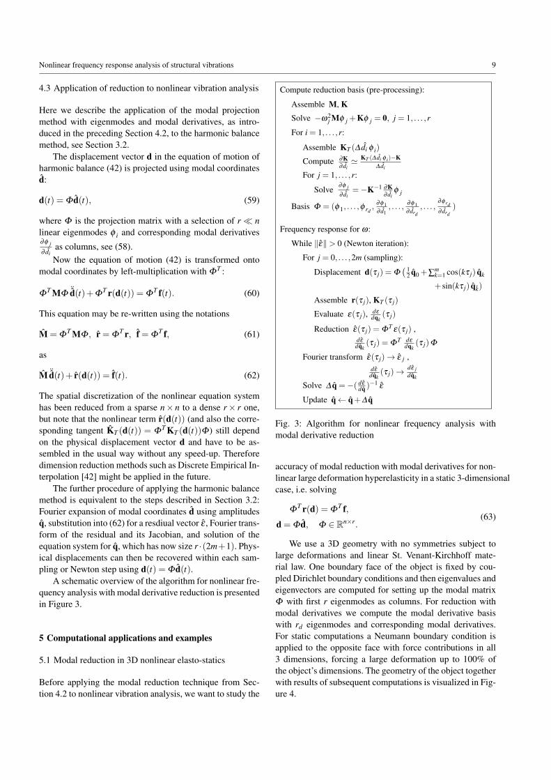
4.3 Application of reduction to nonlinear vibration analysis

Here we describe the application of the modal projectionmethod with eigenmodes and modal derivatives, as intro-duced in the preceding Section 4.2, to the harmonic balancemethod, see Section 3.2.

The displacement vector d in the equation of motion ofharmonic balance (42) is projected using modal coordinatesd:

d(t) = Φ d(t), (59)

where Φ is the projection matrix with a selection of r nlinear eigenmodes φ i and corresponding modal derivatives∂φ j

∂ dias columns, see (58).Now the equation of motion (42) is transformed onto

modal coordinates by left-multiplication with ΦT :

ΦT MΦ

¨d(t)+ΦT r(d(t)) = Φ

T f(t). (60)

This equation may be re-written using the notations

M = ΦT MΦ , r = Φ

T r, f = ΦT f, (61)

as

M ¨d(t)+ r(d(t)) = f(t). (62)

The spatial discretization of the nonlinear equation systemhas been reduced from a sparse n× n to a dense r× r one,but note that the nonlinear term r(d(t)) (and also the corre-sponding tangent KT (d(t)) = Φ

T KT (d(t))Φ) still dependon the physical displacement vector d and have to be as-sembled in the usual way without any speed-up. Thereforedimension reduction methods such as Discrete Empirical In-terpolation [42] might be applied in the future.

The further procedure of applying the harmonic balancemethod is equivalent to the steps described in Section 3.2:Fourier expansion of modal coordinates d using amplitudesq, substitution into (62) for a resdiual vector ε , Fourier trans-form of the residual and its Jacobian, and solution of theequation system for q, which has now size r ·(2m+1). Phys-ical displacements can then be recovered within each sam-pling or Newton step using d(t) = Φ d(t).

A schematic overview of the algorithm for nonlinear fre-quency analysis with modal derivative reduction is presentedin Figure 3.

5 Computational applications and examples

5.1 Modal reduction in 3D nonlinear elasto-statics

Before applying the modal reduction technique from Sec-tion 4.2 to nonlinear vibration analysis, we want to study the

Compute reduction basis (pre-processing):

Assemble M, KSolve −ω2

j Mφ j +Kφ j = 0, j = 1, . . . ,r

For i = 1, . . . ,r:

Assemble KT (∆ di φ i)

Compute ∂K∂ di' KT (∆ di φ i)−K

∆ di

For j = 1, . . . ,r:

Solve∂φ j

∂ di=−K−1 ∂K

∂ diφ j

Basis Φ = (φ 1, . . . ,φ rd,

∂φ1∂ d1

, . . . ,∂φ1∂ drd

, . . . ,∂φ rd∂ drd

)

Frequency response for ω:

While ‖ε‖> 0 (Newton iteration):

For j = 0, . . . ,2m (sampling):

Displacement d(τ j) = Φ( 1

2 q0 +∑mk=1 cos(kτ j) qk

+sin(kτ j) qk)

Assemble r(τ j), KT (τ j)

Evaluate ε(τ j), dε

dqk(τ j)

Reduction ε(τ j) = ΦT

ε(τ j) ,dε

dqk(τ j) = Φ

T dε

dqk(τ j)Φ

Fourier transform ε(τ j)→ ε j ,dε

dqk(τ j)→

dε jdqk

Solve ∆ q =−( dε

dq )−1 ε

Update q← q+∆ q

Fig. 3: Algorithm for nonlinear frequency analysis withmodal derivative reduction

accuracy of modal reduction with modal derivatives for non-linear large deformation hyperelasticity in a static 3-dimensionalcase, i.e. solving

ΦT r(d) = Φ

T f,

d = Φ d, Φ ∈ Rn×r.(63)

We use a 3D geometry with no symmetries subject tolarge deformations and linear St. Venant-Kirchhoff mate-rial law. One boundary face of the object is fixed by cou-pled Dirichlet boundary conditions and then eigenvalues andeigenvectors are computed for setting up the modal matrixΦ with first r eigenmodes as columns. For reduction withmodal derivatives we compute the modal derivative basiswith rd eigenmodes and corresponding modal derivatives.For static computations a Neumann boundary condition isapplied to the opposite face with force contributions in all3 dimensions, forcing a large deformation up to 100% ofthe object’s dimensions. The geometry of the object togetherwith results of subsequent computations is visualized in Fig-ure 4.

10 O. Weeger et al.

Fig. 4 Geometry of the 3D object(grey), linear displacement (blue), non-linear displacement (red), nonlinear dis-placement with modal reduction r = 50(green).

For a quite coarse isogeometric discretization with p =

(2,2,2), ` = (2,2,4), n = (4,4,6), N = 288, we comparethe accuracy of modal reduction (MR) and modal reduc-tion with derivatives (MD) with the full, unreduced nonlin-ear computation. As criteria we use the relative errors of x-,y- and z-displacement, evaluated on the center point of thesurface where the load is applied, e.g. |ufull

x −uMDx |/|ufull

x |,as well as relative errors in L2- and H1-norms, e.g. ‖ufull−uMD‖L2/‖ufull‖L2 .

In Figure 5 we compare the relative L2- and H1-errorsof the full and reduced solutions for the linear case with MRand the nonlinear case with MR and MD. While no signif-icant improvement of accuracy with increasing basis length(number of modes) is noticable for MR in the nonlinear case,MD provides a similar convergence behaviour as MR in thelinear case. Note that for r = 240 we are already consideringthe full set of displacement modes and for r = N the trans-formation is bijective and thus must reproduce the results ofthe full system.

Furthermore we have also investigated the behaviour ofmodal reduction and modal derivatives for different load fac-tors. Figure 6 shows the displacement at the evaluation pointfor load facor 1 to 1000 (100 corresponds to the load levelof previous results). While there is no visible deviation fromfull results for MD, MR shows large errors.

In Figure 7 the relative errors of the displacment at eval-uation point and relative L2- and H1-norm errors are shownover increasing load factor. While errors for MD are smalland roughly stay constant up to very large load factors and

thus displacements, relative errors for MR grow fast and toa very high, unreliable level.

With this numerical study we have examined the ap-proximation properties of our modal reduction method forlarge deformations in a static setting. We can conclude thatmodal reduction is unsuitable for reduction of large defor-mation problems, while modal reduction with modal deriva-tives provides a high accuracy in the nonlinear static prob-lem setting and opens a perspective for the use in nonlinearvibration analysis.

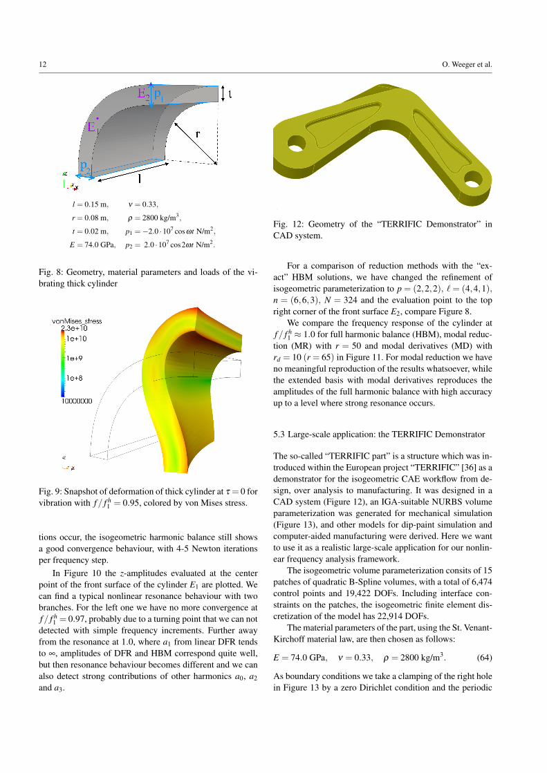
5.2 Large amplitude vibration of a thick cylinder

Mathisen et al. already studied the use of isogeometric anal-ysis in compressible and incompressible hyperelasticity withNeo-Hooke materials [34]. We pick up the example, with ageometry that can be exactly represent using a NURBS vol-ume, with a compressible Neo-Hooke material law for non-linear vibration analysis. The dimensions of on eight of thecylinder, material parameters and loads can be found in Fig-ure 8. The surface Neumann loads are periodic.

For the isogeometric discretization we chose p=(3,3,3),` = (4,4,1), n = (7,7,4), N = 588, and therefore computethe first linear eigenfrequency as f h

1 = 1581.9 Hz.Now we perform a harmonic balance frequency response

analysis with m = 3 (HBM) near the first eigenfrequencywithin the frequency range of 0.85 < f/ f h

1 < 1.15 and com-pare the results with linear direct frequency reponse (DFR).A snapshot of the deformed vibrating cylinder for f/ f h

1 =

0.95 can be seen in Figure 9. Although very large deforma-

Nonlinear frequency response analysis of structural vibrations 11

100 101 102 10310−6

10−5

10−4

10−3

10−2

10−1

100

basis length r

rela

tive

erro

r

linear, MRL2-errorH1-errornonlin., MRL2-errorH1-errornonlin., MDL2-errorH1-error Fig. 5 Convergence of

modal reduction w.r.t. basislength r in relative L2- andH1-norms. Poor results formodal reduction (MR) inthe nonlinear case, whileenhanced basis (MD) fornonlinear problem performsas good as modal basis inlinear case

100 101 102 103−0.10

−0.05

0.00

0.05

0.10

0.15

0.20

0.25

load factor

disp

lace

men

t

fulluxuyuz

MR r = 50uxuyuz

MD rd = 10uxuyuz

Fig. 6 Displacement atevaluation point for fullcomputation (full), modalreduction with 50 modes(MR r = 50) and modalderivatives for 10 modes(MD rd = 10) for increasingload factor

100 101 102 10310−4

10−3

10−2

10−1

100

load factor

rela

tive

erro

r

MR r = 50L2

H1

uxuyuz

MD rd = 10L2

H1

uxuyuz

Fig. 7 Relative error of dis-placement amplitudes, L2-and H1-norm of MR (r =50) and MD (rd = 10) w.r.tfull computation for increas-ing load factor

12 O. Weeger et al.

l = 0.15 m, ν = 0.33,

r = 0.08 m, ρ = 2800 kg/m3,

t = 0.02 m, p1 =−2.0 ·107 cosωt N/m2,

E = 74.0 GPa, p2 = 2.0 ·107 cos2ωt N/m2.

Fig. 8: Geometry, material parameters and loads of the vi-brating thick cylinder

Fig. 9: Snapshot of deformation of thick cylinder at τ = 0 forvibration with f/ f h

1 = 0.95, colored by von Mises stress.

tions occur, the isogeometric harmonic balance still showsa good convergence behaviour, with 4-5 Newton iterationsper frequency step.

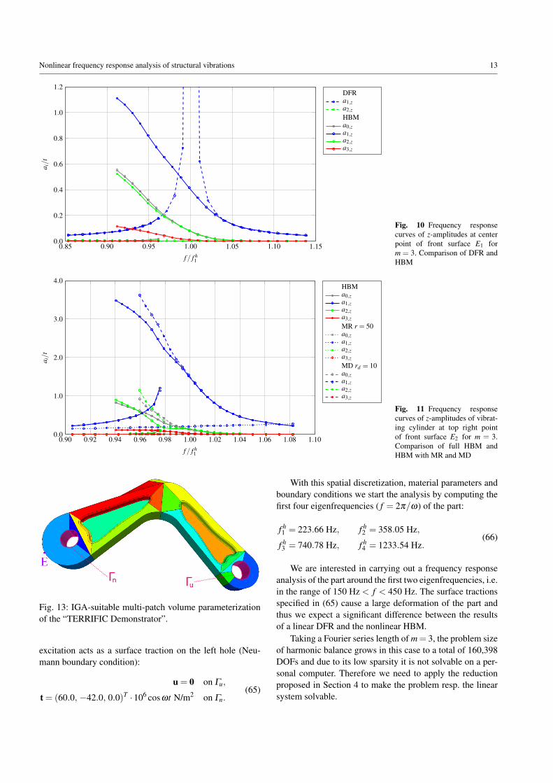
In Figure 10 the z-amplitudes evaluated at the centerpoint of the front surface of the cylinder E1 are plotted. Wecan find a typical nonlinear resonance behaviour with twobranches. For the left one we have no more convergence atf/ f h

1 = 0.97, probably due to a turning point that we can notdetected with simple frequency increments. Further awayfrom the resonance at 1.0, where a1 from linear DFR tendsto ∞, amplitudes of DFR and HBM correspond quite well,but then resonance behaviour becomes different and we canalso detect strong contributions of other harmonics a0, a2and a3.

Fig. 12: Geometry of the “TERRIFIC Demonstrator” inCAD system.

For a comparison of reduction methods with the “ex-act” HBM solutions, we have changed the refinement ofisogeometric parameterization to p = (2,2,2), `= (4,4,1),n = (6,6,3), N = 324 and the evaluation point to the topright corner of the front surface E2, compare Figure 8.

We compare the frequency response of the cylinder atf/ f h

1 ≈ 1.0 for full harmonic balance (HBM), modal reduc-tion (MR) with r = 50 and modal derivatives (MD) withrd = 10 (r = 65) in Figure 11. For modal reduction we haveno meaningful reproduction of the results whatsoever, whilethe extended basis with modal derivatives reproduces theamplitudes of the full harmonic balance with high accuracyup to a level where strong resonance occurs.

5.3 Large-scale application: the TERRIFIC Demonstrator

The so-called “TERRIFIC part” is a structure which was in-troduced within the European project “TERRIFIC” [36] as ademonstrator for the isogeometric CAE workflow from de-sign, over analysis to manufacturing. It was designed in aCAD system (Figure 12), an IGA-suitable NURBS volumeparameterization was generated for mechanical simulation(Figure 13), and other models for dip-paint simulation andcomputer-aided manufacturing were derived. Here we wantto use it as a realistic large-scale application for our nonlin-ear frequency analysis framework.

The isogeometric volume parameterization consits of 15patches of quadratic B-Spline volumes, with a total of 6,474control points and 19,422 DOFs. Including interface con-straints on the patches, the isogeometric finite element dis-cretization of the model has 22,914 DOFs.

The material parameters of the part, using the St. Venant-Kirchoff material law, are then chosen as follows:

E = 74.0 GPa, ν = 0.33, ρ = 2800 kg/m3. (64)

As boundary conditions we take a clamping of the right holein Figure 13 by a zero Dirichlet condition and the periodic

Nonlinear frequency response analysis of structural vibrations 13

0.85 0.90 0.95 1.00 1.05 1.10 1.150.0

0.2

0.4

0.6

0.8

1.0

1.2

f/ f h1

a i/t

DFRa1,za2,z

HBMa0,za1,za2,za3,z

Fig. 10 Frequency responsecurves of z-amplitudes at centerpoint of front surface E1 form = 3. Comparison of DFR andHBM

0.90 0.92 0.94 0.96 0.98 1.00 1.02 1.04 1.06 1.08 1.100.0

1.0

2.0

3.0

4.0

f/ f h1

a i/t

HBMa0,za1,za2,za3,z

MR r = 50a0,za1,za2,za3,z

MD rd = 10a0,za1,za2,za3,z

Fig. 11 Frequency responsecurves of z-amplitudes of vibrat-ing cylinder at top right pointof front surface E2 for m = 3.Comparison of full HBM andHBM with MR and MD

Fig. 13: IGA-suitable multi-patch volume parameterizationof the “TERRIFIC Demonstrator”.

excitation acts as a surface traction on the left hole (Neu-mann boundary condition):

u = 0 on Γu,

t = (60.0, −42.0, 0.0)T ·106 cosωt N/m2 on Γn.(65)

With this spatial discretization, material parameters andboundary conditions we start the analysis by computing thefirst four eigenfrequencies ( f = 2π/ω) of the part:

f h1 = 223.66 Hz, f h

2 = 358.05 Hz,

f h3 = 740.78 Hz, f h

4 = 1233.54 Hz.(66)

We are interested in carrying out a frequency responseanalysis of the part around the first two eigenfrequencies, i.e.in the range of 150 Hz < f < 450 Hz. The surface tractionsspecified in (65) cause a large deformation of the part andthus we expect a significant difference between the resultsof a linear DFR and the nonlinear HBM.

Taking a Fourier series length of m = 3, the problem sizeof harmonic balance grows in this case to a total of 160,398DOFs and due to its low sparsity it is not solvable on a per-sonal computer. Therefore we need to apply the reductionproposed in Section 4 to make the problem resp. the linearsystem solvable.

14 O. Weeger et al.

full rd = 5 rd = 10

abs. val. abs. val. rel. err. abs. val. rel. err.

ux 1.42E-02 1.33E-02 5.7% 1.41E-02 0.04%

uy 6.57E-03 5.85E-03 11.0% 6.59E-03 0.27%

uz 1.05E-03 2.69E-03 155.8% 1.05E-03 0.48%

L2 1.53E-04 1.45E-04 11.8% 1.53E-04 0.24%

H1 1.47E-03 1.40E-03 8.4% 1.47E-03 0.80%

Table 1: Nonlinear static analysis of “TERRIFIC Demon-strator”. Comparison of full problem and reduction withmodal derivatives.

As part of pre-processing we compute the nonlinear staticdisplacement caused by a static load of the same magni-tude. Then we compute the reduction basis with 5 resp. 10linear eigenmodes and all corresponding modal derivatives,and solve the reduced versions of the nonlinear static prob-lem. A comparison of absolute values and relative errorsof displacements at an evaluation point on the very left ofthe structure (which we also take for plotting frequency re-sponse curves), L2- and H1-norms in Table 1 reveals thatrd = 5 is not sufficient to capture the nonlinear displacementbehaviour, whereas rd = 10 provides a sufficient accuracy of‖u f ull−urd‖L2/‖u f ull‖L2 < 1.0%.

We proceed with the harmonic balance frequency re-sponse analysis in conjunction with modal derivative reduc-tion with rd = 10, i.e. the first 10 linear eigenmodes andthe rd(rd + 1)/2 = 55 corresponding modal derivatives. InFigures 14, 15, 16 we have plotted the frequency responsecurves of x-, y- and z-amplitudes evaluated at evaluationpoint E on the left outer boundary of the “TERRIFIC part”for the frequency range 150 Hz < f < 450 Hz, togehter withcorresponding amplitudes computed from linear DFR. Aroundf = 159.0 Hz = f h

2 /2 there is a remarkable sub-harmonicresponse in a2, which can not be determined with linear fre-quency analysis. In the vicinity of the first eigenfrequencyf h1 = 223.7 Hz we notice that the nonlinear response be-

haviour in z-amplitudes is different from the linear one ob-tained from DFR. The resonance behaviour around f h

2 =

358.0 Hz is very strong and we have convergence problemswith our method for 335 Hz < f < 355 Hz. There are strongcontributions from higher harmonics here, which lead to muchmore realistic deformations as we discuss in more detailbelow. Rapidly growing z-amplitudes at resonance indicatethat there might by turning points in the frequency responsecurves here, which we could only follow using continuationmethods.

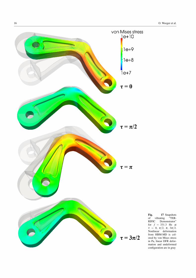
Figure 17 shows the vibrating structure at a frequencyof f = 331.3 Hz, i.e. near the first eigenfrequency of f h

1 =

358.1 Hz, where resonance with very large deformation oc-

curs. Four snapshots are taken at times τ = 0, π/2, π, 3π/2,displaying the deformed structure from the HBM-MD com-putation colored by von Mises stress in Pa and as referencesthe deformed structure from DFR linear frequency analysisand undeformed structure both in gray. It becomes obviousthat the nonlinear results lead to a much better conserva-tion of volume of the structure and thus much more realis-tic states of deformation. Furthermore it is interesting thatthe bending of the structure is stronger in the nonlinear casethan in the linear case for τ = π . This can as well be ob-served in Figure 18, where we have plotted the x-, y- andz-displacement at the evaluation point over one vibration pe-riod of τ ∈ [0,2π] for f = 331.3 Hz for both HBM-MD andDFR.

Altogether, the results we present for the “TERRIFICDemonstrator” show that a modal reduction with modal deriva-tives makes harmonic balance nonlinear frequency responseanalysis feasible even for larger applications.

6 Summary and outlook

The aim of this paper is to present an advanced method fornonlinear frequency response analysis of large-scale appli-cations in solid mechanics.

We have proposed to use the harmonic balance methodfor nonlinear steady-state frequency response of the discretizedequation of motion in the frequency domain. In conjunctionwith a modal projection method using eigenmodes and sec-ond order modal derivatives as reduction basis, the methodcan be applied even to realistic applications with large spa-tial discretizations. For an efficient spatial discretization ofthe nonlinear partial differential equations arising from 3-dimensional large deformation hyperelasticity we employthe isogeometric finite element method, but our approachcould be applied using any spatial discretization method.As our numerical examples show, the reduction method pro-vides a good accuracy of frequency response amplitudes andresonance behaviour, although significantly reduces the ef-fort for numerical solution of the harmonic balance equa-tion system. For large-scale applications harmonic balancebecomes feasible only using model order reduction.

Even though the proposed reduction method makes non-linear frequency response analysis feasible in application to3-dimensional structural problems, it still remains a time-consuming task. Especially for very large applications a speed-up of the sampling process is necessary, where full residualand tangent stiffness have to be assembled for every sample.A complexity reduction might there be achieved by methodssuch as Discrete Empirical Interpolation [42]. For furtherindustrial problems we plan to extend the method to mate-rials with nonlinear viscoelastic properties such as rubberand contact problems. We also aim at combining nonlinearfrequency analysis with shape optimization.

Nonlinear frequency response analysis of structural vibrations 15

150 200 250 300 350 400 450−0.15

−0.10

−0.05

0.00

0.05

0.10

0.15

f [Hz]

a i,x

[m]

DFRa1,x

HBMa0,xa1,xa2,xa3,x

Fig. 14 Frequency responsecurves of x-amplitudesof vibrating “TERRIFICDemonstrator” for DFR andHBM with reduction

150 200 250 300 350 400 450−0.10

−0.05

0.00

0.05

0.10

f [Hz]

a i,y

[m]

DFRa1,y

HBMa0,ya1,ya2,ya3,y

Fig. 15 Frequency responsecurves of y-amplitudesof vibrating “TERRIFICDemonstrator” for DFR andHBM with reduction

150 200 250 300 350 400 450−4.00

−2.00

0.00

2.00

4.00·10−2

f [Hz]

a i,z

[m]

DFRa1,z

HBMa0,za1,za2,za3,z

Fig. 16 Frequency responsecurves of z-amplitudesof vibrating “TERRIFICDemonstrator” for DFR andHBM with reduction

16 O. Weeger et al.

Fig. 17 Snapshotsof vibrating “TER-RIFIC Demonstrator”for f = 331.3 Hz atτ = 0, π/2, π, 3π/2.Nonlinear deformationfrom HBM-MD is col-ored by von Mises stressin Pa, linear DFR defor-mation and undeformedconfiguration are in gray

Nonlinear frequency response analysis of structural vibrations 17

0 12 π

π 32 π 2π

−0.10

−0.05

0.00

0.05

0.10

τ = 2π f t

u i[m

]

DFRuxuyuz

HBMuxuyuz

Fig. 18 Displacementof evaluation point on“TERRIFIC Demonstra-tor” for f = 331.3 Hz forHBM-MD and DFR

Acknowledgements This work is supported by the European Unionwithin the FP7-project TERRIFIC: Towards Enhanced Integration ofDesign and Production in the Factory of the Future through Isogeo-metric Technologies [36].

The “TERRIFIC part” was designed by Stefan Boschert (SiemensAG, Germany) and the isogeometric parameterization provided by Vi-beke Skytt (SINTEF, Norway).

References

1. A.H. Nayfeh and B. Balachandran. Applied Nonlinear Dynam-ics: Analytical Computational, and Experimental Methods. WileySeries in Nonlinear Science. John Wiley & Sons, 1995.

2. A.H. Nayfeh and D.T. Mook. Nonlinear Oscillations. Wiley Clas-sics Library. John Wiley & Sons, 1995.

3. W. Szemplinska-Stupnicka. The Behaviour of Nonlinear VibratingSystems. Kluwer Academic Publishers, Dordrecht Boston Lon-don, 1990.

4. O. Weeger, U. Wever, and B. Simeon. Isogeometric analysis ofnonlinear euler-bernoulli beam vibrations. Nonlinear Dynamics,72(4):813–835, 2013.

5. P. Wriggers. Nonlinear Finite Element Methods. Springer, 2008.6. T. Belytschko, W. K. Liu, and B. Moran. Nonlinear Finite Ele-

ments for Continua and Structures. John Wiley & Sons, 2000.7. Cadence Design Systems Inc. Rf analysis in virtuoso spectre cir-

cuit simulator xl datasheet. Technical report, 2007.8. M. Schneider, U. Wever, and Q. Zheng. Parallel harmonic balance.

VLSI 93, Proceedings of the IFIP TC10/WG 10.5 InternationalConference on Very Large Scale Integration, Grenoble, France,7-10 September, 1993, pages 251–260, 1993.

9. R. Lewandowski. Non-linear, steady-state vibration of structuresby harmonic balance/finite element method. Computers & Struc-tures, 44(1-2):287–296, 1992.

10. R. Lewandowski. Computational formulation for periodic vi-bration of geometrically nonlinear structures, part 1: Theoreticalbackground; part 2: Numerical strategy and examples. Interna-tional Journal of Solids and Structures, 34(15):1925–1964, 1997.

11. P. Ribeiro and M. Petyt. Non-linear vibration of beams with inter-nal resonance by the hierarchical finite element method. Journalof Sound and Vibration, 224(15):591–624, 1999.

12. P. Ribeiro. Hierarchical finite element analyses of geometricallynon-linear vibration of beams and plane frames. Journal of Soundand Vibration, 246(2):225–244, 2001.

13. P. Ribeiro. Non-linear forced vibrations of thin/thick beams andplates by the finite element and shooting methods. Computers andStructures, 82(17-19):1413–1423, 2004.

14. T.J.R. Hughes. The Finite Element Method: Linear Static and Dy-namic Finite Element Analysis. Dover Publications, Mineola, NewYork, 2000.

15. Z.-Q. Qu. Model Order Reduction Techniques with Applicationsin Finite Element Analysis. Springer, 2004.

16. Malte Krack, Lars Panning von Scheidt, and Jorg Wallaschek. Amethod for nonlinear modal analysis and synthesis: Application toharmonically forced and self-excited mechanical systems. Journalof Sound and Vibration, 332(25):6798–6814, 2013.

17. S. R. Idelsohn and A. Cardona. A reduction method for nonlin-ear structural dynamics analysis. Comput. Methods Appl. Mech.Engrg., 49:253–279, 1985.

18. P. M. A. Slaats, J. de Jongh, and A. A. H. J. Sauren. Model reduc-tion tools for nonlinear structural dynamics. Computers & Struc-tures, 54(6):1155–1171, 1995.

19. J. Barbic. Real-time Reduced Large-Deformation Models and Dis-tributed Contact for Computer Graphics and Haptics. PhD thesis,Carnegie Mellon University, 2007.

20. J. Barbic. Fem simulation of 3d deformable solids: A practi-tioner‘s guide to theory, discretization and model reduction. part2: Model reduction. In SIGGRAPH 2012 Course Notes, 2012.

21. H. Spiess. Reduction Methods in Finite Element Analysis of Non-linear Structural Dynamics. PhD thesis, Universitat Hannover,2005.

22. J. Remke and H. Rothert. Eine modale reduktionsmethodezur geometrisch nichtlinearen statischen und dynamischen finite-element-berechnung. Archive of Applied Mechanics, 63(2):101 –115, 1993.

23. Oleg Roderick, Mihai Anitescu, and Paul Fischer. Polynomial re-gression approaches using derivative information for uncertaintyquantification. Nuclear Science and Engineerin, 164(2):122–139,2010.

24. T.J.R. Hughes, J.A. Cottrell, and Y. Bazilevs. Isogeometric anal-ysis: Cad, finite elements, nurbs, exact geometry and mesh refine-ment. Computer Methods in Applied Mechanics and Engineering,194(39–41):4135–4195, 2005.

25. L.A. Piegl and W. Tiller. The Nurbs Book. Monographs in VisualCommunication. Springer, 1997.

26. R.N. Simpson, S.P.A. Bordas, J. Trevelyan, and T. Rabczuk. Atwo-dimensional isogeometric boundary element method for elas-tostatic analysis. Computer Methods in Applied Mechanics andEngineering, 209-212:87–100, 2012.

27. F. Auricchio, L. Beirao da Veiga, T.J.R. Hughes, A. Reali, andG. Sangalli. Isogeometric collocation methods. Mathemati-cal Models and Methods in Applied Sciences, 20(11):2075–2107,2010.

28. Ch. Heinrich, B. Simeon, and S. Boschert. A finite volumemethod on nurbs geometries and its application in isogeometricfluid–structure interaction. Mathematics and Computers in Simu-lation, 82(9):1645–1666, 2012.

18 O. Weeger et al.

29. J.A. Cottrell, T.J.R. Hughes, and Y. Bazilevs. Isogeometric Anal-ysis: Toward Integration of CAD and FEA. John Wiley & Sons,Ltd, 2009.

30. J.A. Cottrell, A. Reali, Y. Bazilevs, and T.J.R. Hughes. Isogeomet-ric analysis of structural vibrations. Computer Methods in AppliedMechanics and Engineering, 195(41–43):5257–5296, 2006.

31. T.J.R. Hughes, J.A. Evans, and A. Reali. Finite element and nurbsapproximations of eigenvalue, boundary-value, and initial-valueproblems. Computer Methods in Applied Mechanics and Engi-neering, 272:290–320, 2014.

32. T. Elguedj, Y. Bazilevs, V. M. Calo, and T. J. R. Hughes. B-barand f-bar projection methods for nearly incompressible linear andnon-linear elasticity and plasticity based on higher-order nurbs el-ements. Computer Methods in Applied Mechanics and Engineer-ing, 197:2732–2762, 2008.

33. F. Auricchio, L. Beirao da Veiga, C. Lovadina, and A. Reali. Theimportance of the exact satisfaction of the incompressibility con-straint in nonlinear elasticity: mixed fems versus nurbs-based ap-proximations. Computer Methods in Applied Mechanics and En-gineering, 199:314–323, 2010.

34. K. M. Mathisen, K. M. Okstad, T. Kvamsdal, and S. B. Raknes.Isogeometric analysis of finite deformation nearly incompressiblesolids. Rakenteiden Mekaniikka (Journal of Structural Mechan-ics), 44(3):260–278, 2011.

35. R. Kolman. Isogeometric free vibration of an elastic block. Engi-neering Mechanics, 19(4):279–291, 2012.

36. Terrific project, October 2011.37. C. Touze and M. Amabili. Nonlinear normal modes for damped

geometrically nonlinear systems: Application to reduced-ordermodelling of harmonically forced structures. Journal of Soundand Vibration, 298:958–981, 2006.

38. C. Touze, M. Amabili, and O. Thomas. Reduced-order modelsfor large-amplitude vibrations of shells including in-plane inertia.Comput. Methods Appl. Mech. Engrg., 197:2030–2045, 2008.

39. Polarit Apiwattanalunggarn, Steven W. Shaw, Christophe Pierre,and Dongying Jiang. Finite-element-based nonlinear modal re-duction of a rotating beam with large-amplitude motion. Journalof Vibration and Control, 9:235–263, 2003.

40. U. Becker. Efficient time integration and nonlinear model reduc-tion for incompressible hyperelastic materials. PhD thesis, TUKaiserslautern, 2012.

41. S. Herkt. Model Reduction of Nonlinear Problems in StructuralMechanics: Towards a Finite Element Tyre Model for MultibodySimulation. PhD thesis, TU Kaiserslautern, 2008.

42. S. Chaturantabut and D.C. Sorensen. Nonlinear model reduc-tion via discrete empirical interpolation. SIAM J. Sci. Comput.,32(5):2737–2764, 2010.