nonlinear programming: concepts and algorithms for...
TRANSCRIPT
1
Nonlinear Programming: Concepts and Algorithms for
Process Optimization
L. T. Biegler Chemical Engineering Department
Carnegie Mellon University Pittsburgh, PA
2
Introduction Unconstrained Optimization • Algorithms • Newton Methods • Quasi-Newton Methods Constrained Optimization • Karush Kuhn-Tucker Conditions • Reduced Gradient Methods (GRG2, CONOPT, MINOS) • Successive Quadratic Programming (SQP) • Interior Point Methods (IPOPT) Process Optimization • Black Box Optimization • Modular Flowsheet Optimization – Infeasible Path • The Role of Exact Derivatives Large-Scale Nonlinear Programming • rSQP: Process Optimization • IPOPT: Blending and Data Reconciliation Summary and Conclusions
Nonlinear Programming and Process Optimization
2
3
Introduction Optimization: given a system or process, find the best solution to this process within constraints.
Objective Function: indicator of "goodness" of solution, e.g., cost, yield, profit, etc.
Decision Variables: variables that influence process behavior and can be adjusted for optimization.
In many cases, this task is done by trial and error (through case study). Here, we are interested in a systematic approach to this task - and to make this task as efficient as possible.
Some related areas:
- Math programming
- Operations Research
Currently - Over 30 journals devoted to optimization with roughly 200 papers/month - a fast moving field!
4
Optimization Viewpoints
Mathematician - characterization of theoretical properties of optimization, convergence, existence, local convergence rates.
Numerical Analyst - implementation of optimization method for efficient and "practical" use. Concerned with ease of computations, numerical stability, performance.
Engineer - applies optimization method to real problems. Concerned with reliability, robustness, efficiency, diagnosis, and recovery from failure.
3
5
Optimization Literature Engineering
1. Edgar, T.F., D.M. Himmelblau, and L. S. Lasdon, Optimization of Chemical Processes, McGraw-Hill, 2001.
2. Papalambros, P. and D. Wilde, Principles of Optimal Design. Cambridge Press, 1988.
3. Reklaitis, G., A. Ravindran, and K. Ragsdell, Engineering Optimization, Wiley, 1983.
4. Biegler, L. T., I. E. Grossmann and A. Westerberg, Systematic Methods of Chemical Process Design, Prentice Hall, 1997.
5. Biegler, L. T., Nonlinear Programming: Concepts, Algorithms and Applications to Chemical Engineering, SIAM, 2010.
Numerical Analysis
1. Dennis, J.E. and R. Schnabel, Numerical Methods of Unconstrained Optimization, Prentice-Hall, (1983), SIAM (1995)
2. Fletcher, R. Practical Methods of Optimization, Wiley, 1987.
3. Gill, P.E, W. Murray and M. Wright, Practical Optimization, Academic Press, 1981.
4. Nocedal, J. and S. Wright, Numerical Optimization, Springer, 2007
6
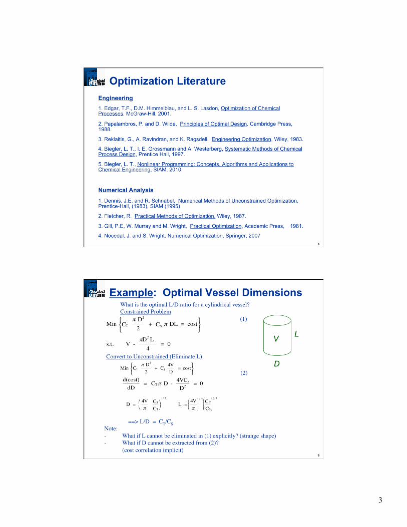
Example: Optimal Vessel Dimensions
Min TC
2! D
2 +
S C ! DL = cost" # $
% & '
s.t. V -
2!D L
4 = 0
Min TC
2! D
2 + S C
4V
D = cost
" # $
% & '
d(cost)
dD = TC ! D -
s4VC2
D = 0
D = 4V
!
SC
TC
" #
$ %
1/ 3
L =4V
!
"
#
& & &
$
%
' ' '
1/3
TC
SC
"
#
& & & &
$
%
' ' ' '
2/3
What is the optimal L/D ratio for a cylindrical vessel?
Constrained Problem
(1)
Convert to Unconstrained (Eliminate L)
(2)
==> L/D = CT/CS
Note:
- What if L cannot be eliminated in (1) explicitly? (strange shape)
- What if D cannot be extracted from (2)? (cost correlation implicit)
L
D
V
4
7
Unconstrained Multivariable Optimization
Problem: Min f(x) (n variables) Equivalent to: Max -f(x), x ∈ Rn Nonsmooth Functions - Direct Search Methods - Statistical/Random Methods Smooth Functions - 1st Order Methods - Newton Type Methods - Conjugate Gradients
8
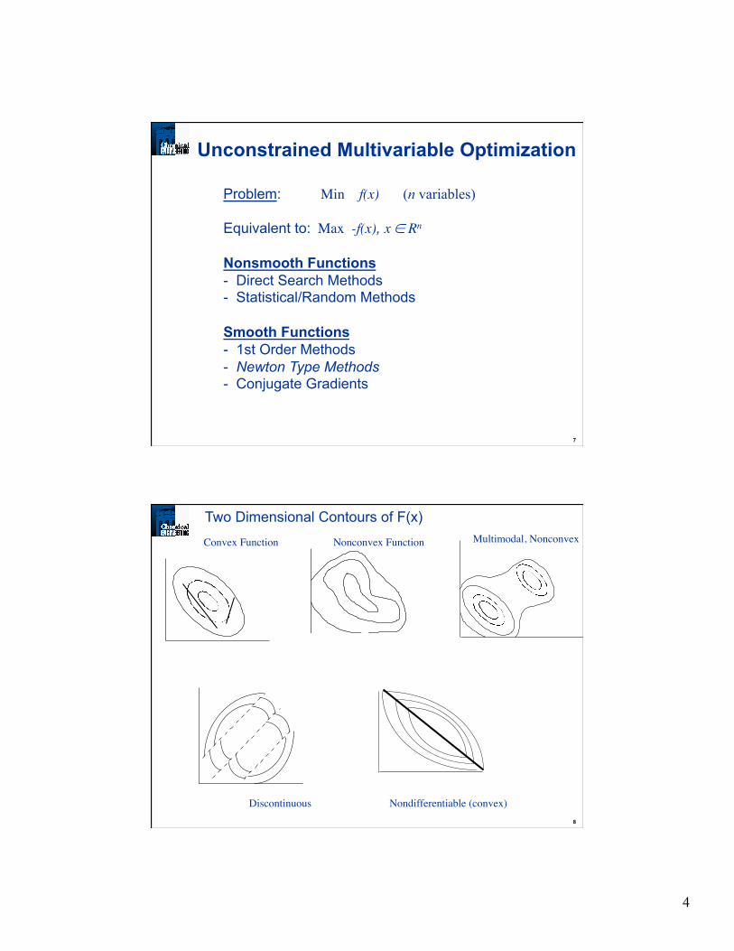
Two Dimensional Contours of F(x)
Convex Function Nonconvex Function Multimodal, Nonconvex
Discontinuous Nondifferentiable (convex)
�
5
9
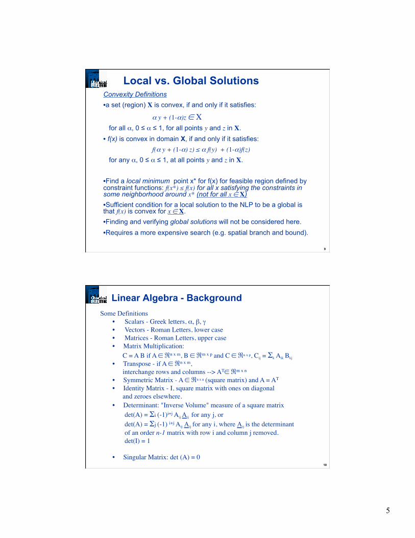
Local vs. Global Solutions Convexity Definitions • a set (region) X is convex, if and only if it satisfies:
α y + (1-α)z ∈ X for all α, 0 ≤ α ≤ 1, for all points y and z in X. • f(x) is convex in domain X, if and only if it satisfies:
f(α y + (1-α) z) ≤ α f(y) + (1-α)f(z) for any α, 0 ≤ α ≤ 1, at all points y and z in X. • Find a local minimum point x* for f(x) for feasible region defined by constraint functions: f(x*) ≤ f(x) for all x satisfying the constraints in some neighborhood around x* (not for all x ∈ X) • Sufficient condition for a local solution to the NLP to be a global is that f(x) is convex for x ∈ X. • Finding and verifying global solutions will not be considered here. • Requires a more expensive search (e.g. spatial branch and bound).
10
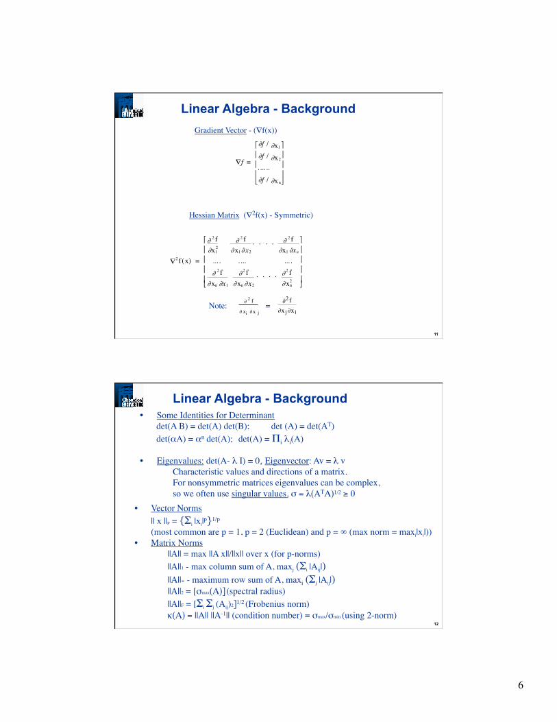
Linear Algebra - Background Some Definitions
• Scalars - Greek letters, α, β, γ • Vectors - Roman Letters, lower case • Matrices - Roman Letters, upper case • Matrix Multiplication: C = A B if A ∈ ℜn x m, B ∈ ℜm x p and C ∈ ℜn x p, Cij = Σk Aik Bkj • Transpose - if A ∈ ℜn x m, interchange rows and columns --> AT∈ ℜm x n
• Symmetric Matrix - A ∈ ℜn x n (square matrix) and A = AT
• Identity Matrix - I, square matrix with ones on diagonal and zeroes elsewhere. • Determinant: "Inverse Volume" measure of a square matrix
det(A) = Σi (-1)i+j Aij Aij for any j, or det(A) = Σj (-1) i+j Aij Aij for any i, where Aij is the determinant of an order n-1 matrix with row i and column j removed. det(I) = 1
• Singular Matrix: det (A) = 0
6
11
!f =
"f /1"x
"f /2"x
.... ..
"f /n"x
#
$
%
%
%
&
'
(
(
(
2! f(x) =
2" f
12"x
2" f
1"x 2"x# # # #
2" f
1"x n"x
... . . ... ... .
2" f
n"x 1"x
2" f
n"x 2"x# # # #
2" f
n2"x
$
%
&
&
&
&
'
(
)
)
)
)
2∂ f
∂ x j∂xi
2! f
j!x i!x
Gradient Vector - (∇f(x))
Hessian Matrix (∇2f(x) - Symmetric)
Note: =
Linear Algebra - Background
12
• Some Identities for Determinant det(A B) = det(A) det(B); det (A) = det(AT) det(αA) = αn det(A); det(A) = Πi λi(A)
• Eigenvalues: det(A- λ I) = 0, Eigenvector: Av = λ v
Characteristic values and directions of a matrix. For nonsymmetric matrices eigenvalues can be complex, so we often use singular values, σ = λ(ATΑ)1/2 ≥ 0
• Vector Norms || x ||p = {Σi |xi|p}1/p (most common are p = 1, p = 2 (Euclidean) and p = ∞ (max norm = maxi|xi|))
• Matrix Norms ||A|| = max ||A x||/||x|| over x (for p-norms) ||A||1 - max column sum of A, maxj (Σi |Aij|) ||A||∞ - maximum row sum of A, maxi (Σj |Aij|) ||A||2 = [σmax(Α)] (spectral radius) ||A||F = [Σi Σj (Aij)2]1/2
(Frobenius norm) κ(Α) = ||A|| ||A-1|| (condition number) = σmax/σmin (using 2-norm)
Linear Algebra - Background
7
13
Find v and λ where Avi = λi vi, i = i,n
Note: Av - λv = (A - λI) v = 0 or det (A - λI) = 0
For this relation λ is an eigenvalue and v is an eigenvector of A. If A is symmetric, all λi are real λi > 0, i = 1, n; A is positive definite
λi < 0, i = 1, n; A is negative definite
λi = 0, some i: A is singular
Quadratic Form can be expressed in Canonical Form (Eigenvalue/Eigenvector)
xTAx ⇒ A V = V Λ
V - eigenvector matrix (n x n)
Λ - eigenvalue (diagonal) matrix = diag(λi)
If A is symmetric, all λi are real and V can be chosen orthonormal (V-1 = VT). Thus, A = V Λ V-1 = V Λ VT
For Quadratic Function: Q(x) = aTx + ½ xTAx
Define: z = VTx and Q(Vz) = (aTV) z + ½ zT (VTAV)z = (aTV) z + ½ zT Λ z Minimum occurs at (if λi > 0) x = -A-1a or x = Vz = -V(Λ-1VTa)
Linear Algebra - Eigenvalues
14
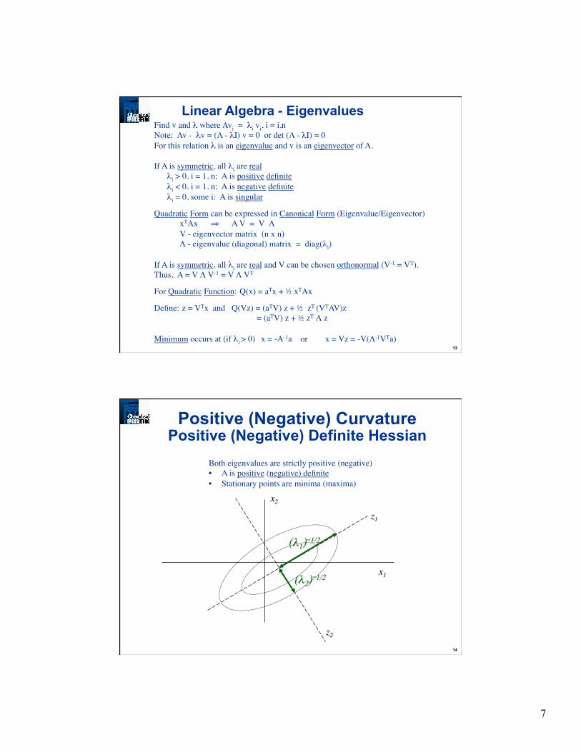
Positive (Negative) Curvature Positive (Negative) Definite Hessian
Both eigenvalues are strictly positive (negative)
• A is positive (negative) definite
• Stationary points are minima (maxima)
x1
x2 z1
z2
(λ1)-1/2
(λ2)-1/2
8
15
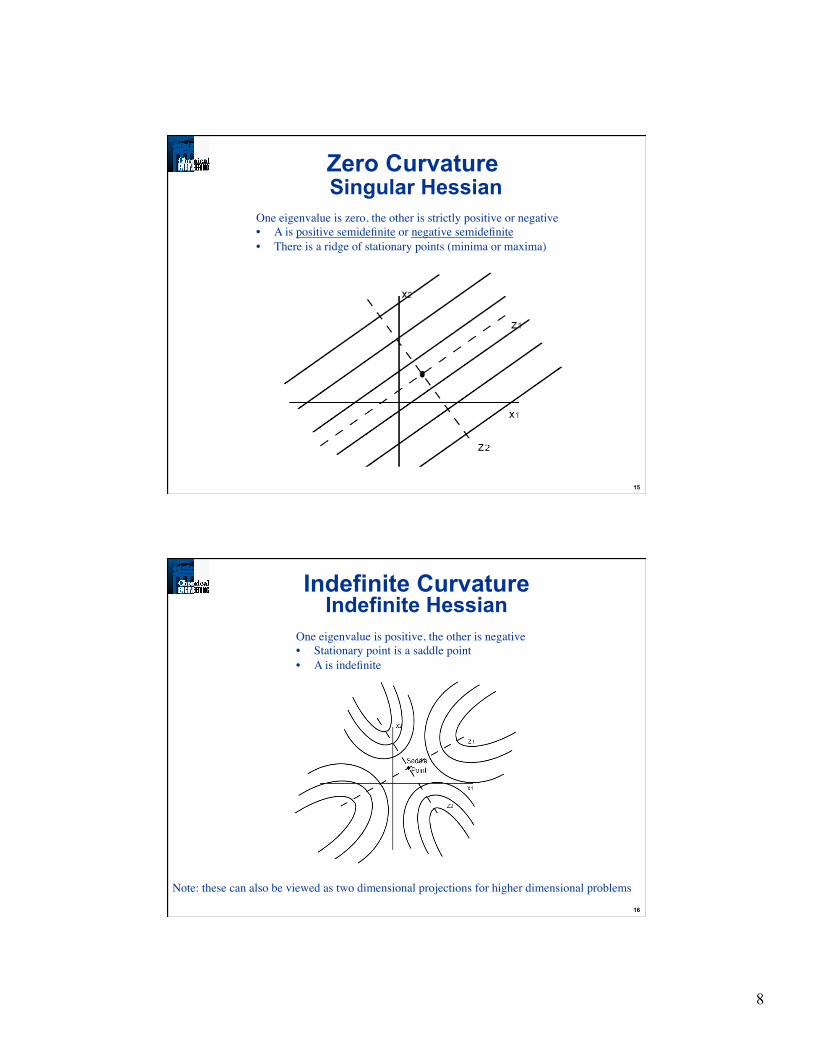
Zero Curvature Singular Hessian
One eigenvalue is zero, the other is strictly positive or negative
• A is positive semidefinite or negative semidefinite
• There is a ridge of stationary points (minima or maxima)
16
One eigenvalue is positive, the other is negative
• Stationary point is a saddle point
• A is indefinite
Note: these can also be viewed as two dimensional projections for higher dimensional problems
Indefinite Curvature Indefinite Hessian
9
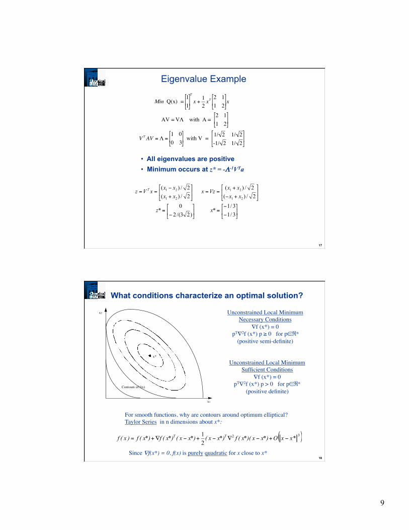
17
Eigenvalue Example
!
!
Min Q(x) =1
1
"
# $ %
& '
T
x +1
2xT
2 1
1 2
"
# $
%
& ' x
AV = V( with A = 2 1
1 2
"
# $
%
& '
VTAV = ( =
1 0
0 3
"
# $
%
& ' with V =
1/ 2 1/ 2
-1/ 2 1/ 2
"
# $
%
& '
• All eigenvalues are positive • Minimum occurs at z* = -Λ-1VTa
−
−=
−=
+−
+==
+
−==
3/13/1
* )23/(2
0*
2/)(2/)(
2/)(2/)(
21
21
21
21
xz
xxxxVzx
xxxxxVz T
18
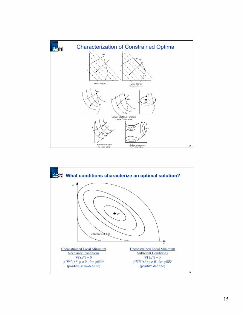
What conditions characterize an optimal solution?
x1
x2
x*
Contours of f(x)
Unconstrained Local Minimum Necessary Conditions
∇f (x*) = 0
pT∇2f (x*) p ≥ 0 for p∈ℜn
(positive semi-definite)
Unconstrained Local Minimum Sufficient Conditions
∇f (x*) = 0
pT∇2f (x*) p > 0 for p∈ℜn
(positive definite)
Since ∇f(x*) = 0, f(x) is purely quadratic for x close to x*
( )32
21 *xxO*)xx*)(x(f*)xx(*)xx(*)x(f*)x(f)x(f TT −+−∇−+−∇+=
For smooth functions, why are contours around optimum elliptical? Taylor Series in n dimensions about x*:
10
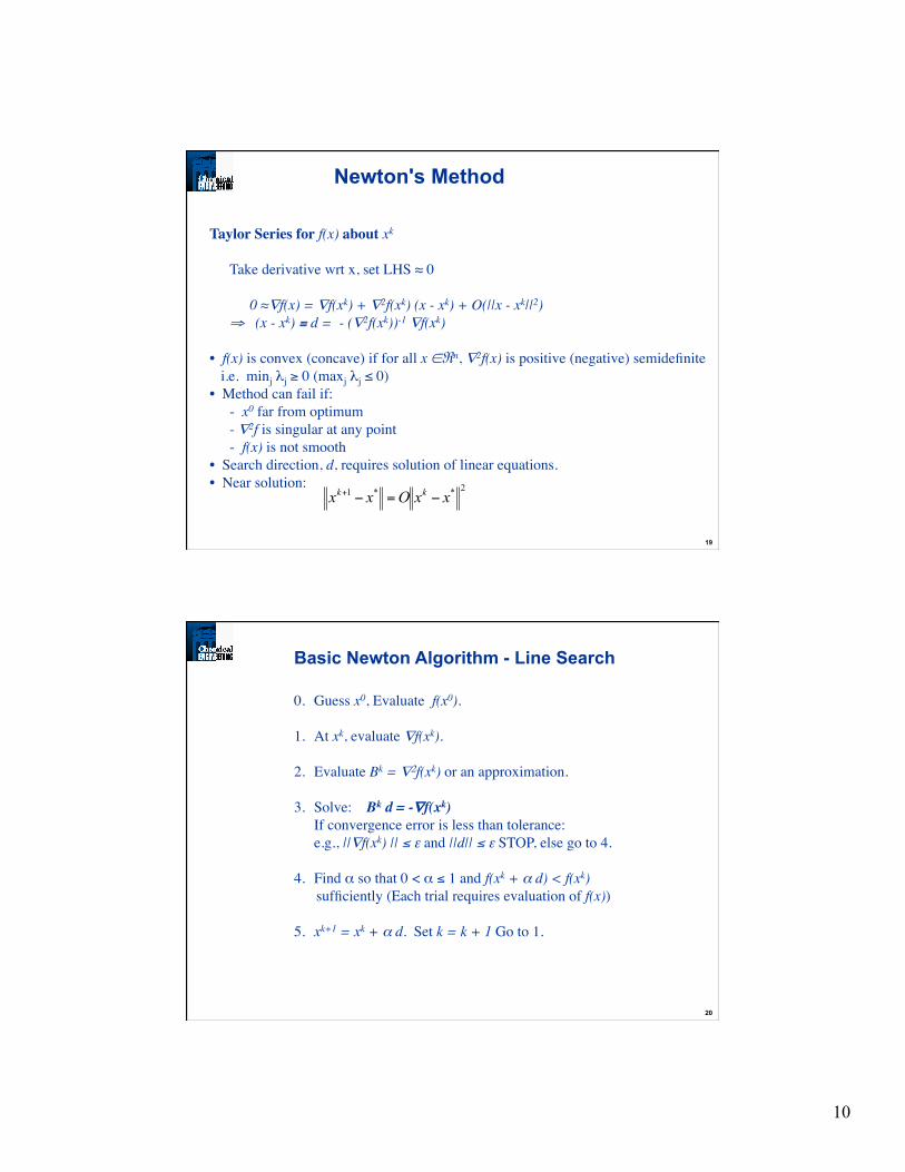
19
Taylor Series for f(x) about xk Take derivative wrt x, set LHS ≈ 0
0 ≈∇f(x) = ∇f(xk) + ∇2f(xk) (x - xk) + O(||x - xk||2) ⇒ (x - xk) ≡ d = - (∇2f(xk))-1 ∇f(xk)
• f(x) is convex (concave) if for all x ∈ℜn, ∇2f(x) is positive (negative) semidefinite i.e. minj λj ≥ 0 (maxj λj ≤ 0) • Method can fail if: - x0 far from optimum - ∇2f is singular at any point - f(x) is not smooth
• Search direction, d, requires solution of linear equations. • Near solution:
�
Newton's Method
2**1 xxOxx kk −=−+
20
0. Guess x0, Evaluate f(x0). 1. At xk, evaluate ∇f(xk). 2. Evaluate Bk = ∇2f(xk) or an approximation. 3. Solve: Bk d = -∇f(xk) If convergence error is less than tolerance: e.g., ||∇f(xk) || ≤ ε and ||d|| ≤ ε STOP, else go to 4.
4. Find α so that 0 < α ≤ 1 and f(xk + α d) < f(xk) sufficiently (Each trial requires evaluation of f(x)) 5. xk+1 = xk + α d. Set k = k + 1 Go to 1. �
Basic Newton Algorithm - Line Search
11
21
1. Convergence Theory
• Global Convergence - will it converge to a local optimum (or stationary point) from a poor starting point?
• Local Convergence Rate - how fast will it converge close to this point?
2. Benchmarks on Large Class of Test Problems
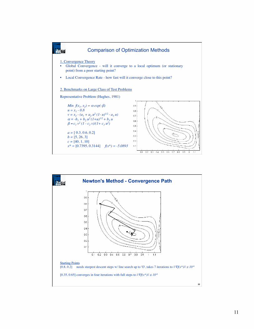
Representative Problem (Hughes, 1981)
Min f(x1, x2) = α exp(-β) u = x1 - 0.8 v = x2 - (a1 + a2 u2 (1- u)1/2 - a3 u) α = -b1 + b2 u2 (1+u)1/2 + b3 u β = c1 v2 (1 - c2 v)/(1+ c3 u2) a = [ 0.3, 0.6, 0.2] b = [5, 26, 3] c = [40, 1, 10] x* = [0.7395, 0.3144] f(x*) = -5.0893
�
Comparison of Optimization Methods
22
Newton's Method - Convergence Path
Starting Points [0.8, 0.2] needs steepest descent steps w/ line search up to 'O', takes 7 iterations to ||∇f(x*)|| ≤ 10-6
[0.35, 0.65] converges in four iterations with full steps to ||∇f(x*)|| ≤ 10-6

12
23
• Choice of Bk determines method. - Steepest Descent: Bk = γ I - Newton: Bk = ∇2f(x)
• With suitable Bk, performance may be good enough if f(xk + αd) is sufficiently decreased (instead of minimized along line search direction). • Trust region extensions to Newton's method provide very strong global convergence properties and very reliable algorithms. • Local rate of convergence depends on choice of Bk.
Newton’s Method - Notes
!
Newton"Quadratic Rate : limk#$
xk+1" x *
xk" x *
2= K
Steepest descent " Linear Rate : limk#$
xk+1" x *
xk" x *
<1
Desired?" Superlinear Rate : limk#$
xk+1" x *
xk" x *
= 0
24
!
k+1
B = k
B + y -
kB s( ) T
y + y y - k
B s( )T
Ty s
- y -
kB s( )
T
s y Ty
Ty s( ) T
y s( )
!
k+1
Bk+1( )
-1
= H = k
H +
TssTs y
-
kH y
Ty kH
ky H y
Motivation: • Need Bk to be positive definite. • Avoid calculation of ∇ 2f. • Avoid solution of linear system for d = - (Bk)-1 ∇f(xk) Strategy: Define matrix updating formulas that give (Bk) symmetric, positive definite and satisfy: (Bk+1)(xk+1 - xk) = (∇f k+1 – ∇f k) (Secant relation)
DFP Formula: (Davidon, Fletcher, Powell, 1958, 1964)
where: s = xk+1- xk y = ∇f (xk+1) - ∇f (xk)
Quasi-Newton Methods
13
25
!
k+1
B = k
B +
TyyTs y
-
kB s T
sk
Bk
s B s
!
k+1
B( )"1
= k+1
H = k
H + s -
kH y( ) T
s + s s - k
H y( )T
Ty s
- y -
kH s( )
T
y s Ts
Ty s( ) T
y s( )
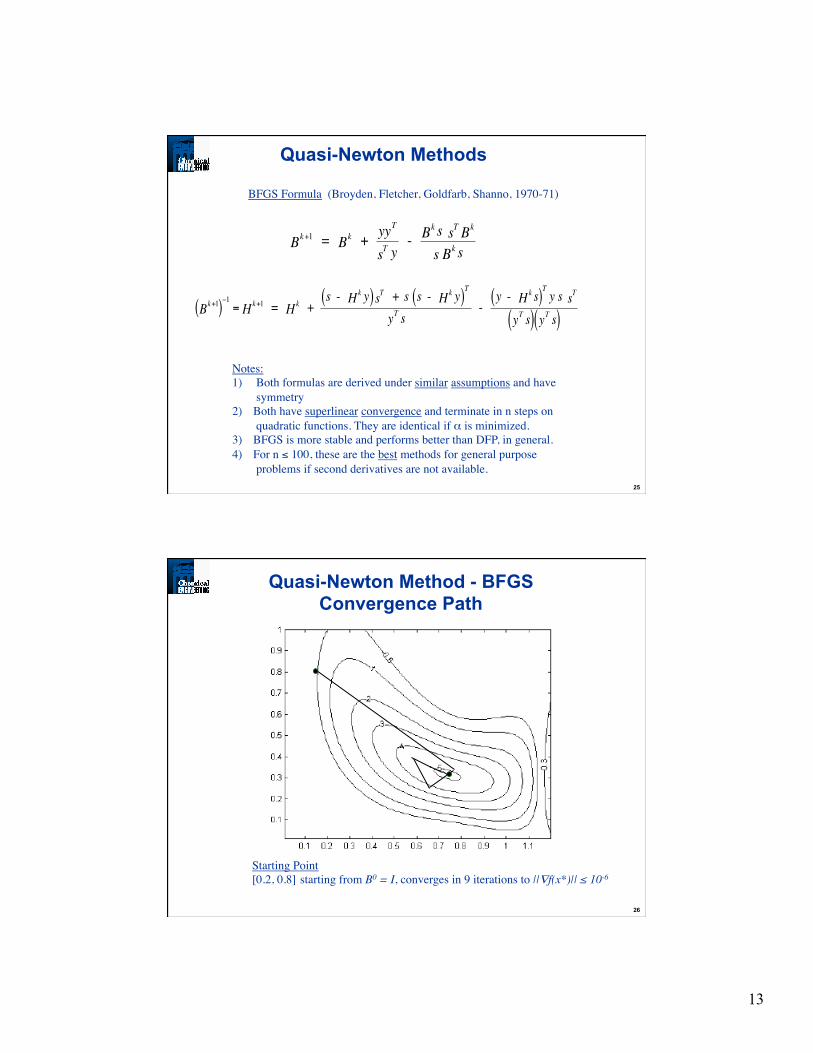
BFGS Formula (Broyden, Fletcher, Goldfarb, Shanno, 1970-71)
Notes:
1) Both formulas are derived under similar assumptions and have symmetry
2) Both have superlinear convergence and terminate in n steps on quadratic functions. They are identical if α is minimized.
3) BFGS is more stable and performs better than DFP, in general. 4) For n ≤ 100, these are the best methods for general purpose
problems if second derivatives are not available.
Quasi-Newton Methods
26
Quasi-Newton Method - BFGS
Convergence Path
Starting Point [0.2, 0.8] starting from B0 = I, converges in 9 iterations to ||∇f(x*)|| ≤ 10-6 �
14
27
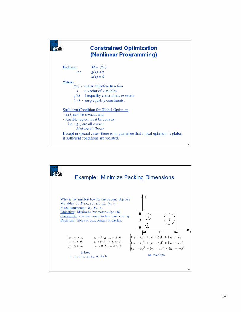
Problem: Minx f(x) s.t. g(x) ≤ 0 h(x) = 0
where: f(x) - scalar objective function x - n vector of variables g(x) - inequality constraints, m vector h(x) - meq equality constraints.
Sufficient Condition for Global Optimum - f(x) must be convex, and - feasible region must be convex, i.e. g(x) are all convex h(x) are all linear
Except in special cases, there is no guarantee that a local optimum is global if sufficient conditions are violated.
Constrained Optimization (Nonlinear Programming)
28
23
1
A
B
y
x
!
1x , 1y " 1R 1x # B - 1R ,
1y # A - 1R
x2,
2 y " 2R 2x # B - 2R ,
2 y # A - 2R
3,x 3 y " 3R 3x # B - 3R ,
3 y # A - 3R
$
% &
' &
!
1x - 2x( )2
+ 1y -
2y( )
2
" 1R + 2R( )2
1x - 3x( )2
+ 1y -
3y( )
2
" 1R + 3R( )2
2x - 3x( )2
+ 2y -
3y( )
2
" 2R + 3R( )2
#
$
% %
&
% %
Example: Minimize Packing Dimensions
What is the smallest box for three round objects?
Variables: A, B, (x1, y1), (x2, y2), (x3, y3)
Fixed Parameters: R1, R2, R3 Objective: Minimize Perimeter = 2(A+B)
Constraints: Circles remain in box, can't overlap
Decisions: Sides of box, centers of circles.
no overlaps in box x1, x2, x3, y1, y2, y3, A, B ≥ 0
15
29
Mi n
Linear Progr am
Mi n
Linear Progr am(Alter nate Opt im a)
Min
MinMin
Convex Objective FunctionsLinear Constraints
Mi n
Mi n
Mi n
Nonconvex RegionMul ti ple O pti ma
Mi nMi n
Nonconvex Object iveMul ti ple O pti ma
Characterization of Constrained Optima
�
30
What conditions characterize an optimal solution?
Unconstrained Local Minimum Necessary Conditions
∇f (x*) = 0
pT∇2f (x*) p ≥ 0 for p∈ℜn
(positive semi-definite)
Unconstrained Local Minimum Sufficient Conditions
∇f (x*) = 0
pT∇2f (x*) p > 0 for p∈ℜn
(positive definite)
16
31
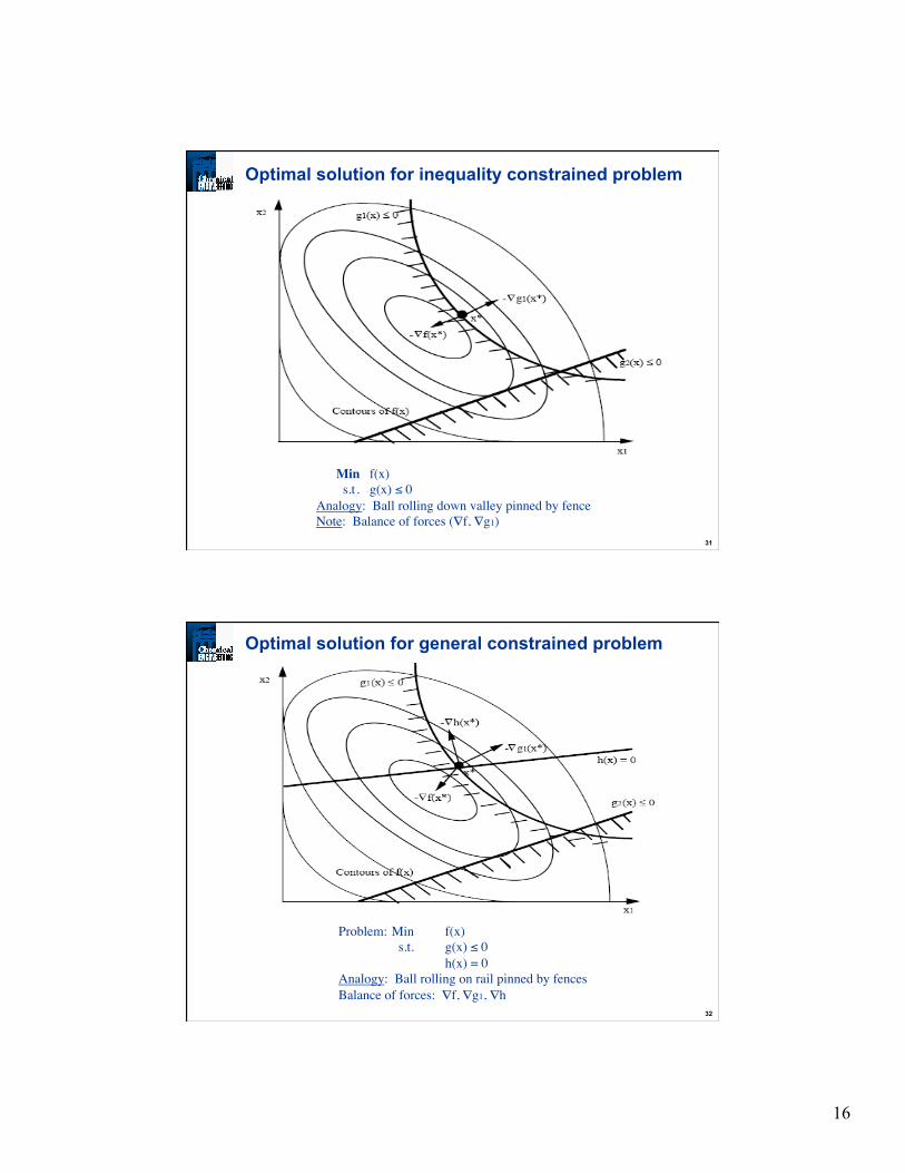
Optimal solution for inequality constrained problem
Min f(x)
s.t . g(x) ≤ 0
Analogy: Ball rolling down valley pinned by fence
Note: Balance of forces (∇f, ∇g1)
32
Optimal solution for general constrained problem
Problem: Min f(x)
s.t. g(x) ≤ 0
h(x) = 0
Analogy: Ball rolling on rail pinned by fences
Balance of forces: ∇f, ∇g1, ∇h
17
33
Necessary First Order Karush Kuhn - Tucker Conditions
∇ L (x*, u, v) = ∇f(x*) + ∇g(x*) u + ∇h(x*) v = 0 (Balance of Forces) u ≥ 0 (Inequalities act in only one direction) g (x*) ≤ 0, h (x*) = 0 (Feasibility) uj gj(x*) = 0 (Complementarity: either gj(x*) = 0 or uj = 0)
u, v are "weights" for "forces," known as KKT multipliers, shadow prices, dual variables
“To guarantee that a local NLP solution satisfies KKT conditions, a constraint qualification is required. E.g., the Linear Independence Constraint Qualification (LICQ) requires active constraint gradients, [∇gA(x*) ∇h(x*)], to be linearly independent. Also, under LICQ, KKT multipliers are uniquely determined.” Necessary (Sufficient) Second Order Conditions - Positive curvature in "constraint" directions. - pT∇ 2L (x*) p ≥ 0 (pT∇ 2L (x*) p > 0) where p are the constrained directions: ∇h(x*)Tp = 0
for gi(x*)=0, ∇gi(x*)Tp = 0, for ui > 0, ∇gi(x*)Tp ≤ 0, for ui = 0
Optimality conditions for local optimum
34
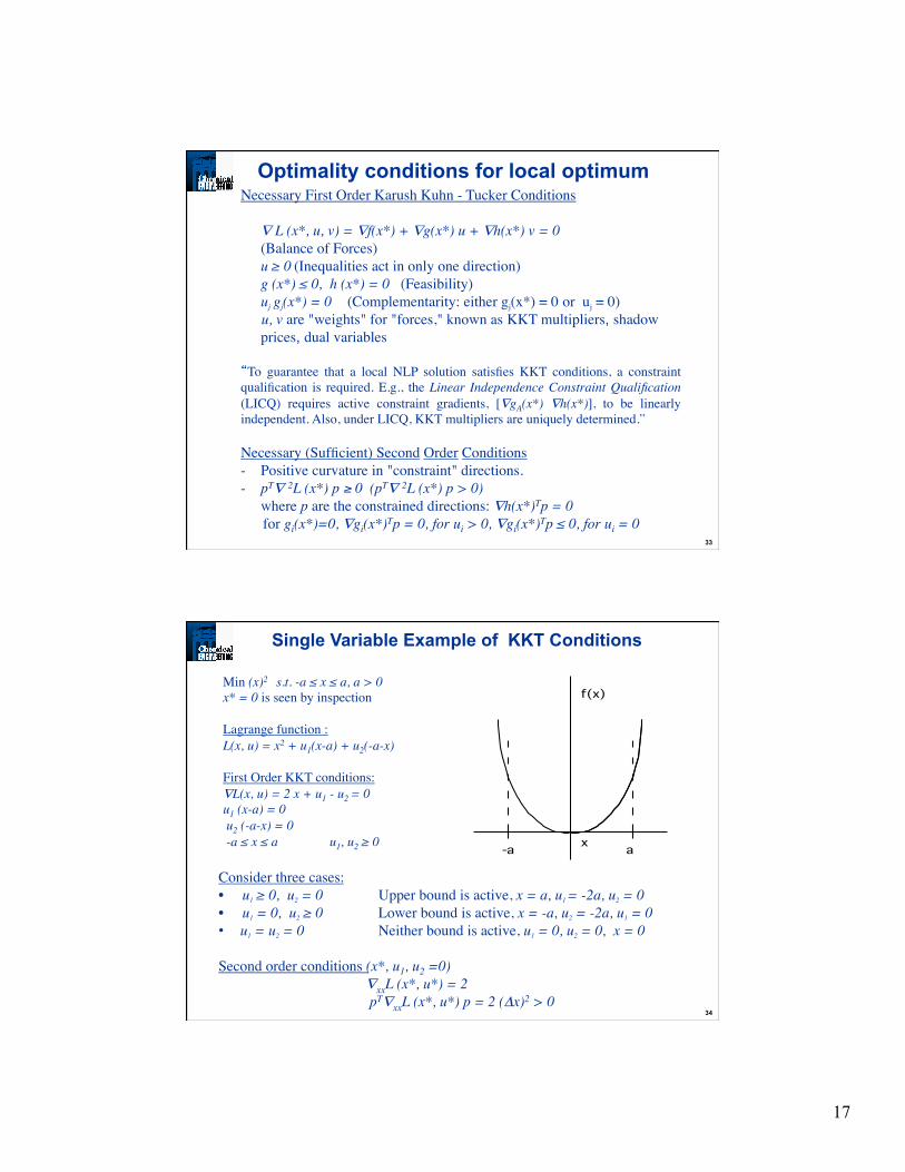
Single Variable Example of KKT Conditions
-a a
f(x)
x
Min (x)2 s.t. -a ≤ x ≤ a, a > 0
x* = 0 is seen by inspection Lagrange function : L(x, u) = x2 + u1(x-a) + u2(-a-x)
First Order KKT conditions:
∇L(x, u) = 2 x + u1 - u2 = 0
u1 (x-a) = 0 u2 (-a-x) = 0
-a ≤ x ≤ a u1, u2 ≥ 0
Consider three cases: • u1 ≥ 0, u2 = 0 Upper bound is active, x = a, u1 = -2a, u2 = 0 • u1 = 0, u2 ≥ 0 Lower bound is active, x = -a, u2 = -2a, u1 = 0 • u1 = u2 = 0 Neither bound is active, u1 = 0, u2 = 0, x = 0 Second order conditions (x*, u1, u2 =0)
∇xxL (x*, u*) = 2 pT∇xxL (x*, u*) p = 2 (Δx)2 > 0
18
35
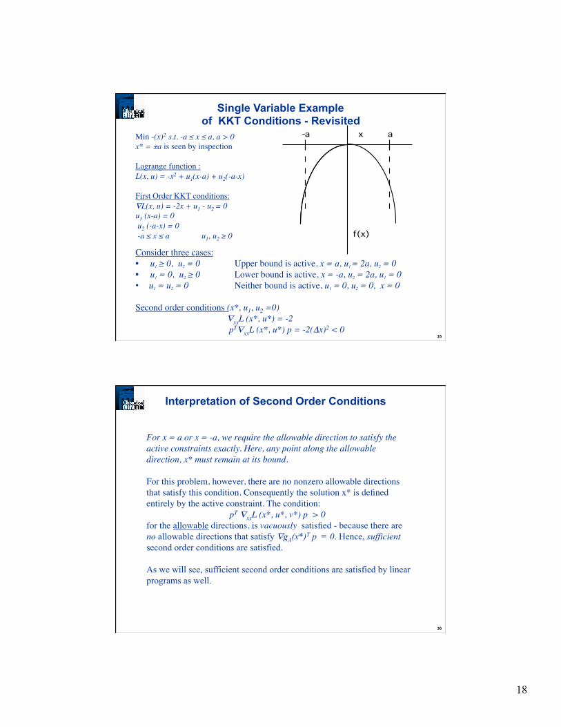
Single Variable Example of KKT Conditions - Revisited
Min -(x)2 s.t. -a ≤ x ≤ a, a > 0
x* = ±a is seen by inspection Lagrange function : L(x, u) = -x2 + u1(x-a) + u2(-a-x)
First Order KKT conditions:
∇L(x, u) = -2x + u1 - u2 = 0
u1 (x-a) = 0 u2 (-a-x) = 0
-a ≤ x ≤ a u1, u2 ≥ 0
Consider three cases: • u1 ≥ 0, u2 = 0 Upper bound is active, x = a, u1 = 2a, u2 = 0 • u1 = 0, u2 ≥ 0 Lower bound is active, x = -a, u2 = 2a, u1 = 0 • u1 = u2 = 0 Neither bound is active, u1 = 0, u2 = 0, x = 0 Second order conditions (x*, u1, u2 =0)
∇xxL (x*, u*) = -2 pT∇xxL (x*, u*) p = -2(Δx)2 < 0
a-a
f(x)
x
36
For x = a or x = -a, we require the allowable direction to satisfy the active constraints exactly. Here, any point along the allowable direction, x* must remain at its bound. For this problem, however, there are no nonzero allowable directions that satisfy this condition. Consequently the solution x* is defined entirely by the active constraint. The condition:
pT ∇xxL (x*, u*, v*) p > 0 for the allowable directions, is vacuously satisfied - because there are no allowable directions that satisfy ∇gA(x*)T p = 0. Hence, sufficient second order conditions are satisfied. As we will see, sufficient second order conditions are satisfied by linear programs as well.
Interpretation of Second Order Conditions
19
37
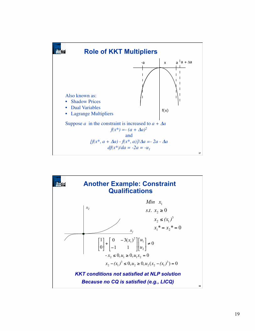
Role of KKT Multipliers a-a
f(x)
x a + Δa
Also known as: • Shadow Prices
• Dual Variables
• Lagrange Multipliers
Suppose a in the constraint is increased to a + Δa
f(x*) =- (a + Δa)2
and [f(x*, a + Δa) - f(x*, a)]/Δa =- 2a - Δa
df(x*)/da = -2a = -u1
38
Another Example: Constraint Qualifications
0**
0 ..
21
312
2
1
==
≤
≥
xx)(xx
xtsxMin
0)(,0,0
0,0,0-
011
)(3001
31222
312
2112
2
12
1
=−≥≤−
=≥≤
≠
−
−+
)(xxuu)(xxxuuxuux
x1
x2
KKT conditions not satisfied at NLP solution Because no CQ is satisfied (e.g., LICQ)
20
39
Motivation: Build on unconstrained methods wherever possible. Classification of Methods:
• Reduced Gradient Methods - (with Restoration) GRG2, CONOPT • Reduced Gradient Methods - (without Restoration) MINOS • Successive Quadratic Programming - generic implementations • Penalty Functions - popular in 1970s, but fell into disfavor. Barrier Methods have been developed recently and are again popular. • Successive Linear Programming - only useful for "mostly linear" problems
We will concentrate on algorithms for first four classes. Evaluation: Compare performance on "typical problem," cite experience on process problems.
Algorithms for Constrained Problems
40
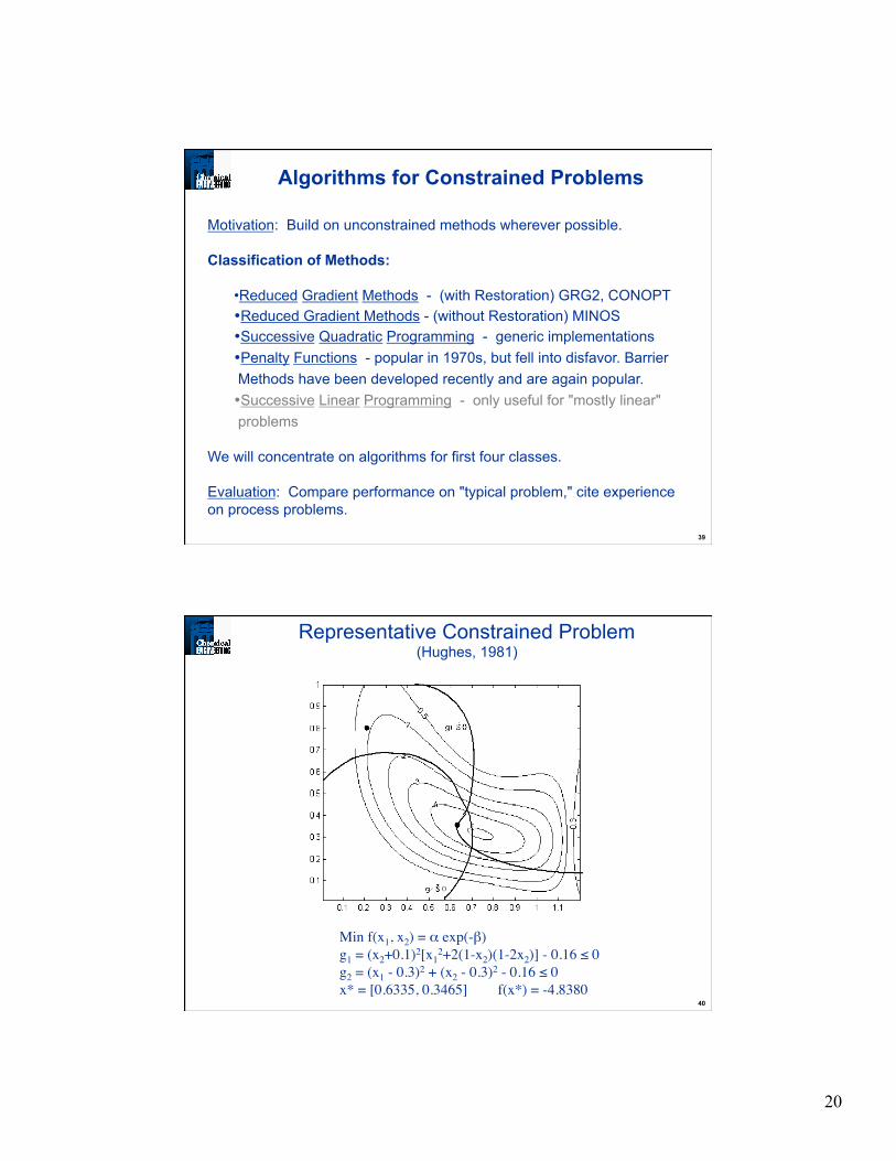
Representative Constrained Problem
(Hughes, 1981)
Min f(x1, x2) = α exp(-β) g1 = (x2+0.1)2[x1
2+2(1-x2)(1-2x2)] - 0.16 ≤ 0 g2 = (x1 - 0.3)2 + (x2 - 0.3)2 - 0.16 ≤ 0 x* = [0.6335, 0.3465] f(x*) = -4.8380

21
41
Min f(x) Min f(z) s.t. g(x) + s = 0 (add slack variable) `⇒ s.t. c(z) = 0 h(x) = 0 a ≤ z ≤ b a ≤ x ≤ b, s ≥ 0
Partition variables into: zB - dependent or basic variables zN - nonbasic variables, fixed at a bound zS - independent or superbasic variables
Reduced Gradient Method with Restoration (GRG2/CONOPT)
!
Modified KKT Conditions
"f (z) +"c(z)# $% L + %U = 0
c(z) = 0
z(i)
= zU(i)
or z(i)
= zL(i)
, i & N
%U( i)
, % L
( i) = 0, i ' N
42
• Solve bound constrained problem in space of superbasic variables (apply gradient projection algorithm)
• Solve (e) to eliminate zB
• Use (a) and (b) to calculate reduced gradient wrt zS.
• Nonbasic variables zN (temporarily) fixed (d) • Repartition based on signs of ν, if zs remain at bounds or if zB violate bounds
Reduced Gradient Method with Restoration (GRG2/CONOPT)
!
a) "S f (z) +"Sc(z)# = 0
b) "B f (z) +"Bc(z)# = 0
c) "N f (z) +"Nc(z)# $% L + %U = 0
d) z( i)
= zU( i)
or z( i)
= zL( i)
, i & N
e) c(z) = 0' zB = zB (zS )
22
43
• By remaining feasible always, c(z) = 0, a ≤ z ≤ b, one can apply an unconstrained algorithm (quasi-Newton) using (df/dzS), using (b) • Solve problem in reduced space of zS variables, using (e).
Definition of Reduced Gradient
!
df
dzS="f
"zS+dzB
dzS
"f
"zBBecause c(z) = 0,we have :
dc ="c
"zS
#
$ %
&
' (
T
dzS +"c
"zB
#
$ %
&
' (
T
dzB = 0
dzB
dzS= )
"c
"zS
#
$ %
&
' ( "c
"zB
#
$ %
&
' (
)1
= )* zSc * zB
c[ ])1
This leads to :
df
dzS=*S f (z) )*Sc *Bc[ ]
)1*B f (z) =*S f (z) +*Sc(z)+
44
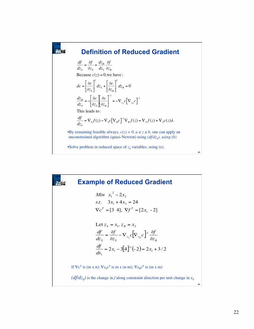
If ∇cT is (m x n); ∇zScT is m x (n-m); ∇zBcT is (m x m) (df/dzS) is the change in f along constraint direction per unit change in zS
Example of Reduced Gradient
[ ]
[ ] ( ) 2/322-432
Let
2]- 2[ 4], 3[
2443 ..2
11
11
1
21
1
21
22
1
+=−=
∂
∂∇∇−
∂
∂=
==
=∇=∇
=+
−
−
−
xxdxdf
zfcc
zf
dzdf
x, zxz
xfcxxtsxxMin
Bzz
SS
BS
TT
BS
23
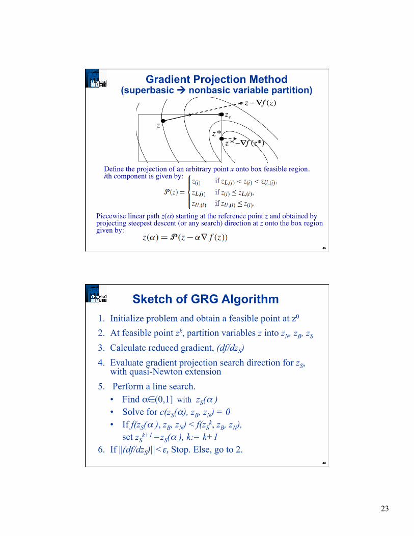
45
Gradient Projection Method (superbasic nonbasic variable partition)
Define the projection of an arbitrary point x onto box feasible region. ith component is given by:
Piecewise linear path z(α) starting at the reference point z and obtained by projecting steepest descent (or any search) direction at z onto the box region given by:
46
Sketch of GRG Algorithm 1. Initialize problem and obtain a feasible point at z0
2. At feasible point zk, partition variables z into zN, zB, zS 3. Calculate reduced gradient, (df/dzS) 4. Evaluate gradient projection search direction for zS,
with quasi-Newton extension 5. Perform a line search.
• Find α∈(0,1] with zS(α ) • Solve for c(zS(α), zB, zN) = 0 • If f(zS(α ), zB, zN) < f(zS
k, zB, zN), set zS
k+1 =zS(α ), k:= k+1 6. If ||(df/dzS)||<ε, Stop. Else, go to 2.

24
47
Reduced Gradient Method with Restoration
zS
zB
48
Reduced Gradient Method with Restoration
zS
zB
Fails, due to singularity in basis matrix (dc/dzB)
25
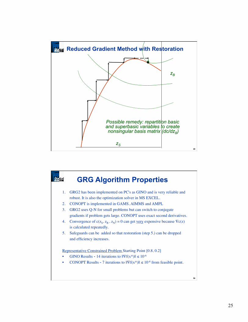
49
Reduced Gradient Method with Restoration
zS
zB
Possible remedy: repartition basic and superbasic variables to create nonsingular basis matrix (dc/dzB)
50
1. GRG2 has been implemented on PC's as GINO and is very reliable and robust. It is also the optimization solver in MS EXCEL.
2. CONOPT is implemented in GAMS, AIMMS and AMPL 3. GRG2 uses Q-N for small problems but can switch to conjugate
gradients if problem gets large. CONOPT uses exact second derivatives. 4. Convergence of c(zS, zB , zN) = 0 can get very expensive because ∇c(z)
is calculated repeatedly. 5. Safeguards can be added so that restoration (step 5.) can be dropped
and efficiency increases. Representative Constrained Problem Starting Point [0.8, 0.2] • GINO Results - 14 iterations to ||∇f(x*)|| ≤ 10-6 • CONOPT Results - 7 iterations to ||∇f(x*)|| ≤ 10-6 from feasible point.
GRG Algorithm Properties
26
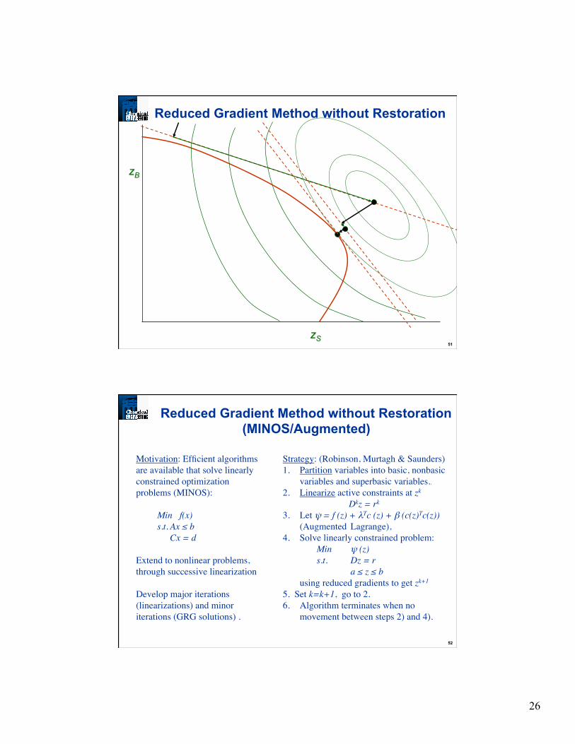
51
Reduced Gradient Method without Restoration
zS
zB
52
Motivation: Efficient algorithms are available that solve linearly constrained optimization problems (MINOS): Min f(x) s.t. Ax ≤ b Cx = d
Extend to nonlinear problems, through successive linearization Develop major iterations (linearizations) and minor iterations (GRG solutions) .
Reduced Gradient Method without Restoration (MINOS/Augmented)
Strategy: (Robinson, Murtagh & Saunders) 1. Partition variables into basic, nonbasic
variables and superbasic variables.. 2. Linearize active constraints at zk
Dkz = rk 3. Let ψ = f (z) + λTc (z) + β (c(z)Tc(z))
(Augmented Lagrange), 4. Solve linearly constrained problem:
Min ψ (z) s.t. Dz = r a ≤ z ≤ b
using reduced gradients to get zk+1 5. Set k=k+1, go to 2. 6. Algorithm terminates when no
movement between steps 2) and 4).
27
53
1. MINOS has been implemented very efficiently to take care of linearity. It becomes LP Simplex method if problem is totally linear. Also, very efficient matrix routines.
2. No restoration takes place, nonlinear constraints are reflected in ψ(z) during step 3). MINOS is more efficient than GRG.
3. Major iterations (steps 3) - 4)) converge at a quadratic rate. 4. Reduced gradient methods are complicated, monolithic codes:
hard to integrate efficiently into modeling software. Representative Constrained Problem – Starting Point [0.8, 0.2] MINOS Results: 4 major iterations, 11 function calls to ||∇f(x*)|| ≤ 10-6 �
MINOS/Augmented Notes
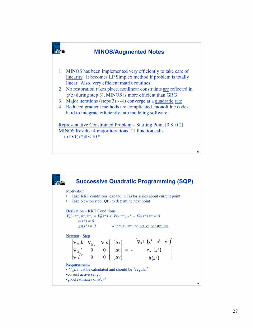
54
Motivation: • Take KKT conditions, expand in Taylor series about current point. • Take Newton step (QP) to determine next point. Derivation – KKT Conditions ∇xL (x*, u*, v*) = ∇f(x*) + ∇gA(x*) u* + ∇h(x*) v* = 0
h(x*) = 0 gA(x*) = 0, where gA are the active constraints.
Newton - Step
xx∇ LAg∇ ∇ h
Ag∇ T 0 0
∇ hT 0 0
ΔxΔuΔv
= -
x∇ L kx , ku , kv( )
Ag kx( )h kx( )
Requirements: • ∇xxL must be calculated and should be ‘regular’ • correct active set gA • good estimates of uk, vk
Successive Quadratic Programming (SQP)

28
55
1. Wilson (1963) - active set can be determined by solving QP: Min ∇f(xk)Td + 1/2 dT ∇xx L(xk, uk, vk) d d s.t. g(xk) + ∇g(xk)T d ≤ 0 h(xk) + ∇h(xk)T d = 0
2. Han (1976), (1977), Powell (1977), (1978) - approximate ∇xxL using a positive definite quasi-Newton update (BFGS) - use a line search to converge from poor starting points. Notes: - Similar methods were derived using penalty (not Lagrange) functions. - Method converges quickly; very few function evaluations. - Not well suited to large problems (full space update used). For n > 100, say, use reduced space methods (e.g. MINOS).
SQP Chronology
56
What about ∇xxL?
• need to get second derivatives for f(x), g(x), h(x). • need to estimate multipliers, uk, vk; ∇xxL may not be positive semidefinite ⇒ Approximate ∇xxL (xk, uk, vk) by Bk, a symmetric positive definite matrix. BFGS Formula s = xk+1 - xk
y = ∇L(xk+1, uk+1, vk+1) - ∇L(xk, uk+1, vk+1) • second derivatives approximated by change in gradients • positive definite Bk ensures unique QP solution
Elements of SQP – Hessian Approximation
!
k+1
B = k
B +
TyyTs y
-
kB s T
sk
Bk
s B s

29
57
How do we obtain search directions? • Form QP and let QP determine constraint activity • At each iteration, k, solve:
Min ∇f(xk) Td + 1/2 dT Bkd d s.t. g(xk) + ∇g(xk) T d ≤ 0 h(xk) + ∇h(xk) T d = 0
Convergence from poor starting points • As with Newton's method, choose α (stepsize) to ensure progress toward optimum: xk+1 = xk + α d. • α is chosen by making sure a merit function is decreased at each iteration.
Exact Penalty Function ψ(x) = f(x) + µ [Σ max (0, gj(x)) + Σ |hj (x)|] µ > maxj {| uj |, | vj |} Augmented Lagrange Function ψ(x) = f(x) + uTg(x) + vTh(x) + η/2 {Σ (hj (x))2 + Σ max (0, gj (x))2}
Elements of SQP – Search Directions
58
Fast Local Convergence B = ∇xxL Quadratic ∇xxL is p.d and B is Q-N 1 step Superlinear B is Q-N update, ∇xxL not p.d 2 step Superlinear Enforce Global Convergence Ensure decrease of merit function by taking α ≤ 1 Trust region adaptations provide a stronger guarantee of global convergence - but harder to implement.
Newton-Like Properties for SQP
30
59
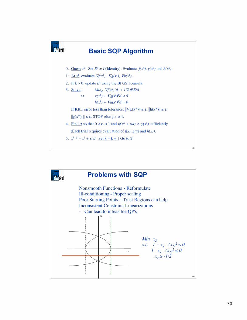
0. Guess x0, Set B0 = I (Identity). Evaluate f(x0), g(x0) and h(x0).
1. At xk, evaluate ∇f(xk), ∇g(xk), ∇h(xk).
2. If k > 0, update Bk using the BFGS Formula. 3. Solve: Mind ∇f(xk)Td + 1/2 dTBkd s.t. g(xk) + ∇g(xk)Td ≤ 0 h(xk) + ∇h(xk)Td = 0
If KKT error less than tolerance: ||∇L(x*)|| ≤ ε, ||h(x*)|| ≤ ε,
||g(x*)+|| ≤ ε. STOP, else go to 4.
4. Find α so that 0 < α ≤ 1 and ψ(xk + αd) < ψ(xk) sufficiently
(Each trial requires evaluation of f(x), g(x) and h(x)).
5. xk+1 = xk + α d. Set k = k + 1 Go to 2.
Basic SQP Algorithm
60
Nonsmooth Functions - Reformulate
Ill-conditioning - Proper scaling
Poor Starting Points – Trust Regions can help
Inconsistent Constraint Linearizations
- Can lead to infeasible QP's
x2
x1
Min x2 s.t. 1 + x1 - (x2)2 ≤ 0 1 - x1 - (x2)2 ≤ 0 x2 ≥ -1/2
Problems with SQP

31
61
SQP Test Problem
1.21.00.80.60.40.20.00.0
0.2
0.4
0.6
0.8
1.0
1.2
x1
x2
x*
Min x2 s.t. -x2 + 2 x1
2 - x13 ≤ 0
-x2 + 2 (1-x1)2 - (1-x1)3 ≤ 0 x* = [0.5, 0.375].
62
SQP Test Problem – First Iteration
1.21.00.80.60.40.20.00.0
0.2
0.4
0.6
0.8
1.0
1.2
x1
x2
Start from the origin (x0 = [0, 0]T) with B0 = I, form: Min d2 + 1/2 (d1
2 + d22)
s.t. d2 ≥ 0 d1 + d2 ≥ 1 d = [1, 0]T. with µ1 = 0 and µ2 = 1.

32
63
1.21.00.80.60.40.20.00.0
0.2
0.4
0.6
0.8
1.0
1.2
x1
x2
x*
From x1 = [0.5, 0]T with B1 = I (no update from BFGS possible), form: Min d2 + 1/2 (d1
2 + d22)
s.t. -1.25 d1 - d2 + 0.375 ≤ 0 1.25 d1 - d2 + 0.375 ≤ 0 d = [0, 0.375]T with µ1 = 0.5 and µ2 = 0.5 x* = [0.5, 0.375]T is optimal
SQP Test Problem – Second Iteration
64
Representative Constrained Problem
SQP Convergence Path
Starting Point [0.8, 0.2] - starting from B0 = I and staying in bounds and linearized constraints; converges in 8 iterations to ||∇f(x*)|| ≤ 10-6
33
65
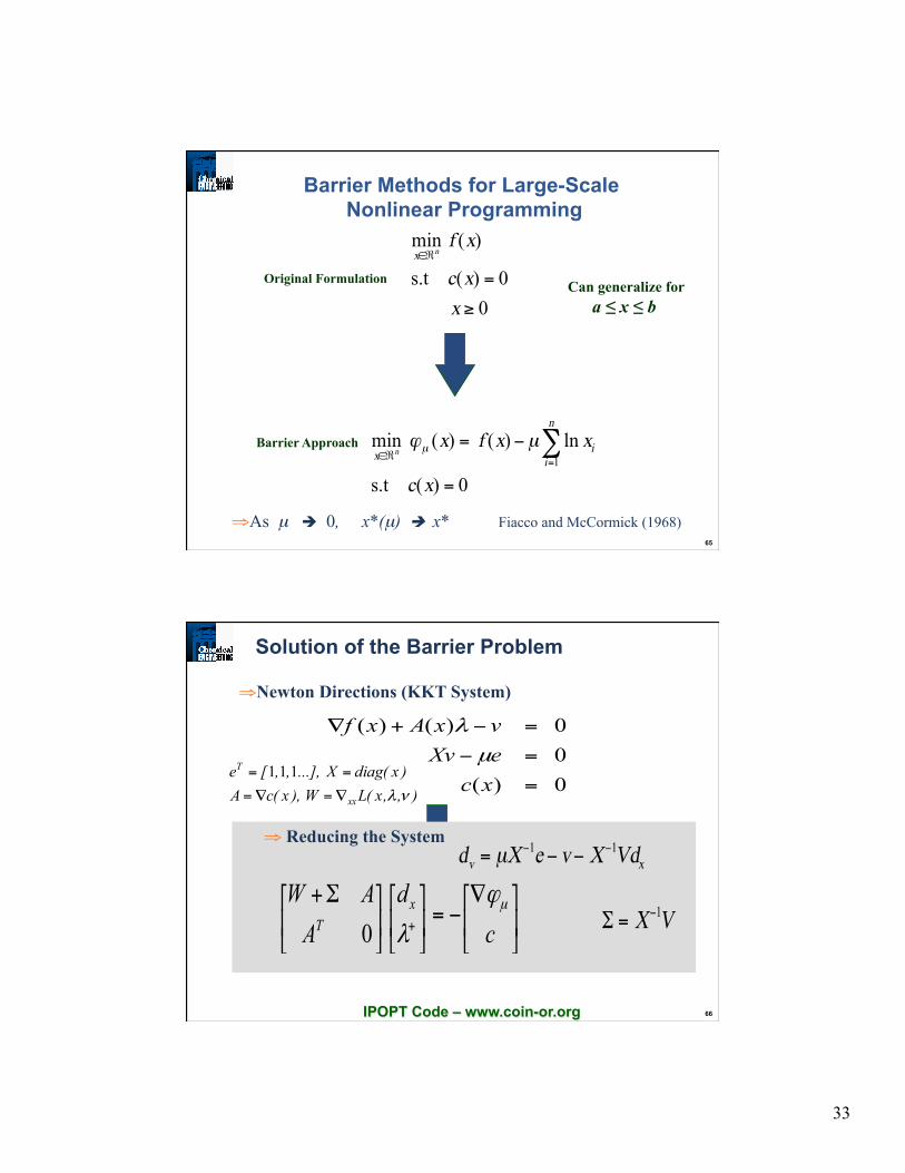
Barrier Methods for Large-Scale Nonlinear Programming
0
0)(s.t
)(min
!
=
"#
x
xc
xfnx
Original Formulation
0)(s.t
ln)()( min1
=
!= "=
#$
xc
xxfxn
i
ix n
µ%µBarrier Approach
Can generalize for a ≤ x ≤ b
⇒ As µ 0, x*(µ) x* Fiacco and McCormick (1968)
66
Solution of the Barrier Problem
⇒ Newton Directions (KKT System)
0 )(0 0 )()(
=
=−
=−+∇
xceXvvxAxfµ
λ
⇒ Solve
−
−+∇
−=
−
eXvc
vAf
ddd
XVA
IAW xT
000
µ
λ
ν
λ
⇒ Reducing the System xv
VdXveXd11 !!
!!= µ
∇−=
Σ++ cd
AAW x
Tµϕ
λ
0 VX1!
="
IPOPT Code – www.coin-or.org
),,x(LW),x(cA)x(diagX...],,,[e
xx
T
νλ∇=∇=
==
1 1 1
34
67
Global Convergence of Newton-based Barrier Solvers
Merit Function
Exact Penalty: P(x, η) = f(x) + η ||c(x)||
Aug’d Lagrangian: L*(x, λ, η) = f(x) + λTc(x) + η ||c(x)||2
Assess Search Direction (e.g., from IPOPT)
Line Search – choose stepsize α to give sufficient decrease of merit function using a ‘step to the boundary’ rule with τ ~0.99.
• How do we balance φ (x) and c(x) with η? • Is this approach globally convergent? Will it still be fast?
)( 0)1(
0)1( ],,0( for
1
1
1
kkk
kvkk
kxk
xkk
vdvvxdx
dxx
λλαλλ
τα
τα
ααα
−+=
>−≥+=
>−≥+
+=∈
++
+
+
68
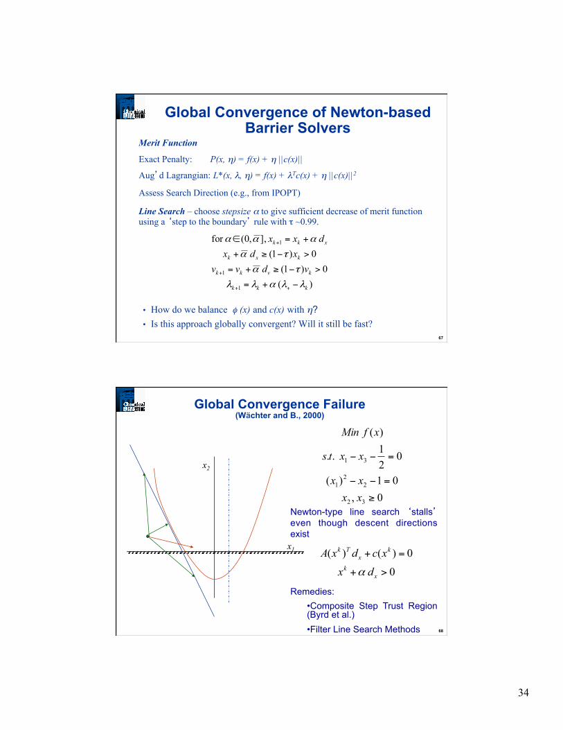
Global Convergence Failure (Wächter and B., 2000)
0 ,01)(
021 ..
)(
32
22
1
31
≥
=−−
=−−
xxxx
xxts
xfMin
x1
x2
0
0)()(
>+
=+
xk
kx
Tk
dxxcdxA
α
Newton-type line search ‘stalls’ even though descent directions exist Remedies:
• Composite Step Trust Region (Byrd et al.) • Filter Line Search Methods

35
69
Line Search Filter Method
Store (φk, θk) at allowed iterates
Allow progress if trial point is acceptable to filter with θ margin
If switching condition
is satisfied, only an Armijo line search is required on φk
If insufficient progress on stepsize, evoke restoration phase to reduce θ.
Global convergence and superlinear local convergence proved (with second order correction)
22,][][ >>≥−∇ bad bk
aTk θδφα
φ(x)
θ(x) = ||c(x)||
70
Implementation Details
Modify KKT (full space) matrix if singular
• δ1 - Correct inertia to guarantee descent direction • δ2 - Deal with rank deficient Ak
KKT matrix factored by MA27
Feasibility restoration phase
Apply Exact Penalty Formulation
Exploit same structure/algorithm to reduce infeasibility
!"
#$%
&
'
+(+
IA
AW
T
k
kkk
2
1
)
)
ukl
Qk
xxx
xxxcMin
!!
"+2
1 ||||||)(||
36
71
IPOPT Algorithm – Features
Line Search Strategies for Globalization
- l2 exact penalty merit function
- augmented Lagrangian merit function
- Filter method (adapted and extended from Fletcher and Leyffer)
Hessian Calculation
- BFGS (full/LM and reduced space)
- SR1 (full/LM and reduced space)
- Exact full Hessian (direct)
- Exact reduced Hessian (direct)
- Preconditioned CG
Algorithmic Properties Globally, superlinearly convergent (Wächter and B., 2005) Easily tailored to different problem structures
Freely Available
CPL License and COIN-OR distribution: http://www.coin-or.org IPOPT 3.1 recently rewritten in C++ Solved on thousands of test problems and applications
72
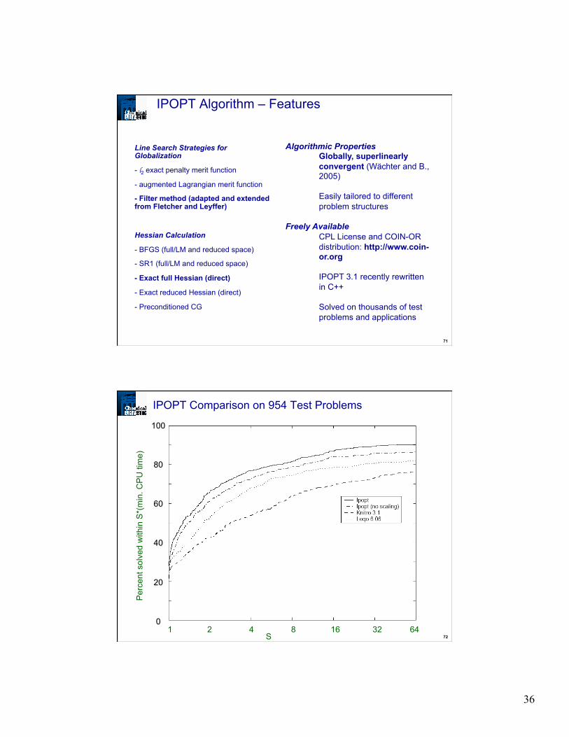
IPOPT Comparison on 954 Test Problems
1248163264 S
Per
cent
sol
ved
with
in S
*(m
in. C
PU
tim
e)
100 80 60 40 20 0
37
73
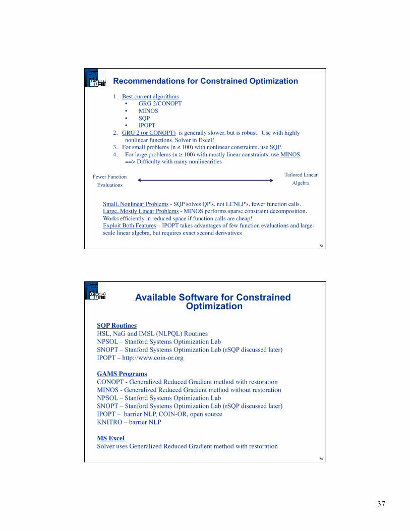
Recommendations for Constrained Optimization
1. Best current algorithms
• GRG 2/CONOPT
• MINOS
• SQP • IPOPT
2. GRG 2 (or CONOPT) is generally slower, but is robust. Use with highly nonlinear functions. Solver in Excel!
3. For small problems (n ≤ 100) with nonlinear constraints, use SQP. 4. For large problems (n ≥ 100) with mostly linear constraints, use MINOS.
==> Difficulty with many nonlinearities
Small, Nonlinear Problems - SQP solves QP's, not LCNLP's, fewer function calls. Large, Mostly Linear Problems - MINOS performs sparse constraint decomposition. Works efficiently in reduced space if function calls are cheap! Exploit Both Features – IPOPT takes advantages of few function evaluations and large-scale linear algebra, but requires exact second derivatives
Fewer Function Evaluations
Tailored Linear Algebra
74
SQP Routines HSL, NaG and IMSL (NLPQL) Routines NPSOL – Stanford Systems Optimization Lab SNOPT – Stanford Systems Optimization Lab (rSQP discussed later) IPOPT – http://www.coin-or.org GAMS Programs CONOPT - Generalized Reduced Gradient method with restoration MINOS - Generalized Reduced Gradient method without restoration NPSOL – Stanford Systems Optimization Lab SNOPT – Stanford Systems Optimization Lab (rSQP discussed later) IPOPT – barrier NLP, COIN-OR, open source KNITRO – barrier NLP MS Excel Solver uses Generalized Reduced Gradient method with restoration
Available Software for Constrained Optimization
38
75
1) Avoid overflows and undefined terms, (do not divide, take logs, etc.) e.g. x + y - ln z = 0 x + y - u = 0 exp u - z = 0
2) If constraints must always be enforced, make sure they are linear or bounds. e.g. v(xy - z2)1/2 = 3 vu = 3 u2 - (xy - z2) = 0, u ≥ 0
3) Exploit linear constraints as much as possible, e.g. mass balance xi L + yi V = F zi li + vi = fi
L – ∑ li = 0 4) Use bounds and constraints to enforce characteristic solutions. e.g. a ≤ x ≤ b, g (x) ≤ 0 to isolate correct root of h (x) = 0.
5) Exploit global properties when possibility exists. Convex (linear equations?) Linear Program? Quadratic Program? Geometric Program? 6) Exploit problem structure when possible. e.g. Min [Tx - 3Ty] s.t. xT + y - T2 y = 5 4x - 5Ty + Tx = 7 0 ≤ T ≤ 1
(If T is fixed ⇒ solve LP) ⇒ put T in outer optimization loop.
Rules for Formulating Nonlinear Programs
76
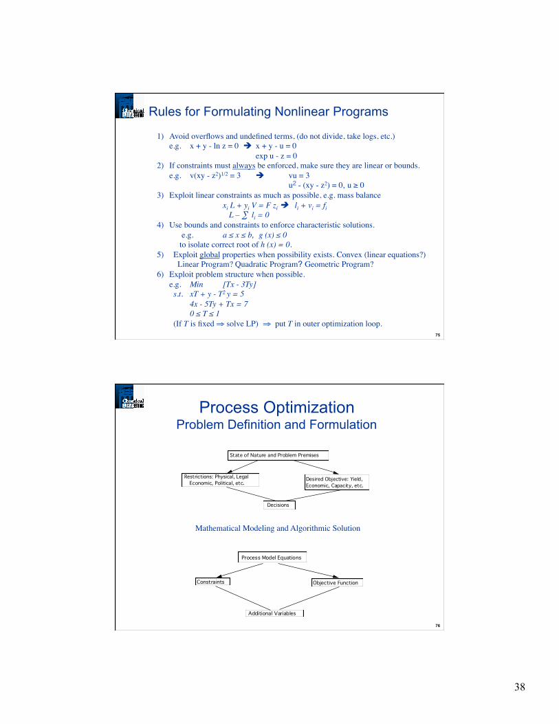
State of Nature and Problem Premises
Restrictions: Physical, LegalEconomic, Political, etc.
Desired Objective: Yield, Economic, Capacity, etc.
Decisions
Process Model Equations
Constraints Objective Function
Additional Variables
Process Optimization
Problem Definition and Formulation
Mathematical Modeling and Algorithmic Solution
39
77
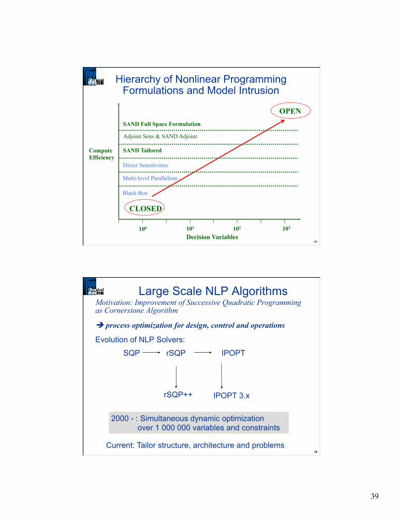
Hierarchy of Nonlinear Programming Formulations and Model Intrusion
CLOSED
OPEN
Decision Variables 101 102 103
Black Box
Direct Sensitivities
Multi-level Parallelism
SAND Tailored
Adjoint Sens & SAND Adjoint
SAND Full Space Formulation
100
Compute Efficiency
78
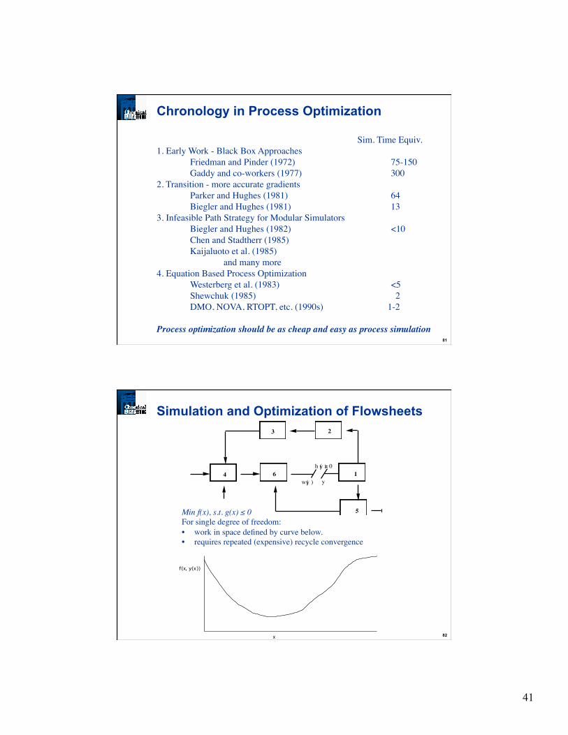
Large Scale NLP Algorithms Motivation: Improvement of Successive Quadratic Programming as Cornerstone Algorithm
process optimization for design, control and operations
Evolution of NLP Solvers:
1981-87: Flowsheet optimization over 100 variables and constraints
1988-98: Static Real-time optimization over 100 000 variables and constraints 2000 - : Simultaneous dynamic optimization over 1 000 000 variables and constraints
SQP rSQP IPOPT
rSQP++
Current: Tailor structure, architecture and problems
IPOPT 3.x

40
79
In Out
Modular Simulation Mode
Physical Relation to Process
- Intuitive to Process Engineer
- Unit equations solved internally - tailor-made procedures.
• Convergence Procedures - for simple flowsheets, often identified from flowsheet structure
• Convergence "mimics" startup. • Debugging flowsheets on "physical" grounds
Flowsheet Optimization Problems - Introduction
80
C
13
2 4
Design Specifications
Specify # trays reflux ratio, but would like to specify overhead comp. ==> Control loop -Solve Iteratively
• Frequent block evaluation can be expensive • Slow algorithms applied to flowsheet loops. • NLP methods are good at breaking loops
Flowsheet Optimization Problems - Features
Nested Recycles Hard to Handle
Best Convergence Procedure?
41
81
Chronology in Process Optimization
Sim. Time Equiv. 1. Early Work - Black Box Approaches
Friedman and Pinder (1972) 75-150 Gaddy and co-workers (1977) 300
2. Transition - more accurate gradients Parker and Hughes (1981) 64 Biegler and Hughes (1981) 13
3. Infeasible Path Strategy for Modular Simulators Biegler and Hughes (1982) <10 Chen and Stadtherr (1985) Kaijaluoto et al. (1985) and many more
4. Equation Based Process Optimization Westerberg et al. (1983) <5 Shewchuk (1985) 2 DMO, NOVA, RTOPT, etc. (1990s) 1-2
Process optimization should be as cheap and easy as process simulation
82
4
3 2
1
5
6h (y ) = 0
w(y ) y
f(x, y(x))
x
Simulation and Optimization of Flowsheets
Min f(x), s.t. g(x) ≤ 0
For single degree of freedom:
• work in space defined by curve below. • requires repeated (expensive) recycle convergence
�
42
83
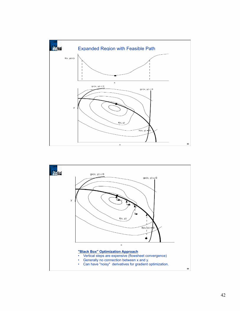
Expanded Region with Feasible Path
�
84
"Black Box" Optimization Approach
• Vertical steps are expensive (flowsheet convergence)
• Generally no connection between x and y. • Can have "noisy" derivatives for gradient optimization.
43
85
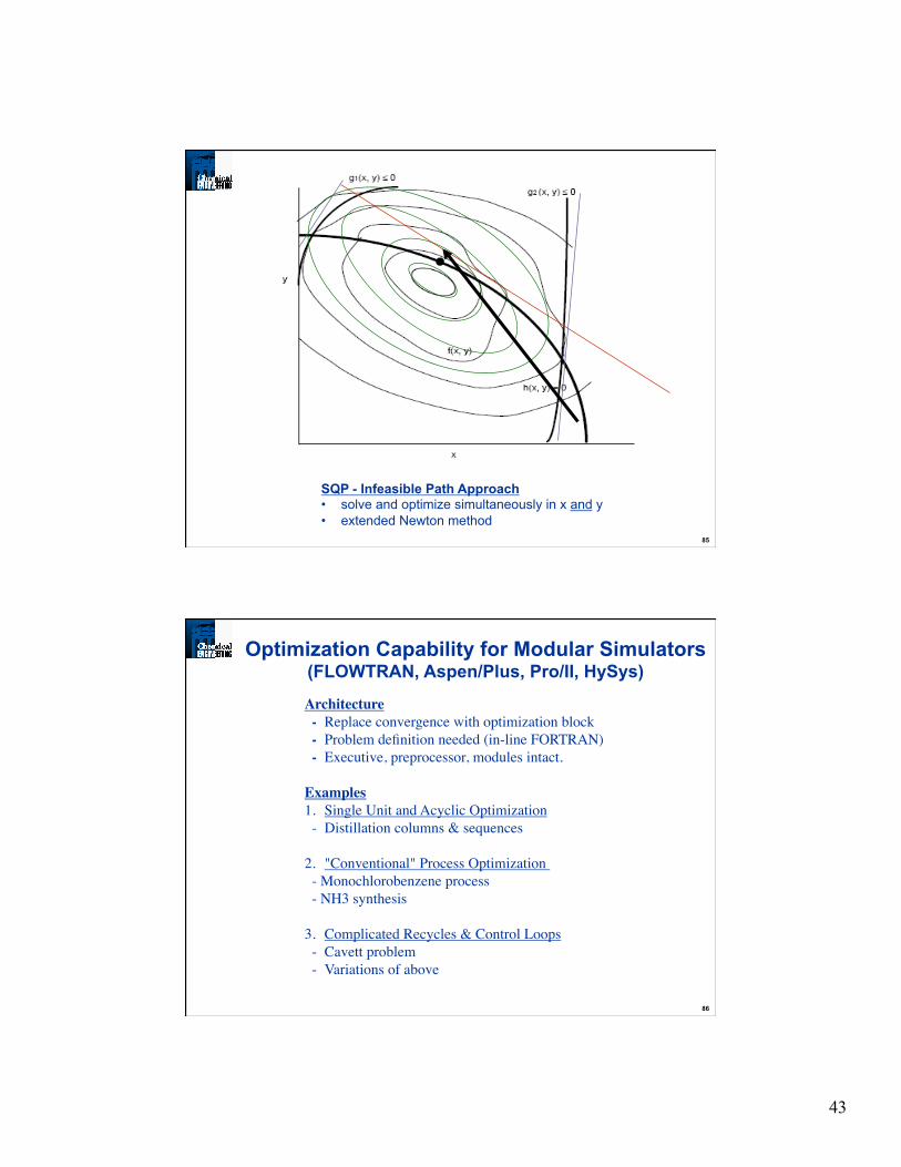
SQP - Infeasible Path Approach
• solve and optimize simultaneously in x and y • extended Newton method
86
Architecture - Replace convergence with optimization block - Problem definition needed (in-line FORTRAN) - Executive, preprocessor, modules intact. Examples 1. Single Unit and Acyclic Optimization - Distillation columns & sequences 2. "Conventional" Process Optimization - Monochlorobenzene process - NH3 synthesis 3. Complicated Recycles & Control Loops - Cavett problem - Variations of above
Optimization Capability for Modular Simulators (FLOWTRAN, Aspen/Plus, Pro/II, HySys)
44
87
S06HC1
A-1ABSORBER
15 Trays(3 Theoret ical Stages)
32 psia
P
S04Fe ed80
oF
37 psia
T
270o F
S01 S02
Steam360o F
H-1U = 100
MaximizeProfit
Fe ed F low RatesLB Moles/Hr
HC1 10Benzene 40MCB 50
S07
S08
S05
S09
HC1
T-1TREATER
F-1FLASH
S03
S10
25ps ia
S12
S13S15
P-1C
1200 FT
MCB
S14
U = 100 CoolingWater80o F
S11
Benzene,0.1 Lb Mole/Hr
of MC B
D-1DISTILLATION
30 Trays(20 Theoreti cal Stages)
Steam360oF
12,000Btu/hr- ft2
90oFH-2
U = 100
Water80oF
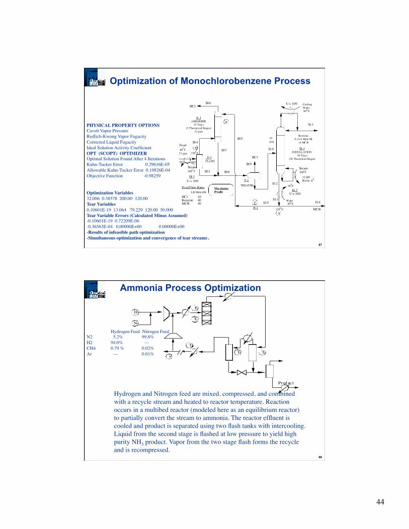
PHYSICAL PROPERTY OPTIONS Cavett Vapor Pressure Redlich-Kwong Vapor Fugacity Corrected Liquid Fugacity Ideal Solution Activity Coefficient OPT (SCOPT) OPTIMIZER Optimal Solution Found After 4 Iterations Kuhn-Tucker Error 0.29616E-05 Allowable Kuhn-Tucker Error 0.19826E-04 Objective Function -0.98259 Optimization Variables 32.006 0.38578 200.00 120.00 Tear Variables 0.10601E-19 13.064 79.229 120.00 50.000 Tear Variable Errors (Calculated Minus Assumed) -0.10601E-19 0.72209E-06 -0.36563E-04 0.00000E+00 0.00000E+00 -Results of infeasible path optimization -Simultaneous optimization and convergence of tear streams.
Optimization of Monochlorobenzene Process
88
H2
N2
Pr
Tr
ToT Tf f
ν
Prod uc t
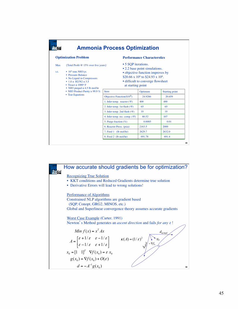
Hydrogen and Nitrogen feed are mixed, compressed, and combined with a recycle stream and heated to reactor temperature. Reaction occurs in a multibed reactor (modeled here as an equilibrium reactor) to partially convert the stream to ammonia. The reactor effluent is cooled and product is separated using two flash tanks with intercooling. Liquid from the second stage is flashed at low pressure to yield high purity NH3 product. Vapor from the two stage flash forms the recycle and is recompressed.
Ammonia Process Optimization
Hydrogen Feed Nitrogen Feed N2 5.2% 99.8% H2 94.0% --- CH4 0.79 % 0.02% Ar --- 0.01%
45
89
Optimization Problem Max {Total Profit @ 15% over five years}
s.t. • 105 tons NH3/yr. • Pressure Balance • No Liquid in Compressors • 1.8 ≤ H2/N2 ≤ 3.5
• Treact ≤ 1000o F • NH3 purged ≤ 4.5 lb mol/hr
• NH3 Product Purity ≥ 99.9 % • Tear Equations
Performance Characterstics
• 5 SQP iterations. • 2.2 base point simulations. • objective function improves by $20.66 x 10⁶ to $24.93 x 10⁶. • difficult to converge flowsheet at starting point
Item Optimum Starting point
Objective Function($106) 24.9286 20.659 1. Inlet temp. reactor (oF) 400 400 2. Inlet temp. 1st flash (oF) 65 65 3. Inlet temp. 2nd flash (oF) 35 35 4. Inlet temp. rec. comp. (oF) 80.52 107 5. Purge fraction (%) 0.0085 0.01 6. Reactor Press. (psia) 2163.5 2000 7. Feed 1 (lb mol/hr) 2629.7 2632.0 8. Feed 2 (lb mol/hr) 691.78 691.4
Ammonia Process Optimization
90
Recognizing True Solution • KKT conditions and Reduced Gradients determine true solution • Derivative Errors will lead to wrong solutions! Performance of Algorithms Constrained NLP algorithms are gradient based (SQP, Conopt, GRG2, MINOS, etc.) Global and Superlinear convergence theory assumes accurate gradients Worst Case Example (Carter, 1991) Newton’s Method generates an ascent direction and fails for any ε !
How accurate should gradients be for optimization?
)(
)()()( )( ]11[
/1/1/1/1
)(
01
00
000
xgAdOxfxg
xxfx
A
AxxxfMin
T
T
−−=
+∇=
=∇=
+−
−+=
=
ε
ε
εεεε
εεεε -g0
dactual
d idea
l
0f∇−
2)/1()( εκ =A
46
91
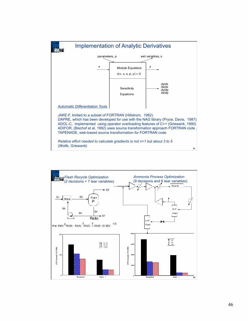
Implementation of Analytic Derivatives
Module Equations
c(v, x, s, p, y) = 0
Sensitivity
Equations
x y
parameters, p exit variables, s
dy/dxds/dxdy/dpds/dp
Automatic Differentiation Tools JAKE-F, limited to a subset of FORTRAN (Hillstrom, 1982) DAPRE, which has been developed for use with the NAG library (Pryce, Davis, 1987) ADOL-C, implemented using operator overloading features of C++ (Griewank, 1990) ADIFOR, (Bischof et al, 1992) uses source transformation approach FORTRAN code . TAPENADE, web-based source transformation for FORTRAN code Relative effort needed to calculate gradients is not n+1 but about 3 to 5 (Wolfe, Griewank)
92
S1 S2
S3
S7S4S5
S6
P
Ratio
M ax S3(A) *S3(B) - S3(A) - S3(C) + S3(D) - (S 3(E))2 2 3 1/2
M ix er Flas h
1 20
100
200
GRGSQPr SQP
Nu merical Exact
CPU
Sec
onds
(VS
3200
)
Flash Recycle Optimization
(2 decisions + 7 tear variables)
�
1 20
2000
4000
6000
8000
GRGSQPr SQP
Nu merical Exact
CPU
Sec
onds
(VS
3200
)
Reac tor
Hi P
Flas h
Lo P
Flas h
Ammonia Process Optimization
(9 decisions and 6 tear variables)
47
93
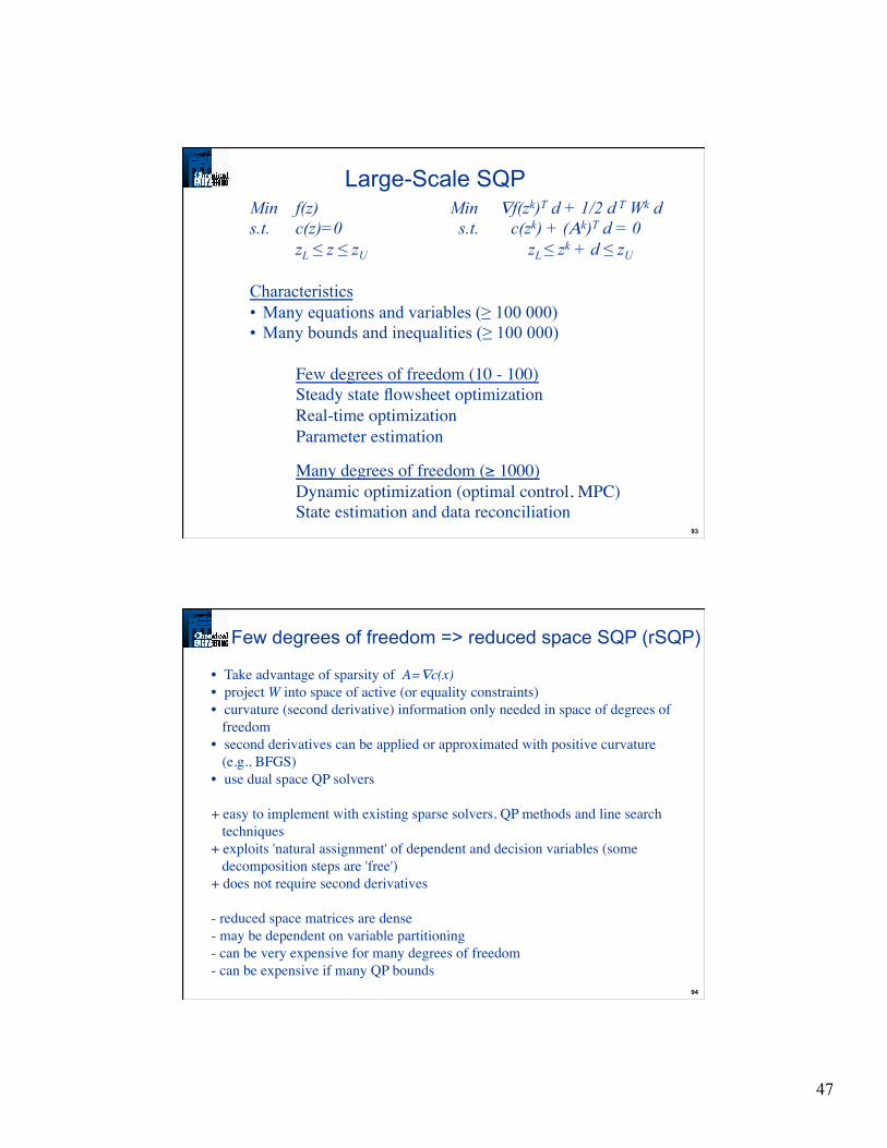
Min f(z) Min ∇f(zk)T d + 1/2 d T Wk d s.t. c(z)=0 s.t. c(zk) + (Αk)T d = 0 zL ≤ z ≤ zU zL ≤ zk + d ≤ zU
Characteristics
• Many equations and variables (≥ 100 000)
• Many bounds and inequalities (≥ 100 000)
Few degrees of freedom (10 - 100)
Steady state flowsheet optimization Real-time optimization
Parameter estimation
Many degrees of freedom (≥ 1000)
Dynamic optimization (optimal control, MPC)
State estimation and data reconciliation
Large-Scale SQP
94
• Take advantage of sparsity of A=∇c(x) • project W into space of active (or equality constraints) • curvature (second derivative) information only needed in space of degrees of freedom • second derivatives can be applied or approximated with positive curvature (e.g., BFGS) • use dual space QP solvers + easy to implement with existing sparse solvers, QP methods and line search techniques + exploits 'natural assignment' of dependent and decision variables (some decomposition steps are 'free') + does not require second derivatives - reduced space matrices are dense - may be dependent on variable partitioning - can be very expensive for many degrees of freedom - can be expensive if many QP bounds
Few degrees of freedom => reduced space SQP (rSQP)
48
95
�
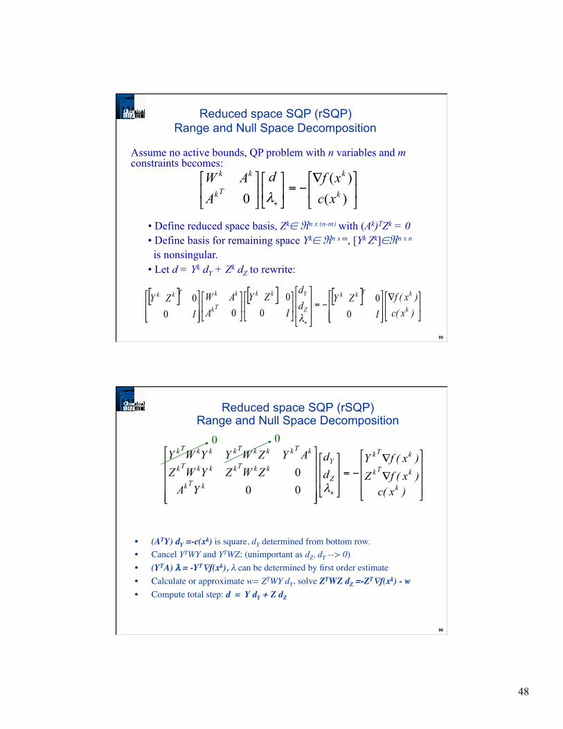
Reduced space SQP (rSQP) Range and Null Space Decomposition
∇−=
+ )()(
0 k
k
Tk
kk
xcxfd
AAW
λ
Assume no active bounds, QP problem with n variables and m constraints becomes:
• Define reduced space basis, Zk∈ ℜn x (n-m) with (Ak)TZk = 0 • Define basis for remaining space Yk∈ ℜn x m, [Yk Zk]∈ℜn x n is nonsingular. • Let d = Yk dY + Zk dZ to rewrite:
[ ] [ ] [ ]
∇
−=
+)x(c)x(f
IZY
dd
IZY
AAW
IZY
k
kTkk
Z
Ykk
Tk
kkTkk
00
00
000
λ
96
Reduced space SQP (rSQP) Range and Null Space Decomposition
• (ATY) dY =-c(xk) is square, dY determined from bottom row. • Cancel YTWY and YTWZ; (unimportant as dZ, dY --> 0) • (YTA) λ = -YT∇f(xk), λ can be determined by first order estimate • Calculate or approximate w= ZTWY dY, solve ZTWZ dZ =-ZT∇f(xk) - w • Compute total step: d = Y dY + Z dZ
∇
∇−=
+ )x(c)x(fZ)x(fY
dd
YAZWZYWZ
AYZWYYWY
k
kTk
kTk
Z
Y
kTk
kkTkkkTk
kTkkkTkkkTk
λ000
0 0
49
97
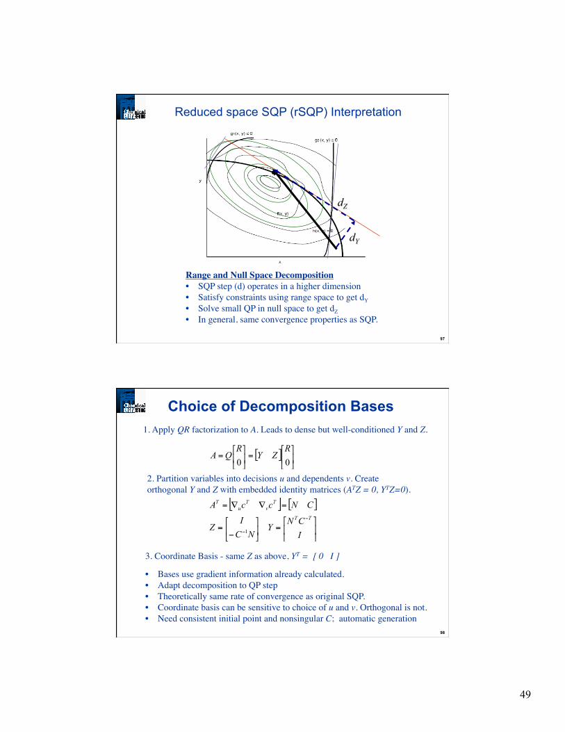
Range and Null Space Decomposition • SQP step (d) operates in a higher dimension • Satisfy constraints using range space to get dY • Solve small QP in null space to get dZ • In general, same convergence properties as SQP.
Reduced space SQP (rSQP) Interpretation
dY
dZ
98
1. Apply QR factorization to A. Leads to dense but well-conditioned Y and Z.
2. Partition variables into decisions u and dependents v. Create orthogonal Y and Z with embedded identity matrices (ATZ = 0, YTZ=0).
3. Coordinate Basis - same Z as above, YT = [ 0 I ]
• Bases use gradient information already calculated. • Adapt decomposition to QP step
• Theoretically same rate of convergence as original SQP. • Coordinate basis can be sensitive to choice of u and v. Orthogonal is not. • Need consistent initial point and nonsingular C; automatic generation
Choice of Decomposition Bases
[ ]
=
=
00R
ZYR
QA
[ ] [ ]
=
−=
=∇∇=−
− ICN
YNC
IZ
CNccATT
Tv
Tu
T
1
50
99
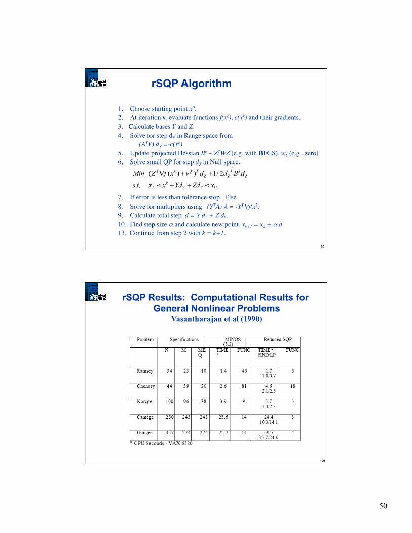
1. Choose starting point x0. 2. At iteration k, evaluate functions f(xk), c(xk) and their gradients. 3. Calculate bases Y and Z. 4. Solve for step dY in Range space from (ATY) dY =-c(xk)
5. Update projected Hessian Bk ~ ZTWZ (e.g. with BFGS), wk (e.g., zero) 6. Solve small QP for step dZ in Null space.
7. If error is less than tolerance stop. Else 8. Solve for multipliers using (YTA) λ = -YT∇f(xk) 9. Calculate total step d = Y dY + Z dZ. 10. Find step size α and calculate new point, xk+1 = xk + α d 13. Continue from step 2 with k = k+1.
rSQP Algorithm
UZYk
L
ZkT
ZZTkkT
xZdYdxxtsdBddwxfZMin
≤++≤
++∇
..
2/1))((
100
rSQP Results: Computational Results for General Nonlinear Problems
Vasantharajan et al (1990)

51
101
rSQP Results: Computational Results for Process Problems Vasantharajan et al (1990)
102
Coupled Distillation Example - 5000 Equations Decision Variables - boilup rate, reflux ratio Method CPU Time Annual Savings Comments
1. SQP* 2 hr negligible Base Case 2. rSQP 15 min. $ 42,000 Base Case 3. rSQP 15 min. $ 84,000 Higher Feed Tray Location 4. rSQP 15 min. $ 84,000 Column 2 Overhead to Storage 5. rSQP 15 min $107,000 Cases 3 and 4 together
18
10
1
QVKQVK
Comparison of SQP and rSQP
52
103
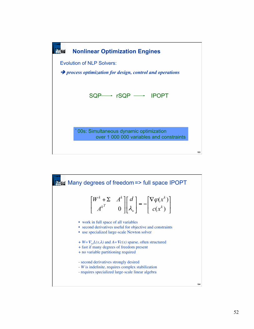
Nonlinear Optimization Engines
Evolution of NLP Solvers:
process optimization for design, control and operations
’80s: Flowsheet optimization over 100 variables and constraints ‘90s: Static Real-time optimization (RTO) over 100 000 variables and constraints ’00s: Simultaneous dynamic optimization over 1 000 000 variables and constraints
SQP rSQP IPOPT
104
Many degrees of freedom => full space IPOPT
• work in full space of all variables • second derivatives useful for objective and constraints • use specialized large-scale Newton solver + W=∇xxL(x,λ) and A=∇c(x) sparse, often structured + fast if many degrees of freedom present + no variable partitioning required - second derivatives strongly desired - W is indefinite, requires complex stabilization - requires specialized large-scale linear algebra
∇−=
Σ+
+ )()(
0 k
k
Tk
kk
xcxd
AAW ϕ
λ
53
105
GAS STATIONS
Final Product tanks
Supply tanks
Intermediate tanks
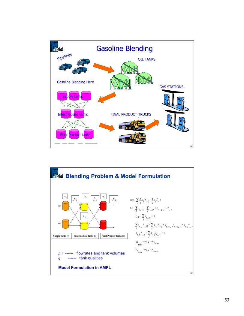
Gasoline Blending Here
Gasoline Blending OIL TANKS Pipelines
FINAL PRODUCT TRUCKS
106
Blending Problem & Model Formulation
⇒
⇒
Final Product tanks (k) Intermediate tanks (j) Supply tanks (i)
ijtf , jktf ,
jtv ,
itq ,
iq
jtq ,.. ktq ,.. kv
ktf ,..
f, v ------ flowrates and tank volumes q ------ tank qualities
Model Formulation in AMPL
max ,
min
max ,
min
0,,,,
,,,1,1,,,,
0,,
,,1,, s.t.
)t ,
( , max
jvjtvjv
kqktqkq
j jktfjt
qkt
fkt
q
jtvjt
qjt
vjt
qi ijt
fit
qk jkt
fjt
q
j jktfktf
jtv
jtv
i ijtf
k jktf
i ic
ktf
k kc itf
≤≤
≤≤
=−
=++
+−
=−
=+
+−
∑−∑
∑
∑∑
∑
∑∑
∑
54
107
F1
F2
F3
P1
B1
B2
F1
F2
F3
P2
P1
B1
B2
B3
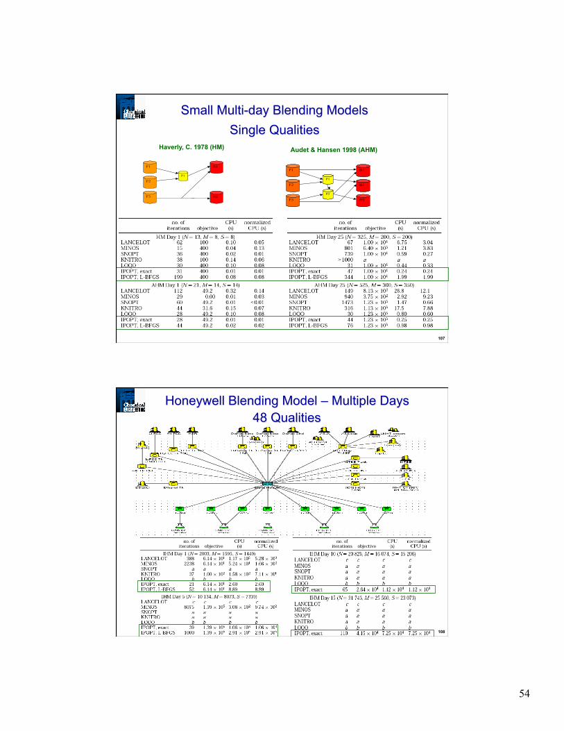
Haverly, C. 1978 (HM) Audet & Hansen 1998 (AHM)
Small Multi-day Blending Models Single Qualities
108
Honeywell Blending Model – Multiple Days 48 Qualities
55
109
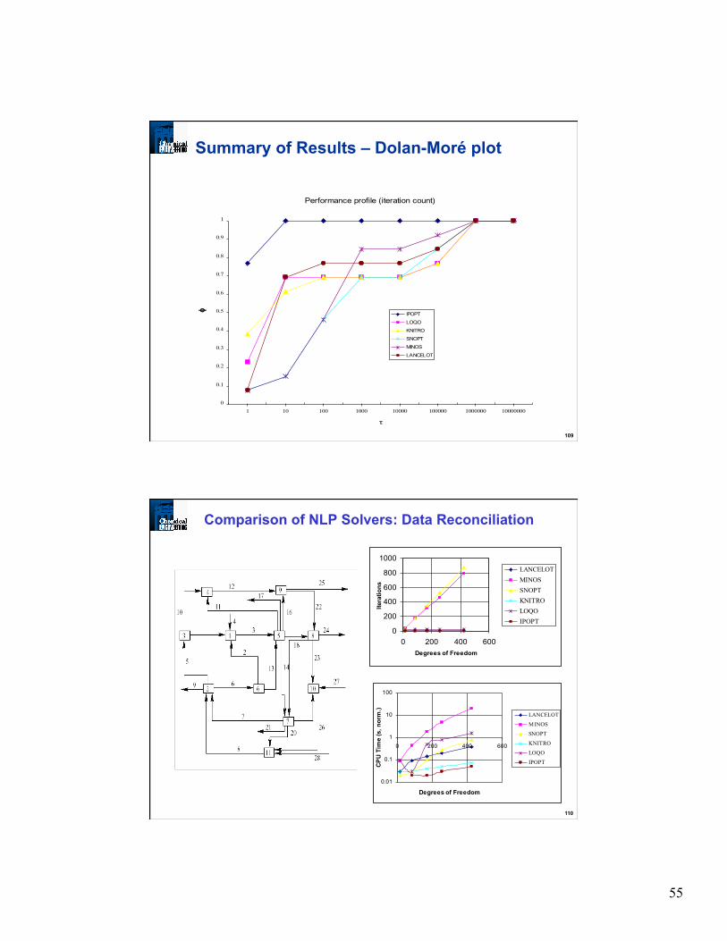
Summary of Results – Dolan-Moré plot
Performance profile (iteration count)
0
0.1
0.2
0.3
0.4
0.5
0.6
0.7
0.8
0.9
1
1 10 100 1000 10000 100000 1000000 10000000
τ
φ
IPOPT
LOQO
KNITRO
SNOPT
MINOS
LANCELOT
110
Comparison of NLP Solvers: Data Reconciliation
0.01
0.1
1
10
100
0 200 400 600
Degrees of Freedom
CPU
Tim
e (s
, nor
m.)
LANCELOT
MINOS
SNOPT
KNITRO
LOQO
IPOPT
0
200
400
600
800
1000
0 200 400 600Degrees of Freedom
Itera
tions
LANCELOTMINOSSNOPTKNITROLOQOIPOPT

56
111
Comparison of NLP solvers (latest Mittelmann study)
117 Large-scale Test Problems
500 - 250 000 variables, 0 – 250 000 constraints
Mittelmann NLP benchmark (10-26-2008)
0
0.1
0.2
0.3
0.4
0.5
0.6
0.7
0.8
0.9
1
0 2 4 6 8 10 12
log(2)*minimum CPU time
fract
ion
solve
d wi
thin
IPOPTKNITROLOQOSNOPTCONOPT
Limits Fail IPOPT 7 2 KNITRO 7 0 LOQO 23 4 SNOPT 56 11 CONOPT 55 11
112
Typical NLP algorithms and software
SQP - NPSOL, VF02AD, NLPQL, fmincon
reduced SQP - SNOPT, rSQP, MUSCOD, DMO, LSSOL…
Reduced Grad. rest. - GRG2, GINO, SOLVER, CONOPT
Reduced Grad no rest. - MINOS
Second derivatives and barrier - IPOPT, KNITRO, LOQO
Interesting hybrids -
• FSQP/cFSQP - SQP and constraint elimination
• LANCELOT (Augmented Lagrangian w/ Gradient Projection)

57
113
Optimization Algorithms -Unconstrained Newton and Quasi Newton Methods -KKT Conditions and Specialized Methods -Reduced Gradient Methods (GRG2, MINOS) -Successive Quadratic Programming (SQP) -Reduced Hessian SQP -Interior Point NLP (IPOPT) Process Optimization Applications -Modular Flowsheet Optimization -Equation Oriented Models and Optimization -Realtime Process Optimization -Blending with many degrees of freedom Further Applications -Sensitivity Analysis for NLP Solutions -Multi-Scenario Optimization Problems
Summary and Conclusions