nonlinear pulse propagation
TRANSCRIPT

ETH ZurichUltrafast Laser Physics
Ursula Keller / Lukas Gallmann
ETH Zurich, Physics Department, Switzerlandwww.ulp.ethz.ch
Chapter 4: Nonlinear pulse propagation
Ultrafast Laser Physics

Kerr effect and self-phase modulation (SPM)
n I( ) = n + n2 I n2cm2
W⎡
⎣⎢
⎤
⎦⎥ = 4.19 ×10
−3 n2 esu[ ]n
Material Refractive index n n2 esu[ ] n2 cm2 / W⎡⎣ ⎤⎦
Sapphire (Al2O3) 1.76 @ 850 nm 1.25 ×10⁻¹³ [89Ada] 3×10⁻¹⁶ Fused quartz 1.45 @ 1.06 m 0.85 ×10⁻¹³ [89Ada] 2.46 ×10⁻¹⁶ Glass (Schott LG-760) 1.5 @ 1.06 m 1.04 ×10⁻¹³ [93Aza] 2.9 ×10⁻¹⁶
YAG (Y3Al5O12) 1.82 @ 1.064 m 3.47 ×10⁻¹³ [93Aza] 6.2 ×10⁻¹⁶
YLF (LiYF4) ne = 1.47@ 1.047 m
1.72 ×10⁻¹⁶ [93Aza]
ULP, Chap. 4, p. 1
Typical order of magnitude for the nonlinear index coefficient: n2 ≈ 10–16 cm2/W
Self-phase modulation (SPM):
SPM coefficient:
φ t( ) = −kn I( )LK = −k n + n2 I t( )⎡⎣ ⎤⎦ LK
δ ≡ kn2LK
φ2 t( ) = −kn2 I t( )LK = −kn2LK A t( ) 2 ≡ −δ A t( ) 2

Kerr effect and self-phase modulation (SPM)
ULP, Chap. 4, p. 2
t
I(t)
Zeitabhängige Intensität
tω0
ω ( t)
Verbreiterung des Spektrums
Pulsfront
Pulsflanke
2
Gaussian Pulse
Spectral broadening
leading edgeSPM: red
trailing edgeSPM: blue
I t( )
t
t
ω2 t( )
ω0
ω2 t( ) = dφ2 t( )dt
= −δdI t( )dt
φ2 t( ) = −kn2 I t( )LK = −kn2LK A t( ) 2 ≡ −δ A t( ) 2
δ ≡ kn2LK
Spectral broadening of a transform-limited pulse:
“red before blue”
n2 > 0

Number of oscillations in SPM-broadened spectrum
ULP, Chap. 4, p. 3
φ2,max = kn2I pLK ≈ M −12
⎛⎝⎜
⎞⎠⎟π
Theory: Parameter Experiment: Gaussian pulse in 99 mfiber.
R. H. Stolen, C. Lin, Phys. Rev. A, 17, 1448, 1978
φ2,max

SPM• Instantaneous change of refractive index:
• Consequences for a sech2 pulse (without dispersion):
• Small phase changes: weak spectral broadening; approximately parabolic phase in frequency domain(can be compensated by constant GDD!)
• Large phase changes:complicated spectralbroadening(complete compressionis difficult)
4
2
0
-2
-4-400 -200 0 200 400
frequency offset (GHz)
intensity (a. u.)phase (rad)
2( ) ( )n t n I tΔ =

Pure SPM in the Wigner picture
• Temporal pulse shape remains unchanged• Spectrum broadens• Oscillatory spectral features due to interference in frequency domain
Initially 10 fs long Gaussian pulse at 800 nm, SPM (n2>0) only
n I( ) = n + n2 I

Comparison with effect of TODEverything calculated for an initially 10-fs long Gaussian pulse
After 1000 fs3 of TOD:
ϕ(ω ) = 16⋅1000 fs3 ⋅ ω −ω 0( )3
• “Beating of simultaneous frequencies”causes post-(pre-)pulses
• Interference in time domain

Comparison of SPM and GDDEverything calculated for an initially 10-fs long Gaussian pulse
After 100 fs2 of GDD:
ϕ(ω ) = 12⋅100 fs2 ⋅ ω −ω 0( )2
• “Red” before “blue”
• Chirp is (mostly) linear in center
After SPM (n2>0):
φ2 t( ) = −kn2 I t( )LK = −kn2LK A t( ) 2 ≡ −δ A t( ) 2
⇒ Negative GDD can compensate linear chirp in center of SPM broadened pulse

Fiber grating pulse compressor
ULP, Chap. 4, p. 4

World-record pulse duration in 1987
Fiber-grating-prism-pulse compressor for the compression of 50 fs to 6 fs at 8 kHzcenter wavelength 620 nm
SPM broadened spectrum: quartz fiber with core diameter of ≈ 4 µm and a length of 0.9 cm, peak intensity 1-2 x 10¹² W/cm2
Measured interferometric autocorrelation
6 fs FWHM
ULP, Chap. 4, p. 5

World-record pulse duration in 1999
ULP, Chap. 4, p. 5
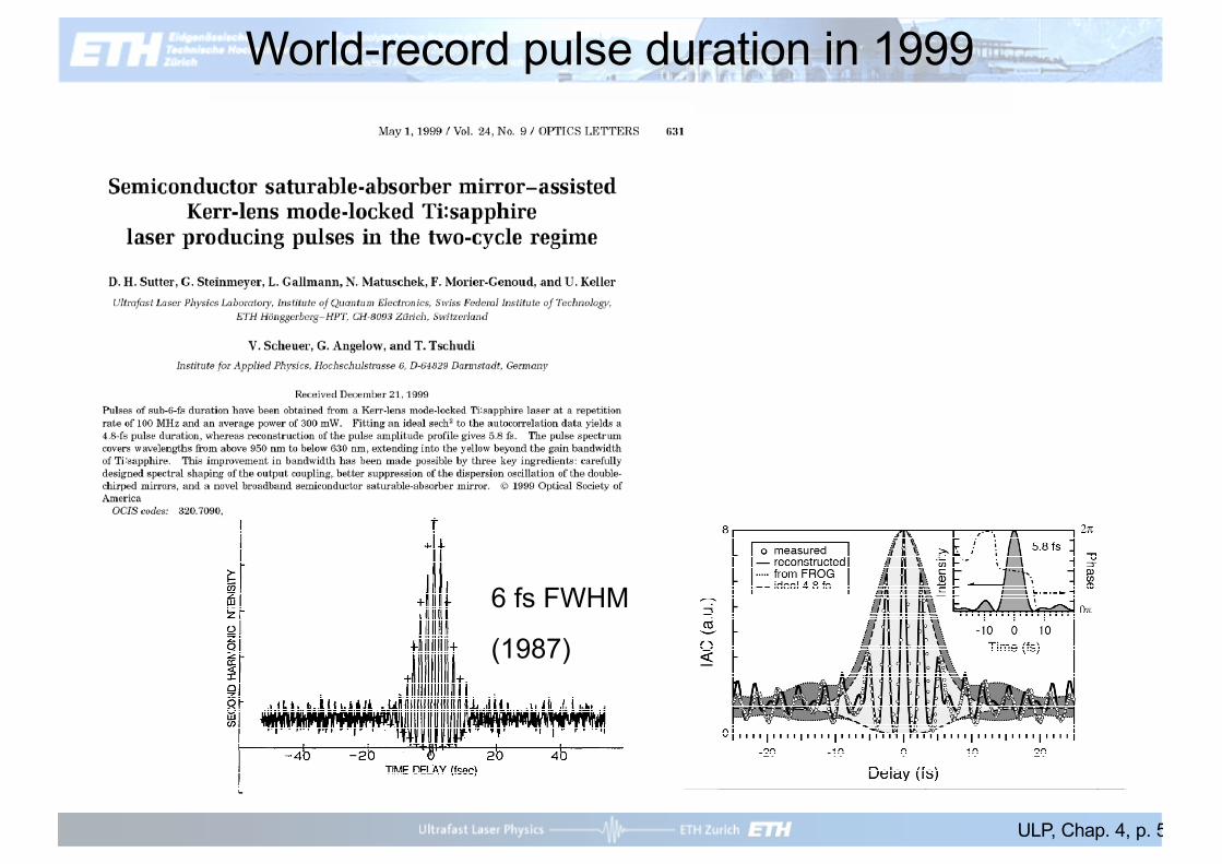
World-record pulse duration in 1999
6 fs FWHM
(1987)
ULP, Chap. 4, p. 5

Compressed pulses from a thin-disk laser
After compressionPavg = 32 Wτ p = 24 fs
After fiberPavg = 42 Wlaunch efficiency: 70%Prej = 10 W (PBS)
Incident on fiberPavg = 60 Wτ p = 760 fsIpeak = 1.2 TW/cm2
ASSP 2005
ULP, Chap. 4, p. 6

large mode area fiber
Aeff≈ 200 µm2 (mode area)d ≈ 2.7µm (hole Ø)Λ ≈ 11 µm (spacing)
T. Südmeyer, et al., Opt. Lett. 28, 1951 (2003) and E. Innerhofer, TuA3, ASSP 2004ORC Southampton
After compressionPavg = 32 WEp = 0.56 μJτp = 24 fsPpeak = 16 MW
Incident on fiberPavg = 60 WEp ≈ 1 μJτp = 760 fsIpeak = 1.2 TW/cm2
but fiber damage after 10-20 minutes
Compressed pulses from a thin-disk laser

autocorrelation
optical spectrum (not symmetric - other nonlinearities, self-steepening)
retrieved pulse
Compression outputPavg = 32 W frep = 57 MHzPpeak = 16 MW τp = 24 fsEp= 0.56 µJ• 73% of energy in central pulse• Fourier limit: 20 fs• fiber damage after ≈ 15 minutes
ASSP 2005ULP, Chap. 4, p. 6
Compressed pulses from a thin-disk laser

Nonlinear pulse compression
100 µm
Microstructured fiber withlarge mode area
Used fiber:#
effektive mode area ≈ 205 µm2
# K. Furusawa, J. C. Baggett, T. M. Monro, and D. J. Richardson, ORC Southampton
• Approach: SPM in a fiber for spectral broadening, grating or prisms for dispersion compensation
• Established technique, but used for much lower power• High power in fiber requires large mode area with single-mode
operation

−2000 −1200 −400 400 1200 20000
102030405060708090
100110
peak
pow
er /
MW
Delay / fs
−2000 −1200 −400 400 1200 20000481216202428323640
spec
tral p
hase
/ ra
d
retrieved pulse
88 fs
Nonlinear compression (in gas-filled hollow fiber) Fiber (7-cell 3-ring hypocycloid core designed for 1030 nm)mode diameter: 30 µm length: 66 cm filling: 13 bar Argon
Compressed output
Pav = 112 Wτp = 88 fsPpeak = 105 MWfrep = 7 MHzEp = 16 µJMain Peak = 59%
T = 92% T > 95% T > 99.7%
Total equivalent efficiency > 88%Laser input
Pav = up to 127 Wτp = 740 fsPpeak = 21 MWfrep = 7 MHzEp = 18 µJ
20 bounces
≈ - 11 kfs2 of dispersion
F. Emaury et al., Opt. Lett. 39, 6843 (2014)

Fiber compressor for 5.5 fs pulses
SPIDER
Ti:Sa
SLM
G GSM SM
OCDCMsAS ASMF
15 fs, 16 nJ
0.2nJ
SPM broadening in a microstructure fiber (MF), length 5 mm
Ti:sapphire laser with prism pair and DCMs: frep = 19 MHz (for higher pulse energy)
Microstructure fiber (MF):2.6 µm core diameter5 mm longzero GDD at 940 nm
B. Schenkel et al., JOSA B 22, 687, 2005
1.0
0.5
0.0
Inte
nsity
(a. u
.)
1000750500Wavelength (nm)
-600
-400
-200
0
Dis
pers
ion
(ps/
nm/k
m)

Broadband pulse shaper with SLM
Possible bandwidth through Spatial Light Modulator: 400 - 1050 nm
SLM640 pixels
300 l/mm grating 300 l/mm grating
f = 300 mm f = 300 mm
knife-edge
A. M. Weiner, Rev. Sci. Instrum. 71, 1929 (2000)spatial light modulator (640 pixel liquid crystal, each pixel ≈100 µm wide, 3 µm gap)

1.0
0.5
0.0
Inte
rfer
ogra
m
420370320Wavelength (nm)
1.0
0.5
0.0
Inte
nsity
(a. u
.)
-40 -20 0 20 40Time (fs)
5.5 fs
• Good fringe visibility: reliable SPIDER measurement
• Microstructure fiber 2.6-µm corediameter, 5 mm long, zero GDDat 940 nm
1.0
0.5
0.0Pow
er d
ensi
ty (a
. u.)
1000750500Wavelength (nm)
-4
0
4
Spec
tral
pha
se (r
ad)
5.5 fs, 0.2 nJ
Fiber compressor for 5.5 fs pulses
B. Schenkel et al., JOSA B 22, 687, 2005
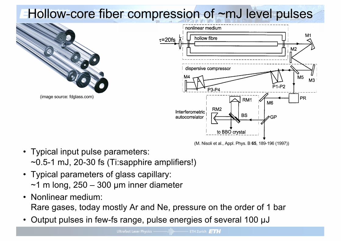
Hollow-core fiber compression of ~mJ level pulses
(image source: fdglass.com)
(M. Nisoli et al., Appl. Phys. B 65, 189-196 (1997))
• Typical input pulse parameters:~0.5-1 mJ, 20-30 fs (Ti:sapphire amplifiers!)
• Typical parameters of glass capillary:~1 m long, 250 – 300 µm inner diameter
• Nonlinear medium:Rare gases, today mostly Ar and Ne, pressure on the order of 1 bar
• Output pulses in few-fs range, pulse energies of several 100 µJ

Dual stage hollow fiber compressor for 3.8 fs
SPIDER
Ti:Sa Amp
continuum generation
25 fs, 0.5 mJ
100 µJ
15 µJShaper
B. Schenkel et al.: Opt. Lett. 28, 1987 (2003)

Dual stage hollow fiber compressor for 3.8 fs
3.8 fs, 15 µJ
2π phase shift→ pre- and post-pulses
1.0
0.5
0.0Sp
ectr
al P
ow
er D
ensi
ty
1000750500Wavelength (nm)
-4
-2
0
2
4
Sp
ectr
al P
has
e (r
ad)1.0
0.5
0.0
Inte
rfer
ogra
m
460400340Wavelength (nm)
1.0
0.5
0.0
Inte
nsity
-40 -20 0 20 40Time (fs)
3.8 fs
B. Schenkel et al.: Opt. Lett. 28, 1987 (2003)

Choice of compression medium• Available input pulse parameters determine best medium for pulse
compression• Limits peak power: bulk damage due to self-focusing (see next slides)• However, damage in fibers usually occurs at facets first ⇒ Want highest available nonlinearity without damage
Pulse energy pJ-nJ multi-nJ µJ mJ
Peak power <MW MW 10s-100s of MW GW
Nonlinearity few 10-16 cm2/W few 10-16 cm2/W few 10-19 cm2/W few 10-19 cm2/W
Mode size ~µm ~10 µm 10s of µm 100s of µm
Medium Microstructure fiber
Standard fiber Hollow micro-structure fiber
Hollow-core fiber (capillary)
• Not much choice with regards to compression medium• Compression of femtosecond pulses with more than a few mJ is very
challenging

Optical pulse cleaner
Optical pulse cleaner based on nonlinear birefringenceOptics Letters, vol. 17, pp. 136-138, 1992
ULP, Chap. 4, p. 9-10

Self-focusing
Kerr mediumlength LK
n x,y( ) = n + n2 I x,y( )
≅ np − 2Δnpx2 + y2
w2
f = w2
4ΔnpLK
I x,y( ) = I pexp −2 x2 + y2
w2
⎛⎝⎜
⎞⎠⎟
↓ x2 + y2( ) << w2
≈ I p 1− 2 x2 + y2
w2
⎛⎝⎜
⎞⎠⎟
ULP, Chap. 4, p. 11

B-integral
ULP, Chap. 4, p. 10
B ≡ 2πλ
n2 I z( )dz0
L
∫
To prevent material damage: B should be smaller than 3 to 5

Critical power for beam collapse
ULP, Chap. 4, p. 14
Pcr ≡ 3.72λ02 / 8π n0n2
Lc =0.376LDF
Pin / Pcr( )1 2 − 0.852⎡⎣
⎤⎦2 − 0.0219
LDF = π n0w02
λ0Rayleigh length
Lc
Argon at 800 nm (atmospheric pressure):
n0 = 1.0, n2 = 3 10–19 cm2/W, Pcr = 3.2 GW
Fused quartz at 1.06 µm:
n0 = 1.45, n2 = 2.46 10–16 cm2/W, Pcr = 3.8 MW

Filamentation
ULP, Chap. 4, p. 14

Filamentation
During propagation SPM continues to broaden spectrum of pulse ⇒ white light
Filamentation of mJ-level, 30-fs pulses at 800 nm in Ar

Filamentation pulse compression
660 μJ
900 mbar340 μJ
820 mbar
120 μJ
30 fs
10 fs
5 fs
A. Guandalini et al., J. Phys. B 39, S257 (2006)C.P. Hauri et al., Opt. Exp. 13, 7541 (2005)

Comparison with hollow-core fiber
Filamentation• SPM and plasma generation• Self-compression possible• Beam is spatially less
homogeneous (spatio-temporal coupling)
• More robust to beam pointing fluctuations at input
• More instability of beam pointing at output
Hollow-core fiber• SPM is dominant nonlinear
process• Self-compression typically not
possible• Capillary acts as spatial filter,
homogenizes output• Sensitive to in-coupling of beam
0.001
2
46
0.01
2
46
0.1
2
46
1
Spec
trum
900800700600500Wavelength (nm)
Hollow core-fiber Filament
1.0
0.8
0.6
0.4
0.2
0.0
Spec
trum
900800700600500W avelength (nm)
Hollow core-fiber Filament
(L. Gallmann et al., Appl. Phys. B 86, 561 (2007))

Fundamental Soliton Pulses• Basic idea: nonlinear phase change from Kerr effect is
compensated by dispersive phase change,apart from a constant phase shift.
• Conditions (for constant GDD):
• Negative (anomalous) GDD, if n2 > 0
• Unchirped sech2 pulse shape, fulfilling the condition
• Remarkable stability of soliton pulses:
particle character in collision
pulse automatically “finds“ the exact required shape (may shed some energy into a background pulse)
τ p = 1.7627 ×4 Dδ ep
= 1.7627 ×2 ′′kn kn2ep

Nonlinear pulse propagation Linear pulse propagation:GDD and no SPM
Nonlinear pulse propagation:no GDD and SPM
′′kn ≠ 0
n2 = 0
′′kn = 0
n2 ≠ 0
ULP, Chap. 4, p. 18

Nonlinear pulse propagation Nonlinear pulse propagation: GDD > 0 and SPM > 0
Nonlinear pulse propagation:Soliton pulsesGDD < 0 and SPM > 0
ULP, Chap. 4, p. 19
′′kn > 0
n2 > 0
n2 > 0
′′kn < 0

Nonlinear Schrödinger Equation (NSE)
ULP, Chap. 4, p. 15
Slowly varying envelope approximation:
Dispersion first order:Linearized operator in the time domain
A Ld ,Δω( ) = e− i kn ω0+Δω( )−kn ω0( )⎡⎣ ⎤⎦Ld A(0,Δω )
kn ω( ) ≅ kn ω0( ) + ′knΔω + 12
′′knΔω2
′kn =∂kn∂ω ω0
′′kn =∂ 2kn∂ω 2
ω0
A Ld ,Δω( ) = exp −i ′knΔω + 12
′′knΔω2⎛
⎝⎜⎞⎠⎟ Ld
⎧⎨⎩
⎫⎬⎭A(0,Δω )
′knΔωLd << 1
A Ld ,Δω( ) = e− i ′knΔωLd A 0,Δω( ) ≅ 1− i ′knΔωLd( ) A 0,Δω( )
F−1 Δω A z,Δω( ){ } = −i ∂
∂tA z,t( )
A Ld ,t( ) ≅ 1− ′kn Ld∂∂t
⎛⎝⎜
⎞⎠⎟ A 0,t( ) , for ′knΔωLd << 1

Nonlinear Schrödinger Equation (NSE)
ULP, Chap. 4, p. 16
Slowly varying envelope approximation:
Dispersion second order:Linearized operator in the time domain
Dispersion parameter D
A Ld ,Δω( ) = e− i kn ω0+Δω( )−kn ω0( )⎡⎣ ⎤⎦Ld A(0,Δω )
kn ω( ) ≅ kn ω0( ) + ′knΔω + 12
′′knΔω2
′kn =∂kn∂ω ω0
′′kn =∂ 2kn∂ω 2
ω0
A Ld ,Δω( ) = exp −i ′knΔω + 12
′′knΔω2⎛
⎝⎜⎞⎠⎟ Ld
⎧⎨⎩
⎫⎬⎭A(0,Δω )
F−1 Δω 2 A z,Δω( ){ } = − ∂ 2
∂t 2A z,t( )
′′knΔω2Ld << 1
A Ld ,Δω( ) = e− i
12
′′knΔω2Ld A 0,Δω( ) ≅ 1− i 1
2′′knΔω
2Ld⎛⎝⎜
⎞⎠⎟A 0,Δω( )
A Ld ,t( ) ≅ 1+ i 12
′′kn Ld∂ 2
∂t 2⎛⎝⎜
⎞⎠⎟
A 0,t( ) ≡ 1+ iD ∂ 2
∂t 2⎛⎝⎜
⎞⎠⎟
A 0,t( ) , for ′′knΔω2Ld << 1D ≡ 1
2′′knLd

Nonlinear Schrödinger Equation (NSE)
ULP, Chap. 4, p. 17
A Ld ,t( ) ≅ 1+ i 12
′′kn Ld∂ 2
∂t 2⎛⎝⎜
⎞⎠⎟
A 0,t( ) ≡ 1+ iD ∂ 2
∂t 2⎛⎝⎜
⎞⎠⎟
A 0,t( ) , for ′′knΔω2Ld << 1
A Ld ,t( ) ≅ 1− ′kn Ld∂∂t
⎛⎝⎜
⎞⎠⎟ A 0,t( ) , for ′knΔωLd << 1 1. Order Dispersion
2. Order Dispersion
∂∂z
A z,t( ) = limLd→0
A Ld ,t( ) − A 0,t( )Ld
≈ − ′kn∂∂tA z,t( ) + i 1
2′′kn∂ 2
∂t 2A z,t( )
∂∂z
A z,t( ) + 1υg
∂∂tA z,t( ) = i ′′kn
2∂ 2
∂t 2A z,t( )
∂∂z
A z, ′t( ) = i ′′kn2
∂ 2
∂ ′t 2A z, ′t( )
′t = t − zυg
retarded time

SPM operator
ULP, Chap. 4, p. 2
E LK ,t( ) = A 0,t( )exp iω0t + iφ t( )⎡⎣ ⎤⎦ = A 0,t( )exp iω0t − ikn ω0( )LK − iδ A t( ) 2⎡⎣
⎤⎦
A LK ,t( ) = e− iδ A 2
A 0,t( )e− ikn ω0( )LK δ A 2<<1⎯ →⎯⎯⎯ ≈ 1− iδ A t( ) 2( )A 0,t( )e− ikn ω0( )LK
SPM Operator (linearized)
δ ≡ kn2LK
δ A t( ) 2 = δ I t( ) << 1

Nonlinear Schrödinger Equation (NSE)
ULP, Chap. 4, p. 17
A Ld ,t( ) ≅ 1+ i 12
′′kn Ld∂ 2
∂t 2⎛⎝⎜
⎞⎠⎟
A 0,t( ) ≡ 1+ iD ∂ 2
∂t 2⎛⎝⎜
⎞⎠⎟
A 0,t( ) , for ′′knΔω2Ld << 1
A Ld ,t( ) ≅ 1− ′kn Ld∂∂t
⎛⎝⎜
⎞⎠⎟ A 0,t( ) , for ′knΔωLd << 1 1. Order Dispersion
2. Order Dispersion
∂∂z
A z,t( ) = limLd→0
A Ld ,t( ) − A 0,t( )Ld
≈ − ′kn∂∂tA z,t( ) + i 1
2′′kn∂ 2
∂t 2A z,t( )
′t = t − zυg
retarded time
A LK ,t( ) ≈ 1− iδ A t( ) 2( )A 0,t( ) δ ≡ kn2LK
∂∂z
A z,t( ) = limLd→0
A L,t( ) − A 0,t( )L
≈ − ′kn∂∂tA z,t( ) + i 1
2′′kn∂ 2
∂t 2A z,t( ) − ikn2 A t( ) 2 A z,t( )
+ SPM
∂∂z
A z, ′t( ) = i ′′kn2
∂ 2
∂ ′t 2A z, ′t( ) − ikn2 A z, ′t( ) 2 A z, ′t( ) Nonlinear Schrödinger Equation (NSE)

Nonlinear Schrödinger Equation (NSE)
∂∂z
A z, ′t( ) = i ′′kn2
∂ 2
∂ ′t 2A z, ′t( ) − ikn2 A z, ′t( ) 2 A z, ′t( ) Nonlinear Schrödinger Equation (NSE)
As z, ′t( ) = A0sech′tτ
⎛⎝⎜
⎞⎠⎟ e− iφ0
τ p = 1.7627 ⋅τ
Δν pτ p = 0.3148
Solution: a fundamental soliton
φ0 =φ2max2
φ2max = kn2 I pz , I p = A02
The pulse as a whole experiences a homogeneousphase shift (not like SPM alone!)
ULP, Chap. 4, p. 20

Nonlinear Schrödinger Equation (NSE)
∂∂z
A z, ′t( ) = i ′′kn2
∂ 2
∂ ′t 2A z, ′t( ) − ikn2 A z, ′t( ) 2 A z, ′t( ) Nonlinear Schrödinger Equation (NSE)
As z, ′t( ) = A0sech′tτ
⎛⎝⎜
⎞⎠⎟ e− iφ0
τ p = 1.7627 ⋅τ
Δν pτ p = 0.3148
Solution: a fundamental soliton
φ0 =φ2max2
φ2max = kn2 I pz , I p = A02
The pulse as a whole experiences a homogeneousphase shift (not like SPM alone!)
ULP, Chap. 4, p. 21
τ p = 1.7627 ×4 Dδ ep
= 1.7627 ×2 ′′kn kn2ep
∝ 1ep

Nonlinear Schrödinger Equation (NSE)
∂∂z
A z, ′t( ) = i ′′kn2
∂ 2
∂ ′t 2A z, ′t( ) − ikn2 A z, ′t( ) 2 A z, ′t( ) Nonlinear Schrödinger Equation (NSE)
As z, ′t( ) = A0sech′tτ
⎛⎝⎜
⎞⎠⎟ e− iφ0
τ p = 1.7627 ⋅τ
Δν pτ p = 0.3148
Solution: a fundamental soliton
φ0 =φ2max2
φ2max = kn2 I pz , I p = A02
The pulse as a whole experiences a homogeneousphase shift (not like SPM alone!)
ULP, Chap. 4, p. 21
Balance between negative GDD and positive SPM:
φ0 =Dτ 2
= 12δ I p =
δ ep
4τ=
kn2 ep
4τz
δ ≡ kn2LK D ≡ 12
′′knLd
ep =Ep
Aeff= I z, ′t( )∫ d ′t = As z, ′t( ) 2 d ′t∫ = 2 A0
2 τ
τ p = 1.7627 ×4 Dδ ep
= 1.7627 ×2 ′′kn kn2ep
∝ 1ep
Nonlinear Schrödinger Equation (NSE)
∂∂z
A z, ′t( ) = i ′′kn2
∂ 2
∂ ′t 2A z, ′t( ) − ikn2 A z, ′t( ) 2 A z, ′t( ) Nonlinear Schrödinger Equation (NSE)
Solution: a fundamental soliton
ULP, Chap. 4, p. 22
τ p = 1.7627 ×4 Dδ ep
= 1.7627 ×2 ′′kn kn2ep
∝ 1ep
τ p ∝1ep
τ p ∝ ′′kn
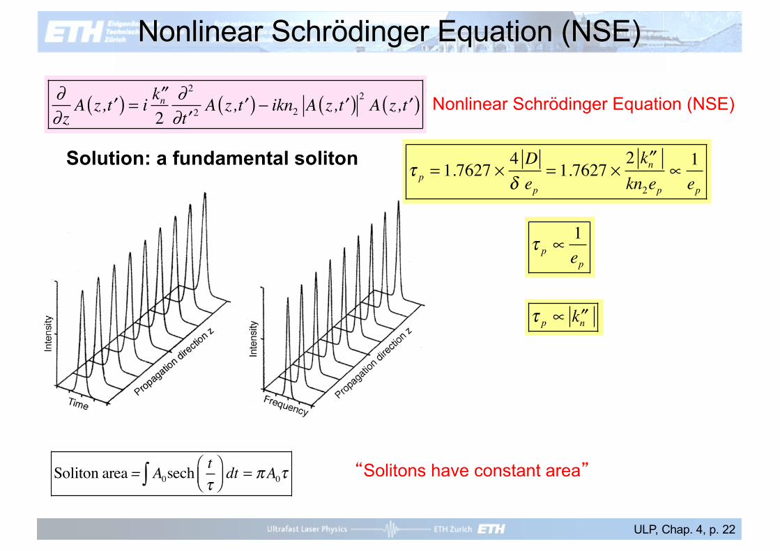
Soliton area = A0∫ sech tτ
⎛⎝⎜
⎞⎠⎟ dt = πA0τ “Solitons have constant area”
Nonlinear Schrödinger Equation (NSE)
∂∂z
A z, ′t( ) = i ′′kn2
∂ 2
∂ ′t 2A z, ′t( ) − ikn2 A z, ′t( ) 2 A z, ′t( ) Nonlinear Schrödinger Equation (NSE)
Solution: a fundamental soliton
ULP, Chap. 4, p. 22

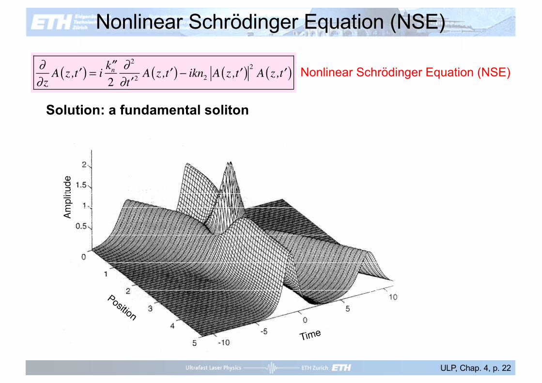
Nonlinear Schrödinger Equation (NSE)
∂∂z
A z, ′t( ) = i ′′kn2
∂ 2
∂ ′t 2A z, ′t( ) − ikn2 A z, ′t( ) 2 A z, ′t( ) Nonlinear Schrödinger Equation (NSE)
Solution: a fundamental soliton
ULP, Chap. 4, p. 24

Nonlinear Schrödinger Equation (NSE)
∂∂z
A z, ′t( ) = i ′′kn2
∂ 2
∂ ′t 2A z, ′t( ) − ikn2 A z, ′t( ) 2 A z, ′t( ) Nonlinear Schrödinger Equation (NSE)
Solution: higher order soliton (example: second order)
ULP, Chap. 4, p. 23
Soliton Period φ0 z = z0( ) = π4
⇒ z0 =π2
τ 2
′′kn

Higher-Order Soliton Pulses• Inject a pulse with N2–times the fundamental soliton energy:
periodically evolving higher-order soliton pulse (N is an integer).
• Initial condition: N = 2 for second-order soliton
• Soliton period:
becomes short for short pulses and strong dispersion
• At certain locations, significantly shorter (but not sech2-shaped) pulses occurimportant for pulse compression
• Note: soliton period is an important parameteralso for fundamental solitons:length scale on which the interaction is significant (periodic perturbation)
φ0 z = z0( ) = π4
⇒ z0 =π2
τ 2
′′kn
A 0, ′t( ) = N A0sech′tτ
⎛⎝⎜
⎞⎠⎟

Optical communication with repeaters
ULP, Chap. 4, p. 25

Optical communication with solitons
ULP, Chap. 4, p. 26

Optical communication with solitons
Δω−Δω 0
ULP, Chap. 4, p. 27

Periodic perturbation of solitons
ULP, Chap. 4, p. 27-31
∂∂z
A z, ′t( ) = i ′′kn2
∂ 2
∂ ′t 2A z, ′t( ) − ikn2 A z, ′t( ) 2 A z, ′t( ) + iξ δ z − nza( )
n=−∞
∞
∑ A z, ′t( )
NSE + periodic perturbation period za
Important for modelocked lasers:
periodic perturbation per round-trip through output coupler, gain crystal …

Periodic perturbation of solitons∂∂z
A z, ′t( ) = i ′′kn2
∂ 2
∂ ′t 2A z, ′t( ) − ikn2 A z, ′t( ) 2 A z, ′t( ) + iξ δ z − nza( )
n=−∞
∞
∑ A z, ′t( )
NSE + periodic perturbation period za
A z, ′t( ) = As z, ′t( ) + u z, ′t( )
As z, ′t( ) = A0sech′tτ
⎛⎝⎜
⎞⎠⎟ e− iφ0
u z, ′t( ) << As z, ′t( )
Assuming small perturbation: AnsatzSolution without perturbationSoliton pulse:
It can be shown that:
with the solution:
∂∂zu z, ′t( ) ≈ i ′′kn
2∂ 2
∂ ′t 2u z, ′t( ) + iξ δ z − nza( )
n=1
∞
∑ As z, ′t( )
u z,ω( ) =1za
ξA0πτsechπ2τω⎛
⎝⎜⎞⎠⎟
nka −′′kn 2
1τ 2
+ω 2⎛⎝⎜
⎞⎠⎟
ei nka−
12τ 2
′′kn ⎛⎝⎜
⎞⎠⎟
z
n=1
∞
∑Resonance effects!
ULP, Chap. 4, p. 27-31

Periodic perturbation of solitons
ULP, Chap. 4, p. 27-31
∂∂z
A z, ′t( ) = i ′′kn2
∂ 2
∂ ′t 2A z, ′t( ) − ikn2 A z, ′t( ) 2 A z, ′t( ) + iξ δ z − nza( )
n=−∞
∞
∑ A z, ′t( )
NSE + periodic perturbation period za
Periodic perturbation has no resonance effects:
In this regime periodic perturbation can be considered as a continuous perturbation.
Soliton period
… the perturbation period has to be made smaller for shorter pulses.
u z,ω( ) << As z,ω( ) ⇔ za << 8z0
z0 =π2
τ 2
′′kn ∝τ 2

Periodic perturbation of solitons
ULP, Chap. 4, p. 27-31
∂∂z
A z, ′t( ) = i ′′kn2
∂ 2
∂ ′t 2A z, ′t( ) − ikn2 A z, ′t( ) 2 A z, ′t( ) + iξ δ z − nza( )
n=−∞
∞
∑ A z, ′t( )
NSE + periodic perturbation period za
Periodic perturbation has no resonance effects:
u z,ω( ) << As z,ω( ) ⇔ za << 8z0
Dλ = 17 pskm ⋅nm

Delayed Nonlinear Response
• Intensity-dependent phase change is not always instantaneous:• Electronic contribution (usually dominating): response time
<1 fs (nearly instantaneous) in typical solids• Lattice contribution: excitation of phonons:
• Optical phonons: Raman effect(positive and negative charges oscillating in anti-phase)
• Acoustical phonons: Brillouin effect(positive and negative charges oscillating in phase)
• Beating between different optical frequency componentsexcites phonons.
• Phonons create moving index gratings which can couple light waves with different propagation directions and frequencies. Pump photon can split into Stokes photon and a phonon.

Delayed Raman ResponseOptical phonons have high frequencies (e.g. around
13 THz for silica), only weakly dependent on wave vector:
Consequence: phase matching possible forforward and backward direction:
kpks
kphonon
kp
kphononks
k
Ω optical phonons
acoustical phonons
range of interest

Raman Gain Spectrum of Silica
gain spectrum1000-nm pump
1.4
1.2
1.0
0.8
0.6
0.4
0.2
0.0
Ram
an g
ain
(a. u
.)
1120108010401000
wavelength (nm)
• Maximum gain at ≈40-50 nm wavelength offset(depends on pump wavelength)
• Gain rises ≈linearly for small offsets• Influence of composition of the fiber core (Ge, P etc.)
gR (Δω )

Intra-Pulse Raman Scattering
Principle:• Energy transfer within the pulse spectrum:⇒ center wavelength drifts
towards longer values
• Soliton interaction preserves the pulse shape
Note: Raman gain is small for small frequency offsets⇒ effect is significant only for femtosecond (soliton) pulses
shift per meter: roughly prop. to (1/τ )4
λ
J. P. Gordon, Opt. Lett. 11 (10), 662 (1986)
Examples:
• Wavelength shift from 1.56 µm to 1.78 µm:N. Nishizawa et al., IEEE Photon. Technol. Lett. 11 (3), 325 (1999)
• Wavelength shift from 1.06 µm to 1.33 µm (in holey fiber):J. H. V. Price et al., JOSA B 19 (6), 1286 (2002)

Raman Response of Silica
4
3
2
1
0
-110008006004002000
delay time τ (fs)
Damped oscillation with ≈13 THz:strong contribution, if two optical waveswith ≈13 THz frequency difference beat
R. H. Stolen et al., JOSA B 6 (6), 1159 (1989)
Response function

Generalized NSE
∂A z, ′t( )∂z
− i2
′′kn∂2A z, ′t( )
∂ ′t 2− 16
′′′kn∂3A z, ′t( )
∂ ′t 3
= −iγ A z, ′t( ) 2 A z, ′t( ) − iω0
∂∂ ′t
A z, ′t( ) 2 A z, ′t( )( ) − TRA z, ′t( ) ∂ A z, ′t( )∂ ′t
2⎡
⎣⎢⎢
⎤
⎦⎥⎥
second and third-order dispersion
SPM self-steepening RamanTR sets slope of Raman gain
γ = n2ω0
cAeff
self-frequency shift
intensity dependence of group velocity
shock formation
intensity dependence of phase velocity
Raman and self-steepening lead to asymmetry in SPM broadened spectra

Self-steepening and SPM (without GDD and Raman)
40
30
20
10
0
Pow
er [k
W]
-80 -60 -40 -20 0 20 40 60 80Time [fs]
Example: 50 fs, center wavelength 800 nm, fiber core diameter 1.7 µm and
Self-steeping means that group velocity is intensity dependent: peak moves at a lower speed than the wings
n2 = 2.5 ⋅10−20 m2 / W
Input: Gaussian pulse at z = 0
z = 3 mm (dashed) z = 6 mm
z = 6 mm (solid)
s = 1ω0τ
= T2πτ
= 0.01
16
14
12
10
8
6
4
2
0
Ener
gy/W
avel
engt
h [p
J/nm
]1.11.00.90.80.70.60.50.4
Wavelength [um]
asymmetry in SPM broadened spectrum

Self-steepening, SPM and GDD>0 (no Raman)
14
12
10
8
6
4
2
0
Pow
er [k
W]
-200 -100 0 100 200Time [fs]
16141210
86420
Ener
gy/W
avel
engt
h [p
J/nm
]
1.00.90.80.70.6Wavelength [um]
8
6
4
2
0
Pow
er [k
W]
2000-200Time [fs]
Example: 50 fs, center wavelength 800 nm, fiber core diameter 1.7 µm andGDD 3.5 fs2/100 µm
n2 = 2.5 ⋅10−20 m2 / W
s = 1ω0τ
= T2πτ
= 0.01
14
12
10
8
6
4
2
0Ener
gy/W
avel
engt
h [p
J/nm
]
1.00.90.80.70.6Wavelength [um]
z = 6 mm
z = 12 mm
40
30
20
10
0
Pow
er [k
W]
-80 -60 -40 -20 0 20 40 60 80Time [fs]
16
14
12
10
8
6
4
2
0
Ener
gy/W
avel
engt
h [p
J/nm
]
1.11.00.90.80.70.60.50.4Wavelength [um]

Saturable gain and absorber
Fläche A
Wirkungsquerschnitt σ
Dicke Δz
Dichte der Atome
EinfallendeLichtintensität
g z( ) ≡ NVσ α0 =
N0
Vσ
α = α0
1+ I Isat ,A
σ A = σ L = σg = g0
1+ I Isat ,L
Isat ,L =hνστ L
Assuming: two-level system
Isat ,A = hνστ A

Semiconductor saturable absorber
Appl. Phys. B 73, 653, 2001

Nonlinear transmission of cw beam
Assume homogeneous two-level absorption saturation:
dI z( )dz
= −2α I( ) I z( ) = − 2α0
1+I z( )Isat
I z( )
1I
1+ IIsat
⎛⎝⎜
⎞⎠⎟dI = − 2α0 dz
lnT + IinIsat
T −1( ) = −2α0d
Iin << Isat
T ≈ e−2α0d
T ≡ IoutIin Iin Isat