nonlinear response and stability analysis of vessel

NONLINEAR RESPONSE AND STABILITY ANALYSIS OF

VESSEL ROLLING MOTION IN RANDOM WAVES USING

STOCHASTIC DYNAMICAL SYSTEMS

A Dissertation

by

ZHIYONG SU

Submitted to the Office of Graduate Studies of Texas A&M University

in partial fulfillment of the requirements for the degree of

DOCTOR OF PHILOSOPHY

August 2012

Major Subject: Ocean Engineering

NONLINEAR RESPONSE AND STABILITY ANALYSIS OF

VESSEL ROLLING MOTION IN RANDOM WAVES USING

STOCHASTIC DYNAMICAL SYSTEMS

A Dissertation

by

ZHIYONG SU

Submitted to the Office of Graduate Studies of Texas A&M University

in partial fulfillment of the requirements for the degree of

DOCTOR OF PHILOSOPHY

Approved by:

Chair of Committee, Jeffrey M. Falzarano Committee members, Loren D. Lutes Richard Mercier Moo-Hyun Kim Alan Palazzolo Head of Department, John Niedzwecki

August 2012

Major Subject: Ocean Engineering

iii

ABSTRACT

Nonlinear Response and Stability Analysis of Vessel Rolling Motion in Random Waves

Using Stochastic Dynamical Systems. (August 2012)

Zhiyong Su, B.S.; M.S., Shanghai Jiao Tong University

Chair of Advisory Committee: Dr. Jeffrey M. Falzarano

Response and stability of vessel rolling motion with strongly nonlinear softening

stiffness will be studied in this dissertation using the methods of stochastic dynamical

systems. As one of the most classic stability failure modes of vessel dynamics, large

amplitude rolling motion in random beam waves has been studied in the past decades by

many different research groups. Due to the strongly nonlinear softening stiffness and the

stochastic excitation, there is still no general approach to predict the large amplitude

rolling response and capsizing phenomena. We studied the rolling problem respectively

using the shaping filter technique, stochastic averaging of the energy envelope and the

stochastic Melnikov function. The shaping filter technique introduces some additional

Gaussian filter variables to transform Gaussian white noise to colored noise in order to

satisfy the Markov properties. In addition, we developed an automatic cumulant neglect

tool to predict the response of the high dimensional dynamical system with higher order

neglect. However, if the system has any jump phenomena, the cumulant neglect method

may fail to predict the true response. The stochastic averaging of the energy envelope

iv

and the Melnikov function both have been applied to the rolling problem before, it is our

first attempt to apply both approaches to the same vessel and compare their efficiency

and capability. The inverse of the mean first passage time based on Markov theory and

rate of phase space flux based on the stochastic Melnikov function are defined as two

different, but analogous capsizing criteria. The effects of linear and nonlinear damping

and wave characteristic frequency are studied to compare these two criteria. Further

investigation of the relationship between the Markov and Melnikov based method is

needed to explain the difference and similarity between the two capsizing criteria.

v

ACKNOWLEDGMENTS

I firstly would like to express my sincere gratitude and special thanks to my advisor,

Dr. Jeffrey Falzarano. This dissertation can never been done without his support,

encouragement and guidance during my studies at Texas A&M University. I also would

like to thank Dr. Loren Lutes for his continuous communication, discussions and support

which always lead me to the right research direction. I greatly appreciate Dr. Mercier, Dr.

Kim, and Dr. Palazzolo for their review and comments for my research topics and

serving as committee members.

I am grateful to the librarians in the university library, for helping me get any

research papers, reports and books around the world using “Get it for me” service.

The work has been funded by the Office of Naval Research (ONR) T-Craft Tools

development program ONR Grant N00014-07-1-1067. I would like to thank the program

manager Kelly Cooper for her support.

Lastly, and most importantly, I would like to thank my parents and all other family

members for their continuous support and trust. Special thanks are expressed to my wife,

Yusha, for her love, optimism, sacrifices and the wonderful gift, our baby girl.

vi

TABLE OF CONTENTS

Page

ABSTRACT ..................................................................................................................... iii

ACKNOWLEDGMENTS .................................................................................................. v

TABLE OF CONTENTS .................................................................................................. vi

LIST OF FIGURES ........................................................................................................ viii

LIST OF TABLES ........................................................................................................... xii

CHAPTER

I INTRODUCTION ......................................................................................... 1

1.1 Physical Fundamentals of Vessel Dynamics ........................................... 3 1.2 Discussion of Intact Stability Failures Modes ......................................... 7 1.3 Literature Review................................................................................... 10 1.4 Methods and Procedure .......................................................................... 16

II FUNDAMENTALS OF STOCHASTIC DYNAMICS ............................... 18

2.1 Introduction to Stochastic Dynamics Systems ....................................... 18 2.2 Brownian Motion and Markov Process ................................................. 21 2.3 Stochastic Differential Equations - SDE ................................................ 24 2.4 The Derivation of Fokker Planck Equation from the SDE .................... 27

2.4.1 The derivation of the FPE from the one dimensional SDE .......... 27 2.4.2 Derivation of FPE from general SDE ........................................... 30 2.4.3 Discussion of the Fokker Planck equation .................................... 33

III THE CUMULANT NEGLECT METHOD APPLICATION TO THE NONLINEAR ROLLING RESPONSE ....................................................... 35

3.1 Modeling of Rolling Motion with Filter Application ............................ 38 3.1.1 Modeling of ship rolling ............................................................... 38 3.1.2 Modeling of rolling excitation moment ........................................ 42 3.1.3 State space formation of rolling motion........................................ 46

3.2 The Cumulant Neglect Closure Method ................................................ 48 3.2.1 Gaussian cumulant neglect method without automatic neglect tool ................................................................................................ 49

vii

3.2.2 The higher order cumulant neglect method with automatic neglect tool .................................................................................... 57

IV MARKOV AND MELNIKOV BASED APPROACHES FOR STABILITY ANALYSIS ........................................................................... 85

4.1 Introduction ............................................................................................ 86 4.2 Markov Modeling for Capsizing Analysis ............................................. 88

4.2.1 Energy based stochastic averaging ............................................... 89 4.2.1.1 Rescaling of the roll equation of motion .......................... 89 4.2.1.2 The Markov process approximation ................................. 92

4.2.2 First passage failures ................................................................... 101 4.3 The Melnikov Criterion for Capsizing Prediction ............................... 106

4.3.1 The fundamental background of the Melnikov function ............ 106 4.3.2 The rate of phase space flux ........................................................ 108

4.4 Comparison of Two Methods for Analysis of Vessel Capsizing ......... 112 4.4.1 Effects of linear and nonlinear damping coefficients ................. 113 4.4.2 The effect of characteristic wave frequency ............................... 117

V CONCLUSIONS AND FUTURE EXTENSIONS .................................... 120

5.1 Conclusions .......................................................................................... 120 5.2 Future Recommendations .................................................................... 121

REFERENCES ............................................................................................................... 124

APPENDIX A DERIVATION OF NONLINEAR COUPLED EQUATIONS OF MOTION ........................................................................................... 134

APPENDIX B DERIVATION OF DRIFT AND DIFFUSION COEFFICIENTS FOR STOCHASTIC AVERAGING .................................................. 138

VITA .............................................................................................................................. 142

3.2.2.1 Application to stochastic dynamical systems with analytical solutions....................................................................................................60

3.2.2.2 Application to rolling motion with filter......................................81 3.3 Discussions of the moment equations................................................................83

viii

LIST OF FIGURES

Fig. 1. Body fixed coordinate system x-y and principal system xN - yN ......................... 6

Fig. 2. Illustration of the SCK equation (2.8) (Moe, 1997) ........................................... 24

Fig. 3. Added mass of T-AGOS .................................................................................... 40

Fig. 4. Linear added damping coefficient...................................................................... 41

Fig. 5. Rolling moment amplitude per unit wave height ............................................... 41

Fig. 6. GZ curve of T-AGOS (C1=3.618m,C3=-2.513m) ............................................ 42

Fig. 7. Comparison of original force spectrum with filtered spectrum ......................... 46

Fig. 8. Transient response of root mean square of rolling angle ................................... 53

Fig. 9. Transient response of root mean square of rolling velocity ............................... 54

Fig. 10. Effect of nonlinear damping coefficient ............................................................ 56

Fig. 11. Effect of nonlinear stiffness coefficient ............................................................. 56

Fig. 12. Effect of linear stiffness coefficient ................................................................... 57

Fig. 13. Automatic Cumulant Neglect Tool procedure ................................................... 59

Fig. 14. Analytical probability density function of unimodal Duffing oscillator............ 61

Fig. 15. Mean square of displacement with different cumulant neglect order ................ 63

Fig. 16. Mean square of velocity with different cumulant neglect order ........................ 63

Fig. 17. Analytical probability density function of x1 x2 x3 and x4 ................................. 66

Fig. 18. Mean square of x1 with different cumulant neglect order and exact solution.... 67



ix


Fig. 22. Analytical probability density function of z ...................................................... 70

Fig. 23. Mean square of z with different cumulant neglect order and exact solution ..... 71

Fig. 24. Analytical probability density function of x and x ......................................... 73

Fig. 25. Mean square of 1x with different cumulant neglect order and exact solution .... 74


Fig. 27. Instability of cumulant neglect method with 8th order closure for mean square of 1x ........................................................................................................ 76

Fig. 28. Instability of cumulant neglect method with 8th order closure for mean square of 2x ........................................................................................................ 76

Fig. 29. Analytical probability density function of bimodal Duffing oscillator.............. 78

Fig. 30. Marginal probability density function of Duffing oscillator .............................. 78



Fig. 33. Instability of cumulant neglect method with 8th order closure ......................... 80

Fig. 34. Instability of cumulant neglect method with 8th order closure ......................... 81

Fig. 35. Evolution of the root mean square of the Rolling Displacement ....................... 82

Fig. 36. Evolution of the root mean square of the Rolling Velocity ............................... 83

Fig. 37. Phase plane for undamped and unforced oscillator ........................................... 94

Fig. 38. Fourier expansion of0sin Φ and

0cosΦ at 0E =0.01 and n=1 ............................. 97


0cosΦ at 0E =0.2499 and n=1...3 .................... 97


0cosΦ at 0E =0.2499 and n=1...5 .................... 98

x

Fig. 41. Drift coefficients for varioussH , Unit: Meter ................................................... 98

Fig. 42. Diffusion coefficients for varioussH , Unit: Meter ............................................ 99

Fig. 43. Drift coefficients for variouszω ,

sH =5m ......................................................... 99

Fig. 44. Diffusion coefficients for variouszω ,

sH =5m ................................................ 100

Fig. 45. Drift coefficients for various linear damping coefficients 1b ,

sH =5m, 2 / 9zω π= ..................................................................................................... 100

Fig. 46. Drift coefficients for various nonlinear damping coefficients 2b ,

sH =5m, 2 / 9zω π= ..................................................................................................... 101

Fig. 47. Mean first passage time with initial condition 0E , 3sH m= ........................ 104

Fig. 48. Logarithm of mean first passage time 1log 10( 0 )M（） ...................................... 105

Fig. 49. Mean first passage rate 11/M 0（） .................................................................... 105

Fig. 50. Melnikov function for 1sH m= ..................................................................... 110

Fig. 51. Melnikov function for 3sH m= .................................................................... 111

Fig. 52. Melnikov function for 5sH m= .................................................................... 111

Fig. 53. Mean first passage rate for various linear damping coefficients and sH ........ 114

Fig. 54. Normalized phase transport rate for various linear damping coefficients and

sH ............................................................................................................. 115

Fig. 55. Relation between normalized phase transport rate and mean first passage rate with different linear damping coefficients ................................................ 115

Fig. 56. Mean first passage rate for various nonlinear damping coefficients and sH .. 116

Fig. 57. Normalized phase transport rate for various nonlinear damping coefficients and

sH ............................................................................................................. 116

xi

Fig. 58. Relation between normalized phase transport rate and mean first passage rate with different nonlinear damping coefficients .......................................... 117

Fig. 59. Mean first passage rate for various characteristic wave frequency and sH .... 118

Fig. 60. Normalized phase transport rate for various characteristic wave frequency and sH ............................................................................................................. 119

Fig. 61. Variance of 0( )M τ of unit significant wave height .......................................... 119

xii

LIST OF TABLES

Table 1. ‘T-AGOS’ dimensional parameters .................................................................. 40

Table 2. Comparison of stationary mean square displacement of the unimodal Duffing oscillator ............................................................................................. 64

Table 3. Comparison of stationary mean square of state variables with different closure level and exact stationary value ........................................................... 69

Table 4. Comparison of stationary mean square of z with different closure level and exact stationary value ................................................................................ 72

Table 5. Comparison of stationary mean square of 1x and 2x with different closure level and exact stationary value........................................................................ 75

Table 6. Comparison of stationary mean square of 1x and 2x with different closure level and exact stationary value for bimodal Duffing oscillator ...................... 80

1

CHAPTER I

INTRODUCTION

Static and Dynamic stability is one the most important safety features when

designing floating offshore structures, especially for ship shaped structures. Insufficient

stability could lead to large amplitude rolling motion or even capsizing. GM based static

stability criterion were first developed back to nineteen century (Moseley, 1850), and

this approach was further refined by Rahola in 1939 (Rahola, 1939). The first

international intact stability resolutions IMO A.167 were approved by IMO in 1968 for

ships less than 100m; this criterion was mostly based on Rahola’s work (Rahola, 1939).

The IMO intact stability (IS) code has been revised several times through the 1960s to

now, but all of these codes are still based on the righting arm curve (GZ curve) in the

calm water. The reason why dynamic stability has not been applied in the IS code is the

difficulty of the nonlinear large amplitude rolling motion with the stochastic and

probabilistic approach has not been applied completely and satisfactory. The numerical

simulation in the time domain and model testing provides possible alternative ways to

approach this complex stochastic failure event. However, both methods are not easy to

apply and also require significant time and cost. Both numerical simulation and model

testing are excellent for estimating structure response, but not for stability or long term

__________________________

This dissertation follows the style and format of Ocean Engineering.

2

failure prediction. As the vessel capsizing failure is such a very rare event, analytical

methods are still the most needed technique, which provides quick and accurate

estimation of the system stability or failure. At present, International Maritime

Organization (IMO) is working on the new regulations of intact stability based on the

stochastic and probabilistic approach with dynamic effect. The sub-committee on

Stability, Load Lines and on Fishing Vessels (SLF) of IMO is discussing the next

generation of stability criterion during recent SLF meetings (SLF50/4, 2006; SLF51/4,

2008; SLF52/3, 2009) and proposed four main intact stability failure modes.

• Dead Ship Condition, i.e. ship without speed, exposed to environment

• Pure-loss of Stability

• Parametric Roll

• Surf-riding and Broaching to

Physical phenomena of the above failure modes are complex nonlinear dynamics.

For research convenience and simplicity, all of the above dynamical motions are

modeled as a single degree freedom system after decoupling from the other modes with

some appropriate assumptions. Before studying vessel stability, it is necessary to

explain the definition of an intact stability failure first. Basically, there are two types of

intact stability failure as per the SLF documents, 1) Total Intact Stability failure - total

loss of the vessel, which may be additionally combined with the loss of the lives. 2)

Partial intact stability failure - the partial loss of the vessel’s operational capabilities

combined with the additional potential danger for people as well as for cargo and

equipment. Capsizing is defined as the total intact stability failure and the capsizing is a

3

very rare event. Most capsizing accidents are related to the large angle rolling that leads

to green water on deck or equipment shift. Large angle rolling is defined as the partial

intact stability failure, which will not lead to capsizing. Only Dead Ship Condition with

random beam waves will be considered in this dissertation.

1.1 Physical Fundamentals of Vessel Dynamics

The equations of motion describing a floating rigid body are nonlinear and coupled.

The six degree of freedom equations of motion have been derived in variety of

references (Abkowitz, 1969; Falzarano, 1990; Lewandowski, 2004). These Euler’s

equations of motions are as follows, derivations can be found in the Appendix A:

2 2[ ( ) ( )]G GX m u qw rv x q r z pr q= + − − + + + (1.1)

[ ( ) ( )]G GY m v ru pw x pq r z qr p= + − + + + − (1.2)

2 2[ ( ) ( )]G GZ m w pv qu x rp q z p q= + − + − − + (1.3)

44 55 66 64( ) ( )

( )G

K I p I I qr I r pq

mz v ru pw

= − − − +− + −

(1.4)

2 255 66 44 64( ) ( )

( ) ( )G G

M I q I I rp I r p

mz u qw rv mx w pv qu

= − − − −+ + − − + −

(1.5)

66 44 55 64( ) ( )

( )G

N I r I I pq I p qr

mx v ru pw

= − − − −− + −

(1.6)

where m is the mass of the ship, 44I ,

55I ,66I and

64I are the moments and cross products

of inertia in the body fixed system, which always put its origin at the mid-ship and

design waterline, the subscripts represent respectively: 4=roll, 5=pitch, 6=yaw. u, v, w

4

are the velocity of the translational motions, surge, sway and heave; p q r are the angular

velocity of the rotational motions, roll, pitch and yaw. Gx and

Gz are the coordinates of

ship center of gravity in the body fixed system. X ,Y ,Z ,K ,M ,N are applied force

and moments in the body fixed system, representing the hydrodynamic and hydrostatic

forces and moments. The total hydrodynamic and static forces are assumed as the

summation of various components: including Froude-Krylov forces, diffraction forces,

and radiation forces, viscous nonlinear damping force and hydrostatic restoring force.

These coupled nonlinear equations are difficult if not impossible to get analytical

solution to, so approximation and assumption must be made for any real progress.

Considering small motions, the Euler’s equations of motions of equations (1.1) to (1.6)

could be linearized to drop the nonlinear inertial terms. Following the derivations of

Vugts (Vugts, 1970), the linearized equations of motions are as follows:

[ ]GX m u z q= + (1.7)

[ ]G GY m v x r z p= + − (1.8)

[ ]GZ m w x q= − (1.9)

44 64 GK I p I r mz v= − − (1.10)

44 ( )G GM I q m z u x w= + − (1.11)

66 64 GN I r I p mx v= − + (1.12)

Due to the port and starboard symmetry, the linearized equations have no inertial

coupling terms between longitudinal (surge, heave and pitch) and lateral (sway, roll and

yaw) modes. In order to better understand the complicated nonlinear dynamics of vessel

5

rolling motion, it is necessary to decouple the rolling mode from the other six degrees of

freedom linearized equations.

In this dissertation, we consider beam waves only, so the yaw mode motion is

small and negligible when considering the ship is fore-aft symmetric approximately, and

therefore only the coupling between the sway and roll is considered. The linear two

degree of freedom equations describing roll and sway:

44

G

G

ym mz Y

mz I Kφ

⎡ ⎤⎡ ⎤ ⎡ ⎤− ⎢ ⎥⎢ ⎥ ⎢ ⎥=⎢ ⎥⎢ ⎥ ⎢ ⎥−⎢ ⎥ ⎢ ⎥⎢ ⎥⎣ ⎦ ⎣ ⎦⎣ ⎦ (1.13)

where y is the sway displacement and φ is the roll angle; y v= and pφ = ; Note that

the mass and moment inertial term m and 44I could also include the virtual mass and

inertial. It is possible to find a new coordinate system that could remove the coupling

term in the above equation. The two equations can be solved independently after the

decoupling. The new coordinates are called principal coordinates or normal coordinates.

Let us assume the distance between the new coordinate system xN - yN and the original

system x - y is cR . From the rigid body dynamics displayed in the Fig. 1, the relation

involving the acceleration of the points on the body are given by below,

N c N

N

y y R φφ φ

⎧ = +⎪⎪⎨⎪ =⎪⎩ (1.14)

We also need to replace the forces and moments with equivalent force and moment in

the new coordinate system,

6

N

N c

Y Y

K K mRY

⎧ =⎪⎪⎨⎪ = −⎪⎩ (1.15)

By substituting the equations (1.14) and (1.15) back into (1.13), we get the decoupled

equations with c GR z= ,

44

0

0N N

N NN

ym Y

I Kφ

⎡ ⎤⎡ ⎤ ⎡ ⎤⎢ ⎥⎢ ⎥ ⎢ ⎥=⎢ ⎥⎢ ⎥ ⎢ ⎥⎢ ⎥ ⎢ ⎥⎢ ⎥⎣ ⎦ ⎣ ⎦⎣ ⎦

(1.16)

where 244 44N GI I mz= − ;

Fig. 1. Body fixed coordinate system x-y and principal system xN - yN

The decoupled single degree freedom roll equation (Lewis et al., 1989) is

considered in this dissertation for response and stability analysis,

7

3

44 44 44 44 1 3( ( )) ( ) ( ) ( ..) ( )N qI A B B C C f tω φ ω φ ω φ φ φ φ+ + + +Δ + + = (1.17)

Linear added mass 44( )A ω and added damping 44( )B ω coefficients are from linear

potential theory, which can be calculated by many hydrodynamic program, e.g., Strip

Theory based SHIPMO (Beck and Troesch, 1990), or Three-Dimensional panel based

WAMIT (Lee and Newman, 2009), AQWA (ANSYS, 2010), and MOSES (Ultramarine,

2010). We will use 44I to replace the notation 44NI in this dissertation for convenience.

The constant Δ is the displacement of the vessel and 1C , 3C are the linear and cubic

nonlinear stiffness coefficients. 44qB is the quadratic viscous damping coefficients for

roll motion, which is determined on a component basis (Falzarano, 1990) and is

redefined and incorporated into SHIPMO. f is the external moment from wave

excitation. The moment term in this dissertation is limited to linear excitation due to the

limitation of available hydrodynamic code SHIPMO. However, the nonlinear part of the

hydrodynamic force could also be considered for the large amplitude rolling motion

(Kim, 2008). The damping moment, stiffness moment and external moment are part of

NK in equation (1.16). How to calculate the hydrodynamic forces and how to analyze the

rigid body dynamics are the two major problems when studying the rolling motions.

1.2 Discussion of Intact Stability Failures Modes

The simplified and decoupled equation (1.17) is the generalized rolling math model.

Based on the simple rolling model, the math modes for failure modes are described

differently.

8

According to (Belenky et al., 2008), Pure-loss of stability and Parametric Roll both

related to the variation of the restoring moment in waves. The restoring moment

becomes larger in the wave trough and smaller on the wave crest due to the variation of

hull geometry underwater. When the ship is sailing in the following or head seas and the

wave length is comparable to the ship length, the variation of GZ is most evident. Pure

loss of stability in waves means when the vessel spends enough time on the wave crest

in the following or quartering waves, the stability becomes smaller and less than the

heeling moments and then the vessel may experience capsize or large amplitude angle

motion. Parametric roll or parametric roll resonance is a result of periodic changes of

stability at some frequency related to the natural frequency of the rolling motion. The

major approach researching parametric rolling is Mathieu equation and related Ince-

Strutt diagram, which is a common approach in nonlinear dynamics to predict the stable

and unstable zone for given parameters. Broaching to is also defined as a mode of intact

stability failure, which is related to the maneuvering problem: surf-riding. Instead of

researching the decoupled rolling equation for parametric rolling, the nonlinear math

model for broaching is surge mode equation with resistance force and propeller force.

The most classic stability failure mode is considering the beam waves with

constant restoring moment, the so called “Dead Ship Condition”. When a ship engine

loses power during operation, the environment will turn the ship to the beam seas

condition. How to analyze the vessel rolling dynamics in the beam waves is the main

purpose of this dissertation. When considering regular beam wave excitation and

neglecting the wind excitation, equation (1.17) with constant added mass, damping and

9

stiffness coefficients is a widely accepted mathematical model for large amplitude

rolling motion or capsizing research. However, it has to be noted that the wave force is a

stochastic or random process, which means the wave excitation cannot be modeled as a

regular input and the time invariant system is questionable. For a single harmonic

excitation, added mass and linear damping takes values at the input wave frequency. For

excitation with narrow banded excitation, the values may be evaluated at the peak

frequency of the input excitation. For wide band excitation, the values at the natural

frequency may be a better approximation (Jiang et al., 2000).

Alternatively, the time domain model can overcome the variation of hydrodynamic

coefficients in the frequency domain. Following (Ogilvie, 1964), the time domain ship

rolling model that describes the realistic response in random waves is given as following

with convolution integral:

44 44 03

44 1 3

( ( )) ( ) ( )

( ..) ( )

t

q

I A K t d

B C C f t

φ τ φ τ τ

φ φ φ φ

+ ∞ + −

+ +Δ + + =∫ (1.18)

where 44( )A ∞ is the added mass coefficient at infinite frequency, ( )K t τ− is the

retardation function or impulse response function (IRF) of velocity, which is determined

by the geometry of the ship hull. The IRF and the frequency domain hydrodynamic

coefficients are related by cosine or sine transform, see e.g. (Cummins, 1962; Ogilvie,

1964). The quadratic damping term44qB is usually treated as approximately constant and

independent of frequency.

The time domain equation (1.18) gives a more accurate representation of the dead

ship condition stability model compared with the constant coefficients model equation

10

(1.17) for the study of rolling stability in random beam waves. However, the convolution

integral also introduces additional difficulties when using traditional methods of

stochastic dynamical system. The final goal of the rolling stability in the dead ship

condition is to analytically calculate the response and the capsizing probability based on

the decoupled time domain math model. As an initial stage research, we will first focus

on the constant coefficients model.

1.3 Literature Review

Research on motions or dynamics of ships and offshore structures in random seas has

been studied over the century. It is important to study the highly nonlinear large

amplitude rolling motion of ship shaped structures, due to the its strong effect on the

stability and safety, or even capsizing. Basically, there are two major obstacles to

completely understand the highly nonlinear dynamics of offshore structures:

hydrodynamic force computation and rigid body dynamics. The coefficients for the

equations of rigid body dynamics and force excitation are determined from the

hydrodynamics computations. Most current time domain commercial software for

motion predications are based on numerical simulation of dynamical system after first

determining the hydrodynamics coefficients. When considering the nonlinear effects on

motions, e.g. nonlinear damping, nonlinear restoring force, or nonlinear excitation, etc;

people have to be cautious when applying the direct numerical simulation, especially

when the nonlinear effect is strong. Analytical methods are still the most needed

11

technique for understanding the nonlinear behavior of vessel motions, like the typical

vessel rolling analysis.

Mathematical research models for vessel dynamics include both coupled multi

degrees of freedom (Falzarano and Zhang, 1993; Zhang and Falzarano, 1994; Spyrou,

1996a; Spyrou, 1996b; Spyrou, 1997; Ibrahim and Grace, 2010) and also decoupled

single degree freedom of system, especially rolling motion (Roberts, 1982; Roberts,

1982; Roberts and Spanos, 1986; Falzarano, 1990; Falzarano et al., 1992; Lin and Yim,

1995; Roberts and Vasta, 2000; Francescutto and Naito, 2004; Jamnongpipatkul et al.,

2011; Su and Falzarano, 2011). Rolling motion is nonlinear and coupled with the other

modes of motions: sway, yaw and pitch, etc. It is reasonable to model the rolling motion

as a single degree of freedom equation (SDOF) in two special cases: one is the ship

rolling in unidirectional head or following seas, which will lead to parametric rolling

analysis using popular Mathieu chart or Hill chart. The other one is the ship rolling in

unidirectional beam seas at low or zero speed, provided that we consider the coordinate

origin to be located at a pseudo ‘roll center’ (Roberts and Vasta, 2000).

Analytical studies of rolling motion under beam sea were first initiated by Froude

(Froude, 1861), he derived the SDOF rolling equation including nonlinear damping and

restoring moment terms. Nonlinear terms in the roll equation may lead to very

complicated behavior of the ship rolling response. Stability is the most important issue

for naval architects and ocean engineers. Traditionally, the only static intact stability is

considered for practical design purpose. More and more researchers have found that

hydrodynamic induced damping, wave exciting force, initial conditions and green water

12

on deck are also important to ship stability. Due to the nonlinearity of the damping and

stiffness, we are unable to find the analytical solution for even the single degree freedom

system of the general second order ordinary differential equation, even when the

excitation force is only harmonic.

The response of nonlinear rolling motion in regular waves is a nonlinear dynamics

problem with harmonic excitation, which may generate super harmonic, sub harmonic

(Cardo, 1981; Cardo et al., 1984),or even chaos phenomena (Thompson, 1990;

Thompson, 1992). Cardo and Francescutto applied harmonic excitation to the SDOF

rolling motion and investigated three different mechanisms for the onset of super and

sub harmonics phenomenon. Thompson (Thompson, 1990) proposed the conception of

safe basin and basin erosion with harmonic direct and parametric excitation and

introduced that the transient motions induced capsize should be paid more attention than

steady state conditions. Different initial conditions under harmonic excitation will be

attracted to different steady state oscillations or divergent solutions. The safe basin is

defined as the area of initial conditions which are attracted to the bounded steady state

solutions. With the increasing direct or parametric excitation, the erosion of safe basin

will reduce the safe area significantly. Also the frequency of excitation close to the

natural frequency of rolling is found to be the worst excitation scenario. Virgin (Virgin,

1987) studied the chaotic rolling motions in regular beam waves for SDOF rolling model

using a semi empirical roll model. Qualitative prediction techniques for the possibility

of capsizing were utilized using dynamical system theory. Nayfeh (Nayfeh, 1986a;

13

Nayfeh, 1986b; Nayfeh, 1990) applied Floquet and bifurcation theory to study the local

stability of the dynamical system with steady state solutions.

It is more accurate to consider the randomness of the excitation force than just

considering harmonic force for vessel motions in realistic waves. How to understand the

possibility of capsizing of ships in realistic waves is a very challenging research topic

even only considering the SDOF rolling model. The math model for the SDOF rolling

model with random forces is a nonlinear random vibration problem. Many different

research groups have made contributions to analyzing the rolling stability in the sense of

random waves. Roberts (Roberts, 1982; Roberts, 1982; Roberts and Spanos, 1986;

Roberts et al., 1994; Roberts and Vasta, 2000) have studied the rolling problem for more

than two decades using stochastic averaging technique. By modeling the energy

envelope of system response as a continuous Markov process, the one dimensional

energy process satisfies the Fokker Planck Equation, which will be introduced in the

next chapter. The drift and diffusion coefficients could be evaluated by the two state

variable rolling equation’s system parameters. The issue of the stochastic averaging of

the energy envelope is limited to the light damping. However, the statistics of first

passage time to approach the critical boundary can be evaluated from the one

dimensional Markov process and the associated Fokker Planck Equation.

Since the rolling response satisfies the Fokker Planck Equation, which is a partial

differential equation (PDE), many researchers also have contributed to numerically

solving the PDE. The path integral method is the most popular numerical tool for the

analysis of random rolling response. The research group of Yim (Lin and Yim, 1995;

14

Yim et al., 2005) first applied the path integral method to a harmonic plus white noise

excited rolling system and then to a filtered white noise excited roll-heave coupled

system. The application of the path integral method to the stochastic rolling process can

be also found from different authors (Liqin and Yougang, 2007; Cottone et al., 2009;

Jamnongpipatkul et al., 2011). Instead of the numerical solution, Francescutto

(Francescutto and Naito, 2004) utilized moment equations to study a six dimensional

stochastic system with four Gaussian filter variables using the Gaussian cumulant

neglect method. The author investigated the effect of linear and nonlinear damping, and

righting moment effect on the statistics of the rolling response. There is no limitation on

the damping and force magnitudes for both moment equations and path integral methods.

The difficulty for the filtered system is the high dimension, which is always to be

avoided by researchers when dealing with stochastic systems.

Geometric methods have been applied to many nonlinear systems, especially to the

nonlinear ship rolling model. Instead of directly studying the stochastic differential

equation, the geometric methods try to analyze the problem in the sense of phase space

for qualitative behavior. The Melnikov method was initially introduced into Naval

Architecture by Falzarano (Falzarano, 1990; Falzarano et al., 1992) for harmonic

excitations. And the conception of phase space flux rate with random excitation was

applied to dynamical systems by Frey and Simiu (Frey and Simiu, 1993). Then the

Michigan research group continued to extend the Melnikov method with stochastic

excitation to large amplitude rolling motion with both constant coefficients (Hsieh et al.,

1994) and a time domain memory included model (Jiang et al., 2000). The dynamical

15

system with memory or a convolution term is a high dimensional system when extending

the convolution integral into a linear state space model (Holappa and Falzarano, 1999).

High dimensional stochastic problems are difficult and challenging question in random

vibration. Jiang successfully applied the Melnikov method to understand the stability of

stochastic system without extending the convolution term to extended state space model.

Considering periodic excitation with random white noise disturbance, Lin and Yim (Lin

and Yim, 1995) developed a generalized Melnikov method to predict upper bound of

potential chaotic roll motion and further capsizing possibility. Chen and Shaw (Chen,

1999) introduced a systematic approach to modeling multi degree freedom ship motions

with regular excitation input. Bikdash (Bikdash et al., 1994) studied different damping

models for rolling dynamics and derived a condition that linear-plus-cubic and linear-

plus-quadratic model yields the same Melnikov predictions. Huang (Huang, 2003;

Huang, 2004) presented the safe basin erosion in random waves with energy based

Melnikov methods. He also considered the stochastic averaging method developed by

Robert to relate the capsizing phenomena and Melnikov function. Wu (Wu and McCue,

2008) used the extended Melnikov method to two rolling model in regular seas without

the constraint of small damping.

As the analytical methods for large amplitude rolling motion and capsizing analysis

have to resort to many assumptions, e.g., decoupling, low damping, low excitation,

constant hydrodynamics coefficients, etc, one of the possible solutions might be

developing numerical simulation tool considering all nonlinear hydrodynamic effect.

Belenky (Belenky and Sevastianov, 2007; Belenky et al., 2011) combining the analytical

16

method and Large Amplitude Motion Program (LAMP) to evaluate the probability of the

rare event capsizing.

1.4 Methods and Procedure

When the vessel is excited by random beam waves, the response and capsizing

problem are governed approximately by the single DOF dynamical system, equation

(1.17). The most direct method to study the response and the stability of the rolling

motion is the numerical simulation, or so called Monte Carlo simulation. As capsizing is

such a rare event, the numerical simulation provides no improvement for the practical

vessel design. Analytical methods are still the most needed technique for vessel rolling

analysis. We will study three different methods to understand the rolling response and

stability problems separately by,

• Increasing the dimension—Shaping filter technique

• Decreasing the dimension—Stochastic averaging of energy envelope

• Maintain the dimension—Melnikov Method

The fundamentals of stochastic dynamics are introduced in the Chapter II, with a

focus on Brownian motion, Markov processes, stochastic differential equations, and the

Fokker Planck Equation.

In Chapter III, the random excitation force is reproduced by using a linear filter, i.e.,

the so called shaping filter technique. This method introduces some additional Gaussian

filter variables to transform the Gaussian white noise to colored noise in order to apply

17

the Markov properties. There is no limitation on the damping or excitation magnitude for

the shaping filter technique. We will introduce the automatic cumulant neglect tool to

analyze the statistical response of the high dimensional rolling model and also discuss

the limitation of the cumulant neglect application to non Gaussian response.

In Chapter IV, the stochastic averaging of the energy of envelope decreases the two

dimension rolling system to a one dimensional energy process, which satisfies the

Markov process property under the small damping and excitation assumptions.

Compared with the Markov method, the Melnikov method analyzes the rolling capsizing

problem from the view of the phase space flux. This dissertation initially compares the

efficiency, capacity and difference of the three methods and discusses their advantages

and disadvantages respectively.

The work is summarized and future research directions are presented in Chapter V.

Finally the derivation of nonlinear coupled equation of motion and stochastic averaging

of energy envelope is given in the Appendix.

18

CHAPTER II

FUNDAMENTALS OF STOCHASTIC DYNAMICS

Probabilistic or stochastic domain methods, which are different from the traditional

frequency domain and time domain method in the offshore industry, are getting more

and more attentions in the modern analysis of dynamical system, especially when

designing new concept structures with nonlinear aspects. The loading of marine

structures due to wind and wave, are always stochastic in nature. Therefore the

probabilistic or stochastic methods are important to accurately estimate the response. A

major concern in stability problems is estimating the extreme values and the upcrossing

rate, while the probability density function (PDF) of the response signal can give the

superior results, if the response PDF is known accurately. The demand for precise

estimation of the response has motivated research on nonlinear stochastic dynamical

systems. In order to understand the whole probabilistic domain method, application for

the analysis of the stochastic dynamical systems, we first introduce the fundamentals of

stochastic dynamics.

2.1 Introduction to Stochastic Dynamics Systems

Stochastic dynamical systems or random dynamical systems are a theoretical

formulation of a dynamical system with some elements of randomness or uncertainty. It

consists of noise excitation and state variables. Analysis of stochastic dynamical systems

19

is a challenging field which has attracted many researchers for more than a century. The

theory of stochastic dynamics in general began in the nineteenth century (Fuller, 1969),

when physicists were trying to show that the heat in a medium is essentially a random

motion of the molecules. Robert Maxwell (Maxwell, 1860; Maxwell, 1867) developed

the steady state probability density function for the individual molecules. Later Ludwig

Boltzmann (Boltzmann, 1868) generalized Maxwell’s result to include the conservative

force field. The probability density function given as an exponential function of total

energy, which is known as Maxwell-Boltzmann distribution. They laid the foundation of

stochastic dynamics, even the systems they considered were conservative and

autonomous, and only initial conditions were random. Around the end of nineteenth

century, Rayleigh (Rayleigh, 1880) was the first to treat a random walk in physics and

obtained a partial differential equation for the probability density function of the

displacement. Moreover, he applied a similar technique to the theory of gas and arrived

at a PDE governing probability density function of the velocity of the gas molecules

(Rayleigh, 1891). The PDE is the first example of what was later defined as the Fokker

Planck Equation. Bachelier (Bachelier, 1900) obtained a simple Fokker Planck Equation

describing the French stock exchange. Later (1910, 1912) he studied the gambler’s ruin

which led to a moderately general Fokker Planck equation. The work developed by

Rayleigh and Bachelier have been largely unnoticed (Fuller, 1969).

In 1905, Albert Einstein (Einstein, 1905) brought the Maxwell-Boltzman theory

and the random walk method together in a paper on Brownian motion. The definition of

Brownian motion will be defined in the next section. Langevin interpreted the random

20

disturbances as an additional forcing function, which is the initiation of the stochastic

differential equations (SDE). Fokker (Fokker, 1913; Fokker, 1914) treated a first order

system with state dependent white noise. Planck (Planck, 1917) studied a n-th order

system with state dependent white noise and also generalized Fokker’s equation. And

Kolmogorov (Kolmogoroff, 1931) made the Fokker Planck Equation more general and

abstract. He also assumed the process to be a Markov process. FPE is also called Fokker

Planck Kolmogorov (FPK) or Kolmogorov’s second equation to honor his contribution.

Additionally, he also named Kolmogorov’s first equation, also known as backward

Kolmogorov equation, which is adjoint of the second equation. In 1933, Kolmogorov

(Kolmogorov, 1933) extended the theory to the vector process and also discussed the

uniqueness of the solution of the FPE.

Other early useful references to understanding the progress and history of stochastic

dynamics and the Fokker Planck Equation can be found in (Uhlenbeck and Ornstein,

1930; Wang and Uhlenbeck, 1945), (Caughey and Dienes, 1961; Caughey, 1963a)and

(Crandall and Mark, 1963). Recent developments in the analysis of stochastic dynamics,

are mostly based on the early development of Brownian motion. Analysis method for

FPE and stochastic differential equations, include statistical linearization (Caughey,

1963b; Roberts and Spanos, 1990), statistical nonlinearization (Lutes, 1970), stochastic

averaging (Roberts and Spanos, 1986; Zhu, 1988), moments closure, exponential

polynomial closure method (Er, 1998), etc. More conclusive work can be found in

classic textbooks (Soong and Grigoriu, 1993; To, 2000; Lutes and Sarkani, 2004;

Ibrahim, 2007). Stochastic differential equations and FPE have been applied to many

21

engineering and science fields, such as particle physics, structural dynamics,

aerodynamics, hydrodynamics, stock market, etc.

2.2 Brownian Motion and Markov Process

Brownian motion is named after an English botanist Robert Brown to describe the

random drift of particles in a fluid or the mathematical model used to describe such

random motions. In mathematics, Brownian motion tB , also called Wiener Process in

honor of Norbert Wiener, is characterized by following properties for the unit process;

• 0 0B =

• tB has independent increments with dB = ~ (0, ( ))t sB B N t sσ− − for

0 s t≤ ≤

• E(Bt) = 0, and E(Bt, Bs)= σ2min(t, s)

N (μ, σ2) denotes the Gaussian distribution with mean value μ and variance σ2. E

represents the expectation operation. The process is continuous everywhere but

differential nowhere. Gaussian white noise Wt is defined as the increment of the Wiener

process. From the property of the Wiener process, the increments are independent and

Gaussian distributed. So variables Wt are uncorrelated for each time t. Hence the

spectrum will be a flat curve, which means Gaussian ‘white’ noise. The mathematical

relationship is given by:

( )t tdX W dt W t dt= = (2.1)

22

( )W t is Gaussian white noise, when numerically integrated the above equation, the

response tX is the Wiener process. Therefore we related the white noise and Wiener

process by,

t tdB W dt= (2.2)

Given a stationary Gaussian white noise with power spectrum density (PSD)0s ,

0( )WWS sω = . The autocorrelation is given by,

0( ) 2 ( )WWR sτ π δ τ= (2.3)

where ( ) ( ( ) ( ))WWR E W t W tτ τ= + is the correlation function. Also notice that 0s is the

value for two side spectrum density. If we consider the one sided PSD, then

0( ) 2WWS sω = . The relation of autocorrelation and spectral density function can be

given by following Fourier transforms pairs,

1( ) ( )

2i

XX XXS R e dωτω τ τπ

+∞

−

−∞

= ∫ (2.4)

and

( ) ( ) iXX XXR S e dωττ ω ω+∞

−∞

= ∫ (2.5)

The constant spectral density of white noise implies that the energy of the random

process in uniformly distributed over whole frequency range and the autocorrelation

function with Dirac delta function means that the Gaussian white noise has infinite

variance. Such a process with infinite variance does not exist in reality, but it is a good

23

approximation to model wide band noise with very short correlation time, which is

defined as,

0

( )

(0)XX

cXX

Rd

R

ττ τ

∞

= ∫ (2.6)

where ( ) ( ( ) ( ))XXR E X t X tτ τ= + . In the study of stochastic differential equations and

stochastic systems, Gaussian white noise is a most important concept. The response of

any linear or nonlinear system driven by white noise constitutes a Markov Process and

therefore the system can be analyzed by using Markov methods.

The Markov process, named after the Russian mathematician Andrey Markov, is a

stochastic process with the Markov property, and very limited memory, namely the

process has only one step memory given below mathematically,

1 2 0 1

( , ,......, ) ( )n n n n nt t t t t tp x x x x p x x

− − −= (2.7)

where 1 2 0...n n nt t t t− −> > > and ( )p • • designates the conditional probability density

function (PDF) and ntx represent the state value at time step

nt . The above equation

means that the future state ntx depends only on current state

1ntx

−and does not depend on

any other past state values.

The well known Smoluchowski-Chapman-Kolmogorov (SCK) equation, which is

very useful when understanding the derivation of FPE, can be derived based on

equation(2.7),

1 1

( ) ( ). ( )n n n nt t t t t t tp x x p x x p x x dx

− −

+∞

−∞

= ∫ (2.8)

wh

giv

pro

Fig

2.3

mo

sto

ass

here nt t> >

ven that the

obability of

g. 2 helps to

3 Stochastic

A stochast

otion or resp

ochastic proc

sumption, th

1nt −> . The p

process sta

arriving ther

interpret the

Fig. 2. Illu

Differentia

tic differenti

ponse of th

cess, e.g. wh

e random te

probability o

arted at the

re by passin

e SCK equat

ustration of t

al Equations

ial equation

e dynamica

hite noise or

erm in the SD

of the rando

value of x

ng through a

tion.

the SCK equ

s - SDE

is an ordina

l structures

other type o

DE has to be

m variable x

1ntx

−at time t

all the possib

uation (2.8) (

ary different

with one o

of noise. To

e white nois

x arriving at

1nt − , is the

ble intermed

(Moe, 1997)

tial equation

or more of

apply the M

se. In case of

t ntx at time

summation

diate values

)

n governing

the terms is

Markov proc

f colored no

24

nt ,

of

tx .

the

s a

ess

oise

25

excitation, the limitation of white noise term can be eliminated by using a shaping filter

technique to be introduced in the next chapter. Generally, the stochastic differential

equation can be expressed with a stochastic white noise term ( )W t as below,

( , ) ( , ) ( )dtdX

F X t G X tW t= + (2.9)

where X is the vector of stochastic process, ( , )F X t is defined as drift coefficient vector,

and ( , )G X t is the diffusion coefficient matrix of the dynamical system. F and G both

have deterministic function forms with nonlinear terms if the related dynamical system

is nonlinear. The SDE above is equivalent to the general integration:

0

0 0

( , ) ( , )t t

t t

t t

X X F X d G X dBτ τ τ= + +∫ ∫ (2.10)

where0t is the initial time and

0tX represent initial condition of the stochastic process.

The first integral at RHS of the equation is an ordinary mean square Riemann-Stieltjes

integral, but the second integral is not. Here we discuss the one dimensional problem

only, however, all these results can be generalized to higher dimensions. The Riemann-

Stieltjes integration of tX with respect to a variable

tR is given by

2

1

1

1

1

( )i i i

t m

t tit

X dR X R Rτ τ τ+

−

=

≈ −∑∫ (2.11)

where 1i i iτ τ τ +≤ ≤ and

1 1 2 2.... Mt tτ τ τ= < < < = , when m → +∞ , the right

hand side will converge to the unique integral. For the second integration of (2.10)

including the Wiener processdB , the limit of the Rimann-Stieltjes integration depends

26

on evaluation point of iτ is chosen. Basically, there are two different commonly used

integral evaluation methods, namely the Itô integral, ifiτ=

iτ, and the Stratonovich

integral, if iτ= (

1i iτ τ+ + )/2.

The Itô, equation (2.12), and Stratonovich, equation (2.13) integral of the second

term of equation (2.10) are written by,

2

1

1

1

1

( )( )i i

t m

t t iit

G dB G B Bτ ττ+

−

=

≈ −∑∫ (2.12)

2

1

1

11

1

( )( )2 i i

t mi i

t tit

G dB G B Bτ τ

τ τ+

−+

=

+≈ −∑∫ (2.13)

The Stratonovich integral satisfies all the formal rules of classical calculus and therefore

it is a better choice for SDE. However, the Itô integrals are martingales and have more

advantages for computational purposes (To, 2000). The Stratonovich integral SDE

becomes equivalent to the Itô SDE by adding a modified drift term,

1)

2(

GG dtX

dX F GdB∂∂

= + + (2.14)

in which G is a matrix, the differentiation term in the parentheses is not appropriate.

Thus, above SDE can be written more explicitly,

1 1 1

1) , 1,2,3,4....

2(

n n nij

i i kj ij jj k jk

GG dt i

xdx F G dB

= = =

∂=

∂= + +∑∑ ∑ (2.15)

So the methodology for solving an Itô SDE is adapted for solving a Stratonovich SDE.

The correction term 12

GGX

∂∂

is well known as Wong-Zakai or Stratonovich correction

27

term. Note that the Itô and Stratonovich SDEs are equivalent in the case of additive

noise, that is G is just a constant or constant vector, GX

∂∂

=0. For a system with

parametric excitation, the correction term is necessary regardless of whether the

Gaussian white noise excitation ( )W t is ideal or physical.

2.4 The Derivation of Fokker Planck Equation from the SDE

The key to the Markov process modeling is the derivation of the Fokker Planck

Equation, which governs the transient probability density of the Markov process.

Although the derivation of the FPE from the stochastic dynamic system can be found in

many textbooks and papers, see e.g. (Fuller, 1969; Risken, 1996; Lin and Cai, 2004) , it

may not be obvious for Naval Architects and Ocean Engineers. For this dissertation to

be self-contained, we first derive the FPE for the simplest case and then extend it to

more general case following Fuller (Fuller, 1969). At the end of this section, we will also

discuss the initial and boundary conditions for the FPE.

2.4.1 The derivation of the FPE from the one dimensional SDE

The simplest case of a SDE is a scalar process ( )x t obtained by integrating white

noise ( )w t ; the SDE for ( )x t is given by,

( )dx

w tdt

= (2.16)

Following the formal integral rule,

28

0

( ) (0) ( )t

x t x w τ τ= + ∫ (2.17)

The increment of ( )x t is independent of its past value and time, hence ( )x t is a Markov

process. Applying the Smoluchowski-Chapman-Kolmogorov (SCK) equation(2.8) to

( )x t ,

3 3 2 2 2( , ) ( , , ) ( , )p x t t p x t t x t p x t dxδ δ∞

−∞

+ = +∫ (2.18)

Considering 2x is a fixed value, and by defining the change of x during the time tδ asz ,

3 2z x x= − ,

3 2 3 2( , , ) ( , , )p x t t x t dx q z t x t dzδ δ+ = (2.19)

where 2( , , )q z t x tδ is the transition probability density. Here we assume the variable

increment z is independent of past value2x , so the equation (2.19) can be simplified to

3 2 3 2( , , ) ( , , ) ( , )p x t t x t dx q z t x t dz q z t dzδ δ δ+ = = (2.20)

From equation (2.20) , equation (2.18) may be written as,

( , ) ( , ) ( , )p x t t q z t p x z t dzδ δ∞

−∞

+ = −∫ (2.21)

It is notable that we have dropped the subscript of3x . Equation (2.21) states the

property of the Markov Process. The increments are independent of past value and time.

The probability of the system at x is equal to the product of the transition probability of

the change z and the variable value at the past time stepx z− , with integration over all

possible changez . We assume that the time step tδ is very small, so the probability of a

29

large change z is very small. The transition probability density ( , )q z tδ in the integral of

equation (2.21) has considerable magnitude only when z is close to zero. By expanding

( , )p x z t− and ( , )p x t tδ+ at x and t respectively by Taylor series and retain the first

few terms, equation (2.21) becomes

2 3

2 32 3

( , ) ( , )( , ) ... ( , ) ( , ) ( , )

1 ( , ) 1 ( , )+ ( , ) ( , ) ...

2! 3!

p x t p x tp x t t p x t q z t dz zq z t dz

t x

p x t p x tz q z t dz z q z t dz

x x

δ δ δ

δ δ

∞ ∞

−∞ −∞∞ ∞

−∞ −∞

∂ ∂+ + = −

∂ ∂

∂ ∂− +

∂ ∂

∫ ∫

∫ ∫ (2.22)

The first integral on the RHS is unity, therefore it cancels the first term on the LHS; and

the second integral on the RHS is zero considering the mean of thez is zero. The fourth

term on RHS is a third order term of z , so it is negligible compared with the second

order. The equation (2.22) may be simplified to the standard Fokker Planck Equation

(FPE),

2

2

( , ) ( , )2

p x t b p x tt x

∂ ∂=

∂ ∂ (2.23)

where [ ( ) ( )] Q ( )TEW t W t τ δ τ+ = is the intensity of the white noise and given by the

formula below,

2

0

1lim ( , )t

b z q z t dztδ

δδ

∞

→−∞

= ∫ (2.24)

The derivation of the above FPE is based on many assumptions which lack the strict

mathematical justification, but it is still very helpful and intuitive to understand the FPE

for the beginners.

30

2.4.2 Derivation of FPE from general SDE

Most dynamical systems have more than two variables, the associated FPE

therefore become a high dimensional partial differential equation (PDE). It is

challenging to analyze a high dimensional PDE. The general SDE has N dimensional

variables and may be written in a standard differential equation format,

1 2( , ,..., , ) ( ) ( 1,2,..., )ii N i

dxF x x x t w t i N

dt= + = (2.25)

Similar to the derivation in the simple case, the generalized SCK equation may be

written as,

( , ) ( , , ) ( , )p X t t q Z t X Z t p X Z t dZδ δ∞

−∞

+ = − −∫ (2.26)

Unlike the assumption in equation (2.20), we did not assume that the incrementZ is

independent of the past valueX Z− . Compared with equation (2.21), the variable X

and the changes Z are both vectors, the probability density p and transition probability

density q are scalars and 1 2... NdZ dz dz dz= is a hyper volume differential elements.

Assuming the time step X is small, so that the probability of large changes Z is very

small. Only values Z close to zero contributes considerable to the integral in (2.26).

Expanding the X Z− term by Taylor Series with respect to X , the integral in (2.26)

becomes,

31

12

1 1

3

1 1 1

( , , ) ( , ) ( , , ) ( , )

( , , ) ( , )

1( , , ) ( , )

2!

1( , , ) ( , )

3!.....

N

ii i

N N

i ji j i jN N N

i j ki j k i j ki

q Z t X Z t p X Z t q Z t X t p X t

z q Z t X t p X tx

z z q Z t X t p X tx x

z z z q Z t X t p X tx x x

δ δ

δ

δ

δ

=

= =

= = =

− − =

∂−

∂∂

+∂ ∂

∂−

∂ ∂ ∂+

∑

∑∑

∑∑∑

(2.27)

Substituting the above equation back into equation (2.26) and expanding the LHS of

(2.26) by Taylor Series,

1

2

1 1

( , )( , ) ... ( , , ) ( , )

( , , ) ( , )

1( , , ) ( , )

2!

.....

N

ii i

N N

i ji j i j

p X tp X t t q Z t X t dZp X t

t

z q Z t X t dZp X tx

z z q Z t X t dZp X tx x

δ δ

δ

δ

∞

−∞∞

= −∞∞

= = −∞

∂+ + =

∂⎡ ⎤∂ ⎢ ⎥− ⎢ ⎥∂ ⎢ ⎥⎣ ⎦

⎡ ⎤∂ ⎢ ⎥+ ⎢ ⎥∂ ∂ ⎢ ⎥⎣ ⎦+

∫

∑ ∫

∑∑ ∫

(2.28)

The first integral on the RHS is unity and cancels the first term on the LHS. With

the assumption that the changes of variablesZ , we neglect the third and higher order

terms on the RHS. When 0tδ → , we postulate some ratios to be constant as below,

0

( , , )

lim ( , )i

it

z q Z t X t dZ

a X ttδ

δ

δ

∞

−∞

→=

∫ (2.29)

and

0

( , , )

lim ( , )i j

ijt

z z q Z t X t dZ

b X ttδ

δ

δ

∞

−∞

→=

∫ (2.30)

32

Then we reach the Kolmogorov version of Fokker Planck Equation

12

1 1

( , )( , ) ( , )

1( , ) ( , )

2!

N

ii i

N N

iji j i j

p X ta X t p X t

t x

b X t p X tx x

=

= =

∂ ∂ ⎡ ⎤= − ⎣ ⎦∂ ∂∂ ⎡ ⎤+ ⎣ ⎦∂ ∂

∑

∑∑ (2.31)

The coefficients ( , )ia X t and ( , )ib X t are called moments rates. Recall equation

(2.25), we have,

( ) ( ) ( , ) ( ) ( 1,2.... )t t t t

i i i i i

t t

z x t t x t F X d w d i Nδ δ

δ τ τ τ τ+ +

= + − = + =∫ ∫ (2.32)

when 0tδ → , the mean of increment iz yields

( , ) ( 1,2.... )ii iz F X t t w i Nδ= + Δ = (2.33)

The overbar of variables represents taking the mean value of its ensemble; the mean of

white noise increments is zero by definition, so the first moment rate can be found by

( , ) ( , ) ( 1,2.... )ii i

za X t F X t i N

tδ= = = (2.34)

Following the same method, the second moment rate ( , )ib X t yields

2( )

( 1,2.... ; 1,2.... )

j i i ji j i j i j

i j

z z FF t F w t F w t w w

w w i N j N

δ δ δ= + Δ + Δ + Δ Δ

≈ Δ Δ = = (2.35)

From (2.30) and (2.35),

0

lim ( 1,2.... ; 1,2.... )i j

ij t

w wb i N j N

tδ δ→

Δ Δ= = = (2.36)

The second moment’s rates are related with the properties of the white noise intensity.

More details of derivation can be found in (Fuller, 1969)

33

2.4.3 Discussion of the Fokker Planck equation

We have derived the Fokker Planck Equation for one dimensional and higher

dimensional dynamical systems. The FPE transforms the stochastic dynamical equation

governing the displacement and velocity into a partial differential equation governing the

probability density function, which includes the higher order error term from the Taylor

series expansion cut off. The approximate solution for the Fokker Planck Equation,

especially the higher dimensional FPE, is a very difficult work. Even if we have an

excellent numerical solution for the FPE, it is noted the solution is still an approximation

to the original stochastic dynamical systems. When the theory is applied to practical

problems in stochastic dynamics, the associated FPE may be solved numerically with

suitable initial condition and boundary conditions. The appropriate initial condition

associated with the parabolic differential equations FPE are:

0 0 0( , , ) ( )p X t X t X Xδ= − (2.37)

0( )X Xδ − is a Dirac’s delta function. Note that both conditional probability density

function 0 0( , , )p X t X t and unconditional probability density function ( , )p X t satisfy the

FPE.

The boundary conditions of the FPE are defined at infinity, which always indicates

that the probability flow must vanish at the infinity:

( , ) 0 0p t t∞ = ≥ (2.38)

In addition to the initial and boundary conditions, 0 0( , , )p X t X t should also fulfill

the positivity and normalization constraints:

34

( , ) 0 0p X t t≥ ≥ (2.39)

( , ) 1 0p X t dX t∞

−∞

= ≥∫ (2.40)

35

CHAPTER III

THE CUMULANT NEGLECT METHOD APPLICATION TO THE

NONLINEAR ROLLING RESPONSE

Rolling motions of ships in random beam seas may cause stability issues and affect

the ability of cargo handling, helicopter landing and missile launching, etc. Prediction of

ship rolling dynamics is very important for practical application. Due to the randomness

of realistic waves in the ocean, rolling motions are always considered as a stochastic

process. For the marine and offshore industry, the nonlinear effect of loads and

responses lead to many complicated phenomena, e.g., bifurcation, chaos, non-Gaussian

statistics, etc. There are two different types of nonlinearity, i.e., forcing nonlinearity,

such as the 100 or 1000 year return period storm conditions and the other one is the

system nonlinearity, e.g. stiffness and damping nonlinearity, the most typical case of

which is the ship rolling equation which can be decoupled from other modes. The

responses of linear systems with Gaussian input are always Gaussian. All higher order

statistics can be derived from the second order moments. However, nonlinear system

will have non-Gaussian response; large amplitude rolling motion with nonlinear

damping and strong nonlinear stiffness needs more advanced technique to analyze the

higher order response statistical moments and capture the non-Gaussian effects.

36

Large amplitude ship rolling motion under random beam sea has been approached

several times by different research groups, the analysis methods include Markov

methods and non- Markov methods. Non-Markov methods include statistical equivalent

linearization(Roberts and Spanos, 2003), perturbation methods, Monte Carlo methods,

Melnikov methods(Falzarano et al., 1992; Hsieh et al., 1994; Jiang et al., 1996; Jiang et

al., 2000) and Vakakis methods (Vishnubhotla et al., 2000; Falzarano et al., 2004;

Falzarano et al., 2005; Vishnubhotla and Falzarano, 2009). Statistical equivalent

linearization is widely used for nonlinear problems in the non-Markov methods.

Linearization methods introduce some linear terms to replace nonlinear terms based on

energy conservation. With linearization, the response has to be assumed Gaussian, losing

any non-Gaussian effect.

The Markov assumption of the ship rolling process is the most popular procedure

for random nonlinear dynamical analysis. Markov methods include the stochastic

averaging method (Roberts and Vasta, 2000), moment closure methods (Francescutto

and Naito, 2004) and also the direct solution of the Fokker-Planck-Kolmogorov (FPK)

equation(Naess and Moe, 2000). The FPK equation is limited to the Markov assumption

and ideal white noise excitation or filtered white noise. Wave excitation is the most

typical forcing for ocean structures. Since wave excitation spectra normally have a

central peak and limited bandwidth, a method of transformation between ideal white

noise and color noise has been developed using filter technology. Using linear filters,

any type of excitation can be handled by the Fokker-Planck-Kolmogorov equation. As

we know, analytical solutions of the FPK equations are limited to linear systems and

37

some special nonlinear dynamical system with stationary responses (Soize, 1994). The

numerical solution procedures mainly focus on three branches: finite element methods

(Spencer and Bergman, 1993), finite difference methods (Kumar and Narayanan, 2006)

and path integral method(Naess and Moe, 2000). With all these numerical methods, the

FPK solution suffers from problems due to high dimensions, the so-called “curse of

dimension”. With an increased number state dimensions, the finite element method and

finite difference method require very large amounts of computer memory and may

experience numerical stability issues.

Alternatively, moment closure methods have been applied in many fields. In this

method, the differential equations governing the response process are first determined.

The Itô differential rule is then applied to the governing equations to obtain moment

equations. If the system has nonlinear terms, the moment equations up to Nth order will

include N+1, N+2 order and higher order moments, which is called the infinite hierarchy.

Higher order moments have to be closed by some closure method. The closure methods

include the moment neglect, the cumulant neglect, the Hermite moment closure (Ness et

al., 1989), etc. The cumulant neglect method which discards cumulants higher than a

particular order N is adopted in this dissertation to close the moment equations. If N

equals 2, then the method is defined as Gaussian closure, which is the equivalent of

statistical linearization, otherwise the method is non-Gaussian closure. By setting the

higher order cumulants to zero, the higher order moment can be expressed by the lower

order moments to form the closed form equations. The response moments can be further

used to generate the probability density function by Fourier transforming its

38

characteristic function (Wojtkiewicz, 2000),maximum entropy (Sobczyk and Trcebicki,

1999). For the ship rolling problems, most previous papers about moment equations

only consider Gaussian cumulant closure due to the difficulty in tracking the higher

order closure (Francescutto, 1990; Francescutto and Naito, 2004). This is especially true

for higher order systems which may include a linear filter. The cumulant neglect method

becomes tedious and untraceable when increasing the neglect order. This tedium is the

motivation to develop an automatic tool to address the difficulty to handle the higher

dimensional state space stochastic models and higher order closure levels. Ship rolling

responses with strong nonlinear terms result in non-Gaussian effects. The higher order

cumulant neglect method will help to analyze higher order moment effects, such as

skewness and kurtosis, or even higher statistical moments. In this dissertation, we extend

the neglect order to fourth order by developing an automatic tool. Higher order moments

response will benefit from our understanding of the non-Gaussian effect of nonlinear

ship rolling motion and further understanding of ship capsizing.

3.1 Modeling of Rolling Motion with Filter Application

3.1.1 Modeling of ship rolling

The second order ordinary differential equation describing the single degree

freedom ship rolling motion is recalled in this section:

344 44 44 44 1 3( ( )) ( ) ( ) ( ..) ( )qI A B B C C f tω φ ω φ ω φ φ φ φ+ + + +Δ + + = (3.1)

whereφ represent the roll angle andφ is the roll velocity. 44I and 44( )A ω represent the

roll inertia and added inertia of vessel respectively. 44( )B ω and 44 ( )qB ω are the linear and

39

quadratic damping coefficients from the hydrodynamic and viscous effects respectively.

Δ is the displacement of the vessel, 1C and 3C are the linear and nonlinear restoring

force coefficients. ( )f t represents the random wave excitation. If ( )f t is only some

harmonic moment, all frequency dependent parameters are constant. If the excitation

force is not purely harmonic, say, random force, 44( )A ω and 44( )B ω will no longer be

constant any more. Then equation (3.1) with constant coefficients becomes an

approximation for the rolling motion. For wide banded forcing spectrum, values at

natural frequency are recommended; for narrow banded forcing, peak frequency values

are more reasonable (Jiang et al., 2000). Here the non linear damping term is not in the

polynomial form, which is required by the moment closure methods. An equivalent

nonlinear polynomial form will be constructed by the least square method (Dalzell,

1978). All hydrodynamic coefficients can be calculated using a strip theory

hydrodynamics program (Beck and Troesch, 1990). ‘T-AGOS’, an ocean surveillance

ship, was analyzed by using strip theory and the parameters are shown in Table 1. Plots

of the hydrodynamic force coefficient can be found in Fig. 3 to Fig. 6.

Dividing by the inertia and added inertia, Equation (3.1) is rewritten as follows:

1 23 2 3

2 2 2 0 1 3 12 ( )

x x

x x x x x f tμ δ ω α ε

⎧ =⎪⎪⎨⎪ = − − − − +⎪⎩ (3.2)

where 1 2,x xφ φ= = , ( )f t represents the external roll excitation. In linear

hydrodynamics theory, the magnitude of the external force can be calculated by

multiplying the RAO by the wave height. The spectrum of the external moment can be

represented as follows:

40

2

( ) ( ) ( )ff rollingS S Fηηω ω ω= (3.3)

where: ( )ffS ω is the external exciting spectrum; ( )rollingF ω is the rolling moment

amplitude per unit wave height, also defined as the force RAO of rolling motion; and

( )Sηη ω is the wave spectrum. The wave amplitude is irregular and always described as a

stationary, ergodic and Gaussian stochastic process. For simplicity, we adopt a one-

parameter Pierson-Moskowitz spectrum described by equation(3.4).

Table 1. ‘T-AGOS’ dimensional parameters

Parameter Dimensional Value Parameter Dimensional Value

I44+A44(ω) 5.540 X 107 kg m2 Δ 2.017 X 107 N

B44(ω) 5.266 X 106 kg m2s-1 B44q(ω) 2.877 X 106 kg m2 C1 3.168 m C3 -2.513 m

Fig. 3. Added mass of T-AGOS

0 1 2 3 4 5 6 7 8 9 100.95

1

1.05

1.1

1.15

1.2

1.25

1.3

1.35

1.4

1.45x 107

Frequency (Rad/s)

Add

ed M

ass (K

g*m

2 )

41

Fig. 4. Linear added damping coefficient

Fig. 5. Rolling moment amplitude per unit wave height

0 1 2 3 4 5 6 7 8 90

1

2

3

4

5

6x 106

Frequency (Rad/s)

Line

ar A

dded

Dam

ping

Coe

ffici

ent B

44( ω

) (K

g*m

2 /s)

0 0.5 1 1.5 2 2.5 3 3.5 4 4.50

0.5

1

1.5

2

2.5

3

3.5

4x 106

Frequency (Rad/s)

Rol

ling

mom

ent a

mpl

itude

(N*m

)

42

Fig. 6. GZ curve of T-AGOS (C1=3.618m,C3=-2.513m)

5 2 4

4exp( )( )

s

A Ah

Sηη ωω

ω⋅ −= (3.4)

where 2A 0.0081g= ,g is the gravitational acceleration. The significant wave height sh

is the only parameter in this formula.

3.1.2 Modeling of rolling excitation moment

Since the moment equations are derived from the Fokker Planck equation, which is

based on the theory of diffusion process. The excitation force for the Itô system has to be

pure white noise. However, the random excitation term of rolling motion in equation

(3.1) cannot be modeled as white noise. One method to handle the non white excitation

is using a shaping filter, which is driven by white noise. Filter techniques are usually

0 0.2 0.4 0.6 0.8 1 1.20

0.2

0.4

0.6

0.8

1

1.2

1.4

1.6

1.8

Heeling Angle (φ)

GZ

(m)

43

performed by a linear ordinary differential equation. The response of linear differential

equation, which has white noise as its excitation input, may represent a realistic

excitation for the dynamical system. Analog filters designed for simulation of wave

elevation and wave kinematics were introduced by Spanos (Spanos, 1983; Spanos, 1986).

Definitions of different types of filters, e.g. Auto-Regressive Algorithm (AR), Moving

Average (MA), and Autoregressive Moving Average Algorithms (ARMA) can be found

in any time series textbook.

For a Linear constant-coefficient differential equation (LCCDE system) as

follows (Stark and Woods, 2002):

1 0

1 01 0

1 0

( ) ( ) ... ( ) ( )

( ) ... ( )

N N MN N M

MM

a Y t a Y t a Y t b X t

b X t b X t t

−−

−−

+ + + =

+ + + −∞ < < +∞ (3.5)

where N and M are the order of derivation to time, the frequency response function or

transfer function for this linear system above is:

0( ) ( ) / ( ), 0H B A withaω ω ω= ≠ (3.6)

where ( ) ( )0

MmB b j

mmω ω= ∑

=

( ) ( )

0

NnA a j

nnω ω= ∑

=

where j represent the imaginary unit, and the relationship between input excitation X (t)

and output response Y (t) spectrums:

2

( ) ( ) ( )YY XXS H Sω ω ω= (3.7)

44

General methods for filter design are available only for the case of stationary

stochastic processes (Thampi and Niedzwecki, 1992). We can design lots of different

filters following equation (3.5). Three filters will be introduced in this

dissertation(Francescutto and Naito, 2004). They are frequently used in the analysis of

stochastic nonlinear problems. Bandwidth, characteristic frequency, etc, can be easily

adjusted by changing the coefficient of the linear filter.

1) The simplest filter will be a second order linear differential equation:

1 1 1( ) ( ) ( ) ( )Y t Y t Y t W tα β γ+ + = (3.8)

where ( )W t is the Gaussian white noise input or excitation of the dynamical system with

unit one side spectral density ( ) 1WWS ω = and ( )Y t is the response of this linear

dynamical system. The response of this filter system is actually the input excitation to

the ship roll system. Frequency response function is defined by equation (3.6), as

followed:

1 12 2

1 1 1 1

( )( ) ( ) ( )

Hj j j

γ γω

ω α ω β β ω α ω= =

+ + − + (3.9)

2

2 12 2 2

1 1

( ) ( ) ( )( ) ( )YY WWS H S

γω ω ω

β ω α ω= =

− + (3.10)

2) The second order linear filter with differentiation to white noise:

2 2 2( ) ( ) ( ) ( )Y t Y t Y t W tα β γ+ + = (3.11)

2 22 2

1 1 1 1

( )( ) ( ) ( )

j jH

j j jγ ω γ ω

ωω α ω β β ω α ω

= =+ + − +

(3.12)

45

2 2

2 22 2 2

2 2

( ) ( ) ( )( ) ( )YY WWS H S

γ ωω ω ω

β ω α ω= =

− + (3.13)

3) Fourth order linear differential equation could be designed as a higher order filter.

This filter is also viewed as cascade of two linear filters (Spanos, 1983;

Francescutto and Naito, 2004).

3 2 1 0 3( ) ( ) ( ) ( ) ( ) ( )Y t Y t Y t Y t Y t W tλ λ λ λ γ+ + + + = (3.14)

2

34 3 2

3 2 1 0

( )( ) ( ) ( ) ( )

Hj j j j

γ ωω

ω λ ω λ ω λ ω λ−

=+ + + +

(3.15)

2 42 3

4 2 2 3 22 0 1 3

2 43

2 2 2 2 2 21 1 2 2

( ) ( ) ( )( ) ( )

[( ) ( ) ][( ) ( ) ]

YY WWS H Sγ ω

ω ω ωω λ ω λ λ ω λ ω

γ ωβ ω α ω β ω α ω

= =− + + −

=− + − +

(3.16)

where 3 1 2λ α α= + , 2 1 2 1 2λ β β α α= + + , 1 1 2 2 1λ α β α β= + , 0 1 2λ β β= ;

Generally, it is not allowed to take the derivative of the Gaussian white noise

mathematically. However, the state space format of variables will avoid taking

derivative, see example in equation (3.17). We set rolling moment excitation ( )f t as the

output of equation (3.8), (3.11)and (3.14) respectively. Random excitation force can be

reproduced from these three filters from white noise. All coefficients of the filter are

determined through non linear curve fittings methods after setting ff YYS S= , where

definition of ffS can be found in equation(3.3). Fitting results are show in Fig. 7 . The

original curve represent the target spectrum ffS ,and filter1, filter2, filter3 represents

YYS using various fitting coefficients of equations (3.8), (3.11)and (3.14). The plots in

46

Fig. 7 shows that filter 1 produces too large value e in the low frequency range and a non

zero value at zero frequency. Filter 2 and filter 3 both provide better approximation of

the original spectrum. Filter 3 performs best. Similar results can be found in

(Francescutto and Naito, 2004).

Fig. 7. Comparison of original force spectrum with filtered spectrum

3.1.3 State space formation of rolling motion

By combining the rolling equation of motion (3.2) and the filter equations (3.14),

the rolling motion in random seas can be modeled in a state space form. Any excitation

spectrum can be reproduced by some filter designed as explained above.

1 23 2 3

2 2 2 0 1 3 1 3

3 4 3 3

4 5 2 3 3

5 6 1 3

6 0 3

2 ( )

( )

x x

x x x x x x t

x x x

x x x W t

x x x

x x

μ δ ω α ελλ γλ

λ

⎧ =⎪⎪⎪⎪ = − − − − +⎪⎪⎪⎪ = −⎪⎨⎪ = − +⎪⎪⎪ = −⎪⎪⎪⎪ = −⎪⎩

(3.17)

0 0.5 1 1.5 2 2.5 30

2

4

6

8

10

12

14

16

18x 10

12

Frequency (Rad/s)

S ff (N2 .s

/Rad

)

Orignal

Filter 1

Filter 2

Filter 3

47

where 3x f= and ( )W t represents white noise. With the Markov assumption, equation

(3.17) forms Itô’s differential equations:

( , ) ( , )dX F X t dt G X t dB= + (3.18)

( )dB

W tdt

= and ( )W t is the white noise excitation. ( )B t is defined as Wiener process

or Brownian motion. And ( , )F X t is defined as the drift coefficient, ( , )G X t is the

diffusion coefficient for the dynamical system. ( , )F X t is a Nx1 matrix, N is the

dimension of equation(3.17); ( , )G X t is N x M matrix, here N=6, M=1. In equation, F, G

and X are listed below:

(1)2

(2)3 2 32 2 0 1 3 1 3

(3)4 3 3

(4)35 2 3

(5)6 1 3

(6)0 3

0

02 ( )

0( , )

0

0

Fx

Fx x x x x t

Fx xF X t and G

x x F

x x F

x F

μ δ ω α ελ

γλλ

λ

⎧ ⎫⎧ ⎫ ⎧⎪ ⎪⎪ ⎪ ⎪⎪ ⎪⎪ ⎪ ⎪⎪ ⎪⎪ ⎪ ⎪⎪ ⎪⎪ ⎪ ⎪− − − − + ⎪ ⎪⎪ ⎪ ⎪⎪ ⎪⎪ ⎪ ⎪⎪ ⎪⎪ ⎪ ⎪⎪ ⎪⎪ ⎪ ⎪− ⎪ ⎪⎪ ⎪ ⎪= = =⎨ ⎬ ⎨ ⎬ ⎨⎪ ⎪ ⎪ ⎪ ⎪−⎪ ⎪ ⎪ ⎪ ⎪⎪ ⎪ ⎪ ⎪ ⎪⎪ ⎪ ⎪ ⎪−⎪ ⎪ ⎪ ⎪⎪ ⎪ ⎪ ⎪⎪ ⎪ ⎪ ⎪⎪ ⎪ ⎪ ⎪−⎪ ⎪ ⎪ ⎪ ⎩⎩ ⎭ ⎩ ⎭

⎫⎪⎪⎪⎪⎪⎪⎪⎪⎪⎬⎪⎪⎪⎪ ⎪⎪ ⎪⎪ ⎪⎪ ⎪⎪ ⎪⎪ ⎪⎭

(3.19)

For the beam sea condition, 3γ is defined as a constant number, which means

3γ is not

coupled to any state space variable or time. This Markov system has only additive white

noise. If G(X, t) is coupled with the state space variable x and time, the system will

become a random parametric problem (e.g. random stiffness, random damping, or

random inertia). Parametric rolling is induced by random stiffness. The Itô differential

equation will involve the Wong-Zakai (Wong and Zakai, 1964) correction term. The

Fokker Planck Equation (FPE) is defined by the transition probability density function

0 0( , , )P X t X t .

48

2( )

0 0

1 1 1

( , , ) (( Q ) )( ) 12

TN N Niij

i i ji i j

P X t X t G G PF Pt x x x= = =

∂ ∂∂= − +

∂ ∂ ∂ ∂∑ ∑∑ (3.20)

[ ( ) ( )] Q ( )TEW t W t τ δ τ+ = , Q is the intensity of white noise and ()δ ⋅ is the Dirac delta

function. If we have Q =2π , spectrum density of two side white noise is unit in this way,

0 0( , , )P X t X t is transition probability density function at X at time step t, given the

initial state value 0X at time

0t .

3.2 The Cumulant Neglect Closure Method

Equation(3.20), which governs the probability density function of the diffusion

process, is a high dimensional partial differential equation. The numerical solution of

this high dimensional PDE will involve many stability and accuracy issues.

Alternatively, the Moment equation, which governs the response of statistical moments,

can be solved after some reasonable assumption and closure technique. For the N-

dimensional Itô differential equations, N(N+1)(N+2)…(N+M-1)/M! moment equations

could be generated for Mth order moment. Six 1st order, 21 second order, 56 third order

and 126 fourth order moment equations could be generated from equation(3.17). In the

Gaussian Cumulant neglect method, the algorithm will analyze order up to two, and all

higher order moments can be estimated by second and lower order moments. The Itô’s

differential rule can be used to generate moment equations governing the response of

stochastic dynamical system. Let us set ϕ to be a scalar valued real function and

1 21 2

nk k knx x xϕ = , where 1 2[ , , ]TnX x x x= is the state space vector in equation (3.17).

49

( )E ϕ represents the expectation of the combination ϕ . Following the Itô’s differential

rule (Itô, 1951), the moment equations for ϕ are formed in equation(3.21).

2

( )

1 1 1

( ) 1( ) (( Q ) )

2

N N Ni T

iji i ji i j

EE F E G G

t x x xϕ ϕ ϕ

= = =

∂ ∂ ∂= +

∂ ∂ ∂ ∂∑ ∑∑ (3.21)

It is clear that the moment equations will not be closed due to the nonlinear term

in the dynamical system. The second order moment equations will include third, fourth

or even higher order unknown moments. When higher order moment equations are

derived, even higher order moments will be introduced into the equations, this is the so

called infinite hierarchy. Therefore, moment closure must be used to approximate the

higher statistical moments. If we simply neglect moments higher then 2, then all the

nonlinear effect will be lost. Here the cumulant neglect method was adopted. Cumulant

of order higher than some particular order N will be neglected and all higher moments

can be expressed as a function of the lower order moment. The moment equations will

form a closed system of equations after application of the closure of the cumulant. The C

Cumulant neglect, or Cumulant discard method was first applied to turbulence

theory(Beran, 1965). More details can be found in the books of Lin(Lin and Cai, 2004),

Lutes(Lutes and Sarkani, 2004) and Ibrahim(Ibrahim, 2007).

3.2.1 Gaussian cumulant neglect method without automatic neglect tool

To apply the Gaussian Cumulant neglect method to the rolling problem, moment up

to second order will be derived below. For the Itô type equation (3.17) , moments

equations are listed separately for first order in equation (3.22) and second order in

equation (3.23) and(3.24),

50

12

3 2 322 2 0 1 3 1 3

34 3 3

45 2 3

56 1 3

60 3

( )( )

( )2 ( ) ( ) ( ) ( ) ( )

( )( ) ( )

( )( ) ( )

( )( ) ( )

( )( )

dE xE x

dtdE x

E x E x E x E x E xdtdE x

E x E xdtdE x

E x E xdtdE x

E x E xdtdE x

E xdt

μ δ ω α ε

λ

λ

λ

λ

⎧⎪⎪ =⎪⎪⎪⎪⎪⎪ = − − − − +⎪⎪⎪⎪⎪ = −⎪⎪⎪⎨⎪⎪ = −⎪⎪⎪⎪⎪⎪ = −⎪⎪⎪⎪⎪ = −⎪⎪⎪⎩

(3.22)

21

1 2

22 4 2 32

2 2 0 1 2 3 1 2 2 3

223

3 4 3 3

224

4 5 2 3 4 3

25

5 6 1 3 5

26

0 3 6

( )2 ( )

( )4 ( ) 2 ( ) 2 ( ) 2 ( ) 2 ( )

( )2 ( ) 2 ( )

( )2 ( ) 2 ( ) 2

( )2 ( ) 2 ( )

( )2 ( )

dE xE x x

dtdE x

E x E x E x x E x x E x xdt

dE xE x x E x

dtdE x

E x x E x xdt

dE xE x x E x x

dtdE x

E x xdt

μ δ ω α ε

λ

λ πγ

λ

λ

⎧⎪⎪ =⎪⎪⎪= − − − − +

= −⎨

= − +

= −

= −

⎪⎪⎪⎪⎪⎪⎪⎪⎪⎪⎪⎪⎪⎪⎪⎪⎪⎪⎪⎪⎪⎪⎪⎪⎪⎪⎪⎩

(3.23)

51

2 3 2 2 41 22 1 2 1 2 0 1 3 1 1 3

1 32 3 1 4 3 1 3

1 42 4 1 5 2 1 3

1 52 5 1 6 1 1 3

1 62 6 0 1

( )( ) 2 ( ) 2 ( ) ( ) ( ) ( )

( )( ) ( ) ( )

( )( ) ( ) ( )

( )( ) ( ) ( )

( )( ) (

dE x xE x E x x E x x E x E x E x x

dtdE x x

E x x E x x E x xdt

dE x xE x x E x x E x x

dtdE x x

E x x E x x E x xdt

dE x xE x x E x x

dt

μ δ ω α ε

λ

λ

λ

λ

= − − − − +

= + −

= + −

= + −

= − 3

3 2 3 22 32 4 3 2 3 2 3 0 1 3 3 1 3 3

3 2 32 42 4 2 4 0 1 4 3 1 4

3 4 2 5 2 2 3

3 22 52 5 2 5 0 1 5 3

)

( )( ) ( 2 ) ( ) ( ) ( ) ( ) ( )

( )2 ( ) ( ) ( ) ( )

( ) ( ) ( )

( )-2 ( ) ( ) ( )

dE x xE x x E x x E x x E x x E x x E x

dtdE x x

E x x E x x E x x E x xdt

E x x E x x E x x


dt

λ μ δ ω α ε

μ δ ω α

ε λ

μ δ ω α

= − + − − − +

=− − − −

+ + −

= − − − 31 5 3 5

2 6 1 2 3

3 22 60 2 3 2 6 2 6 0 1 6

33 1 6 3 6

2 23 43 5 2 3 4 3 3 4

23 53 6 1 3 4 5 3 3 5

( ) ( )

( ) ( )

( )- ( ) 2 ( ) ( ) ( )

( ) ( )

( )( ) ( ) ( ) ( )

( )( ) ( ) ( ) ( )

(

E x x E x x

E x x E x x

dE x xE x x E x x E x x E x x

dtE x x E x x

dE x xE x x E x E x E x x

dtdE x x

E x x E x E x x E x xdt

dE x

ε

λ

λ μ δ ω

α ε

λ λ

λ λ

+

+ −

= − − −

− +

= − + −

= − + −

23 60 3 4 6 3 3 6

24 54 6 1 3 4 5 2 3 5

4 60 3 4 5 6 2 3 6

25 60 3 5 6 1 3 6

)( ) ( ) ( )

( )( ) ( ) ( ) ( )

( )( ) ( ) ( )

( )( ) ( ) ( )

xE x E x x E x x

dtdE x x

E x x E x x E x E x xdt


dtdE x x

E x x E x E x xdt

λ λ

λ λ

λ λ

λ λ

⎧⎪⎪⎪⎪⎪⎪⎪⎪⎪⎪⎪⎪⎪⎪⎪⎪⎪⎪⎪⎪⎪⎪⎪⎪⎪⎪⎪⎪⎪⎪⎪⎪⎪⎪⎪⎪⎪⎪⎪⎪⎪⎪

⎨

= − + −

= − + −

=− + −

=− + −

⎪⎪⎪⎪⎪⎪⎪⎪⎪⎪⎪⎪⎪⎪⎪⎪⎪⎪⎪⎪⎪⎪⎪⎪⎪⎪⎪⎪⎪⎪⎪⎪⎪⎪⎪⎪⎪⎪⎪⎪⎪⎪⎪⎪⎪⎪⎪⎪⎪⎪⎩

(3.24)

52

27 moment equations up to second order are derived above. Clearly, these 27 moment

equations up to second order are not closed due to the higher order moment terms. If

these higher moments are directly neglected, all nonlinearities of the equation are

ignored. The Cumulant neglect method can close the equations without neglecting any

nonlinearity of dynamical system. These 27 moment equations can be solved after

closure of the higher order moments by the cumulant neglect method. The Cumulant

neglect method includes both Gaussian and Non Gaussian methods. The cumulants are

related to the statistical moments as follows (Stratonovich, 1963).

1

2 1 1

3 1 2 1 1 1

4 2 2 1 3

1 1 2

( ) ( )

( ) ( , ) ( ) ( )

( ) ( , , ) 3 ( ) ( , ) ( ) ( ) ( )

( ) ( , , , ) 3 ( , ) ( , ) 4 ( ) ( , , )

6 ( ) ( ) ( , )

j j

j k j k j k

j k l j k l j k l s j k l

j k l m j k l m j k l m s j k l m s

j k l m

E x x

E x x x x x x

E x x x x x x x x x x x x

E x x x x x x x x x x x x x x x x

x x x x

κκ κ κκ κ κ κ κ κκ κ κ κ κ

κ κ κ

== += + +

= + ++ 1 1 1 1 ( ) ( ) ( ) ( )s j k l mx x x xκ κ κ κ

⎧⎪⎪⎪⎪⎪⎪⎪⎪⎨⎪⎪⎪⎪⎪⎪ +⎪⎪⎩ (3.25)

where iκ is the i th order cumulant of variable, s• means a symmetrizing operation

with respect to its all arguments and takes the arithmetic mean of different permuted

terms similar to the one within the braces. For example,

1 2 1 2 1 2 1 2

1 ( ) ( , ) ( ) ( , ) ( ) ( , ) ( ) ( , )

3j k l s j k l k j l l j kx x x x x x x x x x x xκ κ κ κ κ κ κ κ= + + (3.26)

In the sense of Gaussian cumulant approximation, third and higher order cumulants are

set to be zero. Equation (3.27) is substituted into the moment equations to close the

moment equation system.

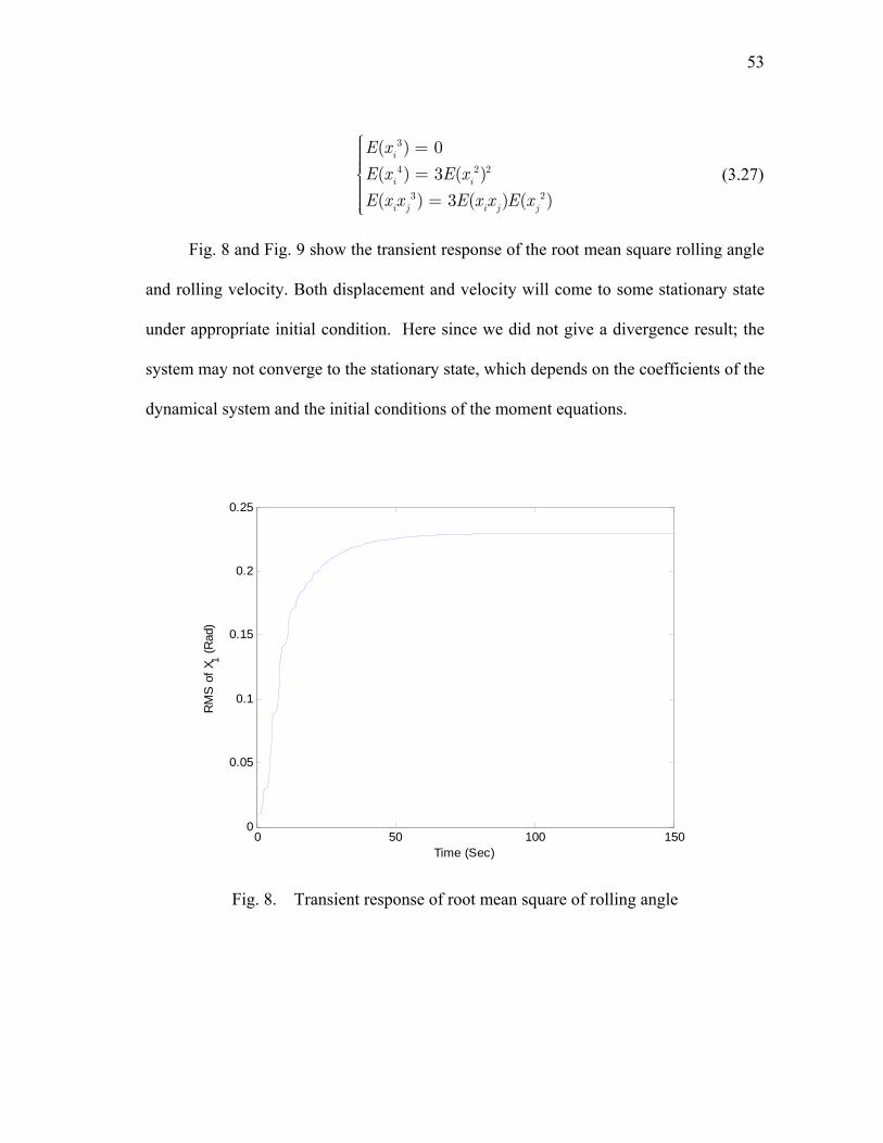
53

3

4 2 2

3 2

( ) 0

( ) 3 ( )

( ) 3 ( ) ( )

i

i i

i j i j j

E x

E x E x

E x x E x x E x

⎧⎪ =⎪⎪⎪ =⎨⎪⎪ =⎪⎪⎩

(3.27)

Fig. 8 and Fig. 9 show the transient response of the root mean square rolling angle

and rolling velocity. Both displacement and velocity will come to some stationary state

under appropriate initial condition. Here since we did not give a divergence result; the

system may not converge to the stationary state, which depends on the coefficients of the

dynamical system and the initial conditions of the moment equations.

Fig. 8. Transient response of root mean square of rolling angle

0 50 100 1500

0.05

0.1

0.15

0.2

0.25

Time (Sec)

RM

S o

f X1 (R

ad)

54

Fig. 9. Transient response of root mean square of rolling velocity

Fig. 10, Fig. 11 and Fig. 12 express the effect of the nonlinear damping

coefficient, nonlinear stiffness and linear damping on the rolling response. Horizontal

coordinates represent natural frequency of this dynamical system and vertical

coordinates represent stationary response of root mean square of rolling displacement.

Bending direction of the curves does not appear reasonable compared with some

conventional response amplitude curve with negative nonlinear stiffness, which bends to

the left. Some of the curves even have more than two values with respect to same

frequency, which is defined as a bifurcation phenomenon caused by nonlinearity of

0 50 100 1500

0.05

0.1

0.15

0.2

0.25

Time / (Sec)

RM

S o

f X2 (R

ad/s

)

55

dynamical system. Here we use 0ω (the undamped natural frequency of the dynamical

system)as the horizontal coordinate, and traditional amplitude curves are given by

0/ω ω , where ω represent the frequency of the harmonic excitation force and 0ω is

denominator there. So the stochastic response curves are still reasonable.

In Fig. 10, four different values of nonlinear damping coefficients were used. It is

expected that the response of the dynamical system should decrease with increasing

nonlinear damping. From Fig. 7, the excitation force spectrum has a peak frequency

close to 1.0 Rad/s. The maximum of response in Fig. 10 also appears in that range. This

can be viewed as a kind of ‘resonance’. The difference of response is limited when the

natural frequency 0ω is far from the peak frequency of excitation force or excitation

wave. Fig. 11 also adopts four different values of the nonlinear stiffness coefficient to

analyze the response, including the zero case and three negative values. There is a

significant difference in the low natural frequency range (left part of plot), compared to

Fig. 10, but limited difference in the high natural frequency domain. Fig. 12 shows the

effect of linear damping coefficient on the response curves. This result demonstrates one

peak value at some special frequency. Linear damping seems more important than the

nonlinear damping or stiffness coefficient comparing Fig. 10 and Fig. 11. By inspecting

the 27 moment equations up to second order, it seems impossible to analyze the

stochastic system by moment equation to above second order. There are 209 moment

equations for up to fourth order moments. In order to handle this difficulty, an automatic

neglect tool was designed and applied to the ship rolling motion to capture the response

of Non-Gaussian effect.

56

Fig. 10. Effect of nonlinear damping coefficient on the root mean square (RMS) of rolling displacement

Fig. 11. Effect of nonlinear stiffness coefficient on the root mean square (RMS) of rolling displacement

0.5 1 1.5 2 2.50

0.05

0.1

0.15

0.2

0.25

0.3

0.35

0.4

ω0

RM

S o

f X1 (R

ad)

δ3=0

δ3=0.03

δ3=0.06

δ3=0.12

0.5 1 1.5 2 2.50

0.05

0.1

0.15

0.2

0.25

0.3

0.35

0.4

ω0

RM

S o

f X1 (R

ad)

α3=0

α3=-0.44

α3=-0.88

α3=-1.0

57

Fig. 12. Effect of linear stiffness coefficient on the root mean square (RMS) of rolling displacement

3.2.2 The higher order cumulant neglect method with automatic neglect tool

In the cumulant closure technique, the response cumulants which are higher than

some closure level are assumed to be smaller in comparison to those cumulants below

the closure order and then can be neglected. To establish the relation between cumulants

and ordinary moments, we consider the random vector 1 1[ , ...... ]TnX x x x= with

characteristic function(Soong and Grigoriu, 1993) as follows.

11

( , , ) exp[ ]n

n i ii

u u E j u xφ=

⋅ ⋅ ⋅ = ∑ (3.28)

where 1j = − , n is the dimension of the state space in the diffusion process, e.g. in

equation (3.17), n=6. It can be expanded by Taylor series expansion in terms of ordinary

moments i jE x x ⋅ ⋅⋅ or cumulants , i jx xκ ⋅ ⋅⋅ . The expansion has two forms as follows

0.5 1 1.5 2 2.50

0.05

0.1

0.15

0.2

0.25

0.3

0.35

ω0

RM

S o

f X1 (R

ad)

μ=0.04μ=0.05

μ=0.1μ=0.15

58

2

1 11 1 1

1 1

( , , ) exp ( ) ( , )2!

( , , )!

n n n

n i i i j i ji i jn nC

i C i Ci C

ju u j u x u u x x

ju u x x

C

φ κ κ

κ

= = =

= =

⎧⎪⎪⋅ ⋅ ⋅ = + + ⋅ ⋅ ⋅⎨⎪⎪⎩⎫⎪⎪+ ⋅ ⋅ ⋅ ⋅ ⋅ ⋅ ⋅ ⋅ ⋅ + ⋅ ⋅ ⋅⎬⎪⎪⎭

∑ ∑∑

∑ ∑ (3.29)

2

2 11 1 1

1 1

( , , ) 1 ( ) ( )2!

( )!

n n n

n i i i j i ji i j

n nC

i j C i j Ci C

ju u j u E x u u E x x

ju u u E x x x

C

φ= = =

= =

⋅ ⋅ ⋅ = + + + ⋅ ⋅ ⋅

+ ⋅ ⋅ ⋅ ⋅ ⋅ ⋅ ⋅ ⋅ ⋅ + ⋅ ⋅ ⋅

∑ ∑∑

∑ ∑ (3.30)

here ‘C’ in equation (3.29)and (3.30) is the closure level and is a constant number. 1φ

and2φ are the same function with different expressions. Moments and cumulants can thus

be found through the characteristic functions.

1

1

1

11

1 0

1( )n

n

n

kk k

n k k kn u u

E x xj u u

φ

=⋅⋅⋅ =

∂⋅ ⋅ ⋅ =

∂ ⋅ ⋅ ⋅ ∂ (3.31)

1

1

1

21

1 0

ln1( , , )n

n

n

kk k

n k k kn u u

x xj u u

φκ

=⋅⋅⋅ =

∂⋅ ⋅ ⋅ =

∂ ⋅ ⋅ ⋅ ∂ (3.32)

where 1 2 nk k k k= + + ⋅ ⋅ ⋅ . Cumulants of order higher than the closure order ‘C’ can be

set equal to zero and moments higher than that closure order will be written in terms of

moments of order less than or equal to that closure level. The stochastic system equation

(3.17) has 6 state space variables, so n=6 in the characteristic function1φ and

2φ . The non-

Gaussian cumulant neglect method up to fourth order will involve 209 equations, which

is an extremely large, complex and nearly impossible system to find a solution to by

hand. The automatic procedure algorithm is described in Fig. 13. Compared with the

algorithm process in Wojtkiewicz’s dissertation (Wojtkiewicz, 2000), the algorithm

59

Fig. 13. Automatic Cumulant Neglect Tool procedure

1: Input System state space dimension ‘n’ and closure level ‘C’

2: Form the characteristic function in terms of cumulants (3.29) and moments(3.30) separately, both characteristic functions are truncated at closure level ‘C’.

3: Express all cumulants in equation (3.29) in terms of moments by equation(3.32).

4: Substitute all cumulants back to equation(3.29)

5: Determine those higher order response moments, which are above closure level, in terms of lower order moments by equation (3.31)

6: Form right hand side of equation (3.21) by substituting approximations for higher order moments in step 5

7: Write all moments equations achieved by last step into some ‘txt’ file and translate all moments equation to Matlab format for ‘ode’ solver

8: Matlab ‘ode’ solver to solve the ordinary differential equations

60

developed here takes advantage of two different expansions for the characteristic

function, i.e., equation (3.29) and (3.30). This avoids the difficulty of substitution

between the cumulants and the moments. Steps 1 to 7 generate the closed moment

equations using MAPLE and all moment equations are written into a ‘txt’ file and then

translated to the MATLAB format for the ‘ode’ solver in MATLAB. Step 8 takes

advantages of the efficiency and convenience of the MATLAB ordinary differential

equation solver.

3.2.2.1 Application to Stochastic Dynamical Systems with Analytical Solutions

Several precautions should be taken to the algorithm before programming the

tools in MAPLE and MATLAB. To reduce memory load and computational speed, the

symmetry of moments and cumulants require consideration to avoid repeating them. For

example, 1 2( )E x x and

2 1( )E x x are equivalent mathematically. In step 4, after substituting

all cumulants back into equation(3.29), the characteristic function 1φ is in terms of

moments with order less than or equal to closure level ‘C’.

Case 1

A simple Duffing oscillator with white noise excitation and nonlinear hardening

stiffness (Wojtkiewicz, 2000) is first analyzed to validate the accuracy of the automatic

neglect tool.

1 22 2 3

2 0 2 0 1 0 12 x x ( )

x x

x x W tζω ω εω

⎧ =⎪⎪⎨⎪ = − − − +⎪⎩ (3.33)

where ( )W t is a Gaussian white noise with zero mean and correlation:

1 2 2 1[ ( ) ( )] 2 ( ),EW t W t D t tδ τ τ= = − (3.34)

61

Parameters of the system are given by

00.1, 0.4, =0.2, 1Dε ζ ω= = = (3.35)

An analytical solution exists for the stationary probability density function of the system

defined in(3.33), which is given by

2 2 2 2 4

0 2 0 1 0 11 2 0

2( , ) exp( ( ))

2 2 4x x x

p x x CDζω ω εω

= − + + (3.36)

and 0C is the normalization constant, response moment can be easily calculated from this

analytical function. Fig. 14 indicates that the response has only one peak, as does a

Gaussian response.

Fig. 14. Analytical probability density function of unimodal Duffing oscillator

To verify the automatic neglect tool developed above, the mean square of displacement

is calculated and compared with the exact result from equation (3.36) and the numerical

-50

5

-5

0

50

0.05

0.1

0.15

0.2

x1x2

Pro

bability

Den

sity

Fun

ction

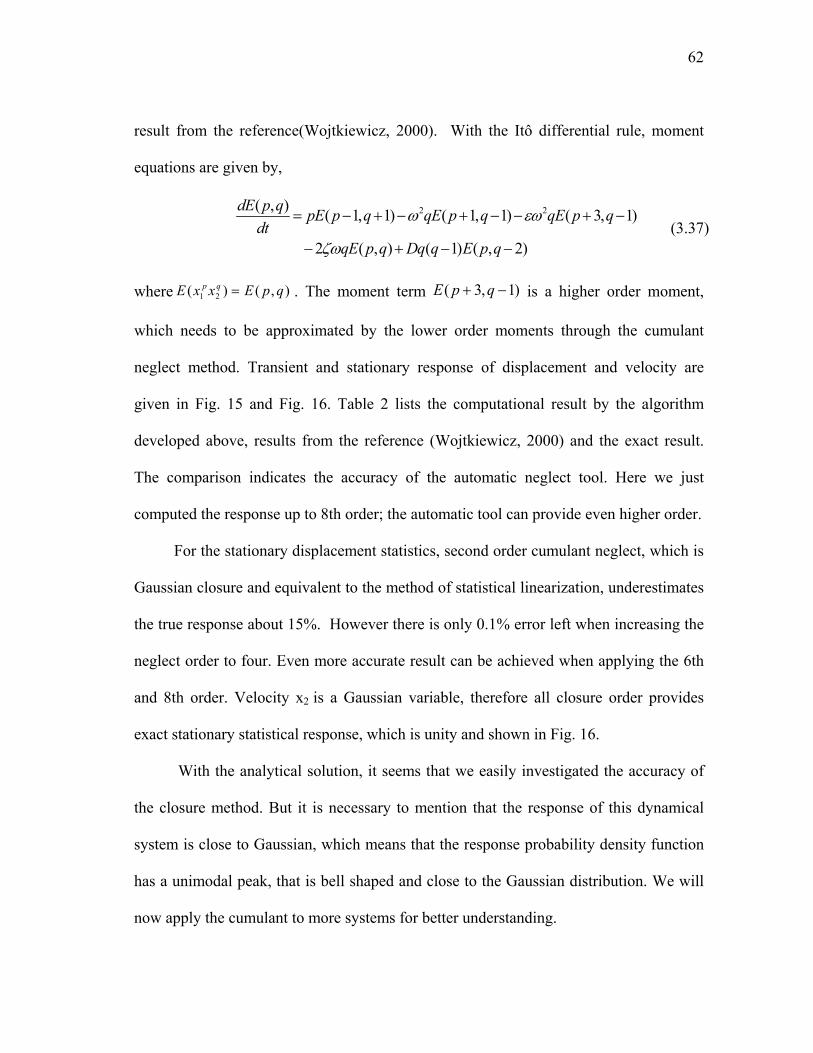
62

result from the reference(Wojtkiewicz, 2000). With the Itô differential rule, moment

equations are given by,

2 2( , ) ( 1, 1) ( 1, 1) ( 3, 1)

2 ( , ) ( 1) ( , 2)

dE p q pE p q qE p q qE p qdt

qE p q Dq q E p q

ω εω

ζω

= − + − + − − + −

− + − − (3.37)

where 1 2( ) ( , )p qE x x E p q= . The moment term ( 3, 1)E p q+ − is a higher order moment,

which needs to be approximated by the lower order moments through the cumulant

neglect method. Transient and stationary response of displacement and velocity are

given in Fig. 15 and Fig. 16. Table 2 lists the computational result by the algorithm

developed above, results from the reference (Wojtkiewicz, 2000) and the exact result.

The comparison indicates the accuracy of the automatic neglect tool. Here we just

computed the response up to 8th order; the automatic tool can provide even higher order.

For the stationary displacement statistics, second order cumulant neglect, which is

Gaussian closure and equivalent to the method of statistical linearization, underestimates

the true response about 15%. However there is only 0.1% error left when increasing the

neglect order to four. Even more accurate result can be achieved when applying the 6th

and 8th order. Velocity x2 is a Gaussian variable, therefore all closure order provides

exact stationary statistical response, which is unity and shown in Fig. 16.

With the analytical solution, it seems that we easily investigated the accuracy of

the closure method. But it is necessary to mention that the response of this dynamical

system is close to Gaussian, which means that the response probability density function

has a unimodal peak, that is bell shaped and close to the Gaussian distribution. We will

now apply the cumulant to more systems for better understanding.

63

Fig. 15. Mean square of displacement with different cumulant neglect order

Fig. 16. Mean square of velocity with different cumulant neglect order

0 5 10 15 20 25 30 35 400

0.1

0.2

0.3

0.4

0.5

0.6

0.7

0.8

0.9

Time

E(x

12 )

2nd Closure4th Closure6th Closure8th ClosureStationary Exact

0 5 10 15 20 25 30 35 400

0.2

0.4

0.6

0.8

1

Time

E(x

22 )

2nd Closure4th Closure6th Closure8th Closure

64

Table 2. Comparison of stationary mean square displacement of the

unimodal Duffing 0scillator

Closure Level

E(x12)

Result by Fig. 13

Result from (Wojtkiewicz,

2000) Error for E(x1^2)

Exact

Second Order Cumulant Neglect 0.805401 0.8054 1.49%

0.81756 Fourth Order Cumulant Neglect 0.816497 0.8165 0.13% Six Order Cumulant Neglect 0.817374 0.8174 0.02% Eighth Order Cumulant Neglect 0.817511 0.8175 0.01%

Case 2

To further investigate the application of the cumulant neglect method, we applied

the automatic tool to a four dimensional dynamical system(Er, 2000b), which will also

have a near Gaussian response with an analytical probability density function. It is

expected that the accuracy of response will increase with increasing of the closure order.

The four dimensional dynamical system is given by a two degree of freedom system:

3 5

1 1 11 1 2 12 2 3 1 4 1 5 1 1

3 52 1 2 12 1 22 2 6 2 7 2 8 2 2

1( 2 ) 2 4 6 ( )

21

[2(1 ) ] 2 4 6 ( )2

Y a s Y a s Y aY a Y aY W t

Y a a s Y s Y aY a Y a Y W t

⎧⎪⎪ + + + + + =⎪⎪⎨⎪⎪ + − + + + + =⎪⎪⎩

(3.38)

where 1, 2, 3, 8....a a a a are constant numbers and the white noises are defined by,

1 2 2 1[ ( ) ( )] ( ), , 1,2i j ijEW t W t s t t and i jδ τ τ= = − = (3.39)

The system is written in state space format as following:

65

1 2

3 52 1 11 2 2 12 4 3 1 4 1 5 1 1

3 4

3 54 1 2 12 2 22 4 6 3 7 3 8 3 2

1( 2 ) 2 4 6 ( )

2

1[2(1 ) ] 2 4 6 ( )

2

x x

x a s x a s x a x a x a x W t

x x

x a a s x s x a x a x a x W t

⎧ =⎪⎪⎪⎪⎪ =− + − − − +⎪⎪⎪⎨⎪ =⎪⎪⎪⎪⎪ =− − + − − − +⎪⎪⎩

(3.40)

where 1 1, 1 2, 2 3, 2 4,Y x Y x Y x Y x= = = =

Parameters are given as below,

1 3 4 5 7 6 8

11 22 12 2

a 1;a 1;a 1;a 0.5;a 0.5;a 1.5;a 0.2;

s 2; s 2; s , a arbitrary number

= = = = = = == = =

(3.41)

The analytical probability density function is given by (Scheurkogel and Elishakoff,

1988) with normalization constant.

2 2 2 4

1 2 3 4 1 2 4 3 1 4 1

6 2 4 65 1 6 3 7 3 8 3

1( , , , ) exp [ ( )

2]

p x x x x C a x x a x a x

a x a x a x a x

= − + + +

+ + + + (3.42)

The analytical equation (3.42) could be verified by substituting the PDF formula back to

the associated Fokker Planck Equation, equation(3.43),

3 51 11 2 2 12 4 3 1 4 1 5 1

2

1 2

3 51 2 12 2 22 4 6 3 7 3 8 3

4

3 42 2 2

11 22 122 22 42 4

1[[ ( 2 ) 2 4 6 ] ][ ] 2

1[[ [2(1 ) ] 2 4 6 ] ][ ] 2

1 12 2

a s x a s x a x a x a x px ppt x x

a a s x s x a x a x a x px px xp p p

s s sx xx x

∂ − + − − −∂∂= − −

∂ ∂ ∂

∂ − − + − − −∂− −

∂ ∂∂ ∂ ∂

+ + +∂ ∂∂ ∂ (3.43)

66

Fig. 17. Analytical probability density function of x1 x2 x3 and x4

The probability density function plots in Fig. 17 all have bell shaped curves for each

variable, which indicates that variables in this dynamical system may have Gaussian or

near Gaussian response. With the Itô differential rule, the moment equation is given by,

1 11

1 2 12 3

4 5

d (p, q, r, s)=p (p-1, q+1, r, s)+q(-(1 / 2)a s (p, q, r, s)

-a a s (p, q-1, r, s+1)-2a (p+1, q-1, r, s)

-4a (p+3, q-1, r, s)-6a (p+5, q-1, r, s))

+r (p, q, r-1, s+

E E E

E E

E E

E 1 2 12

1 22 6

7 8

11

1)+s(-a (1-a )s (p, q+1, r, s-1)

-(1 / 2)a s (p, q, r, s)-2a (p, q, r+1, s-1)

-4a (p, q, r+3, s-1)-6a (p, q, r+5, s-1))

+(1 / 2)s q(q-1) (p, q-2, r, s)

E

E E

E E

E

22 12 +(1 / 2)s s(s-1) (p, q, r, s-2)+s qs (p, q-1, r, s-1)E E

(3.44)

where 1 2 3 4(p, q, r, s)= ( )p p r sE E x x x x , there are four moments in the right hand side of

equation (3.44) which might need to be approximated by the cumulant neglect method

-4 -3 -2 -1 0 1 2 3 40

1

2

3

4

5

6

7

8

9

Varible limit

Pro

babi

lity

Den

sity

Fun

ctio

n

x1 PDF

x2 PDF

x3 PDF

x4 PDF

67

when the order is higher than the closure level, including (p+3, q-1, r, s)E ,

(p+5, q-1, r, s)E , (p, q, r+3, s-1)E , (p, q, r+5, s-1)E . As expected, the cumulant

neglect methods and moment equations successfully increase the accuracy of statistics of

the non Gaussian variables 1x and 3x by increasing the closure order in Fig. 18 and Fig.

19. Table 3 lists the error associated with the different closure level. We conclude that

the fourth order cumulant neglect method greatly reduces the error compared with the

Gaussian closure. Fig. 20 and Fig. 21 are the variances for velocities 2x , 4x , there is no

difference with increasing closure level, as the velocity variables are Gaussian

distributed.

Fig. 18. Mean square of x1 with different cumulant neglect order and exact solution

0 5 10 15 20 25 30 35 400

0.05

0.1

0.15

0.2

0.25

Time

E(x

12 )

2nd Closure4th Closure6th ClosureStationary Exact

68



0 5 10 15 20 25 30 35 400

0.05

0.1

0.15

0.2

0.25

Time

E(x

32 )


0 5 10 15 20 25 30 35 400

0.2

0.4

0.6

0.8

1

Time

E(x

22 )


69


Table 3. Comparison of stationary mean square of state variables with different closure level and exact stationary value

Closure Level

Stationary E(x1^2)

Error for E(x1^2)

Stationary E(x2^2)

Stationary E(x3^2)

Error for E(x3^2)

Stationary E(x4^2)

2nd Order 0.1789 12.99% 1.00 0.2021 7.34% 1.00 4th Order 0.1968 4.28% 1.00 0.2143 1.41% 1.00 6th Order 0.2014 2.04% 1.00 0.2164 0.39% 1.00

Exact 0.2056 1.00 0.2172 1.00

Case3

Both analytical solutions for case 1 and case 2 are close to the Gaussian distribution,

and cumulant neglect and moment equations perform excellently. In case 3, we will test

a simple one dimensional dynamical system with obvious non-Gaussian behavior.

0 5 10 15 20 25 30 35 400

0.2

0.4

0.6

0.8

1

Time

E(x

42 )


70

Considering the following stochastic differential equation with only additive noise (Er,

2000a):

3 5( ) / 2 ( )z z z z W tα= − − + (3.45)

where α is a constant and the Gaussian white noise is defined as

[ ( ) ( )] ( )EW tW t qτ δ τ+ = and q is also a constant. The analytical stationary PDF of z is

known to be

4 6

21( ) exp[ ( )]

2 2 3z z

p z c zq

α= − − (3.46)

wherec is the normalization constant. For α=0.05, q =2, the PDF is given in Fig. 22,

and the plot indicates that z is a non-Gaussian variable.

Fig. 22. Analytical probability density function of z

-5 -4 -3 -2 -1 0 1 2 3 4 50

0.05

0.1

0.15

0.2

0.25

0.3

0.35

z

Pro

babi

lity

Den

sity

Fun

ctio

n

71

The moment equations for the one dimensional system are derived following the Itô

differential rule, with ( ) ( )pE z E p= ,

( ) 1 1[ ( ) ( 2) ( 4)] ( 1) ( 2)

2 2dE p

p E p E p E p qp p E pdt

α= − + − + + − − (3.47)

The transient and stationary response of variance of zwith different closure level is in

given Fig. 23 and Table 4 shows that there is still 7.98% difference even with 10th order

cumulant neglect method, which could be explained by the plot in Fig. 22. The true

stationary response does not have a bell-shaped PDF, but two peaks.

Fig. 23. Mean square of z with different cumulant neglect order and exact solution

0 5 10 150

0.2

0.4

0.6

0.8

1

1.2

Time

E(z

2 )

2nd Closure4th Closure6th Closure8th Closure10th ClosureStationary Exact

72

Table 4. Comparison of stationary mean square of z with different closure level and

exact stationary value

Closure Level

Stationary E(z^2)

Error for E(z^2)

2nd Order 0.8883 25.32% 4th Order 1.0199 14.25% 6th Order 1.0645 10.50% 8th Order 1.0843 8.84%

10th Order 1.0945 7.98% Exact 1.1894

Case4

Case1, case2 and case3 only have additive excitation. We consider a dynamical

system with both multiplicative and additive stochastic noise, given in the following

equation,

2 51 2( ) ( ) ( ) ( )x x x x x x ax bx W t W tα η γ λ+ + + + = + + (3.48)

where 0, 0α η> > and 0ab > Gaussian white noise 1( )W t and 2( )W t are independent

with correlation function [ ( ) ( )] 2 ( ) ( 1,2)i i iiEW tW t K iτ π δ τ+ = = . The system

belongs to the generalized stationary potential when the following conditions are

satisfied (Lin and Cai, 2004):

2 21111

22

, ( )b K a K ba K

γ η α π= = + (3.49)

The stationary joint probability density function is given by equation (3.50) and the

marginal PDF is given in Fig. 24,

73

2 6

2 211 11 2 2 11 1

22

( , ) exp [ ]2 3K b x

p x x c x K abxK

α ππ λ

π+

= − + + (3.50)

where c is the normalization constant, and 1 2,x x x x= = . It is noted that the term

211 1K abxπ in the PDF equation is from the Wong-Zakai correction term due to the

parametric excitation. We assume 11 22 1/ (2 )K K π= = , 1.5η = , 1a bγ α λ= = = = = for

the computation.

Fig. 24. Analytical probability density function of x and x

The moment equations for the two dimensional system with multiplicative and additive

noise are derived following the Itô differential rule with Wong-Zakai correction terms,

2

2 2 211 11

222

( , ) ( 1, 1) ( ( , ) ( ( 2, )( , 2) 2 ( 1, 1) ( 5, 1)( ( 1, 1) ( , ))) ( 1)( ( 2, 2)

( , ) 2 ( 1, 1) ( 1) ( , 2))

dE p q pE p q q E p q E p qE p q E p q E p q

K a E p q b E p q K q q a E p q

b E p q abE p q K q q E p q

α η

γ γ λ

π π

π

= − + + − − +

+ + + + + − + −

+ + − + + − + −

+ + + − + − −

(3.51)

-3 -2 -1 0 1 2 30

0.1

0.2

0.3

0.4

0.5

0.6

0.7

Variable Displacement and Velocity

Pro

bability

Den

sity

Fun

ction

DisplacementVelocity

74

where 1 2(p, q)= ( )p pE E x x The marginal PDF of displacement and velocity in Fig. 24

have Gaussian or nearly Gaussian response, it is expected that cumulant neglect method

with moment equation will give more accurate solution with neglect order increasing.

Second to sixth order closure are applied to the parametric system, Fig. 25 and Fig. 26

display the evolution to stationary statistics for both displacement and velocity. As

discussed in the previous cases, the velocity variable is Gaussian distributed, so all

different closure gives same solution. While the displacement is a non Gaussian variable,

the higher order closure predicts a better estimation. However, instability happens when

increasing the closure order to eight as shown in Fig. 27 and Fig. 28. The question is

whether this instability is just a mathematical error or mistakes from the methodology.

Further research is necessary to address this problem.

Fig. 25. Mean square of 1x with different cumulant neglect order and exact solution

0 5 10 15 20 25 30 35 40 45 500

0.05

0.1

0.15

0.2

0.25

0.3

0.35

Time

E(x

12 )


75


Table 5. Comparison of stationary mean square of 1x and 2x with different closure level

and exact stationary value

Closure Level

Stationary E(x1^2)

Error for E(x1^2)

Stationary E(x2^2)

Error for E(x2^2)

2nd Order 0.2419 19.34% 0.3333 0.00% 4th Order 0.2758 8.04% 0.3333 0.00% 6th Order 0.2865 4.47% 0.3333 0.00%

Exact 0.2999 0.3333

0 5 10 15 20 25 30 35 40 45 500

0.05

0.1

0.15

0.2

0.25

0.3

0.35

Time

E(x

22 )


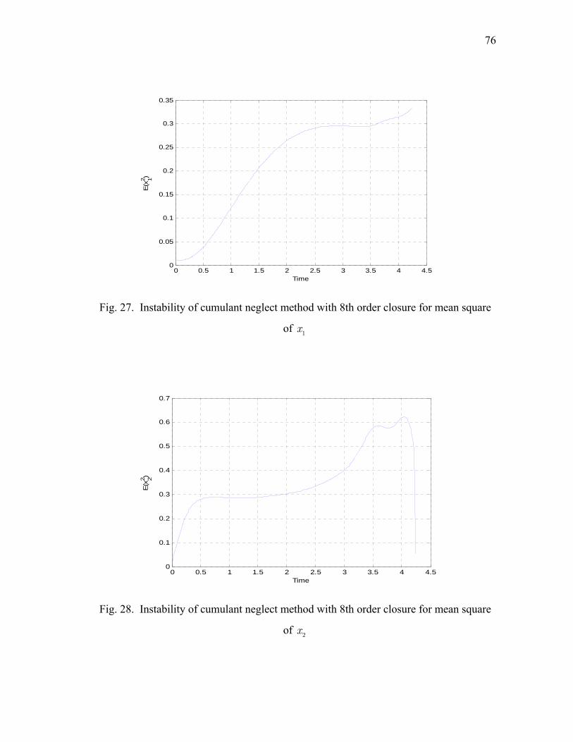
76

Fig. 27. Instability of cumulant neglect method with 8th order closure for mean square

of 1x

Fig. 28. Instability of cumulant neglect method with 8th order closure for mean square

of 2x

0 0.5 1 1.5 2 2.5 3 3.5 4 4.50

0.05

0.1

0.15

0.2

0.25

0.3

0.35

Time

E(x

12 )

0 0.5 1 1.5 2 2.5 3 3.5 4 4.50

0.1

0.2

0.3

0.4

0.5

0.6

0.7

Time

E(x

22 )

77

Case5

The bimodal Duffing oscillator was considered to investigate the limitation of

cumulant neglect method (Wojtkiewicz, 2000). The stochastic dynamical system is

given by

1 22 2 3

2 0 2 0 1 0 12 x x ( )

x x

x x W tζω ω εω

⎧ =⎪⎪⎨⎪ = − + − +⎪⎩ (3.52)

The only difference from case1 is the negative linear stiffness. All parameters are same

with the dynamical system defined in equation(3.33). Analytical joint probability density

function is given by below equation and plotted in Fig. 29 and Fig. 30, which indicates

that the response has obviously double peaks, thus non-Gaussian behavior,

2 2 2 2 4

0 2 0 1 0 11 2 0

2( , ) exp( ( ))

2 2 4x x x

p x x CDζω ω εω

= − − + (3.53)

The cumulant neglect applications with different closure order (2nd to 6th order) are

displayed in Fig. 31, Fig. 32 and Table 6. Since velocity is a Gaussian variable, all level

closure provides the exact result. But the accuracy for displacement variable is much

less attractive; there is very limited progress with higher order neglect method. The

performance of 8th order neglect method is same as the previous example; further

research is needed to understand the instability of the algorithm.

78

Fig. 29. Analytical probability density function of bimodal Duffing oscillator

Fig. 30. Marginal probability density function of Duffing oscillator

-10-5

05

10

-10-5

0

5100

5

10

15


Pro

babi

lity

Den

sity

Fun

ctio

n

-10 -8 -6 -4 -2 0 2 4 6 8 100

0.05

0.1

0.15

0.2

0.25

0.3

0.35

0.4

Variable Displacement and Velocity

Pro

babi

lity

Den

sity

Fun

ctio

n


79



0 5 10 15 20 25 30 35 40 45 500

1

2

3

4

5

6

7

8

9

Time

E(x

12 )

2nd closure4th closure6th closureStationary exact

0 5 10 15 20 25 30 35 40 45 500

0.5

1

1.5

2

2.5

Time

E(x

22 )


80

Table 6. Comparison of stationary mean square of 1x and 2x with different closure level

and exact stationary value for bimodal Duffing oscillator

Closure Level

Stationary E(x1^2)

Result from (Wojtkiewicz,

2000) Error for E(x1^2)

Stationary E(x2^2)

Error for E(x2^2)

2nd Order 4.1387 4.1387 52.50% 1.000 0.00% 4th Order 5.0000 5.0000 42.62% 1.000 0.00% 6th Order 5.3195 5.3196 38.95% 1.000 0.00%

Exact 8.7136 1.000

Fig. 33. Instability of cumulant neglect method with 8th order closure

for mean square of 1x

0 5 10 15 20 25 300

5

10

15

20

25

30

35

40

Time

E(x

12 )

81

Fig. 34. Instability of cumulant neglect method with 8th order closure

for mean square of 2x

3.2.2.2 Application to Rolling motion with Filter

By applying the automatic cumulant neglect tool, the moment equations for the

stochastic system (3.17) up to fourth order have been computed to compare with

Gaussian neglect result in last section. The moment equation is derived as below,

320

3

2

( , , , , , ) ( 1, 1, , , , ) (2 ) ( , , , , , )

( , 2, , , , ) ( 1, 1, , , , )

( 3, 1, , , , ) ( , 1, 1, , , )

( , , 1, 1, , ) ( , , , 1, 1, )

( , , 1,

dE p q r s t m pE p q r s t m q r E p q r s t m

qE p q r s t m qE p q r s t m

qE p q r s t m qE p q r s t m

rE p q r s t m sE p q r s t m

sE p q r s

μ λδ ωα ε

λ

= − + − +

− + − + −− + − + − ++ − + + − +− + −

1 02

3

1, , ) ( , , , , 1, 1)

( , , 1, , 1, ) ( , , 1, , , 1)

( 1) ( , , , 2, , )

t m tE p q r s t m

tE p q r s t m mE p q r s t m

s s E p q r s t m

λ λπγ

+ − +− + − − + −

+ − −

(3.54)

0 5 10 15 20 25 30-40

-30

-20

-10

0

10

20

30

Time

E(x

22 )

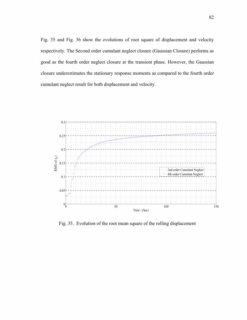
82

Fig. 35 and Fig. 36 show the evolutions of root square of displacement and velocity

respectively. The Second order cumulant neglect closure (Gaussian Closure) performs as

good as the fourth order neglect closure at the transient phase. However, the Gaussian

closure underestimates the stationary response moments as compared to the fourth order

cumulant neglect result for both displacement and velocity.

Fig. 35. Evolution of the root mean square of the rolling displacement

0 50 100 1500

0.05

0.1

0.15

0.2

0.25

0.3

Time / (Sec)

RM

S of

x 1)

2nd order Cumulant Neglect4th order Cumulant Neglect

83

Fig. 36. Evolution of the root mean square of the rolling velocity

3.3 Discussions of the Moment Equations

Due to the complications of higher dimensional stochastic systems, this dissertation

develops a convenient method of analyzing these higher dimensional systems. The

higher order moment equations are solved with a cumulant neglect method with an

automatic neglect tool. This algorithm will greatly assist in analyzing higher dimensional

stochastic dynamical systems at any closure level. And kurtosis could be verified larger

than 3 by checking fourth order moments, which shows non Gaussian effect of rolling

motion response and soft spring effect (Winterstein, 1988).

As analyzed in the case 4, a system with parametric stochastic excitation

(multiplication noise) can be analyzed as well as external stochastic excitation (additive

noise) without loss of generality. The mathematical model for ship rolling here is an

approximate frequency domain equation. Constant coefficients are used for the added

0 50 100 1500

0.05

0.1

0.15

0.2

0.25

Time / (Sec)

RM

S of

x 2

2nd order Cumulant Neglect4th order Cumulant Neglect

84

mass and added damping. All these coefficients are selected with respect to the peak

frequency of the excitation force and within frequency domain analysis. Following

Ogilvie (Ogilvie, 1964), the modified time domain rolling equation with impulse

response function is derived and analyzed using an extended state space method

(Holappa and Falzarano, 1999). Instead of numerical simulation, the extended state

space system can be studied in a stochastic conception. With the extended state space,

time domain state space model will become more complicated, but the automatic tool

developed in this dissertation will be able to handle the high dimensional stochastic

system without difficulty. Additionally, all linear filter variables and extended state

space variables (if extended by linear system) are all Gaussian variables, thus only

Gaussian cumulant neglect method (second order) is needed to cut off those variables

associated moment equations. This will largely reduce the amount of moment equations.

With the automatic cumulant neglect tool, we should be able to calculate the

response moment with arbitrary number of states and closed at any closure level

theoretically. However, the cumulant neglect method provides good approximation only

when the response of systems is close to Gaussian behavior. If the system posses any

jump behavior, e.g. bimodal oscillator in case 5, the cumulant neglect method is not

capable to capture the true displacement moments. Also the higher order moment

equations involves many ordinary differential equations even for the low dimensional

dynamical system, time domain simulation of those closed moment equations is

necessary for stationary statistics. Therefore it is difficult to find any moment jump

phenomena.Equation Section (Next)

85

CHAPTER IV

MARKOV AND MELNIKOV BASED APPROACHES FOR

STABILITY ANALYSIS

Vessel stability or capsizing analysis in random beam sea has been approached

using different analytical methods in the past decades. However, due to the strong

softening nonlinear stiffness and stochastic excitation, there is still no general method of

dealing with capsizing prediction in a random sea. The Fokker-Planck Equation (FPE)

based on the continuous Markov process model and the phase space flux rate based on

Melnikov function are two of the most attractive analytical approaches which provide

different views of the capsizing criteria. In this chapter, both methods have been applied

to the same vessel model to compare its capabilities and efficiencies and also discussed

their limitations and advantages for capsizing criterion development. In the Markov

based portion, both the shaping filter method and the stochastic averaging of energy

envelope are applied to the SDOF freedom rolling equation. The rate of phase transport

flux based on the Melnikov function and the mean first passage rate based on FPE are

compared for capsizing prediction. The relationship, i.e., similarities and differences

between the two is then demonstrated through various parameter studies.

86

4.1 Introduction

Stochastic analysis of nonlinear marine structures is used to examine the random

response and stability of the ocean system. Ship rolling is the most typical strong

nonlinear phenomena in ocean engineering. All our cases are based on the ship rolling

problem in the beam seas. However all methods mentioned and studied here could be

applied to other nonlinear stochastic problems without loss of generality. Two different

approaches are applied to the dead ship (zero speed) condition with random beam waves,

the so called Markov and the Melnikov based method.

A random process can be recognized as a Markov process if its future probability

depends only on its most recent values. The Fokker Planck equation (FPE) is the related

equation governing probability density function of the system response distribution of a

Markov process. The FPE is a partial differential equation with appropriate initial and

boundary condition discussed in the second Chapter. When the system is excited by

purely Gaussian white noise, the response will be a Markov process and the probability

density function is governed by the FPE. Unfortunately, the wave excitation is described

by a non-white spectrum or even a narrow banded spectrum. The FPE cannot be applied

to the rolling motion directly. Basically, researchers found two different ways to

overcome this difficulty by using a shaping filter (Francescutto and Naito, 2004; Su and

Falzarano, 2011) or stochastic averaging of energy envelope of response (Roberts, 1982;

Roberts and Vasta, 2000). By applying the shaping filter technique, any wave excitation

spectrum can be generated from the designed filter. When the dynamical system with

filter variables are written into the Itô type differential equation, the related FPE

87

equation gives the transition probability density function with higher dimensions. The

difficulty is solving the higher dimensional FPE. It should be noted that many

researchers are still working on solving the higher dimensional FPE (Naess and Moe,

2000; Di Paola and Sofi, 2002; Kumar et al., 2010; Er, 2011; Martens and Wagner,

2011). The solution to the FPE is the transition probability density function of the

response. The first passage type failure could be easily solved by defining the reliability

function with transient probability density function. In this chapter, we do not focus on

solving the FPE numerically due to its difficulty and efficiency. The Automatic neglect

cumulant neglect tools was developed in the Chapter three to analyze the higher

dimensional stochastic dynamical system approximately, but it is still far from

satisfactory for capsizing analysis. Alternatively, stochastic averaging of the energy

envelope was applied to analyze rolling motion by Roberts (Roberts, 1982; Roberts and

Vasta, 2000). By reducing the dimension of the dynamical system to one dimension, the

first passage time could be derived from the well-known Pontryagin equation (Andronov

et al., 1933). And the first passage time is defined as the capsizing criterion based on the

Markov method. The limitation of the stochastic averaging method is that the input

spectrum bandwidth has to be much wider than the output spectrum bandwidth. Only

when the damping is very light, can this condition be met.

As a global geometric method, the Melnikov method was introduced to naval

architecture, ship rolling in harmonic waves by Falzarano (Falzarano, 1990; Falzarano et

al., 1992). The method has already been applied to the rolling problems with stochastic

excitation (Hsieh et al., 1994; Jiang et al., 2000; Vishnubhotla et al., 2000; Falzarano et

88

al., 2010). Ship capsizing is described in the phase space plane by the escape of a

trajectory from the safe basin or potential well to the unsafe area under random

excitation. The normalized phase transport rate or phase flux rate was defined as a

criterion for vessel capsizing analysis.

We applied both the Markov and the Melnikov method to the same vessel

parameters in this chapter to compare their relative efficiency and discuss their

advantages and disadvantages.

4.2 Markov Modeling for Capsizing Analysis

Markov modeling of the stochastic dynamical system is based on the diffusion

process. The general theory requires that the excitation force has to be a pure white noise

process, while the random wave excitation spectrum normally has a limited bandwidth

and a peak value. Basically, there are two different ways to deal with this problem. The

first method is using a shaping filter to extend the two dimensional dynamical system to

a higher order system by increasing the number of state space filter variables. The

second is using the stochastic averaging of the energy envelope of the response by

reducing the dimension of the stochastic system. Both methods are based on Markov

process.

The shaping filter method was introduced in chapter III. Numerical solution of the

FPE for high dimensional stochastic dynamical system always involves convergence and

accuracy issues. Even if it is possible, it will be difficult. As an alternative analytical

method introduced in the third Chapter, the Moment equation, which governs the

89

response of statistical moments, can be solved after applying some reasonable

assumptions and closure technique. There is no small perturbation parameters

assumption in the shaping filter model. By increasing additional filter dimensions, the

difficulty of the shaping filter model is how to accurately estimate the probability density

function of the stochastic dynamical systems. Once the solution of the FPE is given, the

reliability function, the first passage time distribution and the mean first passage time

will be easily calculated based on the Kolmogorov backward equation(Lin and Cai,

2004).

4.2.1 Energy based stochastic averaging

Instead of increasing the dimensions, stochastic averaging of the energy envelope

enables the two dimensional rolling model to be reduced to a one dimensional problems

for the system energy, which can be modeled approximately as a continuous one

dimensional Markov process. This approach has been applied to ship rolling analysis for

decades (Roberts, 1982; Roberts, 1986; Roberts and Spanos, 1986; Roberts and Vasta,

2000; Roberts and Vasta, 2000; Roberts and Vasta, 2001; Roberts and Vasta, 2002). The

capsizing phenomenon is considered as a first passage type problem. Mean first passage

time to reach a critical energy level can be evaluated from the associated FPE of the

Markov process.

4.2.1.1 Rescaling of the roll equation of motion

For analytical convenience, the single degree of freedom roll equation can be

non-dimensionalized to (Roberts, 1986),

90

31 2( ) ( ) ( ) ( ) ( ) ( ) ( )x b x b x x x x Fτ τ τ τ τ τ τ+ + + − = (4.1)

where the non-dimensionalized coefficients are defined as below

** 11 3

44 44

444

4

41 2 *

1 4 44 1

/ , ,( )

( )(

/ ,

( )) ( )

, , ( )

n n

qn

CC C x t

I ABB f t

b b FC CI A

φ φφ τ ω ωω

ωωω

ωτ

φ+

Δ= = = =

+

= = =Δ Δ

(4.2)

It is noted that the nonlinear coefficient of stiffness has been non-dimensionalized to

unity for convenience, but it is not necessary. Also the wave excitation force can be

assumed as a stationary Gaussian stochastic process with zero mean and its spectrum can

be defined as

* 21

1( ) ( ) / ( ) ( )cos( )

2FF ffS S C R v v dvω φπ

∞

−∞Ω = Δ = Ω∫ (4.3)

( ) [ ( ) ( )]R v F F vτ τ= Ε + (4.4)

( )R v is the auto covariance function of ( )F τ and frequency / nω ωΩ = is the non-

dimensional frequency. [ ]Ε i is expectation operator. The physical meaning of ( )ffS ω and

( )rollingF ω are defined in chapter three. In this chapter, ( )Sηη ω is represented by the ISSC

(International Ship Structure Congress) two parameter spectral formula given by

4

2 45

( ) 0.11 exp( 0.44( ) )z zsS Hηη

ω ωω

ωω= − (4.5)

In the non-dimensionalized rolling model, we have only four parameters, linear damping

1b , nonlinear damping2b , significant wave height

sH and characteristic wave frequency

91

zω . Both the Markov and Melnikov based approaches will be applied to analyze the

effects of these four parameters.

The damping coefficients for rolling are small compared with the stiffness

coefficients. For convenience in the derivation of the theory, equation (4.1) is rescaled

using the perturbation parameter ε as followed,

2 22 3

1 2( ) ( )( ( ) ) ( ) ( ) ( )x x b b x x x Fεε ετ ε τ τ τ τ ε τ+ + + − = (4.6)

where 22

11b b

εε = , 2

222

b bε

ε = and ( ) ( )F Fεε τ τ= . The scaling parameters ε is used here

help to indicate the order of magnitude of the damping and excitation terms. The scaling

of the excitation ensures that the standard deviation of the response is of order 0ε as

0ε → but this does not imply that the excitation is weak in an absolute sense (Roberts

and Vasta, 2001).The total energy envelope process ( )E τ of the oscillator is defined as:

2

( ) ( )2x

E V xτ = + (4.7)

where 0

( ) ( )x

V x k dξ ξ= ∫ , and 3( )k x x x= − is the softening stiffness and the total

energy consists of the kinetic energy and the potential energy. In the absence of input

noise excitation and dissipation, the quantity of ( )E τ is conserved. This implies that the

Hamiltonian system is integrable. It is possible to define ( )E τ and phase angle ( )τΦ to

rewrite the rolling equation followings (Roberts and Vasta, 2002):

sgn( ) ( ) cosx V x E= Φ (4.8)

2 sinx E=− Φ (4.9)

92

The variable transformation gives two first order ordinary differential equation for ( )E τ

and ( )τΦ independently.

2

1 12

22

( )( )

( )

EFε

τ ε α εβτ

εβτ ε α γ

⎛ ⎞⎡ ⎤ ⎡ ⎤− ⎟⎜⎢ ⎥ ⎢ ⎥⎟⎜= +⎟⎜⎢ ⎥ ⎢ ⎥⎟Φ − + ⎟⎜⎝ ⎠ ⎢ ⎥⎢ ⎥ ⎣ ⎦⎣ ⎦ (4.10)

where,

21 2 sinEhα = Φ (4.11)

2 sin coshα = − Φ Φ (4.12)

1 2 sinEβ = − Φ (4.13)

2 cos / 2Eβ = − Φ (4.14)

( , ) / ( , )k E V Eγ = Φ Φ (4.15)

2 21 2( )h b b x

ε ετ= + (4.16)

4.2.1.2 The Markov process approximation

The Markov process of the energy ( )E τ is approximated by a one dimensional

stochastic Itô differential equation:

( ) ( ) ( )dE m E dt D E dBτ = + (4.17)

/ ( )dB d Wτ τ= and ( )W τ is the Gaussian white noise excitation. ( )B τ is defined as a

Wiener or Brownian process. ( )m E and ( )D E are defined as the drift and diffusion

coefficients and are estimated from the known coefficients in equation(4.1). The FPE

equation associated with (4.17) is given by:

93

20 0

0 0 0 02

( , | , ) 1( ( ) ( , | , )) ( ( ) ( , | , ))

2p E E

m E p E E D E p E EE E

τ ττ τ τ τ

τ∂ ∂ ∂

= − +∂ ∂ ∂

(4.18)

0( | , )p E E τ is the transition probability density function of the oscillator energy. For this

one dimensional partial differential equation, a numerical solution is possible to be

calculated. Also an analytical solution of stationary response is given in (Roberts and

Vasta, 2000).

There are two alternative ways to derive the drift and diffusion coefficients and

they are explained by Roberts in two separate papers (Roberts, 1982; Roberts and Vasta,

2000). The old theory is based on Stratonovich-Khasminskii (SK) limit theorem

(Stratonovich, 1963; Khasminskii, 1966). The new derivation is based on physical

reasoning, which gives a correction term to the drift coefficients. A fundamental

assumption of the Markov model iscorrτ τΔ > , where

corrτ is the correlation time scale

of the excitation and τΔ is that the time step for energy increment. If the damping is

sufficiently small, then this condition can be met. If the bandwidth of the excitation

increases, and the correlation time reduces, then the restriction on the magnitude of

damping reduces (Roberts and Vasta, 2000). Define ( ) ( ) ( )E E Eτ τ τ τΔ = +Δ − ,the

drift coefficient ( )m E and drift coefficient ( )D E are given by

1( ) [ ]m E E

τ= ΕΔ

Δ (4.19)

21( ) [( ) ]D E E

τ= Ε Δ

Δ (4.20)

These two coefficients are approximated by a perturbation to the free and undamped

oscillation. It is necessary to find the solution for the undamped, unforced oscillator:

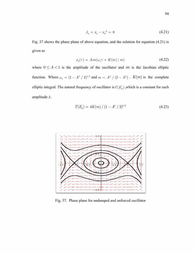
Fig

giv

wh

fun

elli

am

g. 37 shows

ven as

here 0 A≤ <

nction. Whe

iptic integral

mplitudeA .

the phase pl

1< is the

ere 1 (1ω = −

l. The natura

Fig. 37. Ph

0x +

lane of abov

0( )x Aτ =

amplitude o

2 1/2/ 2)A−

al frequency

0( ) 4T E =

hase plane fo

30 0x x+ − =

ve equation,

1(Asn Kω τ +

of the oscill

and m A=

y of oscillato

4 ( ) / (1K m −

r undamped

0=

and the solu

( ) | )K m m

lator and sn

2 2/ (2 )A−

r is0( )T E ,w

2 1/2/ 2)A−

d and unforce

ution for equ

n is the Ja

. ( )K m is

which is a co

ed oscillator

(4.2

uation (4.21)

(4.2

acobian ellip

the compl

onstant for ea

(4.2

94

21)

) is

22)

ptic

lete

ach

23)

95

The dissipation terms in equation (4.10)1α and

2α can be averaged over the period of the

unforced undamped oscillation 0( )T E by treatingE as a constant over one period and

0Φ = Φ .

2

1 12

22

( )( )

( )

EFε

τ ε εβτ

εβτ ε γ

⎛ ⎞⎡ ⎤ ⎡ ⎤− Λ ⎟⎜⎢ ⎥ ⎢ ⎥⎟⎜= +⎟⎜⎢ ⎥ ⎢ ⎥⎟Φ − Λ + ⎟⎜⎝ ⎠ ⎢ ⎥⎢ ⎥ ⎣ ⎦⎣ ⎦ (4.24)

21 0

0

2sin

( )E

h dtT E

Λ = Φ∫ (4.25)

2 0 00

1sin cos

( )h dt

T EΛ = − Φ Φ∫ (4.26)

By using the drift and diffusion definitions given by equation (4.19) and (4.20), and the

first row of equation (4.24), ( )m E and ( )D E can be obtained by following (Roberts and

Vasta, 2000; Roberts and Vasta, 2002):

2 2 21

1,2...

1( ) ( ) ( ) ( ( ))

2 n n FFn

m E E s c S n Eε π ω∞

=

= − Λ + +∑ (4.27)

2

1,2...

( ) 2 ( ( ))n FFn

D E E s S n Eπ ω∞

=

= ∑ (4.28)

where,

00

1

( )sin sin( ( ))

2n

n

xs n E

E

τω

∞

=

Φ = − = ∑ (4.29)

0 00

1

sgn( ) ( )cos cos( ( ))n

n

x V xc n E

Eω

∞

=

Φ = = ∑ (4.30)

The derivation of drift and diffusion coefficients can be found in the Appendix B. Fig.

38 to Fig. 40 demonstrated the Fourier expansion of 0sin Φ and

0cosΦ . At low energy

96

level, like Fig. 38, the coefficients of the expansion can be cut off at 1, which already

gives a good approximation. However, when the system goes up to a higher energy orbit,

Fig. 39 indicates the Fourier coefficients are not sufficient to provide a good

approximation. While Fig. 40 gives an excellent estimation when the summation in

equation (4.29) and (4.30) are truncated at n=5. A truncation order at n=5 will be

adopted in the following computations.

The drift and diffusion coefficients are depicted in Fig. 41 and Fig. 42 with a

varying excitation force and the same characteristic wave frequency 2 / 9zω π= . It is

clear to see that both the drift and diffusion coefficients will increase with increasing of

excitation force. Fig. 43 and Fig. 44 demonstrate the effect of the characteristic wave

frequency zω on the drift and diffusion coefficients. It is interesting to observe that

2 / 5zω π= gives a very large value of drift and diffusion coefficients at the low

energy level. The reason is ( ) 1Eω → as 0E approach to zero,

1s and 1c is the

dominant value for ns and

nc , so ( / 1)FF nS ω ωΩ = = will be dominant for ( )m E and

( )D E . Based on the numerical testing, the frequency of the peak value of ( )FFS Ω will be

close to 1, as 2 / 4zω π→ . This effect can be considered as kind of ‘stochastic

resonance’. The damping coefficients effect on the drift coefficient are demonstrated at

Fig. 45 and Fig. 46, it is expected that the larger damping will give a larger negative

effect on drift value. The diffusion coefficients are not affected by the damping

coefficients based on equation(4.28).

97


0cosΦ at 0E =0.01 and n=1


0cosΦ at 0E =0.2499 and n=1...3

0 1 2 3 4 5 6 7-1

-0.8

-0.6

-0.4

-0.2

0

0.2

0.4

0.6

0.8

1

Time/τ

Val

ue o

f sin

Φ0 a

nd c

osΦ

0

sinΦ0

Fourier expansion of sinΦ0

cosΦ0

Fourier expansion of cosΦ0

0 2 4 6 8 10 12 14 16 18-1.5

-1

-0.5

0

0.5

1

1.5

Time/τ

Val

ue o

f sin

Φ0 a

nd c

osΦ

0

sinΦ0


cosΦ0


98


0cosΦ at 0E =0.2499 and n=1...5

Fig. 41. Drift coefficients for varioussH , Unit: Meter

0 2 4 6 8 10 12 14 16 18-1.5

-1

-0.5

0

0.5

1

1.5

Time/τ

Val

ue o

f sin

Φ0 a

nd c

osΦ

0

sinΦ0


cosΦ0


0 0.05 0.1 0.15 0.2 0.25-0.01

-0.005

0

0.005

0.01

0.015

0.02

0.025

E0

m(E

)

Hs=1Hs=5Hs=9Hs=13

99

Fig. 42. Diffusion coefficients for varioussH , Unit: Meter

Fig. 43. Drift coefficients for variouszω ,

sH =5m

0 0.05 0.1 0.15 0.2 0.250

0.002

0.004

0.006

0.008

0.01

0.012

0.014

0.016

0.018

E0

D(E

)

Hs=1Hs=5Hs=9Hs=13

0 0.05 0.1 0.15 0.2 0.25-8

-6

-4

-2

0

2

4

6x 10-3

E0

m(E

)

ωz=2π/2

ωz=2π/5

ωz=2π/8

ωz=2π/11

ωz=2π/14

100

Fig. 44. Diffusion coefficients for variouszω ,

sH =5m

Fig. 45. Drift coefficients for various linear damping coefficients1b ,

sH =5m,

2 / 9zω π=

0 0.05 0.1 0.15 0.2 0.250

0.5

1

1.5

2

2.5

3

3.5

4x 10-3

E0

D(E

)

ωz=2π/2

ωz=2π/5

ωz=2π/8

ωz=2π/11

ωz=2π/14

0 0.05 0.1 0.15 0.2 0.25-6

-5

-4

-3

-2

-1

0

1x 10-3

E0

m(E

)

b1=0

b1=0.005

b1=0.01

b1=0.015

b1=0.02

101

Fig. 46. Drift coefficients for various nonlinear damping coefficients2b ,

sH =5m

2 / 9zω π=

4.2.2 First passage failures

The one dimensional Markov model equation (4.17) derived before can be easily

applied to study the first passage problem. We are concerned with the random time FPST

when the Markov processE first cross the critical boundary valuecE , given the condition

that0 0( )E Eτ = , where

0 cE E< and cE corresponds to an absorbing boundary. We

assume 0 0( , | , )p E Eτ τ to be the transition probability density of the Markov process

( )E τ . The reliability function0 0( , ; , )cR E Eτ τ , which is defined as the probability of

( )l cE E Eτ≤ < at timeτ , where lE is the lower bound and is a non-critical boundary.

0 0.05 0.1 0.15 0.2 0.25-4

-3

-2

-1

0

1

2

3x 10-3

E0

m(E

)

b2=0

b2=0.015

b2=0.03

b2=0.045

b2=0.06

102

0 0 0 0 0 0 0

0

( , ; , ) ( , | , ) [ | ( ) ]

( ) ,

c

l

E

c FPS

E

l c

R E E p E E d ProbT E E

E E E

τ τ τ τ τ τ τ τ

τ τ τ

= = > − =

≤ < ≥

∫ (4.31)

If equation (4.18) can be solved for0 0( , | , )p E Eτ τ , the reliability function can be

determined by integrating equation (4.31). Also, reliability function satisfies the

Kolmogorov backward equation (Lin and Cai, 2004):

2

0 0 20 0

1( ) ( ) 0

2FPS

R R Rm E D E

E Eτ∂ ∂ ∂

− + + =∂ ∂ ∂

(4.32)

where 0FPSτ τ τ= − is the first passage time. Equation (4.32) can be solved given

initial and boundary condition. Probability distribution function of first passage time

FPST is given by

0 0( ) [ | ( ) ] 1 ( )FPST FPS FPS FPS FPSF ProbT E E Rτ τ τ τ= < = = − (4.33)

The probability density function of FPST is given by

( ) ( ) ( )FPS FPST FPS T FPS FPS

FPS FPS

p F Rτ τ ττ τ∂ ∂

= = −∂ ∂

(4.34)

The moments of first passage time FPST satisfy the generalized Pontryagin equation (Lin

and Cai, 2004).nM is the nth moment of the first passage time variable

FPST and

[ ]nn FPSM T= Ε

2

0 1 0 120 0

1( 1) ( ) ( ) 0

2n n n

d dn M m E M D E M

dE dE+ ++ + + = (4.35)

103

For the special cases,n =0, equation (4.35) is a two point boundary value problem for the

mean first passage time 1 0( )M E , which represents the mean first passage time to cross

the upper boundary given the initial value 0E .

2

0 0 1 0 0 1 020 0

1( ) ( ) ( ) ( ) 0

2d d

M m E M E D E M EdE dE

+ + = (4.36)

where 00

0

( ) 1FPS FPST FPS FPSM p dτ τ τ

∞

= =∫ . The appropriate boundary conditions have

been given in (Roberts, 1986) as following:

1( ) 0cM E = (4.37)

1

0

(0) 1(1)FF

dMdE Sπ

= − (4.38)

For the non-dimensional rolling model (4.17), 1 / 4cE = is the heteroclinic boundary in

Fig. 37. Equation (4.36)with boundary (4.37) and (4.38) can be solved by using the

shooting method to determine1(0)M . The mean first passage time

1 0( )M E is given in

Fig. 47 by the shooting method, with 3sH m= . where the horizontal axis represents the

initial energy level. In order to compare this result with the Melnikov criterion discussed

in the next section, here we define eR as the inverse of the mean first passage time,

which will be adopted as the capsizing criterion as below,

11 / (0)eR M= (4.39)

As denoted in Fig. 48, the mean first passage time decreases strongly with wave height

increase. For a better understanding of the capsizing criterion, at higher wave excitation,

104

Fig. 49 illustrates the escape rate, which is defined as 11 / (0)M . We will use the curve

in Fig. 49 as one possible vessel capsizing criterion, and it will be directly compared

with phase space flux determined from the Melnikov method described in next section.

Note that there is a non-zero eR for any non-zero significant wave height. However

eR

starts to increase significantly beyond some critical wave height.

Fig. 47. Mean first passage time with initial condition0E , 3sH m=

0 0.05 0.1 0.15 0.2 0.250

1

2

3

4

5

6

7x 104

E0

Mea

n Fi

rst P

assa

ge T

ime

M1(E

0)/ N

on-d

imen

sion

al T

ime

105

Fig. 48. Logarithm of mean first passage time 1log 10( 0 )M（）

Fig. 49. Mean first passage rate 11/M 0（）

0 2 4 6 8 10 12 14 160

10

20

30

40

50

60

70

80

Significant Wave Height Hs/m

Com

mon

loga

rithm

of M

ean

Firs

t Pas

sage

Tim

e lo

g10(

M1(0

))

0 2 4 6 8 10 12 14 160

0.005

0.01

0.015

0.02

0.025

0.03

0.035

0.04

0.045

0.05

Significant Wave Height Hs/m

Mea

n Fi

rst P

assa

ge R

ate

1/M

1(0)

106

4.3 The Melnikov Criterion for Capsizing Prediction

4.3.1 The fundamental background of the Melnikov function

Similar to the Markov model, given in equation(4.6), the rolling equation is

rescaled by the perturbation parameter ε ,

31 2( ) ( ) ( ) ( ) ( ) ( ) ( )x b x b x x x x Fε ε ετ ε τ τ τ τ τ ε τ+ + + − = (4.40)

where1 1b bεε = ,

2 2b bεε = and ( ) ( )F Fεε τ τ= . However, the scaling order for the

damping is different with Markov model; the scaling parameter ε is just for the

derivation of the theory and does not affect the final result. Equation (4.40) can be

rewritten in the state space format as:

3

1 2

( ) ( )

( ) ( ) ( ) ( ( ) ( ) ( ) ( ))

x y

y x x b y b y y Fε ε ε

τ ττ τ τ ε τ τ τ τ

⎧ =⎪⎪⎨⎪ = − + + − − +⎪⎩ (4.41)

Equation (4.41) becomes free undamped rolling motion when ε =0. The phase plane

has a center at the origin and two saddles connected by heteroclinic orbits as shown in

Fig. 37. The solution for ε = 0 is given by:

0

20

( ) tanh( )2

1( ) sec ( )

2 2

x

y h

ττ

ττ

⎧⎪⎪ = ±⎪⎪⎪⎨⎪⎪ = ±⎪⎪⎪⎩

(4.42)

The Melnikov function was first introduced to ship rolling research by Falzarano,

see. e.g., (Falzarano et al., 1992), and its application to stochastic Melnikov method for

constant coefficients was obtained by Hsieh, etc.(Hsieh et al., 1994). The memory effect

was considered for hydrodynamics force by Jiang (Jiang et al., 2000). These analysis are

107

based on Melnikov function definition given by (Wiggins, 2003) and originally by

(Guckenheimer and Holmes, 1983),

0 0 1 0 2 0 0 0

0

( ) ( )( ( ) ( ) ( ) ( ))

( )

M y b y b y y F d

M M

ε ε ετ τ τ τ τ τ τ τ

τ

∞

−∞

= − − + +

= −

∫ (4.43)

where 0( )M τ is the oscillatory part and M is the constant part of the Melnikov function,

which are given by,

0 0 0( ) ( ) ( )M y F dετ τ τ τ τ∞

−∞

= +∫ (4.44)

0 1 0 2 0 0 1 1

2 2 8( )( ( ) ( ) ( ) ) ( )

3 15M y b y b y y d b bε ε ε ετ τ τ τ τ

∞

−∞

= + = +∫ (4.45)

By setting1 0τ τ τ= + and noticing the evenness of

0( )y τ , equation (4.44) can be

transformed as follows:

0 0 1 0 1 1 0 0 0 0( ) ( ) ( ) ( ) ( ) ( ) ( )M y F d y F d y F dε ε ετ τ τ τ τ τ τ τ τ τ τ τ τ∞ ∞ ∞

−∞ −∞ −∞

= − = − = −∫ ∫ ∫ (4.46)

Equation (4.46) is the Duhamel convolution integral, 0 0( )y τ τ− which acts like an

impulse response function of the linear system, ( )Fε τ is the random excitation and

0( )M τ is the system response. Assume that excitation force ( )Fε τ is stationary, the

spectrum of 0( )M τ is given by:

0

22(2 ) ( ) ( ) 2 ( ) ( )MM F F y F FS Y S S Sε ε ε ε

π π= Ω Ω = Ω Ω (4.47)

108

where MMS is the one sided spectral density function of the oscillatory part of the

Melnikov function0( )M τ , and ( )F FS ε ε

Ω is the one sided spectral density function of the

force ( )Fε τ . ( )Y Ω and0( )yS Ω are respectively the Fourier transform and the spectral

density function of 0( )y τ .

0

1( ) ( )

2iY y e dττ τ

π

∞

− Ω

−∞

Ω = ∫ (4.48)

0

2

( )sinh( / 2)

yS ππ

⎛ ⎞Ω ⎟⎜ ⎟Ω = ⎜ ⎟⎜ ⎟⎜⎝ Ω ⎠ (4.49)

The mean and variance of the Gaussian distributed random variable0( )M τ are to be

determined for phase space flux calculations.

0 0 0 0 0[ ( )] [ ( ) ( ) ] ( ) [ ( )] 0M y F d y F dε ετ τ τ τ τ τ τ τ τ∞ ∞

−∞ −∞

Ε = Ε + = Ε + =∫ ∫ (4.50)

0

20

0 0

[ ( ) ] ( ) 2 ( ) ( )MM y F FM S d S S dε ε

τ π∞ ∞

Ε = Ω Ω = Ω Ω Ω∫ ∫ (4.51)

4.3.2 The rate of phase space flux

The amount of phase space transported out of the safe basin is related to the areas

of lobes formed when the stable manifold is inside of the unstable manifold (Jiang et al.,

2000). If the Melnikov function is negative all the time, the stable manifold will be

outside of unstable manifold all the time. This means the response will be bounded if

they start from inside of safe basin. Fig. 50 is the Melnikov function time series,

equation(4.43). With low excitation force 1sH m= , all values are below zero, which

109

indicates that there is no phase transport. Fig. 51 starts to have some positive value, but

still very little. For higher excitation force 5sH m= , Fig. 52 clearly indicates relatively

stronger phase transport flux, which means more probability of capsizing even if the

vessel starts from the safe basin. The quantity of phase space flux up to first order is

measured by the average rate of phase space flux given by (Hsieh et al., 1994):

20 0

20 0

2 lim ( ) ( )2

2 lim ( ( ) ) ( )2

T

flux TTT

TT

M d OT

M M d OT

ετ τ ε

ετ τ ε

+

→∞−

+

→∞−

Φ = +

= − +

∫

∫ (4.52)

where 0( )M τ+ represents the positive part of Melnikov function. fluxΦ is the rate of

phase space flux through both upper and lower bound of the heteroclinic orbits. This is

because the Melnikov process is an ergodic stationary Gaussian process. The time

average in (4.52) is equal to the ensemble average given by

2

0 2

2

/

0 0 0

12 [( ( ) ) ] 2 ( ) exp( )

22

12 ( ) exp( )

222 ( ( / ) ( / ) )

2 ( ( / ( )) ( / ( )) )

flux

M

M

s s s

zM M z M dz

xx M dx

p M MP M M

H p M H MP M H M

σ

ε τ εσπσ

εσπ

ε σ σ σε σ σ σ

+∞

+

+∞

Φ = Ε − = − −

= − −

= + −= + −

∫

∫

(4.53)

where σ is the root mean square of0( )M τ , and σ is a linear function of the significant

wave height, which is0 sHσ σ= ,

0σ is the RMS of 0( )M τ for unit significant wave

height. ( )p z is the probability density function (PDF) of the standard Gaussian

110

distributed variable z and ( )P z is the Cumulative distribution function (CDF) of z as

given by:

21 1( ) exp( )

22p z z

π= − (4.54)

( ) ( )z

P z p x dx−∞

= ∫ (4.55)

fluxΦ can be normalized by the area of the unperturbed safe basin 4 2 / 3hA = for non

dimensionalized oscillators in Fig. 37 as follows:

0 0 02 ( ( / ( )) ( / ( )) )flux s s sH p M H MP M H Mε σ σ σΦ = + − (4.56)

Fig. 50. Melnikov function for 1sH m=

0 50 100 150 200 250 300 350 400 450 500-8

-7

-6

-5

-4

-3

-2

-1

0

Time / τ

M( τ

0)

111



0 50 100 150 200 250 300 350 400 450 500-14

-12

-10

-8

-6

-4

-2

0

2

4

Time / τ

M( τ

0)

0 50 100 150 200 250 300 350 400 450 500-25

-20

-15

-10

-5

0

5

10

Time / τ

M( τ

0)

112

As sH → +∞ , the normalized phase space flux in equation (4.56) has an asymptotic

form given by

0

2 1 1( )

22flux

sh h

H MA A

εσ

π

Φ= − (4.57)

The asymptotic line intersects with sH axis at a value

*

0

22s

MH

πσ

= (4.58)

In the Melnikov analysis for vessel capsizing criterion, *sH is defined as the critical

wave height at which substantial phase space flux starts to occur, which indicates higher

probability of vessel capsizing.

4.4 Comparison of Two Methods for Analysis of Vessel Capsizing

To compare these two different approaches for vessel capsizing prediction, the

inverse of the mean first passage time, which is defined as the escape rate

11 / (0)eR M= , based on Markov model is defined as a measurement of capsizing

criterion(Roberts and Vasta, 2000), here 1(0)M is the mean first passage time given

initial condition0 0E = . Also normalized phase space flux rate, given in equation (4.56),

based on stochastic Melnikov theory was defined as another kind of capsizing criterion

in (Hsieh et al., 1994; Jiang et al., 2000). We calculated both mean first passage rate and

phase space flux rate in this section to analyze the effects of linear damping coefficients,

nonlinear damping coefficients, characteristic wave frequency and significant wave

height on both criteria. The purpose of this section is to find some differences and

113

similarities of capsizing analysis between these two criteria. Equation (4.58) provides a

very convenient asymptote of significant wave height for capsizing criterion, which can

be estimated that phase space flux will start to significantly occur after this critical value.

However, the first passage theory cannot provide such analytical value at which escape

will start to significantly occur. The plots given below indicate that both the escape rate

and the phase transport rate have similar trends with increasing wave height, the

question then become: is there any mathematical connection that can explain these

similar trends?

4.4.1 Effects of linear and nonlinear damping coefficients

Both derivations of the Markov and the Melnikov methods mentioned above

require very small linear and nonlinear damping coefficients for perturbation analysis, 1b

and 2b are defined in equation(4.1) and scaled by perturbation parameters. Fig. 53 and

Fig. 54 both indicate that the possibility of capsizing from two criteria will increase with

significant wave height increasing and linear damping decreasing. This is easily

understood when the dynamical system is excited only by additive noise given the same

system coefficients (e.g. same mass, stiffness coefficients, etc). The interesting part of

Fig. 55 is that both values for escape rate and phase transport rate are of the same order

of magnitude, thus it is therefore expected that these two factors can be determined from

the other in an approximate sense. The nonlinear damping coefficient for Fig. 53 to Fig.

55 is2 0.06b = , and wave characteristic frequency 2 / 9zω π= .Fig. 56 to Fig. 58

demonstrate the nonlinear damping effects on both factors with1 0.01b = and

114

2 / 9zω π= . They provide similar conclusion as linear damping’s effect. However,

strong dependence of phase space transport rate on nonlinear damping in Fig. 57 is

different with Fig. 56 for the mean escape rate, which has very limited dependency on

the nonlinear damping coefficients.

Fig. 53. Mean first passage rate for various linear damping coefficients and sH

0 2 4 6 8 10 12 14 160

0.005

0.01

0.015

0.02

0.025

0.03

0.035

0.04

0.045

0.05

Hs/m

Esc

ape

Rat

e

b1=0

b1=0.005

b1=0.01

b1=0.015

b1=0.02

115

Fig. 54. Normalized phase transport rate for various linear damping coefficients and sH

Fig. 55. Relation between normalized phase transport rate and mean first passage rate

with different linear damping coefficients

0 2 4 6 8 10 12 14 160

0.005

0.01

0.015

0.02

0.025

0.03

0.035

0.04

0.045

0.05

Hs/m

Nor

mal

ized

Pha

se T

rans

port

Rat

e

b1=0

b1=0.005

b1=0.01

b1=0.015

b1=0.02

0 0.005 0.01 0.015 0.02 0.025 0.03 0.035 0.04 0.045 0.050

0.005

0.01

0.015

0.02

0.025

0.03

0.035

0.04

0.045

0.05

Normalized Phase Transport Rate

Esc

ape

Rat

e

b1=0

b1=0.005

b1=0.01

b1=0.015

b1=0.02

116

Fig. 56. Mean first passage rate for various nonlinear damping coefficients and sH

Fig. 57. Normalized phase transport rate for various nonlinear damping coefficients and

sH

0 2 4 6 8 10 12 14 160

0.005

0.01

0.015

0.02

0.025

0.03

0.035

0.04

0.045

0.05

Hs/m

Esc

ape

Rat

e

b2=0

b2=0.015

b2=0.03

b2=0.045

b2=0.06

0 2 4 6 8 10 12 14 160

0.01

0.02

0.03

0.04

0.05

0.06

Hs/m

Nor

mal

ized

Pha

se T

rans

port

Rat

e

b2=0

b2=0.015

b2=0.03

b2=0.045

b2=0.06

117

Fig. 58. Relation between normalized phase transport rate and mean first passage rate

with different nonlinear damping coefficients

4.4.2 The effect of characteristic wave frequency

The effect of zω on the mean escape rate and phase space transport rate are

different as compared to the damping effect. For the Markov modeling in Fig. 59,

2 / 5zω π= gives a larger escape rate than any other characteristic wave frequency.

This is consistent with the result from Fig. 43 and Fig. 44, both drift and diffusion

coefficients are larger, which means the system will be more easily moved to the critical

boundary. However, the Melnikov based phase transport rate has its maximum for

2 / 8zω π= as displayed in Fig. 60. This can be explained by equation (4.57), the larger

0 0.01 0.02 0.03 0.04 0.05 0.060

0.005

0.01

0.015

0.02

0.025

0.03

0.035

0.04

0.045

0.05

Normalized Phase Transport Rate

Esc

ape

Rat

e

b2=0

b2=0.015

b2=0.03

b2=0.045

b2=0.06

118

variance 20σ for

0( )M τ will give larger phase space transport. The variance for different

characteristic wave frequency is given in Fig. 61.

Fig. 59. Mean first passage rate for various characteristic wave frequency and sH

0 2 4 6 8 10 12 14 160

0.05

0.1

0.15

0.2

0.25

Hs/m

Esc

ape

Rat

e

ωz=2π/5

ωz=2π/8

ωz=2π/11

ωz=2π/14

119

Fig. 60. Normalized phase transport rate for various characteristic wave frequency and sH

Fig. 61. Variance of 0( )M τ of unit significant wave height

0 2 4 6 8 10 12 14 160

0.01

0.02

0.03

0.04

0.05

0.06

Hs/m

Nor

mal

ized

Pha

se T

rans

port

Rat

e

ωz=2π/5

ωz=2π/8

ωz=2π/11

ωz=2π/14

120

CHAPTER V

CONCLUSIONS AND FUTURE EXTENSIONS

5.1 Conclusions

The purpose of this research is to understand the strongly nonlinear large amplitude

rolling motion response and stability analysis using stochastic analytical techniques. In

Chapter I, we first introduced the background and motivation of this dissertation. The

next generation of stability criteria will be based on stochastic and probability

approaches instead of just considering the static aspects. It is expected that the analytical

methods studied and developed in this dissertation will contribute to the next generation

of stability criterion. Fundamentals of stochastic dynamics are introduced in the Chapter

II, including the history of the Fokker Planck Equation (FPE), fundamentals of

Brownian motion and stochastic differential equation, and the derivation of FPE.

In Chapter III and IV, we studied two Markov based method and one Melnikov

based method for capsizing criteria. For the shaping filter Markov model in Chapter III,

there is no scaling limitation for damping and excitation and no assumption of stationary

response process. However, the higher dimensions of the extended system generate more

difficulties for the FPE solutions. Instead of solving the FPE directly, an automatic

cumulant neglect tool was developed in (Su and Falzarano, 2011) to analyze the higher

order dimensional nonlinear roll systems. To verify the algorithm developed in the

121

dissertation, several dynamical systems, with analytical PDF stationary solution, are

tested with the automatic tool, efficiency and limitation of the cumulant neglect method

is discussed.

To avoid the difficulty of increasing dimension, stochastic averaging of the energy

envelope reduces the dimension to two uncoupled energy and phase first order

differential equations, which have an analytical solution for the related stationary FPE

and allows us to obtain the mean first passage time easily. The inverse of the mean first

passage time is defined as a capsizing criterion. Compared with the shaping filter

technique, the stochastic averaging of energy envelope has a more strict limitation on

damping and excitation magnitudes.

Instead of studying the energy process of the response, the Melnikov analytical

method directly analyzes the energy of the heteroclinic separatrix and the phase space

transport rate is defined as a capsizing criterion. The Markov based stochastic averaging

method does not have an analytical formula to find the critical wave height for the mean

first passage time like Melnikov method in equation (4.58).

5.2 Future Recommendations

The energy Markov process has the same expression as the integral part of the

Melnikov function in (4.43). The Melnikov function could be considered as the gained

energy through the heteroclinic orbit. When the wave energy input is larger than the

damping dissipation energy, the Melnikov function will have positive values and leads to

the capsizing region. So stochastic averaging of the energy envelope based on the

122

Markov process provides information on the mean time to reach the stability boundary

which is the heteroclinic orbit. The Melnikov function will predict the dynamical

stabilities on the heteroclinic orbit. To relate these two methods, the Melnikov function

for suborbit (Wiggins, 2003) of the oscillation has to be considered for the low level of

oscillation as the Markov method does.

The shaping filter technique seems to have no assumption on damping and

excitation magnitude, the mathematical difficulty is solving the high dimensional

stochastic dynamical system. Numerical solution for high dimensional systems,

especially high dimensional Fokker Planck Equation, is still a challenge for engineers

and scientists, and also a very popular research topic in the field of stochastic dynamics.

Also considering the Gaussian property of the filter variables, the number of moment

equations could be reduced significantly for the cumulant neglect method. The automatic

cumulant neglect tool need to be adjusted to consider the Gaussian property of filter

variables.

The moment statistics information from this analytical moment equations could

possibly be used to guide the real engineering design problem, e.g., model testing data

statistics and numerical simulations. And reversely, the numerical simulation or model

testing could also be used to refine and validate the methodology derived in the moment

equation method.

Monte Carlo simulation of stochastic dynamical system is the most fundamental

method to verify the true response distribution and extreme statistics. The challenge of

applying the Monte Carlo method is the long computation time and the difficulty of

123

predicting the extreme or rare event. With the development of computational capacity

and efficient simulation algorithm, the obstacle could be possibly avoided in the future.

Modeling of vessel rolling dynamics in beam waves is simplified to a single degree

freedom system in this dissertation, multiple degree of freedom modeling with the time

domain convolution term in random seas and also the random parametric rolling

dynamics in following and heading seas should be considered as next research direction.

124

REFERENCES

Abkowitz, M. A., 1969. Stability and Motion Control of Ocean Vehicles, MIT Press, Cambridge, MA

Andronov, A., Pontryagin, L. and Vitt, A., 1933. On the statistical investigation of dynamical systems. Journal of Experimental and Theoretical Physics 3(3), 165-180.

ANSYS, 2010. ANSYS Aqwa User's Manual, ANSYS Inc, Canonsburg, PA

Bachelier, L., 1900. Théorie de la spéculation. English Translation: In: Cootner P.H., 1965. The Random Character of Stock Market Prices, MIT Press, Cambridge, MA, 17-78.

Beck, F. B. and Troesch, A. W., 1990. Documentation and user’s manual for the computer program Shipmo, Department of Naval Architecture and Marine Engineering, The University of Michigan, Ann Arbor.

Belenky, V., de Kat, J. O. and Umeda, N., 2008. Toward performance-based criteria for intact stability. Marine Technology, 45(2), 101-120.

Belenky, V. and Sevastianov, N. B., 2007. Stability and Safety of Ships - Risk of Capsizing (2nd Edition), Society of Naval Architects and Marine Engineers (SNAME), Jersey City, NJ.

Belenky, V., Yu, H. C. and Weems, K., 2006. Numerical procedures and practical experience of assessment of parametric roll of container carriers. In: Proceeding of International Conference on Stability of Ships and Ocean Vehicles (STAB-2006). Rio de Janeiro, Brazil, September 22-29, 2006.

Beran, M., 1965. Statistical continuum theories. Transactions of the Society of Rheology, 9(1): 339-355.

Bikdash, M., Balachandran, B. and Navfeh, A., 1994. Melnikov analysis for a ship with a general roll-damping model. Nonlinear Dynamics, 6(1), 101-124.

Boltzmann, L., 1868. Studien über das Gleichgewicht der lebendigen Kraft zwischen bewegten materiellen Punkten [in German].Wiener Berichte, 58, 517-560.

Cardo, A., 1981. Ultraharmonics and subharmonics in the rolling motion of a ship: steady-state solution. International Shipbuilding Progress, 28(326), 234-251.

125

Cardo, A., Francescutto, A. and Nabergoj, R., 1984. Subharmonic oscillations in nonlinear rolling. Ocean Engineering, 11(6), 663-669.

Caughey, T. K., 1963a. Derivation and application of the fokker-planck equation to discrete nonlinear dynamic systems subjected to white random excitation. The Journal of the Acoustical Society of America, 35(11), 1683-1692.

Caughey, T. K., 1963b. Equivalent linearization techniques. The Journal of the Acoustical Society of America, 35(11), 1706-1711.

Caughey, T. K. and Dienes, J. K., 1961. Analysis of a nonlinear first-order system with a white noise input. Journal of Applied Physics, 32(11), 2476-2479.

Chen, S. L., 1999. A systematic approach to modeling nonlinear multi-DOF ship motions in regular seas. Journal of Ship Research, 43(1), 25-37.

Cottone, G., Di Paola, M., Ibrahim, R., Pirrotta, A. and Santoro, R., 2009. Ship roll motion under stochastic agencies using path integral method. Editor: R. Ibrahim, V. Babitsky and M. Okuma, Vibro-Impact Dynamics of Ocean Systems and Related Problems. Springer, Berlin, 44, 29-40.

Crandall, S. H. and Mark, W. D., 1963. Random Vibration in Mechanical Systems. Academic Press, New York.

Cummins, W. E., 1962. The Impulse Response Function and Ship Motions. Report 1661, Dept. of the Navy, David Taylor Model Basin, Washington, D.C .

Dalzell, J. F., 1978. A note on the form of ship roll damping. Journal of Ship Research, 22, 178-185.

Di Paola, M. and Sofi, A., 2002. Approximate solution of the Fokker-Planck- Kolmogorov equation. Probabilistic Engineering Mechanics, 17(4), 369-384.

Einstein, A., 1905. Über die von der molekularkinetischen Theorie der Wärme geforderte Bewegung von in ruhenden Flüssigkeiten suspendierten Teilchen [in German]. Annalen Der Physik, 322(8), 549-560.

Er, G. K., 1998. An improved closure method for analysis of nonlinear stochastic systems. Nonlinear Dynamics, 17(3), 285-297.

Er, G.-K., 2000a. Exponential closure method for some randomly excited non-linear systems. International Journal of Non-Linear Mechanics, 35(1), 69-78.

Er, G. K., 2000b. The probabilistic solutions to nonlinear random vibrations of multi-

126

degree-of-freedom systems. Journal of Applied Mechanics-Transactions of the ASME, 67(2), 355-359.

Er, G. K., 2011. Methodology for the solutions of some reduced Fokker-Planck equations in high dimensions. Annalen Der Physik. 523(3), 247-258.

Falzarano, J., 1990. Predicting Complicated Dynamics Leading To Vessel Capsizing. Ph.D. dissertation, Department of Naval Architecture, University of Michigan, Ann Arbor.

Falzarano, J., Shaw, S. W. and Troesch, A. W., 1992. Application of global methods for analyzing dynamical systems to ship rolling motion and capsizing. International Journal of Bifurcation and Chaos, 2(1), 101-115.

Falzarano, J., Vishnubhotla, S. and Cheng, J., 2004. Nonlinear dynamic analysis of ship capsizing in random waves. In: Proceedings of the Fourteenth International Offshore and Polar Engineering Conference, Vol 3, 479-484.

Falzarano, J. and Zhang, F., 1993. Multiple degree of freedom global analysis of transient ship rolling motion. Symposium on Nonlinear Dynamics of Marine Vehicles. In: Proceedings of the ASME Winter Annual Meeting, New Orleans, LA, 57-72

Falzarano, J. M., Vishnubhotla, S. and Juckett, S. E., 2005. Combined steady state and transient analysis of a patrol vessel as affected by varying amounts of damping and periodic and random wave excitation. in: Proceedings of the 24th International Conference on Offshore Mechanics and Arctic Engineering, Vol 1, Pts A and B, 1081-1085.

Fokker, A. D., 1913. Over Brown'sche bewegingen in het stralingsveld [in German], Ph.D. Dissertation, Leiden Unversity, Netherlands.

Fokker, A. D., 1914. Die mittlere Energie rotierender elektrischer Dipole im Strahlungsfeld [in German]. Ann. Phys. Annalen der Physik, 348(5), 810-820.

Francescutto, A., 1990. On the nonlinear motions of ships and structures in narrow band sea. In: Proceedings of the IUTAM Symp. on Dynamics of Marine Vehicles and Structures in Waves, London, Elsevier Publishing, 291-304.

Francescutto, A. and Naito, S., 2004. Large amplitude rolling in a realistic sea. International Shipbuilding Progress, 51(2), 221-235.

Frey, M. and Simiu, E., 1993. Noise-induced chaos and phase space flux. Physica D, Nonlinear Phenomena, 63(3–4), 321-340.

127

Froude, W., 1861. On the rolling of ships. Institution of Naval Architects Transactions, 11, 180-229.

Fuller, A. T., 1969. Analysis of nonlinear stochastic systems by means of Fokker-Planck equation. International Journal of Control, 9(6), 603-655.

Guckenheimer, J. and Holmes, P., 1983. Nonlinear Oscillations, Dynamical Systems, and Bifurcations of Vector Fields, Springer Verlag, New York.

Holappa, K. W. and Falzarano, J. M., 1999. Application of extended state space to nonlinear ship rolling. Ocean Engineering, 26(3), 227-240.

Hsieh, S.-R., Troesch, A. W. and Shaw, S. W., 1994. A nonlinear probabilistic method for predicting vessel capsizing in random beam seas. Transactions of the Royal Society of London Series A-Mathematical and Physical Sciences, 446(1926), 195- 211.

Huang, X., 2003. The invesitigation of the safe basin erosion under the action of irregular waves. In: Proceedings of the 8th International Conference on Stability of Ship and Ocean Vehicles (STAB), Madrid, Spain, September, 2003, 539-549.

Huang, X., 2004. The study of ship capsize on random beam waves. In: Proceedings of the 7th International Ship Stability Workshop, Shanghai, China, November 2004, 330-338.

Ibrahim, R. A., 2007. Parametric Random Vibration. Dover Publications, Mineola, NY.

Ibrahim, R. A. and Grace, I. M., 2010. Modeling of ship roll dynamics and its coupling with heave and pitch. Mathematical Problems in Engineering,Vol 2010, 1-32.

Itô, K., 1951. On a formula concerning stochastic differentials. Nagoya Math Journal, 3, 55-65.

Jamnongpipatkul, A., Su, Z. and Falzarano, J. M., 2011. Nonlinear ship rolling motion subjected to noise excitation. Ocean Systems Engineering, 1(3), 33-43.

Jiang, C., Troesch, A. W. and Shaw, S. W., 2000. Capsize criteria for ship models with memory-dependent hydrodynamics and random excitation. Philosophical Transactions of the Royal Society of London Series A-Mathematical Physical and Engineering Sciences, 358(1771),1761-1791.

Jiang, C. B., Troesch, A. W. and Shaw, S. W., 1996. Highly nonlinear rolling motion of biased ships in random beam seas. Journal of Ship Research, 40(2), 125-135.

128

Khasminskii, R. Z., 1966. A limit theorem for the solutions of differential equations with random right-hand sides. Theory of Probability and its Applications, 11(3), 390-406.

Kim, C. H., 2008. Nonlinear Waves and Offshore Structures, World Scientific Publishing Company, Hackensack, NJ.

Kolmogoroff, A., 1931. Über die analytischen methoden in der wahrscheinlichkeitsrechnung. English Translation: On analytical methods in probability theory, Mathematische Annalen [in German]. 104(1), 415-458.

Kolmogorov, A. N., 1933. Grundbegriffe der wahrscheinlichkeitsrechnung, English Translation: Foundations of the Theory of Probability. Springer, Berlin.

Kumar, M., Chakravorty, S. and Junkins, J. L., 2010. A semianalytic meshless approach to the transient Fokker-Planck equation. Probabilistic Engineering Mechanics, 25(3), 323-331.

Kumar, P. and Narayanan, S., 2006. Solution of Fokker-Planck equation by finite element and finite difference methods for nonlinear systems. Sadhana-Academy Proceedings in Engineering Sciences, 31, 445-461.

Lee, C.-H. and Newman, J. N., 2009. WAMIT Theory Manual, Massachusetts Institute of Technology.

Lewandowski, E. M., 2004. The Dynamics of Marine Craft : Maneuvering and Seakeeping. World Scientific Publishing Company, Hackensack, NJ.

Lewis, E. V.,1989. Principles of Naval Architecture, Society of Naval Architects and Marine Engineers, Jersey City, NJ.

Lin, H. and Yim, S. C. S., 1995. Chaotic roll motion and capsize of ships under periodic excitation with random noise. Applied Ocean Research, 17(3), 185-204.

Lin, H. A. and Yim, S. C. S., 1995. Chaotic roll motion and capsize of ships under periodic excitation with random noise. Applied Ocean Research, 17(3), 185-204.

Lin, Y. K. and Cai, G. Q., 2004. Probabilistic Structural Dynamics: Advanced Theory and Applications. McGraw-Hill, New York.

Liqin, L. and Yougang, T., 2007. Stability of ships with water on deck in random beam waves. Journal of Vibration and Control, 13(3), 269-280.

Lutes, L. D., 1970. Approximate technique for treating random vibration of hysteretic systems. The Journal of the Acoustical Society of America, 48(1B), 299-306.

129

Lutes, L. D. and Sarkani, S., 2004. Random Vibrations: Analysis of Structural and Mechanical Systems. Elsevier, Boston, MA.

Martens, W. and Wagner, U. v., 2011. Advances in solving high dimensional Fokker- Planck equations. In: Proceedings of the European Nonlinear Oscillations Conferences, 2011, Rome, Italy.

Maxwell, J. C., 1860. Illustrations of the dynamical theory of gases. Philosophical Magazine, 20 (130), 21-37.

Maxwell, J. C., 1867. On the dynamical theory of gases. Philosophical Transactions of the Royal Society of London, 157, 49-88.

Moe, V., 1997. Nonlinear Random Vibrations - Numerical Analysis by Path Integration Methods. Ph.D. dissertation, Norwegian University of Science and Technology, Norway.

Moseley, H., 1850. On the dynamical stability and on the oscillations of floating bodies. Philosophical Transactions of the Royal Society of London, 140, 609-643.

Naess, A. and Moe, V., 2000. Efficient path integration methods for nonlinear dynamic systems. Probabilistic Engineering Mechanics, 15(2), 221-231.

Nayfeh, A. H., 1986a. Nonlinear rolling of biased ships in regular beam waves. International Shipbuilding Progress, 33(381), 84-93.

Nayfeh, A. H., 1986b. Nonlinear rolling of ships in regular beam seas. International Shipbuilding Progress. 33(379), 40-49.

Nayfeh, A. H., 1990. Stability and complicated rolling responses of ships in regular beam seas. International Shipbuilding Progress. 37(412), 331-352.

Ness, O. B., McHenry, G., Mathisen, J. and Winterstein, S. R., 1989. Nonlinear analysis of ship rolling in random beam waves. In: Proceedings of SNAME STAR Symposium, New Orleans,LA, 49-66.

Ogilvie, T., 1964. Recent progress towards the understanding and prediction of ship motions. In: Proceedings of the 5th Symposium on Naval Hydrodynamics, Bergen, Norway, 3-79.

Planck, M., 1917. Zur theorie des rotationsspektrums [in German]. Ann. Phys. Annalen der Physik, 358(11), 241-256.

Rahola, J., 1939. The judging of the stability of ships and the determination of the

130

minimum amount of stability, especially considering the vessels navigating Finnish waters, Ph.D. dissertation, University of Finland, Finland.

Rayleigh, L., 1880. On the resultant of a large number of vibrations of the same pitch and of arbitrary phase. Philosophical Magazine, 10, 73-78.

Rayleigh, L., 1891. Dynamical problems in illustration of the theory of gases. Philosophical Magazine, 32(5), 424.

Risken, H., 1996. The Fokker-Planck Equation: Methods of Solution and Applications, Springer, New York.

Roberts, J. B., 1982. Effect of parametric-excitation on ship rolling motion in random waves. Journal of Ship Research, 26(4), 246-253.

Roberts, J. B., 1982. A stochastic-theory for non-linear ship rolling in irregular seas. Journal of Ship Research, 26(4), 229-245.

Roberts, J. B., 1986. Response of an oscillator with non-linear damping and a softening spring to non-white random excitation. Probabilistic Engineering Mechanics, 1(1), 40-48.

Roberts, J. B., Dunne, J. F. and Debonos, A., 1994. Stochastic estimation methods for nonlinear ship roll motion. Probabilistic Engineering Mechanics, 9(1-2), 83-93.

Roberts, J. B. and Spanos, P. D., 1986. Stochastic averaging - an approximate method of solving random vibration problems. International Journal of Non-Linear Mechanics, 21(2), 111-134.

Roberts, J. B. and Spanos, P. D., 2003. Random Vibration and Statistical Linearization. Dover Publications, Mineola, NY.

Roberts, J. B. and Vasta, M., 2000. Markov modelling and stochastic identification for nonlinear ship rolling in random waves. Philosophical Transactions of the Royal Society of London Series A-Mathematical Physical and Engineering Sciences, 358(1771), 1917-1941.

Roberts, J. B. and Vasta, M., 2000. Parametric identification of systems with non- Gaussian excitation using measured response spectra. Probabilistic Engineering Mechanics, 15(1), 59-71.

Roberts, J. B. and Vasta, M., 2001. Response of non-linear oscillators to non-white random excitation using an energy based method. In: the Proceedings of the IUTAM Symposium on Nonlinearity and Stochastic Structural Dynamics, 85, 221-231.

131

Roberts, J. B. and Vasta, M., 2002. Energy based stochastic estimation of nonlinear oscillators with parametric random excitation. Meccanica, 37(1-2), 33-49.

Scheurkogel, A. and Elishakoff, I., 1988. Non-linear random vibration of a two-degree- of-freedom system. In: the proceedings IUTAM Symposium on Non Linear Stochastic Engineering Systems, Springer-Verlag, Berlin. 285-299.

SLF50/4, 2006. Revision of the intact stability code. Report of the working group on intact stability at SLF49 (part 2). Submitted by the chairman of the working group. 50st session of IMO Sub-Committee on Stability and Load Lines and on Fishing Vessels Safety.

SLF51/4, 2008. Revision of the intact stability code. report of the working group (part 2). Submitted by the chairman of the working group. 51st session of IMO Sub- Committee on Stability and Load Lines and on Fishing Vessels Safety.

SLF52/3, 2009. Revision of the intact stability code. report of the working group (part 2). Submitted by the chairman of the working grou. 52st session of IMO Sub-Committee on Stability and Load Lines and on Fishing Vessels Safety.

Sobczyk, K. and Trcebicki, J., 1999. Approximate probability distributions for stochastic systems, maximum entropy method. Computer Methods in Applied Mechanics and Engineering, 168(1-4), 91-111.

Soize, C., 1994. The Fokker-Planck Equation for Stochastic Dynamical Systems and Its Explicit Steady State Solutions. World Scientific, Teaneck, NJ.

Soong, T. T. and Grigoriu, M., 1993. Random Vibration of Mechanical and Structural Systems. PTR Prentice Hall, Englewood Cliffs, NJ.

Spanos, P. T. D., 1983. ARMA algorithms for ocean wave modeling. Journal of Energy Resources Technology, 105(3), 300-309.

Spanos, P. T. D., 1986. Filter approaches to wave kinematics approximation. Applied Ocean Research, 8(1), 2-7.

Spencer, B. F. and Bergman, L. A., 1993. On the numerical solution of the Fokker- Planck equation for nonlinear stochastic systems. Nonlinear Dynamics, 4(4), 357- 372.

Spyrou, K. J., 1996a. Dynamic instability in quartering seas: The behavior of a ship during broaching. Journal of Ship Research, 40(1), 46-59.

Spyrou, K. J., 1996b. Dynamic instability in quartering seas: Analysis of ship roll and

132

capsize for broaching. Journal of Ship Research, 40(4), 326-336.

Spyrou, K. J., 1997. Dynamic instability in quartering seas: Nonlinear effects on periodic motions. Journal of Ship Research, 41(3), 210-223.

Stark, H. and Woods, J. W., 2002. Probability and Random Processes with Applications to Signal Processing. Prentice Hall, Upper Saddle River, NJ.

Stratonovich, R. L., 1963. Topics in the Theory of Random Noise. Gordon and Breach, New York.

Su, Z. and Falzarano, J. M., 2011. Gaussian and non-Gaussian cumulant neglect application to large amplitude rolling in random waves. International Shipbuilding Progress, 58(2), 97-113.

Su, Z. and Falzarano, J. M., 2011. Gaussian and non Gaussian response of ship rolling in random beam waves. In: Proceedings of the12th International Ship Stability Workshop, Washington D.C., USA, June 12-15, 2011. 189-193.

Thampi, S. K. and Niedzwecki, J. M., 1992. Filter approach to ocean structure response prediction. Applied Ocean Research, 14(4), 259-271.

Thompson, J. M. T., 1990. Ship stability criteria based on chaotic transients from incursive fractals. Philosophical Transactions of the Royal Society of London Series A-Mathematical Physical and Engineering Sciences, 332(1624), 149-167.

Thompson, J. M. T., 1992. Mechanics of ship capsize under direct and parametric wave excitation. Philosophical Transactions of the Royal Society of London Series A- Mathematical Physical and Engineering Sciences, 338(1651), 471-490.

To, C. W. S., 2000. Nonlinear Random Vibration: Analytical Techniques and Applications, Swets & Zeitlinger Publishers, London, UK.

Uhlenbeck, G. E. and Ornstein, L. S., 1930. On the theory of the brownian motion. Physical Review, 36(5), 823-841.

Ultramarine, 2010. Reference Manual for MOSES.Ultramarine, Inc, Houston,TX.

Virgin, L. N., 1987. The nonlinear rolling response of a vessel including chaotic motions leading to capsize in regular seas. Applied Ocean Research, 9(2), 89-95.

Vishnubhotla, S. and Falzarano, J., 2009. Effect of more accurate hydrodynamic modeling on calculating critical nonlinear ship rolling response. Vibro-Impact Dynamics of Ocean Systems and Related Problems, 44, 269-274.

133

Vishnubhotla, S., Falzarano, J. and Vakakis, A., 2000. A new method to predict vessel/platform critical dynamics in a realistic seaway. Philosophical Transactions of the Royal Society of London Series A-Mathematical Physical and Engineering Sciences, 358(1771), 1967-1981.

Vugts, J. H., 1970. The hydrodynamic forces and ship motions in waves. Ph.D. dissertation, University of Waltman, Delft.

Wang, M. C. and Uhlenbeck, G. E., 1945. On the theory of the brownian motion II. Reviews of Modern Physics. 17(2-3), 323-342.

Wiggins, S., 2003. Introduction to Applied Nonlinear Dynamical Systems and Chaos, Springer-Verlag, New York.

Winterstein, S. R., 1988. Nonlinear vibration models for extremes and fatigue. Journal of Engineering Mechanics, 114(10), 1772-1790.

Wojtkiewicz, S. F., 2000. Contributions to the Computational Analysis of Multi- Dimensional Stochastic Dynamical Systems. Ph.D. dissertation, Aeronautical and Astronautical Engineering, University of Illinois at Urbana-Champaign.

Wong, E. and Zakai, M., 1964. On the relation between ordinary and stochastic differential equations. International Journal of Engineering, 3, 213-229.

Wu, W. and McCue, L., 2008. Application of the extended Melnikov's method for single-degree-of-freedom vessel roll motion. Ocean Engineering, 35(17-18), 1739- 1746.

Yim, S. C. S., Nakhata, T. and Huang, E. T., 2005. Coupled nonlinear barge motions, Part II, Stochastic models and stability analysis. Journal of Offshore Mechanics and Arctic Engineering, Transactions of the ASME, 127(2), 83-95.

Zhang, F. and Falzarano, J., 1994. Multiple degree of freedom global transient ship rolling motion: large amplitude forcing. In: The proceedings of Stochastic Dynamics and Reliability of Nonlinear Ocean Systems, Chicago, Illinois, 99-108.

Zhu, W. Q., 1988. Stochastic averaging methods in random vibration. Applied Mechanics Reviews, 41(5), 189-199.

134

APPENDIX A

DERIVATION OF NONLINEAR COUPLED

EQUATIONS OF MOTION

Equations (1.1) to (1.6) are derived in this Appendix following (Abkowitz, 1969).

Newton’s law for a particle can be directly applied to the “rigid body” ship for both

linear momentum and angular momentum equations:

( )( ) Gd mUd MomentumF

dt dt= = (A.1)

( ) ( )G

G

d Angular momentum d Idt dt

ΩΜ = = (A.2)

where Fr

is the resultant of all external force; m is the mass of ship; GUr

is the velocity

of the center of gravity; GΜr

is the resultant of the applied moments; Ir

is moment of

inertial about the body fixed coordination system.

For the origin not at the center of the gravity and in a system of axes fixed in and

moving with the vehicle.

G GU U R= +Ω× (A.3)

Ω is the angular velocity of the body about the origin of body fixed system; GRr

is the

vector distance of the gravity from the origin of body fixed system;Ur

is the velocity of

the origin; × is the cross product.

The definitions of above qualities are given as follows,

135

U ui v j wk= + + (A.4)

pi q j rkΩ = + + (A.5)

G G G GR x i y j z k= + + (A.6)

F Xi Y j Zk= + + (A.7)

Ki M j NkΜ = + + (A.8)

Substituting the above expressions back to (A.1), we get,

( )

( ) ( )

G

G G

d RdUXi Yj Zk m m

dt dtmU m R m R

Ω×+ + = +

= + Ω× + Ω× (A.9)

Considering the unit vector derivative with respect to time, we have following

expressions,

dirj qk

dt= − (A.10)

djpk ri

dt= − (A.11)

dkqi pj

dt= − (A.12)

( )

( ) ( ) ( )

d di dj dkU ui vj wk ui u vj v wk w

dt dt dt dtu qw rv i v ru pw j w pv qu k

= + + = + + + + +

= + − + + − + + − (A.13)

( )

( ) ( ) ( )

G G G G G G G

G G G G G G

d di d j dkR x i y j z k x y z

dt dt dt dtz q y r i x r z p j y p x q k

= + + = + +

= − + − + − (A.14)

136

( )dpi q j rk pi q j rk

dtΩ = + + = + + (A.15)

Substituting the equations (A.10) to (A.15) back to the force expression (A.9), we get,

2 2[ ( ) ( ) ( )]G G GX m u qw rv x q r y pq r z pr q= + − − + + − + + (A.16)

2 2[ ( ) ( ) ( )]G G GY m v ru pw x pq r y r p z qr p= + − + + − + + − (A.17)

2 2[ ( ) ( ) ( )]G G GZ m w pv qu x rp q y rq p z p q= + − + − + + − + (A.18)

The above equations for X Y Z components are for an origin not at the center of gravity.

Practically, 0Gy = for most ships and offshore structures, therefore we get the

equations (1.1) ,(1.2) and (1.3) in Chapter I.

For the origin not at the center of gravity, the moment expression becomes,

G GR FΜ = Μ + × (A.19)

Following equation (A.2),

44 45 46

54 55 56

64 65 66

44 45 46 54 55 56

64 65 66

( )

( ) ( )

( )

G G G

G G G G

G G G

G G G G G G

G G G

I I I p

I I I I q

I I I r

I p I q I r i I p I q I r j

I p I q I r k

⎛ ⎞⎛ ⎞− − ⎟ ⎟⎜ ⎜⎟ ⎟⎜ ⎜⎟ ⎟⎜ ⎜⎟ ⎟Ω = − −⎜ ⎜⎟ ⎟⎜ ⎜⎟ ⎟⎜ ⎜⎟ ⎟⎜ ⎜⎟ ⎟− − ⎟ ⎟⎜ ⎜⎝ ⎠⎝ ⎠= − − + − + −

+ − − +

(A.20)

where GI ii indicates the inertial moments are refer to the origin at the center of gravity.

The relationship between different local coordination systems for moment of inertial are

given by equation (A.20). The 44I , 55I and 66I , refer to the moment of inertia about the

body fixed coordination system with origin at arbitrary point.

137

2 244 44

2 255 55

2 266 66

45 45

56 56

64 64

( )

( )

( )

G G G

G G G

G G G

G G G

G G G

G G G

I I m y z

I I m z x

I I m x y

I I mx y

I I my z

I I mz x

⎧⎪ = − +⎪⎪⎪ = − +⎪⎪⎪⎪ = − +⎪⎨⎪ = −⎪⎪⎪ = −⎪⎪⎪⎪ = −⎪⎩

(A.21)

Substituting the equation (A.21) back into (A.20), and using the angular moment

equation (A.2), we will be able to get the moments expressions,

G G G GK i M j N kΜ = + + (A.22)

The second term in the equation (A.19) is given by,

( ) ( ) ( )G G G G G G GR F y Z z Y i z X x Z j x Z y Y k× = − + − + − (A.23)

Substituting the equation (A.23) back to (A.19), moments about the body fixed system

can be calculated by,

( )

( )

( )

G G G

G G G

G G G

K K y Z z Y

M M z X x Z

N N x Z y Y

⎧⎪ = + −⎪⎪⎪ = + −⎨⎪⎪ = + −⎪⎪⎩

(A.24)

Equation (A.24) is totally same with the equation (1.4), (1.5) and (1.6) Chapter I, after

considering the symmetry property of ships, Gy =0; 45 56I I= =0.

138

APPENDIX B

DERIVATION OF THE DRIFT AND DIFFUSION COEFFICIENTS

FOR STOCHASTIC AVERAGING

Deriving the drift and diffusion coefficients in the equation (4.27) and (4.28) is the

most important step to apply Markov assumption to the rolling process of the energy

envelope. Following (Lin and Cai, 2004) and (Roberts and Vasta, 2000; Roberts and

Vasta, 2002), evaluation of the Markov coefficients are introduced in this Appendix.

The first row of equation (4.24) can be re written as below with integration from τ to

τ τ+Δ :

21 1( ) ( )E F du

τ τ

ετ

τ ε τ εβ τ+Δ

Δ = − Λ Δ + ∫ (B.1)

The drift coefficient is given by equation (4.19) and can be written as,

21 1

21 1

1 1( ) [ ] [ ( ) ]

[ ( )]

m E E F u du

F u du

τ τ

ετ

τ τ

ετ

ε τ εβτ τ

εε β

τ

+Δ

+Δ

= Ε Δ = Ε− Λ Δ +Δ Δ

= − Λ + ΕΔ

∫

∫

(B.2)

1β could be expanded by its deterministic evolution with ε=0, for uτ τ τ< < + Δ

1 11 1,0

0 0

( ) ( ) ( ) ( ) ...u u

u u e u uEβ β

β β θ⎛ ⎞ ⎛ ⎞∂ ∂⎟ ⎟⎜ ⎜= + + +⎟ ⎟⎜ ⎜⎟ ⎟⎜ ⎜⎟ ⎟∂ ∂Φ⎝ ⎠ ⎝ ⎠

(B.3)

Where 1,0( )uβ = 1 0 0( , )Eβ Φ , and 0( ) ( )e u E u E= − , 0( ) ( )u uθ = Φ −Φ are the

perturbation terms about the free undamped solution 0E and 0Φ ; higher order expansion

139

terms are neglected. So the expansion order isε . Substituting equation (B.3) back into

(B.2), and notice that the first term in equation (B.3) does not contribute to the

expectation operator, we obtain,

21 1 2( ) ( )m E E I Iε= − Λ + +

(B.4)

where 1I1

0

[ ( ) ( )]u

e u F u duE

τ τ

ετ

βετ

+Δ ⎛ ⎞∂ ⎟⎜= Ε⎟⎜ ⎟⎜ ⎟Δ ∂⎝ ⎠∫ (B.5)

12

0

[ ( ) ( )]u

I u F u duτ τ

ετ

βεθ

τ

+Δ ⎛ ⎞∂ ⎟⎜= Ε⎟⎜ ⎟⎜ ⎟Δ ∂Φ⎝ ⎠∫ (B.6)

To evaluate the integral of 1I , ( )e u corresponding to the undamped oscillator needs

to be obtained by first integrating the energy of the system from τ to u ,

21 1,0( ) ( )

u u

e u dv F v dvετ τε ε β= − Λ +∫ ∫ (B.7)

Considering the order up to ε , the first term on the RHS can be neglected. Combining

equations (B.7) and (B.5), and considering the expression for 1β in (4.13), we get

1I2

11,0

0

( ) [ ( ) ( )]uu

v F u F v dvduE

τ τ

ε ετ τ

βεβ

τ

+Δ ⎛ ⎞∂ ⎟⎜= Ε⎟⎜ ⎟⎜ ⎟Δ ∂⎝ ⎠∫ ∫ (B.8)

Considering the correlation function of ( )F uε , equation (4.3) and the Fourier expansion

in (4.29). Refer to (Roberts and Vasta, 2002; Lin and Cai, 2004) for more details of the

derivation of the transformation of variables,

1I2 2

1,2

1( ( ))

2 n FFn

s S n Eε π ω∞

=

= ∑ (B.9)

140

The second integration 2I could be analyzed in a similar way as the integration 1I .

It is necessary to obtain the expressions for the phase increment ( )uθ corresponding to

the undamped oscillator by integrating the second row of equation(4.24). Noticed that

the variable γ can be substituted by 0γ based on some approximation proved by

Roberts (Roberts and Vasta, 2000).

22 2,0( ) ( )

u u

u dv F v dvετ τθ ε ε β= − Λ +∫ ∫ (B.10)

Following the same rule of 1I , 2I is given by,

2I2 2

1,2

1( ( ))

2 n FFn

c S n Eε π ω∞

=

= ∑ (B.11)

Collecting (B.4), (B.8) and (B.11) and correct to the order 2ε , the drift coefficient is

given by,

2 2 21

1,2...

1( ) ( ) ( ) ( ( ))

2 n n FFn

m E E s c S n Eε π ω∞

=

= − Λ + +∑

(B.12)

The diffusion coefficient is given by equation (4.20),

21,0 1,0

0 0

1 1( ) [ ] ( ) ( ) ( )

2sin ( )sin ( ) ( )

D E E u v R u v dvdu

Eu v R u v dvdu

τ τ τ τ

τ ττ τ τ τ

τ τ

β βτ τ

τ

+Δ +Δ

+Δ +Δ

= Ε Δ = −Δ Δ

= Φ Φ −Δ

∫ ∫

∫ ∫

(B.13)

Combining the Fourier expansion of the 0sinΦ , the diffusion coefficient can be

evaluated as:

2

1,2...

( ) 2 ( ( ))n FFn

D E E s S n Eπ ω∞

=

= ∑

(B.14)

141

The rolling motion process under non-white noise can be considered as a Markov

process with the drift and diffusion coefficients derived above.

142

VITA

ZHIYONG SU

The author was born in Handan, Hebei, China. He graduated from Shanghai Jiao

Tong University with B.S. and M.S. degree in naval architecture and ocean engineering

in 2006 and 2009. After that, he entered the graduate program of Ocean Engineering at

Texas A&M University in 2009 for PhD degree with Professor Falzarano. He can be

reached at: [email protected] or through Prof. Falzarano.

Department Address:

Coastal and Ocean Engineering Division

Department of Civil Engineering

Texas A&M University

3136 TAMU

College Station, TX 77843-3136

nonlinear response and stability analysis of vessel

Documents