nonlinear simulation of a micro air...
TRANSCRIPT

NONLINEAR SIMULATION OF A MICRO AIR VEHICLE
By
JASON JOSEPH JACKOWSKI
A THESIS PRESENTED TO THE GRADUATE SCHOOLOF THE UNIVERSITY OF FLORIDA IN PARTIAL FULFILLMENT
OF THE REQUIREMENTS FOR THE DEGREE OFMASTER OF SCIENCE
UNIVERSITY OF FLORIDA
2004

I dedicate this work to my wonderful and lovely fiance Ellen Bozarth. Without
her love and support, I could not have done this.

ACKNOWLEDGMENTS
I thank the AFRL-MN and Eglin Air Force for funding this project. I want to
thank the entire flight controls lab which include Ryan Causey, Kristin Fitzpatrick,
Joe Kehoe, Mujahid Abdulrahim, Anukul Goel, and Robert Eick. I would like to
thank Jason Grzywna and Jason Plew for their help and expertise in soldering.
I would like to thank Dr. Rick Lind for his advisement and guidance during this
project. A big thanks goes to my brother Jeff Jackowski who helped me make a
resolution-enhancing circuit board for our altimeter during Christmas break.
iii

TABLE OF CONTENTSpage
ACKNOWLEDGMENTS . . . . . . . . . . . . . . . . . . . . . . . . . . . . . iii
LIST OF TABLES . . . . . . . . . . . . . . . . . . . . . . . . . . . . . . . . . vi
LIST OF FIGURES . . . . . . . . . . . . . . . . . . . . . . . . . . . . . . . . vii
ABSTRACT . . . . . . . . . . . . . . . . . . . . . . . . . . . . . . . . . . . . ix
CHAPTER
1 INTRODUCTION . . . . . . . . . . . . . . . . . . . . . . . . . . . . . . 1
1.1 Motivation . . . . . . . . . . . . . . . . . . . . . . . . . . . . . . . 11.2 Background . . . . . . . . . . . . . . . . . . . . . . . . . . . . . . 2
1.2.1 Micro Air Vehicles . . . . . . . . . . . . . . . . . . . . . . . 21.2.2 AVCAAF Vehicle . . . . . . . . . . . . . . . . . . . . . . . 41.2.3 AVCAAF Autopilot . . . . . . . . . . . . . . . . . . . . . . 5
1.3 Overview . . . . . . . . . . . . . . . . . . . . . . . . . . . . . . . . 9
2 SIMULATION ARCHITECTURE . . . . . . . . . . . . . . . . . . . . . 11
2.1 Simulation Overview . . . . . . . . . . . . . . . . . . . . . . . . . 112.2 Non-Linear Dynamics Plant . . . . . . . . . . . . . . . . . . . . . 11
3 NONLINEAR EQUATIONS OF MOTION . . . . . . . . . . . . . . . . . 14
3.1 Frames of Reference . . . . . . . . . . . . . . . . . . . . . . . . . . 143.2 Rotations . . . . . . . . . . . . . . . . . . . . . . . . . . . . . . . 143.3 Kinematic Equations . . . . . . . . . . . . . . . . . . . . . . . . . 163.4 Force and Moment Calculations . . . . . . . . . . . . . . . . . . . 203.5 Calculation of States . . . . . . . . . . . . . . . . . . . . . . . . . 21
4 CHARACTERIZATION METHODS . . . . . . . . . . . . . . . . . . . . 22
4.1 Physical Measurements . . . . . . . . . . . . . . . . . . . . . . . . 224.2 Finite Element Methods . . . . . . . . . . . . . . . . . . . . . . . 224.3 Wind Tunnel . . . . . . . . . . . . . . . . . . . . . . . . . . . . . 224.4 Computational Fluid Dynamics . . . . . . . . . . . . . . . . . . . 234.5 Flight Testing . . . . . . . . . . . . . . . . . . . . . . . . . . . . . 23
iv

5 AVCAAF CHARACTERIZATION . . . . . . . . . . . . . . . . . . . . . 24
5.1 Overview . . . . . . . . . . . . . . . . . . . . . . . . . . . . . . . . 245.2 Experimental Aerodynamics . . . . . . . . . . . . . . . . . . . . . 24
5.2.1 Testing . . . . . . . . . . . . . . . . . . . . . . . . . . . . . 245.2.2 Results . . . . . . . . . . . . . . . . . . . . . . . . . . . . . 26
5.3 Analytical Inertias . . . . . . . . . . . . . . . . . . . . . . . . . . 275.4 Analytical Aerodynamics . . . . . . . . . . . . . . . . . . . . . . . 295.5 Model Integration . . . . . . . . . . . . . . . . . . . . . . . . . . . 31
5.5.1 Wind Tunnel Data Analysis . . . . . . . . . . . . . . . . . 315.5.2 Aerodynamics . . . . . . . . . . . . . . . . . . . . . . . . . 33
5.6 Linearized Dynamics . . . . . . . . . . . . . . . . . . . . . . . . . 345.6.1 Longitudinal . . . . . . . . . . . . . . . . . . . . . . . . . . 345.6.2 Lateral-Directional . . . . . . . . . . . . . . . . . . . . . . 37
5.7 Modeling Results . . . . . . . . . . . . . . . . . . . . . . . . . . . 41
6 AVCAAF SUBSYSTEMS . . . . . . . . . . . . . . . . . . . . . . . . . . 43
6.1 Sensor Subsystem . . . . . . . . . . . . . . . . . . . . . . . . . . . 436.1.1 Camera Subsystem . . . . . . . . . . . . . . . . . . . . . . 436.1.2 GPS Subsystem . . . . . . . . . . . . . . . . . . . . . . . . 486.1.3 Altitude Subsystem . . . . . . . . . . . . . . . . . . . . . . 49
6.2 Actuator Subsystem . . . . . . . . . . . . . . . . . . . . . . . . . 496.3 Controller Subsystem . . . . . . . . . . . . . . . . . . . . . . . . . 50
7 RESULTS AND CONCLUSIONS . . . . . . . . . . . . . . . . . . . . . . 51
7.1 Results . . . . . . . . . . . . . . . . . . . . . . . . . . . . . . . . . 517.2 Conclusion . . . . . . . . . . . . . . . . . . . . . . . . . . . . . . . 51
8 RECCOMENDATIONS . . . . . . . . . . . . . . . . . . . . . . . . . . . 53
8.1 Overview . . . . . . . . . . . . . . . . . . . . . . . . . . . . . . . . 538.2 Wind Tunnel Characterization . . . . . . . . . . . . . . . . . . . . 538.3 Computational Fluid Dynamics Characterization . . . . . . . . . . 548.4 Streamlining MAV Design to CFD Characterization Process . . . 548.5 Miscellaneous Reccomendations . . . . . . . . . . . . . . . . . . . 54
REFERENCES . . . . . . . . . . . . . . . . . . . . . . . . . . . . . . . . . . . 56
BIOGRAPHICAL SKETCH . . . . . . . . . . . . . . . . . . . . . . . . . . . . 60
v

LIST OF TABLESTable page
1–1 AVCAAF vehicle general properties . . . . . . . . . . . . . . . . . . . 5
2–1 Standard atmosphere air densities . . . . . . . . . . . . . . . . . . . . 12
5–1 AVCAAF vehicle component masses . . . . . . . . . . . . . . . . . . . 28
5–2 Analytical inertia properties . . . . . . . . . . . . . . . . . . . . . . . 29
5–3 Estimated dynamic derivatives . . . . . . . . . . . . . . . . . . . . . . 30
5–4 Analytical and experimental stability derivatives . . . . . . . . . . . . 34
5–5 Longitudinal derivatives . . . . . . . . . . . . . . . . . . . . . . . . . . 36
5–6 Longitudinal eigenvalues . . . . . . . . . . . . . . . . . . . . . . . . . . 36
5–7 Longitudinal eigenvectors . . . . . . . . . . . . . . . . . . . . . . . . . 37
5–8 Lateral directional derivatives . . . . . . . . . . . . . . . . . . . . . . . 39
5–9 Lateral-directional eigenvalues . . . . . . . . . . . . . . . . . . . . . . 39
5–10 Lateral-directional eigenvectors . . . . . . . . . . . . . . . . . . . . . . 40
5–11 Lateral-directional eigenvector . . . . . . . . . . . . . . . . . . . . . . 40
vi

LIST OF FIGURESFigure page
1–1 Flexible wing 6 in MAV . . . . . . . . . . . . . . . . . . . . . . . . . 3
1–2 MAV . . . . . . . . . . . . . . . . . . . . . . . . . . . . . . . . . . . . 4
1–3 Horizon Detection Example . . . . . . . . . . . . . . . . . . . . . . . 6
1–4 Lateral stability augmentation system . . . . . . . . . . . . . . . . . . 7
1–5 Longitudinal stability augmentation system . . . . . . . . . . . . . . . 7
1–6 Directional control system . . . . . . . . . . . . . . . . . . . . . . . . 8
1–7 Altitude control system . . . . . . . . . . . . . . . . . . . . . . . . . . 8
1–8 Successful AVCAAF waypoint navigation . . . . . . . . . . . . . . . . 9
2–1 Micro Air Vehicle simulation architecture . . . . . . . . . . . . . . . . 11
2–2 Nonlinear dynamics plant . . . . . . . . . . . . . . . . . . . . . . . . 12
3–1 Earth-fixed and body-fixed frames of reference . . . . . . . . . . . . . 15
3–2 Set of rotations through the Euler angles . . . . . . . . . . . . . . . . 16
5–1 AVCAAF model in test section . . . . . . . . . . . . . . . . . . . . . 25
5–2 CL versus angle of attack . . . . . . . . . . . . . . . . . . . . . . . . . 26
5–3 CL versus CD . . . . . . . . . . . . . . . . . . . . . . . . . . . . . . . 27
5–4 Analytical model . . . . . . . . . . . . . . . . . . . . . . . . . . . . . 27
5–5 Exploded view . . . . . . . . . . . . . . . . . . . . . . . . . . . . . . . 28
5–6 Geometry of panels . . . . . . . . . . . . . . . . . . . . . . . . . . . . 30
5–7 Wind tunnel data and fitted curve of CL . . . . . . . . . . . . . . . . 31
5–8 Wind tunnel data and fitted curve of CD . . . . . . . . . . . . . . . . 31
5–9 Wind tunnel data and fitted curve of Cm . . . . . . . . . . . . . . . . 32
5–10 Measured values of side force . . . . . . . . . . . . . . . . . . . . . . . 33
5–11 Variation in dutch roll frequency . . . . . . . . . . . . . . . . . . . . . 41
vii

6–1 AVCAAF sensors subsystem . . . . . . . . . . . . . . . . . . . . . . . 43
6–2 Image projection and pitch percentage . . . . . . . . . . . . . . . . . 44
6–3 Triangular and trapezoidal ground areas . . . . . . . . . . . . . . . . 45
6–4 NTSC camera image . . . . . . . . . . . . . . . . . . . . . . . . . . . 46
6–5 NTSC image box and ground intersection . . . . . . . . . . . . . . . . 47
6–6 Simulated horizon from camera subsystem . . . . . . . . . . . . . . . 49
viii

Abstract of Thesis Presented to the Graduate Schoolof the University of Florida in Partial Fulfillment of the
Requirements for the Degree of Master of Science
NONLINEAR SIMULATION OF A MICRO AIR VEHICLE
By
Jason Joseph Jackowski
December 2004
Chair: Richard C. Lind, Jr.Major Department: Mechanical and Aerospace Engineering
Simulations of micro air vehicles are required for tasks related to mission
planning such as control design and flight path optimization. The flight dynamics
of these vehicles are difficult to model because of their small size and low airspeeds.
This modelling difficulty makes the process of designing controllers for such aircraft
difficult and often done by trial and error.
This thesis presents a procedure to create a simulation of a micro air vehicle.
Methods for characterizing the aircraft are presented and discussed. The resulting
model is simulated with a set of nonlinear equations of motion. The simulation will
be used for future autopilot development, mission planning, and morphing aircraft
controller design.
An example of characterizing a micro air vehicle is presented in this thesis.
Characterizing the micro air vehicle is performed using a combination of physical
measurements, finite element methods, wind tunnel data and computational
methods. This characterization includes designing Simulink subsystems to represent
the sensors, hardware, and controllers used on the micro air vehicle. Accurate
ix

characterization of the components of the aircraft, harware, and sensors should
provide a simulation suited for controller design and analysis.
x
CHAPTER 1INTRODUCTION
1.1 Motivation
Micro Air Vehicles, typically called MAVs, have been gaining interest in the
research community. MAVs are a class of aircraft whose largest dimension ranges
from 6-30 inches [9] and operate at speeds up to 30 mph [1]. The small dimensions
and light weight of the MAVs make them very portable to remote locations. MAVs
can be designed for high agility to operate in urban environments or used to
deploy from munitions to assess damage inflicted on a target. These MAVs can be
equipped with quiet electric motors, cameras, GPS, and other sensors. The wide
range of possible payloads leads to a plethora of uses for MAVs.
Autonomous MAVs are highly attractive to the military for battlefield re-
connaisance missions. A MAV could become a standard piece of equipment for
special forces teams or advanced scout forces. These soldiers could quickly launch
an autonomous MAV to scout a potentially hazardous area without endangering
themselves. Currently sattelites or larger Unmanned Air Vehicles take time to
deploy or re-position to give ground troops the imagery they need. MAVs present a
cheap and quick alternative for battlefield reconnaisance.
Hazardous chemical spills require expensive equipment for humans to venture
into, map, and clean up the infected area. A MAV can be equipped with a sensor
to detect harmful chemicals and relay that information to a hazardous materials
team. Autonomous MAVs can be used to map out the area and locate trapped
people. The MAV can assist in finding an escape route around the chemical spill.
This objective can be done very quickly and without risk to the hazardous material
teams.
1

2
These scenarios highlight how further research in autonomous MAVs could
be beneficial. A simulation capability as presented in this thesis, will assist the
development and path planning of the MAVs.
1.2 Background
1.2.1 Micro Air Vehicles
The University of Florida has been actively pursuing MAV research for over six
years. Over these years the size, design, and payload capacity have seen significant
improvements.
Practical uses for MAVs would not be possible without recent technological
developments. The small dimensions of MAVs have driven a need for the miniatur-
ization of many Radio Controlled airplane electronics. The cellular phone industry
has also been beneficial to MAVs by providing miniaturization of batteries. These
advances along with other computer, communications, and video camera tech-
nologies have allowed MAVs to start having on-board computer processing and
autonomy.
Aerovironment’s Black Widow was the first mission capable MAV [16]. The
Black Widow has a wing span of 6 in, is electrically powered, weighs 80 g, has a
range of 1.8 km, and has an endurance of 30 min. The Black Widow is a rigid-wing
platform with three vertical stabilizers. On-board systems include a custom-made
video camera, control system, video transmitter, pitot-static tube, magnetometer,
and data logger. The control system can perform altitude hold, airspeed hold,
heading hold, and yaw damping. The latter is important as MAVs tend to have
high Dutch roll oscillations. The yaw damper reduces these oscillations and helps
stabilize the video camera image. The video camera system allows a pilot to control
the MAV by video alone. The Black Widow demonstrated that MAVs can make
practical platforms for various missions.

3
The research at the University of Florida started with Dr. Peter Ifju’s work
on a flexible wing MAV [17]. The wing consisted of a latex rubber stretched over
a carbon fiber structure of a leading edge and battens. The idea was based on sail
powered vessels using sail twist to produce a more constant thrust over a wider
range of wind conditions [40]. An example of a 6 in MAV is presented in Figure
1–1.
Figure 1–1: Flexible wing 6 in MAV
An inherent feature to this flexible wing is adaptive washout, allowing the
wing to deform when encountering a gust. This adaptive washout helps to stabilize
the MAV during flight by adjusting to the airflow [17, 34, 39]. At low Reynolds’
numbers, airflow around the wing surface has a faster separation which increases
drag. The flexible wing allows the airflow to remain attached longer than a rigid
wing.
Dr. Ifju has established a rapid protyping facility for MAVs at the University
of Florida. This facility allows computer based design of the wings. The computer
software can then use a CNC machine to create a hard foam tool to manufacture
the wing [21]. These tools are used to shape carbon fiber pre-preg and wing
material for curing in a vaccum bag in an oven. Construction of MAVs can take
from two to ten days based on the design [21]. Processes in streamlining this

4
construction process are continually implemented to obtain stricter tolerances
between the same type of MAV and to reduce production time.
The first characterization of a MAV was performed on a 6 in MAV from the
Univeristy of Florida in the Basic Aerodynamics Research Tunnel (BART) at
NASA Langley Research Center [39]. Simulations of the MAV were then created
using the wind tunnel data [40]. This work resulted in a set of linearized dynamic
models characterizing the MAV at different flight conditions. The simulations were
also used to design controllers based on a dynamic non-linear inversion approach.
1.2.2 AVCAAF Vehicle
The micro air vehicle used for simulation is shown in Figure 1–2. The vehicle
is a variant of a baseline type which has been designed at the University of
Florida [17]. In this case, the MAV is 21 in in length and 24 in in wingspan.
The total weight of the vehicle, including all instrumentation, is approximately
540 grams. The basic properties are given in Table 1.2.2. This MAV is the flight
test-bed for the Active Vision Control of Agile Autonomous Flight (AVCAAF)
project at the University of Florida and is called the AVCAAF vehicle.
Figure 1–2: MAV
The airframe is constructed almost entirely of composite and nylon. The
fuselage is constructed from layers of woven carbon fiber which are cured to form

5
Table 1–1: AVCAAF vehicle general properties
Property ValueMaximum Takeoff Mass 540 grams
Wing Span 60.96 cmWing Area 5.67 cm2
Mean Aerodynamic Chord 9.3 cmStatic Thrust 3.2 N
Payload Capacity 200 grams
a rigid structure. The thin, under-cambered wing consists of a carbon fiber spar-
and-batten skeleton that is covered with a nylon wing skin. The AVCAAF wing
was derived from a tail-less MAV wing and has a relflexed airfoil [21]. The original
purpose of the reflexed airfoil was to provide stabilization usually generated by the
tail. A tail empannage, also constructed of composite and nylon, is connected to
the fuselage by a carbon-fiber boom that runs concentrically through the pusher-
prop disc.
Control is accomplished using a set of control surfaces on the tail. Specifically,
a rudder along with a pair of independent elevators can be actuated by commands
to separate servos. The rudder obviously affects the lateral-directional dynamics
response while the elevators can be moved symmetrically to affect the longitudinal
dynamics and differentially to affect the lateral-directional dynamics.
The on-board sensors consist of a GPS unit, an altimeter, and a video camera.
The GPS unit is mounted horizontally on the top of the nose hatch. The altimeter,
which actually measures pressure, is mounted inside the fuselage under the nose
hatch. The video camera is fixed to point directly out the nose of the aircraft.
1.2.3 AVCAAF Autopilot
The autopilot operates on an off-board ground station at the rate of 50 Hz.
This ground station essentially consists of a laptop with communication links.
Separate streams for video and inertial measurements are sent using transceivers
6
on the aircraft. The image processor and controller analyze these streams and
transmit commands to the Radio Controlled (RC) transmitter. The RC transmitter
mixes the symmetric and anti-symmetric elevator commands into servo commands.
The AVCAAF autopilot performs 3-D waypoint navigation using the GPS receiver,
altimeter, and video camera [22].
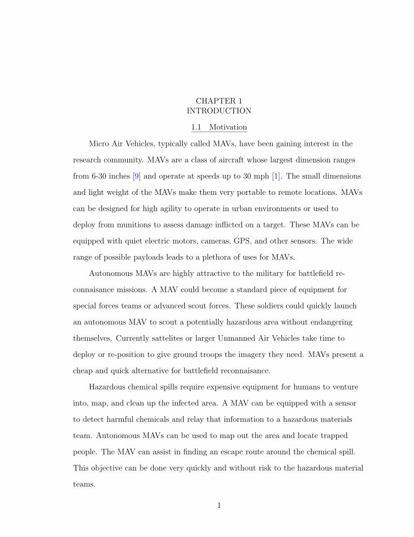
The video signal sent to the ground station is analyzed for pitch percentage
and roll angle. The pitch percentage is the percent of ground seen in the image.
This is calculated by first detecting the horizon by statistical modeling. The
horizon detection algorithm determines the horizon that best divides the image into
”ground” and ”sky” based on previous calibration. The horizon line is also used to
determine the current roll angle. An example of the horizon detection algorithm is
shown in Figure 1–3.
Figure 1–3: Horizon Detection Example
The autopilot consists of a lateral and longitudinal stability augmentation
system, directional controller, and an altitude control system. The lateral stability
augmentation system stabilizes the vehicle and allows tracking of roll commands.
The architecture of the lateral stability augmentation system is shown in Figure
1–4. The controller consists of a integral gain KIφ , porportional gain Kφ, a filter ∆,
a camera C, and a vision processing element V .

7
- ∆ -
-Kφ6
-KIφ?-MAV -
�C�V
?
�
environment
Figure 1–4: Lateral stability augmentation system
The longitudinal stability augmentation system stabilizes the AVCAAF
vehicle and tracks pitch percentage commands. The architecture of the lateral
stability augmentation system is shown in Figure 1–5. The controller consists of a
porportional Kσ, a camera C, and a vision processing element V .
- -Kσ-MAV -
�C�V
?
�
environment
Figure 1–5: Longitudinal stability augmentation system
The directional controller is an outer loop of lateral stability augmentation
system shown in Figure 1–6. Here Kψ is the porportional gain and S is the GPS
sensor. The current longitude and lattitude is provided by the GPS receiver at a
1 Hz rate. The heading is calculated from the current and previous GPS position.
This creates a lag in the system to calculate the heading and does not provide
real-time GPS coordinates. This issue is addressed by calculating position and
heading estimates which update at the 50 Hz rate of the control system.
The altitude controller commands the altitude to reach the correct altitude
of the current waypoint. Included in this controller is a switching element to
use altitude error or pitch percentage error to determine the elevator deflection

8
ψc- -Kψ- ∆ -
-Kφ6
-KIφ?-MAV -
�C�V
?
�
environment
�S
6
Figure 1–6: Directional control system
shown in Figure 1–7. Here KIh is the altitude integral gain, Kh is the altitude
porportional gain, and Kφδeis a gain to couple the longitudinal dynamics with the
lateral-directional dynamics. The controller limits the pitch percentage to ensure
that there is always a visible horizon for pitch percentage and roll angle calculation.
hc--Kh
6
-KIh?-switch- -MAV -
�C�V��Kσ
-
- lim
? �
environment
�S
6
6
Kφδe
6
Figure 1–7: Altitude control system
The AVCAAF autopilot underwent a series of flight tests to experimentally
tune the various gains of the control systems. These flight tests resulted in an
autopilot capable of 3-D waypoint navigation. Figure 1–8 shows the flight path of
the AVCAAF vehicle as it tracks three waypoints, shown in red boxes, multiple
times.
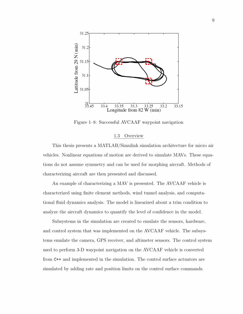
9
Figure 1–8: Successful AVCAAF waypoint navigation
1.3 Overview
This thesis presents a MATLAB/Simulink simulation architecture for micro air
vehicles. Nonlinear equations of motion are derived to simulate MAVs. These equa-
tions do not assume symmetry and can be used for morphing aircraft. Methods of
characterizing aircraft are then presented and discussed.
An example of characterizing a MAV is presented. The AVCAAF vehicle is
characterized using finite element methods, wind tunnel analysis, and computa-
tional fluid dynamics analysis. The model is linearized about a trim condition to
analyze the aircraft dynamics to quantify the level of confidence in the model.
Subsystems in the simulation are created to emulate the sensors, hardware,
and control system that was implemented on the AVCAAF vehicle. The subsys-
tems emulate the camera, GPS receiver, and altimeter sensors. The control system
used to perform 3-D waypoint navigation on the AVCAAF vehicle is converted
from C++ and implemented in the simulation. The control surface actuators are
simulated by adding rate and position limits on the control surface commands.

10
The process of characterizing micro air vehicles in this thesis will be used to
model future micro air vehicles. This thesis attempts to lay the ground work to
allow controller design on future micro air vehicles.

CHAPTER 2SIMULATION ARCHITECTURE
2.1 Simulation Overview
The MAV simulator is a MATLAB/Simulink program that numerically
integrates the nonlinear equations of motion of the system. The simulator consists
of four major subsystems: Controller K, Actuators A, Nonlinear Dynamics Plant
P , and Sensors S as shown in Figure 2–1.
Figure 2–1: Micro Air Vehicle simulation architecture
The structure of the simulation is built as a “top-down” architecture. Each
subsystem is modular and contains more subsystems which are easily reconfigured.
This architecture allows a “plug-and-play” capability allowing the simulation to
simulate different aircraft, controllers, and sensors easily by simply replacing a
subsystem.
2.2 Non-Linear Dynamics Plant
The structure of the Nonlinear Dynamics Plant, depicted in Figure 2–2, does
not change between aircraft platforms. The other subsystems are specifically
designed for the AVCAAF vehicle and are described in Chapter 6.
11

12
Figure 2–2: Nonlinear dynamics plant
The Air Density Look-Up block finds the air density based on current altitude.
The air density is calculated using first-order interpolation between points from the
standard atmosphere table. It interpolates between -200 meters to 1000 meters;
however, a larger range could be covered if more reference points were added. Table
2–1 shows the altitude and air density values used.
Table 2–1: Standard atmosphere air densities
Altitude (m) Air Density (kg/m3)-200 1.2487-100 1.2368
0 1.2250100 1.2133200 1.2071300 1.1901400 1.1786500 1.1673600 1.1560700 1.1448800 1.1337900 1.12261000 1.1117

13
The NL Dynamics subsystem calculates the forces and moments acting on
the aircraft at each time-step. The subsystem’s inputs are the control surface
deflections, aircraft moments of inertia, aircraft geometry, air density, and 12 states
defining the aircraft’s position, orientation, linear velocity and angular velocity.
The subsystem calculates the new linear and angular accelerations due to the
forces and moments acting on the aircraft. This calculation uses the standard 12
equations of motion [31] and polynomial coefficients that characterize the aircraft,
described in Section 3.4. These accelerations along with the previous velocities are
the output of this subsystem.
The Integrator subsystem numerically integrates the velocities and acceler-
ations each time-step of the simulation. A set of initial conditions can be set by
the user to define the initial position, orientation, and velocity of the aircraft. The
integrator uses these initial values to set the states when the simulation begins.
The Angle Limiter subsystem converts the Euler angles to a range between 0
and 360o.
The Body Axis States to Earth Inertial FOR subsystem converts the current
aircraft position, orientation, and velocity into the Earth inertial frame of reference.
These states are then passed to the Sensor module from Figure 2–1 for sensor use.

CHAPTER 3NONLINEAR EQUATIONS OF MOTION
This chapter derives the nonlinear equations of motions used by the Nonlinear
Dynamics Subsystem presented in Section 2.2. The equations of motion describe
the rigid body dynamics and neglect the structural dynamics. MAVs obey the same
equations of motion as any airplane. The following derivation is for the general
airplane as detailed in [13, 31] and expanded to include assymetries.
3.1 Frames of Reference
The MAV moves in an earth-fixed inertial reference frame E defined by the
basis vectors (e1, e2, e3). The vector e3 points in the same direction as gravity.
Vectors e1 and e2 are positioned to make E a right-handed coordinate system. The
earth-fixed reference frame E is shown in Figure 3–1.
Six Degrees Of Freedom (DOF) are necessary to fully describe the MAV’s
position and orientation from a specified point. The first three DOFs define the
distance from the MAV to the fixed-reference frame. The other three DOFs are
Euler angles and define the rotation between the fixed-reference frame and the
MAV body-fixed reference frame.
The body-fixed reference frame B has its origin at the MAV center of gravity
and is defined by the basis vectors(b1, b2, b3
). The vector b1 points toward the
nose of the MAV, vector b2 points toward the left wing, and vector b3 makes
B a right-handed coordinate system. This orientation is the standard aircraft
body-fixed coordinate frame.
3.2 Rotations
A sequence of three rotations can transform a position from one coordinate
system to another. This sequence of rotations is done, in order, through the three
14

15
Figure 3–1: Earth-fixed and body-fixed frames of reference
Euler angles yaw (Ψ), pitch (Θ), and roll (Φ). This sequence is a standard 3-2-1
rotation. When these rotations are performed, two intermediate reference frames
are created with basis vectors (x1, y1, z1) and (x2, y2, z2). The rotations are
performed in the following order:
1. Rotate the E earth-fixed reference frame about e3 through yaw angle Ψ to
reach intermediate frame (x1, y1, z1).
2. Rotate (x1, y1, z1) about y1 through pitch angle Θ to reach intermediate
frame (x2, y2, z2).
3. Rotate (x2, y2, z2) about x2 through roll angle Φ to obtain body-fixed frame
B.
Figure 3–2 shows the sequence of rotations graphicly. The rotation sequence
can also be shown mathematically Equation 3.1.

16
Figure 3–2: Set of rotations through the Euler angles
b1
b2
b3
=
1 0 0
0 CΦ SΦ
0 −SΦ CΦ
CΘ 0 −SΘ
0 1 0
SΘ 0 CΘ
CΨ SΨ 0
−SΨ CΨ 0
0 0 1
e1
e2
e3
=
CΘCΨ CΘSΨ −SΘ
CΨSΦSΘ− CΦSΨ SΦSΘSΨ + CΨCΦ SΦCΘ
CΦSΘCΨ + SΦSΨ CΦSΘSΨ− CΨSΦ CΦCΘ
e1
e2
e3
= E B
e1
e2
e3
(3.1)
Converting a vector from the body-fixed frame B back to the earth-fixed frame
E is done by inverting the matrix E B and multiplying it by the vector.
3.3 Kinematic Equations
The rigid body equations of motion can be derived from Newton’s second law.
∑F =
d
dt(mv) (3.2)∑
M =d
dtH (3.3)

17
F is the force applied to the rigid body and H is the angular momentum
of the rigid body. The vector components of 3.2 can be decoupled into three
components shown in 3.4.
∑F =
d
dt(mv) c+
d
dt(mv) b2 +
d
dt(mv) b3
= Fxb1 + Fyb2 + Fzb3
(3.4)
Fx, Fy, and Fz are the forces along the{
b1, b2, b3
}axes respectively.
The velocity of the center of gravity (CG) of the MAV is Vc. With the
definition of Vc and the rigid body assumption, velocities at other points on the
MAV may be found.
Let r be the position vector from the CG to a differential mass element δm.
The velocity of this mass element is expressed in 3.5.
V = Vc +dr
dt= Vc + EωB × r (3.5)
Here EωB is the angular velocity of B in E defined in 3.6.
EωB = pb1 + qb2 + rb3 (3.6)
Assuming the mass is constant, then the body-fixed accelerations can be found
using 3.7, 3.8, and 3.9
Fx = m (u+ qw − rv) (3.7)
Fy = m (v + ru− pw) (3.8)
Fz = m (w + pv − qu) (3.9)
The angular momentum of the mass element is expressed in 3.10.

18
∑r × vcδm+
∑ [r ×
(EωB × r
)](3.10)
Expanding r into its components yields 3.11.
r = xb1 + yb2 + zb3 (3.11)
H can now be expressed as 3.12.
H =(pb1 + qb2 + rb3
) ∑ (x2 + y2 + z2
)δm
−∑ (
xb1 + yb2 + zb3
)(px+ qy + rz) δm (3.12)
The scalar parts of H are shown in 3.13, 3.14, and 3.15.
Hx = p∑ (
y2 + z2)δm− q
∑xy δm− r
∑xz δm (3.13)
Hy = −p∑
xy δm+ q∑ (
x2 + z2)δm− r
∑yz δm (3.14)
Hz = −p∑
xz δm− q∑
yz δm+ r∑ (
x2 + y2)δm (3.15)
The summations of 3.13 are the moments and products of inertia defined in
3.16, 3.17, 3.18, 3.19, 3.20, and 3.21. The domain of integration for these equations
is the entire aircraft body.

19
Ixx =
∫ ∫ ∫ (y2 + z2
)δm (3.16)
Iyy =
∫ ∫ ∫ (x2 + z2
)δm (3.17)
Izz =
∫ ∫ ∫ (x2 + y2
)δm (3.18)
Ixy =
∫ ∫ ∫xy δm (3.19)
Ixz =
∫ ∫ ∫xz δm (3.20)
Iyz =
∫ ∫ ∫yz δm (3.21)
Using the equations for the moments and products of inertia, the scalar parts
of H become 3.22, 3.23, and 3.24.
Hx = pIxx − qIxy − rIxz (3.22)
Hy = −pIxy + qIyy − rIyz (3.23)
Hz = −pIxz − qIyz + rIzz (3.24)
Using 3.3, 3.22, 3.23, and 3.24 the moment equations can be expressed 3.25,
3.26, and 3.27.
L = Hx + qHz − rHy (3.25)
M = Hy + rHx − pHz (3.26)
N = Hz + pHy − qHx (3.27)
Where L, M , and N are the moments about{
b1, b2, b3
}axes respectively.
Making the assumption that the rate of change of the moments and products of

20
inertia are negligible and assuming the aircraft is not symmetric, the equations can
be expanded into 3.28, 3.29, and 3.30.
L = pIxx − qIxy − rIxz − pqIxz +(r2 − q2
)Iyz + qrIzz + rpIxy − qrIyy (3.28)
M = −pIxy + qIyy − rIyz + rpIxx − qrIxy +(p2 − r2
)Ixz + pqIyz − prIzz (3.29)
N = −pIxz − qIyz + rIzz +(q2 − p2
)Ixy + pqIxy − prIyz − pqIxx + qrIxz (3.30)
Equations 3.7, 3.8, 3.9, 3.28, 3.29, and 3.30 are the equations of motion used in
the simulation.
3.4 Force and Moment Calculations
The forces and moments the aircraft acting on the aircraft are represented
as functions of the flight condition. The flight condition includes angle of attack,
slide-slip angle, aircraft velocity, air density, and control surface deflections. The
equations for the coefficients of the forces and moments are given in 3.31, 3.32,
3.33, 3.34, 3.35, and 3.36.
CL = CLα2α2 + CLαα+ CL0 + CLδsym
δsym + CLαα (3.31)
CD = CDα2α2 + CDαα+ CD0 + CDδsym
δsym (3.32)
CY = CYpp+ CYrr + CYδrδr + CYδasy
δasy + CYββ (3.33)
Cm = Cmα3α3 + Cmα2α
2 + Cmαα+ Cm0 + Cmδsymδsym + Cmα
α (3.34)
Cl = Clpp+ Clrr + Clδrδr + Clδasy
δasy + Clββ (3.35)
Cn = Cnpp+ Cnrr + Cnδrδr + Cnδasy
δasy + Cnββ (3.36)

21
These equations use the methods presented in Chapter 4 to characterize the
aircraft. During each timestep of the simulation, the forces and moments acting on
the aircraft are calculated at that particular instant. This calculation is done by
evaluating 3.31, 3.32, 3.33, 3.34, 3.35, and 3.36 at that particular flight condition.
The coefficients are then multiplied by the current dynamic pressure, wing area,
and reference length if applicable.
3.5 Calculation of States
The body axis linear accelerations are calculated using 3.7, 3.8, and 3.9. The
forces were previously calculated and the mass, current angular rates and velocity
are known.
The body axis angular accelerations are calculated using 3.28, 3.29, and 3.30.
The inertial properties, current angular rates, and moments are known.
These body axis linear and angular accelerations are rotated into the earth-
fixed inertial reference frame and integrated each time step.
CHAPTER 4CHARACTERIZATION METHODS
This chapter presents five different methods that can be used to help charac-
terize aircraft. Some methods may not competely characterize the aircraft so data
from multiple methods can be combined to generate a model.
4.1 Physical Measurements
Physical measurements can be taken directly from the aircraft. Geometric
propetries such as wing span, wing area, and the mean aerodynamic chord can
be approximated using a ruler. The mass is easily obtained using a scale and the
center of gravity can be experimentally located. Torsional pendulums can be used
to determine the moments of inertia and principle axes of the aircraft.
4.2 Finite Element Methods
A high fidelity finite element model can produce analytical values for mass,
moments of inertia, products of inertia, wing area, and other geometric properties.
Programs such as ProEngineer [35] can be utilized to create computer models of
each airplane component. These can then be assembled in a flight configuration.
Subsequent anaylsis can result in values for the aforementioned properties.
4.3 Wind Tunnel
A wind tunnel can be used to accurately characterize forces and moments
acting on a micro air vehicle. Micro air vehicles can be small enough to mount a
full-size MAV model into the wind tunnel test section without requiring scaling
laws. This testing allows the wind tunnel data to include the strong viscous forces
associated with the low Reynolds numbers encountered by MAVs [3].
22

23
Accurate results from wind tunnels depend on the instrumentation used to
measure the forces and moments. A 6 in MAV can have forces on the order of 0.02
newtons [3]. Such small forces can be easily distorted by noise or poor calibration.
Results from wind tunnel testing can include static derivatives and curves for
the forces and moments based on angle of attack, side-slip angle, control surface
deflection, and thrust. Dynamic derivatives can be difficult to measure in a wind
tunnel and is often approximated by equations.
4.4 Computational Fluid Dynamics
The use of Computational Fluid Dynamics (CFD) can assist in evaluating
hard to determine parameters, such as the dynamic derivatives, as well as easier to
determine parameters, such as static derivatives. CFD methods can also be used
when a wind tunnel cannot be used. Vortice Lattice Methods (VLM) can be used;
however, the complete Navier-Stokes equations will provide more accurate results.
Some VLM programs do not include viscid skin friction which becomes a significant
force in low Reynolds number flow.
4.5 Flight Testing
An aircraft equipped with sensors, such as accelerometers and gyroscopes,
can log flight test data for analysis. This data can be used to perform regression
analysis to relate gyro measurements of roll rate, pitch rate, and yaw rate to
control surface commands. The aircraft dynamics are determined by a least-squares
approach to the flight test data [27]. This method can obtain inaccurate results
due to noisy sensor measurements.

CHAPTER 5AVCAAF CHARACTERIZATION
5.1 Overview
This chapter presents an example of characterizing a MAV. This example
consists of identifying the longitudinal and lateral dynamics of the AVCAAF vehi-
cle using finite element methods, wind tunnel and computational data. The wind
tunnel data is used to find the static aerodynamic force and moment coefficients.
The aerodynamic software package, Tornado, approximates the dynamic derivatives
of the AVCAAF vehicle [29]. The aerodynamic characteristics are integrated into
the standard longitudinal and lateral linear dynamics to characterize the AVCAAF
at a trim condition. These linearized dynamics are analyzed for modal properties.
The analysis is performed to check stability and to quantify the confidence of the
model created from the wind tunnel and computational data.
The actual implementation of the dynamics will involve regression analysis
of the wind tunnel data, supplemented by the computational data, resulting in
functions for force and moment coefficients. This implementation allows simulation
of the MAV at different flight conditions.
5.2 Experimental Aerodynamics
5.2.1 Testing
The aerodynamics associated with the AVCAAF aircraft are experimentally
determined using a wind tunnel at the University of Florida. This wind tunnel is a
horizontal, open-circuit low-speed facility. The wind tunnel has a bell mouth inlet
and several flow straighteners. The test section is square with dimensions 914 mm
and a length of 2 m. The fan speed is regulated by a variable frequency controller
24

25
and operated remotely by a computer. The maximum velocity for test purposes is
approximately 15 m/s which correlates to a maximum Reynolds number of 100,000.
Testing of the tunnel is controlled by a computer. This computer controls the
angle of attack of the model along with acquiring data and performing real-time
analysis.
Figure 5–1: AVCAAF model in test section
The vehicle is mounted onto a sting balance and the resulting structure con-
nects to an aluminum arm as in Figure 5–1. The internal sting balance measures
five forces and one moment. The forces are converted in real time to the coeffi-
cients, {CL, CD, Cm, Cn, CY , Cl}, using the dynamic pressure and reference data for
wing area and reference length.
The main potential sources of uncertainty are errors associated with solving
the sting balance forces and moments, angle of attack measurements, and the
dynamic pressure determination. Additional minor factors include uncertainties
in the determination of geometric quantities such as wing area or chord line. In
actuality, the MAV generates loads considerably smaller than usual calibration
weights so the sting balance is a reasonable expectation as the main source
of error [39, 30]. A preliminary estimate of this error was done by running an
extensive set of calibration checks [19].

26
5.2.2 Results
The aerodynamics of the AVCAAF vehicle are determined using a freestream
velocity of 13 m/s . The vehicle was mounted wings-level to consider sweeps across
angle of attack and mounted at a roll angle of 90o to consider sweeps across angle
of sideslip.
A complete set of static derivatives in pitch, roll and yaw are computed [3]. A
representative set of this aerodynamic data is given in Figure 5–2 and Figure 5–3.
These data consider the aerodynamics at a variety of symmetric deflections for the
elevators.
Unfortunately, the facility did not allow for measuring the dynamic deriva-
tives. Consequently, the data obtained from the wind tunnel is not sufficient to
completely characterize a model of the flight dynamics.
The AVCAAF vehicle was also not tested with its motor turned on. Testing
the AVCAAF vehicle with the motor on would require an awkward mouning
system which does not currently exist. Since the differential elevators and rudder
are in the prop-wash during actual flight, the wind tunnel data may not accurately
depict the elevator effectiveness.
−5 0 5 10 15 20−1
−0.5
0
0.5
1
1.5
2
AOA (deg)
CL
δe =0
δe =10
δe =30
Figure 5–2: CL versus angle of attack

27
0 0.05 0.1 0.15 0.2 0.25 0.3 0.35−1
−0.5
0
0.5
1
1.5
2
CD
CL
δe =0
δe =30
Figure 5–3: CL versus CD
5.3 Analytical Inertias
The inertia properties of the aircraft are estimated from finite element
methods. This analysis uses a CAD model, shown in Figure 5–4, and the
ProEngineer [35] software package. The model was created by dimensioning
each component of the MAV and assembling them in a flight configuration. An
exploded view of the ProEngineer model is shown in Figure 5–5 and a list of
components is presented in Table 5.3. The estimated inertia properties are given in
Table 5.3.
Figure 5–4: Analytical model
The model used to calculate these values accounts for the dominant mass
elements; however, some small errors remain. The mass of the model is 6.5% less

28
Figure 5–5: Exploded view
Table 5–1: AVCAAF vehicle component masses
Component Mass (grams)Altimeter Board 27.0
Avionics 61.0Battery 131.7
Camera Mount 5.0Camera Transmitter 18.2
Fuselage 47.9Hatch 6.7
Horizontal Stabilizer 8.9Motor 50.0
Propeller 9.0Propulsion Gearing 24.6
RC Receiver 8.0Servo x3 29.7
Servo Mount 7.0Speed Controller 12.2
Tail Boom 6.5Video Camera 11.9
Vertical Stabilizer 10.6Wing 34.0
Total Mass 509.9
than the actual vehicle because small parts, such as wires and control rods, are
excluded from the model. The center of gravity is also in error and lies 0.125 in aft

29
Table 5–2: Analytical inertia properties
Property kg ·m2
Ixx 1.127 e−03
Iyy 6.604 e−03
Izz 7.130 e−03
Ixy −3.920 e−05
Ixz −3.798 e−04
Iyz −9.670 e−06
of the actual position. These errors are quite small so the properties in Table 5.3
are accepted with reasonable confidence. These values will also be used by the
simulation for the AVCAAF MAV.
5.4 Analytical Aerodynamics
A computational analysis is also used to estimate the aerodynamics of the
vehicle. In this case, the aerodynamics are estimated using the Tornado software
package [29]. This software uses a vortex lattice method to solve for flow over
lifting surfaces. The analysis assumes incompressible flow which is certainly
appropriate for the flight regime of a MAV. The analysis also assumes inviscid flow
which creates some errors in the resulting solution; however, the inviscid pressures
are still represented.
The analysis represents the lifting surfaces as a set of panels. The geometry of
these panels used for the AVCAAF aircraft is shown in Figure 5–6. The software
only considers wings and tails so the fuselage, along with its associated aerody-
namic contribution, is not modeled. The reference point about which moments are
calculated is also shown in Figure 5–6.
A set of static and dynamic derivatives are computed from a central difference
expansion about a given flight condition. In this case, a trim state associated
with straight and level flight is used for the condition. The output contains
almost all of the stability derivatives needed to form a set of full-state linearized

30
0
0.1
0.2
0.3
−0.25−0.2
−0.15−0.1
−0.050
0.050.1
0.150.2
0.25
0
0.05
0.1
Wing x−coordinate
3−D Wing configuration
Wing y−coordinateW
ing
z−co
ordi
nate
Figure 5–6: Geometry of panels
dynamics. Some parameters, such as {CLu , Cmu , CDu}, were neglected because
the aerodynamics were assumed to have no variation with Mach. The dynamic
derivatives obtained from the analysis are listed in Table 5–3.
Table 5–3: Estimated dynamic derivatives
Parameter ValueCmq -6.0391CYp -0.2920CYr 0.7587Cnp 0.0190Cnr -0.3061Clp -0.3857Clr 0.3178
The derivatives in Table 5–3 are accepted with a moderate level of confidence;
however, they are recognized to have some level of error. An obvious source of
error includes the lack of aerodynamic contribution associated with the fuselage.
Another source of error is the effects of a reflexed airfoil which exists on the
physical vehicle but is difficult to model with the software. Tornado also assumes
the lifting surfaces to be rigid. Since the AVCAAF vehicle has flexible wings, the
data obtained from Tornado will not accurately represent the adaptive washout

31
phenomenon. Finally, thrust is not modeled so the analysis assumed thrust equaled
the aligned drag component for the trim condition.
5.5 Model Integration
5.5.1 Wind Tunnel Data Analysis
Regression analysis is used to obtain static derivatives of the force and moment
coefficients from the wind tunnel data. The data was fit to a set of polynomials
representing separate parameters such as lift and pitch moment. Figures 5–7, 5–8,
and 5–9 show the actual wind tunnel data and the curves fitted to the data. The
resulting equations are in radians are 5.1, 5.2, and 5.3.
−4 −2 0 2 4 6 8 10 12−0.6
−0.4
−0.2
0
0.2
0.4
0.6
0.8
1
1.2
1.4
CL
Angle of Attack (deg)
Wind Tunnel DataRegression curve
Figure 5–7: Wind tunnel data and fitted curve of CL
−4 −2 0 2 4 6 8 10 120.02
0.04
0.06
0.08
0.1
0.12
0.14
0.16
0.18
0.2
CD
Angle of Attack (deg)
Wind Tunnel DataRegression curve
Figure 5–8: Wind tunnel data and fitted curve of CD

32
−4 −2 0 2 4 6 8 10 12−0.2
−0.15
−0.1
−0.05
0
0.05
0.1
0.15
Cm
Angle of Attack (deg)
Wind Tunnel DataRegression curve
Figure 5–9: Wind tunnel data and fitted curve of Cm
CD = 5.5475α2 − 1.0587α+ 0.0814 (5.1)
CL = 10.5381α2 + 5.0342α− 0.1514 (5.2)
Cm = −49.2329α3 + 10.7473α2 − 0.8158α− 0.0002 (5.3)
Derivatives of these polynomials were taken with respect to α. Other deriva-
tives that are independent of α were determined by finding a linear relationship
with respect to the associated parameter (β, δr, δsym, etc). Finally, the derivatives
were evaluated at the flight condition used to compute the analytical aerodynamics
corresponding to angle of attack of 5o. This angle of attack is considered a trim
condition and is analyzed only to determine aircraft stability at this condition.
Some anomalies are noted in the experimental aerodynamics. In particular,
the side force shown in Figure 5–10 seems erroneous. The side force during a sweep
through angle of attack should be nearly zero but is measured with a significant
magnitude. The side force during the longitudinal test was actually the same order
of magnitude as that measured during lateral-directional testing that varied rudder
and angle of sideslip. This anomaly is not fully explained but may be caused from

33
the asymmetry of the model, the alignment of the model in the tunnel, or the
calibration of the sting balance.
−4 −2 0 2 4 6 8 10 12−0.06
−0.04
−0.02
0
0.02
0.04
0.06
α (deg)
Cy
Figure 5–10: Measured values of side force
5.5.2 Aerodynamics
The aerodynamics used for analyzing the flight dynamics of the AVCAAF
vehicle are extracted from Table 5–4. These values present both experimental
estimates and analytical estimates. The values in bold font are the actual values
used in formulating the model.
The values extracted from Table 5–4 are divided between the experimental
estimates and analytical estimates. The experimental estimates would normally be
preferred but some anomalies, such as the side force, resulted in higher confidence
being associated with some analytical values. The derivatives with respect to β
were taken from Tornado data due to the wind tunnel data set containing two
values of β at zero and five degrees. The physical mounting of the AVCAAF
aircraft in the wind tunnel currently limits the range of side-slip that can be
measured.
Also, the values of Cmαand CLα
were not obtained from either experimental
analysis or analytical analysis. The value for this parameter was estimated from a
published value for a different vehicle [5].

34
Table 5–4: Analytical and experimental stability derivatives
Stability Derivative Tornado Wind TunnelCLα 4.4486 8.7162Cmα -0.3519 -0.3347CDα 0.4639 -0.2329CYα 0 0.4596CLo 0.5204 -0.2443CDo 0.0166 0.0836Cmo 0.1112 0.0144
CLδsym0.9009 0.7833
Cmδsym-1.6461 -1.4177
CDδsym0.0274 -0.1064
CYδr0.6929 0.1377
Clδr0.0284 0.0753
Cnδr-0.3239 -0.3312
CYδasy0.6859 0.1556
Clδasy-0.0280 -0.0675
Cnδasy-0.2883 -0.2920
CYβ-0.7121 0.4488
Clβ -0.0769 2.2056Cnβ
0.31274 7.6871
The simulation uses the data selected in Table 5–4 as well as the dynamic
derivatives in 5–3 to supplement the wind tunnel data.
5.6 Linearized Dynamics
These modes are initial estimates of the flight dynamics and must be accepted
with caution. The aerodynamics used to generate the model showed discrepancies
between experimental and analytical estimates so the model is inherently question-
able. The aircraft is undergoing flight testing but the sensor package does not yet
measure parameters sufficient for extensive modeling [22].
5.6.1 Longitudinal
The flight dynamics describing longitudinal maneuvers around the trim
condition are computed by combining data from Table 5.3, Table 5–3, and Table 5–
4. The resulting model represents the linearized dynamics for which longitudinal

35
and lateral-directional components are decoupled. The dynamics are realized as a
state-space expression [31].
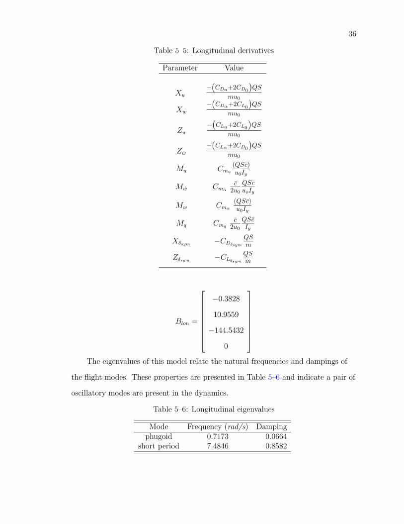
∆u
∆w
∆q
∆θ
= Alon
∆u
∆w
∆q
∆θ
+Blon∆δsym
Where the Alon and Blon matrices are comprised of longitudinal derivatives.
The longitudinal derivatives are defined in Table 5–5.
Alon =
Xu Xw 0 −g
Zu Zw u0 0
Mu +MwZu Mw +MwZw Mq +Mwu0 0
0 0 1 0
Blon =
Xδsym
Zδsym
Mu +MwZδsym
0
The following are the Alon and Blon matrices for the AVCAAF vehicle at
α = 5o.
Alon =
−0.1799 0.4617 0 −9.81
−1.1198 −9.4678 13 0
0.0942 −1.8271 −3.2945 0
0 0 1 0
36
Table 5–5: Longitudinal derivatives
Parameter Value
Xu
−(CDu+2CD0)QS
mu0
Xw
−(CDα+2CL0)QS
mu0
Zu−(CLu+2CL0)QS
mu0
Zw−(CLα+2CD0)QS
mu0
Mu Cmu
(QSc)u0Iy
Mw Cmα
c2u0
QScuoIy
Mw Cmα
(QSc)u0Iy
Mq Cmq
c2u0
QScIy
Xδsym −CDδsym
QSm
Zδsym −CLδsym
QSm
Blon =
−0.3828
10.9559
−144.5432
0
The eigenvalues of this model relate the natural frequencies and dampings of
the flight modes. These properties are presented in Table 5–6 and indicate a pair of
oscillatory modes are present in the dynamics.
Table 5–6: Longitudinal eigenvalues
Mode Frequency (rad/s) Dampingphugoid 0.7173 0.0664
short period 7.4846 0.8582

37
The eigenvectors associated with these eigenvalues are given in polar form in
Table 5–7. Note these are in terms of non-dimensional states.
Table 5–7: Longitudinal eigenvectors
Short Period Mode Phugoid ModeMagnitude Phase Magnitude Phase
∆u 0.1518 −8.22o 1.0264 −102.05o
∆w 1.5590 98.00o 0.0478 −69.12o
∆q 0.0268 149.12o 0.0026 −93.81o
∆θ 1.0000 0.00o 1.0000 0.00o
A mode is described as phugoid mode because of its relationship between
pitch angle and airspeed. The mode has a small natural frequency and is lightly
damped. As such, the mode has characteristics which are classically associated with
a phugoid mode.
The remaining mode is described as a short period mode. This mode has
a close relationship between angle of attack and pitch rate. Also, the natural
frequency of this mode is an order of magnitude higher than the phugoid mode.
Consequently, this mode is similar in nature to the classic definition of a short
period mode.
5.6.2 Lateral-Directional
The flight dynamics associated with lateral-directional maneuvers around
trim are also computed using data from Table 5.3, Table 5–3, and Table 5–4. The
dynamics are again realized as a state-space expression [31].
∆β
∆p
∆r
∆φ
= Alat
∆β
∆p
∆r
∆φ
+Blat
∆δasy
∆δrud

38
Where the Alat and Blat matricies are comprised of lateral directional derivatives,
defined in Table 5–8.
Alat =
Yβ
u0
Yp
u0−
(1− Yr
u0
)g cos θ0
u0
Lβ Lp Lr 0
Nβ Np Nr 0
0 1 0 0
Blat =
0Yδr
u0
Lδasy Lδr
Nδasy Nδr
0 0
The following are the Alat and Blat matrices for the AVCAAF vehicle at
α = 5o.
Alat =
−0.7661 −0.0074 −0.0578 0.7546
−111.8602 −13.1591 10.8419 0
157.6609 0.2247 −3.6182 0
0 1 0 0
Blat =
0 0.7455
−34.0289 109.5044
−147.1914 −166.9433
0 0
The modal parameters are computed from the eigenvalues and eigenvectors
of Alat. The natural frequencies and dampings resulting from the eigenvalues are
given in Table 5–9. In this case, the lateral-directional dynamics have a divergence,
a convergence, and an oscillatory mode.

39
Table 5–8: Lateral directional derivatives
Parameter Value
YβQSCyβ
m
YpQSbCyp
2mu0
YrQSbCyr
2mu0
LβQSbClβ
Ixx
LpQSb2Clp
2Ixxu0
LrQSb2Clr
2Ixxu0
Nβ
QSbCnβ
Izz
Np
QSb2Cnp
2Izzu0
NrQSb2Cnr
2Izzu0
YδrQSCyδr
m
Lδasy
QSbClδasy
Ixx
LδrQSbClδr
Ixx
Nδasy
QSbCnδasy
Izz
Nδr
QSbCnδr
Izz
Table 5–9: Lateral-directional eigenvalues
Mode Frequency (rad/s) Dampingspiral 2.0888 -1.0000
dutch roll 5.7078 0.4526roll 14.4649 1.0000
The eigenvectors associated with the divergence and convergence are given in
Table 5–10. Note these are in terms of non-dimensional states.

40
Table 5–10: Lateral-directional eigenvectors
Roll Mode Spiral ModeMagnitude Phase Magnitude Phase
∆v 0.0045 180o 0.0057 0o
∆p 0.3392 180o 0.0220 0o
∆r 0.0268 0o 0.0490 0o
∆φ 1.0000 0o 0.4502 0o
∆ψ 0.0791 180o 1.0000 0o
The stable mode has obvious characteristics associated with the classical
definition of roll mode. The response of this mode is predominately a roll motion
with only minor variation in angle of sideslip or yaw.
The unstable mode is characterized as a spiral divergence but with some
reservations. The eigenvector indicates the response resembles a classic spiral mode
in that excitation of this mode is essentially yaw with some roll. Conversely, the
magnitude of the eigenvalue is quite large to be considered a spiral pole.
The remaining mode relates to a dutch roll dynamic as evidenced by its
eigenvector in Table 5–11. The motion associated with this mode is a complex
relationship between yaw and roll and angle of sideslip. The phases and magnitudes
slightly differ from the motions of large aircraft; however, the dynamics are clearly
dutch roll.
Table 5–11: Lateral-directional eigenvector
Dutch Roll ModeMagnitude Phase
∆v 0.0160 −117.02o
∆p 0.1338 116.91o
∆r 0.1446 162.61o
∆φ 1.0000 0o
∆ψ 1.0801 45.70o
Also, the natural frequency associated with the dutch roll agrees with a basic
trend. Namely, the magnitude of the natural frequency should increase as wing

41
span decreases. Figure 5–11 indicates the natural frequency estimated for the
AVCAAF aircraft lies along a reasonable curve with values from other aircraft.
10−1
100
101
102
0
5
10
15
20
25
Wingspan (m)
Fre
quen
cy (
rad/
sec)
15 cm Micro Air Vehicle
Black Widow
AVCAAFDragonFly UAV
F−16 Boeing 747
Figure 5–11: Variation in dutch roll frequency
5.7 Modeling Results
This chapter has shown the development of the linearized longitudinal and
lateral dynamics of a micro air vehicle using wind tunnel and computational data.
The wind tunnel data did not include the dynamic derivatives and included some
spurious data. The software package Tornado was used to supplement the wind
tunnel data to complete the model. The linearized model has modal properties that
are similar to standard aircraft modes. The spiral mode was analyzed as unstable.
This instability has not been confirmed by flight testing due to the difficulty of
recognizing spiral divergence during flight. It should be stated again that the
dynamics presented were for one flight condition. The simulation will encompase
a wider range of flight conditions by using functions to solve for the forces and
moments the MAV experiences each time step.
There is not much confidence in this model accurately characterizing the
actual AVCAAF vehicle. This is due to the conflicting results obtained from the
Tornado and wind tunnel data. Some sources of inaccuracies include computational

42
data based on inviscid flow, inaccurate modeling of the flexible wings, difficulty in
modeling the reflexed airfoil, and spurious experimental data.

CHAPTER 6AVCAAF SUBSYSTEMS
The subsystems designed specifically for the AVCAAF aircraft were the
Sensors block, Controller block, and Actuator block in Figure 2–1. This chapter
discusses the design of these subsystems.
6.1 Sensor Subsystem
The Sensors block from Figure 2–1 is comprised of three subsystems for the
AVCAAF vehicle. These subsystems are the Camera, GPS, and Altitude blocks
shown in Figure 6–1.
Figure 6–1: AVCAAF sensors subsystem
6.1.1 Camera Subsystem
The camera subsystem emulates the vision output the controller receives
from the goundstation for horizon analysis. The subsystem calculates the pitch
43

44
percentage seen by the camera based on pitch angle, roll angle, and camera view
angle. Pitch percentage is the percent of “ground” seen in the image. It is assumed
that when the pitch angle and roll angle are zero the pitch percentage is 50%.
This equation can be further modified to account for altitude and distance to the
horizon.
6–2 shows a side view of the MAV capturing an image with its camera. This
case assumes there is no roll angle. Here γ is the camera view half-angle, θ is the
pitch angle, A − A is the image plane, and D is the length from the camera to the
image plane. L is the length from the camera to the image plane along the camera
half-angle γ. hp is the percentage of ground seen in the image plane. The geometric
identities 6.1 and 6.2 can be observed.
Figure 6–2: Image projection and pitch percentage
L =D
cos (γ)(6.1)
hp = L sin (γ)−D tan (θ) (6.2)
6.2 can be expanded into 6.3.
hp = D (tan (γ)− tan (θ)) (6.3)

45
The pitch percentage can be found be dividing hp by the image plane length,
shown in 6.4. The controller for the AVCAAF vehicle requires this value to be
between 0 and 1, where 1 correlates to a pitch percentage of 100% (“ground”
completely fills the image).
pitch % =hp
2D tan (γ)
=D (tan (γ)− tan (θ))
2D tan (γ)
=1
2− tan (θ)
2 tan (γ)
(6.4)
6.4 is only valid for the case where the roll angle is zero. The equation for
pitch percentage is more complex when roll is added. There are two different
general cases to consider when calculating pitch percentage with roll added. These
cases are when the ground area seen by the camera is either a triangle or trapezoid,
as shown in Figure 6–3.
Figure 6–3: Triangular and trapezoidal ground areas
Figure 6–3 also shows the image taken from the camera is not circular. The
camera in the AVCAAF transmits a standard NTSC video signal. This video
format will also make the pitch percentage calculation more complex. The standard
NTSC signal has a ratio of 3:4 for the height and length of the image respectively.
The pitch percentage will now be calculated as the percent of ground in the
rectangular image plane.

46
Figure 6–4 shows a more detailed view of the rectangular image plane. From
Figure 6–2 the distance from the center of the image to the horizon is found to be
D tan (θ). It is known that the circle encompasing the 3:4 rectangle has a diameter
of 2D tan (γ).
Figure 6–4: NTSC camera image
To find the area of the ground in the image plane, let B represent the in-
tersection of the horizon with the rightmost side of the rectangular image. Since
a negative roll will result in the same pitch percentage as a positive roll of the
same magnitude, all negative rolls will be analyzed as positive rolls to simplify the
calculation.
Let C represent the intersection of the horizon and the leftmost side of the
rectangular image. Let A be the point on the horizon closest to the center of the
image. These points are depicted in Figure 6–5.

47
Figure 6–5: NTSC image box and ground intersection
The coordinates of A, B, and C are taken from the center of the image, given
in 6.5, 6.6, and 6.7.
A = (−D tan (θ) sin (φ) ,−D tan (θ) cos (φ)) (6.5)
B = (−D tan (θ) sin (φ) + S cos (φ) ,−D tan (θ) cos (φ)− S sin (φ)) (6.6)
C = (−D tan (θ) sin (φ)− P cos (φ) ,−D tan (θ) cos (φ) + P sin (φ)) (6.7)
The value of P and S will depend on the orientation of the horizon. There
are two cases for the location of point B: point B is either on the rightmost image
boundary or on the bottom image boundary. The camera subsystem assumes that
the roll angle of the AVCAAF vehicle will not exceed ±90o meaning the MAV will
not be inverted. The camera subsystem also converts a negative roll angle into a
positive angle for the pitch percentage calculation; the same magnitude roll angle
will result in the same pitch percentage if it is negative or positive.
To solve for the length S from Figure 6–5, the two cases for the location of
point B are evaluated. Setting the x-coordinate of B to 45D tan (γ) sets B at the

48
rightmost image boundary. Setting the y-coordinate of B to −35D tan (γ) sets B at
the bottom image boundary. The length of S for both cases are 6.8 and 6.9.
S =D
cos (φ)
(4
5tan (γ) + tan (θ) sin (φ)
)Rightmost Boundary (6.8)
S =D
sin (φ)
(3
5tan (γ)− tan (θ) cos (φ)
)Bottom Boundary (6.9)
The correct value for S will be the minimum positive value resulting from 6.8
and 6.9. A similar method is used to find the value of P .
P =D
cos (φ)
(4
5tan (γ)− tan (θ) sin (φ)
)Leftmost Boundary (6.10)
P =D
cos (φ)
(tan (θ) cos (φ)− 3
5tan (γ)
)Bottom Boundary (6.11)
The area of ground seen in the image plane is now simply a combination of
triangle and rectangle areas. Figure 6–6 shows a simulation of the horizon line
based on a 10o pitch angle and a 25o roll angle. The circle indicates the center of
the image. This image is similar to Figure 1–3 depicting an image processed by the
real horizon detection algorithm. Here the lower left corner underneath the line is
considered “ground.”
6.1.2 GPS Subsystem
The GPS subsystem gives the controller the current longitude and lattitude.
Using the equations 6.12 and 6.13, the subsystem determines the current lattitude
and longitude based on the starting position and current position. The actual GPS
receiver on the AVCAAF vehicle refreshes at a 1 Hz rate. This refresh rate has to
be simulated in Simulink to accurately model the GPS receiver.

49
−0.5 −0.4 −0.3 −0.2 −0.1 0 0.1 0.2 0.3 0.4 0.5
−0.4
−0.3
−0.2
−0.1
0
0.1
0.2
0.3
0.4
Figure 6–6: Simulated horizon from camera subsystem
1 Longitude minute = 1582 cos (Lattitude degrees)meters (6.12)
1 Lattitude minute = 1582 meters (6.13)
6.1.3 Altitude Subsystem
The altimeter on the actual AVCAAF aircraft measures pressure and outputs a
signal of 0 - 5 volts. The avionics package of the AVCAAF vehicle takes this signal
and uses a 8-bit A-D converter changing the signal into an integer from 0-255.
For the purposes of simulating this signal, it is assumed the altimeter has a one
meter per integer resolution, based on pilot observation. Thus, a simple calculation
emulates the altimeter: altimeter reading equals initial altimeter reading minus
the earth-fixed inertial frame Z value (a negative Z value corresponds to a positive
altitude).
6.2 Actuator Subsystem
The Actuator subsystem allows saturation and rate limits to be imposed on
the control servos. The position limits are ± 20o on the differential elevators and
± 25o on the rudder. The rate limits are 260 deg/s for all the servos. This actuator
modeling helps make the simulation more realistic.

50
6.3 Controller Subsystem
The Controller subsystem controls the differential elevators and rudder
deflections. Future simulations for morphing aircraft will allow the controller to
change the geometry of the MAV by changing the moments of inertia, products of
inertia, wing area, wing span, and mean aerodynamic chord.
The current contoller implemented in this subsystem was taken from the
AVCAAF vehicle controller. The original controller was coded in C++ and converted
into a MATLAB/Simulink implementation manually. This controller has the ability
to perform three dimensional waypoint navigation. The waypoints are pre-defined
by the user. The controller gives control surface commands to the MAV to reach
the waypoints. This controller can only change the differential elevator deflections.
In the actual AVCAAF control system the ground station sends symmetric and
anti-symmetric elevator commands to the Radio Control (RC) transmitter. The RC
transmitter mixes these signals to create individual control surface deflections. The
RC transmitter was programmed to use 100% of the symmetric elevator deflection
command and 75% of the anti-symmetric deflection command when computing the
servo commands. This signal mixing was implemented in the controller subsystem.
CHAPTER 7RESULTS AND CONCLUSIONS
7.1 Results
The example MAV characterized in Chapter 5 and 6 was not successfully
simulated. The attempt at simulating the AVCAAF vehicle resulted in an unstable
aircraft that could not be controlled by the Controller subsystem. The gains were
adjusted by a trial and error method but failed to control the aircraft. This failure
to accurately simulate the AVCAAF vehicle and control system was mainly due
to the modeled AVCAAF vehicle not accurately representing the actual AVCAAF
vehicle.
7.2 Conclusion
This thesis has developed a simulation environment for Micro Air Vehicles
(MAVs). This simulation was designed to have a “plug-and-play” capability with
the aircraft sensors, aircraft, and controllers to make it easy for the user to simulate
various aircraft using different control systems.
A set of nonlinear equations of motion were derived for asymmetric aircraft.
These equations require characterization of the forces and moments encountered by
the MAV. The controller subsystem can utilize the asymmetric equations of motion
to control morphing aircraft by changing the aircraft geometry
An example MAV characterization is presented in this thesis. The AVCAAF
vehicle, a 24 in wingspan MAV, was modeled using physical measurements, finite
element methods, wind tunnel testing, and computational fluid dynamics analysis.
The subsystems representing the AVCAAF vehicle’s sensors and control system
were developed to emulate the actual hardware and software. The result of the
AVCAAF vehicle modeling did not result in an accurate simulation. The control
51

52
system implemented in the simulation had the same architecture and gains as used
on the actual AVCAAF vehicle. Since the dynamics differ between the actual and
modeled AVCAAF vehicle, it is not surprising that the control system could not
control the simulated vehicle.
The ground work for simulating MAVs has been established. Methods to
characterize MAVs have been attempted. Further research will more accurately
model MAVs. Accurate characterization will allow the simulated vehicle to
accurately represent the actual vehicle making controller design possible in the
simulated environment.

CHAPTER 8RECCOMENDATIONS
8.1 Overview
This chapter is intended to present reccomendations for the AVCAAF pro-
gram.
8.2 Wind Tunnel Characterization
Using the wind tunnel to characterize MAVs is ideal. The wind tunnel
allows accurate characterization of actual flight conditions using the actual MAV.
Refinement in characterizing the Micro Air Vehicles needs to be researched.
Problems associated with testing the AVCAAF vehicle included:
• Limited angle of attack range
• Unreliable side force component
• Limited side-slip angle range
• Testing did not include powered thrust
• Dynamic derivatives could not be obtained
Testing the second generation AVCAAF vehicle (denoted as AVCAAF
vehicle 2.0) has recently started. The configuration of the new vehicle eliminates
some of these problems. The AVCAAF vehicle 2.0 has been tested through a
complete range of angle of attack including stall angle. The testing has also
included powered thrust since the wind tunnel mounting does not interfere with the
propeller.
Despite the AVCAAF vehicle 2.0 improvements the side force and dynamic
derivatives are still lacking. Refinement in the side force component must be
accomplished to provide accurate results. The dynamic derivatives may prove to
53

54
be impractical to measure in the wind tunnel and should be the only parameters
approximated by computer.
8.3 Computational Fluid Dynamics Characterization
There are two major problems with using computational fluid dynamics to
characterize the MAVs: poor MAV geometry representation and lack of viscous
forces. The current CFD program, Tornado, did not include the MAV fuselage,
flexibility of the wings, and did not model the reflexed wing curvature.
Fluent, another CFD program, is reccomended to replace Tornado. Fluent
has the capability of importing Computer Aided Drafting models from programs
such as NASTRAN to accurately model the entire MAV. This will allow the flex-
ibile wings to be represented and analyzed accurately as they deform through
flight. Fluent also includes viscous forces that MAVs will encounter at their low
Reynold’s number flight regimes. These capabilities of Fluent should result in
accurate approximations of the dynamic derivatives.
8.4 Streamlining MAV Design to CFD Characterization Process
Currently MAV fuselages are hand made from hard foam to make molds. This
process introduces asymmetries in the fuselage and makes it difficult to create an
accurate computer model of the fuselage. It is reccommended that the design of the
fuselages should be created in a CAD program compatible with Fluent. This will
allow the designer to eliminate fueslage asymmetries and will streamline the process
from design to CFD characterization. The CAD model will be easy to import into
Fluent and be accurately analyzed.
8.5 Miscellaneous Reccomendations
Since the two graduate students working on modeling MAVs are graduating
in Decemeber 2004, this will result a loss of knowledge unless someone is trained
in this area. At least one graduate student should be commisioned to become
familiar with the work presented in this thesis. This should include familiarization

55
in testing proceedures and simulation architecture and code. The student should
also start dialogue with the person in charge of the HILS facility to determine how
to implement the simulation in the facility.

REFERENCES
[1] M. Abdulrahim, H. Garcia, R. Lind, “Flight Testing a Micro Air VehicleUsing Morphing for Aeroservoelastic Control,” AIAA Structures, StructuralDynamics, and Materials Conference, Palm Springs, CA, AIAA-2004-1674,April 2004.
[2] American Institute of Aeronautics and Astronautics, “Calibration and Useof Internal Strain Gage Balances with Application to Wind Tunnel Testing,”Recommended Practice AIAA R-091-2003.
[3] R. Albertani, P. Hubner, P. Ifju, R. Lind, J. Jackowski, “ExperimentalAerodynamics of Micro Air Vehicles,” submitted to SAE World AviationConference, Reno, Nevada, November 2004.
[4] M. Amprikidis and J.E. Cooper, “Development of Smart Spars for ActiveAeroelastic Structures,” AIAA-2003-1799, 2003.
[5] J.H. Blakelock, Automatic Control of Aircraft and Missiles, John Wiley &Sons, Inc., New York, NY, 1965.
[6] J. Blondeau, J. Richeson and D.J. Pines, “Design, Development and Testingof a Morphing Aspect Ratio Wing using an Inflatable Telescopic Spar,”AIAA-2003-1718.
[7] J. Bowman, B. Sanders and T. Weisshar, “Evaluating the Impact of MorphingTechnologies on Aircraft Performance,” AIAA-2002-1631, 2002.
[8] D. Cadogan, T. Smith, R. Lee and S. Scarborough, “Inflatable and RigidizableWing Components for Unmanned Aerial Vehicles,” AIAA-2003-1801, 2003.
[9] R. Causey “A Lateral Vision-Based Control Autopilot For Micro Air VehcilesUsing a Horizon Detection Approach,” Master of Science Thesis 2003.
[10] C.E.S. Cesnik and E.L. Brown, “Active Warping Control of a Joined-WingAirplane Configuration,” AIAA-2003-1716, 2003.
[11] J.B. Davidson, P. Chwalowski and B.S. Lazos, “Flight Dynamic SimulationAssessment of a Morphable Hyper-Elliptic Cambered Span Winged Configura-tion,” AIAA-2003-5301, 2002.
[12] M. Drela, “Higher-Order Boundary Layer Formulation and Application toLow Reynolds Number Flows,” in Fixed and Flapping Wing Aerodynamics for
56

57
Micro Air Vehicle Applications, edited by T.J. Mueller, American Institute ofAeronautics and Astronautics, Reston VA, 2001.
[13] B. Etkin and L.D. Reid, Dynamics of Flight, John Wiley and Sons, Inc., NewYork, NY, 1996.
[14] S.M. Ettinger, M.C. Nechyba, P.G. Ifju and M. Waszak, “Vision-Guided FlightStability and Control for Micro Air Vehicles,” IEEE International Conferenceon Intelligent Robots and Systems, October 2002, pp. 2134-2140.
[15] H. Garcia, M. Abdulrahim and R. Lind, “Roll Control for a Micro Air Vehicleusing Active Wing Morphing,” AIAA Guidance, Navigation and ControlConference, AIAA-2003-5347, 2003.
[16] J.M. Grasmeyer and M.T. Keennon, “Development of the Black Widow MicroAir Vehicle,” AIAA-2001-0127, 2001.
[17] P.G. Ifju, D.A. Jenkins, S. Ettinger, Y. Lian, W. Shyy and M.R. Waszak,“Flexible-Wing-Based Micro Air Vehicles,” AIAA-2002-0705, 2002.
[18] J. S. Jangy and C. J. Tomlinz, “Longitudinal Stability Augmentation SystemDesign for the DragonFly UAV Using a Single GPS Receiver,” AIAA-2003-5592, 2003.
[19] J. J. Jackowski, K. Boothe, R. Albertani, R. Lind, and P. G. Ifju, “Modelingthe Flight Dynamics of a Micro Air Vehicle,” submitted to European MicroAir Vehicle Conf., July 2004.
[20] C.O. Johnston, D.A. Neal, L.D. Wiggins, H.H. Robertshaw, W.H. Mason andD.J. Inman, “A Model to Compare the Flight Control Energy Requirements ofMorphing and Conventionally Actuated Wings,” AIAA-2003-1716, 2003.
[21] S. Jung, ”Design and Development of a Micro Air Vehicle (MAV): Test-Bed forVision-Based Control,” Master of Science Thesis 2004.
[22] J. Kehoe, J. Grzywna, R. Causey, J. Plew, M. Abdulrahim, M. Nechyba andR. Lind, “Waypoint Navigation for a Micro Air Vehicle using Vision-BasedAttitude Estimation,” European Micro Air Vehicle Conference, July 2004.
[23] P.J. Kunz and I. Kroo, “Analysis and Design of Airfoils for Use at Ultra-lowReynolds Numbers,” in Fixed and Flapping Wing Aerodynamics for MicroAir Vehicle Applications, edited by T.J. Mueller, American Institute ofAeronautics and Astronautics, Reston VA, 2001.
[24] E.V. Laitone, “Wind Tunnel Tests of Wings and Rings at Low ReynoldsNumbers,” in Fixed and Flapping Wing Aerodynamics for Micro Air VehicleApplications, edited by T.J. Mueller, American Institute of Aeronautics andAstronautics, Reston VA, 2001.

58
[25] Y. Lian and W. Shyy, “Three-Dimensional Fluid-Structure Interactions of aMembrane Wing for Micro Air Vehicle Applications,” AIAA-2003-1726, April2003.
[26] L. Ljung, System Identification, Prentice Hall, Englewood Cliffs, NJ, 1987.
[27] R. Maine and K. Iliff, ”Application of Parameter Estimation to AircraftStability and Control,” NASA Reference Publication 1168, June 1986.
[28] P. de Marmier and N. Wereley, “Morphing Wings of a Small Scale UAV UsingInflatable Actuators for Sweep Control,” AIAA-2003-1802, 2003.
[29] T. Melin, “A Vortex Lattice MATLAB Implementation for Linear Aero-dynamic Wing Applications,” Master of Science Thesis, Royal Institute ofTechnology(KTH), 2000.
[30] T.J. Mueller, “ Aerodynamic Measurements at Low Reynolds Numbers forFixed Wings MAVs,” RTO/VKI Special Course, VKI, Rhode Saint Gense,Belgium 1999.
[31] C.R. Nelson, Flight Stability and Automatic Control, McGraw-Hill, Inc.,Boston, MA, 1998.
[32] E.W. Pendleton, D. Bessette, P.B. Field, G.D. Miller and K.E. Griffin, “ActiveAeroelastic Wing Flight Research Program: Technical Program and ModelAnalytical Development,” Journal of Aircraft, Vol. 37, No. 4, 2000, pp. 554-561.
[33] B. Sanders, F.E. Eastep and E. Forster, “Aerodynamic and AeroelasticCharacteristics of Wings with Conformal Control Surfaces for MorphingAircraft,” Journal of Aircraft, Vol. 40, No. 1, January-February 2003, pp. 94-99.
[34] W. Shyy, M. Berg and D. Ljungqvist, “Flapping and Flexible Wings forBiological and Micro Air Vehicles,” Progress in Aerospace Sciences, Vol. 35,No. 5, 1999, pp. 455-506.
[35] S. G. Smith, Pro/ENGINEER Wildfire Update Manual, CADquest, Inc.,Harrisburg, PA, 2000.
[36] B.L. Stevens and F.L. Lewis, Aircraft Control and Simulation, John Wiley andSons, Inc., New York, NY, 1992.
[37] G.E. Torres and T.J. Mueller, “Aerodynamic Characteristics of Low AspectRatio Wings at Low Reynolds Numbers,” in Fixed and Flapping WingAerodynamics for Micro Air Vehicle Applications, edited by T.J. Mueller,American Institute of Aeronautics and Astronautics, Reston VA, 2001.

59
[38] D. Viieru, Y. Lian, W. Shyy and P. Ifju, “Investigation of Tip Vortex onAerodynamic Performance of a Micro Air Vehicle,” AIAA-2003-3597, 2003.
[39] M.R. Waszak, L.N. Jenkins and P. Ifju, “Stability and Control Properties of anAeroelastic Fixed Wing Micro Aerial Vehicle,” AIAA-2001-4005, 2001.
[40] M.R. Waszak, J.B. Davidson, and P.G. Ifju, “Simulation and Flight Control ofan Aeroelastic Fixed Wing Micro Aerial Vehicle,” AIAA-2002-4875, 2002.
[41] R.W. Wlezien, G.C. Horner, A.R. McGowan, S.L. Padula, M.A. Scott, R.J.Silcox and J.O. Simpson, “The Aircraft Morphing Program,” AIAA-98-1927,1998.
[42] B. Zhang, Y. Lian and W. Shyy, “Proper Orthogonal Decomposition forThree-Dimensional Membrane Wing Aerodynamics,” AIAA-2003-3917, June2003.

BIOGRAPHICAL SKETCH
Jason Joesph Jackowski was born in Toledo, Ohio, on October 12, 1979.
He grew up in Deltona, Florida, after his family moved when he was three. His
family took an active roll in the Boy Scouts of America and both his brother Jeff
and Jason earned their Eagle Scout awards. Jason persued many extracurricular
activities in high school including acting, KEY club, Academic Team, Environthon
Team, and wrestling. After completing several advanced placement courses in high
school Jason was prepared to attend the University of Florida. Jason completed
his Bachelor of Science degree in Aerospace Engineering. During his undergraduate
degree Jason interned at General Electric Aircraft Engines for one summer and
Boeing for two summers. Jason then decided to attend graduate school at the
University of Florida working in the Flight Controls Laboratory under Dr. Rick
Lind.
60