nonlinear stability of mixed convection flow under non … · nonlinear stability of mixed...

J. Fluid Mech. (1999), vol. 398, pp. 61–85. Printed in the United Kingdom

c© 1999 Cambridge University Press

61

Nonlinear stability of mixed convection flowunder non-Boussinesq conditions.Part 1. Analysis and bifurcations

By S. A. S U S L O V† AND S. P A O L U C C IDepartment of Aerospace and Mechanical Engineering, University of Notre Dame,

Notre Dame, IN 46556, USA

(Received 10 January 1998 and in revised form 26 May 1999)

The weakly nonlinear theory for modelling flows away from the bifurcation point de-veloped by the authors in their previous work (Suslov & Paolucci 1997) is generalizedfor flows of variable-density fluids in open systems. It is shown that special treatmentof the continuity equation is necessary to perform the analysis of such flows andto account for the potential total fluid mass variation in the domain. The stabilityanalysis of non-Boussinesq mixed convection flow of air in a vertical channel is thenperformed for a wide range of temperature differences between the walls, and Grashofand Reynolds numbers. A cubic Landau equation, which governs the evolution ofa disturbance amplitude, is derived and used to identify regions of subcritical andsupercritical bifurcations to periodic flows. Equilibrium disturbance amplitudes arecomputed for regions of supercritical bifurcations.

1. IntroductionThe mixed convection flows considered in this paper typically exist in such tech-

nical applications as chemical vapour deposition reactors, heat exchangers, thermalinsulation systems and others. In many of these applications, the characteristic tem-perature difference is comparable with the average temperature of the fluid and thetemperature gradients are sufficiently large to cause essential fluid property varia-tions (Chenoweth & Paolucci 1985, 1986; Suslov & Paolucci 1995b) which cannot beneglected. Quantitative predictions of flow characteristics such as heat transfer rateor mass flux through these systems is a non-trivial task (Suslov & Paolucci 1995a, b,1997). Indeed, when the properties of a fluid are allowed to vary with temperature andpressure, the momentum and energy equations, which are used to describe the flowof the fluid, become substantially more complicated due to additional nonlinearitiesarising from density, viscosity, thermal conductivity and specific heat variations. Theproperty variations lead to the appearance of additional governing parameters in theproblem. Thus the cost of direct numerical simulations of such flows for all regimesof interest is prohibitively increased. For this reason we have undertaken to studythe character of such flows as a function of the important dimensionless parametersusing weakly nonlinear analysis.

In our earlier works (Suslov & Paolucci 1995a, b) we successfully used the low-Mach-number approximation of the Navier–Stokes equations, instead of the Boussi-

† Current Address: Department of Mathematics and Computing, University of Southern Queens-land, Toowoomba, Queensland 4350, Australia.

62 S. A. Suslov and S. Paolucci

nesq model, to account for the fluid properties variations and analyse the linearstability of the conduction state in a vertical cavity and open channel. It was shownthat the stability characteristics such as the critical Grashof number and the distur-bance wave speed depend strongly on the temperature difference when fluid propertiesare allowed to vary. Moreover, the large density variations, caused by a large tem-perature difference between the walls, can lead to the appearance of a new buoyantinstability which competes with the shear-driven one predicted by the linear analysisof Boussinesq flows.

Linear theory is a universal and powerful technique used to find the locationof bifurcations in parameter space, as well as to predict the form of developingdisturbances. Unfortunately, one cannot obtain the amplitudes of such disturbancesusing linear theory and, consequently, provide any quantitative information about adisturbed flow. Thus, it is necessary to consider nonlinearities in order to close theproblem. Weakly nonlinear theories developed to date (Stuart 1960; Watson 1960;Stewartson & Stuart 1971), and their modifications (Reynolds & Potter 1967; Sen &Venkateswarlu 1983), have been shown to be very powerful tools for the analysis ofstability of various flows. The term ‘weakly’ is used in the application of nonlineartheories to emphasize that such theories use certain expansion procedures and requirethe presence of some ‘small parameter’, the powers of which are used to constructrecursively systems of relatively simple (linear) equations whose solutions constitutethe terms of asymptotic series. These time-dependent series, if convergent, representdeveloping disturbances superposed on the primary flow. The choice of a smallexpansion parameter varies from one approach to another: linear amplification rate,relative distance from the marginal stability surface in the governing parameter space,and the disturbance amplitude itself. Although in the vicinity of a bifurcation point allthese approaches lead to similar results, the ranges of convergence of the asymptoticseries (and of validity of the analysis) depend strongly on the choice of the expansion(Yao & Rogers 1992). Moreover, the relative distance from the neutral stability curvecannot be used as a small parameter when linear analysis shows that the basic flowis always stable and no neutral surface exists, such as in plane Couette or pipePoiseuille flows. The same restriction applies when the linear amplification rate isassumed small, since this would be so only close to the marginal stability surface. Themost natural and general approach seems to be when expansions are made based ona small disturbance amplitude assumption. Since disturbance amplitudes can possiblyremain small for relatively large distances from the bifurcation point, such a techniquecould potentially remain valid for larger parameter ranges and it can be applied evento flows for which marginal surfaces do not exist (Davey & Nguyen 1971). Thevalidity of the small-amplitude assumption has to be checked a posteriori whennonlinear equilibrium states are formally computed. The application of an amplitudeexpansion (Watson 1960) is typically done in conjunction with a multiple-timescaletechnique where the fast timescale corresponds to the exponential disturbance timedevelopment as predicted by linear analysis. Slower timescales correspond to stageswhen the growth or decay of the disturbances is influenced by nonlinearities ofdifferent orders. Frequently, it is argued that the introduction of multiple timescalesis reasonable only when linear disturbances change slowly with time, i.e. when theirlinear amplification or decay rates are small, since in this case the linear developmentstage is sufficiently long. We should note here that the length of the linear stageis not a factor defining the validity of the introduction of multiple timescales. Themultiple-timescale approach is valid no matter how large the linear amplification rateis, provided that the amplitude dynamics changes substantially as the disturbance

Nonlinear stability of mixed convection flow. Part 1 63

develops. This is always the case if an equilibrium state exists. Then the fast timescalecorresponds to the amplitude dynamics away from saturation, while slow scales areintroduced for nearly equilibrium regimes.

After amplitude and multiple-timescale expansions are made, separation of dif-ferent orders in amplitude leads to successive sets of linear equations. An integralsolvability condition must be satisfied in order to find a solution close to the marginalstability surface (Stewartson & Stuart 1971; Stuart 1960; Watson 1960). This ap-proach is used to find the value of the constant entering the Landau equation whichdescribes the time-dependent behaviour of the disturbance amplitude. The value ofthe Landau constant typically is found using appropriate integrals of the eigenfunc-tions computed at the critical point. This automatically limits the applicability ofnonlinear theories to a close vicinity of the bifurcation point. On other hand theeigenfunctions of the linearized problem and their integrals can be computed at anarbitrary point in parameter space regardless of the actual location of the criticality.This suggests using them to determine the Landau constant for an arbitrary set ofgoverning parameters. Unfortunately, this approach faces an inherent difficulty. Aswas first noted by Herbert (1983), the equations at third order in amplitude becomeunconditionally solvable when the linear amplification rate is not equal to zero. Thusthe application of a solvability condition for the evaluation of the Landau constantbecomes meaningless. In order to avoid this difficulty in determining the Landauconstant, Herbert proposed fixing the disturbance at some particular spatial pointsuch that it is determined completely by the eigenfunction of the linear problem. Wehave shown in Suslov & Paolucci (1997) that this procedure leads to an inconsistencyin the definition of the equilibrium disturbance amplitude and, subsequently, we haveproposed replacing the solvability condition with an appropriate orthogonality condi-tion when analysing supercritical or subcritical flows. The idea of orthogonalizing thesolutions of successive systems of equations resulting from weakly nonlinear analysiscan be found in Sen & Venkateswarlu (1983), but in Suslov & Paolucci (1997) it wasshown rigorously that it is not only desirable, but also necessary. Thus the theory wedeveloped in Suslov & Paolucci (1997) does not require amplitude expansions to bebased on the eigenfunctions of the linearized problem computed at the critical point,but rather at a particular point of interest in the parameter space. Consequently, atypical limitation of weakly nonlinear theories to the relatively small neighbourhoodof the bifurcation point is relaxed such that, presumably, our approach remains validfor larger distances from criticality.

There are two major differences between Boussinesq and non-Boussinesq flows inthe light of the weakly nonlinear analysis. First, in the Boussinesq limit, where fluidproperties are assumed to be constant, the governing equations have a quadraticnonlinearity. However, in non-Boussinesq regimes the nonlinear character of theequations is largely governed by the form of the constitutive equations for the fluid,and in general it is not even of polynomial character. This is the case, for example,when the well-known Sutherland formulae are used to describe viscosity and thermalconductivity variations with temperature. Recently, the present authors extended theapplication of Watson’s (1960) theory to the stability of the flow of a general fluid(Suslov & Paolucci 1997). The form of the expansion was rigorously derived based onTaylor expansions of properties about the reference distributions. This enabled us toexamine successfully the stability of non-Boussinesq natural convection in a verticalcavity subjected to large temperature differences (Suslov & Paolucci 1997) and topredict mean flow characteristics and disturbance amplitudes at substantial distancesfrom the critical points.


Second, in contrast to the Boussinesq case, under non-Boussinesq conditions thedensity of the fluid can change with time. This means that in general the total mass ofthe fluid in an open system changes. Such a situation requires a special treatment inthe weakly nonlinear analysis, which to the authors’ knowledge has not been discussedproperly in the literature to date. In the present paper an important modificationof the continuity equation valid for low-Mach-number flows is proposed in order toextend our previously derived theory to flows in open geometries. In this case thetotal mass of the fluid can vary because of disturbance development. This total masschange affects the mean flow of the fluid and, consequently, the average characteristicsof the flow which are of primary interest to engineers.

The amplitude expansion method has been used successfully for supercritical flows.Severe difficulties arise though in applying it in subcritical regimes where the linearamplification rate is negative. Mathematically it becomes impossible to solve thesystem of linear equations at certain points in wavenumber space. These pointscorrespond to so-called mean flow resonances. Physically this means that there is astrong interaction between the mean flow variation induced by the finite-amplitudeperiodic disturbance and the time-dependent mean flow itself. The more subcriticalthe flow is, the more resonance points exist (Davey & Nguyen 1971). Reynolds &Potter (1967), to get around this difficulty, proposed considering the ‘false problem’for subcritical flows where the time evolution of disturbances is neglected and onlysteady equilibrium amplitudes are sought (assuming they exist). Mathematically thisapproach does not lead to any difficulties when, for example, threshold amplitudesfor the subcritical plane Poiseuille flow are estimated. On other hand, the valuespredicted are in poor agreement with experimental results (e.g. by Nishioka, Iida &Ichikawa 1975). One of the reasons for the disagreement could be that this proposedmathematically simple approach does not account for important physical mechanismswhich are present in real flows. Thus, in the present work, the authors prefer to use the‘true problem’ approach where complete amplitude dynamics is considered. However,in treating subcritical regimes, we stay away from the resonant points where thepresent single mode analysis is not adequate. We note that the effects of resonancescould be analysed by using a system of the coupled Landau equations, but this isbeyond the scope of the present work.

Finally, we note that in Suslov & Paolucci (1995b) we carried out a linear stabilityanalysis of non-Boussinesq mixed convection flow in a vertical channel and determinedthe bifurcation points, where transitions from parallel shear flows to periodic flowsoccur, for a complete range of governing parameters. A number of physically distinctinstabilities not found in Boussinesq flows, as well as codimension-2 points, whereinstability modes compete with each other, were identified. In the first part of thepresent paper we augment the previous findings with the analysis of bifurcations andquantitative estimations of equilibrium disturbance amplitudes in post-bifurcationstates while in the second part (Suslov & Paolucci 1999) we discuss mean flowdistributions and energetics corresponding to different modes of instability.

This part of the paper is organized as follows. First, the problem is formulated fortwo physically distinct cases: fixed average longitudinal pressure gradient and fixedaverage mass flux through the channel. Next, the expansion procedure is outlinedand properties of the resulting system of equations are discussed. Special attention ispaid to the treatment of the mean flow in a system with variable total mass. Finally,the theory is applied to the non-Boussinesq mixed convection flow of air in a verticalchannel. Results are given for a wide range of Grashof and Reynolds numbers, andtemperature differences between the walls.


2. Problem definition and governing equationsWe consider a two-dimensional mixed convection flow between two vertical infinite

plates separated by a distance H . We limit ourselves to two-dimensional flows sincelinear stability analysis (Suslov & Paolucci 1995b) shows that the mixed convectionflow becomes first unstable with respect to two-dimensional disturbances. The platesare isothermal and maintained at the different temperatures T ∗h and T ∗c (<T ∗h ) respec-tively (asterisks denote dimensional quantities). The channel is placed into a uniformvertical gravitational field g. Since we are interested primarily in the case of largetemperature differences ∆T = T ∗h − T ∗c , the conventional Boussinesq approximationis not applicable and we adopt the low-Mach-number approximation (Paolucci 1982)for the Navier–Stokes equations in order to describe such a flow:

∂

∂t(ρui) +

∂

∂xj(ρuiuj) = −∂Π

∂xi+Gr

2ε(ρ− 1)ni +

∂τij

∂xj, (1)

ρcp

(∂T

∂t+ uj

∂T

∂xj

)=

1

Pr

∂

∂xj

(k∂T

∂xj

), (2)

∂ρ

∂t+∂ρuj

∂xj= 0, (3)

where

τij = µ

[(∂ui

∂xj+∂uj

∂xi

)− 2

3δij∂uk

∂xk

]. (4)

Here ui = (u, v) and xi = (x, y) are velocity components and coordinates in thehorizontal and vertical directions respectively, and ni = (0,−1) is a unit vector in thedirection of gravity. The boundary conditions for the problem are

u = v = 0 and T = 1 ± ε at x = 0, 1. (5)

The above system is complemented by the equation of state and property variations

ρ = ρ(T ), cp = cp(T ), µ = µ(T ), k = k(T ), (6)

where ρ is the fluid density, µ is the dynamic viscosity, k is the thermal conductivity,and cp is the specific heat at constant pressure, all dependent on the local temperatureT . The equations are non-dimensionalized by the use of channel width H , referencetemperature Tr = (T ∗h + T ∗c )/2, and viscous speed ur = µr/(ρrH). All propertiesof the fluid are made dimensionless using their respective values at the referencetemperature. Note that since we assume that the channel is open to the atmosphere,the total mass of the fluid in the channel in general can change with time. The inlet–outlet conditions for the problem can be of two types: fixed average longitudinalpressure gradient or fixed average mass flux through the channel. Let us assume thataway from the ends the flow is periodic in the longitudinal direction with wavelengthλ. Then, the dynamic pressure gradient averaged over the cross-section is

∂Π

∂y=

∫ 1

0

∂Π

∂ydx =

∂

∂y

(∫ 1

0

Π dx

)=∂Π

∂y, (7)

where the overbar denotes integration over the channel width. Averaging over thewavelength in the longitudinal direction gives

1

λ

∫ y0+λ/2

y0−λ/2∂Π

∂ydy ≡ Π = const. (8)


for the constant average pressure gradient case. Consequently, we can write

Π(x, y) = (const + Πy) +Π ′(x, y), (9)

where Π ′ is periodic in the y-direction. For the case of constant mass flux, condition(8) is replaced by

1

λ

∫ y0+λ/2

y0−λ/2ρv dy ≡ m = const. (10)

The first of these two conditions generally leads to an unknown mass flux through thechannel when the disturbances modify the primary flow, while the second conditionleads to a variation of an unknown average vertical pressure gradient Π associatedwith the development of the secondary flow. The latter situation is somewhat similarto the flow in a closed cavity where in that case m ≡ 0 (see Suslov & Paolucci 1997),although in the open channel the mass flux generally is not zero for non-Boussinesqconditions.

The dimensionless parameters appearing in the equations are respectively theGrashof number, the temperature difference, and the Prandtl number:

Gr =ρ2r βrg∆TH3

µ2r

, ε =1

2βr∆T , P r =

µrcpr

kr, (11)

where βr is the coefficient of thermal expansion evaluated at the reference temperature.Another dimensionless parameter entering the system through the inflow–outflowboundary conditions is the Reynolds number

Re =ρrUrH

µr. (12)

It is associated with the characteristic longitudinal velocity

Ur = − H2

12µrΠ∗, (13)

induced by the imposed pressure gradient Π∗ when the constant pressure gradientcase is considered. Alternatively the characteristic speed is given by

Ur =m∗

ρrH− ρ∗v∗

ρrH, (14)

when the mass flux is fixed. Definitions (13) and (14) result in identical values onlyin the Boussinesq limit when the fluid density is constant. Thus, in non-Boussinesqregimes when the fluid density varies across the channel the two definitions of Ur

lead to two different values of the Reynolds number for the same flow. This is alsodiscussed in Suslov & Paolucci (1995b).

We assume that the working fluid in our problem is air with a reference temperatureTr = 300 K. The air obeys the ideal gas equation of state and the Sutherland laws forthe transport properties:

ρ =1

T, µ =

1 + Sµ

T + SµT 3/2, k =

1 + Sk

T + SkT 3/2, (15)

where, according to White (1974), Sµ = S∗µ/Tr = 0.368, Sk = S∗k /Tr = 0.648. We alsotake cp = 1 (see discussion in Suslov & Paolucci 1995a) and Pr = 0.71.


3. Expansions and resulting equationsIn our previous work (Suslov & Paolucci 1997) we developed an expansion pro-

cedure and multiple-timescale analysis for the system of equations describing aNewtonian fluid with general properties. We assume that a small-amplitude periodicdisturbance is superimposed on the fully developed basic flow, which is steady anddoes not depend on the longitudinal coordinate. We then look for the solution ofthe problem (1)–(6) in the separable Fourier-decomposed form (truncated at the thirdorder in amplitude and where only the first two Fourier components are retained):

u(x, y, t) = u00(x) + ε2|A(t)|2u20(x)

+ {[εA(t)(u11(x) + ε2|A(t)|2u31(x))E + ε2A2(t)u22(x)E2] + c.c.}, (16)

v(x, y, t) = v00(x) + ε2|A(t)|2v20(x)

+ {[εA(t)(v11(x) + ε2|A(t)|2v31(x))E + ε2A2(t)v22(x)E2] + c.c.}, (17)

T (x, y, t) = T00(x) + ε2|A(t)|2T20(x)

+ {[εA(t)(T11(x) + ε2|A(t)|2T31(x))E + ε2A2(t)T22(x)E2] + c.c.}, (18)

Π(x, y, t) = Π00(x) + Π00y + ε2|A(t)|2(Π20(x) + Π20y)

+ {[εA(t)(Π11(x) + ε2|A(t)|2Π31(x))E + ε2A2(t)Π22(x)E2] + c.c.}, (19)

where E = exp (iαy) is a Fourier component of the disturbance corresponding towavenumber α, ε is a formal parameter introduced to facilitate the expansion pro-cedure, and c.c. denotes the complex conjugate of the preceding expression in thebrackets. The first subscript corresponds to the order of amplitude entering the specificterm in the expansion while the second one denotes the order of the Fourier compo-nent E. The terms Πm0y in the expansion for the dynamic pressure are necessary inorder to take into account the constant vertical pressure gradient required to maintaina fixed average mass flux through the channel when disturbances are developing. Inthe case of a fixed longitudinal pressure gradient Π00 = Π and Πm0 = 0 for m > 0.If we introduce the property vector g = (ρ, cp, µ, k)

T , it can be expanded similarly:

g = g00(x) + ε2|A|2g20(x) + {[εA(g11(x) + ε2|A|2g31(x))E + ε2A2g22(x)E2] + c.c.}, (20)

where the components of g00(x) = g(T00(x)) correspond to the fluid properties of thebasic flow,

g11 = g00TT11,

g20 = g00TT20 + g00TT |T11|2,g22 = g00TT22 + 1

2g00TTT

211,

g31 = g00TT31 + g00TT (T11T20 + T ∗11T22) + 12g00TTTT11|T11|2,

(21)

and subscript T denotes partial differentiation with respect to the basic flow tempera-ture T00(x) of the corresponding property variation equation. Note that, as discussedearlier, for air we take cp = 1. Although for generality we include the specific heatin the expanded property vector, the actual results will be given for cp00 = 1 andcp11 = cp20 = cp22 = cp31 = 0. Now we assume the existence of multiple timescales so


that A(t) = A(t0, t2, . . .), where we take

t0 = t, t2 = ε2t, . . . (22)

so that∂

∂t=

∂

∂t0+ ε2

∂

∂t2+ · · · . (23)

Note that, as shown in Suslov & Paolucci (1997), the disturbance dynamics does notdepend on the first slow time t1 = εt.

Substituting expansions (16)–(19) into system (1)–(10) we obtain a set of equationsat each order εm and for each mode En. Since the equations for En and E−n arecomplex conjugates of each other, we limit our consideration to the equations forpositive values of n. Note that w∗mn = wm−n.

3.1. Basic flow equations

At zeroth orders of ε and E we recover the basic flow equations

DΠ00 = 0, (24)

D(µ00 Dv00)− Gr

2ε(ρ00 − 1)− Π00 = 0, (25)

D(k00 DT00) = 0, (26)

D(ρ00u00) = 0, (27)

u00 = v00 = 0, T00 = 1 ± ε at x = 0, 1, (28)

ρ00 =1

T00

, cp00 = 1, µ00 =

(1 + Sµ

T00 + Sµ

)T

3/200 , k00 =

(1 + Sk

T00 + Sk

)T

3/200 , (29)

and {Π00 = Π = −12Re if the pressure gradient is fixed,

ρ00v00 = m = Re if the mass flux is fixed,(30)

where D ≡ d/dx. Note that integration of the x-momentum equation gives Π00 =const. Detailed discussions of the basic flow solution and necessary conditions forits existence are given in Chenoweth & Paolucci (1985, 1986) and Suslov & Paolucci(1995b). Equations (24)–(30) are solved numerically using a Chebyshev collocationspatial discretization (see Suslov & Paolucci 1995a, b for details and comparison withthe analytical solution). From here on, it is implicitly understood that all operatorswhich are obtained and discussed in subsequent sections are spatially discretized usingthe same Chebyshev collocation method.

3.2. Linear disturbances

At order ε1E1 we obtain the linear disturbance equations, which can be given invector form as (

AAα − ∂A

∂t0B

)w11 = 0, (31)

where w11 = (u11, v11, T11, Π11)T , u11 = v11 = T11 = 0 at x = 0, 1, and the elements of

Aα and B are given in Suslov & Paolucci (1997). This system of linear differentialequations has a solution of the form Aw11, where A = A(t0, t2, . . .) eiσ

I t0 , A satisfies the


linear equation

∂A

∂t0= σRA, (32)

and σ = σR + iσI and w11 are respectively complex eigenvalues and eigenvectors ofthe generalized eigenvalue problem

(Aα − σB)w11 = 0. (33)

Eigensystem (33) was solved for a wide range of ε, Gr, and Re in Suslov & Paolucci(1995b). Here we normalize the eigenvectors in such a way that

max |v11| = max |v00|. (34)

For the purpose of further simplification we redefine E(y) = exp (iαy) → E(y, t0) =exp [iα(y − c11t0)], where c11 = −σI/α is the linear disturbance wave speed, andconsequently, we then have A→ A.

The discrete system (33) is an algebraic eigenvalue problem. It is convenient to definethe corresponding matrix operator Lα,σ ≡ Aα−σB and its adjoint L†α,σ ≡ (A∗α−σ∗B∗)T(stars denote complex conjugates) such that

L†α,σw†11 = 0, (35)

with w†11 = (u†11, v†11, T

†11, Π

†11)

T and u†11 = v

†11 = T

†11 = 0 at x = 0, 1, where w†11 is the

discrete adjoint eigenvector normalized in such a way that

〈w†11,Bw11〉 = 1. (36)

The inner product of two discrete N-component vectors a and b, denoted by anglebrackets, is defined as 〈a, b〉 ≡∑N

i=1 a∗i bi.

3.3. Mean flow correction

The order-ε2E0 terms contribute to the mean flow correction. The correspondingsystem of equations can be written as(

|A|2A0 +∂|A|2∂t0

B

)w20 = |A|2f20. (37)

The mean flow correction equation must be treated differently for the two physicallydifferent situations corresponding to fixed average vertical pressure gradient and fixedaverage mass flux. In the first case we have Π20 = 0, while in the second case wegenerally have a non-zero pressure gradient Π20, the magnitude of which is implicitlydefined by the constant mass flux condition m20 = 0, where

m20 ≡ |A|2(ρ20v00 + ρ00v20 + 2Re {ρ11v∗11}), (38)

and Re {·} denotes the real part of the expression. Next, we note that since the channelis open, the thermodynamic pressure inside the channel is in equilibrium with thatoutside under low-Mach-number conditions (here we take the outside pressure to beconstant). This can be the case only if the total mass of the fluid inside is allowed tovary as the disturbance develops. In fact, the amount of fluid which escapes or entersthe channel portion corresponding to the disturbance wavelength λ = 2π/α has to be

M(t)−M0 =

∫ y0+λ/2

y0−λ/2[ρ(t, x, y)− ρ00(x)] dy = |A(t)|2λρ20(x) + O(|A(t)|3), (39)


where M0 is the initial mass of the fluid in the same channel portion. Since thedisturbance density is a function of temperature only, and the temperature distributionsymmetry is broken under the non-Boussinesq conditions, the above expression is notzero in general. The fluid can escape or enter the channel through the inlet or outletas well as in the spanwise directions if the flow between two plates is considered. Thisis possible only if, during the transient period, ∂v20/∂y 6= 0 and/or the transversedisturbance velocity w20 is not zero, while these terms must vanish when the quasi-steady state is again reached. Thus, when disturbances develop, the flow in an openchannel cannot be represented by the expansions (16)–(20). On other hand, the weaklynonlinear theory of a selected disturbance mode, by its very nature, only tells us aboutthe asymptotic long-time behaviour of the flow. The only long lasting effect of thetransient development which we must take into account is the permanent fluid masschange in the flow domain. To accomplish this we introduce the spatially uniformmass source term |A|2Sρ20 into the continuity equation so that at the order consideredit becomes

∂|A|2∂t0

(ρ20 + Sρ20) + |A|2 D(ρ00u20 + 2Re {ρ11u∗11}) = 0. (40)

Integrating (40) over the channel width and taking into account the no-slip no-penetration boundary conditions we obtain

∂|A|2∂t0

(ρ20 + Sρ20) = 0 (41)

or

Sρ20 = −ρ20 =M0 −M(t)

|A(t)|2λ + O(|A(t)|). (42)

In order to justify the spatial uniformity of the mass source term, we note that anylocal temperature change leads to an instantaneous change in the local thermodynamicpressure. This causes acoustic waves to propagate at a speed which is assumed to bemuch greater than the characteristic speed of the fluid inside the channel. Indeed, inthe low-Mach-number approximation, the acoustic speed is infinite. Thus, the acousticdisturbance reaches the inlet, outlet or spanwise openings instantly and causes a fastfluid discharge or inflow such that the thermodynamic pressure inside the channelequilibrates with the ambient one. Physically, the characteristic time necessary forthe acoustic disturbance to reach the end of the channel is L/a, where L is thechannel length and a =

√γrRTr is the reference sound speed. On other hand, the

characteristic time for the disturbance development is (H/ur)/|σR|. Thus, in order tojustify the introduction of the spatially uniform mass source term, we need to have

L

a� H/ur

|σR| (43)

or

|σR|η � 1

Ma, (44)

where η = L/H is the channel aspect ratio, and Ma = ur/a is the reference Machnumber. The estimate for a fully developed flow for η ' 40 in a channel of widthH = 10 cm at Tr = 300 K gives |σR| � 5.7 × 102. For all computed results we find|σR| � 102. Thus the approximation of a spatially uniform mass source is very goodfor the flow considered.

The necessity of a spatially uniform mass source term when the low-Mach-number


equations are used to describe the flow in an open system was first recognized inFrohlich, Laure & Peyret (1992), although there the source term was introduced onlyin the continuity equation. Apparently that led to inconsistent momentum and energyequations. If one proceeds consistently from the complete set of equations (1)–(3)written in conservative form, then one needs to include additional convective termsin the momentum and thermal energy equations. The resulting equations in operatorform are

L0, 2σRw20 = F 20, (45)

where w20 = (u20, v20, T20, Π20)T , u20 = v20 = T20 = 0 at x = 0, 1, F 20 = f20− 2σRSρf20,

the expressions for f20 = (f(1)20 , f

(2)20 , f

(3)20 , f

(4)20 )T are given in the Appendix, and

f20 = (u00, v00, cp00T00, 1)T . The detailed solutions of (45) for a wide range of governingparameters are presented in Part 2 (Suslov & Paolucci 1999).

Note that at this order, equation (45) is real since all terms involving the imaginaryparts drop out identically.

3.4. Periodic second-order terms

Collecting terms of order ε2E2, we obtain

L2α, 2σw22 = f22, (46)

where w22 = (u22, v22, T22, Π22)T , u22 = v22 = T22 = 0 at x = 0, 1, and the components

of f22 = (f(1)22 , f

(2)22 , f

(3)22 , f

(4)22 )T are given in Suslov (1997).

Note that the equations for the mean flow correction (45) and the second harmonic(46) can be easily solved for non-resonant conditions. A derivation of the resonanceconditions and detailed discussion of the resonances arising at second order inamplitude are given in Suslov & Paolucci (1997).

3.5. Amplitude equation

When the disturbance amplitude is very small, it varies exponentially with time. Inorder to assess the possible saturation when the amplitude becomes finite, we proceedto examine the system, which results at order ε3E1 in

A|A|2(Lα, σ − 2σRB)w31 =∂A

∂t2Bw11 + A|A|2F 31, (47)

where w31 = (u31, v31, T31, Π31)T , u31 = v31 = T31 = 0 at x = 0, 1, F 31 = f31− 2σRSρf31,

the components of the vector f31 = (f(1)31 , f

(2)31 , f

(3)31 , f

(4)31 )T are given in Suslov (1997),

and f31 = (u11, v11, cp00T11 + cp11T00, 0)T . Considering the inner product of (47) with

w†11 and using (36) we obtain

−2σRK0A|A|2 =∂A

∂t2+ K1A|A|2, (48)

where

K0 = 〈w†11,Bw31〉, K1 = 〈w†11,F 31〉. (49)

Since the left-hand side and the second term on the right-hand side of (48) have asimilar structure, subsequently we must have that

∂A

∂t2= K1A|A|2, (50)


where K1 is the Landau constant. If σR → 0, then the left-hand side of (48) vanishesand thus we must have

K1 → −K1. (51)

This is the conventional solvability condition. Whenever the flow is considered awayfrom the marginal stability surface (σR 6= 0), the left-hand side of (48) does not vanishand remains unknown. In this case, as shown in Suslov & Paolucci (1997), the properchoice of the first Landau constant is determined by the orthogonality condition〈w11,w31〉 = 0 and is given by

K1 = −2σR〈w11, χ〉〈w11,w11〉 , (52)

where χ = (uχ, vχ, tχ, Πχ)T is the solution of the supplementary problem

(Lα, σ − 2σRB)χ = F 31 (53)

with boundary conditions uχ = vχ = Tχ = 0 at x = 0, 1.Now reconstituting the time derivative of the amplitude using (23), (32) and (50)

we have∂A

∂t=∂A

∂t0+ ε2

∂A

∂t2+ · · · = σRA+ ε2K1A|A|2 + · · · . (54)

Since ε is just a formal order parameter we redefine εA→ A and, neglecting the higher-order terms in amplitude, we obtain the cubic Landau equation for the disturbanceamplitude A = A(t)

∂A

∂t= σRA+K1A|A|2. (55)

The equilibrium amplitudes are Ae = 0 and |Ae|2 = a2e = −σR/KR

1 > 0, where in polarform A = a eiθ . It is easy to show that (55) provides a stable finite amplitude only forthe case of supercritical bifurcation (KR

1 < 0). In the case of subcritical bifurcation(KR

1 > 0) at least a fifth-order Landau equation must be derived to predict a stableequilibrium disturbance amplitude.

4. ResultsAll numerical results were obtained using 50 spectral modes (see Suslov & Paolucci

1995b for a description of the numerical approximation) and double-precision versionsof appropriate IMSL routines (IMSL 1989): NEQNF to solve for the basic flow,GVCCG and GVLRG to solve the generalized eigenvalue problem for α > 0 andα = 0 respectively, LSBRR to solve the mean flow correction equations, and LSACGto solve equations for the second harmonic and for χ.

4.1. Bifurcations

The cubic Landau equation predicts an equilibrium disturbance amplitude if theflow bifurcates supercritically. In the case of a subcritical bifurcation the Landauequation provides some useful information about the disturbance dynamics whilethe amplitude is sufficiently small, but in general cannot provide any informationabout the saturation state unless a fifth-order term in amplitude is included andits coefficient has the proper sign. Otherwise still higher orders would be requiredto obtain the equilibrium state. Since the derivation and analysis of higher-orderLandau equations is beyond the scope of the present work, first we establish ranges


2.0

1.5

1.0

(×104)

Buoyant

Unstable

ShearStable

0.60.40.20ε

Grc

(a)1000

0

–1000

KR1

0.60.40.20ε

(b)0

–4000

–6000

0.60.40.2ε

(c)

–500

500

100

0

–1000.5 0.6

KI1

0.0

–2000

Figure 1. (a) Critical Grashof number, and (b) real and (c) imaginary parts of the first Landauconstant as functions of ε evaluated at Gr = Grc(ε) for Re = 0. Solid and dashed lines in(b) and (c) represent cases with ∂Π/∂y = 0 and m = 0 conditions, respectively.

5

4

1

(×104)

Unstable

Stable

0.30.20.10ε

Rec

(a) 8

4KR1

0.30.20.10ε

(b)–2

–10

–12

0.30.20.1ε

(c)

2

6

KI1

0.0

–8

0.40.4

3

2

(×106)

0.4

–4

–6

(×106)

Figure 2. (a) Critical Reynolds number and (b) real and (c) imaginary parts of the first Landauconstant as functions of ε evaluated at Re = Rec(ε) for Gr = 0. Solid and dashed lines in(b) and (c) represent cases with ∂Π/∂y = const and m = const conditions, respectively.

of Reynolds number where the bifurcation is supercritical and thus the cubic Landauequation can be used to estimate the equilibrium amplitude. In order to do this, welook at the real part of the first Landau constant K1 evaluated for different valuesof Gr, Re, and ε. Note that the actual value of K1 changes as we move away fromcriticality and, strictly speaking, it has to be computed for each set of parameters(Re, Gr, ε; α). On other hand, our investigation shows that the qualitative character ofthe results presented below remains the same for substantial distances away form thecritical points (at least up to |δ| = 0.2, where δ ≡ P/Pc − 1, P represents a governingparameter, typically Re or Gr, and the subscript c denotes the critical value).

The first Landau constant for Re = 0 (natural convection) is presented in figures1(b) and 1(c) as a function of ε for Gr = Grc(ε) which is shown in figure 1(a). Thepicture is quite similar to the one presented for convection in a closed cavity (seeSuslov & Paolucci 1997); that is, for the shear mode,KR

1 < 0 up to ε ≈ 0.536 predictingthe existence of a supercritical bifurcation. One can notice the slight difference in thebehaviour of the first Landau constant for the buoyant mode at higher values of ε:its real part becomes positive for ε slightly below 0.6 while it is always negative forthe closed cavity in the parameter range considered. The major physical differencebetween flows in a closed cavity and an open channel is that in the latter case the fluid


Sen & Venkateswarlu Present results

(3/4)Re Method −KI1/K

R1 (σR/σI )× 103 −KI

1/KR1 (σR/σI )× 103

W 5.3115200 4.01 5.188 4.00

RP 5.105

W 5.4885400 2.52 5.421 2.50

RP 5.039

W 5.5865500 1.81 5.550 1.79

RP 4.987

W 9.2115625 0.80 10.965 0.78

RP 4.923

W 4.2305700 0.47 4.274 0.46

RP 4.901

W 4.4325710 0.41 4.456 0.40

RP 4.898

W 4.5665720 0.35 4.585 0.33

RP 4.895

W 4.6605730 0.29 4.675 0.27

RP 4.888

W 4.7845750 0.16 4.794 0.14

RP 4.878

W 4.8675774 0.01 4.881 −0.01

RP 4.868

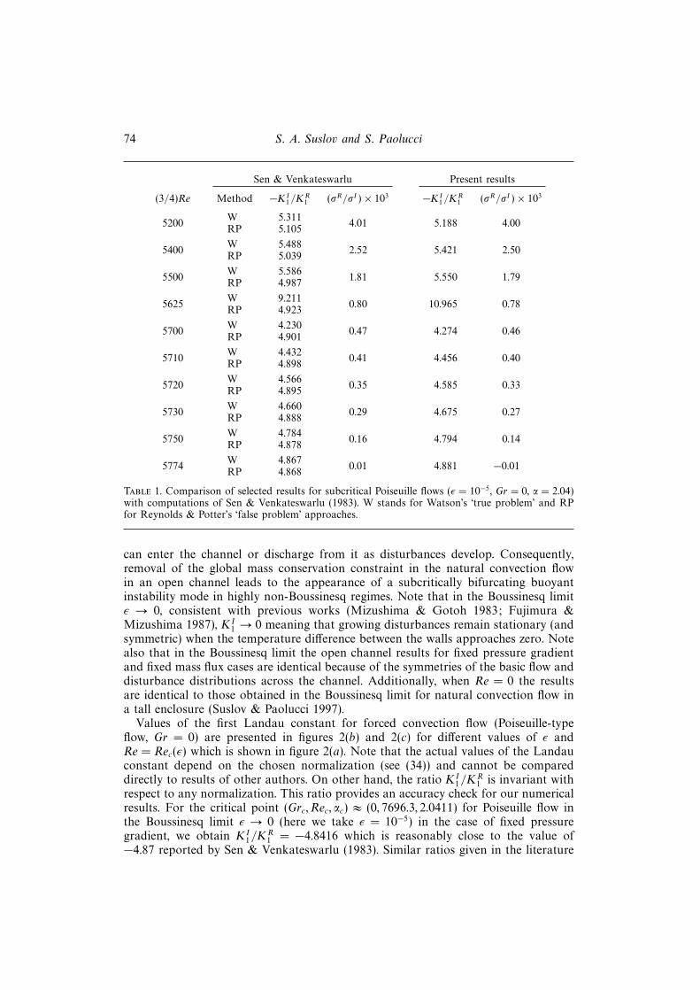
Table 1. Comparison of selected results for subcritical Poiseuille flows (ε = 10−5, Gr = 0, α = 2.04)with computations of Sen & Venkateswarlu (1983). W stands for Watson’s ‘true problem’ and RPfor Reynolds & Potter’s ‘false problem’ approaches.

can enter the channel or discharge from it as disturbances develop. Consequently,removal of the global mass conservation constraint in the natural convection flowin an open channel leads to the appearance of a subcritically bifurcating buoyantinstability mode in highly non-Boussinesq regimes. Note that in the Boussinesq limitε → 0, consistent with previous works (Mizushima & Gotoh 1983; Fujimura &Mizushima 1987), KI

1 → 0 meaning that growing disturbances remain stationary (andsymmetric) when the temperature difference between the walls approaches zero. Notealso that in the Boussinesq limit the open channel results for fixed pressure gradientand fixed mass flux cases are identical because of the symmetries of the basic flow anddisturbance distributions across the channel. Additionally, when Re = 0 the resultsare identical to those obtained in the Boussinesq limit for natural convection flow ina tall enclosure (Suslov & Paolucci 1997).

Values of the first Landau constant for forced convection flow (Poiseuille-typeflow, Gr = 0) are presented in figures 2(b) and 2(c) for different values of ε andRe = Rec(ε) which is shown in figure 2(a). Note that the actual values of the Landauconstant depend on the chosen normalization (see (34)) and cannot be compareddirectly to results of other authors. On other hand, the ratio KI

1/KR1 is invariant with

respect to any normalization. This ratio provides an accuracy check for our numericalresults. For the critical point (Grc, Rec, αc) ≈ (0, 7696.3, 2.0411) for Poiseuille flow inthe Boussinesq limit ε → 0 (here we take ε = 10−5) in the case of fixed pressuregradient, we obtain KI

1/KR1 = −4.8416 which is reasonably close to the value of

−4.87 reported by Sen & Venkateswarlu (1983). Similar ratios given in the literature


(Reynolds & Potter 1967; Davey, Hocking & Stewartson 1974; Fujimura 1989) forthe case of fixed mass flux range from −5.62 up to −5.58. To the authors’ knowledge,the most accurate value obtained in this case is that of Fujimura (1989) who givesKI

1/KR1 = −5.5832. Our value of KI

1/KR1 = −5.5838 is in very close agreement with

his result. Our results also compare favourably with those of Sen & Venkateswarlu(1983) for subcritical Poiseuille flow as can be seen from table 1. Owing to a differentnon-dimensionalization, our values for Re and α are larger than theirs by factorsof 4/3 and 2, respectively. Note that the results for the linear eigenvalue problempresented in Sen & Venkateswarlu (1983) seem to be slightly inaccurate since thevalue of the critical Reynolds number for the Poiseuille flow (Rec ≈ 5772 when thenon-dimensionalization is based on maximum speed and half of the channel width)is apparently overestimated. As a consequence, our eigenvalue results (σR/σI in table1) are presumably more accurate but differ slightly from the ones obtained by Sen &Venkateswarlu.

The values obtained for the first Landau constant (−KI1/K

R1 ) generally lie between

similar values obtained by Sen & Venkateswarlu using Watson’s (1960) ‘true prob-lem’ and Reynolds & Potter’s (1967) false problem techniques. Note that Watson’sapproach leads to a singular behaviour in the vicinity of the subcritical Reynoldsnumber value of 7533 (or 3Re/4 = 5650). Here a resonance between the mean flowcorrection induced by the fundamental mode with α = 2.04 and the α = 0 distur-bance mode occurs (see Suslov & Paolucci 1997), i.e. the condition 2σR|α= 2.04 = −π2,is satisfied, where, as can be shown in the Boussinesq limit, σn = −(n2π2) andσn = −(n2π2)/Pr, n = 1, 2, . . . are the eigenvalues of problem (33) associated withthe momentum and thermal energy equations, respectively, for α = 0 in case of fixedpressure gradient. This type of resonance limits the applicability of the one-modeanalysis of Watson in subcritical regimes (see discussions in Davey & Nguyen 1971;Herbert 1983; Sen & Venkateswarlu 1983). Although not identical, our reductionscheme is similar to Watson’s method and has similar limitations (we also obtain asingularity at the resonant point, see table 1).

Note that the analysis of subcritical flows when the average mass flux is fixed isless restricted since the eigenvalues associated with the momentum equations in theBoussinesq limit at α = 0 are −4(n2π2), n = 1, 2, . . . . Recently, the present authors(Suslov & Paolucci 1997) noted that this difficulty can be avoided within a ‘trueproblem’ approach by considering the interaction with the mean flow modes. Thiswould require derivation of a system of the coupled amplitude equations and thecorresponding coupled Landau series in the vicinity of the resonant point. Note thatthe cubic Landau equation considered in the present paper is a low-order truncationof the infinite-order Landau equation representing the temporal evolution of thedisturbance amplitude. It is accurate only if this amplitude is sufficiently small. Asdiscussed in Davey & Nguyen (1971) and Herbert (1983), when the infinite Landauseries is considered for a subcritical flow with σR < 0, it is practically impossibleto choose the governing parameters to avoid all higher-order mean flow resonances.The single-mode infinite Landau series is inevitably divergent since at least one of itscoefficients becomes infinite (see figure 2c, d in Suslov & Paolucci 1997) as a reflectionof inherently multimode interaction during the decay of disturbances.

Thus, in general, the infinite system of coupled Landau equations is necessaryto describe adequately the physics of subcritical flows and to derive correspondingconvergent Landau series. On the other hand it is relatively easy to locate the lowest-order resonant points (there exists only a finite number of them) and consider thedynamics in the parameter ranges away from them. In this case the Landau equations


would be necessary to define only the higher order Landau constants which aremultiplied by higher powers of the amplitude in the infinite coupled Landau series.If the disturbance amplitude is sufficiently small, neglecting these higher-order termsin the infinite Landau series (now convergent with finite coefficients obtained fromthe mode coupling) would not lead to a large error. It can be shown then that thecubic Landau equation obtained by the low-order truncation of the infinite-ordercoupled Landau equations is identical to the one derived from a single-mode analysisdiscussed in detail in this paper if the first mean flow resonance occurs at the order|A|4 or higher (see also discussion on page 18 in Suslov & Paolucci 1997). Thus inthe present paper we will report results only for regions away from the lowest-orderresonances assuming that the disturbance amplitude is small enough so that thederived cubic Landau equation is a reasonable approximation of the infinite-ordercoupled Landau equations. This assumption has a simple physical interpretation.While for the fundamental disturbance mode the decay rate is σR < 0, for thedisturbance resonating with the mean flow mode it is much faster, 2mσR, m > 1. Inorder for this resonant interaction to have a noticeable effect, the initial amplitudeof the resonant mode must be large enough to persist for sufficiently long time. Ifthe amplitude is small, then the mode decays so quickly that the contribution dueto the resonance is negligible. The general indication that higher-order resonancesmay not affect strongly the qualitative behaviour of the solution can be found in theliterature (see, for example, Glendinning 1984); however, further investigation of thistheoretical aspect is required.

We should note that on the surface, the ‘false problem’ approach suggested byReynolds & Potter circumvents the difficulties mentioned above and thus one is ableto estimate the Landau constant in subcritical regimes. The fact that no singularitiesarise in this method is typically used as an argument for the superiority of this methodfor subcritical flows (see, for example, Sen & Venkateswarlu 1983). On other hand, thefailure of Watson’s approach indicates the presence of a strong mean flow interactionamong the decaying disturbances, a mechanism which does not play an importantrole in supercritical flows. By its nature, Reynolds & Potter’s approach does not takethis interaction into account. As shown in Suslov & Paolucci (1997), coexistence ofdifferent disturbance modes, even in the case when their linear amplification (or decay)rates are substantially different, could lead to a stable mixed state with equilibriumamplitudes different from the ones predicted by the one-mode analysis. Moreover, theresults obtained by Sen & Venkateswarlu (1983) for Poiseuille flow using Reynolds &Potter’s approach are not in a good agreement with the available experimental databy Nishioka et al. (1975) (see the discussion in the next subsection). Thus we chooseto stay with the Watson-type reduction scheme, which from our point of view retainsmore physical features of the original problem.

As seen from figure 2, the value of KR1 remains positive and increases monotonically

with ε. Thus, the forced convection flow, although substantially stabilized according tolinear theory, always bifurcates subcritically, and, consequently, higher-order expan-sions are necessary to give an adequate Landau model for such a flow. Note that linescorresponding to the fixed average pressure gradient and to the fixed average massflux conditions in figure 2(b) are very close to each other and cannot be distinguishedin the figure. Figure 3 presents the results for mixed convection in the Boussinesq limitε→ 0 (for which ε = 0.005 is taken in our computations). Since in the Boussinesq limitthe results are symmetric with respect to the inversion of the sign of the Reynoldsnumber, only values for Re > 0 are presented. From figure 3(b) we see that thebifurcation in the Boussinesq mixed convection flow remains supercritical along line


1

(×105)

Unstable

Stable

1050

Re

Grc

(a)

KR1

1050

(b)5

–10

105

(c)

–2

0

KI1

0

–5

3

2

(×105)

0

(×105)

(×103)

2

31

(×103)

Re

1

3 22′

2

2′

(×103)

Re

2′

2

2

2′3

1

4

Figure 3. (a) Critical Grashof number, and (b) real and (c) imaginary parts of the first Landauconstant as functions of Reynolds number for mixed convection flow in the Boussinesq limit (ε→ 0).Solid and dashed lines in (b) and (c) represent cases with ∂Π/∂y = const and m = const conditions,respectively. A discussion of the labelled points is given in the text.

1

(×105)

Unstable

Stable

40–4

Re

Grc

(a)

KR1

40–4

(b)0

–6

40

(c)

–4

2KI

1

–4

–4

3

2

(×104)

–2

(×105)

(×103) (×103)

Re(×103)

Re

Stable

4

–2

0

4

5 6

Figure 4. (a) Critical Grashof number, and (b) real and (c) imaginary parts of the first Landauconstant as functions of Reynolds number for mixed convection flow in the non-Boussinesq regimewith ε = 0.3. Solid and dashed lines in (b) and (c) represent cases with ∂Π/∂y = const andm = const conditions, respectively.

1–2 (point 1 represents natural convection) up to |Re| ≈ 1.12×104 (|Re| ≈ 1.17×104)when the pressure gradient (mass flux) is kept fixed. For Poiseuille-type flows (line3–2) the situation is the opposite: the bifurcation is subcritical for purely forcedconvection (point 3) and changes to supercritical as the Grashof number increases.From figure 4 we see that the symmetry is completely broken in the non-Boussinesqregime at ε = 0.3. The bifurcation remains supercritical for negative and relativelysmall positive Reynolds numbers and becomes subcritical for Re & 3400 (Re & 4900)when the force associated with the applied pressure gradient opposes the buoyancyin the region close to the cold wall, where the disturbance maximum is located (seeSuslov & Paolucci 1995b, 1997 for details). Thus the range of Reynolds numberswhere the cubic Landau equation models the complete dynamics of the disturbancesadequately becomes substantially smaller when fluid properties are allowed to varywith temperature.

From figures 1–4 we notice that for fixed ε and Re the value of |KR1 | obtained for

the case of fixed average pressure gradient is generally smaller than the correspondingvalue for the case of fixed average mass flux. Since the magnitude of the equilibrium


4′

(×105)

Unstable

Stable

200–20

Re

Grc

(a)

KR1

200–20

(b)

0

–4

200

(c)–2.0

–0.5

KI1

–20

–3

0

(×107)

–2

(×107)

(×103) (×103)

Re(×103)

Re

20

–1.5

–1.0

Unstable 42

15

0.012

4

4′

5

3

–1

12

4

4′5

3

3

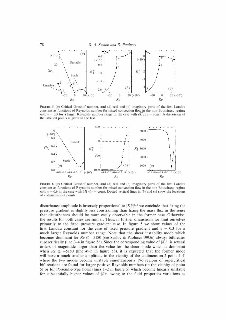
Figure 5. (a) Critical Grashof number, and (b) real and (c) imaginary parts of the first Landauconstant as functions of Reynolds number for mixed convection flow in the non-Boussinesq regimewith ε = 0.3 for a larger Reynolds number range in the case with ∂Π/∂y = const. A discussion ofthe labelled points is given in the text.

(×105)

Unstable

Stable

–0.6–0.8

Re

Grc

(a)

KR1

(b)

5000

1000 (c)–1000

0

KI1

2000

0.0

3000

(×103) (×103)

Re(×103)

Re

0.2

–500

500

40000.8

1.0

0.6

0.4

–0.4 –0.2 0 –0.6–0.8 –0.4 –0.2 0 –0.6–0.8 –0.4 –0.2 0

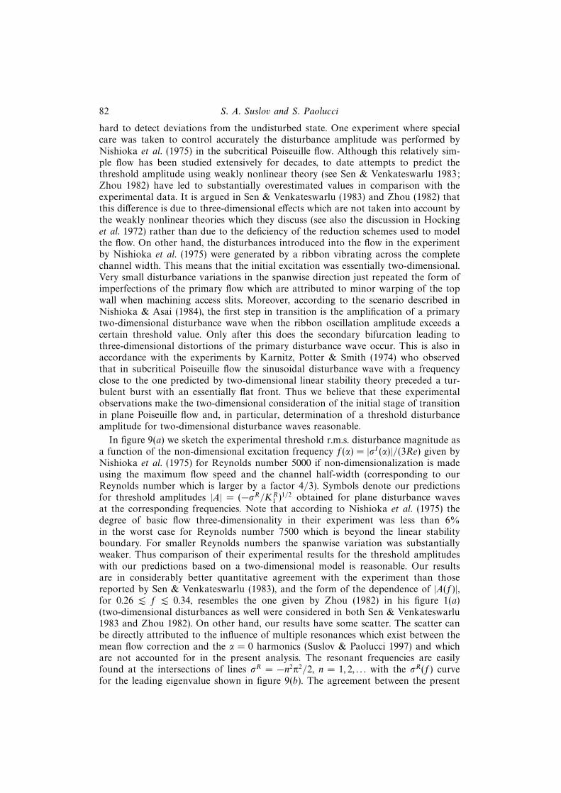
Figure 6. (a) Critical Grashof number, and (b) real and (c) imaginary parts of the first Landauconstant as functions of Reynolds number for mixed convection flow in the non-Boussinesq regimewith ε = 0.6 in the case with ∂Π/∂y = const. Dotted vertical lines in (b) and (c) show the locationsof codimension-2 points.

disturbance amplitude is inversely proportional to |KR1 |1/2 we conclude that fixing the

pressure gradient is slightly less constraining than fixing the mass flux in the sensethat disturbances should be more easily observable in the former case. Otherwise,the results for both cases are similar. Thus, in further discussions we limit ourselvesprimarily to the fixed pressure gradient case. In figure 5 we show values of thefirst Landau constant for the case of fixed pressure gradient and ε = 0.3 for amuch larger Reynolds number range. Note that the shear instability mode whichbecomes dominant for Re . −5180 (see Suslov & Paolucci 1995b) always bifurcatessupercritically (line 3–4 in figure 5b). Since the corresponding value of |KR

1 | is severalorders of magnitude larger than the value for the shear mode which is dominantwhen Re & −5180 (line 4′–5 in figure 5b), it is expected that the former modewill have a much smaller amplitude in the vicinity of the codimension-2 point 4–4′where the two modes become unstable simultaneously. No regions of supercriticalbifurcations are found for larger positive Reynolds numbers (in the vicinity of point5) or for Poiseuille-type flows (lines 1–2 in figure 5) which become linearly unstablefor substantially higher values of |Re| owing to the fluid properties variations as


(×105)Unstable

Stable

Re

Grc

(a)

KR1

(b)

0

–1.0

(c)0

KI1

–0.8

0

–0.6

(×103) Re

2

2

–0.26

4

–5 0 5 10

Stable

Re (×103)–5 0 5 10

(×106)

(×103)–5 0 5 10

–0.4

(×107)

Figure 7. (a) Critical Grashof number, and (b) real and (c) imaginary parts of the first Landauconstant as functions of Reynolds number for mixed convection flow in the non-Boussinesq regimewith ε = 0.6 for a larger Reynolds number range in the case with ∂Π/∂y = const.

discussed in Suslov & Paolucci (1995b). Note also that points 1 and 5 in figure 5are equivalent to each other since they represent the same purely forced flow profiles(Gr = 0), but with velocities in opposite directions.

In the strongly non-Boussinesq regime with ε = 0.6, the buoyant instability modediscussed in Suslov & Paolucci (1995b) bifurcates supercritically for Re . −10. Asseen from figure 6, this range covers a substantial part of the region where, accordingto linear theory, it dominates the shear-driven instability. The shear mode alwaysbifurcates subcritically as seen from figure 7. Note that lines similar to 2–3 in figure3 and 1–2 in figure 5 which correspond to dominant forced convection are not pre-sented in figures 6 and 7 since the linear instability in this case occurs at extremelylarge Reynolds numbers (see figure 2 and Suslov & Paolucci 1995b). Summarizing, weconclude that the non-Boussinesq effects have a strong influence on the stability char-acteristics of the primary flow. Not only do the values of critical parameters predictedby linear stability analysis deviate substantially from the Boussinesq predictions, butalso the character of bifurcation changes qualitatively as the temperature differencebetween the walls increases.

4.2. Disturbance amplitudes

While the periodic disturbances discussed in Suslov & Paolucci (1995b) and meanflow correction distributions (see Part 2) represent the spatial form of the flow fieldsbeyond the bifurcation, they do not provide any information on the actual size ofthe disturbances or on how the disturbances develop. Thus in this section we analysethe solutions for the disturbance amplitude satisfying the Landau equation (55). Thecurrent reduction scheme enabled us to derive the Landau equation which governs thedynamics of the disturbance amplitude away from the bifurcation point. Typically, inweakly nonlinear theory, when the relative distance from the critical point is takenas a small expansion parameter, the constants entering the Landau equation areevaluated at the critical point. Then the equilibrium amplitude for a disturbance waveis estimated as∣∣∣∣ σR(δ)

KR1 (δ = 0)

∣∣∣∣1/2 , where δ = (Re/Rec − 1)∣∣∣ε, Gr fixed

or δ = (Gr/Grc − 1)∣∣∣ε, Re fixed


Long wave(shear instability)

δ

ae

(c)

0

0.02

0 0.05 0.150.10

Short wave(shear instability)

Long wave(buoyant instability)

δ

(d )

0

0.02

0 0.05 0.150.10


0.04

Shear instabilityae

(a)0

0.010

–0.15 –0.10 0–0.05

ε = 0.3


0

0.010

–0.15 –0.10 0–0.05

Long wave(shear instability)

ε = 0.005

(b)

0.0050.005

Figure 8. Bifurcation diagrams for disturbance waves for ∂Π/∂y = const and (a) Poiseuille-typeflows (ε, Re, Gr) = (0.005, 7700, 0) and (ε, Re, Gr) = (0.3, 25960, 0), and codimension-2 pointsat (b) (ε, Re, Gr) = (0.005, 12850, 442730), (c) (ε, Re, Gr) = (0.3,−5150, 524640), and (d)(ε, Re, Gr) = (0.6,−860, 95032). Dotted lines represent the approximate bifurcation diagrams ob-tained using the value of the first Landau constant at the corresponding critical points (δ = 0).

for Poiseuille-type flows and for natural or mixed convection flows, respectively. Inthis approach one implicitly assumes that the Landau constant does not change withδ. From figure 8 we see that this is not the case in general. Thus, a conclusion we drawin analysing the bifurcation diagrams in figure 8 is that one should be careful whentrying to sum the higher-order terms in the Stuart–Landau series in order to predictan equilibrium amplitude away from the bifurcation point as done, for instance, inSen & Venkateswarlu (1983). The correction due to the higher-order terms in theStuart–Landau series in some cases can be of the same order as the error introducedwhen the variation of the Landau constants with δ is neglected.

The bifurcation diagrams presented in figure 8 show the equilibrium amplitudeswhen the bifurcations are supercritical, and the threshold amplitudes which limitthe basin of attraction of the undisturbed parallel flow when the bifurcations aresubcritical, both for periodic wave disturbances with wavenumbers correspondingto those of maximum linear growth rate. Values of critical parameters were found


in our earlier work on linear stability of mixed convection flow (Suslov & Paolucci1995b). From figure 8(a) we conclude that Poiseuille-type flows become much moresensitive to the size of disturbances when the temperature difference is increasedsince the threshold amplitude is substantially decreased. The threshold amplitudecorresponding to ε = 0.3 is difficult to obtain for larger values of |δ| because a meanflow resonance (Suslov & Paolucci 1997) occurs just beyond the curve truncationpoint in the figure. The situation is even worse for the mixed convection flow in thevicinity of the codimension-2 point in the Boussinesq limit (as discussed in Suslov &Paolucci 1995b), two different shear instability modes with α = 1.6815 and α = 2.1074compete here) which is shown in figure 8(b): the influence of the mean flow resonanceextends very close to the bifurcation point such that only the approximate valuesof the threshold amplitudes based on the Landau constant estimated for δ = 0 arepresented for the subcritically bifurcating short-wavelength instability mode. Notethat although the values of δ are negative, the long-wavelength instability bifurcatessupercritically (KR

1 < 0 as can be seen from figure 3b). The negative values of δ arisesince the flow is destabilized when the value of the Grashof number is decreasedbelow Grc (down from point 2 and below line 2–3 in figure 3a). Figure 8(b) indicatesthat the equilibrium long-wavelength disturbance amplitude remains smaller than thethreshold amplitude for the shorter wave. This fact suggests that the longer waveshould represent a stable state in the vicinity of the codimension-2 point in theBoussinesq limit, although mode coupling must be taken into account to completethe investigation of pattern selection (see Suslov & Paolucci 1997). From figure 8(c)we see that at ε = 0.3 two shear modes (see Suslov & Paolucci 1995b) bifurcatesupercritically in the vicinity of the codimension-2 point (our computations showthat KR < 0 at points 4 and 4′ in figure 5b). Again the long shear instability wave(α = 0.0800) is expected to play a dominant role since it is characterized by a muchlarger equilibrium amplitude than that for the short wave (α = 1.1828). However, thiscan only be confirmed by examining the coupled equations near the codimension-2point, which is beyond the scope of the present work. The short-wave disturbanceequilibrium amplitude is smaller since the dissipation is more intense for smallercells. From figure 8(d) we see that in the strongly non-Boussinesq regime at ε = 0.6,the interaction is between the shear (α = 0.6285) and buoyant (α = 0.1000) modes(see Suslov & Paolucci 1995b). For the downward flow the former is subcritical andthe latter is supercritical (see figures 6b and 7b), while for the upward flow bothbifurcations are subcritical. The individual bifurcation diagrams shown in figure 8(d)for the codimension-2 point correspond to the downward flow case. It is expectedthat for Grashof numbers smaller than the critical value, sufficiently large initialdisturbances will lead to the shear type of instability. For larger Grashof numbers,the basic flow could initially be destabilized by buoyant disturbances which could thenexcite the shear instability so that finally it becomes dominant or leads to some mixedstate depending on the specific choice of parameters. The codimension-2 analysis canbe performed by deriving the coupled Landau equations as in Suslov & Paolucci(1997). This has not been done at this point.

Evaluations of equilibrium disturbance amplitudes are necessary in order to quanti-tatively predict such important characteristics of the disturbed flow as the average heattransfer rate or the average mass flux. Thus, it is instructive to compare predictionsbased on the proposed reduction scheme with experimental results. Unfortunately,experiments in the vicinity of criticality, where weakly nonlinear theory is most ac-curate, are generally very difficult to perform owing to very small and, consequently,


hard to detect deviations from the undisturbed state. One experiment where specialcare was taken to control accurately the disturbance amplitude was performed byNishioka et al. (1975) in the subcritical Poiseuille flow. Although this relatively sim-ple flow has been studied extensively for decades, to date attempts to predict thethreshold amplitude using weakly nonlinear theory (see Sen & Venkateswarlu 1983;Zhou 1982) have led to substantially overestimated values in comparison with theexperimental data. It is argued in Sen & Venkateswarlu (1983) and Zhou (1982) thatthis difference is due to three-dimensional effects which are not taken into account bythe weakly nonlinear theories which they discuss (see also the discussion in Hockinget al. 1972) rather than due to the deficiency of the reduction schemes used to modelthe flow. On other hand, the disturbances introduced into the flow in the experimentby Nishioka et al. (1975) were generated by a ribbon vibrating across the completechannel width. This means that the initial excitation was essentially two-dimensional.Very small disturbance variations in the spanwise direction just repeated the form ofimperfections of the primary flow which are attributed to minor warping of the topwall when machining access slits. Moreover, according to the scenario described inNishioka & Asai (1984), the first step in transition is the amplification of a primarytwo-dimensional disturbance wave when the ribbon oscillation amplitude exceeds acertain threshold value. Only after this does the secondary bifurcation leading tothree-dimensional distortions of the primary disturbance wave occur. This is also inaccordance with the experiments by Karnitz, Potter & Smith (1974) who observedthat in subcritical Poiseuille flow the sinusoidal disturbance wave with a frequencyclose to the one predicted by two-dimensional linear stability theory preceded a tur-bulent burst with an essentially flat front. Thus we believe that these experimentalobservations make the two-dimensional consideration of the initial stage of transitionin plane Poiseuille flow and, in particular, determination of a threshold disturbanceamplitude for two-dimensional disturbance waves reasonable.

In figure 9(a) we sketch the experimental threshold r.m.s. disturbance magnitude asa function of the non-dimensional excitation frequency f(α) = |σI (α)|/(3Re) given byNishioka et al. (1975) for Reynolds number 5000 if non-dimensionalization is madeusing the maximum flow speed and the channel half-width (corresponding to ourReynolds number which is larger by a factor 4/3). Symbols denote our predictionsfor threshold amplitudes |A| = (−σR/KR

1 )1/2 obtained for plane disturbance wavesat the corresponding frequencies. Note that according to Nishioka et al. (1975) thedegree of basic flow three-dimensionality in their experiment was less than 6%in the worst case for Reynolds number 7500 which is beyond the linear stabilityboundary. For smaller Reynolds numbers the spanwise variation was substantiallyweaker. Thus comparison of their experimental results for the threshold amplitudeswith our predictions based on a two-dimensional model is reasonable. Our resultsare in considerably better quantitative agreement with the experiment than thosereported by Sen & Venkateswarlu (1983), and the form of the dependence of |A(f)|,for 0.26 . f . 0.34, resembles the one given by Zhou (1982) in his figure 1(a)(two-dimensional disturbances as well were considered in both Sen & Venkateswarlu1983 and Zhou 1982). On other hand, our results have some scatter. The scatter canbe directly attributed to the influence of multiple resonances which exist between themean flow correction and the α = 0 harmonics (Suslov & Paolucci 1997) and whichare not accounted for in the present analysis. The resonant frequencies are easilyfound at the intersections of lines σR = −n2π2/2, n = 1, 2, . . . with the σR(f) curvefor the leading eigenvalue shown in figure 9(b). The agreement between the present


f

σR

(b)

–8000.20 0.25 0.30 0.35 0.40

–600

–400

–200

0

√2|A|

(a)

0.01

0.20 0.25 0.30

0.02

0.03

0.04

0.35 0.40

Figure 9. (a) Disturbance threshold amplitude curve from Nishioka et al. (1975); symbols denotevalues predicted by the present analysis. (b) Plane wave linear decay rate σR as a function ofnon-dimensional frequency for the Poiseuille flow at Re = 4/3 × 5000; intersections of σR =−n2π2/2 (n = 1, 2, . . .) lines and the σR(f) curve represent resonance points.

theoretical results and the experimental results in resonance-free frequency intervalsis satisfactory, and thus we expect that our predictions for supercritical (σR(α) > 0)flows, where no mean flow resonances exist, are sufficiently accurate.

Note also that the theory developed in Suslov & Paolucci (1997) enables oneto model the evolution of a disturbance wave not necessarily corresponding to thewavenumber α (or frequency f) of the maximum linear amplification rate σR . In otherwords disturbance quantities can be computed and expansions can be made basedon eigenfunctions of the linearized problem whose spatial period (and frequencyof oscillation) differ from the critical ones. This enables us to consider a forcedsystem where the frequency of the disturbances is prescribed by external means.Our calculations of KR

1 for Poiseuille flow at Re = 4/3 × 5000 (not presented here)show that it becomes negative for f . 0.22 and f & 0.40, which means that planewave disturbances at these frequencies must decay no matter how big their initialamplitudes are. Thus, consistent with figure 10 in Sen & Venkateswarlu (1983), thepredicted threshold amplitude increases rapidly outside the interval 0.22 . f . 0.40,and no threshold amplitudes are computed for frequencies beyond this range asshown in figure 9a). The decrease in the experimental threshold amplitude outsidethis frequency range can be attributed to the development of localized rather thanperiodic disturbances. Turbulent spots in the laminar flow were observed in theexperiment by Nishioka et al. (1975) in this frequency range, but they cannot bemodelled within a discrete wave approach and require consideration of spatiallymodulated disturbance waves and wave packets.


5. SummaryWe have developed a weakly nonlinear theory for the analysis of flows in open

domains where the total mass of fluid might not be conserved. The theory is appliedto the non-Boussinesq mixed convection flow of air in an open vertical channel withdifferentially heated walls. It is shown that constant mass flux and constant pressuregradient formulations result in distinct problems, which lead to qualitatively similarbut quantitatively different results. The cubic Landau equation is shown to modelthe evolution of the disturbance amplitude for a wide range of governing parameters.Based on this equation the regions of supercritical and subcritical bifurcations areidentified. Comparison of the present theory with those developed by Watson (1960)and Reynolds & Potter (1967) demonstrates the advantage of the current approachwhich is capable of providing better quantitative predictions for super- and subcriticalflow regimes further from the marginally stable state.

AppendixFunctions entering the right-hand side of (45):

f(1)20 = − 8

3Re {D(µ11 Du∗11)}+ 2α Im { 2

3D(µ11v

∗11)− ρ00u11v

∗11 + ρ11u

∗11v00}

+ ρ00 D|u11|2 + 2Re {σρ∗11u11},f

(2)20 = 2Re {ρ00u11 Dv∗11 + ρ11u

∗11 Dv00 −D(µ11 Dv∗11)}+ 2α Im {ρ11v

∗11v00 −D(µ11v

∗11)}

+Π20 −D(µ00TT |T11|2 Dv00) +Gr

2ερ00TT |T11|2 + 2Re {σρ∗11v11},

f(3)20 = 2Re

{cp00(ρ00 DT11u

∗11 + ρ11 DT00u

∗11) + cp11ρ00 DT00u

∗11 − 1

PrD(k11DT

∗11)

}+ 2αcp00Im {cp00(ρ11T

∗11v00 − ρ00T11v

∗11) + cp11ρ00T

∗11v00}

− 1

PrD(k00TT |T11|2 DT00) + 2Re {σ(cp00ρ

∗11 + c∗p11ρ00)T11},

f(4)20 = −2Re {D(ρ11u

∗11)}+ 2σRρ00TT |T11|2,

where for the variable properties used

cp11 = cp20 = cp22 = 0, ρ00TT ≡ ∂2ρ00

∂T 200

= 2ρ00

T 200

,

µ00TT ≡ ∂2µ00

∂T 200

= −1 + Sµ

4

T 200 + 6SµT00 − 3S2

µ√T00(T00 + Sµ)3

,

k00TT ≡ ∂2k00

∂T 200

= −1 + Sk

4

T 200 + 6SkT00 − 3S2

k√T00(T00 + Sk)3

.

REFERENCES

Chenoweth, D. R. & Paolucci, S. 1985 Gas flow in vertical slots with large horizontal temperaturedifferences. Phys. Fluids 28, 2365–2374.

Chenoweth, D. R. & Paolucci, S. 1986 Natural convection in an enclosed vertical air layer withlarge horizontal temperature differences. J. Fluid Mech. 169, 173–210.

Davey, A., Hocking, L. & Stewartson, K. 1974 On the nonlinear evolution of three-dimensionaldisturbances in plane Poiseuille flow. J. Fluid Mech. 63, 529–536.


Davey, A. & Nguyen, H. P. F. 1971 Finite-amplitude stability of pipe flow. J. Fluid Mech. 45,701–720.

Frohlich, J., Laure, P. & Peyret, R. 1992 Large departures from Boussinesq approximation in theRayleigh–Benard problem. Phys. Fluids 4, 1355–1371.

Fujimura, K. 1989 The equivalence between two perturbation methods in weakly nonlinear stabilitytheory for parallel shear flows. Proc. R. Soc. Lond. A 424, 373–392.

Fujimura, K. & Mizushima, J. 1987 Nonlinear interaction of disturbances in free convectionbetween vertical parallel plates. In Nonlinear Wave Interactions in Fluids (ed. R. W. Miksad,T. R. Akylyas & T. Herbert), pp. 123–130.

Glendinning, P. 1984 Stability, Instability and Chaos: an Introduction to the Theory of NonlinearDifferential Equations, pp. 78–83. Cambridge University Press.

Herbert, T. 1983 On perturbation methods in nonlinear stability theory. J. Fluid Mech. 126, 167–186.

Hocking, L., Stewartson, K., Stuart, J. T. & Brown, S. N. 1972 A nonlinear instability burst inplane parallel flow. J. Fluid Mech. 51, 705–735.

IMSL, Inc. 1989 IMSL Mathematical Library, Version 1.1. Houston, TX.

Karnitz, M., Potter, M. & Smith, M. 1974 An experimental investigation of transition of a planePoiseuille flow. Trans. ASME I: J. Fluids Engng 96, 384–388.

Mizushima, J. & Gotoh, K. 1983 Nonlinear evolution of the disturbance in a natural convectioninduced in a vertical fluid layer. J. Phys. Soc. Japan 52, 1206–1214.

Nishioka, M. & Asai, M. 1984 Evolution of Tollmien–Schlichting waves. In Turbulence and ChaoticPhenomena in Fluids (ed. T. Tatsumi), pp. 87–92. Elsevier.

Nishioka, M., Iida, S. & Ichikawa, Y. 1975 An experimental investigation of the stability of planePoiseuille flow. J. Fluid Mech. 72, 731–751.

Paolucci, S. 1982 On the filtering of sound from the Navier–Stokes equations. Tech. Rep. SAND82-8257. Sandia National Laboratories, Livermore, California.

Reynolds, W. C. & Potter, M. C. 1967 Finite-amplitude instability of parallel shear flows. J. FluidMech. 27, 465–492.

Sen, P. K. & Venkateswarlu, D. 1983 On the stability of plane Poiseuille flow to finite-amplitudedisturbances, considering higher-order Landau coefficients. J. Fluid Mech. 133, 179–206.

Stewartson, K. & Stuart, J. T. 1971 A non-linear instability theory for a wave system in planePoiseuille flow. J. Fluid Mech. 48, 529–545.

Stuart, J. T. 1960 On the non linear mechanics of wave disturbances in stable and unstable parallelflows. Part 1. The basic behaviour in plane Poiseuille flow. J. Fluid Mech. 9, 353–370.

Suslov, S. A. 1997 Nonlinear analysis of non-Boussinesq convection. PhD thesis, University ofNotre Dame, USA.

Suslov, S. A. & Paolucci, S. 1995a Stability of natural convection flow in a tall vertical enclosureunder non-Boussinesq conditions. Intl J. Heat Mass Transfer 38, 2143–2157.

Suslov, S. A. & Paolucci, S. 1995b Stability of mixed-convection flow in a tall vertical channelunder non-Boussinesq conditions. J. Fluid Mech. 302, 91–115.

Suslov, S. A. & Paolucci, S. 1997 Nonlinear analysis of convection flow in a tall vertical enclosureunder non-Boussinesq conditions. J. Fluid Mech. 344, 1–41.

Suslov, S. A. & Paolucci, S. 1999 Nonlinear stability of mixed convection flow under non-Boussinesq conditions. Part 2. Mean flow characteristics. J. Fluid Mech. 398, 87–108.

Watson, J. 1960 On the non-linear mechanics of wave disturbances in stable and unstable parallelflows. Part 2. The development of a solution for plane Poiseuille flow and for plane Couetteflow. J. Fluid Mech. 9, 371–389.

White, F. M. 1974 Viscous Fluid Flow. McGraw-Hill.

Yao, L. S. & Rogers, B. B. 1992 Finite-amplitude instability of non-isothermal flow in verticalannulus. Proc. R. Soc. Lond. A 437, 267–290.

Zhou, H. 1982 On the non linear theory of stability of plane Poiseuille flow in the subcritical range.Proc. R. Soc. Lond. A 381, 407–418.

nonlinear stability of mixed convection flow under non … · nonlinear stability of mixed...

Documents