nonlinear vector network analyzer applications - … · nonlinear vector network analyzer...
TRANSCRIPT

Nonlinear Vector Network Analyzer Applications- The PNA-X as NVNA for extracting X-Parameters -
presented by:Dr Marc LECOUVE
from original Slideset created by:Dr. David E. Root, Principal Research Scientist & Loren Betts, Research Scientist
Agilent Technologies

…Evolution of the Tools & Measurements
TOOLS:
S-Parameters
TOOLS:
S-Parameters +Figures of Merit
TOOLS:
Patchwork
NVNA +X-Parameters
TOOLS:
VNA
SA/SS/NFAPower meter
TOOLS:
Vector NetworkAnalyzer
MEASUREMENTS:
TOOLS:
SS & OscilloscopeGrease pens and
Polaroid cameras Power meter
Oscilloscope
DC Parametric Analyzer
MEASUREMENTS:
Gain
Input match
Output match
Polaroid cameras
Slotted line
Power meter
Scalar network analyzers
MEASUREMENTS:
Gain compression, IP3, IMD
PAE, ACPR, AM-PM, BER
Output match
Isolation
Transconductance
Input capacitance
MEASUREMENTS:
Bode plots
GainConstellation Diagram, EVM
GD, NF, Spectral Regrowth
ACLR, Hot “S22”
Input capacitanceGain
SWR
Y & Z parameters
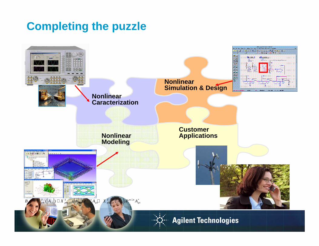
Completing the puzzle
Nonlinear Caracterization
Nonlinear Simulation & Design
Nonlinear Modeling
Customer ApplicationsNonlinear
ModelingApplications
*( ) ( ) ( )F S m n T m nB X A X A P A X A P A− += + + *11 , 11 , 11( ) ( ) ( )F S m n T m n
pm pm pm qn qn pm qn qnB X A X A P A X A P A− += + +
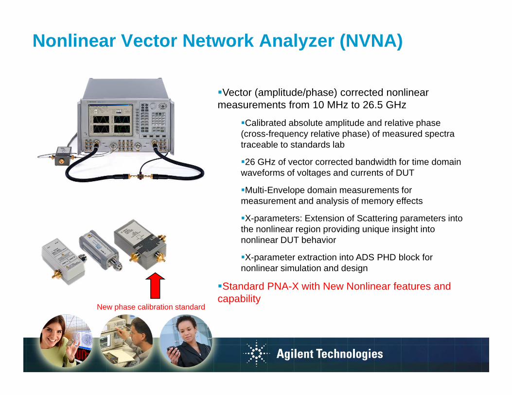
Nonlinear Vector Network Analyzer (NVNA)
Vector (amplitude/phase) corrected nonlinear measurements from 10 MHz to 26.5 GHz
Calibrated absolute amplitude and relative phase Calibrated absolute amplitude and relative phase (cross-frequency relative phase) of measured spectra traceable to standards lab
26 GHz of vector corrected bandwidth for time domain waveforms of voltages and currents of DUTwaveforms of voltages and currents of DUT
Multi-Envelope domain measurements for measurement and analysis of memory effects
X-parameters: Extension of Scattering parameters into X-parameters: Extension of Scattering parameters into the nonlinear region providing unique insight into nonlinear DUT behavior
X-parameter extraction into ADS PHD block for nonlinear simulation and designnonlinear simulation and design
Standard PNA-X with New Nonlinear features and capability
New phase calibration standard
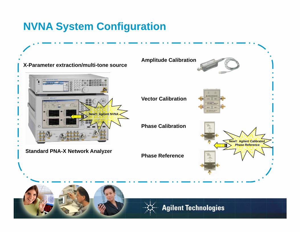
NVNA System Configuration
Amplitude CalibrationX-Parameter extraction/multi-tone source
Vector CalibrationVector Calibration
Phase Calibration
New!! Agilent NVNA
Phase ReferenceStandard PNA-X Network Analyzer
New!! Agilent Calibrated Phase Reference

NVNA Applications (What does it do?)
Time domain oscilloscope measurements with vector error correction applied
View time domain (and frequency domain) waveforms (similar to an oscilloscope) but with vector correction oscilloscope) but with vector correction applied (measurement plane at DUT terminals)
Vector corrected time domain voltages (and currents) from device

NVNA Applications (What does it do?)Measure amplitude and cross-frequency phase of frequencies to/from device with vector error correc tion frequencies to/from device with vector error correc tion applied View absolute amplitude and phase relationship
between frequencies to/from a device with vector correction applied (measurement plane vector correction applied (measurement plane at DUT terminals)
Useful to analyze/design high efficiency amplifiers such as class E/Famplifiers such as class E/F
Can also measure frequency multipliers1 GHz
Fundamental Frequency
Source harmonics (< 60 dBc)
Stimulus to device
2 GHz
Output from device
Input output frequencies at device terminals1 GHz
2 GHz
122.1 degree phase delta
Output harmonics
Phase relationship between frequencies at output of device

NVNA Applications (What does it do?)Measurement of narrow (fast) DC pulses with vector Measurement of narrow (fast) DC pulses with vector error correction applied
View time domain (and frequency domain) representations of narrow DC pulses with vector correction applied pulses with vector correction applied (measurement plane at DUT terminals)
Less than 50 ps
Note: DC signal with 250 MHz PRF

NVNA Applications (What does it do?)Measurement of narrow (fast) View time domain (and frequency Measurement of narrow (fast) RF pulses with vector error correction applied
View time domain (and frequency domain) representations of narrow RF pulses with vector correction applied (measurement plane at DUT terminals)
Using wideband mode (resolution ~ 1/BW Using wideband mode (resolution ~ 1/BW ~ 1/26 GHz ~ 40 ps)
Example: 10 ns pulse width at a 2 GHz carrier frequency. Limited by external source not NVNA. frequency. Limited by external source not NVNA. Can measure down into the picosecond pulse widths
Note: 2 GHz RF signal 10 nsec pulsed
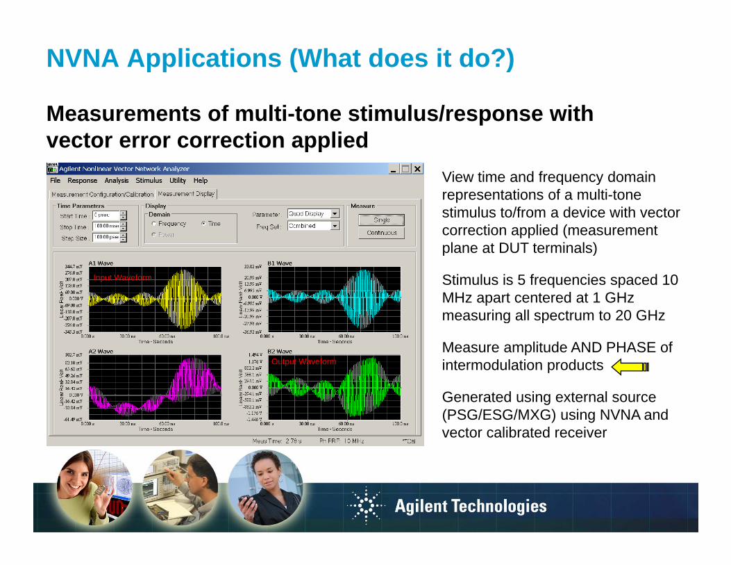
NVNA Applications (What does it do?)
Measurements of multi -tone stimulus/response with Measurements of multi -tone stimulus/response with vector error correction applied
View time and frequency domain View time and frequency domain representations of a multi-tone stimulus to/from a device with vector correction applied (measurement plane at DUT terminals)plane at DUT terminals)
Stimulus is 5 frequencies spaced 10 MHz apart centered at 1 GHz measuring all spectrum to 20 GHz
Input Waveform
measuring all spectrum to 20 GHz
Measure amplitude AND PHASE of intermodulation products
Generated using external source
Output Waveform
Generated using external source (PSG/ESG/MXG) using NVNA and vector calibrated receiver

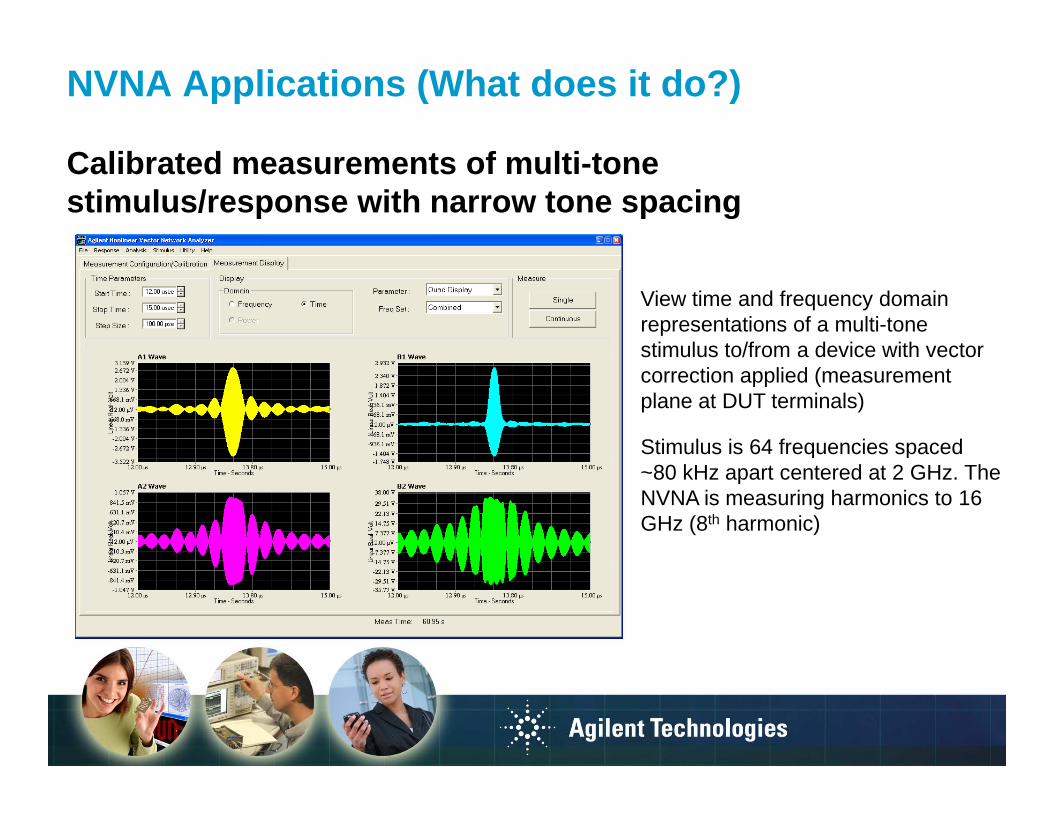
NVNA Applications (What does it do?)
Calibrated measurements of multi -tone Calibrated measurements of multi -tone stimulus/response with narrow tone spacing
View time and frequency domain View time and frequency domain representations of a multi-tone stimulus to/from a device with vector correction applied (measurement plane at DUT terminals)plane at DUT terminals)
Stimulus is 64 frequencies spaced ~80 kHz apart centered at 2 GHz. The NVNA is measuring harmonics to 16 NVNA is measuring harmonics to 16 GHz (8th harmonic)
Multi-tone often used to mimic more complex modulation (i.e. CDMA) by complex modulation (i.e. CDMA) by matching complementary cumulative distribution function (CCDF). Multi-tone can be measured very accurately.accurately.
NVNA Applications (What does it do?)
Calibrated measurements of multi -tone Calibrated measurements of multi -tone stimulus/response with narrow tone spacing
View time and frequency domain representations of a multi-tone stimulus to/from a device with vector stimulus to/from a device with vector correction applied (measurement plane at DUT terminals)
Stimulus is 64 frequencies spaced Stimulus is 64 frequencies spaced ~80 kHz apart centered at 2 GHz. The NVNA is measuring harmonics to 16 GHz (8th harmonic)
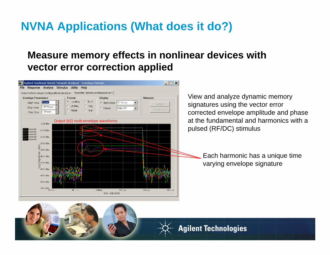
NVNA Applications (What does it do?)
Measure memory effects in nonlinear devices with vector error correction applied
View and analyze dynamic memory signatures using the vector error corrected envelope amplitude and phase corrected envelope amplitude and phase at the fundamental and harmonics with a pulsed (RF/DC) stimulus
Output (b2) multi-envelope waveforms
Each harmonic has a unique time varying envelope signature

NVNA Applications (What does it do?)
Measure modeling coefficients and other nonlinear Measure modeling coefficients and other nonlinear device parameters
X-parameters
… More
Dynamic Load Line
Waveforms (‘a’ and ‘b’ waves)
Dynamic Load Line
Measure, view and simulate actual nonlinear data from your device

Nonlinearities
( )x t ( )y t
1ω 12ω1ω 13ω
0
0
0 0
20
( ) ( )
( )
b
c
j
j
y t a b e x t
c e x t
θ
θ
= +
+
0 0( )( ) j w tx t Ae φ+=0 0 0
0 0 0
( )0 0
2( )20
( ) b
c
j j t
j j t
y t a b e Ae
c e A e
θ ω φ
θ ω φ
+
+
= +
+
1 11 1
0
0
30
( )
( )dj
c e x t
d e x tθ
+
+ 0 0 0
0
3( )30
dj j t
c e A e
d e A eθ ω φ+
+
+
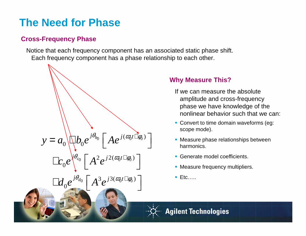
The Need for PhaseCross-Frequency Phase
Notice that each frequency component has an associated static phase shift. Each frequency component has a phase relationship to each other.
Why Measure This?
If we can measure the absolute amplitude and cross-frequency phase we have knowledge of the
( )j j tθ ω φ+ = +
phase we have knowledge of the nonlinear behavior such that we can:
Convert to time domain waveforms (eg: scope mode).
0 0 0
0 0 0
( )0 0
2( )20
b
c
j j t
j j t
y a b e Ae
c e A e
θ ω φ
θ ω φ
+
+
= +
+
Measure phase relationships between harmonics.
Generate model coefficients.
0 0 0
0
3( )30
dj j t
c e A e
d e A eθ ω φ+
+
+
Measure frequency multipliers.
Etc…..
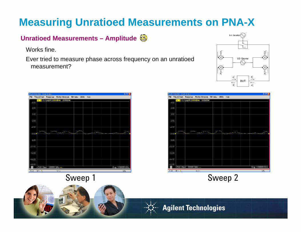
Measuring Unratioed Measurements on PNA-XUnratioed Measurements – Amplitude
Works fine.
Ever tried to measure phase across frequency on an unratioed measurement?
01a
0b
02a
0b11a
11b
12b
12a
01b 0
2b
Sweep 1 Sweep 2
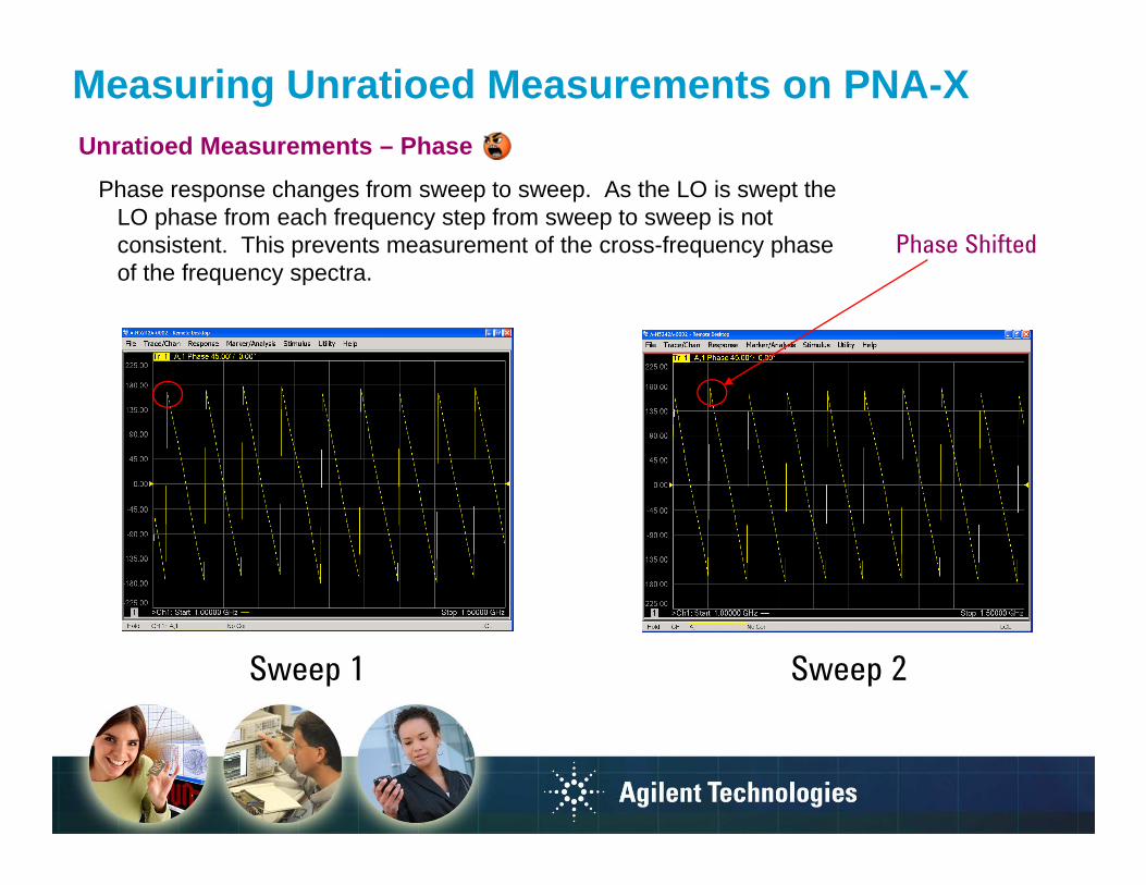
Measuring Unratioed Measurements on PNA-XUnratioed Measurements – Phase
Phase response changes from sweep to sweep. As the LO is swept the LO phase from each frequency step from sweep to sweep is not consistent. This prevents measurement of the cross-frequency phase of the frequency spectra.
Phase Shiftedof the frequency spectra.
Sweep 1 Sweep 2

NVNA Hardware ConfigurationGenerate Static Phase
Since we are using a mixer based VNA the LO phase will change as we sweep frequency. This means that we cannot directly measure the phase across frequency using unratioed (a1, b1) phase across frequency using unratioed (a1, b1) measurements.
Instead…ratio (a1/ref, b2/ref) against a device that has a constant phase relationship versus frequency. A harmonic phase reference frequency. A harmonic phase reference generates all the frequency spectrum simultaneously.
The harmonic phase reference frequency grid The harmonic phase reference frequency grid and measurement frequency grid are the same (although they do not have to be generally). For example, to measure a maximum of 5 harmonics from the device (1, 2, 3, 4, 5 GHz) you would from the device (1, 2, 3, 4, 5 GHz) you would place phase reference frequencies at 1, 2, 3, 4, 5 GHz.

NVNA Hardware ConfigurationPhase Reference
One phase reference is used to maintain a static cross-frequency phase relationship.
A second phase reference standard is A second phase reference standard is used to calibrate the cross-frequency phase at the device plane.
The phase reference generates a time The phase reference generates a time domain impulse. Fourier theory illustrates that a repetitive impulse in time generates a spectra of frequency content related to the pulse repetition content related to the pulse repetition frequency (PRF) and pulse width (PW).
The cross-frequency phase relationship remains static.

Phase Reference
New!! Agilent Calibrated
Phase Reference
Agilent’s new IC based phase reference is superior in all aspects to existing phase reference technologies.
Advantages:
Phase Reference
Lower temperature sensitivity
Lower sensitivity to input power
Smaller minimum tone spacing (< 1 MHz vs 600 MHz) Smaller minimum tone spacing (< 1 MHz vs 600 MHz)
Lower frequency (< 1 MHz vs 600 MHz)
Much wider dynamic range due to available energy vs noise1
0
0.2
0.4
0.6
0.8
Nor
ma
lized
Am
plitu
de
0 10 20 30 40 50 60 70 80 90 1000
Frequency in GHz

Frequency Domain Representation of Pulsed DC Signal
1
Frequency Response
Drive phase reference with a Fin frequency.
0.4
0.6
0.8
No
rma
lize
d A
mp
litu
de
frequency.
Get n*Fin at the output of the phase reference.
Example:
0 10 20 30 40 50 60 70 80 90 1000
0.2
Frequency in GHz
No
rma
lize
d A
mp
litu
de
Example:
Want to stimulate DUT with 1 GHz input stimulus and measure harmonic responses at 1, 2, 3, 4, 5
0.6
0.8
1
No
rma
lize
d A
mp
litu
de
responses at 1, 2, 3, 4, 5 GHz.
Fin = 1 GHz
Can practically use frequency
0
0.2
0.4
No
rma
lize
d A
mp
litu
de
Can practically use frequency spacings less than 1 MHz
0 5 10 15 20 250
Frequency in GHz
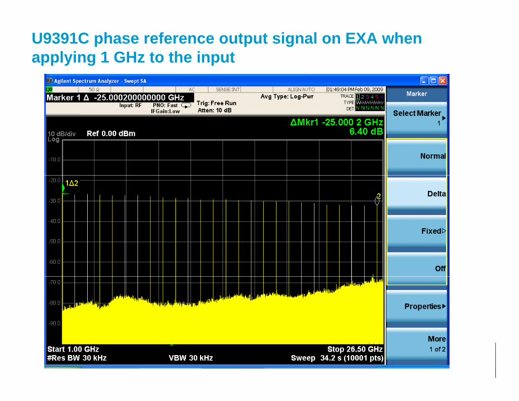
U9391C phase reference output signal on EXA when applying 1 GHz to the input

Measurement results with 500 MHz input frequencyon the U9391C harmonic phase reference.
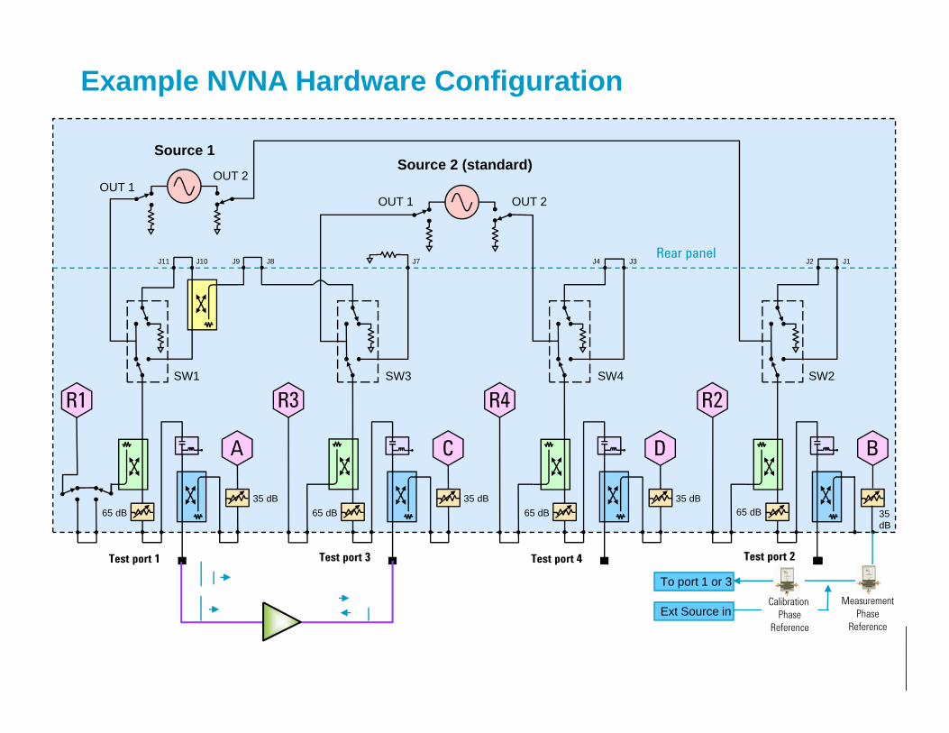
Example NVNA Hardware Configuration
Source 1
OUT 1OUT 2
Source 2 (standard)
OUT 1 OUT 2
Rear panelJ11 J10 J9 J8 J7 J4 J3 J2 J1
R3R1 R4 R2
SW1 SW3 SW4 SW2
C
35 dB 35 dB
A
35 dB
D B
Test port 3Test port 1 Test port 4 Test port 2
65 dB 65 dB 65 dB 35 dB
65 dB
To port 1 or 3
Calibration MeasurementCalibration
Phase
Reference
Ext Source inMeasurement
Phase
Reference

ADD PNA stuff from Loren BettsNVNA Demo on PNA-X

Nonlinear VNA MeasurementsStimulus/Response Setup
The user can set up a multi-The user can set up a multi-dimensional segmented sweep across input frequency and power and output response.
Single tone stimulus and harmonic response
Multi-tone stimulus/response
DC/RF pulse response
X-parameters stimulus/response
Multi-Envelope responseMulti-Envelope response

Example stimulus response setup
multidimensional sweep:1. The NVNA will set the frequency and power and measure the a and
b waves at the input and output for the fundamental frequency. b waves at the input and output for the fundamental frequency. 2. Move the receivers to the next harmonic frequency and measure
the a and b waves again. 3. When all harmonics are measured, move the power to the next
power point and measure the a and b waves for the fundamental power point and measure the a and b waves for the fundamental and all harmonics again.
4. Repeat until all power points have been measured. 5. Then move the fundamental input frequency to the next frequency 5. Then move the fundamental input frequency to the next frequency
point 6. repeat the above procedure until all the frequency points have been
measured.
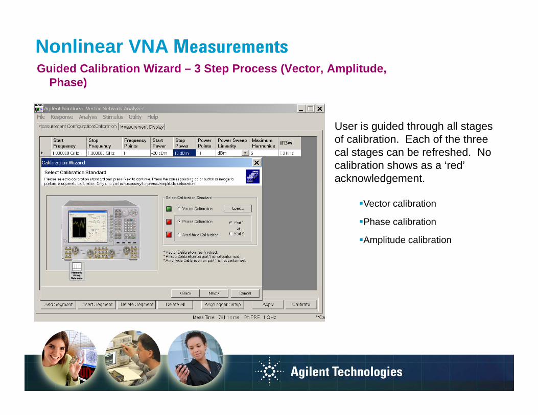
Nonlinear VNA MeasurementsGuided Calibration Wizard – 3 Step Process (Vector, Amplitude,
Phase)Phase)
User is guided through all stages User is guided through all stages of calibration. Each of the three cal stages can be refreshed. No calibration shows as a ‘red’ acknowledgement.acknowledgement.
Vector calibration
Phase calibration
Amplitude calibration

Nonlinear VNA MeasurementsGuided Calibration Wizard – Vector Calibration
The Vector calibration uses the standard PNA-X cal wizard to standard PNA-X cal wizard to generate the associated vector correction error model. Users can enter their own cal kit definitions.

Nonlinear VNA MeasurementsGuided Calibration Wizard – Phase Calibration
User is prompted to connect the User is prompted to connect the phase reference calibration standard. Standard is USB controlled. This calibrates the cross-frequency phase.cross-frequency phase.
New!New!

Nonlinear VNA MeasurementsGuided Calibration Wizard – Amplitude Calibration
User is prompted to connect the power sensor calibration standard. power sensor calibration standard. Supports any power meters/sensors the PNA-X FW supports today and in the future.

Nonlinear VNA MeasurementsMeasurement Display
The user can display the resulting corrected waves in frequency, time, corrected waves in frequency, time, power and other domains. Can also display all formats including cross-frequency phase.

Nonlinear VNA MeasurementsMeasurement Display
The vector corrected responses from the device can be displayed in time domain.

Nonlinear VNA MeasurementsMeasurement Display – Power Sweep and Phase
Can also analyze the device performance versus power. performance versus power. This example illustrates the phase of the second harmonic from the device as a function of input power.a function of input power.

Nonlinear VNA MeasurementsMeasurement Display
User can customize the displayed waveforms such as displayed waveforms such as the voltage or current applied to and emanating from the device.
‘a’ and ‘b’ waves versus sweep domain
V and I versus sweep domain
V versus I, I versus V
Etc...
Dynamic Load Line (RF I/V)

Nonlinear VNA MeasurementsIn-fixture/De-embedding
User can move the absolute User can move the absolute amplitude and cross-frequency phase plane by de-embedding S-parameters of the fixture/adapter.
Eg: Move amplitude and phase Eg: Move amplitude and phase plane (in-coax) into the fixture plane.
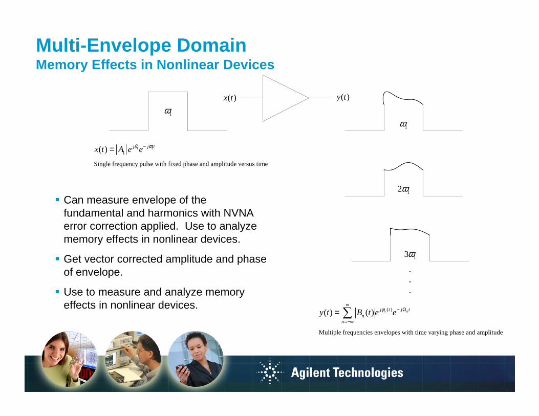
Multi-Envelope DomainMemory Effects in Nonlinear Devices
( )x t ( )y t
1ω
1ω
1 11
Single frequency pulse with fixed phase and amplitude versus time
( ) j j tx t A e eθ ω−=
1
12ω Can measure envelope of the
fundamental and harmonics with NVNA error correction applied. Use to analyze memory effects in nonlinear devices.
13ωmemory effects in nonlinear devices.
Get vector corrected amplitude and phase of envelope.
Use to measure and analyze memory ( )
Multiple frequencies envelopes with time varying phase and amplitude
( ) ( ) n nj t j tn
n
y t B t e eφ∞
− Ω
=−∞
= ∑
Use to measure and analyze memory effects in nonlinear devices.

Multi-Envelope Domain
Envelope DomainEnvelope Domain
Measure envelope of the Measure envelope of the fundamental and harmonics with NVNA error correction applied. Use to analyze memory effects in to analyze memory effects in nonlinear devices.
Get vector corrected amplitude and phase of envelope.
Envelope resolution down to 16.7 ns using narrowband detection mode.

S-parameters: linear measurement, modeling, & simulation Easy to measure at high frequencies
measure voltage traveling waves with a (linear) vector network analyzer (VNA) don't need shorts/opens which can cause devices to oscillate or self-destruct
modeling, & simulation
don't need shorts/opens which can cause devices to oscillate or self-destruct Relate to familiar measurements (gain, loss, reflection coefficient ...) Can cascade S-parameters of multiple devices to predict system performance Can import and use S-parameter files in electronic-simulation tools (e.g. ADS) BUT: No harmonics, No distortion, No nonlinearities, …Invalid for nonlinear devices excited by large signals, despite ad hoc attempts
Linear Simulation: Measure with linear VNA: Model Parameters:
Incident TransmittedS21
S11
a1b2
S-parametersb = S a + S a
Linear Simulation:Matrix Multiplication
Measure with linear VNA:Small amplitude sinusoids Parameters:
Simple algebra
bS11
Reflected S22Reflected
Transmitted Incident
b1
b2
a 2S12
DUT
Port 1 Port 2b1 = S11a1 + S12a2
b2 = S21a1 + S22a2 0k
iij
ajk j
bS
a =≠
=Transmitted 12 k j≠

Why X-parameters are Revolutionary:
X-parameters include the magnitude and phase of the fundamental signal, all of its harmonics and inter-modulation products, and all of their dependence on source and load impedance.
This creates an automated system for predictable simulation and measurement based nonlinear design.
X-parameters, ADS, and the NVNA can be used to reconstruct time domain waveforms, estimate performance parameters such as ACPR, EVM, and power added efficiency, design multi-stage amplifiers and subsystems, and optimize nonlinear system performance.

Have the potential to revolutionize the X-parameters the nonlinear Paradigm:Have the potential to revolutionize the Characterization, Design, and Modeling of nonlinear components and systems
X-parameters are the mathematically correct extension of S-parameters to
• Measurement based, device independent, identifiable from a simple set of
X-parameters are the mathematically correct extension of S-parameters to large-signal conditions.
• Measurement based, device independent, identifiable from a simple set of automated NVNA measurements
• Fully nonlinear (Magnitude and phase of harmonics)
• Cascadable (correct behavior in mismatched environment)• Cascadable (correct behavior in mismatched environment)
• Extremely accurate for high-frequency, distributed nonlinear devicesNVNA:
Measure device X-parmsPHD component :
Simulate using X-parmsADS:
Design using X-parms
H a r m o n ic B a la n c eH B 2
E q u a t io n N a m e [1 ]= " R F f r e q "U s e K r y lo v = n oO r d e r [1 ]= 5F r e q [1 ]= R F f r e q
H A R M O N IC B A L A N C E
E q u a t io n N a m e [3 ]= " Z lo a d "E q u a t io n N a m e [2 ]= " R F p o w e r "E q u a t io n N a m e [1 ]= " R F f r e q "

X-Parameters: A New Paradigm for Interoperable Measurement, Modeling, and Simulation of Nonlinear
X-Parameters:Interoperable Measurement, Modeling, and Simulation of NonlinearMicrowave and RF Components
S- X-
Accurate for small signal measurements yes yes
Accurate for Large signal measurements no yes
S-Parm X-parm
Accurate for Large signal measurements no yes
Input & output at same frequency yes yes
Input & output at different frequencies no yes
Captures cross-frequency phase & amplitude no yes
Captures DC and RF power dependency no yes
Linear cascade to predict system performance yes yes
Nonlinear cascade to predict system performance no yes

Measurements on Nonlinear Components
mA1 2mA
B
( , ,..., , ,...)B F A A A A=
kB2kB1
11 12 21 22( , ,..., , ,...)ik ikB F A A A A=
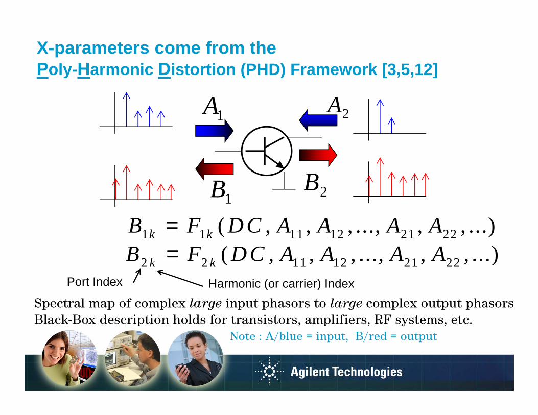
X-parameters come from thePoly -Harmonic Distortion (PHD) Framework [3,5,12]Poly -Harmonic Distortion (PHD) Framework [3,5,12]
2A1A
B B
1 1 11 12 21 22( , , , ..., , , ...)k kB F D C A A A A=1B 2B
1 1 11 12 21 22( , , , ..., , , ...)k kB F D C A A A A=2 2 11 12 21 22( , , , ..., , , ...)k kB F D C A A A A=
Port Index Harmonic (or carrier) IndexPort Index Harmonic (or carrier) Index
Spectral map of complex large input phasors to large complex output phasors
Black-Box description holds for transistors, amplifiers, RF systems, etc.
Note : A/blue = input, B/red = outputNote : A/blue = input, B/red = output
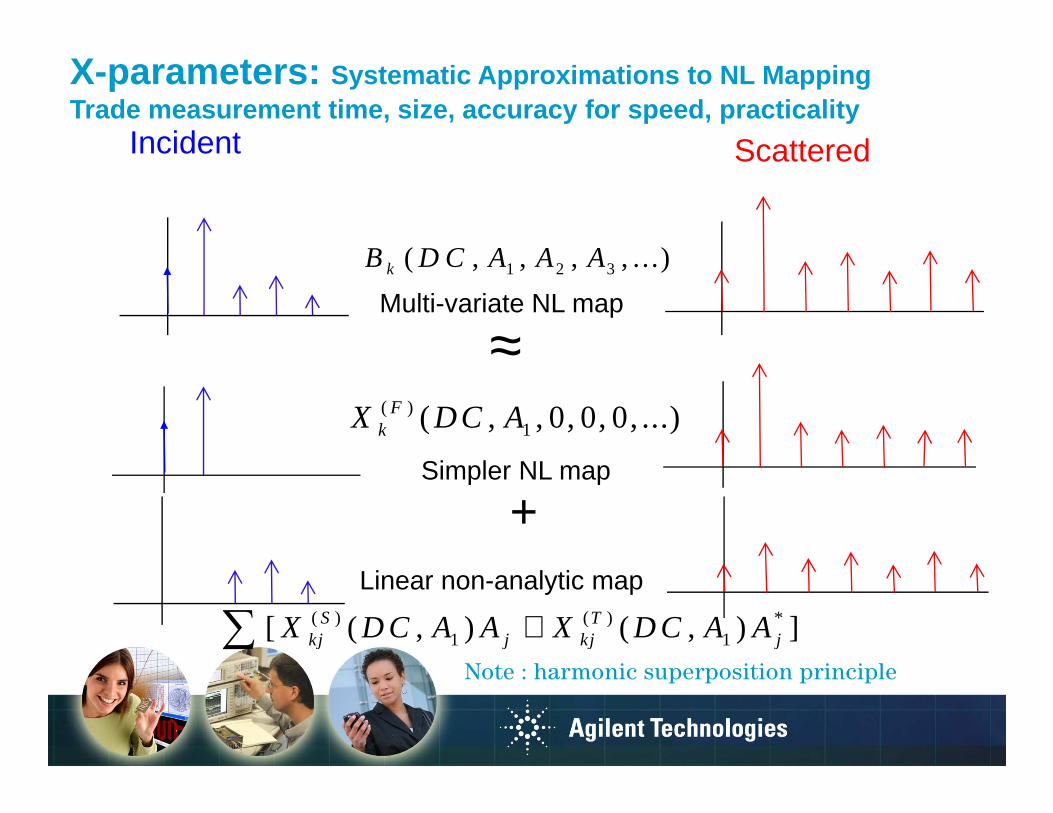
X-parameters: Systematic Approximations to NL MappingTrade measurement time, size, accuracy for speed, p racticality
Incident ScatteredIncident Scattered
( , , , , ...)B D C A A A
Multi-variate NL map1 2 3( , , , , ...)kB D C A A A
≈
Simpler NL map
( )1( , , 0, 0, 0, ...)F
kX DC A
≈
+Simpler NL map
Linear non-analytic map( ) ( ) *
1 1[ ( , ) ( , ) ]S Tkj j kj jX D C A A X D C A A+∑
Note : harmonic superposition principle Note : harmonic superposition principle

X-Parameter Experiment Design & IdentificationIdeal Experiment DesignIdeal Experiment Design
E.g. functions for Bpm (port p, harmonic m)
( ) ( ) ( ) *11 , 11 , 11( ) ( ) ( )F m S m n T m n
pm pm pm qn qn pm qn qnB X A P X A P A X A P A− += + +
Perform 3 independent experiments with fixed A11 using orthogonal phases of A21
input Aqn output Bpm
( ) ( ) ( )(1) ( ) ( ) (1) ( ) (1)*11 , 11 , 11
F m S m n T m npm pm pm qn qn pm qn qnB X A P X A P A X A P A− += + +
input Aqn output Bpm
ImIm( )(0) ( )
11F m
pm pmB X A P=
( ) ( ) ( )11 , 11 , 11pm pm pm qn qn pm qn qnB X A P X A P A X A P A= + +
( ) ( ) ( )(2) ( ) ( ) (2) ( ) (2)*11 , 11 , 11
F m S m n T m npm pm pm qn qn pm qn qnB X A P X A P A X A P A− += + +
Re
Re
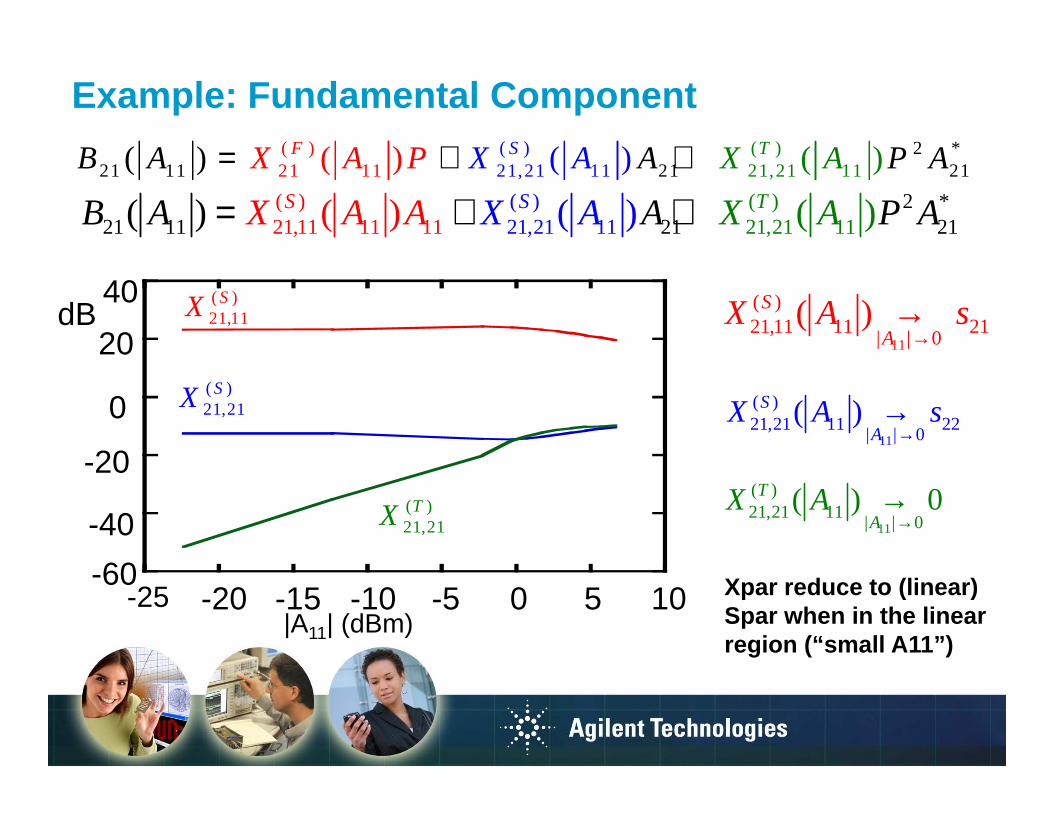
Example: Fundamental Component( )( ) ( ) 2 *()( ) ( )( ) TF SXB AA A PAP X X A A= + +( )( )
21 11( )21,21
2 *21 11 21 2121 11,21 11()( ) ( )( ) TF SXB AA A PAP X X A A= + +
( )21,21
( )( )21,11 11 1
2 *21 1 21,21 11 111 121 21(( ( )) ) () TSSB X A X AA A PA X A A= + +
11
( )21,11 11 21
| | 0( ) S
AX A s
→→40
20dB
( )21,11
SX20
0
-20
( )21,21
SX11
( )21,21 11 22
| | 0( )S
AX A s
→→
11
( )21,21 11
| | 0( ) 0T
AX A
→→
-60
-40
-20( )21,21
TX
-60-25 -20 -15 -10 -5 0 5 10
|A11| (dBm)Xpar reduce to (linear) Spar when in the linear region (“small A11”)
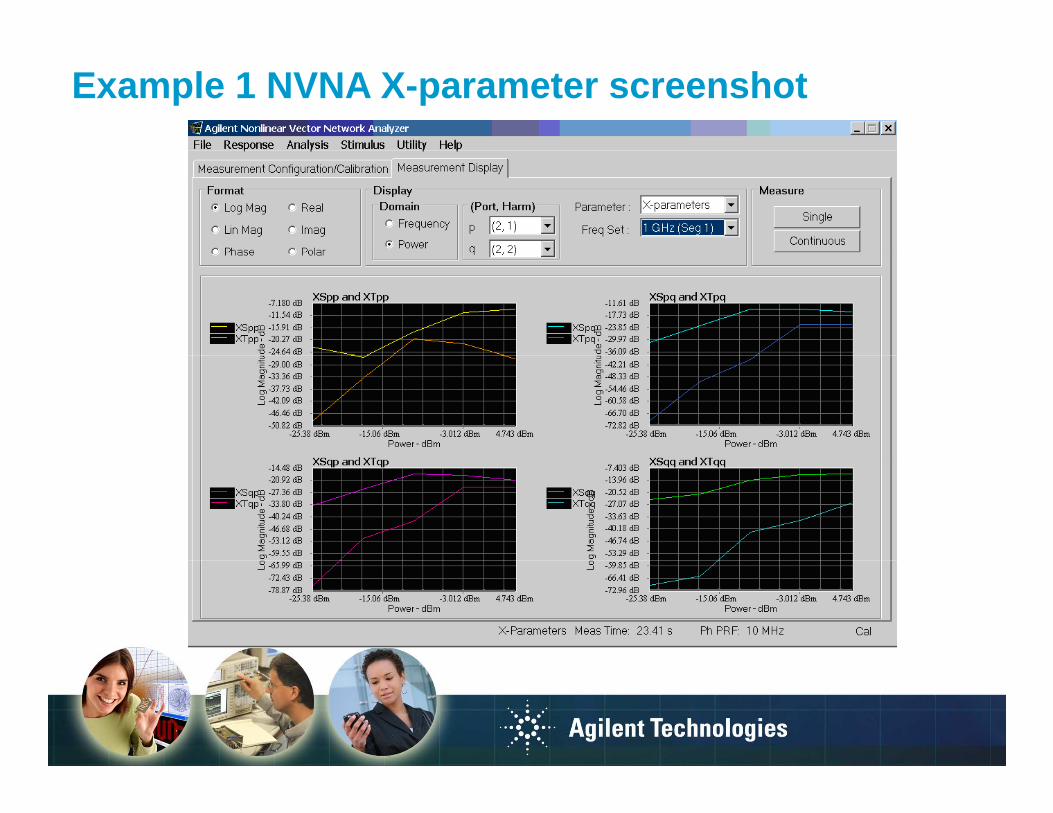
Example 1 NVNA X-parameter screenshot

Example 2 NVNA X-parameter screenshot

X-parameter Application Flow
Automated DUT X-params measured on NVNAAutomated DUT X-params measured on NVNA
Application creates data-specific instance Simulator
PHD instancesCompiled PHD Component simulates using data
MDIF File
NVNA v2v1
ConnectorX1
MCA_ZX60_2522MCA_ZX60_2522_1fundamental_1=fundamental
MCA_ZFL_11ADMCA_ZFL_11AD_1fundamental_1=fundamental
RR1R=25 Ohm
V_1ToneSRC14
Freq=fundamentalV=polar(2*A11N,0) V
RR11R=50 Ohm DC_Block
DC_Block1DC_BlockDC_Block2
I_Probei2
I_Probei1
PHD instances
Data-specific File Data-specific simulatable instance
Compiled PHD component
Harmonic Bal:
DUTΦ Ref
5
10
15
20
25
.
71
72
73
74
75
76
.
Simulation and Design
Harmonic Bal:magnitude & phase of harmonics, frequency dep. and mismatch
Measure X-Parameters -28 -26 -24 -22 -20 -18 -16 -14 -12 -10 -8 -6-30 -4
-30
-20
-10
0
-40
10
.
.
-28 -26 -24 -22 -20 -18 -16 -14 -12 -10 -8 -6-30 -4
-60
-50
-40
-30
-20
-10
0
-70
10
.
.
-28 -26 -24 -22 -20 -18 -16 -14 -12 -10 -8 -6-30 -4
5
0
.
-28 -26 -24 -22 -20 -18 -16 -14 -12 -10 -8 -6-30 -4
70
69
.
-28 -26 -24 -22 -20 -18 -16 -14 -12 -10 -8 -6-30 -4
-135
-130
-125
-120
-140
-115
-28 -26 -24 -22 -20 -18 -16 -14 -12 -10 -8 -6-30 -4
0
2
4
6
8
10
12
-2
14
.
.
-10 -5 0 5 10 15-15 20
-30
-20
-10
0
10
-40
20
.
.
Envelope:Accurately simulate NB multi-tone or complex stimulus
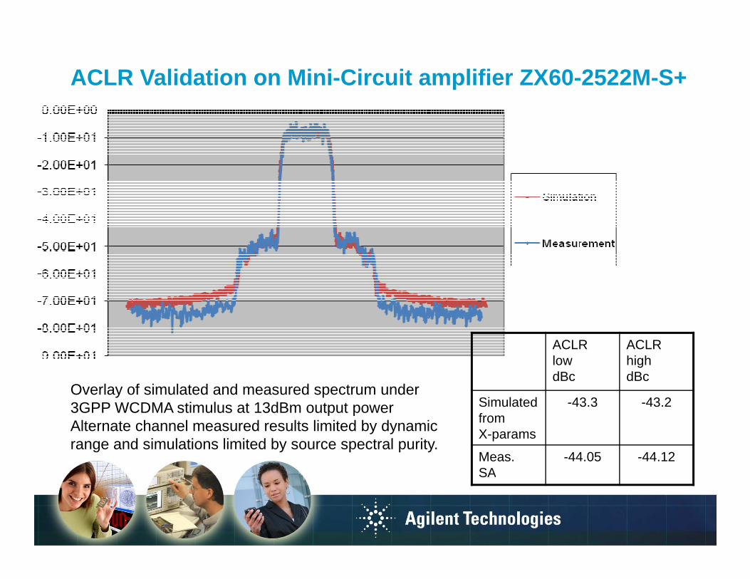
ACLR Validation on Mini-Circuit amplifier ZX60-2522 M-S+
Overlay of simulated and measured spectrum under 3GPP WCDMA stimulus at 13dBm output power
ACLR lowdBc
ACLR highdBc
Simulated -43.3 -43.23GPP WCDMA stimulus at 13dBm output powerAlternate channel measured results limited by dynamic range and simulations limited by source spectral purity.
Simulated fromX-params
-43.3 -43.2
Meas. SA
-44.05 -44.12SA

Measurement-based nonlinear design with X-parameter s
ZFL-AD11+11dB gain, 3dBmmax output power
SourceConnector
80 psdelay
ZX60-2522M-S+23.5dB gain, 18dBm
max output powerLoad
v2v1
ConnectorX1
MCA_ZX60_2522MCA_ZX60_2522_1fundamental_1=fundamental
MCA_ZFL_11ADMCA_ZFL_11AD_1fundamental_1=fundamental
RR1R=25 Ohm
RR11R=50 Ohm DC_Block
DC_Block1DC_BlockDC_Block2
I_Probei2
I_Probei1
fundamental_1=fundamentalfundamental_1=fundamental
V_1ToneSRC14
Freq=fundamentalV=polar(2*A11N,0) V Amplifier Component Models from individual X-parameter measurements

Results
Cascaded S
imulation vs. M
easurement
Cascaded S
imulation vs. M
easurement
Red: C
ascade Measurem
entB
lue: Cascaded X
-parameter S
imulation
Light Green: C
ascaded Sim
ulation, No X
(T)term
sLight G
reen: Cascaded S
imulation, N
o X(T
)terms
Dark G
reen: Cascaded M
odels, No X
(S)or X
(T)term
s
34 36
dB(b2ref[::,1]/a1ref[::,1])dB(b2NoT[::,1]/a1NoT[::,1])
dB(b2NoST[::,1]/a1NoST[::,1])
Fundam
ental Gain
74 76
unwrap(phase(b2[::,1]))unwrap(phase(b2ref[::,1]))
unwrap(phase(b2NoT[::,1]))unwrap(phase(b2NoST[::,1]))
Fundam
ental Phase
30 32 34
dB(b2[::,1]/a1[::,1])dB(b2ref[::,1]/a1ref[::,1])
dB(b2NoT[::,1]/a1NoT[::,1])dB(b2NoST[::,1]/a1NoST[::,1])
70 72 74
unwrap(phase(b2[::,1]))unwrap(phase(b2ref[::,1]))
unwrap(phase(b2NoT[::,1]))unwrap(phase(b2NoST[::,1]))
-28-2
6-24
-22-20
-18-16
-14
-12-10
-8-6
-30-4
2826
Pinc
dB(b2ref[::,1]/a1ref[::,1])dB(b2NoT[::,1]/a1NoT[::,1])
dB(b2NoST[::,1]/a1NoST[::,1])
-28-26
-24-22
-20-18
-16
-14-12
-10-8
-6-3
0-4
6866
Pinc
unwrap(phase(b2[::,1]))
Pincref
unwrap(phase(b2ref[::,1]))unwrap(phase(b2NoT[::,1]))
unwrap(phase(b2NoST[::,1]))
Pincref

Results
Cascaded S
imulation vs. M
easurement
Cascaded S
imulation vs. M
easurement
Red: C
ascade Measurem
entB
lue: Cascaded X
-parameter S
imulation
Light Green: C
ascaded Sim
ulation, No X
(T)term
sLight G
reen: Cascaded S
imulation, N
o Xterm
sD
ark Green: C
ascaded Models, N
o X(S
)or X(T
)terms
Fundam
ental % E
rrorS
econd Harm
onic % E
rror
(b2[::,2]-b2ref[::,2])/b2ref[::,2]*100(b2NoT[::,2]-b2ref[::,2])/b2ref[::,2]*100
(b2NoST[::,2]-b2ref[::,2])/b2ref[::,2]*100
6 8
10 12
(b2[::,1]-b2ref[::,1])/b2ref[::,1]*100(b2NoT[::,1]-b2ref[::,1])/b2ref[::,1]*100
(b2NoST[::,1]-b2ref[::,1])/b2ref[::,1]*100
60 80
100
(b2[::,2]-b2ref[::,2])/b2ref[::,2]*100(b2NoT[::,2]-b2ref[::,2])/b2ref[::,2]*100
(b2NoST[::,2]-b2ref[::,2])/b2ref[::,2]*100
-28-26
-24-22
-20-18
-16-14
-12-10
-8-6
-30-4
2 4 60
(b2[::,1]-b2ref[::,1])/b2ref[::,1]*100(b2NoT[::,1]-b2ref[::,1])/b2ref[::,1]*100
(b2NoST[::,1]-b2ref[::,1])/b2ref[::,1]*100
-28-26
-24
-22
-20
-18
-16
-14-12
-10-8
-6-30
-4
20 400(b2[::,2]-b2ref[::,2])/b2ref[::,2]*100
(b2NoT[::,2]-b2ref[::,2])/b2ref[::,2]*100(b2NoST[::,2]-b2ref[::,2])/b2ref[::,2]*100
-28-26
-24-22
-20-18
-16-14
-12-10
-8-6
-30-4
Pinc
-28-26
-24
-22
-20
-18
-16
-14-12
-10-8
-6-30
-4
Pinc
“X-param
eters enable predictive nonlinear design from N
L data”

Summary• X-parameters are a mathematically correct superset of S-• X-parameters are a mathematically correct superset of S-
parameters for nonlinear devices under large-signal conditions– Rigorously derived from general PHD theory; flexible, practical, powerful
• X-parameters can be accurately measured by automated set • X-parameters can be accurately measured by automated set of experiments on the new Agilent NVNA instrument
• Together with the PHD component, measured X-parameters • Together with the PHD component, measured X-parameters can be used in ADS to design nonlinear circuits
• All pieces of the puzzle are available and they fit together!
Nonlinear Measurements
NonlinearSimulation
CustomerApplications
Nonlinear Modeling

Configuration Details
DescriptionN5242A - 400 10 MHz to 26.5 GHz 4-port
Opt 419: 4-port attenuators & bias tees Opt 419: 4-port attenuators & bias tees
Opt 423: Source switching & combining network
Opt 080: Frequency Offset Mode
Opt 510: Nonlinear component characterization measurements(requires 400,419,080)
Opt 514: Nonlinear X-parameters (requires 423, opt 510 & ext. source)
Opt 518: Nonlinear pulse envelope domainOpt 518: Nonlinear pulse envelope domain(requires opt 510,021,025)
Accessories:U9391C Phase reference (2 units required)U9391C Phase reference (2 units required)Power meter & sensor or USB power sensor3.5mm calibration standardsExternal source for X-parameters

PNA Applications Antenna T/R Module
Mm-waveAmplifier Test Pulsed RFAntenna
TestT/R Module
TestMm-wave
Single Connection:Gain compression,
IMD, noise figure, harmonics,
true differential,
PAE, hot S
Amplifier Test Pulsed RF
and DC
325 GHz325 GHzPNA-LPNA-L500 GHz500 GHz
PAE, hot S22
Materials Measurements
50 GHz50 GHz67 GHz67 GHz110 GHz110 GHz325 GHz325 GHz
PNA-L
PNA
PNA-X
PNA-L
PNA
PNA-X
500 GHz500 GHz
Mixer Test
NVNA
13.5 GHz13.5 GHz20 GHz20 GHz40 GHz40 GHz50 GHz50 GHz67 GHz67 GHz
Load Pull
Noise Parameters Signal Integrity
Component Characterization
X-Parameter Extraction
Pulse Envelope Domain
www.agilent.com/find/pna
6 GHz6 GHz13.5 GHz13.5 GHz
Scanning MicroscopeMicroscope
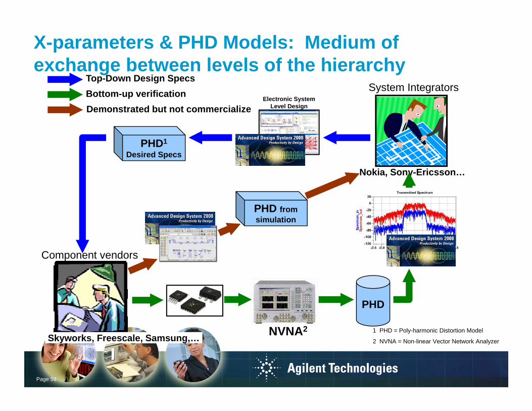
X-parameters & PHD Models: Medium of exchange between levels of the hierarchy
Top-Down Design SpecsTop-Down Design Specs
Demonstrated but not commercialize
Bottom-up verification
ESL
Electronic System Level Design
System Integrators
Nokia, Sony-Ericsson…
PHD1
Desired Specs
PHD fromsimulation
Component vendors
Skyworks, Freescale, Samsung,…NVNA2
PHD
1 PHD = Poly-harmonic Distortion Model
Page 59
Skyworks, Freescale, Samsung,…NVNA
2 NVNA = Non-linear Vector Network Analyzer
References[1] J. Wood, D. E. Root, N. B. Tufillaro, “A behavioral modeling
approach to nonlinear model-order reduction for [8] D. E. Root, D. Sharrit, J. Verspecht, “Nonlinear Behavioral
Models with Memory: Formulation, Identification, and approach to nonlinear model-order reduction for RF/microwave ICs and systems,” IEEE Transactions on Microwave Theory and Techniques, Vol. 52, Issue 9, Part 2, Sept. 2004 pp. 2274-2284
[2] Agilent HMMC-5200 DC-20 GHz HBT Series-Shunt Amplifier, Data Sheet, August 2002.
Models with Memory: Formulation, Identification, and Implementation,” 2006 IEEE MTT-S International Microwave Symposium Workshop (WSL) on Memory Effects in Power Amplifiers
[9] Blockley et al 2005 IEEE MTT-S International Microwave Symposium Digest, Long Beach, CA, USA, June 2005.
[3] J. Verspecht, M. Vanden Bossche, F. Verbeyst, “Characterizing Components under Large Signal Excitation: Defining Sensible `Large Signal S-Parameters'?!,” in 49th IEEE ARFTG Conference Dig., Denver, CO, USA, June 1997, pp. 109-117.
[4] J. Verspecht, D.E. Root, J. Wood, A. Cognata, “Broad-Band,
[10] Jan Verspecht Patent US 7,038,468 B2 (issued May 2, 2006 based on a provisional patent 60/477,349 filed on June 11, 2003)
[11] Soury et al 2005 IEEE International Microwave Symposium Digest pp. 975-978
[4] J. Verspecht, D.E. Root, J. Wood, A. Cognata, “Broad-Band, Multi-Harmonic Frequency Domain Behavioral Models from Automated Large-Signal Vectorial Network Measurements,” in 2005 IEEE MTT-S International Microwave Symposium Digest, Long Beach, CA, USA, June 2005.
[5] D. E. Root, J. Verspecht, D. Sharrit, J. Wood, and A. Cognata, “Broad-Band Poly-Harmonic Distortion (PHD)
[12] J. Verspecht and D. E. Root, “Poly-Harmonic Distortion Modeling,” in IEEE Microwave Theory and Techniques Microwave Magazine, June, 2006.
[13] J. Verspecht, D. Gunyan, J. Horn, J. Xu, A. Cognata, and D.E. Root, “Multi-tone, Multi-Port, and Dynamic Memory Enhancements to Cognata, “Broad-Band Poly-Harmonic Distortion (PHD)
Behavioral Models from Fast Automated Simulations and Large-Signal Vectorial Network Measurements”, IEEE Transactions on Microwave Theory and Techniques Vol. 53. No. 11, November, 2005 pp. 3656-3664
[6] J. Wood, D. E. Root, editors, Fundamentals of NonlinearBehavioral Modeling for RF and Microwave Design , 1st
“Multi-tone, Multi-Port, and Dynamic Memory Enhancements to PHD Nonlinear Behavioral Models from Large-Signal Measurements and Simulations,” 2007 IEEE MTT-S Int. Microwave Symp. Dig.,Honolulu, HI, USA, June 2007.
[14] Horn et al 2008 Power Amplifier Symposium, Orlando, Jan. 2008
[15] Horn et al 2008 IEEE European Microwave Conference, Behavioral Modeling for RF and Microwave Design , 1sted. Norwood, MA, USA, Artech House, 2005.
[7] Root et al US Patent # 7295961 2007
[15] Horn et al 2008 IEEE European Microwave Conference, Amsterdam, October, 2008
[16] Simpson et al to be published in 2008 IEEE ARFTG Conference, Portland, OR December, 2008

Return Loss
Hierarchical NL Design using meas. X-params in ADS: Measured System vs Simulation: Fundamental
GainMagnitude
Return Loss
Magnitude
Blue: PHD Hierarchical ModelRed: Measurements
Magnitude
Blue: PHD Hierarchical ModelRed: Measurements
Phase Phase

Hierarchical NL Design using meas. X-params in ADS: Measured System vs Simulation: 2 nd Harmonic
B2 B1
Magnitude Magnitude
B2 B1
Blue: PHD Hierarchical ModelRed: Measurements
Magnitude
Blue: PHD Hierarchical ModelRed: Measurements
Phase Phase

Hierarchical NL Design using meas. X-params in ADS: Measured System vs Simulation: 3 rd Harmonic
B2 B1
Magnitude Magnitude
B2 B1
Blue: PHD Hierarchical ModelRed: Measurements
Magnitude
PhasePhase
Blue: PHD Hierarchical ModelRed: Measurements

Load-Dependent Measured X-parameters [16]

PHD Model Offers:
Straight forward setup and calibration• A setup and calibration that is only slightly more complex than a regular VNA measurement.Anticipate the behavior of the device under a large set of operating conditions by Anticipate the behavior of the device under a large set of operating conditions by sweeping bias points, frequencies, loads, power, all automatically
Fast characterization • <30 seconds for one bias point and frequency – fund + 2 harmonics).• <30 seconds for one bias point and frequency – fund + 2 harmonics).• Weeks to months using traditional methods
(In fact using the old method with Load Pull using passive tuners, one bias point takes about 30 minutes, at the fundamental only. Characterizing using harmonic load pull would take days to weeks. Old methods give no model nor phase (waveform) info.)
A PHD behavioral model is available almost directly after the measurement.A PHD behavioral model is available almost directly after the measurement.• based on X-parameters that gives nonlinear information about the PA, and its harmonicsEstimate and predict parameters previously not poss ible to simulate• Having a NL model allows for Harmonic Balance and envelope simulations with modulated • Having a NL model allows for Harmonic Balance and envelope simulations with modulated
sources. We can estimate and predict many parameters that were previously not possible to simulate. PhErr, EVM, ACLR, Mod Spectrum