nonlinear wind analysis of single-doppler radar
TRANSCRIPT

Nonlinear Wind Analysis of Single-Doppler Radar Observations within a DVADFramework
XIAOWEN TANG
Key Laboratory for Mesoscale Severe Weather/Ministry of Education, and School of Atmospheric Sciences,
Nanjing University, Nanjing, China
WEN-CHAU LEE
National Center for Atmospheric Research,* Boulder, Colorado
YUAN WANG
Key Laboratory for Mesoscale Severe Weather/Ministry of Education, and School of Atmospheric Sciences,
Nanjing University, Nanjing, China
(Manuscript received 25 July 2014, in final form 2 April 2015)
ABSTRACT
The application of the distance velocity azimuth display (DVAD) method to the retrieval of vertical wind
profiles from single-Doppler radar observations is presented in this study. It was shown that Doppler velocity
observations at a constant altitude can be expressed as a single polynomial function for both linear and
nonlinear wind fields in DVAD. Only a one-step least squares fitting of a polynomial function is required to
obtain the vertical wind profile of a real wind field. The mathematic formulation of DVAD results in two
advantages over the traditional nonlinear VAD method used for the nonlinear analysis of single-Doppler
observations. First, the requirement of only one-step least squares fitting leads to robust performance when
Doppler velocity observations are contaminated by unevenly distributed data noise and voids. Second, the
degree of nonlinearity to properly represent a real wind field can be directly estimated in DVAD instead of
being empirically determined in the traditional method. A proper nonlinear wind model for approximating
the real wind field can be objectively derived using theDVADmethod. Themerits ofDVADas a quantitative
single-Doppler analysis method were compared with the traditional method using both idealized and real
datasets. Results show that the simplicity and robust performance of DVAD make it a good candidate for
single-Doppler retrieval in operational use.
1. Introduction
The ground-based weather Doppler radar has been an
important observational tool for deducing kinematic
structures of precipitating (Browning and Wexler 1968;
Waldteufel and Cobin 1979; Lee et al. 1994), and more
recently nonprecipitating (Kollias et al. 2001; Bluestein
et al. 2004), cloud systems. The ability to observe a large
region with higher spatial and temporal resolutions than
those obtained from the rawinsonde and surface station
measurements has greatly advanced our understanding of
various mesoscale and convective weather systems
(Houze 2004). Despite its wide applications in both re-
search and operational communities, the direct in-
terpretation of the three components (u, y, w) of a wind
field from the observed Doppler velocity is not straight-
forward because a Doppler radar only measures the
component of awind field projected along the radar beam
direction. The retrieval of basic physical properties
(horizontal velocity, vertical velocity, divergence, de-
formation, and vorticity) from single-Doppler radar ob-
servations can only be accomplished with certain
assumptions on the structure of the actual wind field.
Previous studies have used a linear assumption (e.g.,
* The National Center for Atmospheric Research is sponsored
by the National Science Foundation.
Corresponding author address: Yuan Wang, Key Laboratory for
Mesoscale Severe Weather/Ministry of Education, and School of
Atmospheric Sciences, Nanjing University, Nanjing, China.
E-mail: [email protected]
1538 JOURNAL OF APPL IED METEOROLOGY AND CL IMATOLOGY VOLUME 54
DOI: 10.1175/JAMC-D-14-0194.1
� 2015 American Meteorological Society
Lhermitte and Atlas 1961; Browning and Wexler 1968;
Waldteufel and Cobin 1979; Srivastava and Matejka
1986; Matejka and Srivastava 1991), circular vortex as-
sumption (Lee et al. 1994, 1999), and steady assumption
(Peace et al. 1969; Bluestein and Hazen 1989) to model
and retrieve the physical parameters of a real wind field
observed by a single-Doppler radar. Except for these
Doppler velocity-based algorithms, the horizontal wind
vectors have also been deduced by tracking radar re-
flectivity patterns (Rinehart and Garvey 1978; Tuttle and
Foote 1990; Tuttle and Gall 1999). These studies signifi-
cantly advanced the utilization of single-Doppler radar
observations to estimate key characteristics of atmo-
spheric kinematic structure.
Doppler velocity can be expressed in analytic functions
on the aforementioned simplified wind fields. Limited
physical information of these real simplified wind fields
can be obtained by conducting a least squares fitting
(LSF) of the observations to the analytic functions. The
VAD method (Browning and Wexler 1968) expressed
Doppler velocities along ‘‘a ring of constant radius cen-
tered at the radar site’’ (hereinafter referred to as a VAD
ring) as a Fourier series, a function of azimuth angle. If
the wind field is linear, the resulting Fourier coefficients
of the LSF can be physically interpreted as the mean di-
vergence, mean horizontal winds, and mean horizontal
deformation averaged over an area encircled by the
VAD ring. By processing the data of multiple VAD rings
on different radii and/or different elevation angles, the
VAD vertical wind profile1 (e.g., Fig. 1 in Chrisman and
Smith 2009) can be deduced and has been widely used in
both research and operations (e.g., Davis and Lee 2012;
Giammanco et al. 2013; Kingsmill et al. 2013).
The spatial linearity is the fundamental assumption
for deducing physical parameters (i.e., the Fourier co-
efficients) of a wind field from the VAD analysis.
However, the departure of actual wind fields from lin-
earity is common in real weather situations (Rabin and
Zawadzki 1984). When nonlinear2 wind components
exist, the Fourier coefficients deduced in the VAD
analysis are not representative of the mean kinematic
properties in a real wind field (Waldteufel and Cobin
1979; Koscielny et al. 1982; Caya and Zawadzki 1992).
Unresolved nonlinear wind components could contam-
inate the retrieval of linear wind components
(Waldteufel and Cobin 1979; Koscielny et al. 1982) and
lead to significant errors in retrieved vertical wind pro-
files (VWPs). In their formulation of the extended VAD
(EVAD) method, Matejka and Srivastava (1991) also
noticed the necessity to include certain nonlinear wind
components to retrieve the mean divergence within a
VAD ring. Although real wind fields may not deviate
significantly from a linear distribution under certain
weather conditions, the intrinsic linear wind hypothesis
in the VAD analysis is unduly restrictive in obtaining
accurate kinematic properties for both research and
operational purposes (Caya and Zawadzki 1992, here-
inafter CZ92). Despite the documented detrimental ef-
fect of unresolved nonlinear wind components on VAD
analysis, there is no simple way to examine whether the
wind field is linear. Hence, the existence of nonlinear
wind components was mainly neglected in the VAD
analysis in practice.
CZ92 extensively examined the relationship between
the physical parameters of a nonlinear wind field and the
Fourier coefficients from the VAD analysis. It was
shown that the Fourier coefficients (e.g., Browning and
Wexler 1968) no longer represent those aforementioned
kinematic properties for nonlinear wind fields, except
for the divergence term. However, the Fourier co-
efficients become functions of radius at a constant alti-
tude in nonlinear wind fields. By utilizing this range
dependence, a second polynomial fit was used to re-
trieve the horizontal wind vector at the radar site for
nonlinear wind fields. The work presented in CZ92 not
only clarified the relations between the physical pa-
rameters of a wind field and the results of VAD analysis
under nonlinear conditions, but also proposed a new
method (hereinafter referred to as NVAD) to account
for the nonlinearity and obtain physically meaningful
results. However, CZ92 only tested the NVAD method
in limited cases in which its practical limitations were not
fully explored.
Mesoscale weather systems typically contain non-
linear winds. During the Southwest Monsoon Experi-
ment (SoWMEX) and the Terrain-Influenced Monsoon
Rainfall Experiment (TiMREX) field campaign (Jou
et al. 2011), the NVAD method was implemented to
deduce more frequent and accurate VWPs from
Doppler velocity observations collected by the National
Center for Atmospheric Research (NCAR) S-band
dual-polarization Doppler radar (S-Pol) to supplement
1 The VAD vertical wind profile is commonly abbreviated as
VWP in operational radar product catalogs. The same abbreviation
is also used for the vertical wind profile, and logically the VAD
wind profile is just one particular vertical wind profile calculated by
theVADmethod. Since the vertical wind profiles referred to in this
study are not computed by the original VAD method, the abbre-
viation VWP is saved in later parts of this paper to refer to its
original meaning, ‘‘vertical wind profile.’’2 The word ‘‘nonlinear’’ is a common nomenclature meaning any
variation in time and/or space that is not constant. Since this paper
is focusing on the retrieval of horizontal winds at different alti-
tudes, here nonlinear means higher-order variations of winds in a
plane, or simply the nonuniformity in theX–Y plane of a Cartesian
coordinate system.
JULY 2015 TANG ET AL . 1539
the rawinsonde VWPs, which were collected 4–8 times
per day. After processing a large set of SoWMEX/
TiMREX data, it was found that the NVAD method
generated inconsistent VWPs in many circumstances.
The NVAD method is sensitive to the distribution of
data noise and voids in the Doppler velocity observa-
tions. The sensitivity is again related to the mathemati-
cal formulation and corresponding computation process
used in NVAD.
The purpose of this study is to propose an alternative
method, the distance velocity azimuth display (DVAD;
Lee et al. 2014), to deduceVWPs in nonlinear wind fields.
Instead of using Doppler velocity Vd alone to analyze
nonlinear wind fields observed by a single-Doppler radar,
the DVAD method uses the quantity rVd (Vd scaled by
the distance from the radar to the gate, r) as a variable. A
description of the general use of rVd to analyze single-
Doppler radar observations can be found in Lee et al.
(2014). In the DVAD method, the linear wind field is
represented exclusively by a bivariate quadratic equation
representing three basic types of conic sections in a
Cartesian coordinate system. Nonlinear wind fields can
be expressed in the samemathematical form with higher-
order3 equations. In addition to its graphical intuition and
mathematical conciseness, the potential of using DVAD
to quantitatively retrieve physical parameters from both
linear and nonlinear wind fields is exploited in this study,
and the results are compared with the VWPs deduced
from the NVAD method. It is shown that DVAD is
consistent with NVAD under idealized conditions but is
more robust when processing real observations. The
concise mathematical expression of DVAD allows the
estimation of the degree of nonlinearity of real wind fields
in an objective way.
The rest of this paper is organized as follows. In section
2, a brief review of the mathematical formulation of
NVAD and DVAD is provided. In section 3, an evalua-
tion of VWPs retrieved from NVAD and DVAD using
an idealized dataset is conducted, and the potential lim-
itations of NVAD are discussed. In section 4, field cam-
paign and operational Next Generation Weather Radar
(NEXRAD) datasets are used to demonstrate the robust
performance of DVAD. In section 5, an objective way of
assessing the nonlinearity of actual wind fields is dis-
cussed. Discussion and conclusions are given in section 6.
2. Review of NVAD and DVAD
a. NVAD
Common volume scans of ground-based Doppler ra-
dars can be viewed as data collected on a series of con-
ical surfaces with different elevation angles. The
Doppler velocity Vd at a point P(x, y, z) centered at the
radar can be expressed in terms of Cartesian velocities
(u, y, and w), terminal fall speed yt, azimuth angle a,
elevation angle b, and the slant range r, as illustrated in
Armijo (1969):
Vd5 ux
r1 y
y
r1 (w1 yt)
z
r
5 u sina cosb1 y cosa cosb1 (w1 yt) sinb . (1)
The horizontal components u and y of a linear wind field
can be expressed using their Taylor expansions at a plane
of constant altitude by neglecting the vertical velocity w
and terminal fall speed of precipitation particles yt as
u5 u01 uxx1 uyy and
y5 y01 yxx1 yyy . (2)
Here, u0 and y0 are the constant horizontal wind at the
radar site, and ux, uy, yx, and yy are the first derivatives of
the horizontal winds. By substituting (2) into (1), Vd can
be written as (assuming b5 0)
Vd(a)5r
2(ux1 yy)1 u0 sina1 y0 cosa
1r
2(uy1 yx) sin2a1
r
2(yy2 ux) cos2a . (3)
Fitting Vd as a harmonic function of azimuth a at a fixed
range r, the coefficients of (3) are related to the mean
values of kinematic parameters of the real wind field
within a VAD ring as
a05r
2(ux1 yy), a15 u0, b1 5 y0,
a25r
2(uy1 yx), and b2 5
r
2(yy2 ux) , (4)
where a1 and b1 equal the mean horizontal wind and a0,
a2, and b2 equal the mean divergence, stretching, and
shearing deformation scaled by a factor of r/2, re-
spectively (Browning and Wexler 1968). The equations
in (4) are the basis for interpreting the results of the
3 There will be three sets of equations characterized by their
‘‘orders’’ in this paper. The order of a wind model means the
highest order in a truncated Taylor series used to approximate the
real wind field. The order of VAD analysis means the highest order
of a truncated Fourier series used to model the observed Doppler
velocities. Since single-Doppler analysis methods are always based
on a prescribed wind model, a VAD analysis with order n1 1
corresponds to a wind model with order n (Caya and Zawadzki
1992). The order of DVAD analysis means the highest order of a
two-dimensional polynomial function, which is also one order
higher than the corresponding wind model.
1540 JOURNAL OF APPL IED METEOROLOGY AND CL IMATOLOGY VOLUME 54
traditional VAD analysis and are only strictly valid
under a linear wind assumption. CZ92 extends the tra-
ditional VAD analysis by adding nonlinear terms (to
keep the expression simple, only nonlinear terms up to
third order are included) into (2). Then, Vd is expressed
in the following form:
Vd 5r
2
�ux1 yy1
1
8uxxxr
211
8uxyyr
211
8yxxyr
211
8yyyyr
2
�
1
�u01
3
8uxxr
211
8uyyr
211
4yxyr
2
�sina
1
�y01
1
4uxyr
211
8yxxr
213
8yyyr
2
�cosa
1r
2
�uy1 yx1
1
4uxxyr
211
12uyyyr
211
12yxxxr
211
4yxyyr
2
�sin2a
1r
2
�yy2 ux2
1
6uxxxr
211
6yyyyr
2
�cos2a
1
�21
8uxxr
2 11
8uyyr
2 11
4yxyr
2
�sin3a
1
�21
8yxxr
211
8yyyr
221
4uxyr
2
�cos3a
1
�2
1
16uxxyr
3 11
48uyyyr
3 21
48yxxxr
311
16yxyyr
3
�sin4a
1
�1
48uxxxr
3 21
16uxyyr
3 21
16yxxyr
311
48yyyyr
3
�cos4a1⋯ , (5)
where the subscripts x, y of variables u, y stand
for the partial derivatives of the horizontal winds
(e.g., uxyy is equal to ›3u/›x›2y). After adding
nonlinear terms, the relations between Fourier co-
efficients and kinematic parameters of a wind field
become
a0 5r
2
�ux1 yy 1
1
8uxxxr
211
8uxyyr
211
8yxxyr
211
8yyyyr
2
�,
a1 5 u013
8uxxr
211
8uyyr
211
4yxyr
2, b15 y011
4uxyr
211
8yxxr
213
8yyyr
2,
a2 5r
2
�uy1 yx 1
1
4uxxyr
211
12uyyyr
211
12yxxxr
211
4yxyyr
2
�, and
b2 5r
2
�yy2 ux 2
1
6uxxxr
211
6yyyyr
2
�. (6)
Meanwhile, the mean kinematic quantities for a third-
order nonlinear wind field can be derived by expanding
(2) and integrating with respect to azimuth a from 0 to
2p as follows:
(ux1 yy)mean5 ux 1 yy11
8uxxxr
211
8uxyyr
2 11
8yyyyr
211
8yxxyr
2,
umean5 u0 11
8uxxr
2 11
8uyyr
2,
ymean5 y011
8yxxr
211
8yyyr
2, and
(uy1 yx)mean5 uy 1 yx11
8uxxyr
211
8uyyyr
2 11
8yxxxr
211
8yxyyr
2 . (7)
JULY 2015 TANG ET AL . 1541

Acomparison of terms on the right-hand sides of (6) and
(7) indicates that, except for the mean divergence term,
the physical wind parameters in (7) no longer possess the
same relations to the Fourier coefficients in (6) as in the
linear case shown in (4). The physical wind parameters
cannot be solved by the same VAD technique by fitting
Vr to a higher-order Fourier series along a VAD ring.
Although the mean physical parameters within a VAD
ring cannot be obtained when the wind field is nonlinear,
CZ92 noticed that each of the Fourier coefficients in (6)
is a polynomial function of r. Therefore, these physical
quantities at the radar site (i.e., r 5 0) can be evaluated
by a second LSF via the Fourier coefficients obtained at
different ranges. This two-step LSF procedure that is
based on (6) formed the basis for the NVAD analysis
proposed by CZ92. Plausible VWPs in clear-air bound-
ary layers were retrieved by NVAD (CZ92).
b. DVAD
The DVAD method uses the quantity rVd to analyze
nonlinear wind fields observed by a ground-based
Doppler radar. The detailed mathematical expression
and graphical interpretation of DVAD can be found in
Lee et al. (2014). Here, the mathematical derivation
related to quantitative analysis of DVAD is briefly re-
viewed. By multiplying both sides of (1) by r, the
quantity rVd at a point P(x, y, z) can be written as
rVd 5ux1 yy1 (w1 yt)z , (8)
where the Cartesian coordinates (x, y, and z) are cen-
tered at the radar. The altitude z of a data point is de-
termined using the 4/3 Earth model with a constant
gradient of refractivity (Doviak and Zrnic 2006, 18–23).
The velocity components u, y, and w at a constant alti-
tude can be represented by their Taylor series with re-
spect to the radar site as
u5u01 uxx1 uyy11
2uxxx
2 1 uxyxy11
2uyyy
21 . . . ,
y5 y01 yxx1 yyy11
2yxxx
21 yxyxy11
2yyyy
21 . . . ,
and
w5w0 1wxx1wyy11
2wxxx
21wxyxy11
2wyyy
21 . . . .
(9)
On the spatial scale (;100 km) covered by a Doppler
radar, the mean magnitudes of w and yt are usually one
order smaller than those of u and y. Moreover, the
limited value of the maximum elevation angle (,208)scanned by an operational ground-based Doppler radar
results in a small contribution of w and yt into Vd.
Therefore, both w and yt can be neglected in (8) for the
analysis of operational radar data. Although both w and
yt are neglected in the formulation and computation of
DVAD, this simplification could have potential impact
on the result of DVAD when w and/or yt are large. The
potential impact could be further amplified by the fact
that some research radars have maximum elevation
angles well beyond 208. As a design criterion of DVAD,
it is advised to discard Doppler observations beyond 208elevation angle during computation.
Assuming the horizontal components u and y can be
sufficiently approximated by finite terms of their Taylor
series, then rVd can be rewritten by substituting (9) into
(8) as follows:
rVd 5u0x1 y0y1 uxx21 (uy1 yx)xy
1 yyy21
1
2uxxx
31
�uxy1
1
2yxx
�x2y
1
�1
2uyy 1 yxy
�xy21
1
2yyyy
31 . . . . (10)
It is noted that rVd is a polynomial function of the
Cartesian coordinate x and y without the complexity of
trigonometrical basis functions. Equation (10) can be writ-
ten in a more concise form using the summation notation:
rVd 5 �n
i51�i
j50
cijxi2jy j , (11)
where cij is the coefficient of the two-dimensional (2D)
polynomial function and n is the highest degree of the
2D polynomial function. Assuming there are l Doppler
velocity observations at the same height, the coefficient
cij can be solved for in a least squares sense. For con-
venience of discussion, the least squares–solving process
is represented in vector form:
b5Ac1 � , (12)
where b is a vector with l items each containing observed
rVd,A is an l3mmatrix (l is the number of observations
and m is the total number of coefficients of the poly-
nomial function) depending on the distribution of radar
observations and the order of the nonlinear wind model,
c is a vector containing the coefficients to solve, and � is a
vector representing random error (e.g., noise in the ra-
dar hardware and sampling error) in the observations.
The coefficients contained in c can be solved for by
minimizing the following cost function:
J5 kAc2 bk2 . (13)
Since the basis functions of the polynomial series in (11)
are not intrinsically orthogonal, an algorithm utilizing
1542 JOURNAL OF APPL IED METEOROLOGY AND CL IMATOLOGY VOLUME 54

singular vector decomposition (SVD) is used to solve
the corresponding normal equation of (13) by setting
$J5 0 (Boccippio 1995). In comparing (10) with (11),
the coefficients of the polynomial series are related to
the horizontal components of the wind field at the radar
site as
c10 5 u0 and c115 y0 . (14)
A comparison of (11) and (5) shows that the quantitative
analysis of Doppler radar observations has a concise
mathematical form in DVAD. Linear and nonlinear
wind fields are represented by the same polynomial basis
functions with different orders. As a result, only a one-
step 2D LSF is required to obtain the horizontal winds
(u0 and y0) at a specific altitude above the radar site
while two separated LSFs are required in NVAD to
obtain the same information. Even though (11) is for-
mulated for rVd at a constant altitude, Doppler veloci-
ties within a certain vertical extent (e.g., 500m) centered
at a nominal altitude are used to solve the normal
equation corresponding to (13) in practice. Therefore,
the retrieved horizontal winds u0 and y0 represent the
wind above the radar within the corresponding vertical
extent. The use of Doppler velocities in a finite vertical
extent results in better computational stability.
3. Evaluation of NVAD and DVAD using anidealized dataset
The mathematical expressions of NVAD and DVAD
are formulated to retrieve the sameVWPat the radar, so
the same result is expected when applying the two
methods to the same dataset. Despite their theoretical
equivalence, the different solving processes associated
with the different mathematical formulations of NVAD
and DVAD could lead to different results when pro-
cessing real Doppler velocity observations. Since the
true VWP above the radar site is generally unknown for
real observations, a synthetic dataset with a known true
VWP is used to evaluate the accuracy of VWPs pro-
duced by NVAD and DVAD, respectively. Common
characteristics of Doppler velocity in real observations,
in terms of data quality, are simulated on the synthetic
dataset by sequentially adding measurement noise and
voids. The VWPs deduced from NVAD and DVAD
could be dramatically different in these situations and
possible causes are investigated.
a. Comparison of VWP
The synthetic dataset was obtained from an observa-
tion simulation experiment (OSE). The original 3D
wind field in the OSE was extracted from a numerical
simulation of a squall line (Sun andZhang 2008), and the
wind vectors at three different altitudes with three Vd
plan position indicators (PPIs) are shown in Fig. 1. The
choice of model output is to provide a reference wind
field with realistic variations in the horizontal and ver-
tical directions. The results presented in this section are
not limited to any particular choice of reference wind
field. The Doppler velocities are resampled from the
model wind field by placing a radar at the center of the
domain (black plus signs in Fig. 1) using volume cover-
age pattern 21, consisting of nine elevation angles from
0.58 to 19.58. Each PPI scan extends 150km along the
beam direction with an azimuthal resolution of 0.58and a radial resolution of 0.5 km. The VWPs at the radar
deduced from both NVAD and DVAD are compared
with the simulated VWP to evaluate the performance on
the basis of three different experiments. Various degrees
of artifacts are sequentially added to the idealized re-
sampled Doppler velocities that may be encountered in
real radar observations as follows:
d EI, no artifacts;d EN, random noise drawn from a normalized distribu-
tion is added to the ideal data in EI; andd EN1V, data voids are added to the noisy data in EN to
simulate a realistic radar observation.
The results are demonstrated in Fig. 2. Figure 2a shows
that the retrieved VWPs from both methods are essen-
tially the same with negligible deviations (,1ms21)
from the true values when the data are free of artifacts
(EI). The minor deviations are caused by the fact that
the original wind field has an infinite number of non-
linear terms, while the results of both methods shown in
Fig. 2a (the same for Figs. 2b and 2c) are based on a
fourth-order nonlinear wind model. The deviation from
the true value is mainly caused by the unresolved higher-
order terms.
After adding random noise with a standard deviation
of 2m s21, the retrieved VWPs from both methods in
Fig. 2b show little changes. It is worth pointing out that
the random noise is added directly to the resampled
Doppler velocities. As shown in (12), the normally dis-
tributed noise has been taken into account in the least
squares formulation. As a result, adding random noise in
evenly distributed data (without data void) will not af-
fect the result.
Nevertheless, the results can be dramatically different
when the same noisy data are combined with data voids.
The data voids added in EN1V are missing data points
taken from a real volume scan collected during the
SoMWEX/TiMREX field campaign. Each PPI scan of
the resampled Vd field was matched with that of the
real volume scan; then, the resampled Vd points were
JULY 2015 TANG ET AL . 1543

removed when the corresponding data points in the real
volume scan have missing values. Four Vd PPIs of the
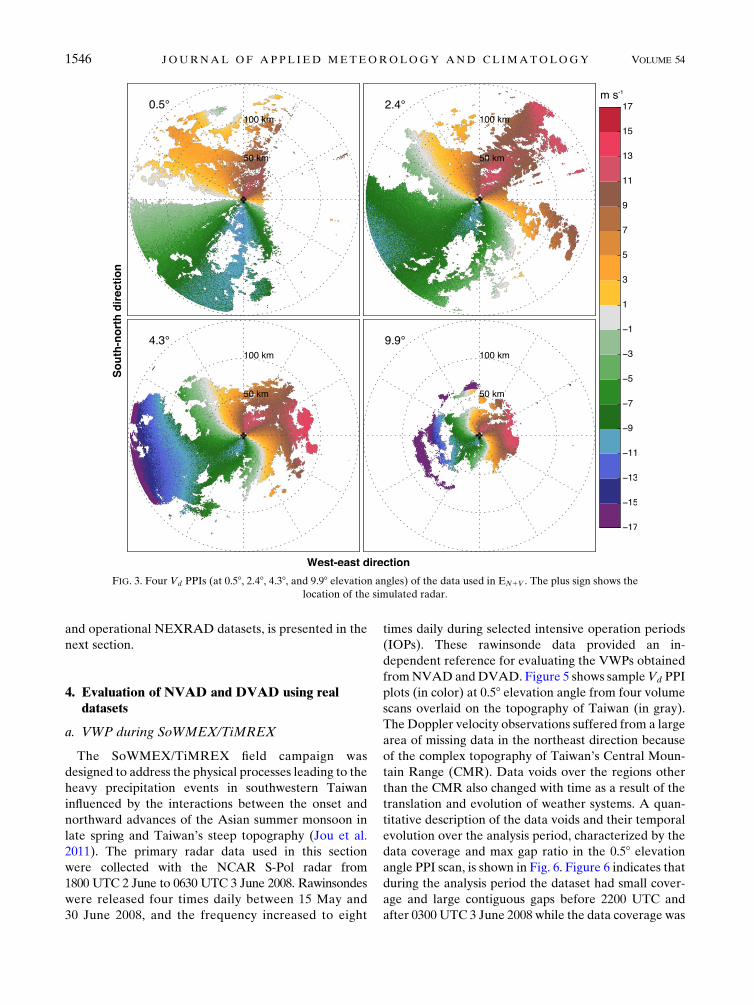
resultant volume data used in EN1V are shown in Fig. 3.
Figure 2c shows that the VWP derived from NVAD
deviates significantly from the true value, especially at
upper levels, while the VWP derived from DVAD is
generally not influenced by the same data noise and
voids. Possible reasons for the distinct results are dis-
cussed in the next subsection.
b. Limitations of NVAD method
The mathematical formulation of NVAD requires
two sequential LSFs to solve for the horizontal wind at
the radar site. The first step is similar to the traditional
VAD analysis with higher-order Fourier series used to
fit Vd on a VAD ring. The second step uses polynomial-
based functions to fit the Fourier coefficients obtained in
the first step at different ranges. After the nonlinearity is
taken into account explicitly, the two LSFs in NVAD
could both introduce uncertainties when Doppler ve-
locities contain noise and voids (e.g., EN1V).
The uncertainty in the first-step VAD analysis of
NVAD is closely related to data voids and noise in
observed Doppler velocities. As illustrated in Daley
(1993, 45–49), fitting observations of uneven density
(due to the existence of data voids) and noise is prone to
the overfitting problem, especially when higher-order
mathematical models are used. Data noise and voids are
inevitable in Doppler radar observations as a result of
weak signal, ground clutter, nonmeteorological objects,
abnormal propagation, beam blockage, and velocity
aliasing. Figure 4 and Table 1 present an example of an
incorrect VAD analysis caused by the overfitting prob-
lem in real observations. Figure 4a shows a PPI plot of
Doppler velocities observed at 0.58 elevation angle
during the SoWMEX/TiMREX field campaign. The
large black circle in Fig. 4a indicates the VAD ring used
to perform the VAD analysis. The fitted curves of dif-
ferent orders from this VAD ring are shown in Fig. 4b,
and the corresponding values of the first five Fourier
coefficients and their standard deviations (SDs) of fitting
are listed in Table 1. It is noted that the SD values of
fitting decrease monotonically with higher-order VAD
analyses, which indicates higher-order wind models fit
better to the observed data. The fitted curves in Fig. 4b
also demonstrate the same tendency where the curves of
FIG. 1. (a1)–(a3) Wind vectors and (b1)–(b3) Vd PPIs used in the OSE. The Vd PPIs are produced based upon the wind fields in
(a1)–(a3). The plus sign shows the location of the simulated radar. The circles in the same column [e.g., (a1) and (b1)] indicate the
locations where the conical surface of the PPI intercepts the corresponding constant-altitude plane of wind vectors.
1544 JOURNAL OF APPL IED METEOROLOGY AND CL IMATOLOGY VOLUME 54

higher-order models are closer to the observed data.
Nevertheless, a comparison of the two coefficients a1and b1 between the third- and fourth-order fitting re-
veals an abrupt change. Since the estimated wind field
from the single-Doppler velocity pattern in Fig. 4a is
approximately southwesterly, it is clear that the results
of the second- and third-order fitting are reasonable,
while the fourth-order fitting is clearly incorrect (the
wind direction is reversed) due to the overfitting
problem.
The uncertainty in the second-step polynomial anal-
ysis of NVAD can be understood by examining the SD
values listed in Table 1. Despite the incorrect results of
the fourth-order VAD analysis, its SD value of fitting is
nevertheless the smallest. NVAD uses the SD values of
the first step fitting as weights for the Fourier coefficients
used in the second step polynomial fitting. These phys-
ically incorrect coefficients will yield higher weights and
further contaminate the final results.
The two limitations of NVAD are mutually related
and essentially determined by the distribution of data
noise and voids. To better illustrate the impact of data
noise and voids on the accuracy of NVAD and DVAD
retrievals, an azimuthally continuous gap with in-
creasing width is added to EN. The results in Table 2
show that, as the width of the gap and the order of fitting
increase, the error of retrieval by NVAD increases ac-
cordingly while those of DVAD remain small. The
higher-order results of NVAD become unusable when
the gap width exceeds 1508. It is noted that when the
maximum gap width is greater than 1808 (not shown),the errors of both methods become significant and un-
usable. Table 3 shows that the DVAD result is not
sensitive to the azimuthal location of the gap. In real
weather observations, data noise and voids are not only
inevitable but also variable in both time and space. It is
difficult to examine the data quality of each VAD ring
of a volume scan used in NVAD and to rule out those
that could potentially lead to incorrect results.
Within the DVAD framework, linear and nonlinear
wind fields at a constant altitude are expressed as a
single polynomial function only with different orders.
Unlike CZ92, the VWP at the radar is directly resolved
with only a one-step 2D LSF whether the wind field is
linear or nonlinear. The greater redundancy of data used
in the 2D fitting process effectively reduces the over-
fitting problem and is able to overcome the limitations of
NVAD as demonstrated in EN1V. Although the above
experiments demonstrated the robust performance of
DVAD when processing simulated Doppler velocity
observations with noise and voids, they only provided a
specific scenario of the distribution of noise and voids,
while their distributions could vary greatly in real
weather systems. A more comprehensive comparison
between NVAD andDVAD as well as the limitations of
DVAD, using both SoWMEX/TiMREX field campaign
FIG. 2. A comparison of NVAD and DVAD using the ideal Doppler velocities. Here, ut and yt are the true horizontal winds while
unvad (udvad) and ynvad (ydvad) are the retrieved horizontal winds of NVAD (DVAD). (a) VWPs in an idealized wind field. (b) As in (a),
but with 2m s21 random noise. (c) As in (b), but with simulated data voids.
JULY 2015 TANG ET AL . 1545
and operational NEXRAD datasets, is presented in the
next section.
4. Evaluation of NVAD and DVAD using realdatasets
a. VWP during SoWMEX/TiMREX
The SoWMEX/TiMREX field campaign was
designed to address the physical processes leading to the
heavy precipitation events in southwestern Taiwan
influenced by the interactions between the onset and
northward advances of the Asian summer monsoon in
late spring and Taiwan’s steep topography (Jou et al.
2011). The primary radar data used in this section
were collected with the NCAR S-Pol radar from
1800 UTC 2 June to 0630 UTC 3 June 2008. Rawinsondes
were released four times daily between 15 May and
30 June 2008, and the frequency increased to eight
times daily during selected intensive operation periods
(IOPs). These rawinsonde data provided an in-
dependent reference for evaluating the VWPs obtained
fromNVAD andDVAD. Figure 5 shows sampleVd PPI
plots (in color) at 0.58 elevation angle from four volume
scans overlaid on the topography of Taiwan (in gray).
The Doppler velocity observations suffered from a large
area of missing data in the northeast direction because
of the complex topography of Taiwan’s Central Moun-
tain Range (CMR). Data voids over the regions other
than the CMR also changed with time as a result of the
translation and evolution of weather systems. A quan-
titative description of the data voids and their temporal
evolution over the analysis period, characterized by the
data coverage and max gap ratio in the 0.58 elevationangle PPI scan, is shown in Fig. 6. Figure 6 indicates that
during the analysis period the dataset had small cover-
age and large contiguous gaps before 2200 UTC and
after 0300 UTC 3 June 2008 while the data coverage was
FIG. 3. Four Vd PPIs (at 0.58, 2.48, 4.38, and 9.98 elevation angles) of the data used in EN1V . The plus sign shows the
location of the simulated radar.
1546 JOURNAL OF APPL IED METEOROLOGY AND CL IMATOLOGY VOLUME 54

relatively improved between those times. Only basic
data quality control procedures (ground-clutter removal
and Doppler velocity unfolding) were applied to this
dataset to create amore challenging set of conditions for
the tested methods. As will be shown in the following
analysis, the ground clutter and other artifacts have
important impacts on the retrieved winds at lower
altitudes.
Figure 7 shows retrieved VWPs using second-order
nonlinear wind models to approximate the real wind
field. For the purpose of verification, the sounding data
from the Pingtung rawinsonde site in southern Taiwan
(blue plus sign in Fig. 5) are included for comparison
with results from NVAD and DVAD. It is noteworthy
that the rawinsonde measures a wind profile along the
trajectory of the balloon, while the VWPs obtained from
Doppler radar (both NVAD and DVAD) represent
compatible winds over the large area covered by the
radar. Close agreement between the two types of VWPs
is not expected (CZ92). Nevertheless, good agreement
between the radar-derived VWP with that of the ra-
winsonde confirms the representativeness of the VWP
obtained from NVAD and/or DVAD.
During the analysis time period, a cold front
approached the S-Pol domain from the northwest and
passed the S-Pol site at’0100 UTC 3 June 2008. The
southwest-to-northwest veering of wind vectors over
time associated with the passage of this cold front was
clearly delineated in both VWPs from NVAD and
DVAD. Both VWPs showed greater variations of wind
direction and speed over time at lower altitudes than at
higher altitudes, consistent with the passage of a trough
at low to midlevels. There were four soundings released
from the Pingtung rawinsonde site during the same time
period. When compared with the sounding profile (red
wind barbs), both VWPs from NVAD and DVAD
compared favorably to those from the Pingtung rawin-
sonde site. It is noted that the VWPs deduced by both
FIG. 4. An example of imperfect data contaminating the results
of a higher-order VAD analysis. (a) A PPI plot at 0.58 elevationangle in a volume scan from the SoWMEX/TiMREX field cam-
paign. The black circle shows the data points used for the VAD
analysis. (b) Scatterplots of data on the circle in (a) and fitted
values of different-order Fourier analyses.
TABLE 1. The first five Fourier coefficients and SD of fitting from
high-order VAD analyses. Under the linear assumption, a0, a1, b1,
a2, and b2 are related to the mean values of divergence, horizontal
wind (u0, y0), stretching, and shearing deformation of the wind field.
Order a0 a1 b1 a2 b2 SD
2 23.42 6.39 7.38 22.27 23.99 1.6
3 0.96 14.67 7.93 4.01 22.12 1.4
4 214.70 27.86 0.47 212.31 24.55 1.1
TABLE 2. Speed errors (m s21) of DVAD and NVAD subjected to different continuous gap sizes (308, 608, 908, 1208, and 1508).
308 608 908 1208 1508
Order DVAD NVAD DVAD NVAD DVAD NVAD DVAD NVAD DVAD NVAD
2 1.6 2.4 1.8 2.7 1.8 2.9 1.4 3.2 1.5 3.0
3 1.6 2.7 1.7 2.9 1.7 2.8 1.8 2.0 2.8 3.6
4 1.7 1.7 1.7 1.7 1.7 2.4 1.6 3.2 1.6 20.7
5 1.7 2.4 1.7 2.4 1.7 2.5 1.6 13.2 1.2 57.0
JULY 2015 TANG ET AL . 1547

methods consistently have the greatest error at lower
altitudes. This error is related to the increased non-
linearity of the wind field and the decreased data quality
at lower levels.
Figure 8 shows retrieved VWPs using fourth-order
nonlinear wind models to approximate the real wind
field. When the fourth-order nonlinear model was used,
there were significant differences between the results of
the two methods. As shown in Fig. 8a, the result of the
NVAD method had abnormal and extreme values at
different altitudes and times (e.g., 2000, 2230, and
0200 UTC). The missing wind barbs between 2000 and
2100 UTC were outliers where wind speed was greater
than 40ms21. It is noted that the occurrences of incon-
sistent and unreasonable results were intermittent, which
was probably caused by the temporal variation of data
voids. The result of DVAD using a fourth-order non-
linear model was consistent with that of the second-
order model and compared favorably to the sounding
data. The southwest-to-northwest veering of wind direc-
tion over time was still clearly shown by the time series of
VWPs in Fig. 8b. Even-higher-order nonlinear models
were used to retrieve VWPs at the S-Pol site, and the
TABLE 3. Speed errors (m s21) of DVAD subjected to a 1808azimuthally continuous gap placed in different directions.
Order East South West North
2 2.6 2.3 2.7 3.1
3 1.5 2.3 2.5 4.0
4 2.0 2.4 1.0 2.4
5 3.4 2.9 2.6 2.8
FIG. 5. SampleVd PPI plots at 0.58 elevation of four volume scans collected at 2000 and 2300UTC 2 Jun 2008 and at
0100 and 0400 UTC 3 Jun 2008 overlaid on the topography of Taiwan. The blue plus sign shows the location of the
Pingtung rawinsonde site.
1548 JOURNAL OF APPL IED METEOROLOGY AND CL IMATOLOGY VOLUME 54

results (not shown) were similar to those in Fig. 8,
where NVAD showed more incorrect results while
DVAD continued to show consistent results with the
sounding data.
In the calculation of Figs. 7 and 8, all Doppler velocity
observations within the maximum range (150 km) of the
S-Pol radar were used. It is possible to select only
Doppler observations within a certain distance from the
radar. Figure 9 shows VWPs retrieved in the same
way as those in Fig. 8, but using Doppler velocity
observations within 100 km from the radar. It is clear
that the retrieved VWPs are consistent with those in
Fig. 8, which indicates that neither method is sensitive to
the range of data used for calculation. Figures 7–9
demonstrate the improvement of DVAD over NVAD
when higher-order models are used; the performance of
the different orders of DVAD will be addressed in
section 5.
b. VWP using NEXRAD datasets
The results using the dataset from the SoWMEX/
TiMREX field campaign demonstrate that DVAD is
generally more robust than NVAD when dealing with
real observations contaminated by noise and data voids.
FIG. 6. Data coverage and maximum contiguous gap ratio at 0.58elevation angle from 1800 UTC 2 Jun to 0630 UTC 3 Jun 2008. The
data coverage ratio is defined by the number of bins with valid
Doppler velocity divided by the total number of bins in a PPI scan.
The ‘‘max gap’’ ratio is defined by the average of the maximum
contiguous gap along the azimuthal direction of each gate divided
by the total number of rays.
FIG. 7. Time series of VWPs computed by (a) NVAD and
(b) DVAD using a second-order nonlinear wind model. VWPs
from the Pingtung rawinsonde site at four different times are shown
as red wind barbs. Wind barbs are plotted every 1 km from 0.5 km
above radar level and every 40min in time. The vertical dashed line
indicates the approximate time at which the cold front passed the
radar site.
FIG. 8. As in Fig. 7, but using a fourth-order nonlinear wind model.
FIG. 9. As in Fig. 8, but using data within a 100-km radius.
JULY 2015 TANG ET AL . 1549
In this section, two winter storm cases collected by the
operational NEXRADs were used to examine the per-
formance of NVAD and DVAD under different
weather regimes and geographic locations.
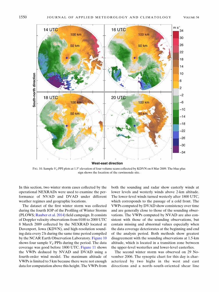
The dataset of the first winter storm was collected
during the fourth IOP of the Profiling of Winter Storms
(PLOWS; Rauber et al. 2014) field campaign. It consists
of Doppler velocity observations from 0100 to 2000 UTC
8 March 2009 collected by the NEXRAD located at
Davenport, Iowa (KDVN), and high-resolution sound-
ing data every 2 h during the same time period compiled
by the NCAR Earth Observation Laboratory. Figure 10
shows four sample Vd PPIs during the period. The data
coverage was good before 1800 UTC. Figure 11 shows
the VWPs deduced by NVAD and DVAD using a
fourth-order wind model. The maximum altitude of
VWPs is limited to 5 km because there were not enough
data for computation above this height. The VWPs from
both the sounding and radar show easterly winds at
lower levels and westerly winds above 2-km altitude.
The lower-level winds turned westerly after 1800 UTC,
which corresponds to the passage of a cold front. The
VWPs computed by DVAD show consistency over time
and are generally close to those of the sounding obser-
vations. The VWPs computed by NVAD are also con-
sistent with those of the sounding observations, but
contain missing and abnormal values especially when
the data coverage deteriorates at the beginning and end
of the analysis period. Both methods show greatest
disagreement with the sounding observations at 1.5-km
altitude, which is located in a transition zone between
the upper-level westerlies and lower-level easterlies.
The second winter storm was observed on 29 No-
vember 2006. The synoptic chart for this day is char-
acterized by two highs in the west and east
directions and a north–south-oriented shear line
FIG. 10. SampleVd PPI plots at 1.58 elevation of four volume scans collected by KDVN on 8Mar 2009. The blue plus
sign shows the location of the rawinsonde site.
1550 JOURNAL OF APPL IED METEOROLOGY AND CL IMATOLOGY VOLUME 54

(http://www.hpc.ncep.noaa.gov/dailywxmap/). The
NEXRAD dataset during 0800–2000 UTC 29 November
2006 from KDVN is used because there is a Global
Telecommunication System (GTS) sounding site near the
radar for verification. The sounding site records obser-
vations 2 times per day at 0000 and 1200 UTC. Thus,
there is only one sounding VWP for verification during
the period of radar observation. Figure 12 shows four
sampleVd PPIs at different times. Before 1500UTC (and
after 1700UTC, which is not shown), there are large data
voids in the radar domain as a result of the precipitation
structure of the storm. Figure 13 shows the computed
VWPs from both NVAD and DVAD. The VWPs from
DVAD show consistent southwesterly winds above 1-km
altitude that correspond well to the upper-level trough in
the synoptic chart. Horizontal winds veer over time and
correspond well to the passage of a cold front over the
radar site at around 1230 UTC. The winds at 1200 UTC
are consistent with those observed by the nearby sound-
ing site. The upper-level southwesterly and veering
lower-level winds are also revealed by NVAD, but the
results are contaminated bymissing and abnormal values.
5. Objective estimation of nonlinearity
When extending the single-Doppler analysis from lin-
ear to nonlinear windmodels, one of the critical questions
is how many nonlinear terms of a wind model are
necessary to sufficiently represent the real wind field.
CZ92 did not specify how to determine the optimal order
of NVAD to represent the wind field, and the degree of
nonlinearity was empirically estimated before the com-
putation. Previous studies (Waldteufel and Cobin 1979;
Koscielny et al. 1982; Boccippio 1995) have shown that
the results of single-Doppler analyses canbe biased by the
underfitting or overfitting problem due to the choice of an
improper wind model. One must be able to dynamically
and objectively adjust the nonlinear wind model for best
results, especially for operational purposes.
The mathematical models for different orders of non-
linear wind fields used in NVAD and DVAD are nested,
which means that the coefficients of a lower-order model
are strictly a subset of those of a higher-order model. The
standard way of determining the optimal model out of
such nested models is to perform an F test (Wilks 2011).
An F test basically compares the residual sum of squares
(RSS) between higher- and lower-order models to de-
termine if the higher-order model is still necessary. Since
two LSFs are used in the NVAD method, and each LSF
has its own RSS value, it is not straightforward to de-
termine the goodness of fit of the two steps combined.
Furthermore, incorrect Fourier fitting may still have
small RSS values (RSS is proportional to SD) because of
the overfitting problem shown in previous sections; the
small RSS values in NVAD may not truly indicate
the goodness of fit. In the DVADmethod, the RSS of the
entire domain at each analysis altitude can be directly
obtained since only a one-step fitting is required, and the
RSS is more representative of the goodness of fit of the
mathematical model to the true wind field. Moreover,
since the calculation of DVAD uses Doppler velocity
observations within a finite vertical extent, the differ-
ences in nonlinearity at different altitudes can be esti-
mated independently. The independent evaluation of
nonlinearity at different altitudes is not possible in
NVAD because the vertical variation of the wind field is
forced to be the same as those of the horizontal winds a
priori. It has been shown that real wind fields have dif-
ferent degrees of nonlinearity at different altitudes
(CZ92); therefore, the DVAD method is likely to pro-
ducemore accurate VWPs throughout the vertical extent
of the analysis domain.
An F test requires that the data samples used in the
fitting model are independent. Since spatially adjacent
radar observations are essentially dependent, the stan-
dard F test is not applicable here. Following the princi-
ple of the F test, the coefficient of determination R2,
defined as
R25 12RSS
TSS, (15)
FIG. 11. Time series of VWPs computed by (a) NVAD and
(b) DVAD using Doppler velocity observations collected by
KDVN on 8 Mar 2009. VWPs from a nearby rawinsonde site (the
blue plus sign in Fig. 10) are shown as red wind barbs. Wind barbs
are plotted every 0.5 km from 0.5 km above radar level and every
hour in time. The vertical dashed line indicates the approximate
time when the cold front passed the radar site.
JULY 2015 TANG ET AL . 1551

is used to determine a proper nonlinear model for real
wind fields. Here, TSS is the total sum of squares of the
observation data. The value of R2 measures the ratio of
the explained variance by the nonlinear wind model to
the total variance of observations, which is consistent
with the idea of the F test. By comparing the values ofR2
for two consecutive orders of a fitting model, defined as
Im 5R2high
R2low
2 1, (16)
the relative improvement of using a higher-order model
can be estimated. The practical procedure of de-
termining the optimal order is as follows: the R2 value
of a linear wind model is first calculated as a reference
value, and then R2 values of higher-order models are
calculated sequentially. After calculating the R2 value
of a higher-order nonlinear wind model each time, the
value of Im is calculated according to (16). The same
procedure is repeated until Im reaches a predefined
threshold, which indicates that no more variance in the
data can be explained by the higher-order model.
Table 4 shows an example of Im calculated with re-
spect to different orders (up to seven) and altitudes us-
ing the same OSE data (EN1V) shown in the previous
section. The large values of Im of the lower-order
models, especially at the lower levels, indicate that
higher-order models are necessary. In other words,
higher-order models of DVAD generally give more
accurate results. Note that the Im values stayed small
after reaching a small value, whichmeans that increasing
the order of DVAD will not bring any significant im-
provement beyond a certain order. This characteristic
can be used as a criterion for determining the optimal
order for a nonlinear wind field. After experimenting
with a large set of SoWMEX/TiMREX data, it was
FIG. 12. SampleVd PPI plots at 1.58 elevation of four volume scans collected byKDVNon 29Nov 2009. The blue plus
sign shows the location of the GTS rawinsonde site.
1552 JOURNAL OF APPL IED METEOROLOGY AND CL IMATOLOGY VOLUME 54

found that the value of 0.5% was a reasonable threshold
for determining the optimal order. Table 4 shows a
higher degree of the nonlinear wind field at low levels, as
well as a quasi-linear wind field above 5km. This result
was consistent with the characteristics of wind fields
shown in Fig. 1.
The objective procedure was applied to the same
Doppler velocity observations from the SoMWEX/
TiMREX field campaign. The retrieved VWPs along-
side the objectively determined orders of nonlinear
winds are shown in Fig. 14. The retrieved VWPs in
Fig. 14a were consistent with Fig. 8b using fourth-order
uniformly and compared favorably to the sounding
VWPs. The determined orders of the nonlinear wind
model shown in Fig. 14b provide some insights into the
structure and variation of the wind field being examined.
Figure 14b first shows that a higher-order wind model is
generally required at lower levels. This is consistent with
the increased variabilities of the wind field near the
ground. Before 0100 UTC 3 June 2008 when the cold
front moved into the radar scope, the nonlinearity of the
wind field at lower levels was generally lower. During
the passage of the cold front, the wind field with the
radar scope consisted of both northwesterly and south-
westerly winds, and Fig. 14b shows an increased order of
the nonlinear wind field accordingly.
6. Summary and conclusions
In this study, the DVAD method was used to quan-
titatively analyze nonlinear wind fields observed by a
single-Doppler radar. DVAD uses rVd as the variable
for analyzing Doppler velocity observations at a con-
stant altitude. The rVd field of linear and nonlinear wind
fields observed by a single-Doppler radar at each alti-
tude was expressed in a single and concise 2D poly-
nomial function. Only a one-step LSF of a 2D
polynomial function to the observed Doppler velocities
was required to obtain the physical parameters of a real
wind field. The new method was compared with the
traditional nonlinear wind analysis method, namely
NVAD, which uses two separate LSFs to solve for the
same information. It was demonstrated that the VWPs
retrieved by both DVAD and NVADwere consistent in
ideal conditions. Both methods were robust to the ex-
istence of random noise without data voids. Neverthe-
less, when noisy data were unevenly distributed because
of data voids, the difference between theVWPs deduced
by the two methods became significant. The NVAD-
derived VWP showed large deviations from the rawin-
sondeVWP,whileDVADshowed consistent and robust
results. The different VWPs were attributed to the
overfitting problem when higher-order VAD analyses
were used with unevenly distributed noisy data. The
FIG. 13. As in Fig. 11, but using data from a winter storm col-
lected by KDVNon 29 Nov 2006. The wind barbs are plotted every
40min in time.
TABLE 4. The Im values (3100) of different orders of DVAD
analyses at different altitudes.
Height (km) Second Third Fourth Fifth Sixth Seventh
1 9.2 4.6 1.6 1.4 0.5 0.3
3 1.5 2.4 0.1 0.3 0.1 0.1
5 0.6 0.7 0.0 0.1 0.0 0.0
7 0.4 0.2 0.0 0.0 0.0 0.0
FIG. 14. Time series of (a) VWPs computed by DVAD in which
the order of the nonlinear wind model is determined objectively,
and (b) the magnitudes of those orders. VWPs from the Pingtung
rawinsonde site at four different times are shown as red wind barbs.
JULY 2015 TANG ET AL . 1553

robust performance of DVAD was further demon-
strated with real Doppler velocity observations from the
SoWMEX/TiMREXfield campaign and the operational
NEXRAD network.
The use of only a one-step LSF in DVAD allows for
the direct estimation of the degree of nonlinearity in real
wind fields. The same estimation is not feasible in
NVADbecause two separate LSFs are used. An optimal
nonlinear windmodel to approximate the real wind field
can be objectively determined during the analysis by
comparing the R2 values of different wind models. The
degree of nonlinearity at different altitudes can also be
assessed because the analyses at different altitudes are
independent in DVAD. This feature is instrumental in
understanding the vertical structure of the wind field and
is important in alleviating both overfitting and under-
fitting. The degree of nonlinearity at different altitudes
determined by DVAD was shown to be consistent with
the characteristics of the original wind field.
The study shows the potential of DVAD as a quan-
titative analysis tool for single-Doppler radar observa-
tions beyond the qualitative interpretation presented in
Lee et al. (2014). Although the case studies presented in
this study demonstrate that DVAD is generally more
robust than NVAD, they by no means suggest that the
performance of DVAD is universally robust. In addition
to the operational limitations mentioned in previous
sections, DVAD is subject to the same fundamental
limitation as that of VAD and NVAD. All of these
single-Doppler analysis methods are based on a pre-
scribed wind model, which results from a truncated
Taylor expansion. The methods are essentially limited
by the extent to which real wind fields can be repre-
sented by such a truncated Taylor expansion. In addi-
tion, as discussed in Lee et al. (2014), although DVAD
simplifies the interpretation of single-Doppler observa-
tions, the vorticity still cannot be retrieved regardless
of either the linear or nonlinear wind fields. Therefore,
the method proposed in this study cannot be used in
flow fields where the vorticity dominates (e.g., mature
tropical cyclones). Despite its own limitations, the sim-
plicity and robust performance of the DVAD method
make it a good candidate for single-Doppler analysis in
operational use.
Acknowledgments. The authors thank Dr. Scott Ellis
andDr.Wei-YuChang for their helpful comments on the
manuscript and Dr. Juanzhen Sun for providing the
model output of the squall-line simulation. Comments
and suggestions by three anonymous reviewers greatly
improved the manuscript. The first author is grateful for
the support by the Graduate Student Visitor Program of
the NCAR Advanced Study Program (ASP) and the
Earth Observing Laboratory (EOL) during this research.
This study is supported by National Fundamental Re-
search 973 Program of China (2015CB452801) and the
research fund of the Key Laboratory of Transportation
Meteorology (BJG201202).
REFERENCES
Armijo, L., 1969: A theory for the determination of wind and
precipitation velocities with Doppler radars. J. Atmos.
Sci., 26, 570–573, doi:10.1175/1520-0469(1969)026,0570:
ATFTDO.2.0.CO;2.
Bluestein, H. B., and D. S. Hazen, 1989: Doppler-radar analysis
of a tropical cyclone over land: Hurricane Alicia (1983) in
Oklahoma. Mon. Wea. Rev., 117, 2594–2611, doi:10.1175/
1520-0493(1989)117,2594:DRAOAT.2.0.CO;2.
——, C. C. Weiss, and A. L. Pazmany, 2004: Doppler radar obser-
vations of dust devils in Texas. Mon. Wea. Rev., 132, 209–224,
doi:10.1175/1520-0493(2004)132,0209:DROODD.2.0.CO;2.
Boccippio, D. J., 1995: A diagnostic analysis of the VVP single-
Doppler retrieval technique. J. Atmos.Oceanic Technol., 12, 230–
248, doi:10.1175/1520-0426(1995)012,0230:ADAOTV.2.0.CO;2.
Browning, K. A., and R. Wexler, 1968: The determination of kine-
matic properties of a wind field using Doppler radar. J. Appl.
Meteor., 7, 105–113, doi:10.1175/1520-0450(1968)007,0105:
TDOKPO.2.0.CO;2.
Caya, D., and I. Zawadzki, 1992: VAD analysis of nonlinear wind
fields. J. Atmos. Oceanic Technol., 9, 575–587, doi:10.1175/
1520-0426(1992)009,0575:VAONWF.2.0.CO;2.
Chrisman, J., and S. Smith, 2009: Enhanced velocity azimuth dis-
play wind profile (EVWP) function for the WSR-88D. Pre-
prints, 34th Conf. on RadarMeteor.,Williamsburg, VA,Amer.
Meteor. Soc., P4.7. [Available online at https://ams.confex.com/
ams/pdfpapers/155822.pdf.]
Daley, R., 1993:AtmosphericDataAnalysis.CambridgeUniversity
Press, 472 pp.
Davis, C. A., and W.-C. Lee, 2012: Mesoscale analysis of heavy
rainfall episodes from SoWMEX/TiMREX. J. Atmos. Sci., 69,
521–537, doi:10.1175/JAS-D-11-0120.1.
Doviak, R. J., and D. S. Zrnic, 2006: Doppler Radar and Weather
Observations. 2nd ed. Dover, 592 pp.
Giammanco, I. M., J. L. Schroeder, and M. D. Powell, 2013: GPS
dropwindsonde and WSR-88D observations of tropical cy-
clone vertical wind profiles and their characteristics. Wea.
Forecasting, 28, 77–99, doi:10.1175/WAF-D-11-00155.1.
Houze, R. A., Jr., 2004: Mesoscale convective systems. Rev. Geo-
phys., 42, 1–43, doi:10.1029/2004RG000150.
Jou, B., W. Lee, and R. Johnson, 2011: An overview of SoWMEX/
TiMREX and its operation. The Global Monsoon System:
Research and Forecast, C.-P. Chang, Ed., 2nd ed., World Sci-
entific, 303–318.
Kingsmill, D. E., P. J. Neiman, B. J.Moore,M.Hughes, S. E. Yuter,
and F. M. Ralph, 2013: Kinematic and thermodynamic struc-
tures of Sierra barrier jets and overrunning atmospheric rivers
during a landfalling winter storm in northern California.Mon.
Wea. Rev., 141, 2015–2036, doi:10.1175/MWR-D-12-00277.1.
Kollias, P., B. A. Albrecht, R. Lhermitte, andA. Savtchenko, 2001:
Radar observations of updrafts, downdrafts, and turbulence in
fair-weather cumuli. J. Atmos. Sci., 58, 1750–1766, doi:10.1175/
1520-0469(2001)058,1750:ROOUDA.2.0.CO;2.
Koscielny, A. J., R. J. Doviak, and R. Rabin, 1982: Statistical consid-
erations in the estimation of divergence from single-Doppler
1554 JOURNAL OF APPL IED METEOROLOGY AND CL IMATOLOGY VOLUME 54
radar and application to prestorm boundary-layer observations.
J.Appl.Meteor.,21,197–210,doi:10.1175/1520-0450(1982)021,0197:
SCITEO.2.0.CO;2.
Lee, W.-C., F. D. Marks, and R. E. Carbone, 1994: Velocity track
display—A technique to extract real-time tropical cyclone circu-
lations using a single airborne Doppler radar. J. Atmos. Oceanic
Technol., 11, 337–356, doi:10.1175/1520-0426(1994)011,0337:
VTDTTE.2.0.CO;2.
——, B. J.-D. Jou, P.-L. Chang, and S.-M. Deng, 1999: Tropical
cyclone kinematic structure retrieved from single-Doppler
radar observations. Part I: Interpretation of Doppler ve-
locity patterns and the GBVTD technique.Mon.Wea. Rev.,
127, 2419–2439, doi:10.1175/1520-0493(1999)127,2419:
TCKSRF.2.0.CO;2.
——, X. Tang, and B. J.-D. Jou, 2014: Distance velocity azimuth
display (DVAD) new interpretation and analysis of Doppler
velocity. Mon. Wea. Rev., 142, 573–589, doi:10.1175/
MWR-D-13-00196.1.
Lhermitte, R.M., andD.Atlas, 1961: Precipitationmotion by pulse
Doppler. Proc. Ninth Weather Radar Conference, Boston,
MA, Amer. Meteor. Soc., 218–223.
Matejka, T. J., and R. C. Srivastava, 1991: An improved version of
the extended velocity-azimuth display analysis of single-
Doppler radar data. J. Atmos. Oceanic Technol., 8, 453–466,
doi:10.1175/1520-0426(1991)008,0453:AIVOTE.2.0.CO;2.
Peace, R. L., Jr., R. A. Brown, and H. Camnitz, 1969: Horizontal
motion field observationswith a singleDoppler radar. J. Atmos.
Sci., 26, 1096–1103, doi:10.1175/1520-0469(1969)026,1096:
HMFOWA.2.0.CO;2.
Rabin, R., and I. Zawadzki, 1984: On the single-Doppler measure-
ments of divergence in clear air. J.Atmos.OceanicTechnol., 1, 50–
75, doi:10.1175/1520-0426(1984)001,0050:OTSDMO.2.0.CO;2.
Rauber, R. M., and Coauthors, 2014: Stability and charging char-
acteristics of the comma head region of continental winter
cyclones. J. Atmos. Sci., 71, 1559–1582, doi:10.1175/
JAS-D-13-0253.1.
Rinehart, R., and E. T. Garvey, 1978: Three-dimensional storm
motion detection by conventional weather radar. Nature, 273,
287–289, doi:10.1038/273287a0.
Srivastava, R. C., and T. J. Matejka, 1986: Doppler radar study of
the trailing anvil region associated with a squall line. J. Atmos.
Sci., 43, 356–377, doi:10.1175/1520-0469(1986)043,0356:
DRSOTT.2.0.CO;2.
Sun, J., and Y. Zhang, 2008: Analysis and prediction of a squall line
observed during IHOP using multiple WSR-88D observations.
Mon.Wea. Rev., 136, 2364–2388, doi:10.1175/2007MWR2205.1.
Tuttle, J. D., andG. B. Foote, 1990: Determination of the boundary
layer airflow from a single Doppler radar. J. Atmos. Oceanic
Technol., 7, 218–232, doi:10.1175/1520-0426(1990)007,0218:
DOTBLA.2.0.CO;2.
——, and R. Gall, 1999: A single-radar technique for estimating the
winds in tropical cyclones.Bull. Amer.Meteor. Soc., 80, 653–668,doi:10.1175/1520-0477(1999)080,0653:ASRTFE.2.0.CO;2.
Waldteufel, P., and H. Cobin, 1979: On the analysis of single-
Doppler radar data. J. Appl. Meteor., 18, 532–542, doi:10.1175/1520-0450(1979)018,0532:OTAOSD.2.0.CO;2.
Wilks, D. S., 2011: Statistical Methods in the Atmospheric Sciences.
3rd ed. Academic Press, 676 pp.
JULY 2015 TANG ET AL . 1555