nonmonotone derivate–free methods for nonlinear equations
TRANSCRIPT

Nonmonotone derivate–free methodsfor nonlinear equations
Luigi Grippo and Marco Sciandrone
Technical Report n. 12005
Dipartimento di Informatica e Sistemistica “Antonio Ruberti”Università degli Studi di Roma “La Sapienza”
ARACNE

I Technical Reports del Dipartimento di Informatica e Sistemistica “Antonio Ruberti”svolgono la funzione di divulgare tempestivamente, in forma definitiva o provvisoria, i risultati diricerche scientifiche originali. Per ciascuna pubblicazione vengono soddisfatti gli obblighi previstidall’art. 1 del D.L.L. 31.8.1945, n. 660 e successive modifiche.Copie della presente pubblicazione possono essere richieste alla Redazione.
Dipartimento di Informatica e Sistemistica “Antonio Ruberti”Università degli Studi di Roma “La Sapienza”
Via Eudossiana, 18 - 00184 RomaVia Buonarroti, 12 - 00185 RomaVia Salaria, 113 - 00198 Roma
www.dis.uniroma1.it
Copyright © MMVARACNE EDITRICE S.r.l.
Redazione :00173 Romavia Raffaele Garofalo, 133 A/B(06) 72672222 – (06) 93781065telefax 72672233
ISBN 88–548–0024-4
I diritti di traduzione, di memorizzazione elettronica,di riproduzione e di adattamento anche parziale,con qualsiasi mezzo, sono riservati per tutti i Paesi.
I edizione: marzo 2005
Finito di stampare nel mese di marzo del 2004dalla tipografia « Grafica Editrice Romana S.r.l. » di Romaper conto della « Aracne editrice S.r.l. » di RomaPrinted in Italy

Nonmonotone derivative-free methodsfor nonlinear equations1
L. Grippo∗ and M. Sciandrone∗∗
∗Universita di Roma “La Sapienza”Dipartimento di Informatica e SistemisticaVia Buonarroti 12 - 00185 Roma - Italy
∗∗Istituto di Analisi dei Sistemi ed Informatica del CNRViale Manzoni 30 - 00185 Roma - Italy
e-mail (Grippo): [email protected] (Sciandrone): [email protected]
Technical Report 01-05, DIS January 2005
ABSTRACT
In this paper we study nonmonotone globalization techniques, in con-nection with iterative derivative-free methods for solving a system ofnonlinear equations in several variables. First we define and analyzea class of nonmonotone derivative-free linesearch techniques for uncon-strained minimization of differentiable functions. Then we introduce aglobalization scheme, which combines nonmonotone watchdog rules andnonmonotone linesearches, and we study the application of this schemeto some recent extensions of the Barzilai-Borwein gradient method andto hybrid stabilization algorithms employing linesearches along coordi-nate directions. Numerical results on a set of standard test problemsshow that the proposed techniques can be of value in the solution oflarge dimensional systems of equations.
Keywords Nonmonotone techniques, derivative-free linesearch, Barzilai-Borwein method, nonlinear equations; hybrid methods.
1This work was supported in part by Project CNR/MIUR “Metodi e sistemi disupporto alle decisioni” and in part by MIUR, FIRB 2001 Research Program LargeScale Nonlinear Optimization, Roma, Italy.

1 Introduction
We consider the problem of solving a system of n nonlinear equations
F (x) = 0
in n real variables, by means of iterative methods. When n is large andthe Jacobian matrix is not available, because, for instance, of storage orcomputing time limitations, three basic approaches can be undertaken.The first can be that of employing fixed point iterations, which requireonly the knowledge of F and use the (possibly scaled) vector of residualsas search direction in the space of variables. A second approach can bethat of using some finite-difference/inexact Newton-type method, basedon Krylov subspace projections, which require the approximation of theaction of the Jacobian matrix times a vector and maintain the fast localconvergence properties of Newton’s method (see, e.g. [1]). The last,less studied, possibility can be that of employing some limited memoryversion of Broyden’s method (see, e.g. [23]).In the computational implementation of these methods, a major issue isthe definition of a globalization technique for ensuring convergence frompoor initial approximations of the solution. The typical approach isthat of introducing a merit function, such as, for instance, the functionf(x) = (1/2)‖F (x)‖2, and then using some linesearch or trust regionstrategy for the minimization of f (see, e.g. [5], [16]). Under suitableassumptions, convergence towards solutions of the nonlinear system canbe guaranteed, in principle, using appropriate minimization algorithms.However, as the derivatives of F are not available, the globalizationalgorithm should not require the knowledge of the gradient of the meritfunction f and hence, in order to establish convergence results, we mustemploy finite-difference approximations or rely on the available theoryon global convergence and stabilization of derivative-free methods (see,e.g. [12], [17]).
In the present paper we restrict our attention to derivative-free glob-alization techniques for fixed point methods, based on the iteration
xk+1 = xk − (1/αk
)F (xk), (1)
where αk ∈ R is a scaling parameter and x0 ∈ Rn is a given initial point.More specifically, we refer to a recent interesting proposal [18], where thescaling parameter αk (which can be positive or negative) is computedusing an extension to nonlinear equations of the Barzilai-Borwein (BB)stepsize [2], [9].
2

The globalization strategy proposed in [18] is based on computing astepsize λk ∈ (0, 1] along dk = −F (xk)/αk through the nonmonotonelinesearch introduced in [12], employing the acceptance condition
f(xk + λkdk) ≤ max0≤j≤min(k,M)
[f(xk−j)] + γλk∇f(xk)T dk, (2)
where γ ∈ (0, 1), M ≥ 0 is a given integer and ∇f(xk)T dk is approx-imated by means of a forward difference formula. The sign of the ap-proximated value of ∇f(xk)T dk is also used for defining the sign of thesearch direction. Convergence conditions for the method that incor-porates these rules require, in principle, that the gradient of f is notorthogonal to F . In spite of this, the computational results reported in[18] show that the method, called the SANE algorithm, is competitive,in terms of computing times, in comparison with various Newton-typemethods. More recently, a different linesearch technique has been de-fined in [19] and it is based on a modified version of the derivative-freelinesearch introduced in [20] for globalizing Broyden-like methods. Morespecifically, the acceptance rule can be written as
f(xk + λkdk) ≤ max0≤j≤min(k,M)
[f(xk−j)] + ηk − γλ2‖dk‖2,
where it is assumed that
0 <∑
k
ηk ≤ η < ∞.
The adoption of this rule avoids at all the need of approximating the di-rectional derivative ∇f(xk)T dk by finite differences, but convergence canbe still guaranteed, under essentially the same assumptions employed in[18], by excluding that ∇f(x)T F (x) = 0 at limit points that are not so-lutions of the nonlinear equations. The computational results reportedin [19] show that the new algorithm, called DF-SANE algorithm, is com-petitive and often more efficient than the SANE algorithm.
In this paper, we introduce new nonmonotone globalization schemes,based on a combination of nonmonotone derivative-free linesearches withnonmonotone watchdog rules [3]. The main motivation is that the accep-tance condition (2) enforces all the points generated by the algorithm toremain in the level set corresponding to the starting point x0, so that,in difficult cases, the behavior of the method may depend critically onthe choice of the starting point and on the value of M . The adoptionof watchdog criteria permits a further relaxation of the monotonicityrequirements, by admitting that the objective function may take any(reasonable) value during a limited number of iterations.
3

Nonmonotone strategies with similar objectives has been introduced in[11] in the context of Newton-type methods for unconstrained mini-mization and have been employed also for globalizing Gauss-Newtonmethods for nonlinear equations [8] and algorithms for nonlinear com-plementary problems [6]. More recently, a nonmonotone strategy basedon this idea [15] has been successfully employed in connection with theBarzilai-Borwein gradient method for unconstrained minimization [25].This strategy ensures that the unmodified BB scaling parameter αk canbe used during a finite set of iterations and also permits the adoption,in sequence, of different formulas for computation of αk. The tenta-tive points are accepted, provided that a nonmonotone acceptance rulesbased on the objective function values is satisfied. During this phase,no requirement is imposed on the search directions, which are not evenrequired to be descent directions. In case of failure after a prefixed num-ber of iterations, we backtrack to the last accepted point and perform alinesearch using a nonmonotone derivative-free technique along a searchdirection related to the residual. In particular, the linesearch schemesconsidered here are based on the derivative-free linesearches introducedfor unconstrained optimization (see, for instance [4], [12], [21]) and admitboth the possibility of starting from a variable initial stepsize and theexpansion of the initial tentative step through an extrapolation phase.
It is shown, by extending some of the results of [15], that a global-ization algorithm based on these criteria retains the same convergenceproperties of the techniques proposed in [18] and [19], so that convergencecan be guaranteed, under usual continuity and compactness assumptions,provided that ∇f(x)T F (x) 6= 0 at points that are not solutions of thesystem.
In order to overcome this limitation, we define also a hybrid scheme,where derivative-free linesearches can be performed along a set of linearlyindependent vectors, which can be identified, for instance, with the setof coordinate directions. Hybrid schemes with similar motivation hasbeen considered, for instance, in [10], and are based on the combinationof Newton-type iterations, based on finite-difference approximation ofthe Jacobian matrix, with direct search methods along the n coordinateaxes. In the present paper, we do not use derivative information or finite-difference approximations and we define suitable criteria for switchingbetween the coordinate phase and the fixed point iterations. In fact, asthe problems we consider are large-dimensional, an important feature ofa globalization algorithm is that of avoiding, as much as possible, theuse of frequent searches along the coordinate directions, which typicallyyield modest improvements, at expense of a large number of functionevaluations.
4

We show that convergence of the hybrid scheme can be established underthe assumption that the Jacobian matrix is nonsingular on a compactlevel set of f where the points produced by the algorithm are located.Preliminary numerical results indicate that the proposed algorithms canbe of value in the solution of large dimensional systems, although muchwork remains to be done for producing a reliable code.
The paper is organized as follows. In Section 2 we define our no-tation and we recall from previous works some preliminary result onnonmonotone methods. In Section 3 we define a class of derivative-freelinesearches and we establish the convergence properties. In Section 4 westudy a globalization scheme based on the combination of nonmonotonewatchdog rules and nonmonotone linesearches, in connection with theBB stepsize. In Section 5 we introduce a hybrid algorithm that makesalso use of coordinate directions, in association with the algorithm ofSection 4. Numerical results obtained with preliminary implementationsare reported in Section 6. Finally, concluding remarks and indicationson future work are given in Section 7.
2 Notation and preliminary results
We consider the problem of determining a solution x∗ ∈ Rn to a systemof nonlinear equations
F (x) = 0, (3)
where F : Rn → Rn is a continuously differentiable function, whoseJacobian matrix at x is denoted by J(x). In connection with the preced-ing problem, we introduce a continuously differentiable merit functionf : Rn → R, which consists in a measure of the residual F (x) at x.However, some of the convergence results do not depend on the specificstructure of this function and therefore the precise form of f will be de-fined in the sequel whenever required. Given x0 ∈ Rn, we indicate byL0 the level set of f relative to f(x0), that is:
L0 = x ∈ Rn : f(x) ≤ f(x0).
We consider iterative algorithms that generate a sequence xk, for k =0, 1, 2, . . ., starting from the given initial point x0. A subsequence ofxk will be indicated by xkK , where K is some infinite index set. Weoccasionally use also the notation fk for indicating f(xk).
We shall be concerned with nonmonotone stabilization strategies,which ensure, under suitable assumptions, that the sequence xk haslimit points and that every limit point is a solution to Problem (3).
5
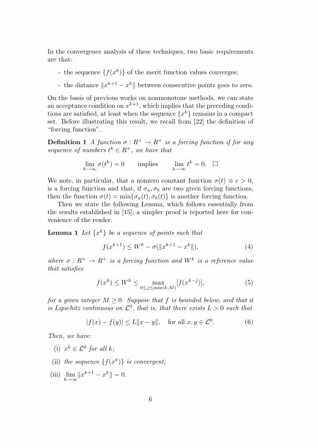
In the convergence analysis of these techniques, two basic requirementsare that:
- the sequence f(xk) of the merit function values converges;
- the distance ‖xk+1 − xk‖ between consecutive points goes to zero.
On the basis of previous works on nonmonotone methods, we can statean acceptance condition on xk+1, which implies that the preceding condi-tions are satisfied, at least when the sequence xk remains in a compactset. Before illustrating this result, we recall from [22] the definition of“forcing function”.
Definition 1 A function σ : R+ → R+ is a forcing function if for anysequence of numbers tk ∈ R+, we have that
limk→∞
σ(tk) = 0 implies limk→∞
tk = 0.
We note, in particular, that a nonzero constant function σ(t) ≡ c > 0,is a forcing function and that, if σa, σb are two given forcing functions,then the function σ(t) = minσa(t), σb(t) is another forcing function.
Then we state the following Lemma, which follows essentially fromthe results established in [15]; a simpler proof is reported here for con-venience of the reader.
Lemma 1 Let xk be a sequence of points such that
f(xk+1) ≤ W k − σ(‖xk+1 − xk‖), (4)
where σ : R+ → R+ is a forcing function and W k is a reference valuethat satisfies
f(xk) ≤ W k ≤ max0≤j≤min(k,M)
[f(xk−j)], (5)
for a given integer M ≥ 0. Suppose that f is bounded below, and that itis Lipschitz continuous on L0, that is, that there exists L > 0 such that
|f(x)− f(y)| ≤ L‖x− y‖, for all x, y ∈ L0. (6)
Then, we have:
(i) xk ∈ L0 for all k;
(ii) the sequence f(xk) is convergent;
(iii) limk→∞
‖xk+1 − xk‖ = 0.
6

Proof. For each k ≥ 0, let `(k) be an integer such that k−min(k, M) ≤`(k) ≤ k and that
f(x`(k)) = max0≤j≤min(k,M)
[f(xk−j)].
Then, (4) can be rewritten into the form:
f(xk+1) ≤ f(x`(k))− σ(‖xk+1 − xk‖). (7)
Noting that min(k + 1,M) ≤ min(k, M) + 1, we have:
f(x`(k+1)) = max0≤j≤min(k+1,M)
[f(xk+1−j)] ≤ max0≤j≤min(k,M)+1
[f(xk+1−j)]
= maxf(x`(k)), f(xk+1) = f(x`(k)),
where the last equality follows from (7). As f(x`(k) is nonincreasingand x`(0) = x0, it follows that f(xk) ≤ f(x0) for all k, so that thesequence xk belongs to the level set L0 and this proves assertion (i).Thus the nonincreasing sequence f(x`(k)) admits a limit for k →∞.Now, by induction on j, we show that at each k, for all j such that`(k) ≥ j ≥ 1, we have:
limk→∞
‖x`(k)−j+1 − x`(k)−j‖ = 0 (8)
andlim
k→∞f(x`(k)−j) = lim
k→∞f(x`(k)). (9)
If j = 1, using (7), where k is replaced by `(k)− 1, we can write
f(x`(k)) ≤ f(x`(`(k)−1))− σ(‖x`(k) − x`(k)−1‖
). (10)
Therefore, taking limits and recalling the definition of forcing function,it follows from (10) that
limk→∞
‖x`(k) − x`(k)−1‖ = 0. (11)
¿From (6) and (11) we obtain
limk→∞
f(x`(k)−1) = limk→∞
f(x`(k)),
so that (8) and (9) hold at each k for j = 1. Now assume that (9) holdsfor a given j. By (7) we can write
f(x`(k)−j) ≤ f(x`(`(k)−j−1))− σ(‖x`(k)−j − x`(k)−j−1‖
).
7
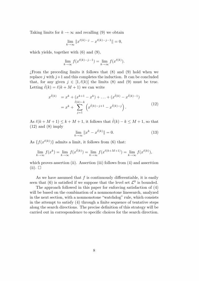
Taking limits for k →∞ and recalling (9) we obtain
limk→∞
‖x`(k)−j − x`(k)−j−1‖ = 0,
which yields, together with (6) and (9),
limk→∞
f(x`(k)−j−1) = limk→∞
f(x`(k)).
¿From the preceding limits it follows that (8) and (9) hold when wereplace j with j+1 and this completes the induction. It can be concludedthat, for any given j ∈ [1, `(k)] the limits (8) and (9) must be true.Letting ˆ(k) = `(k + M + 1) we can write
xˆ(k) = xk + (xk+1 − xk) + . . . + (xˆ(k) − x
ˆ(k)−1)
= xk +ˆ(k)−k∑
j=1
(x
ˆ(k)−j+1 − xˆ(k)−j
).
(12)
As `(k + M + 1) ≤ k + M + 1, it follows that ˆ(k)− k ≤ M + 1, so that(12) and (8) imply
limk→∞
‖xk − xˆ(k)‖ = 0. (13)
As f(x`(k)) admits a limit, it follows from (6) that:
limk→∞
f(xk) = limk→∞
f(xˆ(k)) = limk→∞
f(x`(k+M+1)) = limk→∞
f(x`(k)),
which proves assertion (ii). Assertion (iii) follows from (4) and asserttion(ii).
As we have assumed that f is continuously differentiable, it is easilyseen that (6) is satisfied if we suppose that the level set L0 is bounded.
The approach followed in this paper for enforcing satisfaction of (4)will be based on the combination of a nonmonotone linesearch, analyzedin the next section, with a nonmonotone “watchdog” rule, which consistsin the attempt to satisfy (4) through a finite sequence of tentative stepsalong the search directions. The precise definition of this strategy will becarried out in correspondence to specific choices for the search direction.
8

3 Nonmonotone derivative-free linesearches
In this section we describe nonmonotone linesearch techniques that canbe used for enforcing convergence of derivative-free methods for the min-imization of a differentiable merit function. We assume that for a sub-sequence of xk, the point xk+1 is generated through the iteration
xk+1 = xk + λkdk,
where dk ∈ Rn is a search direction and λk ∈ R is a stepsize. Theessential objective of a linesearch procedure is that of determining astepsize λk that guarantees a “sufficient reduction” of f , and it is also“sufficiently large” to satisfy the condition
limk→∞,k∈K
∇f(xk)T dk
‖dk‖ = 0,
whenever K is an infinite subset. In the computing schemes introducedhere, we also have to satisfy the condition
limk→∞
‖xk+1 − xk‖ = 0,
which has an important role in nonmonotone methods and in somederivative-free algorithms. A sufficient reduction of the objective func-tion values can be imposed by means of acceptability conditions ex-pressed in terms of a reference value W k, such that
f(xk) ≤ W k ≤ max0≤j≤min(k,M)
[f(xk−j)], (14)
where M is a given integer. In all the algorithms defined in this sectiona sufficient reduction of f will be guaranteed through conditions of theform:
f(xk + λkdk) ≤ W k − γ‖λkdk‖2, (15)
where γ > 0. When f(xk) converges, the same condition ensures that‖xk+1−xk‖ is forced to zero. As derivative information is not available,in order to satisfy (15) we must consider both positive and negativevalues for λ (or, equivalently, we must consider both the direction dk
and its opposite −dk). However, in the general case, we may have alsothat dk is orthogonal to∇f(xk) and hence we must impose a lower boundon the stepsize for detecting, at least asymptotically, this situation.
The linesearch schemes considered here can be distinguished, es-sentially, on the basis of the acceptance rules introduced for ensur-ing that the stepsize is “sufficiently large” to have, in the limit, that∇f(xk)T dk/‖dk‖ is driven to zero.
9

The simplest algorithm we introduce can be viewed as an Armijo-typetechnique, where, starting from an initial stepsize ak, we perform a searchalong the given direction dk and its opposite to ensure satisfaction of (15).The stepsize is reduced until either this condition is satisfied or the lengthof the tentative stepsize becomes smaller than a prefixed bound. In thelatter case, the stepsize determined by the algorithm is set equal to zeroand this corresponds, essentially, to a linesearch failure.An important requirement for defining this kind of scheme is that wecan compute a “sufficiently large” initial stepsize ak.
In derivative-based methods for general unconstrained optimizationproblems, it is known (see, e.g. [22] and [15] for the nonmonotone case)that this can be achieved, for instance, by imposing that there existssome forcing function σl such that
ak ≥ 1‖dk‖σl
(∇f(xk)T dk
‖dk‖)
.
In the no-derivative case, it might be difficult, in general, to imposeconditions related to the gradient of f . However, if a lower bound f∗
for the objective function value is known we can choose a sufficientlylarge initial stepsize, by relating ak to the f(xk) − f∗. In particular, ifwe assume that f is bounded below, we can set f∗ = 0 without loss ofgenerality, and we can impose a condition of the form
ak ≥ 1‖dk‖σl
(f(xk)
), (16)
for some forcing function σl. A special case of (16), which does notrequire an explicit knowledge of a lower bound, could be that of choosinga constant function as forcing function, by letting
ak ≥ c
‖dk‖ ,
for some c > 0. However, an obvious disadvantage of this criterion isthat the initial stepsize will be never accepted for k sufficiently large,because of the fact that the acceptability condition implies that
limk→∞
λk‖dk‖ = 0.
In the case of a system of nonlinear equations we can directly relate theinitial stepsize to the residual vector by requiring
ak ≥ 1‖dk‖σl
(‖F (xk)‖) . (17)
10

Assuming that a condition of the form (16) is imposed, we can definethe following algorithm.
Nonmonotone Derivative-Free Armijo-type LineSearch
(NDFALS) Algorithm
Data. dk ∈ Rn, dk 6= 0, W k defined as in (14), parameters
0 < θl < θu < 1, ρk ∈ (0, 1),
and a forcing function σl : R+ → R+.
Step 1. Choose ak such that
ak ≥ 1‖dk‖σl
(f(xk)
),
set λ = ak and ξ = ρk min1, ak, 1/‖dk‖.
Step 2. While f(xk ± λdk) > W k − γλ2‖dk‖2 do
If λ < ξ then
set λk = 0, ηk = λ and terminate,
else
choose θ ∈ [θl, θu] and set λ = θλ.End if
End while
Step 3. Let t ∈ −1, 1 be such that f(xk + tλdk) ≤ W k − γλ2‖dk‖2,set λk = tλ and terminate.
The properties of this scheme are summarized in the following two propo-sitions.
11

Proposition 1 Assume that f(x) ≥ 0 for all x ∈ Rn. Then algorithmNDFALS determines, in a finite number of iterations, a scalar λk suchthat
f(xk + λkdk) ≤ W k − γ(λk)2‖dk‖2, (18)
and at least one of the following conditions holds:
λk = 0 and f(xk±ηkdk) > fk−γ(ηk
)2 ‖dk‖2, (19)
with ηk < ρk min1, 1/‖dk‖ ,
0 < |λk| = ak (20)
0 < |λk| < ak and f(xk ± λk
θkdk) > fk − γ
(λk
θk
)2
‖dk‖2 (21)
with θk ∈ [θl, θu].
Proof. As λ is reduced by a factor
θ ≤ θu < 1
at each iteration, the algorithm terminates. either with λk = 0 or withλk 6= 0. In both cases, recalling that
fk ≤ W k,
it easily seen that λk satisfies the condition of sufficient reduction (18).
In the first case, taking into account the instructions of Step 1 and Step 2and the assumption fk ≤ W k, we have also that the scalar ηk computedat Step 2 must satisfy condition (19).
In the second case, termination occurs at Step 3 either with λk = ak, sothat (20) holds, or with |λk| < ak. In the latter case we have
f(xk ± λk
θkdk) > W k − γ
(λk
θk
)2
‖dk‖2 ≥ fk − γ
(λk
θk
)2
‖dk‖2,
for, otherwise, the initial stepsize would have not been reduced. It followsthat (21) holds. 2
12

Proposition 2 Assume that f(x) ≥ 0 for all x ∈ Rn. Let xk be asequence of points in Rn and let K be an infinite index set, such that
xk+1 = xk + λkdk,
for all k ∈ K, where dk ∈ Rn, dk 6= 0 and λk ∈ R is determined bymeans of Algorithm NDFALS.Assume that ρk → 0 for k →∞, k ∈ K. Suppose that the sequence fkconverges and that the subsequence xkK is bounded. Then, we have
limk→∞,k∈K
∇f(xk)T dk
‖dk‖ = 0.
Proof. If the assertion is false, we can find an infinite subset K1 ⊆ Ksuch that
limk→∞,k∈K1
xk = x,
and
limk→∞,k∈K1
∇f(xk)T dk
‖dk‖ = ∇f(x)T d 6= 0. (22)
As the sequences xkK and dk/‖dk‖ are bounded, the continuityassumption on ∇f ensures the existence of a subsequence that yieldsthe preceding limit.We can also assume that
f(x) 6= 0, (23)
for, otherwise, x would be an unconstrained minimizer of f ≥ 0 andhence would satisfy the stationary condition ∇f(x) = 0. By Proposition1 we know that algorithm NDFALS terminates for each k and satisfiesthe conditions stated there. Assume first that there exists a k ∈ K1 suchthat, for all k ∈ K1 and k ≥ k, Algorithm NDFALS terminates at Step2 with λk = 0 and determines ηk > 0 such that,
ηk < ρk min1, 1/‖dk‖ (24)
and (19) is satisfied. From (19), using the Mean Value Theorem, itfollows that there exist points uk = xk + ζkηkdk and vk = xk − βkηkdk
with ζk, βk ∈ (0, 1), such that
∇f(uk)T dk
‖dk‖ > −γηk‖dk‖. (25)
and∇f(vk)T dk
‖dk‖ < γηk‖dk‖. (26)
13

Recalling (24) and the assumption that ρk → 0 for k →∞ and k ∈ K1,we have that uk → x and vk → x for k → ∞ and k ∈ K1, and hence,taking limits and recalling that dk/‖dk‖k1 converges to d, we obtain∇f(x)T d = 0, which contradicts (22). Therefore, we can suppose thatthere exists an infinite subset K2 ⊆ K1 such that, for all k ∈ K2, wecompute λk 6= 0, such that
f(xk + λkdk) ≤ W k − γ(λk)2‖dk‖2, (27)
and one of the conditions (20), (21) is satisfied. By assumption, we havethat fk converges to a limit, so that, by the assumptions on W k, alsothe sequence W k converges to the same limit. Then, from (27) we get
limk→∞,k∈K2
λk‖dk‖ = 0. (28)
Now, if (21) holds for an infinite subsequence, we can use again the MeanValue Theorem and we can repeat reasonings similar to that followed inthe case λk = 0 (with λk/θk replacing ηk), thus obtaining in the limitthat ∇f(x)T d = 0, which contradicts (22). Finally, we suppose that forsufficiently large k ∈ K3 with K3 ⊆ K1, we have that λk = ak. In thiscase, it follows from (28) and the instructions of Algorithm NDFALSthat
limk→∞,k∈K3
σl
(‖f(xk)‖) = 0,
which implies f(x) = 0, and this contradicts (23). 2
A possible disadvantage of Algorithm NDFALS could be that the forc-ing function σl appearing in condition (16) must be specified in advance.Moreover, in case of general unconstrained minimization problems, wemust assume the knowledge of a lower bound for f , or tolerate an ineffi-cient choice of the initial stepsize. In order to overcome these limitations,we introduce here a different scheme that can be used, in principle, in theunconstrained minimization of any continuously differentiable functionand it can be employed using any initial (variable) tentative stepsize ak.The main difference with respect to the Armijo-type scheme definedabove is that, when ak satisfies the condition of sufficient reduction,then an appropriate sign of λk is chosen and the stepsize is possiblyincreased, until (derivative-free) Goldstein-type conditions are satisfied,or a larger tentative stepsize violates a condition of sufficient decrease.
A conceptual model of the algorithm is defined in the following scheme.
14

Nonmonotone Derivative-Free LineSearch (NDFLS) Algorithm
Data. dk ∈ Rn, dk 6= 0, W k defined as in (14), and parameters
0 < θl < θu < 1, 1 < µl < µu, γ1 > γ > 0, ak > 0, ρk ∈ (0, 1).
Step 1. Set λ = ak and ξ = ρk min1, ak, 1/‖dk‖.
Step 2. While f(xk ± λdk) > W k − γλ2‖dk‖2 do
If λ‖dk‖ < ξ then
set λk = 0, ηk = λ and terminate,
else
choose θ ∈ [θl, θu] and set λ = θλ.End if
End while
Step 3. Let t ∈ −1, 1 be such that f(xk + tλdk) ≤ W k − γλ2‖dk‖2and set λ = tλ.
Step 4. If |λ| < ak, then set λk = λ and terminate.
Step 5. If f(xk ± λdk) ≥ fk, then set λk = λ and terminate.
Step 6. Let s ∈ −1, 1 be such that f(xk + sλdk) < fk, set λ = sλand choose µ ∈ [µl, µu].
Step 7. While
f(xk + λdk) < fk − γ1λ2‖dk‖2
and
f(xk + µλdk) < minf(xk + λdk), fk − γ (µλ)2 ‖dk‖2
. set λ = µλ and choose µ ∈ [µl, µu].
End while
Step 8. Set λk = λ and terminate.
We show first that Algorithm NDFLS is well defined.
15

Proposition 3 Assume that f is bounded below on Rn. Then AlgorithmNDFLS determines, in a finite number of iterations, a scalar λk such that
f(xk + λkdk) ≤ W k − γ(λk)2‖dk‖2, (29)
and at least one of the following conditions holds:
λk = 0 and f(xk±ηkdk) > fk−γ(ηk
)2 ‖dk‖2,(30)
with ηk < ρk min1, 1/‖dk‖.
λk 6= 0 and f(xk±λk
θkdk) > fk−γ
(λk
θk
)2
‖dk‖2, (31)
with θk ∈ [θl, θu]
λk 6= 0 and f(xk±λkdk) ≥ fk
(32)λk 6= 0 and f(xk + λkdk) ≥ fk − γ1
(λk
)2 ‖dk‖2,(33)
with f(xk + λkdk) < fk
λk 6= 0 and f(xk + µkλkdk) ≥ minf(xk + λkdk), fk − γ(µkλk
)2 ‖dk‖2(34)
with f(xk + λkdk) < fk and 1 < µl ≤ µk ≤ µu.
Proof. In order to prove that the algorithm terminates we must showthat, for each k, it does not cycle infinitely at Step 2 or at Step 7. Thealgorithm cannot cycle infinitely at Step 2, since λ is reduced by a factorθ ≤ θu < 1 at each iteration. The cycle at Step 7 must terminate since,on the contrary, letting h be a counter of the iterations of the cycle, weshould have, in particular:
f(xk + λ(h)dk) < fk − γ1λ(h)2‖dk‖2
for some infinite sequence λ(h) such that |λ(h)| → ∞ for h →∞, butthis contradicts the assumption that f is bounded below. It follows thatthe algorithm terminates either with λk = 0 or with λk 6= 0. In bothcases, recalling that fk ≤ W k, it easily seen that λk satisfies the con-dition of sufficient reduction (29). In the first case, taking into accountthe instructions of Step 1 and Step 2 and the assumption fk ≤ W k, wehave also that the scalar ηk computed at Step 3 must satisfy (30).
16

In the second case, termination may occur at Step 4, at Step 5 or atStep 8. If the algorithm terminates at Step 4, then we have
f(xk ± λk
θkdk) > W k − γ
(λk
θk
)2
‖dk‖2 ≥ fk − γ
(λk
θk
)2
‖dk‖2,
for, otherwise, the initial stepsize ak would have not been reduced, andtherefore condition (31) must be true. If the algorithm terminates atStep 5 we have obviously that (32) is satisfied. Finally, assume thatthe algorithm terminates at Step 8. We can observe that, because of theinstructions at Step 5 and 6, the cycle is started only when f(xk+λdk) <fk and subsequently the instructions at Step 7 ensure that f is strictlydecreasing for increasing values of |λ|, since we must have, in particular,that f(xk + µλdk) < f(xk + λdk). Thus, if termination occurs at Step 8we have necessarily f(xk+λkdk) < fk. Taking this into account, it easilyseen that one of the inequalities (33) (34) must hold at termination. 2
The next proposition establishes the convergence properties of AlgorithmNDFLS.
Proposition 4 Assume that f is bounded below on Rn. Let xk be asequence of points in Rn and let K be an infinite index set, such that
xk+1 = xk + λkdk,
for all k ∈ K, where dk ∈ Rn, dk 6= 0 and λk ∈ R is determined bymeans of Algorithm NDFLS.Assume that ρk → 0 for k → ∞, k ∈ K. Then, if the sequence fkconverges and the subsequence xkK is bounded, we have
limk→∞,k∈K
∇f(xk)T dk
‖dk‖ = 0.
Proof. Reasoning by contradiction, assume there exists an infinite sub-set K1 ⊆ K such that
limk→∞,k∈K1
xk = x
and
limk→∞,k∈K1
∇f(xk)T dk
‖dk‖ = ∇f(x)T d 6= 0. (35)
As the sequences xkK and dk/‖dk‖ are bounded, the continuityassumption on ∇f ensures the existence of a subsequence that yields thepreceding limits. Moreover, by Proposition 3 we know that algorithmNDFLS terminates for each k and satisfies the conditions stated there.
17

Assume first that there exists a k ∈ K1 such that, for all k ∈ K1 andk ≥ k, Algorithm NDFLS terminates at Step 3 with λk = 0. In thiscase we can reason as in the proof of Proposition 2, thus obtaining acontradiction to (35).
Now suppose that there exists an infinite subset K2 ⊆ K1 such that,for all k ∈ K2, we compute λk 6= 0, such that
f(xk + λkdk) ≤ W k − γ(λk)2‖dk‖2, (36)
and one of the conditions (31), (32), (33), (34) is satisfied. As fkconverges we get
limk→∞,k∈K2
λk‖dk‖ = 0. (37)
Now, we can use again (appropriately) the Mean Value Theorem, incorrespondence to each pair of inequalities that bound the variations off in the conditions (31), (32), (33), (34). We observe only that when(34) is valid and we have, in particular, that
f(xk + µkλkdk) ≥ f(xk + λkdk),
then the Mean Value Theorem can be used in this inequality, by writing
f(xk + µkλkdk) = f(xk + λkdk + (µk − 1)λkdk)
= f(xk + λkdk) + (µk − 1)λk∇f(zk)T dk,
wherezk := xk + λkdk + ξk(µk − 1)λkdk,
for some ξk ∈ (0, 1). As dk 6= 0, this implies that
∇f(zk)T dk
‖dk‖ ≥ 0.
Taking into account (37), we can repeat for each of the conditions (31-34) reasonings similar to that followed in the proof of Proposition 2,obtaining in the limit (for some subsequence, if necessary) that
∇f(x)T d = 0,
which contradicts (35). 2
Under additional regularity assumptions on ∇f we can give an explicitestimate of a lower bound for the stepsizes produced by Algorithm ND-FLS. More specifically, we can state the following result.
18
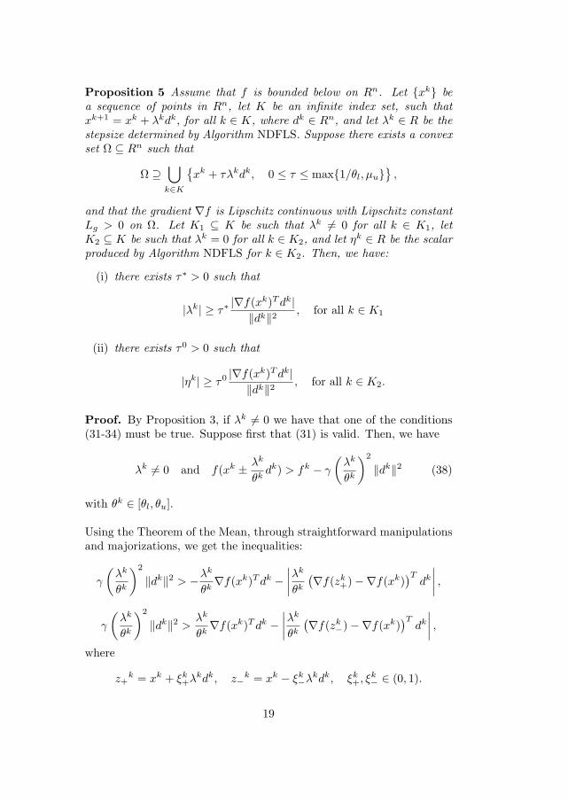
Proposition 5 Assume that f is bounded below on Rn. Let xk bea sequence of points in Rn, let K be an infinite index set, such thatxk+1 = xk + λkdk, for all k ∈ K, where dk ∈ Rn, and let λk ∈ R be thestepsize determined by Algorithm NDFLS. Suppose there exists a convexset Ω ⊆ Rn such that
Ω ⊇⋃
k∈K
xk + τλkdk, 0 ≤ τ ≤ max1/θl, µu
,
and that the gradient ∇f is Lipschitz continuous with Lipschitz constantLg > 0 on Ω. Let K1 ⊆ K be such that λk 6= 0 for all k ∈ K1, letK2 ⊆ K be such that λk = 0 for all k ∈ K2, and let ηk ∈ R be the scalarproduced by Algorithm NDFLS for k ∈ K2. Then, we have:
(i) there exists τ∗ > 0 such that
|λk| ≥ τ∗|∇f(xk)T dk|
‖dk‖2 , for all k ∈ K1
(ii) there exists τ0 > 0 such that
|ηk| ≥ τ0 |∇f(xk)T dk|‖dk‖2 , for all k ∈ K2.
Proof. By Proposition 3, if λk 6= 0 we have that one of the conditions(31-34) must be true. Suppose first that (31) is valid. Then, we have
λk 6= 0 and f(xk ± λk
θkdk) > fk − γ
(λk
θk
)2
‖dk‖2 (38)
with θk ∈ [θl, θu].
Using the Theorem of the Mean, through straightforward manipulationsand majorizations, we get the inequalities:
γ
(λk
θk
)2
‖dk‖2 > −λk
θk∇f(xk)T dk −
∣∣∣∣λk
θk
(∇f(zk+)−∇f(xk)
)Tdk
∣∣∣∣ ,
γ
(λk
θk
)2
‖dk‖2 >λk
θk∇f(xk)T dk −
∣∣∣∣λk
θk
(∇f(zk−)−∇f(xk)
)Tdk
∣∣∣∣ ,
where
z+k = xk + ξk
+λkdk, z−k = xk − ξk−λkdk, ξk
+, ξk− ∈ (0, 1).
19
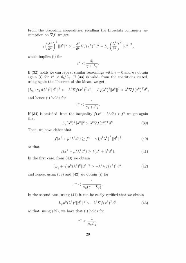
From the preceding inequalities, recalling the Lipschitz continuity as-sumption on ∇f , we get
γ
(λk
θk
)2
‖dk‖2 > ±λk
θk∇f(xk)T dk − Lg
(λk
θk
)2 ∥∥dk∥∥2
,
which implies (i) for
τ∗ <θl
γ + Lg.
If (32) holds we can repeat similar reasonings with γ = 0 and we obtainagain (i) for τ∗ < θl/Lg. If (33) is valid, from the conditions stated,using again the Theorem of the Mean, we get:
(Lg+γ1)(λk)2‖dk‖2 > −λk∇f(xk)T dk, Lg(λk)2‖dk‖2 > λk∇f(xk)T dk,
and hence (i) holds for
τ∗ <1
γ1 + Lg.
If (34) is satisfied, from the inequality f(xk + λkdk) < fk we get againthat
Lg(λk)2‖dk‖2 > λk∇f(xk)T dk. (39)
Then, we have either that
f(xk + µkλkdk) ≥ fk − γ(µkλk
)2 ‖dk‖2 (40)
or thatf(xk + µkλkdk) ≥ f(xk + λkdk). (41)
In the first case, from (40) we obtain
(Lg + γ)µk(λk)2‖dk‖2 > −λk∇f(xk)T dk, (42)
and hence, using (39) and (42) we obtain (i) for
τ∗ <1
µu(γ + Lg).
In the second case, using (41) it can be easily verified that we obtain
Lgµk(λk)2‖dk‖2 > −λk∇f(xk)T dk, (43)
so that, using (39), we have that (i) holds for
τ∗ <1
µuLg.
20

It can be concluded that (i) holds for k ∈ K1, provided that
0 < τ∗ < min
θl
γ + Lg,
1γ1 + Lg
,1
µu(γ + Lg)
.
Now suppose that k ∈ K2, so that (30) is valid. Using the same kindof arguments employed above, we can easily establish that (ii) is true,provided that
τ0 <θl
γ + Lg.
We note that Proposition 5 above yields also another direct proof ofProposition 4, if we add the Lipschitz continuity assumption on ∇fin the statement of this proposition. In fact, since both ηk‖dk‖ andλk‖dk‖ go to zero, because of the instructions of Algorithm NDFLS andthe convergence of fk, the assertion of Proposition 4 is an immediateconsequence of (i) and (ii) of Proposition 5.
In the sequel we will refer to Algorithm NDFLS as to a procedure,with input parameters (x, d, ρ) and output λ, indicated with NDFLS(x, d,ρ, λ). For all k, the initial tentative stepsize along dk may depend on thespecific choice of dk.
4 Global stabilization of a residual-basedalgorithm
In this section we define a nonmonotone globalization scheme for aderivative-free algorithm employing the residual vector as search direc-tion. Moreover, we present a specific version of the algorithm where, asproposed in [18], the Barzilai-Borwein (BB) method is used for comput-ing a suitable scaling factor of the residual vector. We refer to the meritfunction f : Rn → R, defined as
f(x) =12‖F (x)‖2, (44)
where ‖ · ‖ is the Euclidean norm on Rn.The stabilization strategy is based on the combination of nonmono-
tone watchdog rules with the nonmonotone derivative-free linesearch Al-gorithm NDFLS presented in Section 3. The algorithm can be defined interms of a sequence of major iterations, where a finite sets of tentativepoints is generated using the possibly scaled residual vectors.
21

More specifically, at any major iteration k, starting from the currentpoint xk and letting z0 = xk, the tentative points zi+1 are generatedusing the iteration
zi+1 = zi − 1αi
F (zi),
where i ∈ 0, . . . , N − 1 and αi is such that
0 < ` ≤ |αi| ≤ u, (45)
for some given u > ` > 0. A tentative point is accepted as the new iter-ate xk+1, whenever a nonmonotone watchdog test, which measures theactual reduction of the objective function with respect to some referencevalue, is satisfied. In particular, the acceptance condition on zi+1 canbe expressed in the form
f(zi+1) ≤ V k −maxσ1
(‖zi+1 − xk‖) , σ2
(‖F (xk)‖), (46)
where V k is a reference value satisfying
f(xk) ≤ V k ≤ max0≤j≤min(k,M)
[f(xk−j)], (47)
where M ≥ 0 is a prefixed integer, and σ1, σ2 are given forcing functions.Note that the reference value V k can be different from that used inAlgorithm NDFLS and denoted by W k.
If (46) is satisfied at some i, then we set
xk+1 = zi+1
and hence we have that
f(xk+1) ≤ V k −maxσ1
(‖xk+1 − xk‖) , σ2
(‖F (xk)‖). (48)
This implies in particular that condition (4) of Lemma 1 is satisfied at xk.We will show in the sequel that the existence of an infinite subsequencesatisfying (48) is sufficient to prove that
limk→∞
F (xk) = 0.
When no tentative point is accepted during a prefixed number of steps,we backtrack to xk and compute a stepsize along a suitable directiondk, through the nonmonotone derivative-free algorithm of the precedingsection.
As stopping rule we require, in the convergence analysis, that F (xk) =0. A conceptual algorithm model is reported below.
22
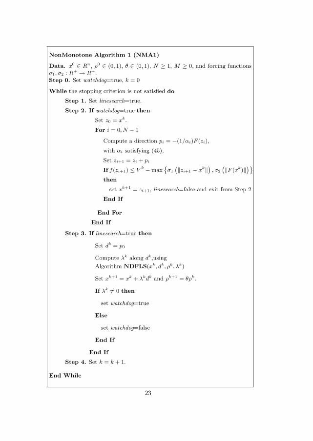
NonMonotone Algorithm 1 (NMA1)
Data. x0 ∈ Rn, ρ0 ∈ (0, 1), θ ∈ (0, 1), N ≥ 1, M ≥ 0, and forcing functionsσ1, σ2 : R+ → R+.Step 0. Set watchdog=true, k = 0
While the stopping criterion is not satisfied do
Step 1. Set linesearch=true.
Step 2. If watchdog=true then
Set z0 = xk.
For i = 0, N − 1
Compute a direction pi = −(1/αi)F (zi),
with αi satisfying (45),
Set zi+1 = zi + pi
If f(zi+1) ≤ V k −maxσ1
(‖zi+1 − xk‖
), σ2
(‖F (xk)‖
)
then
set xk+1 = zi+1, linesearch=false and exit from Step 2
End If
End For
End If
Step 3. If linesearch=true then
Set dk = p0
Compute λk along dk,using
Algorithm NDFLS(xk, dk, ρk, λk)
Set xk+1 = xk + λkdk and ρk+1 = θρk.
If λk 6= 0 then
set watchdog=true
Else
set watchdog=false
End If
End If
Step 4. Set k = k + 1.
End While
23
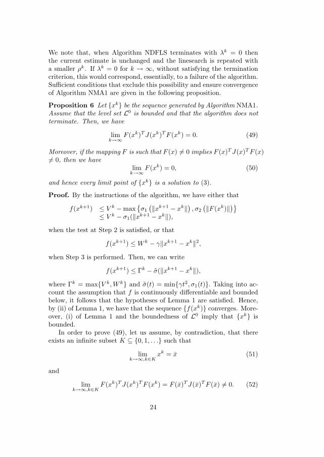
We note that, when Algorithm NDFLS terminates with λk = 0 thenthe current estimate is unchanged and the linesearch is repeated witha smaller ρk. If λk = 0 for k → ∞, without satisfying the terminationcriterion, this would correspond, essentially, to a failure of the algorithm.Sufficient conditions that exclude this possibility and ensure convergenceof Algorithm NMA1 are given in the following proposition.
Proposition 6 Let xk be the sequence generated by Algorithm NMA1.Assume that the level set L0 is bounded and that the algorithm does notterminate. Then, we have
limk→∞
F (xk)T J(xk)T F (xk) = 0. (49)
Moreover, if the mapping F is such that F (x) 6= 0 implies F (x)T J(x)T F (x)6= 0, then we have
limk→∞
F (xk) = 0, (50)
and hence every limit point of xk is a solution to (3).
Proof. By the instructions of the algorithm, we have either that
f(xk+1) ≤ V k −maxσ1
(‖xk+1 − xk‖) , σ2
(‖F (xk)‖)≤ V k − σ1(‖xk+1 − xk‖),
when the test at Step 2 is satisfied, or that
f(xk+1) ≤ W k − γ‖xk+1 − xk‖2,when Step 3 is performed. Then, we can write
f(xk+1) ≤ Γk − σ(‖xk+1 − xk‖),where Γk = maxV k,W k and σ(t) = minγt2, σ1(t). Taking into ac-count the assumption that f is continuously differentiable and boundedbelow, it follows that the hypotheses of Lemma 1 are satisfied. Hence,by (ii) of Lemma 1, we have that the sequence f(xk) converges. More-over, (i) of Lemma 1 and the boundedness of L0 imply that xk isbounded.
In order to prove (49), let us assume, by contradiction, that thereexists an infinite subset K ⊆ 0, 1, . . . such that
limk→∞,k∈K
xk = x (51)
and
limk→∞,k∈K
F (xk)T J(xk)T F (xk) = F (x)T J(x)T F (x) 6= 0. (52)
24
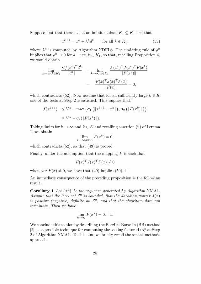
Suppose first that there exists an infinite subset K1 ⊆ K such that
xk+1 = xk + λkdk for all k ∈ K1, (53)
where λk is computed by Algorithm NDFLS. The updating rule of ρk
implies that ρk → 0 for k →∞, k ∈ K1, so that, recalling Proposition 4,we would obtain
limk→∞,k∈K1
∇f(xk)T dk
‖dk‖ = limk→∞,k∈K1
F (xk)T J(xk)T F (xk)‖F (xk)‖
=F (x)T J(x)T F (x)
‖F (x)‖ = 0,
which contradicts (52). Now assume that for all sufficiently large k ∈ Kone of the tests at Step 2 is satisfied. This implies that:
f(xk+1) ≤ V k −maxσ1
(‖xk+1 − xk‖) , σ2
(‖F (xk)‖)
≤ V k − σ2(‖F (xk)‖).Taking limits for k →∞ and k ∈ K and recalling assertion (ii) of Lemma1, we obtain
limk→∞,k∈K
F (xk) = 0,
which contradicts (52), so that (49) is proved.
Finally, under the assumption that the mapping F is such that
F (x)T J(x)T F (x) 6= 0
whenever F (x) 6= 0, we have that (49) implies (50).
An immediate consequence of the preceding proposition is the followingresult.
Corollary 1 Let xk be the sequence generated by Algorithm NMA1.Assume that the level set L0 is bounded, that the Jacobian matrix J(x)is positive (negative) definite on L0, and that the algorithm does notterminate. Then we have
limk→∞
F (xk) = 0.
We conclude this section by describing the Barzilai-Borwein (BB) method[2], as a possible technique for computing the scaling factors 1/αk
i at Step2 of Algorithm NMA1. To this aim, we briefly recall the secant-methodsapproach.
25

Let x+, x− be given points, and let F (x+) and F (x−) be the correspond-ing residual vectors. In the secant methods, the Jacobian matrix J(x+)is approximated by a suitable matrix A+ satisfying the secant equation
A+s = y, (54)
wheres = x+ − x−,
andy = F (x+)− F (x−).
The existing methods differ in the choice of the matrix A+, since (54)does not uniquely specify A+. In the BB method, the Jacobian matrixJ(x+) is approximated by
A+ ≡ α(a)+ I,
or J(x+)−1 is approximated by
A−1+ ≡ (1/α
(b)+ )I,
where the scalars α(a)+ and α
(b)+ are obtained by minimizing with respect
to α the quantities‖αs− y‖,
and‖s− 1
αy‖,
which represent the errors on the secant equation. This leads to the BBformulae
α(a)+ =
sT y
sT s(55)
α(b)+ =
yT y
sT y, (56)
which can be adopted for defining the search direction pki , at Step 2 of
Algorithm NMA1.
More specifically, letting
z−1 = xk−1, for k ≥ 1,
the tentative points zi+1 are generated using the iteration
zi+1 = zi − 1αi
F (zi),
26

where αi is defined either by αi = sT y/sT s, or by αi = yT y/sT y, with
s = zi − zi−1
andy = F (zi)− F (zi−1).
The value computed through one of the preceding formulae is (possibly)modified in a way that condition (45) holds. Further implementationaspects of the version of Algorithm NMA1 using the BB scaling rule willbe discussed in Section 6.
5 Hybrid algorithm employing linearly in-dependent directions
In this section we consider a hybrid algorithm, in which the residualbased algorithm of the preceding section is combined with linesearchesalong a set of linearly independent directions, in order to enforce con-vergence towards stationary points of the merit function
f(x) = 1/2‖F (x)‖2.
More specifically, at each iteration k, a set of tentative points is gen-erated as in Algorithm NMA1 and the current point is accepted if thenonmonotone watchdog test is satisfied. When no tentative point is ac-cepted during a prefixed number of N steps, we first compute a stepsizeλ through a nonmonotone linesearch along the direction
d = −F (xk)/α0.
However, in contrast to the strategy of Algorithm NMA1, we accept thenew point
x = xk + λd
as the next iterate xk+1, only when the stepsize |λ| satisfies a suitabletest, related to the estimated size of the residual. When this test isnot satisfied, a set of new iterates is determined through a (possibly fi-nite) sequence of derivative-free linesearches, along directions extractedsequentially from a given set q1, . . . , qn of n linearly independent vec-tors, which can be identified, for instance, with the set of coordinatedirections.
27

If a non zero stepsize is obtained during this phase, which will be in-dicated as the coordinate phase, then the algorithm switches again toresidual-based steps employing the BB formulae and a new major itera-tion is started.
The acceptance test on the results of the linesearch along d has theobjective of avoiding, as much as possible, the use of the search directionsqi, which can be expensive in case of large-dimensional systems, whileguaranteeing that a stationary point of f will be located in the limit.To this aim, first we define an estimate of the smallest residual currentlyavailable, by setting
rk = min‖F (xk + λd)‖, min
0≤j≤k‖F (xj)‖
, (57)
Then, if λ 6= 0, we introduce the following conditions, where br > 0 andcr > 0 are given numbers:
|λ| ≥ minbr, rk, (58)
1‖d‖
∣∣∣∣∣f(xk + λd)− f(xk)
λ
∣∣∣∣∣ ≥ crrk. (59)
It will be shown that, if λ 6= 0 and one of conditions (58) (59) is satis-fied for all k, then the coordinate phase may be not performed and yetconvergence towards stationary points of f can be established.
When λ = 0 or when both conditions (58) and (59) are violated, wemust start the coordinate phase and select one of the vectors qi.
Under the assumption that the Jacobian matrix is non singular, wewill prove that, using these rules, the limit points of the sequence xkwill be stationary points of f , provided that all the directions in the setq1, . . . , qn are considered sufficiently often.
A formal description of the hybrid algorithm that incorporates the pre-ceding criteria is reported below. We assume that V k is a reference valuesatisfying (47) and that all linesearches are performed through AlgorithmNDFLS.
In the application of the linesearch procedure we assume that theinitial stepsize ak is the unit stepsize along d, but we admit any othermore convenient choice along the search directions qi. The stoppingcriterion is again the condition that F (xk) = 0.
28

NonMonotone Algorithm 2 (NMA2)
Data. x0 ∈ Rn, br, cr > 0, ρ0, θ ∈ (0, 1), N ≥ 1, M ≥ 0, k = 0, j0 = 1,
and forcing functions σ1, σ2 : R+ → R+.
While the stopping criterion is not satisfied do
Step 1. Set linesearch=true, coord=true , z0 = xk.
Step 2. For i = 0, N − 1
Compute pi = −(1/αi)F (zi), with αi satisfying (45)
and set zi+1 = zi + pi
If f(zi+1) ≤ V k −maxσ1
(‖zi+1 − xk‖
), σ2
(‖F (xk)‖
)
then
set xk+1 = zi+1, k = k + 1, linesearch=false
and exit from Step 2
End If
End For
Step 3. If linesearch=true then
set d = p0, compute the stepsize λ by means of
Algorithm NDFLS (xk, d, ρk, λ)
If λ 6= 0 and one of the conditions (58) or (59) is satisfied
then
set λk = λ, dk = d, ρk+1 = θρk, xk+1 = xk + λkdk,
k = k + 1 and coord=false
Else
set t = jk, coord=true.
End if
While coord=true
Compute the stepsize λ by means of
Algorithm NDFLS(xk, qt, ρk, λ)
set λk = λ, dk = qt, xk+1 = xk + λkdk, ρk+1 = θρk
and k = k + 1
If λ 6= 0 then set coord=false end if
End While
End If
End While
29

The convergence of Algorithm NMA2 is established in the next propo-sition.
Proposition 7 Let xk be the sequence generated by Algorithm NMA2.Assume that the level set L0 is bounded and that the Jacobian matrixJ(x) is nonsingular on L0. Then, if the algorithm does not terminatewe have
limk→∞
F (xk) = 0, (60)
and hence every limit point of xk is a solution to (3).
Proof. The instructions of the algorithm imply that each point xk+1
is obtained either as a result of the watchdog test, or because of thefact that the acceptance conditions of Algorithm NDFLS are satisfied.Using the same reasonings employed in the proof of Proposition 6, andrecalling Lemma 1, we can assert that xk belongs to the compact set L0
for all k, that the sequence f(xk) converges to some limit f∗, that is:
limk→∞
f(xk) = limk→∞
12‖F (xk)‖ = f∗, (61)
and that there holds the limit
limk→∞
‖xk+1 − xk‖ = 0. (62)
We note preliminarily that assertion (60) can be established by prov-ing that, for some subsequence, we have either that f(xk) → 0 or that∇f(xk) → 0. In fact, in the first case, by (61) we have that the wholesequence ‖F (xk)‖ converges to zero. In the second case, by the com-pactness assumption on L0, we can find a subsequence of xkK con-verging to some x, so that ∇F (x) = J(x)T F (x) = 0 and hence, as J isnon singular, we get F (x) = 0. Thus we have again that f(xk) → 0 fora subsequence, which implies, as noted above, that (60) must be true.
Now, suppose first that there exists an infinite subset K1 such thatStep 3 is never performed for all k ∈ K1, because of the fact that one ofthe acceptance conditions at Step 2 is satisfied. This implies that:
f(xk+1) ≤ V k −maxσ1
(‖xk+1 − xk‖) , σ2
(‖F (xk)‖)
≤ V k − σ2(‖F (xk)‖).
Taking limits for k →∞ and k ∈ K1, we obtain
limk→∞,k∈K1
‖F (xk)‖ = 0.
30

As remarked earlier, this establishes the thesis and hence we can restrictour attention to the case where Step 3 is performed for all sufficientlylarge k. In this case, a first possibility is that, for some infinite subse-quence, one of the conditions (58) or (59) is satisfied, so that we can findxkK2 converging to some x such that, for k ∈ K2, we have:
λk = λ, dk = d = −F (xk)/αk0 , xk+1 = xk + λkdk
andrk = min
0≤j≤k+1‖F (xj)‖ = ||F (xjk)||,
where xjk , with 0 ≤ jk ≤ k + 1, is a point where the above minimum isattained.
Now, if (58) holds for an infinite subsequence, say for k ∈ K3 withK3 ⊆ K2, multiplying both members of (58) by ‖dk‖, we can write
|λk|‖dk‖ ≥ ‖dk‖minbr, rk =
‖F (xk)‖|αk
0 |minbr, ||F (xjk)||, k ∈ K3.
Then, taking limits for k → ∞, k ∈ K3, by (62) we have either that‖F (xk)‖/αk
0 → 0 for any infinite subsequence, or else that we can extractan infinite subsequence of points xjk such that ||F (xjk)|| → 0. Recalling(45), in both cases we can assert that ‖F (xk)‖ → 0 for some subsequence,which establishes the thesis.
Assume now that (59) holds for an infinite subsequence, say for k ∈ K4
with K4 ⊆ K2, so that we can write:
1‖dk‖
∣∣∣∣f(xk + λkdk)− f(xk)
λk
∣∣∣∣ ≥ cr||F (xjk)||, k ∈ K4. (63)
Using the Theorem of the Mean, from (63) we get
|∇f(zk)T dk|‖dk‖ ≥ cr||F (xjk)||, k ∈ K4, (64)
wherezk = xk + ξkλkdk, ξk ∈ (0, 1).
As xk is bounded, there must exist an infinite subset K5 ⊆ K4 andvectors x, d ∈ Rn such that
limk→∞,k∈K5
xk = x, limk→∞,k∈K5
dk
‖dk‖ = d. (65)
31

Moreover, as λk is computed through Algorithm NDFLS and the up-dating rule for ρk implies that ρk → 0 for k → ∞, by Proposition 4,equations (65) and the continuity assumptions, we get
limk→∞,k∈K5
∇f(xk)T dk
‖dk‖ = ∇f(x)T d = 0. (66)
On the other hand, taking limits for k →∞, k ∈ K5 and using (62), wehave that zk → x, so that (66) implies:
limk→∞,k∈K5
|∇f(zk)T dk|‖dk‖ = ∇f(x)T d = 0. (67)
Therefore, from (64) it follows that
limk→∞,k∈K5
||F (xjk)|| = 0,
and hence we have again that F (xk) → 0 for some subsequence, whichproves our thesis.
Finally, we can assume that for all sufficiently large k the points ofthe sequence are generated only during the while cycle at Step 3, usingAlgorithm NDFLS for computing the stepsize λk (possibly zero) alongthe search directions qi. As all these directions are used sequentially, itfollows that
dk+1, . . . , dk+n = q1, . . . , qn,and hence, by Proposition 4 we can write
limk→∞
∇f(xk+i)T dk+i
‖dk+i‖ = 0 i = 1, . . . , n. (68)
Now, by the compactness assumption on L0 and (62), there must existsome subsequence xkK , such that
limk→∞,k∈K
xk+i = x i = 1, . . . , n (69)
and hence, as dk+1, . . . , dk+n = q1, . . . , qn, by (68) and (69) weobtain
∇f(x)T qi = 0 i = 1, . . . , n,
which, recalling the linear independence of q1, . . . , qn, implies∇f(x) = 0.This completes the proof.
32

When the Jacobian matrix is definite on L0 we can show that the accep-tance test at Step 3 on λ is automatically satisfied for sufficiently largek and hence the coordinate search phase is ultimately skipped. Beforestating this result we recall a sufficient condition for ∇f to be Lipschitzcontinuous on a given set Ω, when we assume f(x) = 1/2‖F (x)‖2.Proposition 8 Suppose that J is Lipschitz continuous, with Lipschitzconstant Lj, on a convex set Ω ⊆ Rn and that there exist mF > 0 andmJ > 0 such that ‖F (x)‖ ≤ mF and ‖J(x)‖ ≤ mJ for all x ∈ Ω. Then,if f(x) = 1/2‖F (x)‖2, we have that ∇f(x) = J(x)T F (x) is Lipschitzcontinuous on Ω.
Proof. We recall ([22], Corollary 3.24) that, under the assumptionstated, F is also Lipschitz continuous on Ω and hence there exists LF
such that‖F (x)− F (y)‖ ≤ LF ‖x− y‖,
for all x, y ∈ Ω. Then we must only note that
‖∇f(x)−∇f(y)‖ = ‖J(x)T F (x)− J(y)T F (y)‖
= ‖(J(x)− J(y))T F (x) + J(y)T (F (x)− F (y))‖
≤ ‖J(x)− J(y)‖‖F (x)‖+ ‖J(y)‖F (x)− F (y)‖
≤ (LJmF + mJLF )‖x− y‖.Now, assuming that J(x) is positive definite we can state the followingresult.
Proposition 9 Let xk be the sequence generated by Algorithm NMA2.Assume that the level set L0 is bounded and that the Jacobian matrixJ(x) is positive definite on L0. Suppose also that J Lipschitz continuouson a bounded convex set Ω ⊃ L0 satisfying the assumptions of Propo-sition 5. Then, if the algorithm does not terminate and the stepsize λk
is computed by Algorithm NDFLS at some infinite subsequence xkK ,then, for all sufficiently large k ∈ K, we have that the test at Step 3 issatisfied, that is
|λk| ≥ minbr, rk.
Proof. Let µmin(xk) > 0 be the smallest eigenvalue of the symmetricpart
JS(xk) = (J(xk)T + J(xk))/2;
then we have
F (xk)T J(xk)T F (xk) = F (xk)T JS(xk)F (xk) ≥ µmin(xk)‖F (xk)‖2.
33

Therefore, by the continuity assumptions and the compactness of L0, asxk belongs to L0 for all k, we can find µ∗ > 0 such that
−∇f(xk)T F (xk) = −F (xk)T J(xk)T F (xk) ≤ −µ∗‖F (xk)‖2. (70)
Now, consider the stepsize λk computed at Step 3 through AlgorithmNDFLS, along the search direction dk = −F (xk)/αk
0 and assume thatAlgorithm NDFLS is used for k ∈ K. We show first that λk 6= 0,for sufficiently large values of k. Reasoning by contradiction, assumefirst that for some infinite subsequence xkK1 , with K1 ⊆ K, we haveλk = 0. By (ii) of Proposition 5, recalling (45) and (70) above, thestepsize ηk computed by Algorithm NDFLS must satisfy, for all k ∈ K1
|ηk| ≥ τ0 |∇f(xk)T dk|‖dk‖2 ≥ τ0|αk
0 ||F (xk)T J(xk)T F (xk)|
‖F (xk)‖2 ≥ τ0`µ∗.
On the other hand, as |ηk| ≤ ρk (see (30)) and ρk → 0, we get a con-tradiction. This implies that λk 6= 0, for all sufficiently large k ∈ K, sothat λk must satisfy condition (i) of Proposition 5. Therefore, using thesame majorizations employed above, we can write
|λk| ≥ τ∗|∇f(xk)T dk|
‖dk‖2 ≥ τ∗`µ∗.
As rk ≤ ‖F (xk)‖ and ‖F (xk)‖ → 0 by Proposition 7, it follows that forall sufficiently large k ∈ K, the acceptance test (58) at Step 3 is satisfiedand λk = λk.
6 Implementation aspects and numerical re-sults
In this section we report the results obtained with a preliminary FOR-TRAN implementation of algorithms NMA1 and NMA2 on some stan-dard test problems. We describe below the implementation details char-acterizing the algorithms.
Computation of the Barzilai-Borwein scaling factors αki
At each iteration k > 0 and for any i ∈ 0, . . . , N − 1, first we computethe BB scalars
α(a) =sT y
sT sα(b) =
yT y
sT y,
34

with
s = zki − zk
i−1, y = F (zki )− F (zk
i−1), zk0 = xk, zk
−1 = xk−1.
Then, we choose αki ∈ α(a), α(b) in such a way that
` ≤ |αki | ≤ u, (71)
with
` = 10−5 max
10−5,‖F (zk
i )‖1 + ‖x0‖
u = 1010 ‖F (x0)‖
1 + ‖x0‖ .
When in successive iterates both α(a) and α(b) satisfy (71), we alternatebetween them for choosing αk
i and we set
zki+1 = zk
i −1αk
i
F (zki ).
Whenever neither α(a) nor α(b) satisfy (71), we modify the BB stepsize ina way that (71) holds; however, this never occurred in the computationalresults reported below.
Nonmonotone watchdog test
The watchdog test at Step 2 has been implemented as follows
f(zki+1) ≤ V k − 10−6 max‖ 1
αk0
F (xk)‖, ‖zki+1 − xk‖,
whereV k = max
0≤j≤mink,Mf(xk−j),
and M = 20. Step 2 is terminated prematurely with linesearch=truewhenever
f(zki −
1αk
i
F (zki ))− f(xk) ≥ 105(1 + f(xk)),
which indicates that the objective function value at the tentative pointproduced in the inner cycle of Step 2 is too large, in comparison withthe current value f(xk), so that it could be advisable to perform a back-tracking to xk.
35

Nonmonotone derivative-free linesearch algorithm
We have implemented Algorithm NDFLS with
W k = max0≤j≤mink,M
f(xk−j),
and
M = 20 θ = 0.5 µ = 2 γ = 10−6 γ1 = 10−3 ρk = 10−6.
Set of linearly independent directions employed by Algorithm NMA2
We used as set q1, . . . , qn of linearly independent vectors the set ofcoordinate directions. Moreover, condition (58) with br = 10−4 wasadopted at Step 3 as acceptance test on the stepsize λ computed alongd = p0.
Stopping criterion
For all algorithms we used the stopping criterion adopted in [18], that is
‖F (xk)‖√n
≤ εa + εr‖F (x0)‖√
n,
with εa = εb = 10−6.
Computations were carried out on a Pentium IV personal computer at3.2 GHz.
Numerical results
The first set of test problems is made of 20 problems and is the sameused in [18]. The results obtained are shown in Table 1, where we reportthe dimension (n) of the problems (for each problem, three differentvalues of n were considered) the number of function evaluations (nf )required by Algorithm NMA1 (with N = 20). The symbol * denotesa linesearch failure, which occurred only in problem Zero Jacobian, incorrespondence to the starting point.
36

Problem Problemn nf n nf
Exponential 1 1000 12 Broyden trid. 500 215000 7 1000 2110000 6 2000 21
Exponential 2 500 17 Trigexp 100 301000 14 500 282000 14 1000 28
Exponential 3 500 5 Variable band 1 100 141000 4 500 142000 3 1000 12
Diagonal 99 140 Variable band 2 100 14399 134 500 14999 167 1000 14
Ext. Rosenbrock 1000 18 Function 15 500 615000 21 1000 7210000 21 5000 62
Chandrasekhar 100 6 Strictly convex 1 1000 7500 6 10000 71000 6 50000 7
Badly s. a. Powell 9 31 Strictly convex 2 100 7099 26 500 112999 22 1000 154
Trigonometric 1000 6 Function 18 399 685000 5 999 6810000 5 9999 68
Singular 2500 22 Zero Jacobian 100 *5000 20 500 1710000 20 1000 17
Logarithmic 5000 8 Geometric progr. 50 1410000 8 100 915000 8 1000 2
Table 1. Results obtained with Algorithm NMA1 (N = 20)
37

By comparing the results of Table 1 with the results of the SANE al-gorithm reported in [18] we may observe that, in many problems thebehavior of the two algorithms is comparable, while in the most difficultcases (problems Exponential 3, Diagonal, Strictly convex 2, Function18) the globalization strategy considered here appears to yield signif-icant advantages in terms of number of function evaluations. Furtherexperiments (not reported here) have shown that the strategy of alter-nating between the BB formulae (instead of employing a single formula)is advantageous.
We have also evaluated the behavior of Algorithm NMA2 (with N =20). The results are the same as those obtained with Algorithm NMA1,with the exception of problem Zero Jacobian (for n = 100), where Al-gorithm NMA1 failed, while Algorithm NMA2 was able to satisfy thestopping criterion by performing 565 function evaluations. From theseresults it would appear that the hybrid strategy of Algorithm NMA2,namely that of switching, only in certain conditions, to the coordinatephase, is well-designed. However, the computational experiments aretoo limited to draw significant conclusions about the practical advan-tages of Algorithm NMA2. We may expect that if the coordinate phase,which changes one variable per iteration, is frequently performed, thencomputations could be too expensive when n is large.
We have considered a second set of three test problems, generalizedBratu problem (with parameter choices d = 32, λ = 16), flow in a porousmedium (Pormed) problem (with parameter choice d = 50), and flow ina driven cavity (Cavity) problem (with parameter choice Re = 500) de-riving from the discretization of partial differential equations (see [24]for their description). On this set of problems we have compared theperformance of Algorithm NMA1 with that of the code NITSOL (down-loaded from the URL http://users.wpi.edu/ walker/NITSOL/), which isthe FORTRAN implementation of an inexact Newton-Krylov methodwith a backtracking globalization [7], [24]. The results of NITSOL wereobtained by choosing GMRES as Krylov subspace method, and usingthe default parameters of the code (the forcing term was chosen fixed tothe default value 0.1).
We report in Table 2 the results obtained (in terms of number offunction evaluations nf and of cpu time required) by Algorithm NMA1(with N = 1, N = 20 and N = 50) and by NITSOL. The dimension nof the system depends on the size of the grid used for discretizing theproblem. The symbol * indicates that the algorithm performed 200000function evaluations without satisfying the stopping criterion. The com-puting time (cpu) is measured in seconds.
38

Problem NMA1 NMA1 NMA1 NITSOL(N=1) (N=20) (N=50)
n nf cpu nf cpu nf cpu nf cpu
Bratu 6400 426 0.6 179 0.3 179 0.3 264 0.816384 950 3.4 348 1.5 378 1.6 393 3.1
Pormed 6400 378 0.3 618 0.5 233 0.2 845 1.616384 803 1.4 357 0.8 357 0.8 1219 6.9
Cavity 803 * * * * * * 39378 17.83969 * * * * * * 109665 215.9
Table 2. Results for the second set of test problems.
From Table 2 it can be observed that the behavior Algorithm NMA1improves significantly for increasing values of N . This indicates thatthe relaxation of monotonicity, due to the combination of the nonmono-tone watchdog technique with the linesearch approach, may give relevantadvantages.
As regards the comparison between Algorithm NMA1 (with N =20 and N = 50) and NITSOL, we may note that Algorithm NMA1appears to be more efficient than NITSOL in the solution of Bratu andPormed problems. In particular, the number nf is significantly lower inall cases, and the difference in terms of cpu time is remarkable. However,in Cavity problem, Algorithm NMA1 failed, while NITSOL was ableto find the solution. Moreover, the performance of NITSOL could beprobably improved by choosing suitable options of the code (concerningthe forcing term, the maximum Krylov subspace dimension, and theuse of a preconditioning) [24]. On the other hand, NITSOL failed inseveral of the test problems of Table 1 and the comparison in termsof failures, number of function evaluations and computing times wasalways favourable for Algorithm NMA1. Extensive comparisons withother Newton-type codes can be found in [18]. On the whole, it wouldappear that algorithms based on nomonotone fixed point iterations arequite promising, but additional work is needed for producing a reliablecode.
7 Concluding remarks
The globalization strategy defined in this paper can improve the be-havior of algorithms based on fixed point iterations, and, in particular,of the method employing the BB stepsize proposed in [18]. Moreover,from a theoretical standpoint, the hybrid scheme introduced here al-low us to establish global convergence of residual-based methods, under
39

usual assumptions on the Jacobian matrix, through a cautious use ofderivative-free linesearches along the coordinate directions and withoutrequiring matrix operations.However, as remarked in [19], further research may be needed for under-standing the properties of the BB method in the solution of nonlinearsystems, for improving the numerical stability of a solution code and fordefining an adaptive choice of some parameter.
Finally, the nonmonotone globalization strategy considered here canbe employed both to define other derivative-free methods for nonlinearequations based on inexact Newton-type or Quasi-Newton schemes, andto design new derivative-free algorithms for unconstrained minimizationof differentiable functions. In particular, some preliminary results onnonmonotone unconstrained minimization methods were presented in[14]. Nonmonotone stabilization strategies and hybrid schemes relatedto Newton-Krylov techniques for nonlinear equations are currently underinvestigation.
References
[1] P.N. Brown. A local convergence theory for combined inexact-Newton/ finite difference methods. SIAM J. Numer. Anal., 24:407–434, 1987.
[2] J. Barzilai and J. M. Borwein. Two point step size gradient method.IMA J. Numer. Anal., 8:141–148, 1988.
[3] R. M. Chamberlain, M. J. D. Powell, C. Lemarechal and H. C. Ped-ersen. The watchdog technique for forcing convergence in algorithmsfor constrained optimization. Math. Programming, 16:1–17, 1982.
[4] R. De Leone, M. Gaudioso and L. Grippo. Stopping criteria for line-search methods without derivatives. Math. Programming, 30:285–300, 1984.
[5] J. E. Dennis, Jr., R. B. Schnabel, Numerical Methods for Uncon-strained Optimization and Nonlinear Equations, Prentice-Hall, Inc.,Englewood Cliffs, New Jersey, 1983.
[6] S.P. Dirkse and M.C. Ferris The PATH solver: A non-monotone sta-bilization scheme for mixed complementarity problems. Opt. Meth.Soft., 5:123–156, 1995.
40

[7] S.C. Eisenstat and H.F. Walker Globally convergent inexact Newtonmethods. SIAM J. Optim., 4:16–32, 1994.
[8] M.C. Ferris and S Lucidi. Nonmonotone stabilization methods fornonlinear equations. J. Optim. Theory Appl., 81:815–832, 1996.
[9] R. Fletcher. On the Barzilai-Borwein method. Tech. Rep. NA/207,Department of Mathematics, University of Dundee, Dundee, Scot-land, 2001.
[10] M. Gasparo. A nonmonotone hybrid method for nonlinear systems.Opt. Meth. Soft., 13:79–84, 2000.
[11] L. Grippo, F. Lampariello and S. Lucidi. A nonmonotone line searchtechnique for Newton’s method. SIAM J. Numer. Anal., 23:707–716, 1986.
[12] L. Grippo, F. Lampariello and S. Lucidi. Global convergenceand stabilization of unconstrained minimization methods withoutderivatives. J. Optim. Theory Appl., 56:385–406, 1988.
[13] L. Grippo, F. Lampariello and S. Lucidi. A class of nonmono-tone stabilization methods in unconstrained optimization. Numer.Math., 59:779–805, 1991.
[14] L. Grippo, S. Lucidi and M. Sciandrone. Nonmonotone derivative-free Methods for unconstrained optimization. 1th InternationalConference on Optimization Methods and Software, Hangzhou,China, December 15-18, 2002.
[15] L. Grippo and M. Sciandrone. Nonmonotone globalization tech-niques for the Barzilai-Borwein gradient method. Comp. Optim.Appl., 23:143–169, 2002.
[16] C.T. Kelley. Iterative methods for linear and nonlinear equations.SIAM, Philadelphia 1995.
[17] T.G. Kolda, M.R. Lewis and V. Torczon. Optimization by directsearch: new perspectives on some classical and modern methods.SIAM Review, 45:385–482, 2003.
[18] W. La Cruz and M. Raydan. Nonmonotone spectral methods forlarge-scale nonlinear systems. Opt. Meth. Soft., 18:583–599, 1997.
[19] W. La Cruz, J.M. Martinez and M. Raydan. Spectral residualmethod without gradient information for solving large-scale non-linear systems of equations. Tech. Rep. RT-04-08, Dpto. de Com-putation, UCV, 2004.
41

[20] D.H. Li and M. Fukushima. A derivative-free line search and globalconvergence of Broyden-like method for nonlinear equations. Opt.Meth. Soft., 13:181–201, 2000.
[21] S. Lucidi and M. Sciandrone. On the global convergence of deriva-tive free methods for unconstrained optimization. SIAM J. Optim.,13:97–116, 2002.
[22] J.M. Ortega and W.C. Rheinboldt. Iterative solution of nonlinearequations in several variables. Academic Press, 1970.
[23] B.A. van de Rotten. A limited memory Broyden method tosolve high-dimensional systems of nonlinear equations. PhD The-sis, Mathematisch Instituut, Universiteit Leiden, The Netherlands,2003.
[24] M. Pernice and H.F. Walker NITSOL: A Newton iterative solverfor nonlinear systems. SIAM J. Sc. Comput., 19:302–318, 1998.
[25] M. Raydan. The Barzilai and Borwein gradient method for thelarge scale unconstrained minimization problem. SIAM J. Optim.,7:26–33, 1997.
42